Your Learned Constraint is Secretly a Backward Reachable Tube

Abstract

Inverse Constraint Learning (ICL) is the problem of inferring constraints from safe (i.e., constraint-satisfying) demonstrations. The hope is that these inferred constraints can then be used downstream to search for safe policies for new tasks and, potentially, under different dynamics. Our paper explores the question of what mathematical entity ICL recovers. Somewhat surprisingly, we show that both in theory and in practice, ICL recovers the set of states where failure is inevitable, rather than the set of states where failure has already happened. In the language of safe control, this means we recover a backwards reachable tube (BRT) rather than a failure set. In contrast to the failure set, the BRT depends on the dynamics of the data collection system. We discuss the implications of the dynamics-conditionedness of the recovered constraint on both the sample-efficiency of policy search and the transferability of learned constraints.

1 Introduction

Constraints are fundamental for safe robot decision-making (Stooke et al., 2020; Qadri et al., 2022; Howell et al., 2022). However, manually specifying safety constraints can be challenging for complex problems, paralleling the reward design problem in reinforcement learning (Hadfield-Menell et al., 2017). For example, consider the example of an off-road vehicle that needs to traverse unknown terrains. Successful completion of this task requires satisfying constraints such as “avoid terrains that, when traversed, will cause the vehicle to flip over" which can be difficult to specify precisely via a hand-designed function. Hence, there has been a growing interest in applying techniques analogous to Inverse Reinforcement Learning (IRL) — where the goal is to learn hard-to-specify reward functions — to learning constraints (Liu et al., 2024). This is called Inverse Constraint Learning (ICL): given safe expert robot trajectories and a nominal reward function, we aim to extract the implicit constraints that the expert demonstrator is satisfying. Intuitively, these constraints forbid highly rewarding behavior that the expert nevertheless chose not to take (Kim et al., 2023). However, as we now explore, the question of what object we’re actually inferring in ICL has a nuanced answer that has several implications for downstream usage of the inferred constraint.

Figure 1: In this work we show theoretically and empirically that inverse constraint learning (ICL) recovers a backwards reachable tube rather than the true failure set as commonly assumed in the literature. (a) ICL models the expert demonstrator as optimizing reward functions (potentially for different tasks) while satisfying a shared true constraint $c^{\star}$ (e.g. don’t hit a tree) with an associated unsafe set $C^{\star}$. (b) ICL takes as input expert demonstrations and the reward functions $r_{1}\ldots r_{K}$ and aims to recover the shared true constraint $c^{\star}$. (c) ICL infers a constraint $\hat{c}$ and it’s associated unsafe set $\hat{C}$, from the demonstrations. However, we show that $\hat{c}$ encodes a different object than the true failure set. In particular, $\hat{c}$ encodes the the backward reachable tube of the true failure set under system dynamics $f(x,a,d,t)$: the set of states from which violating $c^{\star}$ is inevitable (e.g. positions / velocities for which we can’t avoid crashing).

Consider Fig. 1a , in which an expert (e.g., a human driver) drives a car through a forest from a starting position to an end goal, without colliding with any trees. Assume that the expert has an internal representation of the true constraint, $c^{\star}$, which they use during their planning process to generate demonstrations (Fig. 1b). Here, $c^{\star}$ encodes the location of the trees or, equivalently, the failure set: the set of states which encode having already failed the task. Given expert demonstrations that satisfy $c^{\star}$, we can run an ICL algorithm to obtain an inferred constraint, $\hat{c}$. Our key question is whether the learner actually recovers the constraint the expert used (i.e. is $\hat{c}=c^{\star}$?). In other words, does $\hat{c}$ encode the true failure set (e.g., where the trees are)? As we prove below, the answer to this question is, surprisingly enough, often “no." This motivates the key question of our work:

When learning constraints from demonstrations,
what mathematical entity are we actually learning?

We show theoretically and empirically that, rather than inferring the set of states where the robot has already failed at the task, ICL instead infers where, under the expert’s dynamics, failure is inevitable. For example, rather than inferring the location of the tree, ICL would infer the larger set of states for which the expert will find that avoiding the tree is impossible (illustrated in Fig. 1c). More formally, we prove that ICL is actually approximating a dynamics-conditioned backward reachable tube (BRT), rather than the the dynamics-independent failure set. The observation that we are recovering dynamics-conditioned BRTs rather than failure sets has two important implications. On one hand, it means that we can add ICL algorithms to the set of computational tools available to us for computing BRTs, given a dataset of safe demonstrations. On the other hand, it means that one cannot hope to easily transfer the constraints learned via ICL between different dynamics naively.

We begin by exploring the relationship between ICL and BRTs before discussing implications.

2 Problem Setup

Dynamical System Model. We consider continuous-time dynamical systems described by the ordinary differential equation $\dot{s}=f(s,a,d,t)$, where $t$ is time, $s\in\mathcal{S}$ is the state, $a\in\mathcal{A}$ is the control input, and $d\in\mathcal{D}$ is the disturbance that accounts for unmodeled dynamics (e.g., wind or friction).

Environment and Task Definition. A task $k$ is defined as a specific objective that our robot needs to complete. For example, in Fig. 1, a mobile robot might be tasked with reaching a specific target pose from a starting position while avoiding environmental obstacles. In this work, we assume this task objective to be implicitly defined using a reward function $r_{k}:\mathcal{S}\times\mathcal{A}\rightarrow\mathbb{R}$. Let $K$ be a set of tasks $\{k\}$ with a shared implicit constraint $c^{\star}$ which can be a function of the state and action or of the state only—in other words, $c^{\star}:\mathcal{S}\times\mathcal{A}\rightarrow\mathbb{R}$ or $c^{\star}:\mathcal{S}\rightarrow\mathbb{R}$. While the task-specific reward $r_{k}$ assigns a high reward when the robot successfully completes the objective, the constraint $c^{\star}$ assigns a high cost to state-action pairs (or states) that violate the true shared constraints. In other words, $c^{\star}=\infty$ if a state-action pair (or state) is unsafe and $c^{\star}=-\infty$ otherwise. For example, in Fig. 1a, the set $C^{\star}=\{s\in\mathcal{S}\;|\;1[c^{\star}(s)=\infty]\}$ represents the true location of the obstacle (i.e., the tree). Furthermore, let’s define $\hat{c}:\mathcal{S}\times\mathcal{A}\rightarrow\mathbb{R}$ or $\hat{c}:\mathcal{S}\rightarrow\mathbb{R}$ as the constraint learned through ICL. Similarly, $\hat{c}=\infty$ if a state-action pair (or state) is deemed unsafe by the algorithm and $\hat{c}=-\infty$ otherwise. For example, in Fig. 1c, $\hat{C}=\{s\in\mathcal{S}\;|\;1[\hat{c}(s)=\infty]\}$ represents the inferred set of unsafe states calculated by ICL.

Safe Demonstration Data from an Expert. In the ICL setting, an expert provides our algorithm with safe demonstrations from $K$ different tasks, each satisfying a shared constraint. Take, for instance, a mobile robot operating in a single environment as shown Fig. 1. Each task $k$ might involve navigating according to a different set of start and end poses while still avoiding the same static environmental obstacles $C^{\star}$, which, here, refers to the location of the tree. For each task $k$, we assume access to expert demonstrations, i.e., trajectories $\xi=\{(s,a)\}$ that are sampled from an expert policy $\pi_{k}^{\text{E}}\in\Pi$. All such trajectories are assumed to maximize reward $r_{k}$ while satisfying the constraint $c^{\star}(s,a)<\infty$ (or $c^{\star}(s)<\infty)$.

3 Background on Inverse Constraint Learning and Safe Control

3.1 Prior Work on Inverse Constraint Learning

One can think of inverse constraint learning (ICL) as analogous to inverse reinforcement learning (IRL). In IRL, one attempts to learn a reward function that explains the expert agent’s behavior Ziebart et al. (2008a; b); Ho & Ermon (2016); Swamy et al. (2021; 2022; 2023); Sapora et al. (2024); Ren et al. (2024); Wu et al. (2024). Similarly, in ICL, one attempts to learn the constraints that an expert agent implicitly satisfies. The main differentiating factors between prior ICL works come from how the problem is formulated (e.g., tabular vs. continuous states), assumptions on the dynamical system (e.g., stochastic or deterministic), and solution algorithms (Liu et al., 2024). Liu et al. (2024) also note that a wide variety of ICL algorithms can be viewed as solving the underlying game multi-task ICL game (MT-ICL) formalized by Kim et al. (2023), which we therefore adopt in for our theoretical analysis. Kim et al. (2023)’s formulation of ICL readily scales to modern deep learning architectures with provable policy performance and safety guarantees, broadening the practical relevance of our theoretical findings. We note that our primary focus is not the development of a new algorithm to solve the ICL problem, but on what these methods actually recover.

We now briefly discuss a few notable other prior ICL works. Chou et al. (2020) formulate ICL as an inverse feasibility problem where the state space is discretized and a safe/unsafe label is assigned to each cell in attempt to recover a constraint that is uniformly correct (which can be impractical for settings with high-dimensional state spaces). Scobee & Sastry (2019) adapt the Maximum Entropy IRL (MaxEnt) framework by selecting the constraints which maximize the likelihood of expert demonstrations. This approach was later extended to stochastic models by McPherson et al. (2021) and to continuous dynamics by Stocking et al. (2022). Lindner et al. (2024) define a constraint set through convex combinations of feature expectations from safe demonstrations, each originating from different tasks. This set is utilized to compute a safe policy for a new task by enforcing the policy to lie in the convex hull of the demonstrations. Hugessen et al. (2024) note that, for certain classes of constraint functions, single-task ICL simplifies to IRL, enabling simpler implementation.

3.2 A Game-Theoretic Formulation of Multi-Task Inverse Constraint Learning

Kim et al. (2023)’s MT-ICL formulates the constraint inference problem as a zero-sum game between a policy player and a constraint player and is based on the observation that we want to recover constraints that forbid highly rewarding behavior that the expert could have taken but chose not to. Equivalently, the technique can be viewed as solving the following bilevel optimization objective (Liu et al., 2024; Qadri et al., 2024; Qadri & Kaess, ; Huang et al., 2023), where, given a current estimate of the constraint at iteration $n$, we train a new constraint-satisfying learner policy for each task $k$. Given these policies, a new constraint is inferred (outer objective) by picking the constraint $\hat{c}\in\mathcal{C}$ that maximally penalizes the set of learner policies relative to the set of expert policies, on average over tasks. This process is then repeated at iteration $n+1$ – we refer interested readers to Kim et al. (2023) for the precise conditions under which convergence rates can be proved. More formally, let $n$ be the current number of outer iterations performed and $\pi_{k,n}\in\Pi$ be the learner policy associated with task $k$ at outer iteration step $n$. Then, we have:

$$\text{Outer Objective: }\hat{c}=\operatorname*{argmax}_{c\in\mathcal{C}}\frac{1}{K}\mathbb{E}_{i\sim[n]}\left[\sum_{k=1}^{K}J(\pi_{k,i}^{\star},c)-J(\pi^{\text{E}}_{k},c)\right]$$ (1)

$$\text{Inner Objective: }\pi_{k,n}^{\star}=\min_{\pi_{k}\in\Pi}J(\pi_{k},r_{k})$$

$$\quad\quad\quad\quad\quad\quad\quad\quad\quad\;\text{s.t. }J(\pi_{k},\hat{c})\leq\delta\quad\forall\,k\in[K],$$

where $\delta\geq 0$ is the constraint satisfaction threshold and $J(\pi,f)=\mathbb{E}_{(s,a)\sim\pi}[f(s,a)]$, i.e., the value of policy $\pi$ under some reward/cost function $f\in\{r_{k},c\}$ with $(s,a)$ being the state-action pair. We assume all reward and cost functions have bounded outputs throughout this paper. The inner loop can be solved using a standard constrained RL algorithm, while the outer loop can be solved via training a classifier to maximally discriminate between the state-action pairs visited by the learner policies computed in the inner loop versus the states-action pairs in the demonstrations.

3.3 A Brief Overview of Safety-Critical Control

Safety-critical control (SCC) provides us with a mathematic framework for reasoning about failure in sequential problems. Most critically for our purposes, SCC differentiates between a failure set (the set of states for which failure has already happened) and a backward reachable tube (BRT) (the set of states for which failure is inevitable as we have made a mistake we cannot recover from). Connecting back to ICL, observe that the safe expert demonstrations can never pass through their BRT, as it is impossible to avoid violating the true constraint under their own dynamics. Formally understanding BRTs will help us precisely understand why the constraint we infer with ICL does not generally equal the true constraint $c^{\star}$. In particular, we will show in Section 4 that in the best-case, $\hat{c}$ approximates the BRT rather than the true failure set. We now provide an overview of BRTs.

Backward Reachable Tube (BRT). In safe control, the set defined by the true constraint $c^{*}$ and denoted by $C^{\star}=\{s\in\mathcal{S}\;|\;1[c^{\star}(s)=\infty]\}$ is generally referred to as the failure set and is often denoted by $\mathcal{F}$ in the literature. If we know the failure set a priori, $\mathcal{F}\subset\mathcal{S}$, we can characterize and solve for the safe set, $S^{\text{safe}}\subseteq\mathcal{S}$: a subset of states from which if the robot starts, there exists a control action $u$ it can take that guarantees it can avoid states in $\mathcal{F}$ despite a worst-case disturbance $d$. Let the maximal safe set and the corresponding minimal unsafe set be:

$$S^{\text{safe}}:=\{s_{0}\in\mathcal{S}\;|\;\exists\pi_{u};\forall\pi_{d}\;|\;\forall t\geq 0,\xi^{\pi_{u},\pi_{d}}_{s}(t)\notin\mathcal{F}\}$$ (2)

$$S^{\text{unsafe}}:=(S^{\text{safe}})^{c}=\text{BRT}(\mathcal{F})$$ (3)

where $\mathcal{S}$ is the state space, $\pi_{u}$ and $\pi_{d}$ are respectively the control and disturbance policies, and “$(\cdot)^{c}$" indicates that the set complement of $S^{\text{safe}}$ is the unsafe set $S^{\text{unsafe}}\subseteq\mathcal{S}$. In the safe control community, the unsafe set is often called the Backward Reachable Tube (BRT) of the failure set (i.e., the true constraint) $\mathcal{F}$ (Mitchell et al., 2005). In general, obtaining the BRT is computationally challenging but has been studied extensively by the control barrier functions (CBFs) (Ames et al., 2019; Xiao & Belta, 2021) and Hamilton-Jacobi (HJ) reachability (Mitchell et al., 2005; Margellos & Lygeros, 2011) communities. We ground this work in the language of HJ reachability for a few reasons. First, HJ reachability is guaranteed to return the minimal unsafe set – when studying the best constraint that ICL could ever recover, the BRT obtained via HJ reachability gives us the tightest reference point. Second, HJ reachability is connected to a suite of numerical tools for computationally constructing the unsafe set given the true failure set and is compatible with arbitrary nonlinear systems, nonconvex failure sets $\mathcal{F}$, and also incorporate robustness to exogenous disturbances.

Hamilton-Jacobi (HJ) Reachability computes the unsafe set from Eq. 3 by posing a robust optimal control problem. Specifically, we want to determine the closest our dynamical system $\dot{s}=f(s,u,d,t)$ could get to $\mathcal{F}$ over some time horizon $t\in[0,T]$ (where $T$ can approach $\infty$) assuming the control expert tries their hardest to avoid the constraint and the disturbance tries to reach the constraint. This can be expressed as a zero-sum differential game between the control $u$ and disturbance $d$, in which the control tries to steer the system away from failure region while the disturbance attempts to push it towards the unsafe states. Solving this game is equivalent to solving the Hamilton-Jacobi-Isaacs Variational Inequality (HJI-VI) (Margellos & Lygeros, 2011; Fisac et al., 2015):

$$\min\Big{\{}h(s)-V(s,t),~\nabla_{t}V(s,t)+\max_{u\in U}\min_{d\in D}\nabla_{s}V(s,t)\cdot f(s,u,d,t)\Big{\}}=0$$ (4)

$$V(0,s)=h(s),\quad t\leq 0$$

where $h(s)$ encodes the failure set $\mathcal{F}=\{s\;|\;h(s)\leq 0\}$, and $\nabla_{t}V(s,t),\nabla_{s}V(s,t)$ are respectively, the gradients with respect to time and state. The HJI-VI in (4) can be solved via dynamic programming and high-fidelity grid-based PDE solvers (Mitchell, 2004) or function approximation (Bansal & Tomlin, 2021; Hsu et al., 2023). As $t\rightarrow-\infty$, the value function no longer changes in time and we obtain $V^{\star}(s)$ which represents the infinite time control-invariant BRT, which can be extracted via the sub-zero level set of the value function:

$$\text{BRT}(\mathcal{F}):=S^{\text{unsafe}}=\{s\in\mathcal{S}:V^{\star}(s)<0\}.$$ (5)

4 What Are We Learning in ICL?

One might naturally assume that an ICL algorithm would recover the true constraint $c^{\star}$ (e.g. the exact location of the tree, illustrated in Fig. 1b) that the expert optimizes under. However, we now prove that the set $\hat{C}$, induced by the inferred constraint $\hat{c}$, is equivalent to the BRT of the failure set, $\text{BRT}(\mathcal{F})$, where $\mathcal{F}\equiv C^{\star}$. In other words, we prove that constraint inference ultimately learns a dynamics-conditioned unsafe set instead of the dynamics-independent true constraint.

Throughout this section, we assume we are in the single-task setting ($K=1$) for simplicity and drop the associated subscript. Let $P(\cdot):\Pi\to\mathbb{R}$ be a function which maps a policy $\pi$ to some performance measure. For example, in our preceding formulation of multi-task ICL, we had set $P_{k}(\pi_{k})=J(\pi_{k},r_{k})$. We begin by proving that relaxing the failure set to its BRT does not change the set of solutions to a safe control problem. This implies that, from safe expert demonstrations alone, we cannot differentiate between the true failure set and its BRT.

Lemma 4.1.

Consider an expert who attempts to avoid the ground-truth failure set $\mathcal{F}$ under dynamics $\dot{s}=f(s,u,d,t)$ while maximizing performance objective $P:\Pi\rightarrow\mathbb{R}$:

$$\pi^{\star}_{a}=\operatorname*{argmax}_{\pi\in\Pi}P(\pi)$$ (6)

$$\text{s.t. }J(\pi,\mathbbm{1}[\cdot\in\mathcal{F}])=0.$$

Also consider the relaxed problem below, where the expert avoids the BRT of the failure set $\mathcal{F}$:

$$\pi^{\star}_{b}=\operatorname*{argmax}_{\pi\in\Pi}P(\pi)$$ (7)

$$\text{s.t. }J(\pi,\mathbbm{1}[\cdot\in\text{BRT}(\mathcal{F})])=0.$$

Where $\mathbbm{1}[\cdot\in\mathcal{F}]$ and $\mathbbm{1}[\cdot\in\text{BRT}(\mathcal{F})]$ are indicator functions that assign the value 1 to states $s\in\mathcal{F}$ and $s\in\mathcal{\text{BRT}(F)}$ respectively and the value 0 otherwise. Then, the two problems 6 and 7 have equivalent sets of solutions, i.e.

$$\pi_{a}^{\star}=\pi_{b}^{\star}.$$ (8)

Proof.

By the definition of the BRT in Eq. 3, we know that $\forall s\in\text{BRT}(\mathcal{F})$, any trajectory $\xi^{\pi(\cdot)}_{s}(t)$ that starts from state $s$ and then follows any policy $\pi$ with $\pi\in\pi^{\star}_{a}$ is bound to enter the failure set. Thus, we know that no policy in $\pi^{\star}_{a}$ will generate trajectories that enter the BRT, i.e. $\forall\pi\in\pi^{\star}_{a}$, $J(\pi,\mathbbm{1}[\cdot\in\text{BRT}(\mathcal{F})])=0$. This implies that $\pi^{\star}_{a}\subseteq\pi^{\star}_{b}$. Next, we observe that $\mathcal{F}\subseteq\text{BRT}(\mathcal{F})$. This directly implies that $\forall\pi\in\pi^{\star}_{b}$, $J(\pi,\mathbbm{1}[\cdot\in\mathcal{F}])=0$, which further implies that $\pi^{\star}_{b}\subseteq\pi^{\star}_{a}$. Taken together, the preceding two claims imply that $\pi^{\star}_{a}=\pi^{\star}_{b}$.

Building on the above result, we now prove an equivalence between solving the ICL game and BRT computation. First, we define $P_{\mathbb{H}}$ as the entropy-regularized cumulative reward, i.e.

$$P_{\mathbb{H}}(\pi)\triangleq J(\pi,r)+\mathbb{H}(\pi),$$ (9)

where $\mathbb{H}(\pi)=\mathbb{E}_{\xi\sim\pi}\left[\int_{t}^{T}-\log\pi(a_{t}|s_{t})dt\right]$ is causal entropy (Massey et al., 1990; Ziebart, 2010). We now prove that a single iteration of exact, entropy-regularized ICL recovers the BRT.

Theorem 4.2.

Define $\pi^{\text{E}}=\operatorname*{argmax}_{\pi\in\Pi}P_{\mathbb{H}}(\pi)$ s.t. $J(\pi,c^{\star})\leq 0$ as the (unique, soft-optimal) expert policy. Let $\hat{c}_{0}=0,\forall s\in\mathcal{S}$, and define $\hat{\pi}_{0}=\operatorname*{argmax}_{\pi\in\Pi}P_{\mathbb{H}}(\pi)$ s.t. $J(\pi,\hat{c}_{0})\leq 0$ as the (unique) soft-optimal solution to the first inner ICL problem. Next, define

$$\hat{c}_{1}(s)=\operatorname*{argmax}_{c\in\{\mathcal{S}\to\mathbb{R}\}}\mathbb{E}_{s^{+}\sim\hat{\pi}_{0},s^{-}\sim\pi^{\text{E}}}[\log(\sigma(c(s^{+})-c(s^{-})))],$$ (10)

where $\sigma(x)=\frac{1}{1+\exp(-x)}$, as the optimal classifier between learner and expert states. Then,

$$\hat{C}=\{s\in\mathcal{S}\;|\;\mathbbm{1}[\hat{c}_{1}(s)=\infty]\}=\text{BRT}(\mathcal{F}).$$ (11)

Proof.

We use $\rho_{\pi}$ to denote the visitation distribution of policy $\pi$: $\rho^{\pi}(s^{\prime})=\mathbb{E}_{s\sim\pi}[1[s_{h}=s^{\prime}]]$. First, we observe that under a $c_{0}$ that marks all states as safe, the inner optimization reduces to a standard, unconstrained RL problem. It is well know that the optimal clfor logistic regression iss he form

$$\hat{c}_{1}(s)=\log\left(\frac{\rho^{\hat{\pi}_{0}}(s)}{\rho^{\pi^{\text{E}}}(s)}\right).$$ (12)

We then recall that because of the entropy regularization, $\pi^{\star}_{0}$ has support over all trajectories that aren’t explicitly forbidden by a constraint (Phillips & Dudík, 2008; Ziebart et al., 2008a). Because there is no constraint at iteration $0$, this implies that $\forall s\in\mathcal{S}$, $\rho^{\hat{\pi}_{0}}(s)>0$.

By construction, we know $\pi^{\text{E}}$ will never enter the failure set $\mathcal{F}$. By our preceding lemma, we know it will also never enter the BRT. This implies that $\forall s\in\text{BRT}(\mathcal{F}),$ $\rho^{\pi^{\text{E}}}(s)=0$. Given these are the only moment constraints we have to satisfy, this also implies that $\pi^{\text{E}}$ will have full support over all states that aren’t in $\text{BRT}(\mathcal{F})$, i.e. $\forall s\in\mathcal{S}\backslash\text{BRT}(\mathcal{F})$, $\rho^{\pi^{\text{E}}}(s)>0$.

Taken together, this means that $\forall s\in\text{BRT}(\mathcal{F}),$ $\hat{c}_{1}(s)=\infty$; and $\forall s\in\mathcal{S}\backslash\text{BRT}(\mathcal{F}),$ $\hat{c}_{1}(s)<\infty$.
Thus, $\{s\in\mathcal{S}\;|\;\mathbbm{1}[\hat{c}_{1}(s)=\infty]\}\equiv\text{BRT}(\mathcal{F})$.

In summary, assuming access to a perfect solver, the ICL procedure recovers the BRT of the failure set, rather than the failure set itself under fairly mild other assumptions. Before we discuss the implications of this observation, we experimentally validate how well ICL recovers the BRT.

5 Experimental Validation of BRT Recovery

Our theoretical statements assumed access to a perfect ICL solver. We now empirically demonstrate that even when this assumption is relaxed, we see that $\hat{c}$ approximates the BRT.

5.1 Dynamical System

In our experiments, we select a low-dimensional but dynamically-nontrivial system that enables us to effectively validate our theoretical analysis through empirical observation. Specifically, we investigate a Dubins’ car-like system with a state defined by position and heading: $s=(x,y,\theta)$. The continuous-time dynamics are modeled as:

$$f(s,a,d,t)=f_{0}(s,t)+G_{u}(s,t)\cdot a+G_{d}(s,t)\cdot d.$$

The robot’s dynamics are influenced by its control inputs which are linear and angular velocity $a:=[v,\omega]\in\mathcal{A}$, an extrinsic disturbance vector $d:=[d^{x},d^{y}]\in\mathcal{D}$ acting on $x$ and $y$, and open loop dynamics $f_{0}=\begin{bmatrix}v_{\text{nominal}}\cos(\theta),v_{\text{nominal}}\sin(\theta),0\end{bmatrix}^{T}$ with nominal speed $v_{\text{nominal}}=0.6$. Finally,

$$G_{u}=\begin{bmatrix}\cos(\theta)&0\\ \sin(\theta)&0\\ 0&1\end{bmatrix},G_{d}=\begin{bmatrix}1&0\\ 0&1\\ 0&0\end{bmatrix}$$

are respectively the control and disturbance Jacobians.

In our experiments, we study two dynamical systems: Model 1, an agile system with strong control authority $v\in[-1.5,1.5]$ and $\omega\in[-1.5,1.5]$, and Model 2, a non-agile system with less control authority, $v\in[-0.7,0.7]$ and $\omega\in[-0.7,0.7]$. In all experiments, $d^{i}\in[-0.6,0.6],i\in{x,y}$. This setup was selected to demonstrate how constraint inference can effectively “hide” the BRT when the dynamical system is sufficiently agile (see subsection 5.4.2).

5.2 Constraint Inference Setup

We use the MT-ICL algorithm developed by Kim et al. (2023). In our setup, task $k$ consists of navigating the robot from a specific start $s_{k}$ to a goal state $g_{k}$ without hitting a circular obstacle with a radius of 1, centered at the origin of the environment. This circular obstacle will be the true constraint in the expert demonstrator’s mind, $c^{\star}$. We assume the constraint to be a function of only the state $\hat{c}:s\rightarrow[-\infty,\infty]$. Note that in practice, the output of $\hat{c}$ is constrained to be in the range $[-1,1]$. Let $\mathcal{C}$ be the function class of 3-layer MLPs while $\Pi$ is the set of actor-critic policies where both actor and critic are 2-layer MLPs. The inner constrained RL loop is solved using a penalty-based constraint handling method where a high negative reward is assigned upon violation of the constraint function $\hat{c}$. For each model, we train an expert policy using PPO (Schulman et al., 2017) implemented in the Tianshou library (Weng et al., 2022) given perfect knowledge of the environment (i.e., the obstacle location). Note that PPO uses entropy regularization as assumed in section 4. We collect approximately 150 expert demonstrations with different start and target poses to form two training sets, ($\mathcal{D}_{\text{agile}}$ and $\mathcal{D}_{\text{non-agile}}$). Each dataset is then used to train MT-ICL (equation 1) with only access to these demonstrations. All models were trained using a single NVIDIA RTX 4090 GPU.

5.3 BRT Computation

We solve for the infinite-time avoid BRT using an off-the-shelf solver of the HJI-VI PDE (eq. 4) implemented in JAX (Stanford ASL, 2021). We encode the true circular constraint via the signed distance function to the obstacle: $h(s):=\{s:||\begin{bmatrix}s^{x}\\ s^{y}\end{bmatrix}-\begin{bmatrix}o^{x}\\ o^{y}\end{bmatrix}||^{2}_{2}<r^{2}\}$. We initialize our value function with this signed distance function $V(0,s)=h(s)$ and discretize full the state space $(x,y,\theta)$ into a grid of size $200\times 200\times 200$. We run the solver until convergence.

5.4 Results.

We now discuss several sets of experimental results that echo our preceding theory.

Figure 2: (a) and (b) show the Backward Reachable Tube (BRT) while (c) and (d) show the approximated constraint for both the agile (model 1) and non-agile (model 2) systems.

5.4.1 ICL Recovers an Approximation of the BRT

First, we compute the ground truth BRTs for each model by solving the HJB PDE in Eq. 4. Figures 2a and 2b show how each model induces a different BRT, with the BRT growing larger as the control authority decreases. This indicates that less agile systems result in a larger set of states that are bound to violate the constraint.

We then use MT-ICL to compute $\hat{c}_{\text{agile}}(s)$ and $\hat{c}_{\text{non-agile}}(s)$, the inferred constraint for the agile and non-agile systems respectively. In figures 2c and 2d, we visualize the constraints by computing the level sets $\hat{c}_{\text{agile}}(s)>0.6$ and $\hat{c}_{\text{non-agile}}(s)>0.6$, indicating a high probability of a state $s$ being unsafe.

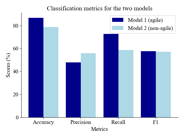
Figure 3: Classification metrics. Estimated unsafe set $\hat{C}$ vs. true failure set $C^{\star}$.

We observe an empirical similarity between the ground truth BRTs and the learned constraints. Additionally, we report quantitative metrics for our classifiers in Fig. 3. These quantitative and qualitative results support our argument that the inferred constraint $\hat{c}_{\text{agile}}(s)$ and $\hat{c}_{\text{non-agile}}(s)$ are indeed approximations of the BRTs for model 1 (agile dynamics) and model 2 (non-agile dynamics) respectively. It is important to note that the classification errors can be attributed to limited expert coverage in certain parts of the state space. This limitation arises from capping the number of start-goal states at $K=150$ (i.e., the total number of tasks) due to the high computational cost of the inner MT-ICL loop, which involves training a full RL model for each task.

5.4.2 ICL Can “Hide” the BRT When the System is Agile

Agile systems are commonly used in the existing ICL literature, leading to the impression that the set inferred from constraint $\hat{c}$ (the set $\hat{C}=\{s\in\mathcal{S}\;|\;1[\hat{c}(s)=\infty\}$) is always equal to the failure set $\mathcal{F}=C^{\star}$. However, we note that this equivalence holds only when $\text{BRT}(\mathcal{F})\approx\mathcal{F}$—i.e., when the system possesses sufficient control authority to consistently steer away from the unsafe set (e.g. model 1 in Fig. 2). For general dynamics (e.g. model 2 in Fig. 2), $\hat{C}\neq\mathcal{F}$ when $\text{BRT}(\mathcal{F})\neq\mathcal{F}$.

5.4.3 The Constraint Inferred via ICL Doesn’t Neccesarily Generalize Across Dynamics

The fact that ICL approximates the BRT leads to another key observation: the inferred constraint may not generalize effectively across different dynamics. For instance, in our setting, we cannot learn a constraint based on model 1 (agile dynamics) and apply it successfully to model 2 (non-agile dynamics), or vice-versa.

Transferring the Learned Constraint from Agile to Non-Agile Systems. Consider a scenario where we have access to expert trajectories of a Dubins car characterized by model 1 (agile). From these demonstrations, we use ICL to derive the constraint $\hat{c}_{\text{agile}}(s)$. We then train an RL policy for a Dubins car with model 2 (non-agile) dynamics on the task of reaching a goal state from a start state using $\hat{c}_{\text{agile}}(s)$ as the constraint. However, as shown in Figs. 2c and 2d, $\hat{c}_{\text{agile}}(s)$ is an under-approximation of $\hat{c}_{\text{non-agile}}(s)$. This under-approximation diminishes the effectiveness of using $\hat{c}_{\text{agile}}(s)$ to generate safe trajectories for our robot during policy exploration, as the robot will likely enter unsafe regions and violate the failure set.

Transferring the Learned Constraint from Non-Agile to Agile Systems. Conversely, using $\hat{c}_{\text{non-agile}}(s)$ as the constraint when training a policy for a robot adhering to model 1 (agile dynamics) can lead to suboptimal control policies with respect to performance metrics such as path length. This is because $\hat{c}_{\text{non-agile}}(s)$ is an overly conservative estimate of the constraint $\hat{c}_{\text{agile}}(s)$ causing the robot to avoid states from which it could actually remain safe leading to overly restrictive policies.

6 Conclusion, Implications, and Future Work

In this work, we have identified that inverse constrained learning (ICL), in fact, approximates the backward reachable tube (BRT) using expert demonstrations, rather than the true failure set. We now argue that this observation has a positive impact from a computational perspective and a negative impact from a transferability perspective.

Implications. First, we note that we can add ICL algorithms to the set of computational tools available to us to calculate BRTs, given a dataset of safe demonstrations, without requiring prior knowledge of the true failure set. Computing a BRT is the first step in many downstream safe control synthesis procedures of popular interest. We also note that having access to a BRT approximator can help speed up policy search, as the set of policies that do not violate the constraint is a subset of the full policy space. Thus, a statistical method should take fewer samples to learn the (safe) optimal policy with this knowledge. However, any BRT (inferred by ICL or otherwise) is dependent on the dynamics of the system and hence cannot be easily used to learn policies on different systems without care. In this sense, learning a BRT rather than the failure set is a double-edged sword.

We also note that the above observations are somewhat surprising from the perspective of inverse reinforcement learning, where one of the key arguments for learning a reward function is transferability across problems (Ng et al., 2000; Swamy et al., 2023; Sapora et al., 2024). However, such transfer arguments often implicitly assume access to a set of higher-level features which are independent of the system’s dynamics on top of which rewards are learned, rather than the raw state space as used in the preceding experiments for learning constraints. Thus, another approach to explore is whether the transferability of constraints would increase if we learn constraints on top of a set of features which are 1) designed to be dynamics-agnostic and 2) for which the target system is able to match the behavior of the expert system, as is common in IRL practice (Ziebart et al., 2008a).

Future Work. Regardless, an interesting direction for future research involves recovering the true constraint (i.e., the failure set $\mathcal{F}$) using constraints that were learned for different systems with varying dynamics. This process is synonymous to removing the dependence of the constraint on the dynamics by integrating over (i.e., marginalizing) the dynamical variables. This could allow disentangling the dynamics and semantics parts of the constraint, allowing better generalization and faster policy search independent of system dynamics. A potential approach to doing so would be to collect expert demonstrations under a variety of dynamics, learn a constraint for each, and then return an aggregate constraint that is the minimum of the learned constraints, implicitly computing an intersection of the BRTs. Such an intersection would approximate the true failure set.

References

- Ames et al. (2019) Aaron D Ames, Samuel Coogan, Magnus Egerstedt, Gennaro Notomista, Koushil Sreenath, and Paulo Tabuada. Control barrier functions: Theory and applications. In 2019 18th European control conference (ECC), pp. 3420–3431. IEEE, 2019.
- Bansal & Tomlin (2021) Somil Bansal and Claire J Tomlin. Deepreach: A deep learning approach to high-dimensional reachability. In 2021 IEEE International Conference on Robotics and Automation (ICRA), pp. 1817–1824. IEEE, 2021.
- Chou et al. (2020) Glen Chou, Dmitry Berenson, and Necmiye Ozay. Learning constraints from demonstrations. In Algorithmic Foundations of Robotics XIII: Proceedings of the 13th Workshop on the Algorithmic Foundations of Robotics 13, pp. 228–245. Springer, 2020.
- Fisac et al. (2015) Jaime F Fisac, Mo Chen, Claire J Tomlin, and S Shankar Sastry. Reach-avoid problems with time-varying dynamics, targets and constraints. In Proceedings of the 18th international conference on hybrid systems: computation and control, pp. 11–20, 2015.
- Hadfield-Menell et al. (2017) Dylan Hadfield-Menell, Smitha Milli, Pieter Abbeel, Stuart J Russell, and Anca Dragan. Inverse reward design. Advances in neural information processing systems, 30, 2017.
- Ho & Ermon (2016) Jonathan Ho and Stefano Ermon. Generative adversarial imitation learning. Advances in neural information processing systems, 29, 2016.
- Howell et al. (2022) Taylor A Howell, Kevin Tracy, Simon Le Cleac’h, and Zachary Manchester. Calipso: A differentiable solver for trajectory optimization with conic and complementarity constraints. In The International Symposium of Robotics Research, pp. 504–521. Springer, 2022.
- Hsu et al. (2023) Kai-Chieh Hsu, Duy Phuong Nguyen, and Jaime Fernandez Fisac. Isaacs: Iterative soft adversarial actor-critic for safety. In Learning for Dynamics and Control Conference, pp. 90–103. PMLR, 2023.
- Huang et al. (2023) Peide Huang, Xilun Zhang, Ziang Cao, Shiqi Liu, Mengdi Xu, Wenhao Ding, Jonathan Francis, Bingqing Chen, and Ding Zhao. What went wrong? closing the sim-to-real gap via differentiable causal discovery. In Conference on Robot Learning, pp. 734–760. PMLR, 2023.
- Hugessen et al. (2024) Adriana Hugessen, Harley Wiltzer, and Glen Berseth. Simplifying constraint inference with inverse reinforcement learning. In The Thirty-eighth Annual Conference on Neural Information Processing Systems, 2024.
- Kim et al. (2023) Konwoo Kim, Gokul Swamy, Zuxin Liu, Ding Zhao, Sanjiban Choudhury, and Steven Z. Wu. Learning shared safety constraints from multi-task demonstrations. In A. Oh, T. Naumann, A. Globerson, K. Saenko, M. Hardt, and S. Levine (eds.), Advances in Neural Information Processing Systems, volume 36, pp. 5808–5826. Curran Associates, Inc., 2023. URL https://proceedings.neurips.cc/paper_files/paper/2023/file/124dde499d62b58e97e42a45b26d7369-Paper-Conference.pdf.
- Lindner et al. (2024) David Lindner, Xin Chen, Sebastian Tschiatschek, Katja Hofmann, and Andreas Krause. Learning safety constraints from demonstrations with unknown rewards. In International Conference on Artificial Intelligence and Statistics, pp. 2386–2394. PMLR, 2024.
- Liu et al. (2024) Guiliang Liu, Sheng Xu, Shicheng Liu, Ashish Gaurav, Sriram Ganapathi Subramanian, and Pascal Poupart. A comprehensive survey on inverse constrained reinforcement learning: Definitions, progress and challenges. arXiv preprint arXiv:2409.07569, 2024.
- Margellos & Lygeros (2011) Kostas Margellos and John Lygeros. Hamilton–jacobi formulation for reach–avoid differential games. IEEE Transactions on automatic control, 56(8):1849–1861, 2011.
- Massey et al. (1990) James Massey et al. Causality, feedback and directed information. In Proc. Int. Symp. Inf. Theory Applic.(ISITA-90), volume 2, 1990.
- McPherson et al. (2021) David L McPherson, Kaylene C Stocking, and S Shankar Sastry. Maximum likelihood constraint inference from stochastic demonstrations. In 2021 IEEE Conference on Control Technology and Applications (CCTA), pp. 1208–1213. IEEE, 2021.
- Mitchell (2004) I. Mitchell. A toolbox of level set methods. http://www. cs. ubc. ca/mitchell/ToolboxLS/toolboxLS. pdf, Tech. Rep. TR-2004-09, 2004.
- Mitchell et al. (2005) Ian M Mitchell, Alexandre M Bayen, and Claire J Tomlin. A time-dependent hamilton-jacobi formulation of reachable sets for continuous dynamic games. IEEE Transactions on automatic control, 50(7):947–957, 2005.
- Ng et al. (2000) Andrew Y Ng, Stuart Russell, et al. Algorithms for inverse reinforcement learning. In Icml, volume 1, pp. 2, 2000.
- Phillips & Dudík (2008) Steven J Phillips and Miroslav Dudík. Modeling of species distributions with maxent: new extensions and a comprehensive evaluation. Ecography, 31(2):161–175, 2008.
- (21) Mohamad Qadri and Michael Kaess. Learning observation models with incremental non-differentiable graph optimizers in the loop for robotics state estimation. In ICML 2023 Workshop on Differentiable Almost Everything: Differentiable Relaxations, Algorithms, Operators, and Simulators.
- Qadri et al. (2022) Mohamad Qadri, Paloma Sodhi, Joshua G Mangelson, Frank Dellaert, and Michael Kaess. Incopt: Incremental constrained optimization using the bayes tree. In 2022 IEEE/RSJ International Conference on Intelligent Robots and Systems (IROS), pp. 6381–6388. IEEE, 2022.
- Qadri et al. (2024) Mohamad Qadri, Zachary Manchester, and Michael Kaess. Learning covariances for estimation with constrained bilevel optimization. In 2024 IEEE International Conference on Robotics and Automation (ICRA), pp. 15951–15957. IEEE, 2024.
- Ren et al. (2024) Juntao Ren, Gokul Swamy, Zhiwei Steven Wu, J Andrew Bagnell, and Sanjiban Choudhury. Hybrid inverse reinforcement learning. arXiv preprint arXiv:2402.08848, 2024.
- Sapora et al. (2024) Silvia Sapora, Gokul Swamy, Chris Lu, Yee Whye Teh, and Jakob Nicolaus Foerster. Evil: Evolution strategies for generalisable imitation learning. arXiv preprint arXiv:2406.11905, 2024.
- Schulman et al. (2017) John Schulman, Filip Wolski, Prafulla Dhariwal, Alec Radford, and Oleg Klimov. Proximal policy optimization algorithms. arXiv preprint arXiv:1707.06347, 2017.
- Scobee & Sastry (2019) Dexter RR Scobee and S Shankar Sastry. Maximum likelihood constraint inference for inverse reinforcement learning. International Conference on Learning Representations, 2019.
- Stanford ASL (2021) Autonomous Systems Lab Stanford ASL. Hj reachability. https://github.com/StanfordASL/hj_reachability, 2021. GitHub repository.
- Stocking et al. (2022) Kaylene C Stocking, D Livingston McPherson, Robert P Matthew, and Claire J Tomlin. Maximum likelihood constraint inference on continuous state spaces. In 2022 International Conference on Robotics and Automation (ICRA), pp. 8598–8604. IEEE, 2022.
- Stooke et al. (2020) Adam Stooke, Joshua Achiam, and Pieter Abbeel. Responsive safety in reinforcement learning by pid lagrangian methods. In International Conference on Machine Learning, pp. 9133–9143. PMLR, 2020.
- Swamy et al. (2021) Gokul Swamy, Sanjiban Choudhury, J Andrew Bagnell, and Steven Wu. Of moments and matching: A game-theoretic framework for closing the imitation gap. In International Conference on Machine Learning, pp. 10022–10032. PMLR, 2021.
- Swamy et al. (2022) Gokul Swamy, Sanjiban Choudhury, J Bagnell, and Steven Z Wu. Sequence model imitation learning with unobserved contexts. Advances in Neural Information Processing Systems, 35:17665–17676, 2022.
- Swamy et al. (2023) Gokul Swamy, David Wu, Sanjiban Choudhury, Drew Bagnell, and Steven Wu. Inverse reinforcement learning without reinforcement learning. In International Conference on Machine Learning, pp. 33299–33318. PMLR, 2023.
- Weng et al. (2022) Jiayi Weng, Huayu Chen, Dong Yan, Kaichao You, Alexis Duburcq, Minghao Zhang, Yi Su, Hang Su, and Jun Zhu. Tianshou: A highly modularized deep reinforcement learning library. Journal of Machine Learning Research, 23(267):1–6, 2022. URL http://jmlr.org/papers/v23/21-1127.html.
- Wu et al. (2024) Runzhe Wu, Yiding Chen, Gokul Swamy, Kianté Brantley, and Wen Sun. Diffusing states and matching scores: A new framework for imitation learning. arXiv preprint arXiv:2410.13855, 2024.
- Xiao & Belta (2021) Wei Xiao and Calin Belta. High-order control barrier functions. IEEE Transactions on Automatic Control, 67(7):3655–3662, 2021.
- Ziebart (2010) Brian D Ziebart. Modeling purposeful adaptive behavior with the principle of maximum causal entropy. Carnegie Mellon University, 2010.
- Ziebart et al. (2008a) Brian D Ziebart, Andrew L Maas, J Andrew Bagnell, Anind K Dey, et al. Maximum entropy inverse reinforcement learning. In Aaai, volume 8, pp. 1433–1438. Chicago, IL, USA, 2008a.
- Ziebart et al. (2008b) Brian D Ziebart, Andrew L Maas, Anind K Dey, and J Andrew Bagnell. Navigate like a cabbie: Probabilistic reasoning from observed context-aware behavior. In Proceedings of the 10th international conference on Ubiquitous computing, pp. 322–331, 2008b.