Towards Sharper Information-theoretic Generalization Bounds for Meta-Learning

Abstract

In recent years, information-theoretic generalization bounds have emerged as a promising approach for analyzing the generalization capabilities of meta-learning algorithms. However, existing results are confined to two-step bounds, failing to provide a sharper characterization of the meta-generalization gap that simultaneously accounts for environment-level and task-level dependencies. This paper addresses this fundamental limitation by establishing novel single-step information-theoretic bounds for meta-learning. Our bounds exhibit substantial advantages over prior MI- and CMI-based bounds, especially in terms of tightness, scaling behavior associated with sampled tasks and samples per task, and computational tractability. Furthermore, we provide novel theoretical insights into the generalization behavior of two classes of noise and iterative meta-learning algorithms via gradient covariance analysis, where the meta-learner uses either the entire meta-training data (e.g., Reptile), or separate training and test data within the task (e.g., model agnostic meta-learning (MAML)). Numerical results validate the effectiveness of the derived bounds in capturing the generalization dynamics of meta-learning.

1 Introduction

Meta-learning, also known as learning to learn, has emerged as a prevalent paradigm for rapidly adapting to new tasks, by leveraging prior knowledge extracted from multiple inherently relevant tasks Hospedales et al. (2021); Hu et al. (2023); Lake & Baroni (2023). Concretely, the meta-learner has access to training data from tasks observed within a common task environment to learn meta-hyperparameters, which can then fine-tune task-specific parameters for improving performance on a novel task. Extensive efforts have recently been dedicated to optimizing their empirical behavior on the meta-training data, with the goal of achieving minimal meta-training error Zhang et al. (2022); Abbas et al. (2022); Wang et al. (2023). However, lower meta-training errors do not necessarily ensure excellent performance on previously unseen tasks. Therefore, it is crucial to establish upper bounds on the meta-generalization gap—the difference between the population and empirical risks of the meta-hypothesis—to guarantee the generalization of meta-learning.

Information-theoretic generalization bounds Xu & Raginsky (2017); Steinke & Zakynthinou (2020); Hellström & Durisi (2022b); Wang & Mao (2023), expressed by distribution- and algorithm-dependent information measures, have attracted widespread attention for their capability of precisely characterizing the generalization properties of learning algorithms. Along the lines of work Xu & Raginsky (2017); Bu et al. (2020), Jose & Simeone (2021) initially establish the two-step generalization bounds for meta-learning by separately bounding the task-environment and per-task generalization errors within the framework of conventional learning. Such a two-step bound typically overlooks the dependencies between the meta-hypothesis and task-specific hypotheses, resulting in unfavorable scaling w.r.t the number of sampled tasks and in-task samples. Substantial advancements have been made by Chen et al. (2021); Bu et al. (2023), who immediately bound the meta-generalization gap through the mutual information (MI) between both task-specific and meta hypotheses and the meta-training data, yielding tighter upper bounds than that of Jose & Simeone (2021). Building on the conditional mutual information (CMI) framework Steinke & Zakynthinou (2020) and the same two-step analysis of Jose & Simeone (2021), subsequent work further tightens previous meta-generalization bounds by quantifying the information contained in the partial parameters Rezazadeh et al. (2021) or the evaluated losses Hellström & Durisi (2022a) about the selected meta-training data, given the full meta-supersample set. Despite remarkable success, it is noteworthy that the aforementioned work can subsequently be strengthened and refined through the lens of single-step bounds.

This paper provides a unified information-theoretic generalization analysis for meta-learning, along with a comparison to existing results presented in Table 1. The main contributions are summarized as follows:

Table 1: Existing information-theoretic generalization bounds for meta-learning ($\ast$-binary KL divergence bound; $\star$-fast-rate bound).

Information Measure	Related Work	Meta Generalization Bound	Analysis Tool
Input-output MI	Jose & Simeone (2021)	$\mathcal{O}(\sqrt{I(U;T_{\mathbb{M}}^{\mathbb{N}})/n}+\sqrt{I(W;T_{\mathbb{M}}|\tau)/m})$	Two-step derivation
	Chen et al. (2021)	$\mathcal{O}(\sqrt{I(U,W_{\mathbb{N}};T_{\mathbb{M}}^{\mathbb{N}})/nm})$	Single-step derivation
	Bu et al. (2023)
Samplewise MI	Ours (Thm. 3.2)	$\mathcal{O}\big{(}\frac{1}{nm}\sum_{i,j=1}^{n,m}\sqrt{I(U,W_{i};Z^{i}_{j})}\big{)}$	Single-step derivation Random subset
1-4
CMI	Rezazadeh et al. (2021)	$\mathcal{O}\Big{(}\sqrt{I(U;S_{\mathbb{N}},S_{\mathbb{M}}^{\mathbb{N}}|T_{2\mathbb{M}}^{2\mathbb{N}})/n}+\frac{1}{n}\sum_{i=1}^{n}\sqrt{I(W_{i};S^{i}_{\mathbb{M}}|T_{2\mathbb{M}}^{2\mathbb{N}},S_{i})/m}\Big{)}$	Two-step derivation ($n+nm$) Sample marks
	Ours (Thm. 3.5)	$\mathcal{O}(\sqrt{I(U,W_{\mathbb{N}};\tilde{S}_{\mathbb{N}},S_{\mathbb{M}}|T_{2\mathbb{M}}^{2\mathbb{N}})/nm})$	Single-step derivation Random subset ($\bm{n+m}$) Sample marks
	Ours (Thm. 3.7)	$\ast\mathcal{O}(\frac{1}{nm}\sum_{i,j=1}^{n,m}I(U,W_{i};\tilde{S}_{i},S_{j}|T_{2\mathbb{M}}^{2\mathbb{N}}))$
	Ours (Thm. 3.8)	$\star\mathcal{O}(\frac{1}{nm}\sum_{i,j=1}^{n,m}I(U,W_{i};\tilde{S}_{i},S_{j}|T_{2\mathbb{M}}^{2\mathbb{N}}))$
1-4
e-CMI	Hellström & Durisi (2022a)	$\mathcal{O}\Big{(}\frac{1}{nm}\sum_{i,j=1}^{n,m}\big{(}\sqrt{I(\tilde{L}^{i}_{j,S^{i}_{j}};\tilde{S}_{i}|T_{2\mathbb{M}}^{2\mathbb{N}},S^{i}_{j})}+\sqrt{I(\tilde{L}^{i,\bar{\tilde{S}}_{i}}_{j};\bar{S}^{i}_{j}|T_{2\mathbb{M}}^{2\mathbb{N}},\tilde{S}_{i})}\big{)}\Big{)}$	Two-step derivation ($n+nm$) Sample marks
	Ours (Thm. 3.10)	$\mathcal{O}\Big{(}\frac{1}{nm}\sum_{i,j=1}^{n,m}\sqrt{I(L^{i}_{j};\tilde{S}_{i},S_{j}|T_{2\mathbb{M}}^{2\mathbb{N}})}\Big{)}$	Single-step derivation ($\bm{n+m}$) Sample marks
	Ours (Thm. 3.12)	$\ast\mathcal{O}\Big{(}\frac{1}{nm}\sum_{i,j=1}^{n,m}I(L^{i}_{j};\tilde{S}_{i},S_{j})\Big{)}$
1-4
Loss-difference CMI	Ours (Thm. 3.13)	$\mathcal{O}\Big{(}\frac{1}{nm}\sum_{i,j=1}^{n,m}\sqrt{I(\Delta_{i,j}^{\Psi};S_{j}|T_{2\mathbb{M}}^{2\mathbb{N}})}\Big{)}$	Single-step derivation ($\bm{n+m}$) Sample marks
Loss-difference MI	Ours (Thm. 3.14)	$\mathcal{O}\Big{(}\frac{1}{nm}\sum_{i,j=1}^{n,m}\sqrt{I(\Delta_{i,j}^{\Psi};S_{j})}\Big{)}$
Single-Loss MI	Ours (Thm. 3.16)	$\star\mathcal{O}(\frac{1}{nm}\sum_{i,j=1}^{n,m}\min\{I(L_{i,j}^{\Psi};S_{j}),2I(L_{i,j}^{\Psi_{+}};S_{j})\})$
	Ours (Thm. 3.18)	$\star\mathcal{O}(C_{1}V(\gamma)+\frac{1}{nm}\sum_{i,j=1}^{n,m}\min\{I(L_{i,j}^{\Psi};S_{j}),2I(L_{i,j}^{\Psi_{+}};S_{j})\})$

• We establish novel single-step information-theoretic generalization bounds for meta-learning by leveraging random subsets and the supersample method. Our bounds, expressed in terms of information measures that simultaneously integrate meta-parameters, task-specific parameters, and sample subsets, tighten existing bounds and yield a more favorable scaling rate of $\mathcal{O}(1/\sqrt{nm})$, where $n$ and $m$ represent the number of tasks and the number of samples per task, respectively.

• We develop loss difference-based meta-generalization bounds through both unconditional and conditional information measures. The derived bounds exclusively involve two one-dimensional variables, making them computationally feasible and more rigorous than previous MI- and CMI-based bounds of meta-learning. Furthermore, we introduce a novel fast-rate bound by employing the weighted generalization error, achieving a faster convergence rate of $\mathcal{O}(1/nm)$ in the interpolating regime. This fast-rate result is further generalized to non-interpolating settings through the development of variance-based bounds.

• Our theoretical framework generally applies to a broad range of meta-learning paradigms, including those using the entire meta-training data as well as those employing within-task train-test partitions. In particular, we derive tighter algorithm-dependent bounds for both learning paradigms via the conditional gradient variance, exhibiting substantial superiority over bounds that rely on the gradient norm and gradient variance. Our results provide novel theoretical insight into the learning trajectory of noisy and iterative algorithms within the context of meta-learning.

• Empirical studies on synthetic and real-world datasets validate the closeness between the generalization error and the derived bounds.

2 Preliminaries

Basic Notations.

We denote random variables by capital letters (e.g., $X$), their sepcific values by lowercase letters (e.g., $x$), and the corresponding domains by calligraphic letters (e.g., $\mathcal{X}$). Let $P_{X,Y}$ denote the joint distribution of variable $(X,Y)$, $P_{X}$ denote the marginal probability distribution of $X$, and $P_{X|Y}$ be the conditional distribution of $X$ given $Y$, where $P_{X|y}$ denotes the one conditioning on a sepcific value $Y=y$. Similarly, denote by $\mathbb{E}_{X}$, $\mathrm{Var}_{X}$, and $\mathrm{Cov}_{X}$ the expectation, variance, and covariance matrix taken over $X\sim P_{X}$. Given probability measures $P$ and $Q$, we define the Kullback-Leibler (KL) divergence of $P$ w.r.t $Q$ as $D(P\|Q)=\int\log\frac{dP}{dQ}dP$. For two Bernoulli distributions with parameters $p$ and $q$, we refer to $d(p\|q)=p\log(\frac{p}{q})+(1-p)\log(\frac{1-p}{1-q})$ as the binary KL divergence. Let $I(X;Y)$ be the MI between variables $X$ and $Y$, and $I(X;Y|Z)=\mathbb{E}_{z}[I^{z}(X;Y)]$ be the CMI conditioned on $Z$, where $I^{z}(X;Y)=D(P_{X,Y|z}\|P_{X|z}P_{Y_{z}})$ denotes the disintegrated MI. Let $\log$ be the logarithmic function with base $e$ and $\mathbf{1}_{d}$ denote a $d$-dimensional vector of ones.

Meta Learning.

The goal of meta-learning is to automatically infer an output hypothesis $U\in\mathcal{U}$ from data across multiple related tasks, enabling rapid and efficient adaptation to novel, previously unseen tasks Chen et al. (2021); Rezazadeh et al. (2021); Hellström & Durisi (2022a), where $\mathcal{U}$ represents the parametrized hypothesis space. Consider a common task environment $\mathcal{T}$ defined by a probability distribution $P_{\mathcal{T}}$. Assume that we have $n$ different observation tasks, denoted as $\tau_{\mathbb{N}}=(\tau_{1},\ldots,\tau_{n})$, independently drawn from the distribution $P_{\mathcal{T}}$. For each task $\tau_{i}$, $i\in[n]$, further draw $m$ i.i.d. training samples from a data-generation distribution $P_{Z|\tau_{i}}$ over the sample space $\mathcal{Z}$ related to task $\tau_{i}$, denoted as $T_{\mathbb{M}}^{i}=\{Z^{i}_{j}\}^{m}_{j=1}$. The complete meta-training dataset consisting of $n$ tasks with $m$ in-task samples is then expressed by $T_{\mathbb{M}}^{\mathbb{N}}=\{T_{\mathbb{M}}^{i}\}^{n}_{i=1}$. A widely adopted approach for learning an optimal meta-hypothesis $U$ is to minimize the following empirical meta-risk:

$$\mathcal{R}(U,T_{\mathbb{M}}^{\mathbb{N}})=\frac{1}{n}\sum_{i=1}^{n}\mathbb{E}_{W_{i}\sim P_{W_{i}|U,T_{\mathbb{M}}^{i}}}\big{[}\mathcal{R}(U,W_{i},T_{\mathbb{M}}^{i})\big{]},$$

where $W_{i}\in\mathcal{W}$ denotes the task-specific parameter tuned via $U$ and $T_{\mathbb{M}}^{i}$, in which $\mathcal{W}$ denotes its parameter space, and $\mathcal{R}(U,W_{i},T_{\mathbb{M}}^{i})$ is the task-specific empirical risk, defined by

$$\mathcal{R}(U,W_{i},T_{\mathbb{M}}^{i})=\frac{1}{m}\sum_{j=1}^{m}\ell(U,W_{i},Z^{i}_{j}),$$

where $\ell:\mathcal{U}\times\mathcal{W}\times\mathcal{Z}\rightarrow\mathbb{R}^{+}$ is a given loss function.

The generalization performance of $U$ on new tasks is then measured by the population meta-risk :

$$\mathcal{R}(U,\mathcal{T})=\mathbb{E}_{\tau\sim P_{\mathcal{T}}}\mathbb{E}_{T_{\mathbb{M}}\sim P_{Z|\tau}}\big{[}\mathbb{E}_{P_{W|T_{\mathbb{M}},U}}[\mathcal{R}(U,W,P_{Z|\tau})]\big{]},$$

where $\mathcal{R}(U,W,P_{Z|\tau})=\mathbb{E}_{Z\sim P_{Z|\tau}}[\ell(U,W,Z)]$ represents the population risk of a novel task $\tau$ over unseen samples $Z\sim P_{Z|\tau}$.

We define the meta-generalization gap by

$$\overline{\mathrm{gen}}=\mathbb{E}_{U,T_{\mathbb{M}}^{\mathbb{N}}}[\mathcal{R}(U,\mathcal{T})-\mathcal{R}(U,T_{\mathbb{M}}^{\mathbb{N}})],$$

which quantifies the discrepancy between the empirical and population meta-risks. The less meta-generalization gap indicates that on average or with high probability, the empirical performance of the meta hypothesis $U$ on the training data could serve as a reliable measure of its generalization ability. Bounding the meta-generalization gap is thus the focus of this paper, to provide generalization guarantees for meta-learning. To simplify the notation, let $\mathcal{R}_{\mathcal{T}}:=\mathbb{E}_{U,T_{\mathbb{M}}^{\mathbb{N}}}\big{[}\mathcal{R}(U,\mathcal{T})]$ and $\hat{\mathcal{R}}:=\mathbb{E}_{U,T_{\mathbb{M}}^{\mathbb{N}}}\big{[}\mathcal{R}(U,T_{\mathbb{M}}^{\mathbb{N}})]$.

CMI-Based Framework.

The CMI framework is originally investigated in Steinke & Zakynthinou (2020) for generalization analysis. Let $T^{2\mathbb{N}}_{2\mathbb{M}}=\{T^{i,0}_{2\mathbb{M}},T^{i,1}_{2\mathbb{M}}\}_{i=1}^{n}$ be the meta-supersample dataset across $2\times n$ different tasks, where $T^{i,0}_{2\mathbb{M}}=\{(\tilde{Z}^{i,0}_{j,0},\tilde{Z}^{i,0}_{j,1})\}_{j=1}^{m},T^{i,1}_{2\mathbb{M}}=\{(\tilde{Z}^{i,1}_{j,0},\tilde{Z}^{i,1}_{j,1})\}_{j=1}^{m}\in\mathcal{Z}^{m\times 2}$ denote the per-task supersample set consisting of $2\times m$ i.i.d. samples drawn from $P_{Z|\tau_{i}}$. Further let $\tilde{S}_{\mathbb{N}}=\{\tilde{S}_{i}\}_{i=1}^{n}\sim\mathrm{Unif}(\{0,1\}^{n})$ and $S_{\mathbb{M}}=\{S_{j}\}_{j=1}^{m}\sim\mathrm{Unif}(\{0,1\}^{m})$ be the membership vectors independent of $T^{2\mathbb{N}}_{2\mathbb{M}}$, and $\bar{\tilde{S}}_{\mathbb{N}}=\{1-\tilde{S}_{i}\}_{i=1}^{n}$ and $\bar{S}_{\mathbb{M}}=\{1-S_{j}\}_{j=1}^{m}$ be the modulo-2 complement of $\tilde{S}_{\mathbb{N}}$ and $S_{\mathbb{M}}$, respectively. We utilize the variables $(\tilde{S}_{\mathbb{N}},S_{\mathbb{M}})$ and $(\bar{\tilde{S}}_{\mathbb{N}},\bar{S}_{\mathbb{M}})$ to separate $T^{2\mathbb{N}}_{2\mathbb{M}}$ into the meta-training dataset $T^{2\mathbb{N},\tilde{S}_{\mathbb{N}}}_{2\mathbb{M},S_{\mathbb{M}}}=\{\tilde{Z}^{i,\tilde{S}_{i}}_{j,S_{j}}\}_{i,j=1}^{n,m}$ and the meta-test dataset $T^{2\mathbb{N},\bar{\tilde{S}}_{\mathbb{N}}}_{2\mathbb{M},\bar{S}_{\mathbb{M}}}=\{\tilde{Z}^{i,\bar{\tilde{S}}_{i}}_{j,\bar{S}_{j}}\}_{i,j=1}^{n,m}$. Analogously, denote by $T^{2\mathbb{N},\bar{\tilde{S}}_{\mathbb{N}}}_{2\mathbb{M},S_{\mathbb{M}}}$ the training dataset for the meta-test task and $T^{2\mathbb{N},\tilde{S}_{\mathbb{N}}}_{2\mathbb{M},\bar{S}_{\mathbb{M}}}$ the test dataset for the meta-training tasks.

Let $L^{i,\tilde{S}_{i}}_{j,S_{j}}\triangleq\ell(U,W_{i},\tilde{Z}^{i,\tilde{S}_{i}}_{j,S_{j}})$ and $L^{i,\bar{\tilde{S}}_{i}}_{j,\bar{S}_{j}}\triangleq\ell(U,W_{i},\tilde{Z}^{i,\bar{\tilde{S}}_{i}}_{j,\bar{S}_{j}})$ represent the samplewise losses on the meta-training and meta-test data, respectively. Further let $\Psi=\{\Psi_{i,j}=\tilde{S}_{i}\oplus S_{j}\}_{i,j=1}^{n,m}$ and $\tilde{\Psi}=\{\tilde{\Psi}_{i,j}=1\oplus\Psi_{i,j}\}_{i,j=1}^{n,m}$, where $\oplus$ is the XOR operation. To simplify the notations, we denote $L_{j,1}^{i,\tilde{\Psi}_{i,j}}$ and $L_{j,0}^{i,\tilde{\Psi}_{i,j}}$ as $L_{i,j}^{\Psi_{+}}$ and $L_{i,j}^{\Psi_{-}}$. $L^{\Psi}_{i,j}=\{L_{i,j}^{\Psi_{+}},L_{i,j}^{\Psi_{-}}\}$ then represents a pair of losses, and $\Delta^{\Psi}_{i,j}=L_{i,j}^{\Psi_{+}}-L_{i,j}^{\Psi_{-}}$ is their difference. We define the loss pairs on the full meta-supersample set as $L_{2\mathbb{M}}^{2\mathbb{N}}=\{L^{i}_{j}=(L^{i,0}_{j,0},L^{i,1}_{j,1},L^{i,1}_{j,0},L^{i,0}_{j,1})\}_{i,j=1}^{n,m}$.

3 Information-theoretic Generalization Bounds for Meta-learning

3.1 Generalization Bounds with Input-output MI

The pioneering work of Chen et al. (2021) provides a rigorous theoretical characterization of meta-generalization by developing the MI-based generalization bound incorporating both environment-level and task-level dependencies:

Lemma 3.1.

[Theorem 5.1 in Chen et al. (2021)] Assume that $\ell(U,W,Z)$ is $\sigma$-sub-gaussian for all $Z\sim P_{Z|\tau},\tau\sim P_{\mathcal{T}}$, $U\in\mathcal{U},W\in\mathcal{W}$, then

$$|\overline{\mathrm{gen}}|\leq\sqrt{\frac{2\sigma^{2}}{nm}I(U,W_{\mathbb{N}};T^{\mathbb{N}}_{\mathbb{M}})},$$ (1)

where $W_{\mathbb{N}}=(W_{1},\ldots,W_{n})$ denotes task-specific parameters across $n$ tasks.

Lemma 3.1 connects the meta-generalization gap to the MI between the environment- and task-level output hypotheses $(U,W_{\mathbb{N}})$ and the meta-training data $T^{\mathbb{N}}_{\mathbb{M}}$, achieving improvements over the foundational work of Jose & Simeone (2021) in terms of the scaling rate $\mathcal{O}(1/\sqrt{nm})$. However, such an upper bound coincides with the “on-average” stability Shalev-Shwartz et al. (2010), potentially leading to meaningless results when the output hypothesis is deterministic, namely, $I(U,W_{\mathbb{N}};T^{\mathbb{N}}_{\mathbb{M}})=\infty$ for unique minimizer $(U,W_{\mathbb{N}})$ of the empirical meta-risk.

Building upon the random subset methodology Harutyunyan et al. (2021), we measure the information contained in randomly selected subsets of both tasks and in-task samples instead of the entire training dataset as in Chen et al. (2021), thereby achieving “point-wise” stability Raginsky et al. (2016); Bu et al. (2020) and yielding the following improved bound:

Theorem 3.2.

Let $\mathbb{K}$ and $\mathbb{J}$ be random subsets of $[n]$ and $[m]$ with sizes $\zeta$ and $\xi$, respectively, independent of $T^{\mathbb{N}}_{\mathbb{M}}$ and $(U,W_{\mathbb{N}})$. Assume that $\ell(U,W,Z)$ is $\sigma$-sub-gaussian for all $Z\sim P_{Z|\tau},\tau\sim P_{\mathcal{T}}$, $U\in\mathcal{U},W\in\mathcal{W}$, then

$$|\overline{\mathrm{gen}}|\leq\mathbb{E}_{K\sim\mathbb{K},J\sim\mathbb{J}}\sqrt{\frac{2\sigma^{2}}{\zeta\xi}I(U,W_{K};T^{K}_{J})}.$$

Theorem 3.2 coincides with the inferences derived by Xu & Raginsky (2017); Harutyunyan et al. (2021): the less the output hypotheses depends on the input data, the better the learning algorithm generalizes. In particular, substituting $\zeta=\xi=1$ yields the samplewise MI bound:

$$|\overline{\mathrm{gen}}|\leq\frac{1}{nm}\sum_{i,j=1}^{n,m}\sqrt{2\sigma^{2}I(U,W_{i};Z^{i}_{j})},$$

thereby enhancing the bound in Chen et al. (2021); Bu et al. (2023) by replacing $I(U,W_{\mathbb{N}};T^{\mathbb{N}}_{\mathbb{M}})$ with $I(U,W_{i};Z^{i}_{j})$. Taking $\zeta=n$ and $\xi=m$, the derived bound recovers the generalization bound of Lemma 3.1, and can be upper-bounded by

$$|\overline{\mathrm{gen}}|\leq\sqrt{\frac{2\sigma^{2}}{mn}I(U;T^{\mathbb{N}}_{\mathbb{M}})}+\sqrt{\frac{2\sigma^{2}}{mn}\sum_{i=1}^{n}I(W_{i};T^{i}_{\mathbb{M}}|U)}.$$

Notably, for the asymptotic regime where $n\rightarrow\infty$ while $m$ remains finite, this upper bound will reduce to the single task scenario: $\sqrt{\frac{2\sigma^{2}}{mn}\sum_{i=1}^{n}I(W_{i};T^{i}_{\mathbb{M}}|U)}$, being more rigorous than that of standard single-task learning Xu & Raginsky (2017); Russo & Zou (2019). Let $I(W;T^{\mathbb{N}}_{\mathbb{M}})$ denote the mutual information of single-task learning. It is evident that $I(W;T^{\mathbb{N}}_{\mathbb{M}})\geq I(W;T^{\mathbb{N}}_{\mathbb{M}}|U)\approx\frac{1}{n}\sum_{i=1}^{n}I(W_{i};T^{i}_{\mathbb{M}}|U)$, thus showcasing the statistical advantage of meta-learning.

It is worth noting that the optimal choice of $\zeta$ and $\xi$ values for rigid bounds is not immediately obvious, as smaller values reduce both the denominator and the MI term. The following proposition has shown that the upper bound in Theorem 3.2 is non-decreasing w.r.t $\zeta$ and $\xi$, implying that the smallest $\zeta$ and $\xi$, namely $\zeta=\xi=1$, yields the tightest bound.

Proposition 3.3.

Let $\zeta\in[n-1]$, $\xi\in[m-1]$, and $\mathbb{K}$ and $\mathbb{J}$ be random subsets of $[n]$ and $[m]$ with sizes $\zeta$ and $\xi$, respectively. Further, let $\mathbb{K}^{\prime}$ and $\mathbb{J}^{\prime}$ be random subsets with sizes $\zeta+1$ and $\xi+1$, respectively. If $g:\mathbb{R}\rightarrow\mathbb{R}$ is any non-decreasing concave function, then

$$\mathbb{E}_{K\sim\mathbb{K},J\sim\mathbb{J}}g\left(\frac{1}{\zeta\xi}I(U,W_{K};T^{K}_{J})\right)\leq\mathbb{E}_{K^{\prime}\sim\mathbb{K}^{\prime},J^{\prime}\sim\mathbb{J}^{\prime}}g\left(\frac{1}{(\zeta+1)(\xi+1)}I(U,W_{K^{\prime}};T^{K^{\prime}}_{J^{\prime}})\right).$$

Applying $g(x)=\sqrt{x}$ does indeed jusify that $\zeta=1$ and $\xi=1$ are the optimal values for minimizing the generalization bound in Theorem 3.2.

3.2 Generalization Bounds with CMI

A remarkable advance made by Rezazadeh et al. (2021) extends the conditional mutual information (CMI) methodology initially introduced in Steinke & Zakynthinou (2020) to meta-learning scenario, obtaining a sharper bound:

Lemma 3.4 (Theorem 1 in Rezazadeh et al. (2021)).

Assume that the loss function takes values in $[0,1]$, then

$$|\overline{\mathrm{gen}}|\leq\sqrt{\frac{2}{n}I(U;\tilde{S}_{\mathbb{N}},S^{\mathbb{N}}_{\mathbb{M}}|T^{2\mathbb{N}}_{2\mathbb{M}})}+\frac{1}{n}\sum_{i=1}^{n}\sqrt{\frac{2}{m}I(W_{i};S_{\mathbb{M}}^{i}|T^{2\mathbb{N}}_{2\mathbb{M}},\tilde{S}_{i})},$$ (2)

where $S^{\mathbb{N}}_{\mathbb{M}}=\{S_{\mathbb{M}}^{i}\}_{i=1}^{n},S_{\mathbb{M}}^{i}=\{S_{j}^{i}\}_{j=1}^{m}$ is the binary variable.

Lemma 3.4 leverages the “two-step” derivation, separately bounding the environment-level and task-level generalization gaps through two CMI terms $I(U;S_{\mathbb{N}},S^{\mathbb{N}}_{\mathbb{M}}|T^{2\mathbb{N}}_{2\mathbb{M}})$ and $I(W;S_{\mathbb{M}}^{i}|T^{2\mathbb{N}}_{2\mathbb{M}},S_{i})$. While the improvement is achieved by introducing binary variables, the neglect of the dependencies between the meta-hypothesis $U$ and the task-specific hypotheses $W_{1},\ldots,W_{n}$ leads to an undesirable scaling rate w.r.t the task size $n$ and the sample size $m$ per task. Additionally, the CMI bound in Lemma 3.4 involves $n+nm$ binary random variables ($\tilde{S}_{\mathbb{N}}$ and $S^{\mathbb{N}}_{\mathbb{M}}$), potentially exhibiting high computational complexity as $n$ and $m$ increases.

We propose a unified analysis to immediately bound the meta-generalization gap within the CMI framework Steinke & Zakynthinou (2020) by incorporating random subset techniques Harutyunyan et al. (2021). Our method requires only $n+m$ binary variables and provides tighter bounds than conventional two-step analyses.

Theorem 3.5.

Let $\mathbb{K}$ and $\mathbb{J}$ be random subsets of $[n]$ and $[m]$ with sizes $\zeta$ and $\xi$, respectively. If the loss function $\ell(\cdot,\cdot,\cdot)$ is bounded within $[0,1]$, then

$$|\overline{\mathrm{gen}}|\leq\mathbb{E}_{T_{2\mathbb{M}}^{2\mathbb{N}},K\sim\mathbb{K},J\sim\mathbb{J}}\sqrt{\frac{2}{\zeta\xi}I^{T_{2\mathbb{M}}^{2\mathbb{N}}}(U,W_{K};\tilde{S}_{K},S_{J})},$$

where $W_{K}=\{W_{i}\}_{i\in K}$, $\tilde{S}_{K}=\{\tilde{S}_{i}\}_{i\in K}$, and $S_{J}=\{S_{j}\}_{j\in J}$.

Notice that when $\zeta=n$ and $\xi=m$, Theorem 3.5 bounds the meta-generalization gap through the CMI between the hypotheses $(U,W_{\mathbb{N}})$ and binary variables $\tilde{S}_{\mathbb{N}},S_{\mathbb{M}}$, conditioning on the meta-supersample $T_{2\mathbb{M}}^{2\mathbb{N}}$. This result not only tightens the MI-based bound, but also achieves a more favorable scaling rate than the existing CMI-based bound. On the one hand, it can be shown that the CMI term $I(U,W_{\mathbb{N}};\tilde{S}_{\mathbb{N}},S_{\mathbb{M}}|T_{2\mathbb{M}}^{2\mathbb{N}})$ consistently provides a tighter upper bound than the MI term $I(U,W_{\mathbb{N}};T_{2\mathbb{M},S_{\mathbb{M}}}^{2\mathbb{N},\tilde{S}_{\mathbb{N}}})$ in Chen et al. (2021); Bu et al. (2023): by the Markov chain $(T_{2\mathbb{M}}^{2\mathbb{N}},\tilde{S}_{\mathbb{N}},S_{\mathbb{M}})-T_{2\mathbb{M},S_{\mathbb{M}}}^{2\mathbb{N},\tilde{S}_{\mathbb{N}}}-(U,W_{\mathbb{N}})$, it is obvious that $I(U,W_{\mathbb{N}};T_{2\mathbb{M},S_{\mathbb{M}}}^{2\mathbb{N},\tilde{S}_{\mathbb{N}}})=I(U,W_{\mathbb{N}};T_{2\mathbb{M}}^{2\mathbb{N}},\tilde{S}_{\mathbb{N}},S_{\mathbb{M}})=I(U,W_{\mathbb{N}};\tilde{S}_{\mathbb{N}},S_{\mathbb{M}}|T_{2\mathbb{M}}^{2\mathbb{N}})+I(U,W_{\mathbb{N}};T_{2\mathbb{M}}^{2\mathbb{N}})\geq I(U,W_{\mathbb{N}};\tilde{S}_{\mathbb{N}},S_{\mathbb{M}}|T_{2\mathbb{M}}^{2\mathbb{N}})$. On the other hand, the upper bound in Theorem 3.5 exhibit a desirable convergence rate of $\mathcal{O}(\frac{1}{\sqrt{nm}})$ instead of $\mathcal{O}(\max\{\frac{1}{\sqrt{n}},\frac{1}{\sqrt{m}}\})$ in Rezazadeh et al. (2021). Furthermore, the less dependence on $\tilde{S}_{\mathbb{N}}$ and $S_{\mathbb{M}}$ facilitates a computationally tractable bound. For the case of $\zeta=\xi=1$, one could obtain the samplewise CMI bound for meta-learning:

$$|\overline{\mathrm{gen}}|\leq\mathbb{E}_{T_{2\mathbb{M}}^{2\mathbb{N}}}\frac{1}{nm}\sum_{i,j=1}^{n,m}\sqrt{2I^{T_{2\mathbb{M}}^{2\mathbb{N}}}(U,W_{i};\tilde{S}_{i},S_{j})},$$

which is further upper-bounded by

$$\frac{1}{nm}\sum_{i,j=1}^{n,m}\Big{(}\sqrt{2I(U;\tilde{S}_{i},S_{j}|T_{2\mathbb{M}}^{2\mathbb{N}})}+\sqrt{2I(W_{i};\tilde{S}_{i},S_{j}|T_{2\mathbb{M}}^{2\mathbb{N}},U)}\Big{)},$$ (3)

applying the chain rule and Jensen’s inequality. As the task size $n$ approaches infinity and the sample size $m$ per task is finite, the first term in (3) reduces to zero, while the second term remains non-zero and can be smaller than the CMI of single-task learning Steinke & Zakynthinou (2020); Harutyunyan et al. (2021). Similarly, let $I(W;\tilde{S},S|T_{2\mathbb{M}}^{2\mathbb{N}})$ denote the CMI of single-task learning, we prove that $I(W;\tilde{S},S|T_{2\mathbb{M}}^{2\mathbb{N}})\geq I(W;\tilde{S},S|T_{2\mathbb{M}}^{2\mathbb{N}},U)\approx\frac{1}{nm}\sum_{i,j=1}^{m}I(W_{i};\tilde{S}_{i},S_{j}|T_{2\mathbb{M}}^{2\mathbb{N}},U)$. For a constant number $n$ and an infinite $m$, the upper bound (3) would converge to zero. Therefore, our theoretical results also demonstrate the advantages of meta-learning over single-task learning.

Extending the analysis of Proposition 3.3 to the disintegrated MI $I^{T_{2\mathbb{M}}^{2\mathbb{N}}}(U,W_{K};\tilde{S}_{K},S_{J})$, we obtain the following monotonic property related to Theorem 3.5:

Proposition 3.6.

Let $\zeta\in[n-1]$, $\xi\in[m-1]$, and $\mathbb{K}$ and $\mathbb{J}$ be random subsets of $[n]$ and $[m]$ with sizes $\zeta$ and $\xi$, respectively. Further, let $\mathbb{K}^{\prime}$ and $\mathbb{J}^{\prime}$ be random subsets with sizes $\zeta+1$ and $\xi+1$, respectively. If $g:\mathbb{R}\rightarrow\mathbb{R}$ is any non-decreasing concave function, then for $T_{2\mathbb{M}}^{2\mathbb{N}}\sim\{P_{Z|\tau_{i}}\}_{i=1}^{n}$ over $\mathcal{Z}^{2n\times 2m}$,

$$\mathbb{E}_{K\sim\mathbb{K},J\sim\mathbb{J}}g\left(\frac{1}{\zeta\xi}I^{T_{2\mathbb{M}}^{2\mathbb{N}}}(U,W_{K};\tilde{S}_{K},S_{J})\right)\leq\mathbb{E}_{K^{\prime}\sim\mathbb{K}^{\prime},J^{\prime}\sim\mathbb{J}^{\prime}}g\left(\frac{1}{(\zeta+1)(\xi+1)}I^{T_{2\mathbb{M}}^{2\mathbb{N}}}(U,W_{K^{\prime}};\tilde{S}_{K^{\prime}},S_{J^{\prime}})\right).$$

By leveraging Proposition 3.6 with $g(x)=\sqrt{x}$ and subsequently taking an expectation over $T_{2\mathbb{M}}^{2\mathbb{N}}$, one could observe that Theorem 3.5 is non-decreasing w.r.t variables $\zeta$ and $\xi$. Accordingly, $\zeta=\xi=1$ emerges as the optimal choice for obtaining the tightest meta-generalization bounds.

In parallel with the development in Theorem 3.5, we proceed to derive an improved upper bound on the binary KL divergence between the expected empirical meta-risk $\hat{\mathcal{R}}$ and the mean of the expected empirical and population meta-risks $(\hat{\mathcal{R}}+\mathcal{R}_{\mathcal{T}})/2$, as follows:

Theorem 3.7.

Assume that the loss function $\ell(\cdot,\cdot,\cdot)$ is bounded within $[0,1]$, then

$$d\left(\hat{\mathcal{R}}\Big{\|}\frac{\hat{\mathcal{R}}+\mathcal{R}_{\mathcal{T}}}{2}\right)\leq\frac{1}{nm}\sum_{i,j=1}^{n,m}I(U,W_{i};\tilde{S}_{i},S_{j}|T_{2\mathbb{M}}^{2\mathbb{N}}).$$

The intrinsic properties of CMI guarantee the finiteness of these samplewise CMI bounds in Theorems 3.5 and 3.7, as $I(U,W_{i};\tilde{S}_{i},S_{j}|T_{2\mathbb{M}}^{2\mathbb{N}})\leq H(\tilde{S}_{i},S_{j})=2\log 2$.

We further establish a fast-rate generalization bound for meta-learning by leveraging the weighted generalization error: $\overline{\mathrm{gen}}_{C_{1}}\triangleq\mathcal{R}_{\mathcal{T}}-(1+C_{1})\hat{\mathcal{R}}$, where $C_{1}$ is prescribed constant. This methodology has been rapidly developed within the information-theoretic framework Hellström & Durisi (2021); Wang & Mao (2023); Dong et al. (2024), facilitating the attainment of fast scaling rates of the generalization bounds.

Theorem 3.8 (Fast-rate Bound).

Assume that the loss function $\ell(\cdot,\cdot,\cdot)$ is bounded within $[0,1]$, then for any $0\leq C_{2}\leq\log 2$ and $C_{1}\geq-\frac{\log(2-e^{C_{2}})}{C_{2}}-1$,

$$\overline{\mathrm{gen}}\leq C_{1}\hat{\mathcal{R}}+\frac{1}{nm}\sum_{i,j=1}^{n,m}\frac{I(U,W_{i};\tilde{S}_{i},S_{j}|T_{2\mathbb{M}}^{2\mathbb{N}})}{C_{2}}.$$

In the interpolating setting, i.e., $\hat{\mathcal{R}}=0$, we have

$$\mathcal{R}_{\mathcal{T}}\leq\frac{1}{nm}\sum_{i,j=1}^{n,m}\frac{I(U,W_{i};\tilde{S}_{i},S_{j}|T_{2\mathbb{M}}^{2\mathbb{N}})}{\log 2}.$$

Theorem 3.8 gives a fast-decaying meta-generalization bound, in the sense that the bound benefits from a small empirical error. In the interpolation regime, this upper bound exhibits a faster convergence rate at the order of $1/n$ as opposed to the conventional order of $1/\sqrt{n}$.

3.3 Generalization Bounds with e-CMI

The evaluated CMI (e-CMI) bounds are initially investigated in Hellström & Durisi (2022b), focusing on the CMI between the evaluated loss pairs and the binary variables, conditioned on the supersamples. This methodology has been extended in subsequent work Hellström & Durisi (2022a) to establish tighter CMI bounds for meta-learning:

Lemma 3.9 (Theorem 1 in Hellström & Durisi (2022a)).

With notations in Lemma 3.4. Let $L^{i}_{j,S^{i}_{j}}=(L^{i,0}_{j,S^{i}_{j}},L^{i,1}_{j,S^{i}_{j}})$, $L^{i,\tilde{S}_{i}}_{j}=(L^{i,\tilde{S}_{i}}_{j,0},L^{i,\tilde{S}_{i}}_{j,1})$, and $L^{i}_{j,\bar{S}^{i}_{j}},L^{i,\bar{\tilde{S}}_{i}}_{j}$ be defined similarly. Assume that the loss function $\ell(\cdot,\cdot,\cdot)\in[0,1]$, then

$$|\overline{\mathrm{gen}}|\leq\frac{1}{nm}\sum_{i,j=1}^{n,m}\mathbb{E}_{T^{2\mathbb{N}}_{2\mathbb{M}},S^{i}_{j}}\sqrt{2I^{T^{2\mathbb{N}}_{2\mathbb{M}},S^{i}_{j}}(L^{i}_{j,S^{i}_{j}};\tilde{S}_{i})}+\frac{1}{nm}\sum_{i,j=1}^{n,m}\mathbb{E}_{T^{2\mathbb{N}}_{2\mathbb{M}},\tilde{S}_{i}}\sqrt{2I^{T^{2\mathbb{N}}_{2\mathbb{M}},\tilde{S}_{i}}(L^{i,\bar{\tilde{S}}_{i}}_{j};\bar{S}^{i}_{j})}.$$

Building upon the same “two-step” analysis and meta-supersample construction of Rezazadeh et al. (2021), Lemma 3.9 bounds the meta-generalization gap through two CMI terms involving the environment-level loss pairs $\tilde{L}^{i}_{j,S^{i}_{j}}$ and the task-level loss pairs $\tilde{L}^{i,\bar{S}_{i}}_{j}$, which can degenerate into the bound in Lemma 3.4 through their integrated, full-sample, parametric CMI counterparts. As discussed in Lemma 3.4, it is clear that such an e-CMI bound is insufficient to rigorously guarantee the generalization of meta-learning. Further improvements can be achieved by using the fully evaluated losses $L^{i}_{j}=\{L^{i,0}_{j,0},L^{i,0}_{j,1},L^{i,1}_{j,0},L^{i,1}_{j,1}\}$ over $T^{2\mathbb{N}}_{2\mathbb{M}}$, leading to a single-step e-CMI bound:

Theorem 3.10.

Assume that the loss function $\ell(\cdot,\cdot,\cdot)\in[0,1]$, then

$$|\overline{\mathrm{gen}}|\leq\frac{1}{nm}\sum_{i,j=1}^{n,m}\mathbb{E}_{T^{2\mathbb{N}}_{2\mathbb{M}}}\sqrt{2I^{T^{2\mathbb{N}}_{2\mathbb{M}}}(L^{i}_{j};\tilde{S}_{i},S_{j})}.$$

One can observe $\sqrt{I^{T^{2\mathbb{N}}_{2\mathbb{M}}}(L^{i}_{j};\tilde{S}_{i},S_{j})}\leq\sqrt{I^{T^{2\mathbb{N}}_{2\mathbb{M}}}(L^{i}_{j};\tilde{S}_{i})}+\sqrt{I^{T^{2\mathbb{N}}_{2\mathbb{M}}}(L^{i}_{j};S_{j}|\tilde{S}_{i})}$, thereby jusifying the tightness of Theorem 3.10. With the same development, we also obtain the MI bound based on evaluated losses without conditioning on the meta-supersample dataset:

Theorem 3.11.

Assume that the loss function $\ell(\cdot,\cdot,\cdot)\in[0,1]$, then

$$|\overline{\mathrm{gen}}|\leq\frac{1}{nm}\sum_{i,j=1}^{n,m}\sqrt{2I(L^{i}_{j};\tilde{S}_{i},S_{j})}.$$

Note that the above MI bound is strictly tighter than its conditional counterpart in Theorem 3.10, due to $I(L^{i}_{j};\tilde{S}_{i},S_{j})\leq I(L^{i}_{j};\tilde{S}_{i},S_{j})+I(T^{2\mathbb{N}}_{2\mathbb{M}};\tilde{S}_{i},S_{j}|L^{i}_{j})=I(L^{i}_{j};\tilde{S}_{i},S_{j}|T^{2\mathbb{N}}_{2\mathbb{M}})$ by the independence between $\tilde{S}_{i},S_{j}$ and $T^{\mathbb{N}}_{2\mathbb{M}}$.

In a parallel development, we provide the following binary KL divergence bound via the loss-based MI:

Theorem 3.12.

Assume that the loss function $\ell(\cdot,\cdot,\cdot)\in[0,1]$, then

$$d\left(\hat{\mathcal{R}}\Big{\|}\frac{\hat{\mathcal{R}}+\mathcal{R}_{\mathcal{T}}}{2}\right)\leq\frac{1}{nm}\sum_{i,j=1}^{n,m}I(L^{i}_{j};\tilde{S}_{i},S_{j}).$$

The MI terms involved in Theorems 3.10 and 3.12 measures the dependence between loss pairs and two one-dimensional variables, tightening the existing bounds for meta-learning Chen et al. (2021); Bu et al. (2023); Rezazadeh et al. (2021); Hellström & Durisi (2022a). When the number of tasks $n=1$, the derived bounds for single-task learning exhibit a comparable convergence rate of $\mathcal{O}(1/\sqrt{m})$ to previous work Steinke & Zakynthinou (2020); Harutyunyan et al. (2021); Hellström & Durisi (2022b). Note that it is possible to further enhance these results by exploring the dependence between only two one-dimensional variables (loss difference and sample mask), which will be shown in the subsequent section.

3.4 Generalization Bounds via Loss Difference

We start with the following CMI bound by extending the loss-difference (ld) methodology Wang & Mao (2023) to meta-learning scenarios.

Theorem 3.13.

Assume that the loss function $\ell(\cdot,\cdot,\cdot)\in[0,1]$, then

$$|\overline{\mathrm{gen}}|\leq\frac{1}{nm}\sum_{i,j=1}^{n,m}\sqrt{2I(\Delta_{i,j}^{\Psi};S_{j}|T_{2\mathbb{M}}^{2\mathbb{N}})}.$$

Theorem 3.13 presents a tighter and computationally tractable meta-generalization bound compared to previous results by incorporating the scalar value $\Delta_{i,j}^{\Psi}$, where the variable $\Psi$ is used to select a pair of losses from $L^{i}_{j}$ to calculate $\Delta_{i,j}^{\Psi}$. By using the data-processing inequality on the Markov chain $(\tilde{S}_{i},S_{j})-(U,W_{i})-(L^{j}_{i},\Psi_{i,j})-\Delta_{i,j}^{\Psi}$ (conditioned on $T^{2\mathbb{N}}_{2\mathbb{M}}$), we have $\underbrace{I(\Delta_{i,j}^{\Psi};S_{j}|T^{2\mathbb{N}}_{2\mathbb{M}})}_{\mathrm{ld-CMI}}\leq\underbrace{I(L^{i}_{j};\tilde{S}_{i},S_{j}|T^{2\mathbb{N}}_{2\mathbb{M}})}_{\mathrm{e-CMI}}\leq\underbrace{I(U,W_{i};\tilde{S}_{i},S_{j}|T^{2\mathbb{N}}_{2\mathbb{M}})}_{\mathrm{CMI}}$. It is remarkable that this ld-CMI bound of meta-learning is more rigorous than that of single-task learning Wang & Mao (2023), due to $\frac{1}{m}\sum_{j=1}^{m}I(\Delta_{j};S_{j}|T^{\mathbb{N}}_{2\mathbb{M}})\geq$ $\frac{1}{n}\sum_{i=1}^{n}\frac{1}{m}\sum_{j=1}^{m}I(\Delta^{i}_{j};S_{j}|T^{\mathbb{N}}_{2\mathbb{M}})$. If the number of tasks $n=1$, Theorem 3.13 will recover the loss-difference bounds developed in Wang & Mao (2023), and achieve an improvement over the existing bounds of single-task learning Steinke & Zakynthinou (2020); Harutyunyan et al. (2021); Hellström & Durisi (2022b).

Similarly, we obtain the following unconditional MI bound based on loss difference:

Theorem 3.14.

Assume that the loss function $\ell(\cdot,\cdot,\cdot)\in[0,1]$, then

$$|\overline{\mathrm{gen}}|\leq\frac{1}{nm}\sum_{i,j=1}^{n,m}\sqrt{2I(\Delta_{i,j}^{\Psi};S_{j})}.$$

Analogous to the analysis of Theorem 3.11, by utilizing the independence between $S_{j}$ and $T^{2\mathbb{N}}_{2\mathbb{M}}$, it is obvious that the MI between the loss difference $\Delta_{i,j}^{\Psi}$ and the binary variable $S_{j}$ is strictly tighter than its conditional counterpart in Theorem 3.13, which further tightens the bounds Jose & Simeone (2021); Chen et al. (2021); Rezazadeh et al. (2021); Bu et al. (2023); Hellström & Durisi (2022a).

For the special case where $\ell(\cdot,\cdot,\cdot)$ is the zero-one loss, $I(\Delta_{i,j}^{\Psi};S_{j})$ can be interpreted as the rate of reliable communication over a memoryless channel with input $S_{j}$ and output $\Delta_{i,j}^{\Psi}$, as discussed in Wang & Mao (2023). This leads to a precise meta-generalization bound under the interpolating setting:

Theorem 3.15.

Assume that the loss function $\ell(\cdot,\cdot,\cdot)\in\{0,1\}$. In the interpolating setting, i.e., $\hat{\mathcal{R}}=0$, then

$$\mathcal{R}_{\mathcal{T}}=\frac{1}{nm}\sum_{i,j=1}^{n,m}\frac{I(\Delta_{i,j}^{\Psi};S_{j})}{\log 2}=\frac{1}{nm}\sum_{i,j=1}^{n,m}\frac{I(L_{i,j}^{\Psi};S_{j})}{\log 2}.$$

In this case, the population meta-risk can be exactly determined via the samplewise MI between $S_{j}$ and either the loss difference $\Delta_{i,j}^{\Psi}$ or the selected loss pair $L_{i,j}^{\Psi}$. Obviously, Theorem 3.15 provides the “tightest bound” on the meta-generalization gap in the interpolating regime. Further refinement of Theorem 3.15 for various bounded losses is achievable using the same development as Theorem 3.8:

Theorem 3.16 (Fast-rate Bound).

Assume that the loss function $\ell(\cdot,\cdot,\cdot)\in[0,1]$. For any $0\leq C_{2}\leq\frac{\log 2}{2}$ and $C_{1}\geq-\frac{\log(2-e^{C_{2}})}{2C_{2}}-1$,

$$\overline{\mathrm{gen}}\leq C_{1}\hat{\mathcal{R}}+\frac{1}{nm}\sum_{i,j=1}^{n,m}\frac{\min\{I(L_{i,j}^{\Psi};S_{j}),2I(L_{i,j}^{\Psi_{+}};S_{j})\}}{C_{2}}.$$

In the interpolating setting, i.e., $\hat{\mathcal{R}}=0$, we further have

$$\mathcal{R}_{\mathcal{T}}\leq\frac{1}{nm}\sum_{i,j=1}^{n,m}\frac{2\min\{I(L_{i,j}^{\Psi};S_{j}),2I(L_{i,j}^{\Psi_{+}};S_{j})\}}{\log 2}.$$

The above bound attains the convergence rate of $\mathcal{O}(1/nm)$ as Theorem 3.15 while improving the result by simultaneously taking the minimum between paired-loss MI $I(L_{i,j}^{\Psi};S_{j})$ and single-loss MI $2I(L_{i,j}^{\Psi_{+}};S_{j})$. The dependency between these MI terms is depicted by the interaction information $I(L_{i,j}^{\Psi_{+}};L_{i,j}^{\Psi_{-}};S_{j})$, where $I(L_{i,j}^{\Psi_{+}};L_{i,j}^{\Psi_{-}};S_{j})=I(L_{i,j}^{\Psi_{+}};S_{j})-I(L_{i,j}^{\Psi_{+}};S_{j}|L_{i,j}^{\Psi_{-}})=2I(L_{i,j}^{\Psi_{+}};S_{j})-I(L_{i,j}^{\Psi};S_{j})$ can be either positive or negative. For the case $n=1$, the derived bound in Theorem 3.16 without a definitive ordering on the MI terms, enhances the interpolating bounds for single-task learning Hellström & Durisi (2022b); Wang & Mao (2023). Notably, the fast convergence rate of these interpolating bounds are typically achieved under small or even zero empirical risk.

Inspired by previous work Wang & Mao (2023); Dong et al. (2024), we establish a more universal fast-rate bound for meta-learning by extending the notion of the empirical loss variance to meta-learning, defined as follows.

Definition 3.17 ($\gamma$-variance).

For any $\gamma\in(0,1)$, $\gamma$-variance of the meta-learning is defined by

$$V(\gamma):=\mathbb{E}_{U,T_{\mathbb{M}}^{\mathbb{N}}}\Big{[}\frac{\sum_{i,j=1}^{n,m}\mathbb{E}_{W_{i}|U,T_{\mathbb{M}}^{i}}(\ell(U,W_{i},Z^{i}_{j})-(1+\gamma)\mathcal{R}(U,T_{\mathbb{M}}^{\mathbb{N}}))^{2}}{nm}\Big{]}.$$

The refined fast-rate bound is summarized as follows:

Theorem 3.18 (Fast-rate Bound).

Assume that the loss function $\ell(\cdot,\cdot,\cdot)\in\{0,1\}$ and $\gamma\in(0,1)$. Then, for any $0\leq C_{2}\leq\frac{\log 2}{2}$ and $C_{1}\geq-\frac{\log(2-e^{C_{2}})}{2C_{2}\gamma^{2}}-\frac{1}{\gamma^{2}}$, we have

$$\overline{\mathrm{gen}}\leq C_{1}V(\gamma)+\frac{1}{nm}\sum_{i,j=1}^{n,m}\frac{\min\{I(L_{i,j}^{\Psi};S_{j}),2I(L_{i,j}^{\Psi_{+}};S_{j})\}}{C_{2}}.$$

Comparing Theorems 3.16 and 3.18 under the same constants $C_{1},C_{2}$ illustrates that the loss variance bound above is more stringent than the interpolating bound by at least $C_{1}(1-\gamma^{2})\mathbb{E}_{U,T_{\mathbb{M}}^{\mathbb{N}}}[\mathcal{R}^{2}(U,T_{\mathbb{M}}^{\mathbb{N}})]$. By adjusting the value of $\gamma$, Theorem 3.18 could reach zero $\gamma$-variance even for non-zero empirical losses, thereby yielding a fast convergence rate.

4 Applications

In this section, we extend our analysis to two widely used meta-training strategies: jointly using meta-training data or employing separate in-task training and test data. Our results associate with the mini-batched noisy iterative meta-learning algorithms, with a particular focus on stochastic gradient Langevin dynamics (SGLD) Welling & Teh (2011).

4.1 Algorithm-based Bound for Meta-learning with Joint In-task Training and Test Sets

In joint meta-learning paradigm Amit & Meir (2018); Chen et al. (2021), the meta-parameters $U$ and the task-specific parameters $W_{\mathbb{N}}=\{W_{i}\}_{i=1}^{n}$ are jointly updated within the entire meta-training dataset. We denote the training trajectory of SGLD algorithm for meta-learning across $T$ iterations by $\{(U^{t},W^{t}_{\mathbb{N}})\}_{t=0}^{T}$, where $U^{0}\in\mathbb{R}^{d}$ denotes the randomly initialized meta-parameter used for the initial iterate of the task-specific parameters, i.e., $W_{1}^{0}=\cdots W_{n}^{0}=U^{0}$. At $t$-th iteration, a batch of tasks is selected independently and randomly, indexed by $I_{t}\subseteq[n]$. For each task $i\in I_{t}$, we further randomly choose a batch of samples with indices $J_{i}\subseteq[m]$, and then use $J_{I_{t}}=\{J_{i}\}_{i\in I_{t}}$ to denote the collection of sample indices across the selected tasks. The updating rule w.r.t meta and task-specific parameters is formalized by

$$(U^{t},W^{t}_{I_{t}})=(U^{t-1},W^{t-1}_{I_{t}})+\eta_{t}G^{t}+N_{t},$$

where $\eta_{t}$ is the learning rate, $N_{t}\sim N(0,\sigma^{2}_{t}\mathbf{1}_{(|I_{t}|+1)d})$ is the isotropic Gaussian noise injected in $t$-th iteration, $G^{t}=(G^{t}_{U},G^{t}_{W_{I_{t}}})$ is the average gradient for the batch computed by $G^{t}_{W_{I_{t}}}=\{G^{t}_{W_{i}}\}_{i\in I_{t}}$, $G^{t}_{U}=-\frac{1}{|I_{t}|}\sum_{i\in I_{t}}G^{t}_{W_{i}}$ and $G^{t}_{W_{i}}=-\frac{1}{|J_{i}|}\sum_{j\in J_{i}}\nabla_{W}\ell(U^{t-1},W^{t-1}_{i},Z^{i}_{j})$.

The following theorem elucidates that the input-output MI in Theorem 3.2 for iterative and noisy meta-learning algorithms can be bounded by the gradient covariance matrices of the determinant trajectory:

Theorem 4.1.

For the algorithm output $(U,W_{\mathbb{N}})$ after $T$ iterations, the following bound holds:

$$I(U,W_{\mathbb{N}};T_{\mathbb{M}}^{\mathbb{N}})\leq\sum_{t=1}^{T}\frac{1}{2}\log\Big{|}\frac{\eta_{t}^{2}}{\sigma^{2}_{t}}\mathbb{E}_{U^{t-1},W^{t-1}_{\mathbb{N}}}[\Sigma_{t}]+\mathbf{1}_{(|I_{t}|+1)d}\Big{|},$$

where $\Sigma_{t}=\mathrm{Cov}_{J_{I_{t}}}[G^{t}]$.

Theoren 4.1 provides a more precise characterization of the gradient terms via the conditional gradient covariance matrix $\Sigma_{t}$, compared to the bounded gradient assumption $\sup_{U,W_{\mathbb{N}},T_{\mathbb{M}}^{\mathbb{N}}}\|G^{t}\|_{2}\leq L$ with $L>0$ exploited in Chen et al. (2021). This amount of gradient variance quantifies a particular “sharpness” of the loss landscape, highly associating with the true meta-generalization gap, as empirical evidence in Jiang et al. (2020). Substituting Theorem 4.1 into Theorem 3.2 with $\zeta=n,\xi=m$ yields the algorithm-based bound for meta-learning with joint in-task training and test dataset.

4.2 Algorithm-based Bound for Meta-learning with Separate In-task Training and Test Sets

Model-Agnostic Meta-Learning (MAML) Finn et al. (2017) is a well-known meta-learning approach that uses separate in-task training and test sets to update meta and task-specific parameters within a nested loop structure. Let $\{(U^{t},W^{t}_{\mathbb{N}})\}_{t=0}^{T}$ denote the training trajectory of the noisy iterative MAML algorithm over $T$ iterations, where $U^{0}\in\mathbb{R}^{d}$ is the initialized meta-parameter. At $t$-th iteration, we randomly select a batch of task indices $I_{t}\subseteq[n]$ and a batch of sample indices $J_{I_{t}}=(J^{\mathrm{tr}}_{I_{t}},J^{\mathrm{te}}_{I_{t}})\subseteq[m]^{|I_{t}|}$ across the chosen tasks, where $J^{\mathrm{tr}}_{I_{t}}$ and $J^{\mathrm{te}}_{I_{t}}$ represent the index sets of the separate in-task training and test samples for all selected tasks, respectively. In the inner loop, the task-specific parameters are updated by

$$W_{i}^{t-1}=U^{t-1},\quad W_{i}^{t}=W_{i}^{t-1}+\beta_{t}\tilde{G}^{\mathrm{tr},t}_{W_{i}}+\tilde{N}_{t},\quad i\in I_{t},$$

where $\tilde{G}^{\mathrm{tr},t}_{W_{i}}=-\frac{1}{|J^{\mathrm{tr}}_{i}|}\sum_{j\in J^{\mathrm{tr}}_{i}}\nabla_{W}\ell(U^{t-1},W^{t-1}_{i},Z^{i}_{j})$ is the average gradient for the batch over the separate in-task training samples, $\beta_{t}$ is the learning rate for task parameter, $\tilde{N}_{t}\sim N(0,\sigma^{2}_{t}\mathbf{1}_{d})$ is an isotropic Gaussian noise. In the outer loop, the meta parameters is updated by

$$U^{t}=U^{t-1}+\eta_{t}\tilde{G}^{t}_{U}+\tilde{N}_{t},$$

where $\tilde{G}^{t}_{U}=-\frac{1}{|I_{t}|}\sum_{i\in I_{t}}\frac{1}{|J^{\mathrm{te}}_{i}|}\sum_{j\in J^{\mathrm{te}}_{i}}\nabla_{W}\ell(U^{t-1},W^{t}_{i},Z^{i}_{j})$ is the average gradient for the batch over the separate in-task test samples, and $\eta_{t}$ is the meta learning rate.

Let $\tilde{G}^{\mathrm{tr},t}_{W_{I_{t}}}=\{\tilde{G}^{\mathrm{tr},t}_{W_{i}}\}_{i\in I_{t}}$ and $\tilde{G}^{\mathrm{te},t}_{W_{I_{t}}}=\{\tilde{G}^{\mathrm{te},t}_{W_{i}}\}_{i\in I_{t}}$, where $\tilde{G}^{\mathrm{te},t}_{W_{i}}=-\frac{1}{|J^{\mathrm{te}}_{i}|}\sum_{j\in J^{\mathrm{te}}_{i}}\nabla_{W}\ell(U^{t-1},W^{t}_{i},Z^{i}_{j})$. We provide a preliminary theoretical understanding of the generalization properties of meta-learning with separate in-task training and test sets by deriving the following generalization bounds for the noisy iterative MAML algorithm:

Theorem 4.2.

Let $T_{\mathbb{M}}^{\mathbb{N}}=\{T_{\mathbb{M},\mathrm{tr}}^{\mathbb{N}},T_{\mathbb{M},\mathrm{te}}^{\mathbb{N}}\}$ consist of separate in-task training and test datasets, where $|T_{\mathbb{M},\mathrm{tr}}^{\mathbb{N}}|=m^{\mathrm{tr}}$, $|T_{\mathbb{M},\mathrm{te}}^{\mathbb{N}}|=m^{\mathrm{te}}$, and $m^{\mathrm{tr}}+m^{\mathrm{te}}=m$. Assume that $\ell(\cdot,\cdot,\cdot)\in[0,1]$, then

$$|\overline{\mathrm{gen}}|\leq\frac{1}{\sqrt{nm^{\mathrm{te}}}}\bigg{[}\sum_{t=1}^{T}\log\Big{|}\frac{\beta_{t}^{2}}{\sigma^{2}_{t}}\mathbb{E}_{U^{t-1}}[\Sigma^{\mathrm{tr}}_{t}]+\mathbf{1}_{|I_{t}|d}\Big{|}+\sum_{t=1}^{T}\log\Big{|}\frac{\eta_{t}^{2}}{\sigma^{2}_{t}}\mathbb{E}_{U^{t-1},W^{t}_{I_{t}}}[\Sigma^{\mathrm{te}}_{t}]+\mathbf{1}_{d}\Big{|}\bigg{]}^{\frac{1}{2}},$$

where $\Sigma^{\mathrm{te}}_{t}=\mathrm{Cov}_{T_{\mathbb{M},\mathrm{te}}^{\mathbb{N}},J_{I_{t}}^{\mathrm{te}}}[-\frac{1}{|I_{t}|}\sum_{i\in I_{t}}\tilde{G}^{\mathrm{te},t}_{W_{i}}]$ and $\Sigma^{\mathrm{tr}}_{t}=\mathrm{Cov}_{T_{\mathbb{M},\mathrm{tr}}^{\mathbb{N}},J_{I_{t}}^{\mathrm{tr}}}[\tilde{G}^{\mathrm{tr},t}_{W_{I_{t}}}]$.

Theorem 4.2 characterizes the generalization behaviors of meta and task-specific parameters via the gradient covariance matrices $\Sigma^{\mathrm{te}}_{t}$ and $\Sigma^{\mathrm{te}}_{t}$. This result employs the gradient variance of the training trajectory rather than the Lipschitz constant or the local gradient sensitivity Denevi et al. (2019); Finn et al. (2019); Chen et al. (2021), thereby obtaining a rigorous meta-generalization bound valid for complex model architectures.

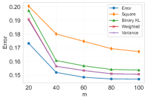
(a) Task size $n=2$

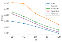
(b) Task size $n=3$

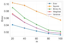
(c) Task size $n=4$

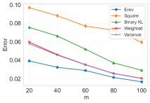
(d) Task size $n=5$

Figure 1: Comparison of the meta-generalization bounds on synthetic Gaussian datasets.

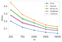
(a) MNIST, Adam ($n=10$)

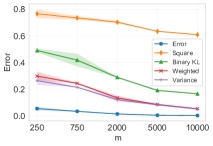
(b) MNIST, SGLD ($n=10$)

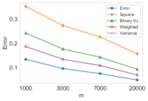
(c) CIFAR-10, SGD ($n=10$)

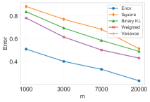
(d) CIFAR-10, SGLD ($n=10$)

Figure 2: Comparison of the meta-generalization bounds on real-world datasets with different optimizers.

5 Numerical Results

This section evaluates the validity and enhancements of theoretical results by empirically comparing the generalization gap and its various upper bounds. We focus on the loss-based bounds developed in Section 3, including the binary KL bound (Theorem 3.12), the square-root bound (Theorem 3.15), and the fast-rate bounds (Theorems 3.16 and 3.18). The binary loss function is adopted in the experiments to quantify the empirical and population risks. To precisely quantify the derived bounds, the experimental setup is consistent with previous work Wang & Mao (2023).

5.1 Synthetic Datasets

Our initial experiment considers $n$-class classification tasks within meta-learning settings, where each class containing $m$ training samples is regarded as a meta-learning training task. We follow the experimental details outlined in Wang & Mao (2023) to generalize synthetic Gaussian data for each task. Figure 1 plots the generalization gap and the corresponding generalization bounds on synthetic Gaussian datasets trained using a simple MLP network with MAML algorithms. As shown in Figure 1, our bounds adeptly adapt to varying numbers $n$ of meta-training tasks and sizes $m$ of per-task samples, coinciding well with the convergence trend of meta-generalization gap: the bounds decrease as $n\times m$ increases. A comparison among these bounds illustrates that the fast-rate bounds serve as the most stringent estimation of the generalization gap.

5.2 Real-world Datasets

We further extend the experimental analysis to deep-learning scenarios on real-world datasets. We employ a 4-layer MLP network trained on the MNIST dataset and a pre-trained ResNet-$50$ network with the CIFAR-10 dataset. Figure 2 demonstrates the closeness of the generalization gap to various bounds, exhibiting the same trend regrading the size of the training dataset. Notably, the weighted and loss variance bounds have shown to be the tightest among the upper bounds, aligning with the analysis of their stringency.

6 Conclusion

This paper provides a unified generalization analysis for meta-learning by developing various information-theoretic bounds. Theoretical results improve upon existing bounds in terms of tightness, scaling rate, and computational feasibility. Our analysis is modular and broadly applicable to a wide range of meta-learning methods. Numerical results also demonstrate a strong correlation between the true generalization gap and the derived bounds.

Appendix A Preparatory Definitions and Lemmas

Definition A.1 ($\sigma$-sub-gaussian).

A random variable $X$ is $\sigma$-sub-gaussian if for any $\lambda$, $\ln\mathbb{E}[e^{\lambda(X-\mathbb{E}X)}]\leq\lambda^{2}\sigma^{2}/2$.

Definition A.2 (Binary Relative Entropy).

Let $p,q\in[0,1]$. Then $d(p\|q)$ denotes the relative entropy between two Bernoulli random variables with parameters $p$ and $q$ respectively, defined as $d(p\|q)=p\log(\frac{p}{q})+(1-p)\log(\frac{1-p}{1-q})$. Given $\gamma\in\mathbb{R}$, $d_{\gamma}(p\|q)=\gamma p-\log(1-q+qe^{\gamma})$ is the relaxed version of binary relative entropy. One can prove that $\sup_{\gamma}d_{\gamma}(p\|q)=d(p\|q)$.

Definition A.3 (Kullback-Leibler Divergence).

Let $P$ and $Q$ be probability distributions defined on the same measurable space such that $P$ is absolutely continuous with respect to $Q$. The Kullback-Leibler (KL) divergence between $P$ and $Q$ is defined as $D(P\|Q)\triangleq\int_{\mathcal{X}}p(x)\log(\frac{p(x)}{q(x)})dx$.

Definition A.4 (Mutual Information).

For random variables $X$ and $Y$ with joint distribution $P_{X,Y}$ and product of their marginals $P_{X}P_{Y}$, the mutual information between $X$ and $Y$ is defined as $I(X;Y)=D(P_{X,Y}\|P_{X}P_{Y})$.

Lemma A.5 (Donsker-Varadhan Formula (Theorem 5.2.1 in Gray (2011))).

Let $P$ and $Q$ be probability measures over the same space $\mathcal{X}$ such that $P$ is absolutely continuous with respect to $Q$. For any bounded function $f:\mathcal{X}\rightarrow\mathbb{R}$,

$$D(P\|Q)=\sup_{f}\Big{\{}\mathbb{E}_{X\sim P}[f(X)]-\log\mathbb{E}_{X\sim Q}[e^{f(X)}]\Big{\}},$$

where $X$ is any random variable such that both $\mathbb{E}_{X\sim P}[f(X)]$ and $\mathbb{E}_{X\sim Q}[e^{f(X)}]$ exist.

Lemma A.6 (Lemma 1 in Harutyunyan et al. (2021)).

Let $(X,Y)$ be a pair of random variables with joint distribution $P_{X,Y}$, and $\bar{Y}$ be an independent copy of $Y$. If $f(x,y)$ be a measurable function such that $\mathbb{E}_{X,Y}[f(X,Y)]$ exists and $\mathbb{E}_{X,\bar{Y}}[f(X,\bar{Y})]$ is $\sigma$-sub-gaussian, then

$$\big{|}\mathbb{E}_{X,Y}[f(X,Y)]-\mathbb{E}_{X,\bar{Y}}[f(X,\bar{Y})]\big{|}\leq\sqrt{2\sigma^{2}I(X,Y)}.$$

Lemma A.7 (Lemma 3 in Harutyunyan et al. (2021)).

Let $X$ and $Y$ be independent random variables. If $f$ is a measurable function such that $f(x,Y)$ is $\sigma$-sub-gaussian and $\mathbb{E}f(x,Y)=0$ for all $x\in\mathcal{X}$, then $f(X,Y)$ is also $\sigma$-sub-gaussian.

Lemma A.8 (Lemma 2 in Hellström & Durisi (2022a)).

Let $X_{1},\ldots,X_{n}$ be $n$ independent random variables that for $i\in[n]$, $X_{i}\sim P_{X_{i}}$, $\mathbb{E}[X_{i}]=\mu_{i}$, $\bar{\mu}=\frac{1}{n}\sum_{i=1}^{n}X_{i}$, and $\mu=\frac{1}{n}\sum_{i=1}^{n}\mu_{i}$. Assume that $X_{i}\in[0,1]$ almost surely. Then, for any $\gamma>0$, $\mathbb{E}[e^{(nd_{\gamma}(\bar{\mu}\|\mu))}]\leq 1$.

Lemma A.9 (Lemma A.11 in Dong et al. (2024)).

Let $X\sim N(0,\Sigma)$ and $Y$ be any zero-mean random vector satisfying $\mathrm{Cov}_{Y}[Y]=\Sigma$, then $H(Y)\leq H(X)$.

Lemma A.10 (Lemma 9 in Dong et al. (2023)).

For any symmetric positive-definite matrix $A$, let $A=\Big{[}\begin{matrix}B&D^{T}\\ D&C\end{matrix}\Big{]}$ be a partition of $A$, where $B$ and $C$ are square matrices, then $|A|\leq|B||C|$.

Appendix B Omitted Proofs [Input-Output MI Bounds]

B.1 Proof of Theorem 3.2

Theorem 3.2 (Restate).

Let $\mathbb{K}$ and $\mathbb{J}$ be random subsets of $[n]$ and $[m]$ with sizes $\zeta$ and $\xi$, respectively, independent of $T^{\mathbb{N}}_{\mathbb{M}}$ and $(U,W_{\mathbb{N}})$. Assume that $\ell(U,W,Z)$ is $\sigma$-sub-gaussian for all $Z\sim P_{Z|\tau},\tau\sim P_{\mathcal{T}}$, $U\in\mathcal{U},W\in\mathcal{W}$, then

$$|\overline{\mathrm{gen}}|\leq\mathbb{E}_{K\sim\mathbb{K},J\sim\mathbb{J}}\sqrt{\frac{2\sigma^{2}}{\zeta\xi}I(U,W_{K};T^{K}_{J})}.$$

Proof.

Let random subsets $\mathbb{K},\mathbb{J}$ be fixed to $\mathbb{K}=K,\mathbb{J}=J$ with size $\zeta$ and $\xi$, and independent of $(U,W_{\mathbb{N}})$ and $T^{\mathbb{N}}_{\mathbb{M}}$. Let $\tau_{K}=\{\tau_{i}\}_{i\in K}$, $T^{K}_{J}=\{Z^{i}_{j}\}_{i\in K,j\in J}\subseteq T^{\mathbb{N}}_{\mathbb{M}}$, $W_{K}=\{W_{i}\}_{i\in K}$, and

$$f(U,W_{K},T^{K}_{J})=\frac{1}{\zeta}\sum_{i\in K}\frac{1}{\xi}\sum_{j\in J}\ell(U,W_{i},Z^{i}_{j}).$$

Let $\bar{U}$ and $\bar{T}^{\mathbb{N}}_{\mathbb{M}}$ be independent copy of $U$ and $T^{\mathbb{N}}_{\mathbb{M}}$. Applying Lemma A.5 with $P=P_{\tau_{K},T^{K}_{J}}P_{U|T^{K}_{J}}P_{W_{K}|U,T^{K}_{J}}$, $Q=P_{\tau_{K},T^{K}_{J}}P_{\bar{U}}P_{W|U,T^{K}_{J}}P_{\bar{T}^{K}_{J}|\tau_{K}}$, and $f=f(U,W_{K},T^{K}_{J})$, we get that

$$D(P_{\tau_{K},T^{K}_{J}}P_{U|T^{K}_{J}}P_{W_{K}|U,T^{K}_{J}}\|P_{\tau_{K},T^{K}_{J}}P_{\bar{U}}P_{W|U,T^{K}_{J}}P_{\bar{T}^{K}_{J}|\tau_{K}})$$

$$\geq \sup_{\lambda}\Big{\{}\lambda\Big{(}\mathbb{E}_{\tau_{K},T^{K}_{J},U,W_{K}}[f(U,W_{K},T^{K}_{J})]-\mathbb{E}_{\tau_{K},T^{K}_{J}}\mathbb{E}_{\bar{U},\bar{T}^{K}_{J}|\tau_{K}}\mathbb{E}_{W|U,T^{K}_{J}}[f(\bar{U},W_{K},\bar{T}^{K}_{J})]\Big{)}$$

$$-\log\mathbb{E}_{\tau_{K},T^{K}_{J}}\mathbb{E}_{\bar{U},\bar{T}^{K}_{J}|\tau_{K}}\mathbb{E}_{W|U,T^{K}_{J}}\Big{[}e^{\lambda\big{(}f(\bar{U},W_{K},\bar{T}^{K}_{J})-\mathbb{E}[f(\bar{U},W_{K},\bar{T}^{K}_{J})]\big{)}}\Big{]}\Big{\}},$$ (4)

where

$$D(P_{\tau_{K},T^{K}_{J}}P_{U|T^{K}_{J}}P_{W_{K}|U,T^{K}_{J}}\|P_{\tau_{K},T^{K}_{J}}P_{\bar{U}}P_{W|U,T^{K}_{J}}P_{\bar{T}^{K}_{J}|\tau_{K}})$$

$$= D(P_{\tau_{K},T^{K}_{J}}P_{U|T^{K}_{J}}\|P_{\bar{U}}P_{\bar{T}^{K}_{J}|\tau_{K}})+D(P_{W_{K}|U,T^{K}_{J}}\|P_{\bar{W}_{K}|U,\tau_{K}}|P_{\tau_{K},T^{K}_{J}}P_{U})$$

$$= I(U;T^{K}_{J})+I(W_{K};T^{K}_{J}|\tau_{K},U)$$ (5)

By the sub-gaussian property of the loss function, it is clear that the random variable $f(\bar{U},W_{K},\bar{T}^{K}_{J})$ is $\frac{\sigma}{\sqrt{\zeta\xi}}$-sub-gaussian, which implies that

$$\log\mathbb{E}_{\tau_{K},T^{K}_{J}}\mathbb{E}_{\bar{U},\bar{T}^{K}_{J}|\tau_{K}}\mathbb{E}_{W|U,T^{K}_{J}}\Big{[}e^{\lambda\big{(}f(\bar{U},W_{K},\bar{T}^{K}_{J})-\mathbb{E}[f(\bar{U},W_{K},\bar{T}^{K}_{J})]\big{)}}\Big{]}\leq\frac{\lambda^{2}\sigma^{2}}{2\xi\zeta}.$$

Putting the above back into (4) and combining with (5), we have

$$D(P_{\tau_{K},T^{K}_{J}}P_{U|T^{K}_{J}}P_{W_{K}|U,T^{K}_{J}}\|P_{\tau_{K},T^{K}_{J}}P_{\bar{U}}P_{W|U,T^{K}_{J}}P_{\bar{T}^{K}_{J}|\tau_{K}})$$

$$= I(U;T^{K}_{J})+I(W_{K};T^{K}_{J}|\tau_{K},U)$$

$$\geq \sup_{\lambda}\Big{\{}\lambda\Big{(}\mathbb{E}_{\tau_{K},T^{K}_{J},U,W_{K}}[f(U,W_{K},T^{K}_{J})]-\mathbb{E}_{\tau_{K},T^{K}_{J}}\mathbb{E}_{\bar{U},\bar{T}^{K}_{J}|\tau_{K}}\mathbb{E}_{W|U,T^{K}_{J}}[f(\bar{U},W_{K},\bar{T}^{K}_{J})]\Big{)}-\frac{\lambda^{2}\sigma^{2}}{2\xi\zeta}\Big{\}}.$$

Solving $\lambda$ to maximize the RHS of the above inequality, we get that

$$\Big{|}\mathbb{E}_{\tau_{K},T^{K}_{J},U,W_{K}}[f(U,W_{K},T^{K}_{J})]-\mathbb{E}_{\tau_{K},T^{K}_{J}}\mathbb{E}_{\bar{U},\bar{T}^{K}_{J}|\tau_{K}}\mathbb{E}_{W|U,T^{K}_{J}}[f(\bar{U},W_{K},\bar{T}^{K}_{J})]\Big{|}$$

$$= \bigg{|}\mathbb{E}_{\tau_{K},T^{K}_{J},U,W_{K}}\Big{[}\frac{1}{\zeta}\sum_{i\in K}\frac{1}{\xi}\sum_{j\in J}\ell(U,W_{i},Z^{i}_{j})\Big{]}-\mathbb{E}_{\tau_{K},T^{K}_{J}}\mathbb{E}_{\bar{U},\bar{T}^{K}_{J}|\tau_{K}}\mathbb{E}_{W|U,T^{K}_{J}}\Big{[}\frac{1}{\zeta}\sum_{i\in K}\frac{1}{\xi}\sum_{j\in J}\ell(\bar{U},W_{i},\bar{Z}^{i}_{j})\Big{]}\bigg{|}$$

$$\leq \sqrt{\frac{2\sigma^{2}}{\zeta\xi}\Big{(}I(U;T^{K}_{J})+I(W_{K};T^{K}_{J}|\tau_{K},U)\Big{)}}.$$

Taking expectation over $K,J$ on both sides and applying Jensen’s inequality on the absolute value function, we have

$$\bigg{|}\mathbb{E}_{K\sim\mathbb{K},J\sim\mathbb{J}}\bigg{[}\mathbb{E}_{\tau_{K},T^{K}_{J},U,W_{K}}\Big{[}\frac{1}{\zeta}\sum_{i\in K}\frac{1}{\xi}\sum_{j\in J}\ell(U,W_{i},Z^{i}_{j})\Big{]}-\mathbb{E}_{\tau_{K},T^{K}_{J}}\mathbb{E}_{\bar{U},\bar{T}^{K}_{J}|\tau_{K}}\mathbb{E}_{W|U,T^{K}_{J}}\Big{[}\frac{1}{\zeta}\sum_{i\in K}\frac{1}{\xi}\sum_{j\in J}\ell(\bar{U},W_{i},\bar{Z}^{i}_{j})\Big{]}\bigg{]}\bigg{|}$$

$$= \bigg{|}\mathbb{E}_{\tau_{\mathbb{N}},T^{\mathbb{N}}_{\mathbb{M}},U,W_{\mathbb{N}}}\Big{[}\frac{1}{nm}\sum_{i,j=1}^{n,m}\ell(U,W_{i},Z^{i}_{j})\Big{]}-\mathbb{E}_{\tau_{\mathbb{N}},T^{\mathbb{N}}_{\mathbb{M}}}\mathbb{E}_{\bar{U},\bar{T}^{\mathbb{N}}_{\mathbb{M}}|\tau_{\mathbb{N}}}\mathbb{E}_{W|U,T^{\mathbb{N}}_{\mathbb{M}}}\Big{[}\frac{1}{nm}\sum_{i,j=1}^{n,m}\ell(\bar{U},W_{i},\bar{Z}^{i}_{j})\Big{]}\bigg{|}$$

$$\leq \mathbb{E}_{K\sim\mathbb{K},J\sim\mathbb{J}}\sqrt{\frac{2\sigma^{2}}{\zeta\xi}\Big{(}I(U;T^{K}_{J})+I(W_{K};T^{K}_{J}|\tau_{K},U)\Big{)}}.$$ (6)

Notice that

$$I(W_{K};T^{K}_{J}|\tau_{K},U)\leq I(W_{K};T^{K}_{J}|\tau_{K},U)+I(W_{K};\tau_{K}|U)=I(W_{K};T^{K}_{J},\tau_{K}|U)=I(W_{K};T^{K}_{J}|U).$$

Putting the above inequality back into (6), we obtain that

$$\bigg{|}\mathbb{E}_{\tau_{\mathbb{N}},T^{\mathbb{N}}_{\mathbb{M}},U,W_{\mathbb{N}}}\Big{[}\frac{1}{nm}\sum_{i,j=1}^{n,m}\ell(U,W_{i},Z^{i}_{j})\Big{]}-\mathbb{E}_{\tau_{\mathbb{N}},T^{\mathbb{N}}_{\mathbb{M}}}\mathbb{E}_{\bar{U},\bar{T}^{\mathbb{N}}_{\mathbb{M}}|\tau_{\mathbb{N}}}\mathbb{E}_{W|U,T^{\mathbb{N}}_{\mathbb{M}}}\Big{[}\frac{1}{nm}\sum_{i,j=1}^{n,m}\ell(\bar{U},W_{i},\bar{Z}^{i}_{j})\Big{]}\bigg{|}$$

$$\leq \mathbb{E}_{K\sim\mathbb{K},J\sim\mathbb{J}}\sqrt{\frac{2\sigma^{2}}{\zeta\xi}\Big{(}I(U;T^{K}_{J})+I(W_{K};T^{K}_{J}|\tau_{K},U)\Big{)}}$$

$$\leq \mathbb{E}_{K\sim\mathbb{K},J\sim\mathbb{J}}\sqrt{\frac{2\sigma^{2}}{\zeta\xi}\Big{(}I(U;T^{K}_{J})+I(W_{K};T^{K}_{J}|U)\Big{)}}$$

$$= \mathbb{E}_{K\sim\mathbb{K},J\sim\mathbb{J}}\sqrt{\frac{2\sigma^{2}}{\zeta\xi}I(U,W_{K};T^{K}_{J})}.$$ (7)

We proceed to prove that the LSH of the inequality (7) is equivalent to the absolute value of the meta-generalization gap. Notice that $W_{i}$, $i=1,\ldots,n$ are mutually independent given $U$ and $T^{\mathbb{N}}_{\mathbb{M}}$, $P_{W_{\mathbb{N}}|U,T^{\mathbb{N}}_{\mathbb{M}}}=\prod_{i=1}^{n}P_{W_{i}|U,T^{i}_{\mathbb{M}}}$, we have

$$\mathbb{E}_{\tau_{\mathbb{N}},T^{\mathbb{N}}_{\mathbb{M}},U,W_{\mathbb{N}}}\bigg{[}\frac{1}{n}\sum_{i=1}^{n}\frac{1}{m}\sum_{j=1}^{m}\ell(U,W_{i},Z^{i}_{j})\bigg{]}= \mathbb{E}_{U,T^{\mathbb{N}}_{\mathbb{M}}}\bigg{[}\frac{1}{n}\sum_{i=1}^{n}\frac{1}{m}\sum_{j=1}^{m}\mathbb{E}_{W_{\mathbb{N}}|U,T^{\mathbb{N}}_{\mathbb{M}}}[\ell(U,W_{i},Z^{i}_{j})]\bigg{]}$$

$$= \mathbb{E}_{U,T^{\mathbb{N}}_{\mathbb{M}}}\bigg{[}\frac{1}{n}\sum_{i=1}^{n}\frac{1}{m}\sum_{j=1}^{m}\mathbb{E}_{W_{i}|U,T^{i}_{\mathbb{M}}}\ell(U,W_{i},Z^{i}_{j})\bigg{]}$$

$$= \mathbb{E}_{U,T^{\mathbb{N}}_{\mathbb{M}}}[\mathcal{R}(U,T^{\mathbb{N}}_{\mathbb{M}})].$$

For the second term on LSH of the inequality (7), we have

$$\mathbb{E}_{\tau_{\mathbb{N}},T^{\mathbb{N}}_{\mathbb{M}}}\mathbb{E}_{\bar{U}}\mathbb{E}_{W|U,T^{\mathbb{N}}_{\mathbb{M}}}\mathbb{E}_{\bar{T}^{\mathbb{N}}_{\mathbb{M}}|\tau_{\mathbb{N}}}\Big{[}\frac{1}{n}\sum_{i=1}^{n}\frac{1}{m}\sum_{j=1}^{m}\ell(\bar{U},W_{i},\bar{Z}^{i}_{j})\Big{]}= \mathbb{E}_{\bar{U},T^{\mathbb{N}}_{\mathbb{M}}}\bigg{[}\frac{1}{n}\sum_{i=1}^{n}\frac{1}{m}\sum_{j=1}^{m}\mathbb{E}_{W_{\mathbb{N}}|U,T^{\mathbb{N}}_{\mathbb{M}}}\mathbb{E}_{\tau_{\mathbb{N}}}\mathbb{E}_{\bar{T}^{\mathbb{N}}_{\mathbb{M}}|\tau_{\mathbb{N}}}\ell(\bar{U},W_{i},\bar{Z}^{i}_{j})\bigg{]}$$

$$= \mathbb{E}_{\bar{U},T^{\mathbb{N}}_{\mathbb{M}}}\bigg{[}\frac{1}{n}\sum_{i=1}^{n}\mathbb{E}_{W_{i}|U,T^{i}_{\mathbb{M}}}\mathbb{E}_{\tau_{i}\sim P_{\mathcal{T}}}\mathbb{E}_{Z^{\prime}\sim P_{Z|\tau_{i}}}\ell(\bar{U},W_{i},Z^{\prime})\bigg{]}$$

$$= \mathbb{E}_{U,T^{\mathbb{N}}_{\mathbb{M}}}\bigg{[}\frac{1}{n}\sum_{i=1}^{n}\mathbb{E}_{W_{i}|\bar{U},T^{i}_{\mathbb{M}}}\mathbb{E}_{\tau_{i}\sim P_{\mathcal{T}}}\mathbb{E}_{Z^{\prime}\sim P_{Z|\tau_{i}}}\ell(U,W_{i},Z^{\prime})\bigg{]}$$

$$= \mathbb{E}_{U,T^{\mathbb{N}}_{\mathbb{M}}}\bigg{[}\frac{1}{n}\sum_{i=1}^{n}\mathbb{E}_{\tau_{i}\sim P_{\mathcal{T}}}\mathbb{E}_{\bar{T}^{i}_{\mathbb{M}}\sim P_{Z|\tau_{i}}}\mathbb{E}_{\bar{W}_{i}|U,\bar{T}^{i}_{\mathbb{M}}}\mathbb{E}_{Z^{\prime}\sim P_{Z|\tau_{i}}}\ell(U,\bar{W}_{i},Z^{\prime})\bigg{]}$$

$$= \mathbb{E}_{U,T^{\mathbb{N}}_{\mathbb{M}}}\bigg{[}\mathbb{E}_{\tau\sim P_{\mathcal{T}}}\mathbb{E}_{T_{\mathbb{M}}|\tau}\mathbb{E}_{W|U,T_{\mathbb{M}}}\mathbb{E}_{Z^{\prime}\sim P^{\prime}_{Z|\tau}}\ell(U,W,Z^{\prime})\bigg{]}$$

$$= \mathbb{E}_{U,T^{\mathbb{N}}_{\mathbb{M}}}[\mathcal{R}(U,\mathcal{T})].$$

Plugging the above estimations into (7), we obtain

$$\Big{|}\mathbb{E}_{U,T^{\mathbb{N}}_{\mathbb{M}}}[\mathcal{R}(U,T^{\mathbb{N}}_{\mathbb{M}})]-\mathbb{E}_{U,T^{\mathbb{N}}_{\mathbb{M}}}[\mathcal{R}(U,\mathcal{T})]\Big{|}\leq \mathbb{E}_{K\sim\mathbb{K},J\sim\mathbb{J}}\sqrt{\frac{2\sigma^{2}}{\zeta\xi}I(U,W_{K};T^{K}_{J})}.$$

This completes the proof.

∎

B.2 Proof of Proposition 3.3

Proposition 3.3 (Restate).

Let $\zeta\in[n-1]$, $\xi\in[m-1]$, and $\mathbb{K}$ and $\mathbb{J}$ be random subsets of $[n]$ and $[m]$ with sizes $\zeta$ and $\xi$, respectively. Further, let $\mathbb{K}^{\prime}$ and $\mathbb{J}^{\prime}$ be random subsets of $[n]$ and $[m]$ with sizes $\zeta+1$ and $\xi+1$, respectively. If $g:\mathbb{R}\rightarrow\mathbb{R}$ is any non-decreasing concave function, then

$$\mathbb{E}_{K\sim\mathbb{K},J\sim\mathbb{J}}g\left(\frac{1}{\zeta\xi}I(U,W_{K};T^{K}_{J})\right)\leq\mathbb{E}_{K^{\prime}\sim\mathbb{K}^{\prime},J^{\prime}\sim\mathbb{J}^{\prime}}g\left(\frac{1}{(\zeta+1)(\xi+1)}I(U,W_{K^{\prime}};T^{K^{\prime}}_{J^{\prime}})\right).$$

Proof.

Let subsets $K^{\prime}=(K^{\prime}_{1},\ldots,K^{\prime}_{\zeta+1})\sim\mathbb{K}^{\prime}\subseteq[n]$ and $J^{\prime}=(J^{\prime}_{1},\ldots,J^{\prime}_{\xi+1})\sim\mathbb{J}^{\prime}\subseteq[n]$. By applying the chain rule of MI, we have

$$I(U,W_{K^{\prime}};T^{K^{\prime}}_{J^{\prime}})=I(U;T^{K^{\prime}}_{J^{\prime}})+I(W_{K^{\prime}};T^{K^{\prime}}_{J^{\prime}}|U).$$

$$I(U;T^{K^{\prime}}_{J^{\prime}})= \sum_{i=1}^{\zeta+1}I(U;T^{K^{\prime}_{i}}_{J^{\prime}}|T^{K^{\prime}_{1:i-1}}_{J^{\prime}})$$

$$= \sum_{i=1}^{\zeta+1}I(U,T^{K^{\prime}_{i+1:\zeta+1}}_{J^{\prime}};T^{K^{\prime}_{i}}_{J^{\prime}}|T^{K^{\prime}_{1:i-1}}_{J^{\prime}})-I(T^{K^{\prime}_{i}}_{J^{\prime}};T^{K^{\prime}_{i+1:\zeta+1}}_{J^{\prime}}|U,T^{K^{\prime}_{1:i-1}}_{J^{\prime}})$$

$$= \sum_{i=1}^{\zeta+1}I(U,T^{K^{\prime}_{i+1:\zeta+1}}_{J^{\prime}};T^{K^{\prime}_{i}}_{J^{\prime}}|T^{K^{\prime}_{1:i-1}}_{J^{\prime}})$$

$$= \sum_{i=1}^{\zeta+1}I(U;T^{K^{\prime}_{i}}_{J^{\prime}}|T^{K^{\prime}_{i+1:\zeta+1}}_{J^{\prime}},T^{K^{\prime}_{1:i-1}}_{J^{\prime}})+I(T^{K^{\prime}_{i}}_{J^{\prime}};T^{K^{\prime}_{i+1:\zeta+1}}_{J^{\prime}}|T^{K^{\prime}_{1:i-1}}_{J^{\prime}})$$

$$= \sum_{i=1}^{\zeta+1}I(U;T^{K^{\prime}_{i}}_{J^{\prime}}|T^{K^{\prime}_{i+1:\zeta+1}}_{J^{\prime}},T^{K^{\prime}_{1:i-1}}_{J^{\prime}}).$$ (8)

Leveraging the inequality (8), we have

$$I(U;T^{K^{\prime}}_{J^{\prime}})= \frac{1}{\zeta+1}\sum_{K^{\prime}_{i}\in K^{\prime}}\big{(}I(U;T^{K^{\prime}\backslash K^{\prime}_{i}}_{J^{\prime}})+I(U;T^{K^{\prime}_{i}}_{J^{\prime}}|T^{K^{\prime}\backslash K^{\prime}_{i}}_{J^{\prime}})\big{)}\geq\frac{1}{\zeta+1}\Big{(}\sum_{K^{\prime}_{i}\in K^{\prime}}I(U;T^{K^{\prime}\backslash K^{\prime}_{i}}_{J^{\prime}})+I(U;T^{K^{\prime}}_{J^{\prime}})\Big{)}$$

$$\geq \frac{1}{\zeta}\sum_{K^{\prime}_{i}\in K^{\prime}}I(U;T^{K^{\prime}\backslash K^{\prime}_{i}}_{J^{\prime}}).$$ (9)

Let $T^{K^{\prime}\backslash K^{\prime}_{i}}_{J^{\prime}}=\{Z^{K^{\prime}\backslash K^{\prime}_{i}}_{J^{\prime}_{1}},\ldots,Z^{K^{\prime}\backslash K^{\prime}_{i}}_{J^{\prime}_{\xi+1}}\}$, where $Z^{K^{\prime}\backslash K^{\prime}_{i}}_{J^{\prime}_{j}}=\{Z^{K^{\prime}_{1}}_{J^{\prime}_{j}},\ldots,Z^{K^{\prime}_{i-1}}_{J^{\prime}_{j}},Z^{K^{\prime}_{i+1}}_{J^{\prime}_{j}},\ldots,Z^{K^{\prime}_{\zeta+1}}_{J^{\prime}_{j}}\}$ for $j\in[\xi+1]$. Again using the chain rule of MI on $I(U;T^{K^{\prime}\backslash K^{\prime}_{i}}_{J^{\prime}})$, we have

$$I(U;T^{K^{\prime}\backslash K^{\prime}_{i}}_{J^{\prime}})= \sum_{j=1}^{\xi+1}I(U;Z^{K^{\prime}\backslash K^{\prime}_{i}}_{J^{\prime}_{j}}|Z^{K^{\prime}\backslash K^{\prime}_{i}}_{J^{\prime}_{1:j-1}})$$

$$= \sum_{j=1}^{\xi+1}I(U,Z^{K^{\prime}\backslash K^{\prime}_{i}}_{J^{\prime}_{j+1:\xi+1}};Z^{K^{\prime}\backslash K^{\prime}_{i}}_{J^{\prime}_{j}}|Z^{K^{\prime}\backslash K^{\prime}_{i}}_{J^{\prime}_{1:j-1}})-\sum_{j=1}^{\xi+1}I(Z^{K^{\prime}\backslash K^{\prime}_{i}}_{J^{\prime}_{j+1:\xi+1}};Z^{K^{\prime}\backslash K^{\prime}_{i}}_{J^{\prime}_{j}}|U,Z^{K^{\prime}\backslash K^{\prime}_{i}}_{J^{\prime}_{1:j-1}})$$

$$= \sum_{j=1}^{\xi+1}I(U,Z^{K^{\prime}\backslash K^{\prime}_{i}}_{J^{\prime}_{j+1:\xi+1}};Z^{K^{\prime}\backslash K^{\prime}_{i}}_{J^{\prime}_{j}}|Z^{K^{\prime}\backslash K^{\prime}_{i}}_{J^{\prime}_{1:j-1}})$$

$$= \sum_{j=1}^{\xi+1}I(U;Z^{K^{\prime}\backslash K^{\prime}_{i}}_{J^{\prime}_{j}}|Z^{K^{\prime}\backslash K^{\prime}_{i}}_{J^{\prime}_{1:j-1}},Z^{K^{\prime}\backslash K^{\prime}_{i}}_{J^{\prime}_{j+1:\xi+1}})+\sum_{j=1}^{\xi+1}I(Z^{K^{\prime}\backslash K^{\prime}_{i}}_{J^{\prime}_{j+1:\xi+1}};Z^{K^{\prime}\backslash K^{\prime}_{i}}_{J^{\prime}_{j}}|Z^{K^{\prime}\backslash K^{\prime}_{i}}_{J^{\prime}_{1:j-1}})$$

$$= \sum_{j=1}^{\xi+1}I(U;Z^{K^{\prime}\backslash K^{\prime}_{i}}_{J^{\prime}_{j}}|Z^{K^{\prime}\backslash K^{\prime}_{i}}_{J^{\prime}_{1:j-1}},Z^{K^{\prime}\backslash K^{\prime}_{i}}_{J^{\prime}_{j+1:\xi+1}}).$$ (10)

Similarly, we obtain that

$$I(U;T^{K^{\prime}\backslash K^{\prime}_{i}}_{J^{\prime}})= \frac{1}{\xi+1}\sum_{J^{\prime}_{j}\in J^{\prime}}\big{(}I(U;T^{K^{\prime}\backslash K^{\prime}_{i}}_{J^{\prime}\backslash J^{\prime}_{j}})+I(U;Z^{K^{\prime}\backslash K^{\prime}_{i}}_{J^{\prime}_{j}}|T^{K^{\prime}\backslash K^{\prime}_{i}}_{J^{\prime}\backslash J^{\prime}_{j}})\big{)}$$

$$= \frac{1}{\xi+1}\sum_{J^{\prime}_{j}\in J^{\prime}}\big{(}I(U;T^{K^{\prime}\backslash K^{\prime}_{i}}_{J^{\prime}\backslash J^{\prime}_{j}})+I(U;Z^{K^{\prime}\backslash K^{\prime}_{i}}_{J^{\prime}_{j}}|Z^{K^{\prime}\backslash K^{\prime}_{i}}_{J^{\prime}_{1:j-1}},Z^{K^{\prime}\backslash K^{\prime}_{i}}_{J^{\prime}_{j+1:\xi+1}})\big{)}$$

$$\geq \frac{1}{\xi+1}\Big{(}\sum_{J^{\prime}_{j}\in J^{\prime}}I(U;T^{K^{\prime}\backslash K^{\prime}_{i}}_{J^{\prime}\backslash J^{\prime}_{j}})+I(U;T^{K^{\prime}\backslash K^{\prime}_{i}}_{J^{\prime}})\Big{)}$$

$$\geq \frac{1}{\xi}\sum_{J^{\prime}_{j}\in J^{\prime}}I(U;T^{K^{\prime}\backslash K^{\prime}_{i}}_{J^{\prime}\backslash J^{\prime}_{j}}).$$ (11)

Putting (11) back into (9) yields

$$I(U;T^{K^{\prime}}_{J^{\prime}})\geq\frac{1}{\zeta\xi}\sum_{K^{\prime}_{i}\in K^{\prime},J^{\prime}_{j}\in J^{\prime}}I(U;T^{K^{\prime}\backslash K^{\prime}_{i}}_{J^{\prime}\backslash J^{\prime}_{j}}).$$ (12)

Analogously analyzing $I(W_{K^{\prime}};T^{K^{\prime}}_{J^{\prime}}|U)$. Since $W_{i}$, $i=1,\ldots,n$ are mutually independent given $T^{\mathbb{N}}_{\mathbb{M}}$ and $U$, we get that

$$I(W_{K^{\prime}};T^{K^{\prime}}_{J^{\prime}}|,U)= \sum_{i=1}^{\zeta+1}I(W_{K^{\prime}};T^{K_{i}^{\prime}}_{J^{\prime}}|U,T^{K^{\prime}_{1:i-1}}_{J^{\prime}})$$

$$= \sum_{i=1}^{\zeta+1}I(W_{K^{\prime}},T^{K^{\prime}_{i+1:\zeta+1}}_{J^{\prime}};T^{K_{i}^{\prime}}_{J^{\prime}}|U,T^{K^{\prime}_{1:i-1}}_{J^{\prime}})-I(T^{K^{\prime}_{i+1:\zeta+1}}_{J^{\prime}};T^{K_{i}^{\prime}}_{J^{\prime}}|U,W_{K^{\prime}},T^{K^{\prime}_{1:i-1}}_{J^{\prime}})$$

$$= \sum_{i=1}^{\zeta+1}I(W_{K^{\prime}},T^{K^{\prime}_{i+1:\zeta+1}}_{J^{\prime}};T^{K_{i}^{\prime}}_{J^{\prime}}|U,T^{K^{\prime}_{1:i-1}}_{J^{\prime}})$$

$$= \sum_{i=1}^{\zeta+1}I(W_{K^{\prime}_{i}};T^{K_{i}^{\prime}}_{J^{\prime}}|U,T^{K^{\prime}_{1:i-1}}_{J^{\prime}},T^{K^{\prime}_{i+1:\zeta+1}}_{J^{\prime}})+I(T^{K^{\prime}_{i+1:\zeta+1}}_{J^{\prime}};T^{K_{i}^{\prime}}_{J^{\prime}}|U,T^{K^{\prime}_{1:i-1}}_{J^{\prime}})$$

$$= \sum_{i=1}^{\zeta+1}I(W_{K^{\prime}_{i}};T^{K_{i}^{\prime}}_{J^{\prime}}|U,T^{K^{\prime}_{1:i-1}}_{J^{\prime}},T^{K^{\prime}_{i+1:\zeta+1}}_{J^{\prime}}).$$ (13)

Using the inequality (13), we have

$$I(W_{K^{\prime}};T^{K^{\prime}}_{J^{\prime}}|U)= \frac{1}{\zeta+1}\sum_{K^{\prime}_{i}\in K^{\prime}}\big{(}I(W_{K^{\prime}\backslash K^{\prime}_{i}};T^{K^{\prime}\backslash K^{\prime}_{i}}_{J^{\prime}}|U)+I(W_{K^{\prime}_{i}};T^{K^{\prime}_{i}}_{J^{\prime}}|T^{K^{\prime}\backslash K^{\prime}_{i}}_{J^{\prime}},U)\big{)}$$

$$\geq \frac{1}{\zeta+1}\Big{(}\sum_{K^{\prime}_{i}\in K^{\prime}}I(W_{K^{\prime}\backslash K^{\prime}_{i}};T^{K^{\prime}\backslash K^{\prime}_{i}}_{J^{\prime}}|U)+I(W_{K^{\prime}};T^{K^{\prime}}_{J^{\prime}}|U)\Big{)}$$

$$\geq \frac{1}{\zeta}\sum_{K^{\prime}_{i}\in K^{\prime}}I(W_{K^{\prime}\backslash K^{\prime}_{i}};T^{K^{\prime}\backslash K^{\prime}_{i}}_{J^{\prime}}|U).$$ (14)

Similar to the proof of the inequality (10), for the RHS of (14), we further get that

$$I(W_{K^{\prime}\backslash K^{\prime}_{i}};T^{K^{\prime}\backslash K^{\prime}_{i}}_{J^{\prime}}|U)=\sum_{j=1}^{\xi+1}I(W_{K^{\prime}\backslash K^{\prime}_{i}};Z^{K^{\prime}\backslash K^{\prime}_{i}}_{J^{\prime}_{j}}|U,Z^{K^{\prime}\backslash K^{\prime}_{i}}_{J^{\prime}_{1:j-1}})\leq\sum_{j=1}^{\xi+1}I(W_{K^{\prime}\backslash K^{\prime}_{i}};Z^{K^{\prime}\backslash K^{\prime}_{i}}_{J^{\prime}_{j}}|U,Z^{K^{\prime}\backslash K^{\prime}_{i}}_{J^{\prime}_{1:j-1}},Z^{K^{\prime}\backslash K^{\prime}_{i}}_{J^{\prime}_{j+1:\xi+1}}),$$

which implies that

$$I(W_{K^{\prime}\backslash K^{\prime}_{i}};T^{K^{\prime}\backslash K^{\prime}_{i}}_{J^{\prime}}|U)= \frac{1}{\xi+1}\sum_{J^{\prime}_{j}\in J^{\prime}}\big{(}I(W_{K^{\prime}\backslash K^{\prime}_{i}};T^{K^{\prime}\backslash K^{\prime}_{i}}_{J^{\prime}\backslash J^{\prime}_{j}}|U)+I(W_{K^{\prime}\backslash K^{\prime}_{i}};Z^{K^{\prime}\backslash K^{\prime}_{i}}_{J^{\prime}_{j}}|U,T^{K^{\prime}\backslash K^{\prime}_{i}}_{J^{\prime}\backslash J^{\prime}_{j}})\big{)}$$

$$= \frac{1}{\xi+1}\sum_{J^{\prime}_{j}\in J^{\prime}}\big{(}I(W_{K^{\prime}\backslash K^{\prime}_{i}};T^{K^{\prime}\backslash K^{\prime}_{i}}_{J^{\prime}\backslash J^{\prime}_{j}}|U)+I(W_{K^{\prime}\backslash K^{\prime}_{i}};Z^{K^{\prime}\backslash K^{\prime}_{i}}_{J^{\prime}_{j}}|U,Z^{K^{\prime}\backslash K^{\prime}_{i}}_{J^{\prime}_{1:j-1}},Z^{K^{\prime}\backslash K^{\prime}_{i}}_{J^{\prime}_{j+1:\xi+1}})\big{)}$$

$$\geq \frac{1}{\xi+1}\Big{(}\sum_{J^{\prime}_{j}\in J^{\prime}}I(W_{K^{\prime}\backslash K^{\prime}_{i}};T^{K^{\prime}\backslash K^{\prime}_{i}}_{J^{\prime}\backslash J^{\prime}_{j}}|U)+I(W_{K^{\prime}\backslash K^{\prime}_{i}};T^{K^{\prime}\backslash K^{\prime}_{i}}_{J^{\prime}}|U)\Big{)}$$

$$\geq \frac{1}{\xi}\sum_{J^{\prime}_{j}\in J^{\prime}}I(W_{K^{\prime}\backslash K^{\prime}_{i}};T^{K^{\prime}\backslash K^{\prime}_{i}}_{J^{\prime}\backslash J^{\prime}_{j}}|U).$$ (15)

Combining (14) and (15), we get that

$$I(W_{K^{\prime}};T^{K^{\prime}}_{J^{\prime}}|U)\geq\frac{1}{\zeta\xi}\sum_{K^{\prime}_{i}\in K^{\prime},J^{\prime}_{j}\in J^{\prime}}I(W_{K^{\prime}\backslash K^{\prime}_{i}};T^{K^{\prime}\backslash K^{\prime}_{i}}_{J^{\prime}\backslash J^{\prime}_{j}}|U).$$ (16)

By using the inequalities (12) and (16), one can obtain that

$$I(U,W_{K^{\prime}};T^{K^{\prime}}_{J^{\prime}})=I(U;T^{K^{\prime}}_{J^{\prime}})+I(W_{K^{\prime}};T^{K^{\prime}}_{J^{\prime}}|U)\geq \frac{1}{\zeta\xi}\sum_{K^{\prime}_{i}\in K^{\prime},J^{\prime}_{j}\in J^{\prime}}\big{(}I(W_{K^{\prime}\backslash K^{\prime}_{i}};T^{K^{\prime}\backslash K^{\prime}_{i}}_{J^{\prime}\backslash J^{\prime}_{j}}|U)+I(U;T^{K^{\prime}\backslash K^{\prime}_{i}}_{J^{\prime}\backslash J^{\prime}_{j}})\big{)}$$

$$= \frac{1}{\zeta\xi}\sum_{K^{\prime}_{i}\in K^{\prime},J^{\prime}_{j}\in J^{\prime}}I(U,W_{K^{\prime}\backslash K^{\prime}_{i}};T^{K^{\prime}\backslash K^{\prime}_{i}}_{J^{\prime}\backslash J^{\prime}_{j}}).$$

We further employ the Jensen’s inequality on the concave function $g$ and have

$$g\Big{(}\frac{1}{(\zeta+1)(\xi+1)}I(U,W_{K^{\prime}};T^{K^{\prime}}_{J^{\prime}})\Big{)}\geq g\Big{(}\frac{1}{(\zeta+1)(\xi+1)}\Big{(}\frac{1}{\zeta\xi}\sum_{K^{\prime}_{i}\in K^{\prime},J^{\prime}_{j}\in J^{\prime}}I(U,W_{K^{\prime}\backslash K^{\prime}_{i}};T^{K^{\prime}\backslash K^{\prime}_{i}}_{J^{\prime}\backslash J^{\prime}_{j}})\Big{)}\Big{)}$$

$$\geq \frac{1}{(\zeta+1)(\xi+1)}\sum_{K^{\prime}_{i}\in K^{\prime},J^{\prime}_{j}\in J^{\prime}}g\Big{(}\frac{1}{\zeta\xi}I(U,W_{K^{\prime}\backslash K^{\prime}_{i}};T^{K^{\prime}\backslash K^{\prime}_{i}}_{J^{\prime}\backslash J^{\prime}_{j}})\Big{)}$$ (17)

Taking expectation over $K^{\prime}$ and $J^{\prime}$ on both sides of (17),

$$\mathbb{E}_{K^{\prime}\sim\mathbb{K}^{\prime},J^{\prime}\sim\mathbb{J}^{\prime}}g\Big{(}\frac{1}{(\zeta+1)(\xi+1)}I(U,W_{K^{\prime}};T^{K^{\prime}}_{J^{\prime}})\Big{)}\geq \mathbb{E}_{K^{\prime}\sim\mathbb{K}^{\prime},J^{\prime}\sim\mathbb{J}^{\prime}}\bigg{[}\frac{1}{(\zeta+1)(\xi+1)}\sum_{K^{\prime}_{i}\in K^{\prime},J^{\prime}_{j}\in J^{\prime}}g\Big{(}\frac{1}{\zeta\xi}I(U,W_{K^{\prime}\backslash K^{\prime}_{i}};T^{K^{\prime}\backslash K^{\prime}_{i}}_{J^{\prime}\backslash J^{\prime}_{j}})\Big{)}\bigg{]}$$

$$= \frac{1}{C_{n}^{\zeta}C_{m}^{\xi}}\sum_{K\in\mathbb{K},J\in\mathbb{J}}g\Big{(}\frac{1}{\zeta\xi}I(U,W_{K};T^{K}_{J})\Big{)}$$

$$= \mathbb{E}_{K\sim\mathbb{K},J\sim\mathbb{J}}g\Big{(}\frac{1}{\zeta\xi}I(U,W_{K};T^{K}_{J})\Big{)},$$

and this completes the proof. ∎

Appendix C Omitted Proofs [CMI Bounds]

C.1 Proof of Theorem 3.5

Theorem 3.5 (Restate).

Let $\mathbb{K}$ and $\mathbb{J}$ be random subsets of $[n]$ and $[m]$ with sizes $\zeta$ and $\xi$, respectively. If the loss function $\ell(\cdot,\cdot,\cdot)$ is bounded within $[0,1]$, then

$$|\overline{\mathrm{gen}}|\leq\mathbb{E}_{T_{2\mathbb{M}}^{2\mathbb{N}},K\sim\mathbb{K},J\sim\mathbb{J}}\sqrt{\frac{2}{\zeta\xi}I^{T_{2\mathbb{M}}^{2\mathbb{N}}}(U,W_{K};\tilde{S}_{K},S_{J})}.$$

Proof.

Let us condition on $\mathbb{K}=K$, $\mathbb{J}=J$, and $T_{2\mathbb{M}}^{2\mathbb{N}}$. Further let $\tilde{S}_{K}=\{\tilde{S}_{i}\}_{i\in K}\subseteq\tilde{S}_{\mathbb{N}}$, $S_{J}=\{S_{j}\}_{j\in J}\subseteq S_{\mathbb{M}}$, and

$$f(u,\omega_{K},\tilde{s}_{K},s_{J})=\frac{1}{\zeta}\sum_{i\in K}\frac{1}{\xi}\sum_{j\in J}\Big{(}\ell(u,\omega_{i},\tilde{Z}^{i,\tilde{s}_{i}}_{j,s_{j}})-\ell(u,\omega_{i},\tilde{Z}^{i,\bar{\tilde{s}}_{i}}_{j,\bar{s}_{j}})\Big{)}.$$

Let $\tilde{S}^{\prime}_{\mathbb{N}}$ and $S^{\prime}_{\mathbb{M}}$ be independent copies of $S_{\mathbb{M}}$ and $\tilde{S}_{\mathbb{N}}$, respectively. It is noteworthy that each summand of $f(u,\omega_{K},\tilde{S}^{\prime}_{K},S^{\prime}_{J})$ is a $1$-sub-gaussian random variable and has zero mean, as $\ell(\cdot,\cdot,\cdot)$ take values in $[0,1]$. Hence, $f(u,\omega_{K},\tilde{S}^{\prime}_{K},S^{\prime}_{J})$ is $\frac{1}{\sqrt{\zeta\xi}}$-sub-gaussian with $\mathbb{E}_{\tilde{S}^{\prime}_{\mathbb{N}},S^{\prime}_{\mathbb{M}}}[f(u,\omega_{K},\tilde{S}^{\prime}_{K},S^{\prime}_{J})]=0$. Following Lemma A.7 with $X=(U,W_{K})$ and $Y=(\tilde{S}^{\prime}_{K},S^{\prime}_{J})$, we get that $f(U,W_{K},\tilde{S}^{\prime}_{K},S^{\prime}_{J})$ is also zero-mean $\frac{1}{\sqrt{\zeta\xi}}$-sub-gaussian. We further apply Lemma A.6 with the choices $X=(U,W_{K})$, $Y=(\tilde{S}_{K},S_{J})$ and $f(X,Y)=f(U,W_{K},\tilde{S}_{K},S_{J})$, and have

$$\bigg{|}\mathbb{E}_{U,W_{\mathbb{N}},\tilde{S}_{\mathbb{N}},S_{\mathbb{M}}}\bigg{[}\frac{1}{\zeta}\sum_{i\in K}\frac{1}{\xi}\sum_{j\in J}\Big{(}\ell(U,W_{i},\tilde{Z}^{i,\tilde{S}_{i}}_{j,S_{j}})-\ell(U,W_{i},\tilde{Z}^{i,\bar{\tilde{S}}_{i}}_{j,\bar{S}_{j}})\Big{)}\bigg{]}\bigg{|}\leq\sqrt{\frac{2}{\zeta\xi}I^{T_{2\mathbb{M}}^{2\mathbb{N}}}(U,W_{K};\tilde{S}_{K},S_{J})}.$$

Taking expectation over $K$, $J$ and $T_{2\mathbb{M}}^{2\mathbb{N}}$ on both sides and applying Jensen’s inequality to swap the order of expectation and absolute value, we obtain

$$\bigg{|}\mathbb{E}_{T_{2\mathbb{M}}^{2\mathbb{N}},K\sim\mathbb{K},J\sim\mathbb{J},U,W_{\mathbb{N}},\tilde{S}_{\mathbb{N}},S_{\mathbb{M}}}\bigg{[}\frac{1}{\zeta}\sum_{i\in K}\frac{1}{\xi}\sum_{j\in J}\Big{(}\ell(U,W_{i},\tilde{Z}^{i,\tilde{S}_{i}}_{j,S_{j}})-\ell(U,W_{i},\tilde{Z}^{i,\bar{\tilde{S}}_{i}}_{j,\bar{S}_{j}})\Big{)}\bigg{]}\bigg{|}$$

$$\leq \mathbb{E}_{T_{2\mathbb{M}}^{2\mathbb{N}},K\sim\mathbb{K},J\sim\mathbb{J}}\sqrt{\frac{2}{\zeta\xi}I^{T_{2\mathbb{M}}^{2\mathbb{N}}}(U,W_{K};\tilde{S}_{K},S_{J})},$$ (18)

which reduces to

$$\bigg{|}\mathbb{E}_{T_{2\mathbb{M}}^{2\mathbb{N}},U,W_{\mathbb{N}},\tilde{S}_{\mathbb{N}},S_{\mathbb{M}}}\bigg{[}\frac{1}{nm}\sum_{i,j=1}^{n,m}\Big{(}\ell(U,W_{i},\tilde{Z}^{i,\tilde{S}_{i}}_{j,S_{j}})-\ell(U,W_{i},\tilde{Z}^{i,\bar{\tilde{S}}_{i}}_{j,\bar{S}_{j}})\Big{)}\bigg{]}\bigg{|}\leq\mathbb{E}_{T_{2\mathbb{M}}^{2\mathbb{N}},K\sim\mathbb{K},J\sim\mathbb{J}}\sqrt{\frac{2}{\zeta\xi}I^{T_{2\mathbb{M}}^{2\mathbb{N}}}(U,W_{K};\tilde{S}_{K},S_{J})},$$ (19)

We then prove the LSH of the inequality (19) is equal to the absolute value of the meta-generalization gap. Since $\tilde{S}_{\mathbb{N}}\perp\bar{\tilde{S}}_{\mathbb{N}}$ and $S_{\mathbb{M}}\perp\bar{S}_{\mathbb{M}}$, we have $T_{2\mathbb{M},S_{\mathbb{M}}}^{2\mathbb{N},\tilde{S}_{\mathbb{N}}}\perp T_{2\mathbb{M},\bar{S}_{\mathbb{M}}}^{2\mathbb{N},\tilde{S}_{\mathbb{N}}}\perp T_{2\mathbb{M},S_{\mathbb{M}}}^{2\mathbb{N},\bar{\tilde{S}}_{\mathbb{N}}}\perp T^{2\mathbb{N},\bar{\tilde{S}}_{\mathbb{N}}}_{2\mathbb{M},\bar{S}_{\mathbb{M}}}$ and $W_{i}$, $i=1,\ldots,n$ are mutually independent given $U$ and $T_{2\mathbb{M},S_{\mathbb{M}}}^{2\mathbb{N},\tilde{S}_{\mathbb{N}}}$. Then

$$\mathbb{E}_{T_{2\mathbb{M}}^{2\mathbb{N}},U,W_{\mathbb{N}},\tilde{S}_{\mathbb{N}},S_{\mathbb{M}}}\Big{[}\frac{1}{nm}\sum_{i,j=1}^{n,m}\ell(U,W_{i},\tilde{Z}^{i,\tilde{S}_{i}}_{j,S_{j}})\Big{]}= \mathbb{E}_{U,W_{\mathbb{N}},T_{2\mathbb{M},S_{\mathbb{M}}}^{2\mathbb{N},\tilde{S}_{\mathbb{N}}},T_{2\mathbb{M},\bar{S}_{\mathbb{M}}}^{2\mathbb{N},\tilde{S}_{\mathbb{N}}},T_{2\mathbb{M},S_{\mathbb{M}}}^{2\mathbb{N},\bar{\tilde{S}}_{\mathbb{N}}},T^{2\mathbb{N},\bar{\tilde{S}}_{\mathbb{N}}}_{2\mathbb{M},\bar{S}_{\mathbb{M}}}}\Big{[}\frac{1}{nm}\sum_{i,j=1}^{n,m}\ell(U,W_{i},\tilde{Z}^{i,\tilde{S}_{i}}_{j,S_{j}})\Big{]}$$

$$= \mathbb{E}_{U,W_{\mathbb{N}},T_{2\mathbb{M},S_{\mathbb{M}}}^{2\mathbb{N},\tilde{S}_{\mathbb{N}}}}\Big{[}\frac{1}{nm}\sum_{i,j=1}^{n,m}\ell(U,W_{i},\tilde{Z}^{i,\tilde{S}_{i}}_{j,S_{j}})\Big{]}$$

$$= \mathbb{E}_{U,T_{2\mathbb{M},S_{\mathbb{M}}}^{2\mathbb{N},\tilde{S}_{\mathbb{N}}}}\Big{[}\frac{1}{nm}\sum_{i,j=1}^{n,m}\mathbb{E}_{W_{\mathbb{N}}|T_{2\mathbb{M},S_{\mathbb{M}}}^{2\mathbb{N},\tilde{S}_{\mathbb{N}}},U}\ell(U,W_{i},\tilde{Z}^{i,\tilde{S}_{i}}_{j,S_{j}})\Big{]}$$

$$= \mathbb{E}_{U,T_{2\mathbb{M},S_{\mathbb{M}}}^{2\mathbb{N},\tilde{S}_{\mathbb{N}}}}\Big{[}\frac{1}{nm}\sum_{i,j=1}^{n,m}\mathbb{E}_{W_{i}|T_{2\mathbb{M},S_{\mathbb{M}}}^{i,\tilde{S}_{i}},U}\ell(U,W_{i},\tilde{Z}^{i,\tilde{S}_{i}}_{j,S_{j}})\Big{]}$$

$$= \mathbb{E}_{U,T_{\mathbb{M}}^{\mathbb{N}}}\Big{[}\frac{1}{nm}\sum_{i,j=1}^{n,m}\mathbb{E}_{W_{i}|T_{\mathbb{M}}^{i},U}\ell(U,W_{i},Z^{i}_{j})\Big{]}$$

$$= \mathbb{E}_{U,T_{\mathbb{M}}^{\mathbb{N}}}[\mathcal{R}(U,T_{\mathbb{M}}^{\mathbb{N}})].$$ (20)

Similarly, by using the independence of $T_{2\mathbb{M},S_{\mathbb{M}}}^{2\mathbb{N},\tilde{S}_{\mathbb{N}}},T_{2\mathbb{M},\bar{S}_{\mathbb{M}}}^{2\mathbb{N},\tilde{S}_{\mathbb{N}}},T_{2\mathbb{M},\bar{S}_{\mathbb{M}}}^{2\mathbb{N},\bar{\tilde{S}}_{\mathbb{N}}},T^{2\mathbb{N},\bar{\tilde{S}}_{\mathbb{N}}}_{2\mathbb{M},S_{\mathbb{M}}}$, we have $T^{2\mathbb{N},\bar{\tilde{S}}_{\mathbb{N}}}_{2\mathbb{M},S_{\mathbb{M}}}\perp T_{2\mathbb{M},\bar{S}_{\mathbb{M}}}^{2\mathbb{N},\bar{\tilde{S}}_{\mathbb{N}}}\perp(T_{2\mathbb{M},S_{\mathbb{M}}}^{2\mathbb{N},\tilde{S}_{\mathbb{N}}},U)$ and $W_{i}$, $i=1,\ldots,n$ are mutually independent given $U$ and $T^{2\mathbb{N},\bar{\tilde{S}}_{\mathbb{N}}}_{2\mathbb{M},S_{\mathbb{M}}}$. We then have

$$\mathbb{E}_{T_{2\mathbb{M}}^{2\mathbb{N}},U,W_{\mathbb{N}},\tilde{S}_{\mathbb{N}},S_{\mathbb{M}}}\Big{[}\frac{1}{nm}\sum_{i,j=1}^{n,m}\ell(U,W_{i},\tilde{Z}^{i,\bar{\tilde{S}}_{i}}_{j,\bar{S}_{j}})\Big{]}$$

$$= \mathbb{E}_{U,W_{\mathbb{N}},T_{2\mathbb{M},S_{\mathbb{M}}}^{2\mathbb{N},\tilde{S}_{\mathbb{N}}},T_{2\mathbb{M},\bar{S}_{\mathbb{M}}}^{2\mathbb{N},\tilde{S}_{\mathbb{N}}},T_{2\mathbb{M},\bar{S}_{\mathbb{M}}}^{2\mathbb{N},\bar{\tilde{S}}_{\mathbb{N}}},T^{2\mathbb{N},\bar{\tilde{S}}_{\mathbb{N}}}_{2\mathbb{M},S_{\mathbb{M}}}}\Big{[}\frac{1}{nm}\sum_{i,j=1}^{n,m}\ell(U,W_{i},\tilde{Z}^{i,\bar{\tilde{S}}_{i}}_{j,\bar{S}_{j}})\Big{]}$$

$$= \mathbb{E}_{U,T_{2\mathbb{M},S_{\mathbb{M}}}^{2\mathbb{N},\tilde{S}_{\mathbb{N}}}}\Big{[}\frac{1}{nm}\sum_{i,j=1}^{n,m}\mathbb{E}_{W_{\mathbb{N}},T^{2\mathbb{N},\bar{\tilde{S}}_{\mathbb{N}}}_{2\mathbb{M},S_{\mathbb{M}}}|U}\mathbb{E}_{T_{2\mathbb{M},\bar{S}_{\mathbb{M}}}^{2\mathbb{N},\bar{\tilde{S}}_{\mathbb{N}}}}\ell(U,W_{i},\tilde{Z}^{i,\bar{\tilde{S}}_{i}}_{j,\bar{S}_{j}})\Big{]}$$

$$= \mathbb{E}_{U,T_{2\mathbb{M},S_{\mathbb{M}}}^{2\mathbb{N},\tilde{S}_{\mathbb{N}}}}\Big{[}\frac{1}{nm}\sum_{i,j=1}^{n,m}\mathbb{E}_{T^{2\mathbb{N},\bar{\tilde{S}}_{\mathbb{N}}}_{2\mathbb{M},S_{\mathbb{M}}}}\mathbb{E}_{W_{\mathbb{N}}|U,T^{2\mathbb{N},\bar{\tilde{S}}_{\mathbb{N}}}_{2\mathbb{M},S_{\mathbb{M}}}}\mathbb{E}_{T_{2\mathbb{M},\bar{S}_{\mathbb{M}}}^{2\mathbb{N},\bar{\tilde{S}}_{\mathbb{N}}}}\ell(U,W_{i},\tilde{Z}^{i,\bar{\tilde{S}}_{i}}_{j,\bar{S}_{j}})\Big{]}$$

$$= \mathbb{E}_{U,T_{2\mathbb{M},S_{\mathbb{M}}}^{2\mathbb{N},\tilde{S}_{\mathbb{N}}}}\Big{[}\frac{1}{nm}\sum_{i,j=1}^{n,m}\mathbb{E}_{T^{i,\bar{\tilde{S}}_{i}}_{2\mathbb{M},S_{\mathbb{M}}}}\mathbb{E}_{W_{i}|U,T^{i,\bar{\tilde{S}}_{i}}_{2\mathbb{M},S_{\mathbb{M}}}}\mathbb{E}_{T^{i,\bar{\tilde{S}}_{i}}_{2\mathbb{M},\bar{S}_{\mathbb{M}}}}\ell(U,W_{i},\tilde{Z}^{i,\bar{\tilde{S}}_{i}}_{j,\bar{S}_{j}})\Big{]}$$

$$= \mathbb{E}_{U,T_{2\mathbb{M},S_{\mathbb{M}}}^{2\mathbb{N},\tilde{S}_{\mathbb{N}}}}\Big{[}\frac{1}{n}\sum_{i=1}^{n}\mathbb{E}_{\tau_{i}\sim P_{\mathcal{T}}}\mathbb{E}_{T^{i,\bar{\tilde{S}}_{i}}_{2\mathbb{M},S_{\mathbb{M}}}\sim P_{Z|\tau_{i}}}\mathbb{E}_{W_{i}|U,T^{i,\bar{\tilde{S}}_{i}}_{2\mathbb{M},S_{\mathbb{M}}}}\mathbb{E}_{Z^{\prime}\sim P_{Z|\tau_{i}}}\ell(U,W_{i},Z^{\prime})\Big{]}$$

$$= \mathbb{E}_{U,T_{2\mathbb{M},S_{\mathbb{M}}}^{2\mathbb{N},\tilde{S}_{\mathbb{N}}}}\big{[}\mathbb{E}_{\tau\sim P_{\mathcal{T}}}\mathbb{E}_{T_{\mathbb{M}}\sim P_{Z|\tau}}\mathbb{E}_{W|U,T_{\mathbb{M}}}\mathbb{E}_{Z^{\prime}\sim P_{Z|\tau}}\ell(U,W,Z^{\prime})\big{]}$$

$$= \mathbb{E}_{U,T_{\mathbb{M}}^{\mathbb{N}}}[\mathcal{R}(U,\mathcal{T})]$$ (21)

Substituting (20) and (21) into (19), this completes the proof.

∎

C.2 Proof of Proposition 3.6

Proposition 3.6 (Restate).

Let $\zeta\in[n-1]$, $\xi\in[m-1]$, and $\mathbb{K}$ and $\mathbb{J}$ be random subsets of $[n]$ and $[m]$ with sizes $\zeta$ and $\xi$, respectively. Further, let $\mathbb{K}^{\prime}$ and $\mathbb{J}^{\prime}$ be random subsets with sizes $\zeta+1$ and $\xi+1$, respectively. If $g:\mathbb{R}\rightarrow\mathbb{R}$ is any non-decreasing concave function, then for $T_{2\mathbb{M}}^{2\mathbb{N}}\sim\{P_{Z|\tau_{i}}\}_{i=1}^{n}$ over $\mathcal{Z}^{2n\times 2m}$,

$$\mathbb{E}_{K\sim\mathbb{K},J\sim\mathbb{J}}g\left(\frac{1}{\zeta\xi}I^{T_{2\mathbb{M}}^{2\mathbb{N}}}(U,W_{K};\tilde{S}_{K},S_{J})\right)\leq\mathbb{E}_{K^{\prime}\sim\mathbb{K}^{\prime},J^{\prime}\sim\mathbb{J}^{\prime}}g\left(\frac{1}{(\zeta+1)(\xi+1)}I^{T_{2\mathbb{M}}^{2\mathbb{N}}}(U,W_{K^{\prime}};\tilde{S}_{K^{\prime}},S_{J^{\prime}})\right).$$

Proof.

The proof follows the same procedure as the proof of Proposition 3.3, by replacing the MI $I(U,W_{K};T^{K}_{J})$ with the disintegrated MI $I^{T_{2\mathbb{M}}^{2\mathbb{N}}}(U,W_{K};\tilde{S}_{K},S_{J})$. ∎

C.3 Proof of Theorem 3.7

Theorem 3.7 (Restate).

Assume that the loss function $\ell(\cdot,\cdot,\cdot)$ is bounded within $[0,1]$, then

$$d\left(\hat{\mathcal{R}}\Big{\|}\frac{\hat{\mathcal{R}}+\mathcal{R}_{\mathcal{T}}}{2}\right)\leq\frac{1}{nm}\sum_{i,j=1}^{n,m}I(U,W_{i};\tilde{S}_{i},S_{j}|T_{2\mathbb{M}}^{2\mathbb{N}}).$$

Furthermore, in the interpolating setting that $\hat{\mathcal{R}}=0$, we have

$$\mathcal{R}_{\mathcal{T}}\leq\frac{2}{nm}\sum_{i,j=1}^{n,m}I(U,W_{i};\tilde{S}_{i},S_{j}|T_{2\mathbb{M}}^{2\mathbb{N}}).$$

Proof.

Following the inequalities (20) and (21), we can decompose the average empirical and population risks into

$$\hat{\mathcal{R}}=\mathbb{E}_{T_{2\mathbb{M}}^{2\mathbb{N}},K\sim\mathbb{K},J\sim\mathbb{J},U,W_{\mathbb{N}},\tilde{S}_{\mathbb{N}},S_{\mathbb{M}}}\frac{1}{\zeta}\sum_{i\in K}\frac{1}{\xi}\sum_{j\in J}\ell(U,W_{i},\tilde{Z}^{i,\tilde{S}_{i}}_{j,S_{j}})$$ (22)

$$\mathcal{R}_{\mathcal{T}}=\mathbb{E}_{T_{2\mathbb{M}}^{2\mathbb{N}},K\sim\mathbb{K},J\sim\mathbb{J},U,W_{\mathbb{N}},\tilde{S}_{\mathbb{N}},S_{\mathbb{M}}}\frac{1}{\zeta}\sum_{i\in K}\frac{1}{\xi}\sum_{j\in J}\ell(U,W_{i},\tilde{Z}^{i,\bar{\tilde{S}}_{i}}_{j,\bar{S}_{j}})$$ (23)

Applying Jensen’s inequality and the convexity of $d_{\gamma}(\cdot\|\cdot)$, we obtain

$$d\left(\hat{\mathcal{R}}\Big{\|}\frac{\hat{\mathcal{R}}+\mathcal{R}_{\mathcal{T}}}{2}\right)$$

$$= \sup_{\gamma}d_{\gamma}\left(\hat{\mathcal{R}}\Big{\|}\frac{\hat{\mathcal{R}}+\mathcal{R}_{\mathcal{T}}}{2}\right)$$

$$\leq \sup_{\gamma}\frac{1}{\zeta\xi}\mathbb{E}_{K\sim\mathbb{K},J\sim\mathbb{J},T_{2\mathbb{M}}^{2\mathbb{N}},U,W_{\mathbb{N}},\tilde{S}_{\mathbb{N}},S_{\mathbb{M}}}d_{\gamma}\Bigg{(}\sum_{i\in K,j\in J}\ell(U,W_{i},\tilde{Z}^{i,\tilde{S}_{i}}_{j,S_{j}})\bigg{\|}\sum_{i\in K,j\in J}\frac{\ell(U,W_{i},\tilde{Z}^{i,\tilde{S}_{i}}_{j,S_{j}})+\ell(U,W_{i},\tilde{Z}^{i,\bar{\tilde{S}}_{i}}_{j,\bar{S}_{j}})}{2}\Bigg{)}$$

$$= \sup_{\gamma}\frac{1}{\zeta\xi}\mathbb{E}_{K\sim\mathbb{K},J\sim\mathbb{J},T_{2\mathbb{M}}^{2\mathbb{N}}}\mathbb{E}_{U,W_{K},\tilde{S}_{K},S_{J}|T_{2\mathbb{M}}^{2\mathbb{N}}}d_{\gamma}\Bigg{(}\sum_{i\in K,j\in J}\ell(U,W_{i},\tilde{Z}^{i,\tilde{S}_{i}}_{j,S_{j}})\bigg{\|}\sum_{i\in K,j\in J}\frac{\ell(U,W_{i},\tilde{Z}^{i,\tilde{S}_{i}}_{j,S_{j}})+\ell(U,W_{i},\tilde{Z}^{i,\bar{\tilde{S}}_{i}}_{j,\bar{S}_{j}})}{2}\Bigg{)}.$$ (24)

Let $\tilde{S}^{\prime}_{\mathbb{N}}$ and $S^{\prime}_{\mathbb{M}}$ be independent copies of $S_{\mathbb{M}}$ and $\tilde{S}_{\mathbb{N}}$. Let us condition on $K,J,T_{2\mathbb{M}}^{2\mathbb{N}}$ and utilize Lemma A.5 with $P=P_{U,W_{K},\tilde{S}_{K},S_{J}|T_{2\mathbb{M}}^{2\mathbb{N}}}$, $Q=P_{U,W_{K}|T_{2\mathbb{M}}^{2\mathbb{N}}}P_{\tilde{S}_{K},S_{J}}$, and $f=d_{\gamma}\Big{(}\sum_{i\in K,j\in J}\ell(U,W_{i},\tilde{Z}^{i,\tilde{S}_{i}}_{j,S_{j}})\Big{\|}\sum_{i\in K,j\in J}\frac{\ell(U,W_{i},\tilde{Z}^{i,\tilde{S}_{i}}_{j,S_{j}})+\ell(U,W_{i},\tilde{Z}^{i,\bar{\tilde{S}}_{i}}_{j,\bar{S}_{j}})}{2}\Big{)}$, we have

$$I^{T_{2\mathbb{M}}^{2\mathbb{N}}}(U,W_{K};\tilde{S}_{K},S_{J})= D\left(P_{U,W_{K},\tilde{S}_{K},S_{J}|T_{2\mathbb{M}}^{2\mathbb{N}}}\|P_{U,W_{K}|T_{2\mathbb{M}}^{2\mathbb{N}}}P_{\tilde{S}_{K},S_{J}}\right)$$

$$\geq \mathbb{E}_{U,W_{K},\tilde{S}_{K},S_{J}|T_{2\mathbb{M}}^{2\mathbb{N}}}d_{\gamma}\Bigg{(}\sum_{i\in K,j\in J}\ell(U,W_{i},\tilde{Z}^{i,\tilde{S}_{i}}_{j,S_{j}})\bigg{\|}\sum_{i\in K,j\in J}\frac{\ell(U,W_{i},\tilde{Z}^{i,\tilde{S}_{i}}_{j,S_{j}})+\ell(U,W_{i},\tilde{Z}^{i,\bar{\tilde{S}}_{i}}_{j,\bar{S}_{j}})}{2}\Bigg{)}$$

$$-\log\mathbb{E}_{U,W_{K},\tilde{S}^{\prime}_{K},S^{\prime}_{J}|T_{2\mathbb{M}}^{2\mathbb{N}}}e^{d_{\gamma}\Big{(}\sum_{i\in K,j\in J}\ell\big{(}U,W_{i},\tilde{Z}^{i,\tilde{S}^{\prime}_{i}}_{j,S^{\prime}_{j}}\big{)}\Big{\|}\sum_{i\in K,j\in J}\frac{\ell\big{(}U,W_{i},\tilde{Z}^{i,\tilde{S}^{\prime}_{i}}_{j,S^{\prime}_{j}}\big{)}+\ell\big{(}U,W_{i},\tilde{Z}^{i,\bar{\tilde{S}}^{\prime}_{i}}_{j,\bar{S}^{\prime}_{j}}\big{)}}{2}\Big{)}}.$$ (25)

Notice that

$$\mathbb{E}_{\tilde{S}^{\prime}_{K},S^{\prime}_{J}}\Big{[}\sum_{i\in K,j\in J}\ell\big{(}U,W_{i},\tilde{Z}^{i,\tilde{S}^{\prime}_{i}}_{j,S^{\prime}_{j}}\big{)}\Big{]}=\sum_{i\in K,j\in J}\mathbb{E}_{\tilde{S}^{\prime}_{i},S^{\prime}_{j}}\big{[}\ell\big{(}U,W_{i},\tilde{Z}^{i,\tilde{S}^{\prime}_{i}}_{j,S^{\prime}_{j}}\big{)}\big{]}=\sum_{i\in K,j\in J}\frac{\ell\big{(}U,W_{i},\tilde{Z}^{i,\tilde{S}^{\prime}_{i}}_{j,S^{\prime}_{j}}\big{)}+\ell\big{(}U,W_{i},\tilde{Z}^{i,\bar{\tilde{S}}^{\prime}_{i}}_{j,\bar{S}^{\prime}_{j}}\big{)}}{2}.$$

Utilizing Lemma A.8 and the above equation, for any $\gamma>0$, we know that

$$\mathbb{E}_{U,W_{K},\tilde{S}^{\prime}_{K},S^{\prime}_{J}|T_{2\mathbb{M}}^{2\mathbb{N}}}e^{d_{\gamma}\Big{(}\sum_{i\in K,j\in J}\ell\big{(}U,W_{i},\tilde{Z}^{i,\tilde{S}^{\prime}_{i}}_{j,S^{\prime}_{j}}\big{)}\Big{\|}\sum_{i\in K,j\in J}\frac{\ell\big{(}U,W_{i},\tilde{Z}^{i,\tilde{S}^{\prime}_{i}}_{j,S^{\prime}_{j}}\big{)}+\ell\big{(}U,W_{i},\tilde{Z}^{i,\bar{\tilde{S}}^{\prime}_{i}}_{j,\bar{S}^{\prime}_{j}}\big{)}}{2}\Big{)}}\leq 1.$$ (26)

Putting inequality (26) back into (25), we have

$$I^{T_{2\mathbb{M}}^{2\mathbb{N}}}(U,W_{K};\tilde{S}_{K},S_{J})\geq\mathbb{E}_{U,W_{K},\tilde{S}_{K},S_{J}|T_{2\mathbb{M}}^{2\mathbb{N}}}d_{\gamma}\Bigg{(}\sum_{i\in K,j\in J}\ell(U,W_{i},\tilde{Z}^{i,\tilde{S}_{i}}_{j,S_{j}})\bigg{\|}\sum_{i\in K,j\in J}\frac{\ell(U,W_{i},\tilde{Z}^{i,\tilde{S}_{i}}_{j,S_{j}})+\ell(U,W_{i},\tilde{Z}^{i,\bar{\tilde{S}}_{i}}_{j,\bar{S}_{j}})}{2}\Bigg{)}.$$ (27)

Further plugging (27) back into (24), we have

$$d\left(\hat{\mathcal{R}}\Big{\|}\frac{\hat{\mathcal{R}}+\mathcal{R}_{\mathcal{T}}}{2}\right)$$

$$\leq \sup_{\gamma}\frac{1}{\zeta\xi}\mathbb{E}_{K\sim\mathbb{K},J\sim\mathbb{J},T_{2\mathbb{M}}^{2\mathbb{N}}}\mathbb{E}_{U,W_{K},\tilde{S}_{K},S_{J}|T_{2\mathbb{M}}^{2\mathbb{N}}}d_{\gamma}\Bigg{(}\sum_{i\in K,j\in J}\ell(U,W_{i},\tilde{Z}^{i,\tilde{S}_{i}}_{j,S_{j}})\bigg{\|}\sum_{i\in K,j\in J}\frac{\ell(U,W_{i},\tilde{Z}^{i,\tilde{S}_{i}}_{j,S_{j}})+\ell(U,W_{i},\tilde{Z}^{i,\bar{\tilde{S}}_{i}}_{j,\bar{S}_{j}})}{2}\Bigg{)}$$

$$\leq \mathbb{E}_{K\sim\mathbb{K},J\sim\mathbb{J},T_{2\mathbb{M}}^{2\mathbb{N}}}\frac{I^{T_{2\mathbb{M}}^{2\mathbb{N}}}(U,W_{K};\tilde{S}_{K},S_{J})}{\zeta\xi}=\mathbb{E}_{K\sim\mathbb{K},J\sim\mathbb{J}}\frac{I(U,W_{K};\tilde{S}_{K},S_{J}|T_{2\mathbb{M}}^{2\mathbb{N}})}{\zeta\xi}.$$

By taking $\zeta=\xi=1$,

$$d\left(\hat{\mathcal{R}}\Big{\|}\frac{\hat{\mathcal{R}}+\mathcal{R}_{\mathcal{T}}}{2}\right)\leq\frac{1}{nm}\sum_{i,j=1}^{n,m}I(U,W_{i};\tilde{S}_{i},S_{j}|T_{2\mathbb{M}}^{2\mathbb{N}}).$$

When $\hat{\mathcal{R}}=0$, we obtain

$$d\left(\hat{\mathcal{R}}\Big{\|}\frac{\hat{\mathcal{R}}+\mathcal{R}_{\mathcal{T}}}{2}\right)=d\left(0\Big{\|}\frac{\mathcal{R}_{\mathcal{T}}}{2}\right)\geq\frac{\mathcal{R}_{\mathcal{T}}}{2}.$$

This completes the proof.

∎

C.4 Proof of Theorem 3.8

Theorem 3.8 (Restate).

Assume that the loss function $\ell(\cdot,\cdot,\cdot)$ is bounded within $[0,1]$, then for any $0\leq C_{2}\leq\log 2$ and $C_{1}\geq-\frac{\log(2-e^{C_{2}})}{C_{2}}-1$,

$$\overline{\mathrm{gen}}\leq C_{1}\hat{\mathcal{R}}+\frac{1}{nm}\sum_{i,j=1}^{n,m}\frac{I(U,W_{i};\tilde{S}_{i},S_{j}|T_{2\mathbb{M}}^{2\mathbb{N}})}{C_{2}}.$$

In the interpolating setting, i.e., $\hat{\mathcal{R}}=0$, we have

$$\mathcal{R}_{\mathcal{T}}\leq\frac{1}{nm}\sum_{i,j=1}^{n,m}\frac{I(U,W_{i};\tilde{S}_{i},S_{j}|T_{2\mathbb{M}}^{2\mathbb{N}})}{\log 2}.$$

Proof.

According to the definition of meta-generalization gap, we have

$$\mathcal{R}_{\mathcal{T}}-(1+C_{1})\hat{\mathcal{R}}= \mathbb{E}_{T_{2\mathbb{M}}^{2\mathbb{N}},U,W_{\mathbb{N}},\tilde{S}_{\mathbb{N}},S_{\mathbb{M}}}\bigg{[}\frac{1}{nm}\sum_{i,j=1}^{n,m}\Big{(}\ell(U,W_{i},\tilde{Z}^{i,\bar{\tilde{S}}_{i}}_{j,\bar{S}_{j}})-(1+C_{1})\ell(U,W_{i},\tilde{Z}^{i,\tilde{S}_{i}}_{j,S_{j}})\Big{)}\bigg{]}$$

$$= \mathbb{E}_{T_{2\mathbb{M}}^{2\mathbb{N}}}\frac{1}{nm}\sum_{i,j=1}^{n,m}\bigg{[}\mathbb{E}_{U,W_{i},\tilde{S}_{i},S_{j}|T_{2\mathbb{M}}^{2\mathbb{N}}}\Big{(}\ell(U,W_{i},\tilde{Z}^{i,\bar{\tilde{S}}_{i}}_{j,\bar{S}_{j}})-(1+C_{1})\ell(U,W_{i},\tilde{Z}^{i,\tilde{S}_{i}}_{j,S_{j}})\Big{)}\bigg{]}.$$

$$= \mathbb{E}_{T_{2\mathbb{M}}^{2\mathbb{N}}}\frac{1}{nm}\sum_{i,j=1}^{n,m}\bigg{[}\mathbb{E}_{U,W_{i},\tilde{S}_{i},S_{j}|T_{2\mathbb{M}}^{2\mathbb{N}}}\Big{(}L^{i,\bar{\tilde{S}}_{i}}_{j,\bar{S}_{j}}-(1+C_{1})L^{i,\tilde{S}_{i}}_{j,S_{j}}\Big{)}\bigg{]}.$$ (28)

Let $\tilde{S}^{\prime}_{\mathbb{N}}$ and $S^{\prime}_{\mathbb{M}}$ be independent copies of $S_{\mathbb{M}}$ and $\tilde{S}_{\mathbb{N}}$, respectively. By leveraging Lemma A.5 with $P=P_{U,W_{i},\tilde{S}_{i},S_{j}|T_{2\mathbb{M}}^{2\mathbb{N}}},Q=P_{U,W_{i}|T_{2\mathbb{M}}^{2\mathbb{N}}}P_{\tilde{S}_{i},S_{j}}$, and $f(U,W_{i},\tilde{S}_{i},S_{j})=L^{i,\bar{\tilde{S}}_{i}}_{j,\bar{S}_{j}}-(1+C_{1})L^{i,\tilde{S}_{i}}_{j,S_{j}}$, we get that

$$I^{T_{2\mathbb{M}}^{2\mathbb{N}}}(U,W_{i};\tilde{S}_{i},S_{j})= D(P_{U,W_{i},\tilde{S}_{i},S_{j}|T_{2\mathbb{M}}^{2\mathbb{N}}}\|P_{U,W_{i}|T_{2\mathbb{M}}^{2\mathbb{N}}}P_{\tilde{S}_{i},S_{j}})$$

$$\geq \sup_{C_{2}>0}\Big{\{}\mathbb{E}_{U,W_{i},\tilde{S}_{i},S_{j}|T_{2\mathbb{M}}^{2\mathbb{N}}}\Big{[}C_{2}\big{(}L^{i,\bar{\tilde{S}}_{i}}_{j,\bar{S}_{j}}-(1+C_{1})L^{i,\tilde{S}_{i}}_{j,S_{j}}\big{)}\Big{]}-\log\mathbb{E}_{U,W_{i},\tilde{S}^{\prime}_{i},S^{\prime}_{j}|T_{2\mathbb{M}}^{2\mathbb{N}}}\Big{[}e^{C_{2}\big{(}L^{i,\bar{\tilde{S}}^{\prime}_{i}}_{j,\bar{S}^{\prime}_{j}}-(1+C_{1})L^{i,\tilde{S}^{\prime}_{i}}_{j,S^{\prime}_{j}}\big{)}}\Big{]}\Big{\}}$$

$$= \sup_{C_{2}>0}\Bigg{\{}\mathbb{E}_{U,W_{i},\tilde{S}_{i},S_{j}|T_{2\mathbb{M}}^{2\mathbb{N}}}\Big{[}C_{2}\big{(}L^{i,\bar{\tilde{S}}_{i}}_{j,\bar{S}_{j}}-(1+C_{1})L^{i,\tilde{S}_{i}}_{j,S_{j}}\big{)}\Big{]}$$

$$-\log\bigg{(}\mathbb{I}\{\tilde{S}_{i}\oplus S_{j}=0\}\frac{\mathbb{E}_{U,W_{i}|T_{2\mathbb{M}}^{\mathbb{N}}}\Big{[}e^{C_{2}\big{(}L^{i,1}_{j,1}-C_{2}(1+C_{1})L^{i,0}_{j,0}\big{)}}+e^{C_{2}\big{(}L^{i,0}_{j,0}-C_{2}(1+C_{1})L^{i,1}_{j,1}\big{)}}\Big{]}}{2}$$

$$+\mathbb{I}\{\tilde{S}_{i}\oplus S_{j}=1\}\frac{\mathbb{E}_{U,W_{i}|T_{2\mathbb{M}}^{\mathbb{N}}}\Big{[}e^{C_{2}\big{(}L^{i,1}_{j,0}-C_{2}(1+C_{1})L^{i,0}_{j,1}\big{)}}+e^{C_{2}\big{(}L^{i,0}_{j,1}-C_{2}(1+C_{1})L^{i,1}_{j,0}\big{)}}\Big{]}}{2}\bigg{)}\Bigg{\}}$$

$$= \sup_{C_{2}>0}\bigg{\{}\mathbb{E}_{U,W_{i},\tilde{S}_{i},S_{j}|T_{2\mathbb{M}}^{2\mathbb{N}}}\Big{[}C_{2}\big{(}L^{i,\bar{\tilde{S}}_{i}}_{j,\bar{S}_{j}}-(1+C_{1})L^{i,\tilde{S}_{i}}_{j,S_{j}}\big{)}\Big{]}$$

$$-\log\frac{\mathbb{E}_{U,W_{i}|T_{2\mathbb{M}}^{\mathbb{N}}}\Big{[}e^{C_{2}\big{(}L^{\Psi_{+}}_{i,j}-C_{2}(1+C_{1})L^{\Psi_{-}}_{i,j}\big{)}}+e^{C_{2}\big{(}L^{\Psi_{-}}_{i,j}-C_{2}(1+C_{1})L^{\Psi_{+}}_{i,j}\big{)}}\Big{]}}{2}\bigg{\}}$$ (29)

where $\mathbb{I}\{\cdot\}$ is the indicator function. Let $\lambda_{C_{1},C_{2}}=e^{C_{2}\big{(}L^{\Psi_{+}}_{i,j}-C_{2}(1+C_{1})L^{\Psi_{-}}_{i,j}\big{)}}+e^{C_{2}\big{(}L^{\Psi_{-}}_{i,j}-C_{2}(1+C_{1})L^{\Psi_{+}}_{i,j}\big{)}}$. We intend to select the values of $C_{1},C_{2}$ such that the $\log$ term of (29) is guaranteed to less than $0$, that is $\lambda_{C_{1},C_{2}}\leq 2$. By the convexity of exponential function, one could know that the maximum value of this term can be achieved at the endpoints of $L^{\Psi_{-}}_{i,j},L^{\Psi_{+}}_{i,j}\in[0,1]$. It is natural that

$$\lambda_{C_{1},C_{2}}=\left\{\begin{array}[]{ll}2&if\quad L^{\Psi_{+}}_{i,j}=L^{\Psi_{-}}_{i,j}=0,\\ 2e^{-C_{1}C_{2}}&if\quad L^{\Psi_{+}}_{i,j}=L^{\Psi_{-}}_{i,j}=1,\\ e^{C_{2}}+e^{-C_{2}(1+C_{1})}&if\quad L^{\Psi_{+}}_{i,j}=1,L^{\Psi_{-}}_{i,j}=0\;\textrm{or}\;L^{\Psi_{+}}_{i,j}=0,L^{\Psi_{-}}_{i,j}=1.\\ \end{array}\right.$$

For the case of $L^{\Psi_{+}}_{i,j}=1$ and $L^{\Psi_{-}}_{i,j}=0$ ( or $L^{\Psi_{+}}_{i,j}=0,L^{\Psi_{-}}_{i,j}=1$), it suffices to select a large enough $C_{1}\rightarrow\infty$ such that $\lambda_{C_{1},C_{2}}=e^{C_{2}}+e^{-C_{2}-C_{1}C_{2}}\leq 2$, which implies that $C_{2}\leq\log 2$ and $C_{1}\geq-\frac{\log(2-e^{C_{2}})}{C_{2}}+1$. By the above estimations, we obtain

$$\log\frac{\mathbb{E}_{U,W_{i}|T_{2\mathbb{M}}^{\mathbb{N}}}\Big{[}e^{C_{2}\big{(}L^{\Psi_{+}}_{i,j}-C_{2}(1+C_{1})L^{\Psi_{-}}_{i,j}\big{)}}+e^{C_{2}\big{(}L^{\Psi_{-}}_{i,j}-C_{2}(1+C_{1})L^{\Psi_{+}}_{i,j}\big{)}}\Big{]}}{2}\leq 0.$$ (30)

Plugging the inequality (30) back into (29),

$$I^{T_{2\mathbb{M}}^{2\mathbb{N}}}(U,W_{i};\tilde{S}_{i},S_{j})\geq \mathbb{E}_{U,W_{i},\tilde{S}_{i},S_{j}|T_{2\mathbb{M}}^{2\mathbb{N}}}\Big{[}C_{2}\big{(}L^{i,\bar{\tilde{S}}_{i}}_{j,\bar{S}_{j}}-(1+C_{1})L^{i,\tilde{S}_{i}}_{j,S_{j}}\big{)}\Big{]}.$$ (31)

Substituting (31) into (28), we have

$$\overline{\mathrm{gen}}= \mathcal{R}_{\mathcal{T}}-(1+C_{1})\hat{\mathcal{R}}+C_{1}\hat{\mathcal{R}}$$

$$\leq C_{1}\hat{\mathcal{R}}+\frac{1}{nm}\sum_{i,j=1}^{n,m}\mathbb{E}_{T_{2\mathbb{M}}^{2\mathbb{N}}}\Big{[}\frac{I^{T_{2\mathbb{M}}^{2\mathbb{N}}}(U,W_{i};\tilde{S}_{i},S_{j})}{C_{2}}\Big{]}$$

$$= C_{1}\hat{\mathcal{R}}+\frac{1}{nm}\sum_{i,j=1}^{n,m}\frac{I(U,W_{i};\tilde{S}_{i},S_{j}|T_{2\mathbb{M}}^{2\mathbb{N}})}{C_{2}}.$$

In the interpolating regime where $\hat{\mathcal{R}}=0$, by letting $C_{2}\rightarrow\log 2$ and $C_{1}\rightarrow\infty$, we have

$$\mathcal{R}_{\mathcal{T}}\leq\frac{1}{nm}\sum_{i,j=1}^{n,m}\frac{I(U,W_{i};\tilde{S}_{i},S_{j}|T_{2\mathbb{M}}^{2\mathbb{N}})}{\log 2}.$$

This completes the proof. ∎

Appendix D Omitted Proofs [E-CMI Bounds]

D.1 Proof of Theorem 3.10

Theorem 3.10.

Assume that the loss function $\ell(\cdot,\cdot,\cdot)\in[0,1]$, then

$$|\overline{\mathrm{gen}}|\leq\frac{1}{nm}\sum_{i,j=1}^{n,m}\mathbb{E}_{T^{2\mathbb{N}}_{2\mathbb{M}}}\sqrt{2I^{T^{2\mathbb{N}}_{2\mathbb{M}}}(L^{i}_{j};\tilde{S}_{i},S_{j})}.$$

Proof.

Notice that

$$|\overline{\mathrm{gen}}|= \bigg{|}\mathbb{E}_{U,W_{\mathbb{N}},T_{2\mathbb{M}}^{2\mathbb{N}},\tilde{S}_{\mathbb{N}},S_{\mathbb{M}}}\Big{[}\frac{1}{nm}\sum_{i,j=1}^{n,m}\Big{(}\ell(U,W_{i},\tilde{Z}^{i,\bar{\tilde{S}}_{i}}_{j,\bar{S}_{j}})-\ell(U,W_{i},\tilde{Z}^{i,\tilde{S}_{i}}_{j,S_{j}})\Big{)}\Big{]}\bigg{|}$$

$$\leq \mathbb{E}_{T_{2\mathbb{M}}^{2\mathbb{N}}}\bigg{|}\mathbb{E}_{U,W_{\mathbb{N}},\tilde{S}_{\mathbb{N}},S_{\mathbb{M}}|T_{2\mathbb{M}}^{2\mathbb{N}}}\Big{[}\frac{1}{nm}\sum_{i,j=1}^{n,m}\Big{(}\ell(U,W_{i},\tilde{Z}^{i,\bar{\tilde{S}}_{i}}_{j,\bar{S}_{j}})-\ell(U,W_{i},\tilde{Z}^{i,\tilde{S}_{i}}_{j,S_{j}})\Big{)}\Big{]}\bigg{|}$$

$$\leq \mathbb{E}_{T_{2\mathbb{M}}^{2\mathbb{N}}}\frac{1}{nm}\sum_{i,j=1}^{n,m}\bigg{|}\mathbb{E}_{U,W_{i},\tilde{S}_{i},S_{j}|T_{2\mathbb{M}}^{2\mathbb{N}}}\Big{[}\ell(U,W_{i},\tilde{Z}^{i,\bar{\tilde{S}}_{i}}_{j,\bar{S}_{j}})-\ell(U,W_{i},\tilde{Z}^{i,\tilde{S}_{i}}_{j,S_{j}})\Big{]}\bigg{|}$$

$$\leq \mathbb{E}_{T_{2\mathbb{M}}^{2\mathbb{N}}}\frac{1}{nm}\sum_{i,j=1}^{n,m}\Big{|}\mathbb{E}_{L^{i}_{j},\tilde{S}_{i},S_{j}|T_{2\mathbb{M}}^{2\mathbb{N}}}\Big{[}L^{i,\bar{\tilde{S}}_{i}}_{j,\bar{S}_{j}}-L^{i,\tilde{S}_{i}}_{j,S_{j}}\Big{]}\Big{|}.$$ (32)

By the assumption of the loss function, we have $L^{i,\bar{\tilde{S}}_{i}}_{j,\bar{S}_{j}}-L^{i,\tilde{S}_{i}}_{j,S_{j}}\in[-1,1]$, and thus $L^{i,\bar{\tilde{S}}_{i}}_{j,\bar{S}_{j}}-L^{i,\tilde{S}_{i}}_{j,S_{j}}$ is $1$-sub-gaussian. Let $\tilde{S}^{\prime}_{\mathbb{N}},S^{\prime}_{\mathbb{M}}$ be independent copies of $\tilde{S}_{\mathbb{N}},S_{\mathbb{M}}$. Applying Lemma A.5 with $P=P_{L^{i}_{j},\tilde{S}_{i},S_{j}|T_{2\mathbb{M}}^{2\mathbb{N}}}$, $Q=P_{L^{i}_{j}|T_{2\mathbb{M}}^{2\mathbb{N}}}P_{\tilde{S}_{i},S_{j}}$ and $f(L^{i}_{j},\tilde{S}_{i},S_{j})=L^{i,\bar{\tilde{S}}_{i}}_{j,\bar{S}_{j}}-L^{i,\tilde{S}_{i}}_{j,S_{j}}$, we have

$$\Big{|}\mathbb{E}_{L^{i}_{j},\tilde{S}_{i},S_{j}|T_{2\mathbb{M}}^{2\mathbb{N}}}\Big{[}L^{i,\bar{\tilde{S}}_{i}}_{j,\bar{S}_{j}}-L^{i,\tilde{S}_{i}}_{j,S_{j}}\Big{]}-\mathbb{E}_{L^{i}_{j},\tilde{S}^{\prime}_{i},S^{\prime}_{j}|T_{2\mathbb{M}}^{2\mathbb{N}}}\Big{[}L^{i,\bar{\tilde{S}}^{\prime}_{i}}_{j,\bar{S}^{\prime}_{j}}-L^{i,\tilde{S}^{\prime}_{i}}_{j,S^{\prime}_{j}}\Big{]}\Big{|}\leq\sqrt{2I^{T^{2\mathbb{N}}_{2\mathbb{M}}}(L^{i}_{j};\tilde{S}_{i},S_{j})}.$$ (33)

It is easy to prove that $\mathbb{E}_{L^{i}_{j},\tilde{S}^{\prime}_{i},S^{\prime}_{j}|T_{2\mathbb{M}}^{2\mathbb{N}}}\big{[}L^{i,\bar{\tilde{S}}^{\prime}_{i}}_{j,\bar{S}^{\prime}_{j}}-L^{i,\tilde{S}^{\prime}_{i}}_{j,S^{\prime}_{j}}\big{]}=0$. Putting the above estimation back into (32), we obtain

$$|\overline{\mathrm{gen}}|\leq\frac{1}{nm}\sum_{i,j=1}^{n,m}\mathbb{E}_{T^{2\mathbb{N}}_{2\mathbb{M}}}\sqrt{2I^{T^{2\mathbb{N}}_{2\mathbb{M}}}(L^{i}_{j};\tilde{S}_{i},S_{j})},$$

and complete the proof. ∎

D.2 Proof of Theorem 3.11

Theorem 3.11.

Assume that the loss function $\ell(\cdot,\cdot,\cdot)\in[0,1]$, then

$$|\overline{\mathrm{gen}}|\leq\frac{1}{nm}\sum_{i,j=1}^{n,m}\sqrt{2I(L^{i}_{j};\tilde{S}_{i},S_{j})}.$$

Proof.

In the proof of Theorem 3.10, we notice that if we do not move the expectation over $T^{2\mathbb{N}}_{2\mathbb{M}}$ outside of the absolute function and directly take the expectation over $L^{i}_{j}$, we will have the opportunity to get rid of the expectation over $T^{2\mathbb{N}}_{2\mathbb{M}}$. By the definition of the meta-generalization gap, we get

$$|\overline{\mathrm{gen}}|= \bigg{|}\mathbb{E}_{U,W_{\mathbb{N}},T_{2\mathbb{M}}^{2\mathbb{N}},\tilde{S}_{\mathbb{N}},S_{\mathbb{M}}}\Big{[}\frac{1}{nm}\sum_{i,j=1}^{n,m}\Big{(}\ell(U,W_{i},\tilde{Z}^{i,\bar{\tilde{S}}_{i}}_{j,\bar{S}_{j}})-\ell(U,W_{i},\tilde{Z}^{i,\tilde{S}_{i}}_{j,S_{j}})\Big{)}\Big{]}\bigg{|}$$

$$= \Big{|}\frac{1}{nm}\sum_{i,j=1}^{n,m}\mathbb{E}_{T_{2\mathbb{M}}^{2\mathbb{N}},U,W_{i},\tilde{S}_{i},S_{j}}\Big{[}\ell(U,W_{i},\tilde{Z}^{i,\bar{\tilde{S}}_{i}}_{j,\bar{S}_{j}})-\ell(U,W_{i},\tilde{Z}^{i,\tilde{S}_{i}}_{j,S_{j}})\Big{]}\Big{|}$$

$$\leq \frac{1}{nm}\sum_{i,j=1}^{n,m}\Big{|}\mathbb{E}_{L^{i}_{j},\tilde{S}_{i},S_{j}}\Big{[}\ell(U,W_{i},\tilde{Z}^{i,\bar{\tilde{S}}_{i}}_{j,\bar{S}_{j}})-\ell(U,W_{i},\tilde{Z}^{i,\tilde{S}_{i}}_{j,S_{j}})\Big{]}\Big{|}$$

$$= \frac{1}{nm}\sum_{i,j=1}^{n,m}\Big{|}\mathbb{E}_{L^{i}_{j},\tilde{S}_{i},S_{j}}\Big{[}L^{i,\bar{\tilde{S}}_{i}}_{j,\bar{S}_{j}}-L^{i,\tilde{S}_{i}}_{j,S_{j}}\Big{]}\Big{|}.$$ (34)

Analogous proof to the inequality (33), we can similarly prove that

$$\Big{|}\mathbb{E}_{L^{i}_{j},\tilde{S}_{i},S_{j}}\Big{[}L^{i,\bar{\tilde{S}}_{i}}_{j,\bar{S}_{j}}-L^{i,\tilde{S}_{i}}_{j,S_{j}}\Big{]}-\mathbb{E}_{L^{i}_{j},\tilde{S}^{\prime}_{i},S^{\prime}_{j}}\Big{[}L^{i,\bar{\tilde{S}}^{\prime}_{i}}_{j,\bar{S}^{\prime}_{j}}-L^{i,\tilde{S}^{\prime}_{i}}_{j,S^{\prime}_{j}}\Big{]}\Big{|}\leq\sqrt{2I(L^{i}_{j};\tilde{S}_{i},S_{j})},$$

and $\mathbb{E}_{L^{i}_{j},\tilde{S}^{\prime}_{i},S^{\prime}_{j}}\big{[}L^{i,\bar{\tilde{S}}^{\prime}_{i}}_{j,\bar{S}^{\prime}_{j}}-L^{i,\tilde{S}^{\prime}_{i}}_{j,S^{\prime}_{j}}\big{]}=0$. Substituting the above inequality into (34) yields

$$|\overline{\mathrm{gen}}|\leq\frac{1}{nm}\sum_{i,j=1}^{n,m}\sqrt{2I(L^{i}_{j};\tilde{S}_{i},S_{j})},$$

which completes the proof. ∎

D.3 Proof of Theorem 3.12

Theorem 3.12.

Assume that the loss function $\ell(\cdot,\cdot,\cdot)\in[0,1]$, then

$$d\left(\hat{\mathcal{R}}\Big{\|}\frac{\hat{\mathcal{R}}+\mathcal{R}_{\mathcal{T}}}{2}\right)\leq\frac{1}{nm}\sum_{i,j=1}^{n,m}I(L^{i}_{j};\tilde{S}_{i},S_{j}).$$

Proof.

Recall that in (24), we have

$$d\left(\hat{\mathcal{R}}\Big{\|}\frac{\hat{\mathcal{R}}+\mathcal{R}_{\mathcal{T}}}{2}\right)\leq \sup_{\gamma}\frac{1}{nm}\mathbb{E}_{U,W_{\mathbb{N}},T_{2\mathbb{M}}^{2\mathbb{N}},\tilde{S}_{\mathbb{N}},S_{\mathbb{M}}}d_{\gamma}\Bigg{(}\sum_{i,j=1}^{n,m}\ell(U,W_{i},\tilde{Z}^{i,\tilde{S}_{i}}_{j,S_{j}})\bigg{\|}\sum_{i,j=1}^{n,m}\frac{\ell(U,W_{i},\tilde{Z}^{i,\tilde{S}_{i}}_{j,S_{j}})+\ell(U,W_{i},\tilde{Z}^{i,\bar{\tilde{S}}_{i}}_{j,\bar{S}_{j}})}{2}\Bigg{)}$$

$$\leq \sup_{\gamma}\frac{1}{nm}\sum_{i,j=1}^{n,m}\mathbb{E}_{U,W_{i},\tilde{S}_{i},S_{j},T_{2\mathbb{M}}^{2\mathbb{N}}}d_{\gamma}\Bigg{(}\ell(U,W_{i},\tilde{Z}^{i,\tilde{S}_{i}}_{j,S_{j}})\bigg{\|}\frac{\ell(U,W_{i},\tilde{Z}^{i,\tilde{S}_{i}}_{j,S_{j}})+\ell(U,W_{i},\tilde{Z}^{i,\bar{\tilde{S}}_{i}}_{j,\bar{S}_{j}})}{2}\Bigg{)}$$

$$= \sup_{\gamma}\frac{1}{nm}\sum_{i,j=1}^{n,m}\mathbb{E}_{L^{i}_{j},\tilde{S}_{i},S_{j}}d_{\gamma}\bigg{(}L^{i,\tilde{S}_{i}}_{j,S_{j}}\bigg{\|}\frac{L^{i,\tilde{S}_{i}}_{j,S_{j}}+L^{i,\bar{\tilde{S}}_{i}}_{j,\bar{S}_{j}}}{2}\bigg{)}.$$ (35)

Let $\tilde{S}^{\prime}_{\mathbb{N}},S^{\prime}_{\mathbb{M}}$ be independent copies of $\tilde{S}_{\mathbb{N}},S_{\mathbb{M}}$. Applying Lemma A.5 with $P=P_{L^{i}_{j},\tilde{S}_{i},S_{j}}$, $Q=P_{L_{j}^{i}}P_{\tilde{S}_{i},S_{j}}$, and $f(L^{i}_{j},\tilde{S}_{i},S_{j})=d_{\gamma}\big{(}L^{i,\tilde{S}_{i}}_{j,S_{j}}\big{\|}\frac{L^{i,\tilde{S}_{i}}_{j,S_{j}}+L^{i,\bar{\tilde{S}}_{i}}_{j,\bar{S}_{j}}}{2}\big{)}$, we have for any $\gamma>0$

$$I(L^{i}_{j};\tilde{S}_{i},S_{j})= D(P_{L^{i}_{j},\tilde{S}_{i},S_{j}}\|P_{L_{j}^{i}}P_{\tilde{S}_{i},S_{j}})$$

$$\geq \mathbb{E}_{L^{i}_{j},\tilde{S}_{i},S_{j}}d_{\gamma}\bigg{(}L^{i,\tilde{S}_{i}}_{j,S_{j}}\bigg{\|}\frac{L^{i,\tilde{S}_{i}}_{j,S_{j}}+L^{i,\bar{\tilde{S}}_{i}}_{j,\bar{S}_{j}}}{2}\bigg{)}-\log\mathbb{E}_{L^{i}_{j},\tilde{S}^{\prime}_{i},S^{\prime}_{j}}\bigg{[}e^{d_{\gamma}\Big{(}L^{i,\tilde{S}^{\prime}_{i}}_{j,S^{\prime}_{j}}\Big{\|}\frac{L^{i,\tilde{S}^{\prime}_{i}}_{j,S^{\prime}_{j}}+L^{i,\bar{\tilde{S}}^{\prime}_{i}}_{j,\bar{S}^{\prime}_{j}}}{2}\Big{)}}\bigg{]}.$$ (36)

Notice that $\mathbb{E}_{\tilde{S}^{\prime}_{i},S^{\prime}_{j}}[L^{i,\tilde{S}^{\prime}_{i}}_{j,S^{\prime}_{j}}]=(L^{i,\tilde{S}^{\prime}_{i}}_{j,S^{\prime}_{j}}+L^{i,\bar{\tilde{S}}^{\prime}_{i}}_{j,\bar{S}^{\prime}_{j}})/2$, by Lemma A.8, for any $\gamma\in\mathbb{R}$, we have

$$\mathbb{E}_{L^{i}_{j},\tilde{S}^{\prime}_{i},S^{\prime}_{j}}\bigg{[}e^{d_{\gamma}\Big{(}L^{i,\tilde{S}^{\prime}_{i}}_{j,S^{\prime}_{j}}\Big{\|}\frac{L^{i,\tilde{S}^{\prime}_{i}}_{j,S^{\prime}_{j}}+L^{i,\bar{\tilde{S}}^{\prime}_{i}}_{j,\bar{S}^{\prime}_{j}}}{2}\Big{)}}\bigg{]}\leq 1.$$

Plugging the above inequality into (36) implies that

$$\mathbb{E}_{L^{i}_{j},\tilde{S}_{i},S_{j}}d_{\gamma}\bigg{(}L^{i,\tilde{S}_{i}}_{j,S_{j}}\bigg{\|}\frac{L^{i,\tilde{S}_{i}}_{j,S_{j}}+L^{i,\bar{\tilde{S}}_{i}}_{j,\bar{S}_{j}}}{2}\bigg{)}\leq I(L^{i}_{j};\tilde{S}_{i},S_{j}).$$ (37)

Substituting (37) into (35), we have

$$d\left(\hat{\mathcal{R}}\Big{\|}\frac{\hat{\mathcal{R}}+\mathcal{R}_{\mathcal{T}}}{2}\right)\leq\frac{1}{nm}\sum_{i,j=1}^{n,m}I(L^{i}_{j};\tilde{S}_{i},S_{j}),$$

and complete the proof.

∎

Appendix E Omitted Proofs [Loss-difference Bounds]

E.1 Proof of Theorem 3.13

Theorem 3.13.

Assume that the loss function $\ell(\cdot,\cdot,\cdot)\in[0,1]$, then

$$|\overline{\mathrm{gen}}|\leq\frac{1}{nm}\sum_{i,j=1}^{n,m}\sqrt{2I(\Delta_{i,j}^{\Psi};S_{j}|T_{2\mathbb{M}}^{2\mathbb{N}})}.$$

Proof.

By the definition of the meta-generalization gap, we have

$$|\overline{\mathrm{gen}}|= \Big{|}\mathbb{E}_{U,W_{\mathbb{N}},T_{2\mathbb{M}}^{2\mathbb{N}},\tilde{S}_{\mathbb{N}},S_{\mathbb{M}}}\Big{[}\frac{1}{nm}\sum_{i,j=1}^{n,m}\Big{(}\ell(U,W_{i},\tilde{Z}^{i,\bar{\tilde{S}}_{i}}_{j,\bar{S}_{j}})-\ell(U,W_{i},\tilde{Z}^{i,\tilde{S}_{i}}_{j,S_{j}})\Big{)}\Big{]}\Big{|}$$

$$\leq \mathbb{E}_{T_{2\mathbb{M}}^{2\mathbb{N}}}\Big{|}\mathbb{E}_{L_{2\mathbb{M}}^{2\mathbb{N}},\tilde{S}_{\mathbb{N}},S_{\mathbb{M}}|T_{2\mathbb{M}}^{2\mathbb{N}}}\Big{[}\frac{1}{nm}\sum_{i,j=1}^{n,m}\Big{(}L^{i,\bar{\tilde{S}}_{i}}_{j,\bar{S}_{j}}-L^{i,\tilde{S}_{i}}_{j,S_{j}}\Big{)}\Big{]}\Big{|}$$

$$\leq \frac{1}{nm}\sum_{i,j=1}^{n,m}\mathbb{E}_{T_{2\mathbb{M}}^{2\mathbb{N}}}\Big{|}\mathbb{E}_{L^{i}_{j},\tilde{S}_{i},S_{j}|T_{2\mathbb{M}}^{2\mathbb{N}}}\big{[}\mathbb{I}\{\tilde{S}_{i}\oplus S_{j}=0\}(-1)^{S_{j}}(L^{i,1}_{j,1}-L^{i,0}_{j,0})+\mathbb{I}\{\tilde{S}_{i}\oplus S_{j}=1\}(-1)^{S_{j}}(L^{i,0}_{j,1}-L^{i,1}_{j,0})\big{]}\Big{|}$$

$$= \frac{1}{nm}\sum_{i,j=1}^{n,m}\mathbb{E}_{T_{2\mathbb{M}}^{2\mathbb{N}}}\Big{|}\mathbb{E}_{L_{i,j}^{\Psi},\tilde{S}_{i},S_{j}|T_{2\mathbb{M}}^{2\mathbb{N}}}\Big{[}(-1)^{S_{j}}\Big{(}L_{i,j}^{\Psi_{+}}-L_{i,j}^{\Psi_{-}}\Big{)}\Big{]}\Big{|}$$

$$= \frac{1}{nm}\sum_{i,j=1}^{n,m}\mathbb{E}_{T_{2\mathbb{M}}^{2\mathbb{N}}}\Big{|}\mathbb{E}_{\Delta_{i,j}^{\Psi},S_{j}|T_{2\mathbb{M}}^{2\mathbb{N}}}\big{[}(-1)^{S_{j}}\Delta_{i,j}^{\Psi}\big{]}\Big{|},$$ (38)

where $\mathbb{I}\{\cdot\}$ is the indicator function and the inequalities follows from the Jensen’s inequality on the absolute function. Since the loss function takes values in $[0,1]$, $\Delta_{i,j}^{\Psi}\in[-1,+1]$ and thus $(-1)^{S^{\prime}_{j}}\Delta_{i,j}^{\Psi}$ is $1$-sub-gaussian. Let $S^{\prime}_{\mathbb{M}}$ be an independent copy of $S_{\mathbb{M}}$. Applying Lemma A.5 with $P=P_{\Delta_{i,j}^{\Psi},S_{j}|T_{2\mathbb{M}}^{2\mathbb{N}}}$, $Q=P_{\Delta_{i,j}^{\Psi}|T_{2\mathbb{M}}^{2\mathbb{N}}}P_{S_{j}}$ and $f(\Delta_{i,j}^{\Psi},S_{j})=(-1)^{S_{j}}\Delta_{i,j}^{\Psi}$, we have

$$\Big{|}\mathbb{E}_{\Delta_{i,j}^{\Psi},S_{j}|T_{2\mathbb{M}}^{2\mathbb{N}}}\big{[}(-1)^{S_{j}}\Delta_{i,j}^{\Psi}\big{]}-\mathbb{E}_{\Delta_{i,j}^{\Psi},S^{\prime}_{j}|T_{2\mathbb{M}}^{2\mathbb{N}}}\big{[}(-1)^{S^{\prime}_{j}}\Delta_{i,j}^{\Psi}\big{]}\Big{|}=\Big{|}\mathbb{E}_{\Delta_{i,j}^{\Psi},S_{j}|T_{2\mathbb{M}}^{2\mathbb{N}}}\big{[}(-1)^{S_{j}}\Delta_{i,j}^{\Psi}\big{]}\Big{|}\leq\sqrt{2I^{T_{2\mathbb{M}}^{2\mathbb{N}}}(\Delta_{i,j}^{\Psi};S_{j})},$$

by $\mathbb{E}_{\Delta_{i,j}^{\Psi},S^{\prime}_{j}|T_{2\mathbb{M}}^{2\mathbb{N}}}\big{[}(-1)^{S^{\prime}_{j}}\Delta_{i,j}^{\Psi}\big{]}=0$. By substituting the above inequality into (38), we get that

$$|\overline{\mathrm{gen}}|\leq \frac{1}{nm}\sum_{i,j=1}^{n,m}\mathbb{E}_{T_{2\mathbb{M}}^{2\mathbb{N}}}\Big{|}\mathbb{E}_{\Delta_{i,j}^{\Psi},S_{j}|T_{2\mathbb{M}}^{2\mathbb{N}}}\big{[}(-1)^{S_{j}}\Delta_{i,j}^{\Psi}\big{]}\Big{|}\leq\frac{1}{nm}\sum_{i,j=1}^{n,m}\mathbb{E}_{T_{2\mathbb{M}}^{2\mathbb{N}}}\sqrt{2I^{T_{2\mathbb{M}}^{2\mathbb{N}}}(\Delta_{i,j}^{\Psi};S_{j})}$$

$$\leq \frac{1}{nm}\sum_{i,j=1}^{n,m}\sqrt{2I(\Delta_{i,j}^{\Psi};S_{j}|T_{2\mathbb{M}}^{2\mathbb{N}})}.$$

This completes the proof. ∎

E.2 Proof of Theorem 3.14

Theorem 3.14.

Assume that the loss function $\ell(\cdot,\cdot,\cdot)\in[0,1]$, then

$$|\overline{\mathrm{gen}}|\leq\frac{1}{nm}\sum_{i,j=1}^{n,m}\sqrt{2I(\Delta_{i,j}^{\Psi};S_{j})}.$$

Proof.

Notice that

$$|\overline{\mathrm{gen}}|= \Big{|}\mathbb{E}_{U,W_{\mathbb{N}},T_{2\mathbb{M}}^{2\mathbb{N}},\tilde{S}_{\mathbb{N}},S_{\mathbb{M}}}\Big{[}\frac{1}{nm}\sum_{i,j=1}^{n,m}\Big{(}\ell(U,W_{i},\tilde{Z}^{i,\bar{\tilde{S}}_{i}}_{j,\bar{S}_{j}})-\ell(U,W_{i},\tilde{Z}^{i,\tilde{S}_{i}}_{j,S_{j}})\Big{)}\Big{]}\Big{|}$$

$$= \Big{|}\mathbb{E}_{L_{2\mathbb{M}}^{2\mathbb{N}},\tilde{S}_{\mathbb{N}},S_{\mathbb{M}}}\Big{[}\frac{1}{nm}\sum_{i,j=1}^{n,m}\Big{(}L^{i,\bar{\tilde{S}}_{i}}_{j,\bar{S}_{j}}-L^{i,\tilde{S}_{i}}_{j,S_{j}}\Big{)}\Big{]}\Big{|}$$

$$\leq \frac{1}{nm}\sum_{i,j=1}^{n,m}\Big{|}\mathbb{E}_{L^{i}_{j},\tilde{S}_{i},S_{j}}\Big{[}L^{i,\bar{\tilde{S}}_{i}}_{j,\bar{S}_{j}}-L^{i,\tilde{S}_{i}}_{j,S_{j}}\Big{]}\Big{|}$$

$$= \frac{1}{nm}\sum_{i,j=1}^{n,m}\Big{|}\mathbb{E}_{L_{i,j}^{\Psi},\tilde{S}_{i},S_{j}}\big{[}(-1)^{S_{j}}\Big{(}L_{i,j}^{\Psi_{+}}-L_{i,j}^{\Psi_{-}}\Big{)}\big{]}\Big{|}$$

$$= \frac{1}{nm}\sum_{i,j=1}^{n,m}\Big{|}\mathbb{E}_{\Delta_{i,j}^{\Psi},S_{j}}\big{[}(-1)^{S_{j}}\Delta_{i,j}^{\Psi}\big{]}\Big{|}.$$ (39)

For any $i\in[n]$ , $j\in[m]$, it is clear that $\Delta_{i,j}^{\Psi}\in[-1,+1]$, and $(-1)^{S_{j}}\Delta_{i,j}^{\Psi}$ are $1$-sub-gaussian with . Let $S^{\prime}_{\mathbb{M}}$ be independent copy of $S_{\mathbb{M}}$. Notice that $\mathbb{E}_{\Delta_{i,j}^{\Psi},S^{\prime}_{j}}\big{[}(-1)^{S^{\prime}_{j}}\Delta_{i,j}^{\Psi}\big{]}=0$. Applying Lemma A.5 with $P=P_{\Delta_{i,j}^{\Psi},S_{j}}$, $Q=P_{\Delta_{i,j}^{\Psi}}P_{S_{j}}$ and $f(\Delta_{i,j}^{\Psi},S_{j})=(-1)^{S_{j}}\Delta_{i,j}^{\Psi}$, we have

$$\Big{|}\mathbb{E}_{\Delta_{i,j}^{\Psi},S_{j}}\big{[}(-1)^{S_{j}}\Delta_{i,j}^{\Psi}\big{]}-\mathbb{E}_{\Delta_{i,j}^{\Psi},S^{\prime}_{j}}\big{[}(-1)^{S^{\prime}_{j}}\Delta_{i,j}^{\Psi}\big{]}\Big{|}\ =\Big{|}\mathbb{E}_{\Delta_{i,j}^{\Psi},S_{j}}\big{[}(-1)^{S_{j}}\Delta_{i,j}^{\Psi}\big{]}\Big{|}\leq\sqrt{2I(\Delta_{i,j}^{\Psi};S_{j})}$$ (40)

Substituting (40) into (39), we obtain

$$|\overline{\mathrm{gen}}|\leq\frac{1}{nm}\sum_{i,j=1}^{n,m}\sqrt{2I(\Delta_{i,j}^{\Psi};S_{j})},$$

which completes the proof.

∎

E.3 Proof of Theorem 3.15

Theorem 3.15.

Assume that the loss function $\ell(\cdot,\cdot,\cdot)\in\{0,1\}$. In the interpolating setting, i.e., $\hat{\mathcal{R}}=0$, then

$$\mathcal{R}_{\mathcal{T}}=\frac{1}{nm}\sum_{i,j=1}^{n,m}\frac{I(\Delta_{i,j}^{\Psi};S_{j})}{\log 2}=\frac{1}{nm}\sum_{i,j=1}^{n,m}\frac{I(L_{i,j}^{\Psi};S_{j})}{\log 2}\leq\frac{1}{nm}\sum_{i,j=1}^{n,m}\frac{2I(L_{i,j}^{\Psi_{+}};S_{j})}{\log 2}.$$

Proof.

In the interpolating setting with binary losses, i.e., $\ell(\cdot,\cdot,\cdot)\in\{0,1\}$ and $\hat{\mathcal{R}}=0$, we have

$$\mathcal{R}_{\mathcal{T}}= \frac{1}{nm}\sum_{i,j=1}^{n,m}\mathbb{E}_{L^{i}_{j},\tilde{S}_{i},S_{j}}\big{[}L^{i,\bar{\tilde{S}}_{i}}_{j,\bar{S}_{j}}\big{]}$$

$$= \frac{1}{nm}\sum_{i,j=1}^{n,m}\frac{\mathbb{E}_{L^{i,1}_{j,1}|\tilde{S}_{i}=0,S_{j}=0}[L^{i,1}_{j,1}]+\mathbb{E}_{L^{i,0}_{j,0}|\tilde{S}_{i}=1,S_{j}=1}[L^{i,0}_{j,0}]+\mathbb{E}_{L^{i,0}_{j,1}|\tilde{S}_{i}=1,S_{j}=0}[L^{i,0}_{j,1}]+\mathbb{E}_{L^{i,1}_{j,0}|\tilde{S}_{i}=0,S_{j}=1}[L^{i,1}_{j,0}]}{4}$$

$$= \frac{1}{nm}\sum_{i,j=1}^{n,m}\frac{P(\Delta_{i,j}^{\Psi}=1|S_{j}=0)+P(\Delta_{i,j}^{\Psi}=-1|S_{j}=1)}{2}.$$ (41)

Notice that the distribution of $L^{i,\bar{\tilde{S}}_{i}}_{j,\bar{S}_{j}}$ and $L^{i,\tilde{S}_{i}}_{j,S_{j}}$ should be symmetric regardless of the value $\tilde{S}_{i},S_{j}$. In other words, we have that $P(\Delta_{i,j}^{\Psi}=1|S_{j}=0)=P(\Delta_{i,j}^{\Psi}=-1|S_{j}=1)$, $P(\Delta_{i,j}^{\Psi}=0|S_{j}=0)=P(\Delta_{i,j}^{\Psi}=0|S_{j}=1)$, and $P(\Delta_{i,j}^{\Psi}=-1|S_{j}=0)=P(\Delta_{i,j}^{\Psi}=1|S_{j}=1)=0$. Let $P(\Delta_{i,j}^{\Psi}=1|S_{j}=0)=\alpha_{i,j}$ and $P(\Delta_{i,j}^{\Psi}=0|S_{j}=0)=1-\alpha_{i,j}$, then

$$I(\Delta_{i,j}^{\Psi};S_{j})= H(\Delta_{i,j}^{\Psi})-H(\Delta_{i,j}^{\Psi}|S_{j})$$

$$= -\frac{\alpha_{i,j}}{2}\log\big{(}\frac{\alpha_{i,j}}{2}\big{)}-(1-\alpha_{i,j})\log\big{(}1-\alpha_{i,j}\big{)}-\frac{\alpha_{i,j}}{2}\log\big{(}\frac{\alpha_{i,j}}{2}\big{)}+\alpha_{i,j}\log\big{(}\alpha_{i,j}\big{)}+(1-\alpha_{i,j})\log\big{(}1-\alpha_{i,j}\big{)}$$

$$= \alpha_{i,j}\log\big{(}\alpha_{i,j}\big{)}-\alpha_{i,j}\log\big{(}\frac{\alpha_{i,j}}{2}\big{)}$$

$$= \alpha_{i,j}\log 2.$$

Putting $P(\Delta_{i,j}^{\Psi}=1|S_{j}=0)=\alpha_{i,j}=\frac{I(\Delta_{i,j}^{\Psi};S_{j})}{\log 2}$ back into (41), we have

$$\mathcal{R}_{\mathcal{T}}=\frac{1}{nm}\sum_{i,j=1}^{n,m}\frac{P(\Delta_{i,j}^{\Psi}=1|S_{j}=0)+P(\Delta_{i,j}^{\Psi}=-1|S_{j}=1)}{2}=\frac{1}{nm}\sum_{i,j=1}^{n,m}\alpha_{i,j}=\frac{1}{nm}\sum_{i,j=1}^{n,m}\frac{I(\Delta_{i,j}^{\Psi};S_{j})}{\log 2}.$$ (42)

By assuming $\hat{\mathcal{R}}=0$, we know that $P(L_{i,j}^{\Psi_{+}}=1,L_{i,j}^{\Psi_{-}}=1)=0$. Therefore, there exists a bijection between $\Delta_{i,j}^{\Psi}$ and $L_{i,j}^{\Psi}$: $\Delta_{i,j}^{\Psi}=0\leftrightarrow L_{i,j}^{\Psi}=\{0,0\}$, $\Delta_{i,j}^{\Psi}=1\leftrightarrow L_{i,j}^{\Psi}=\{1,0\}$, and $\Delta_{i,j}^{\Psi}=-1\leftrightarrow L_{i,j}^{\Psi}=\{0,1\}$. By the data-processing inequality, we know that $I(\Delta_{i,j}^{\Psi};S_{j})=I(L_{i,j}^{\Psi};S_{j})$ and

$$I(L_{i,j}^{\Psi_{+}};S_{j})= H(L_{i,j}^{\Psi_{+}})-H(L_{i,j}^{\Psi_{+}}|S_{j})$$

$$= -\frac{\alpha_{i,j}}{2}\log(\frac{\alpha_{i,j}}{2})-\big{(}1-\frac{\alpha_{i,j}}{2}\big{)}\log\big{(}1-\frac{\alpha_{i,j}}{2}\big{)}+\frac{\alpha_{i,j}}{2}\log(\alpha_{i,j})+\frac{1-\alpha_{i,j}}{2}\log\big{(}1-\alpha_{i,j}\big{)}$$

$$\geq -\frac{\alpha_{i,j}}{2}\log(\frac{\alpha_{i,j}}{2})+\frac{\alpha_{i,j}}{2}\log(\alpha_{i,j})=\frac{\alpha_{i,j}}{2}\log 2,$$

where the last inequality is due to Jensen’inequality on the convex function $f(x)=(1-x)\log(1-x)$ such that $\frac{f(0)+f(\alpha_{i,j})}{2}\geq f(\frac{\alpha_{i,j}}{2})$. Therefore, we get that for any $i\in[n],j\in[m]$

$$I(\Delta_{i,j}^{\Psi};S_{j})=I(L_{i,j}^{\Psi};S_{j})\leq 2I(L_{i,j}^{\Psi_{+}};S_{j}).$$ (43)

Combining (42) and (43), this completes the proof.

∎

E.4 Proof of Theorem 3.16

Theorem 3.16.

Assume that the loss function $\ell(\cdot,\cdot,\cdot)\in[0,1]$. For any $0\leq C_{2}\leq\frac{\log 2}{2}$ and $C_{1}\geq-\frac{\log(2-e^{C_{2}})}{2C_{2}}-1$,

$$\overline{\mathrm{gen}}\leq C_{1}\hat{\mathcal{R}}+\frac{1}{nm}\sum_{i,j=1}^{n,m}\frac{\min\{I(L_{i,j}^{\Psi};S_{j}),2I(L_{i,j}^{\Psi_{+}};S_{j})\}}{C_{2}}.$$

In the interpolating setting, i.e., $\hat{\mathcal{R}}=0$, we further have

$$\mathcal{R}_{\mathcal{T}}\leq\frac{1}{nm}\sum_{i,j=1}^{n,m}\frac{2\min\{I(L_{i,j}^{\Psi};S_{j}),2I(L_{i,j}^{\Psi_{+}};S_{j})\}}{\log 2}.$$

Proof.

Note that

$$\mathcal{R}_{\mathcal{T}}-(1+C_{1})\hat{\mathcal{R}}= \frac{1}{nm}\sum_{i,j=1}^{n,m}\mathbb{E}_{L_{j}^{i},\tilde{S}_{i},S_{j}}\big{[}L^{i,\bar{\tilde{S}}_{i}}_{j,\bar{S}_{j}}-(1+C_{1})L^{i,\tilde{S}_{i}}_{j,S_{j}}\big{]}$$

$$= \frac{1}{nm}\sum_{i,j=1}^{n,m}\mathbb{E}_{L_{j}^{i},\tilde{S}_{i},S_{j}}\bigg{[}\Big{(}1+\frac{C_{1}}{2}\Big{)}\Big{(}L^{i,\bar{\tilde{S}}_{i}}_{j,\bar{S}_{j}}-L^{i,\tilde{S}_{i}}_{j,S_{j}}\Big{)}-\frac{C_{1}}{2}L^{i,\bar{\tilde{S}}_{i}}_{j,\bar{S}_{j}}-\frac{C_{1}}{2}L^{i,\tilde{S}_{i}}_{j,S_{j}}\bigg{]}$$

$$= \frac{1}{2nm}\sum_{i,j=1}^{n,m}\Big{(}\mathbb{E}_{L^{\Psi}_{i,j},S_{j}}\Big{[}(-1)^{S_{j}}\big{(}2+C_{1}\big{)}L_{i,j}^{\Psi_{+}}-C_{1}L_{i,j}^{\Psi_{+}}\Big{]}+\mathbb{E}_{L^{\Psi}_{i,j},S_{j}}\Big{[}-(-1)^{S_{j}}\big{(}2+C_{1}\big{)}L_{i,j}^{\Psi_{-}}-C_{1}L_{i,j}^{\Psi_{-}}\Big{]}\Big{)}.$$ (44)

Since the distribution of the training or test loss is invariant to supersample variables, the distributions $P_{L_{i,j}^{\Psi_{+}},S_{j}}$ and $P_{L_{i,j}^{\Psi_{-}},S_{j}}$ have symmetric property, namely, $P_{L_{i,j}^{\Psi_{+}}|S_{j}=1}=P_{L_{i,j}^{\Psi_{-}}|S_{j}=0}$ and $P_{L_{i,j}^{\Psi_{-}}|S_{j}=1}=P_{L_{i,j}^{\Psi_{+}}|S_{j}=0}$. Hence, $P_{L_{i,j}^{\Psi_{+}}}=P_{L_{i,j}^{\Psi_{-}}}$, which implies that $\mathbb{E}_{L_{i,j}^{\Psi_{+}}}[C_{1}L_{i,j}^{\Psi_{+}}]=\mathbb{E}_{L_{i,j}^{\Psi_{-}}}[C_{1}L_{i,j}^{\Psi_{-}}]$ and

$$\mathbb{E}_{L^{\Psi}_{i,j},S_{j}}\Big{[}(-1)^{S_{j}}\big{(}2+C_{1}\big{)}L_{i,j}^{\Psi_{+}}\Big{]}= \frac{\mathbb{E}_{L_{i,j}^{\Psi_{+}}|S_{j}=0}\Big{[}\big{(}2+C_{1}\big{)}L_{i,j}^{\Psi_{+}}\Big{]}-\mathbb{E}_{L_{i,j}^{\Psi_{+}}|S_{j}=1}\Big{[}\big{(}2+C_{1}\big{)}L_{i,j}^{\Psi_{+}}\Big{]}}{2}$$

$$= \frac{\mathbb{E}_{L_{i,j}^{\Psi_{-}}|S_{j}=1}\Big{[}\big{(}2+C_{1}\big{)}L_{i,j}^{\Psi_{-}}\Big{]}-\mathbb{E}_{L_{i,j}^{\Psi_{-}}|S_{j}=0}\Big{[}\big{(}2+C_{1}\big{)}L_{i,j}^{\Psi_{-}}\Big{]}}{2}$$

$$= -\mathbb{E}_{L^{\Psi}_{i,j},S_{j}}\Big{[}(-1)^{S_{j}}\big{(}2+C_{1}\big{)}L_{i,j}^{\Psi_{-}}\Big{]}.$$

Plugging the above into (44), we get that

$$\mathcal{R}_{\mathcal{T}}-(1+C_{1})\hat{\mathcal{R}}=\frac{1}{nm}\sum_{i,j=1}^{n,m}\mathbb{E}_{L_{i,j}^{\Psi_{+}},S_{j}}\Big{[}(-1)^{S_{j}}\big{(}2+C_{1}\big{)}L_{i,j}^{\Psi_{+}}-C_{1}L_{i,j}^{\Psi_{+}}\Big{]}.$$ (45)

Let $S^{\prime}_{\mathbb{M}}$ be an independent copy of $S_{\mathbb{M}}$. Further leveraging Lemma A.5 with $P=P_{L_{i,j}^{\Psi_{+}},S_{j}}$, $Q=P_{L_{i,j}^{\Psi_{+}}}P_{S_{j}}$ and $f(L_{i,j}^{\Psi_{+}},S_{j})=(-1)^{S_{j}}\big{(}2+C_{1}\big{)}L_{i,j}^{\Psi_{+}}-C_{1}L_{i,j}^{\Psi_{+}}$, we then have

$$I(L_{i,j}^{\Psi_{+}};S_{j})= D(P_{L_{i,j}^{\Psi_{+}},S_{j}}\|P_{L_{i,j}^{\Psi_{+}}}P_{S_{j}})$$

$$\geq \sup_{C_{2}>0}\Big{\{}\mathbb{E}_{L_{i,j}^{\Psi_{+}},S_{j}}\Big{[}(-1)^{S_{j}}C_{2}\big{(}2+C_{1}\big{)}L_{i,j}^{\Psi_{+}}-C_{2}C_{1}L_{i,j}^{\Psi_{+}}\Big{]}-\log\mathbb{E}_{L_{i,j}^{\Psi_{+}},S^{\prime}_{j}}\Big{[}e^{(-1)^{S^{\prime}_{j}}C_{2}\big{(}2+C_{1}\big{)}L_{i,j}^{\Psi_{+}}-C_{2}C_{1}L_{i,j}^{\Psi_{+}}}\Big{]}\Big{\}}$$

$$= \sup_{C_{2}>0}\bigg{\{}\mathbb{E}_{L_{i,j}^{\Psi_{+}},S_{j}}\Big{[}(-1)^{S_{j}}C_{2}\big{(}2+C_{1}\big{)}L_{i,j}^{\Psi_{+}}-C_{2}C_{1}L_{i,j}^{\Psi_{+}}\Big{]}-\log\frac{\mathbb{E}_{L_{i,j}^{\Psi_{+}},S^{\prime}_{j}}\Big{[}e^{2C_{2}L_{i,j}^{\Psi_{+}}}+e^{-2C_{2}(C_{1}+1)L_{i,j}^{\Psi_{+}}}\Big{]}}{2}\bigg{\}}$$ (46)

Let $\lambda^{\prime}_{C_{1},C_{2}}=e^{2C_{2}L_{i,j}^{\Psi_{+}}}+e^{-2C_{2}(C_{1}+1)L_{i,j}^{\Psi_{+}}}$. We intend to select the values of $C_{1}$ and $C_{2}$ such that the $\log$ term in the above inequality can be less than zero, i.e., $\lambda^{\prime}_{C_{1},C_{2}}\leq 2$. Since $\lambda^{\prime}_{C_{1},C_{2}}$ is convex function w.r.t $L_{i,j}^{\Psi_{+}}$, the maximum value of $\lambda^{\prime}_{C_{1},C_{2}}$ can be achieved at the endpoints of $L_{i,j}^{\Psi_{+}}\in[0,1]$. When $L_{i,j}^{\Psi_{+}}=0$, we have $\lambda^{\prime}_{C_{1},C_{2}}=2$. When $L_{i,j}^{\Psi_{+}}=1$, we can select a large enough $C_{1}$ such that $\lambda^{\prime}_{C_{1},C_{2}}\leq 2$, which yields $C_{2}\leq\frac{\log 2}{2}$ and $C_{1}\geq-\frac{\log(2-e^{2C_{2}})}{2C_{2}}-1$. By the above conditions and the inequality (46), we get that

$$\mathbb{E}_{L_{i,j}^{\Psi_{+}},S^{\prime}_{j}}\Big{[}e^{2C_{2}L_{i,j}^{\Psi_{+}}}+e^{-2C_{2}(C_{1}+1)L_{i,j}^{\Psi_{+}}}\Big{]}\leq 2$$

and

$$\mathbb{E}_{L_{i,j}^{\Psi_{+}},S_{j}}\Big{[}(-1)^{S_{j}}C_{2}\big{(}2+C_{1}\big{)}L_{i,j}^{\Psi_{+}}-C_{2}C_{1}L_{i,j}^{\Psi_{+}}\Big{]}\leq I(L_{i,j}^{\Psi_{+}};S_{j}).$$ (47)

Plugging the inequality (47) into (45) and employing (43), we have

$$\overline{\mathrm{gen}}= \mathcal{R}_{\mathcal{T}}-(1+C_{1})\hat{\mathcal{R}}+C_{1}\hat{\mathcal{R}}$$

$$\leq C_{1}\hat{\mathcal{R}}+\frac{1}{nm}\sum_{i,j=1}^{n,m}\frac{I(L_{i,j}^{\Psi_{+}};S_{j})}{C_{2}}$$

$$\leq C_{1}\hat{\mathcal{R}}+\frac{1}{nm}\sum_{i,j=1}^{n,m}\frac{\min\{I(L_{i,j}^{\Psi};S_{j}),2I(L_{i,j}^{\Psi_{+}};S_{j})\}}{C_{2}}.$$

In the interpolating setting, i.e., $\hat{\mathcal{R}}=0$, by setting $C_{2}\rightarrow\frac{\log 2}{2}$ and $C_{1}\rightarrow\infty$, we get that

$$\mathcal{R}_{\mathcal{T}}\leq\frac{1}{nm}\sum_{i,j=1}^{n,m}\frac{2\min\{I(L_{i,j}^{\Psi};S_{j}),2I(L_{i,j}^{\Psi_{+}};S_{j})\}}{\log 2}.$$

This completes the proof.

∎

E.5 Proof of Theorem 3.18

Theorem 3.18.

Assume that the loss function $\ell(\cdot,\cdot,\cdot)\in\{0,1\}$ and $\gamma\in(0,1)$. Then, for any $0\leq C_{2}\leq\frac{\log 2}{2}$ and $C_{1}\geq-\frac{\log(2-e^{C_{2}})}{2C_{2}\gamma^{2}}-\frac{1}{\gamma^{2}}$, we have

$$\overline{\mathrm{gen}}\leq C_{1}V(\gamma)+\frac{1}{nm}\sum_{i,j=1}^{n,m}\frac{\min\{I(L_{i,j}^{\Psi};S_{j}),2I(L_{i,j}^{\Psi_{+}};S_{j})\}}{C_{2}}.$$

Proof.

According to the definition of $\gamma$-variance and the property of zero-one loss, we have

$$V(\gamma)= \mathbb{E}_{U,T_{\mathbb{M}}^{\mathbb{N}}}\Big{[}\frac{1}{nm}\sum_{i,j=1}^{nm}\mathbb{E}_{W_{\mathbb{N}}|U,T_{\mathbb{M}}^{\mathbb{N}}}\big{(}\ell(U,W_{i},Z^{i}_{j})-(1+\gamma)\mathcal{R}(U,T_{\mathbb{M}}^{\mathbb{N}})\big{)}^{2}\Big{]}$$

$$= \mathbb{E}_{U,T_{\mathbb{M}}^{\mathbb{N}}}\Big{[}\frac{1}{nm}\sum_{i,j=1}^{nm}\mathbb{E}_{W_{i}|U,T_{\mathbb{M}}^{i}}\Big{(}\ell^{2}(U,W_{i},Z^{i}_{j})-2(1+\gamma)\ell(U,W_{i},Z^{i}_{j})\mathcal{R}(U,T_{\mathbb{M}}^{\mathbb{N}})+(1+\gamma)^{2}\mathcal{R}^{2}(U,T_{\mathbb{M}}^{\mathbb{N}})\Big{)}\Big{]}$$

$$= \mathbb{E}_{U,T_{\mathbb{M}}^{\mathbb{N}}}\Big{[}\frac{1}{nm}\sum_{i,j=1}^{nm}\mathbb{E}_{W_{i}|U,T_{\mathbb{M}}^{i}}\ell(U,W_{i},Z^{i}_{j})\Big{]}-2(1+\gamma)\mathbb{E}_{U,T_{\mathbb{M}}^{\mathbb{N}}}\big{[}\mathcal{R}^{2}(U,T_{\mathbb{M}}^{\mathbb{N}})\big{]}+(1+\gamma)^{2}\mathbb{E}_{U,T_{\mathbb{M}}^{\mathbb{N}}}\big{[}\mathcal{R}^{2}(U,T_{\mathbb{M}}^{\mathbb{N}})]$$

$$= \hat{\mathcal{R}}-(1-\gamma^{2})\mathbb{E}_{U,T_{\mathbb{M}}^{\mathbb{N}}}\big{[}\mathcal{R}^{2}(U,T_{\mathbb{M}}^{\mathbb{N}})\big{]}.$$

Recall that $\ell(\cdot,\cdot,\cdot)\in\{0,1\}$, we get $\mathcal{R}(U,T_{\mathbb{M}}^{\mathbb{N}})\in[0,1]$, $\mathcal{R}^{2}(U,T_{\mathbb{M}}^{\mathbb{N}})\leq\mathcal{R}(U,T_{\mathbb{M}}^{\mathbb{N}})$, and

$$\overline{\mathrm{gen}}-C_{1}V(\gamma)= \mathcal{R}_{\mathcal{T}}-\hat{\mathcal{R}}-C_{1}V(\gamma)$$

$$= \mathcal{R}_{\mathcal{T}}-\hat{\mathcal{R}}-C_{1}\hat{\mathcal{R}}+C_{1}(1-\gamma^{2})\mathbb{E}_{U,T_{\mathbb{M}}^{\mathbb{N}}}\big{[}\mathcal{R}^{2}(U,T_{\mathbb{M}}^{\mathbb{N}})\big{]}$$

$$\leq \mathcal{R}_{\mathcal{T}}-\hat{\mathcal{R}}-C_{1}\hat{\mathcal{R}}+C_{1}(1-\gamma^{2})\mathbb{E}_{U,T_{\mathbb{M}}^{\mathbb{N}}}\big{[}\mathcal{R}(U,T_{\mathbb{M}}^{\mathbb{N}})\big{]}$$

$$= \mathcal{R}_{\mathcal{T}}-(1+C_{1}\gamma^{2})\hat{\mathcal{R}}.$$

Analogous proof to Theorem 3.16 with $C_{1}=C_{1}\gamma^{2}$ and $C_{2}=C_{2}$, we obtain

$$\overline{\mathrm{gen}}-C_{1}V(\gamma)\leq\frac{1}{nm}\sum_{i,j=1}^{n,m}\frac{\min\{I(L_{i,j}^{\Psi};S_{j}),2I(L_{i,j}^{\Psi_{+}};S_{j})\}}{C_{2}},$$

under the conditions that $0\leq C_{2}\leq\frac{\log 2}{2}$ and $C_{1}\geq-\frac{\log(2-e^{C_{2}})}{2C_{2}\gamma^{2}}-\frac{1}{\gamma^{2}}$. This completes the proof.

∎

Appendix F Algorithm-based Bounds

F.1 Proof of Theorem 4.1

Theorem 4.1.

For the algorithm output $(U,W_{\mathbb{N}})$ after $T$ iterations, is upper bounded by

$$I(U,W_{\mathbb{N}};T_{\mathbb{M}}^{\mathbb{N}})\leq\sum_{t=1}^{T}\frac{1}{2}\log\Big{|}\frac{\eta_{t}^{2}}{\sigma^{2}_{t}}\mathbb{E}_{U^{t-1},W^{t-1}_{\mathbb{N}}}[\Sigma_{t}]+\mathbf{1}_{(|I_{t}|+1)d}\Big{|},$$

where $\Sigma_{t}=\mathrm{Cov}_{J_{I_{t}}}[G^{t}]$.

Proof.

For any $t\in[T]$, by applying the data-processing inequality on the Markov chain $T_{\mathbb{M}}^{\mathbb{N}}\rightarrow((U^{T-1},W^{T-1}_{I_{T}}),\eta_{T}G^{T}+N_{T})$ $\rightarrow(U^{T-1},W^{T-1}_{I_{T}})+\eta_{T}G^{T}+N_{T}$ $\rightarrow(U,W_{\mathbb{N}})$, we have

$$I(U,W_{\mathbb{N}};T_{\mathbb{M}}^{\mathbb{N}})\leq I\big{(}(U^{T-1},W^{T-1}_{I_{T}})+\eta_{T}G^{T}+N_{T};T_{\mathbb{M}}^{\mathbb{N}}\big{)}$$

$$\leq I\big{(}(U^{T-1},W^{T-1}_{I_{T}}),\eta_{T}G^{T}+N_{T};T_{\mathbb{M}}^{\mathbb{N}}\big{)}$$

$$= I(U^{T-1},W^{T-1}_{I_{T}};T_{\mathbb{M}}^{\mathbb{N}})+I(\eta_{T}G^{T}+N_{T};T_{\mathbb{M}}^{\mathbb{N}}|U^{T-1},W^{T-1}_{I_{T}})$$

$$\cdots$$

$$\leq \sum_{t=1}^{T}I(\eta_{t}G^{t}+N_{t};T_{\mathbb{M}}^{\mathbb{N}}|U^{t-1},W^{t-1}_{I_{t}}).$$

Since $N_{t}$ is independent of $T_{\mathbb{M}}^{\mathbb{N}},J_{I_{t}}$, we have

$$\mathrm{Cov}_{T_{\mathbb{M}}^{\mathbb{N}},J_{I_{t}},N_{t}}[\eta_{t}G^{t}+N_{t}]=\mathrm{Cov}_{T_{\mathbb{M}}^{\mathbb{N}},J_{I_{t}}}[\eta_{t}G^{t}]+\mathrm{Cov}_{N_{t}}[N_{t}]=\eta^{2}_{t}\Sigma_{t}+\sigma^{2}_{t}\mathbf{1}_{(|I_{t}|+1)d}.$$

By applying Lemma A.9 with $\Sigma=\eta^{2}_{t}\Sigma_{t}+\sigma^{2}_{t}\mathbf{1}_{(|I_{t}|+1)d}$, we have

$$I^{U^{t-1},W^{t-1}_{I_{t}}}(\eta_{t}G^{t}+N_{t};T_{\mathbb{M}}^{\mathbb{N}})$$

$$= H(\eta_{t}G^{t}+N_{t}|U^{t-1},W^{t-1}_{I_{t}})-H(\eta_{t}G^{t}+N_{t}|T_{\mathbb{M}}^{\mathbb{N}},U^{t-1},W^{t-1}_{I_{t}})$$

$$\leq H(\eta_{t}G^{t}+N_{t}|U^{t-1},W^{t-1}_{I_{t}})-H(\eta_{t}G^{t}+N_{t}|T_{\mathbb{M}}^{\mathbb{N}},J_{I_{t}},U^{t-1},W^{t-1}_{I_{t}})$$

$$= H(\eta_{t}G^{t}+N_{t}|U^{t-1},W^{t-1}_{I_{t}})-H(N_{t})$$

$$\leq \frac{(|I_{t}|+1)d}{2}\log(2\pi e)+\frac{1}{2}\log\Big{|}\eta^{2}_{t}\Sigma_{t}+\sigma^{2}_{t}\mathbf{1}_{(|I_{t}|+1)d}\Big{|}-\frac{(|I_{t}|+1)d}{2}\log(2\pi e\sigma_{t}^{2})$$

$$\leq \frac{1}{2}\log\Big{|}\frac{\eta^{2}_{t}}{\sigma_{t}^{2}}\Sigma_{t}+\mathbf{1}_{(|I_{t}|+1)d}\Big{|}.$$

Combining the above estimation and applying Jensen’s inequality on the concave log-determinant function, we have

$$I(U,W_{\mathbb{N}};T_{\mathbb{M}}^{\mathbb{N}})\leq \sum_{t=1}^{T}I(\eta_{t}G^{t}+N_{t};T_{\mathbb{M}}^{\mathbb{N}}|U^{t-1},W^{t-1}_{I_{t}})$$

$$= \sum_{t=1}^{T}\mathbb{E}_{U^{t-1},W^{t-1}_{I_{t}}}\Big{[}I^{U^{t-1},W^{t-1}_{I_{t}}}(\eta_{t}G^{t}+N_{t};T_{\mathbb{M}}^{\mathbb{N}})\Big{]}$$

$$\leq \sum_{t=1}^{T}\mathbb{E}_{U^{t-1},W^{t-1}_{I_{t}}}\Big{[}\frac{1}{2}\log\Big{|}\frac{\eta^{2}_{t}}{\sigma_{t}^{2}}\Sigma_{t}+\mathbf{1}_{(|I_{t}|+1)d}\Big{|}\Big{]}$$

$$\leq \sum_{t=1}^{T}\frac{1}{2}\log\Big{|}\frac{\eta^{2}_{t}}{\sigma_{t}^{2}}\mathbb{E}_{U^{t-1},W^{t-1}_{I_{t}}}[\Sigma_{t}]+\mathbf{1}_{(|I_{t}|+1)d}\Big{|},$$

which completes the proof. ∎

F.2 Proof of Theorem 4.2

Theorem 4.2.

Let $T_{\mathbb{M}}^{\mathbb{N}}=\{T_{\mathbb{M},\mathrm{tr}}^{\mathbb{N}},T_{\mathbb{M},\mathrm{te}}^{\mathbb{N}}\}$ consist of separate within-task training and test datasets, where $|T_{\mathbb{M},\mathrm{tr}}^{\mathbb{N}}|=m^{\mathrm{tr}}$, $|T_{\mathbb{M},\mathrm{te}}^{\mathbb{N}}|=m^{\mathrm{te}}$ and $m^{\mathrm{tr}}+m^{\mathrm{te}}=m$. Assume that $\ell(\cdot,\cdot,\cdot)\in[0,1]$, then

$$|\overline{\mathrm{gen}}|\leq\frac{1}{\sqrt{nm^{\mathrm{te}}}}\sqrt{\sum_{t=1}^{T}\log\Big{|}\frac{\beta_{t}^{2}}{\sigma^{2}_{t}}\mathbb{E}_{U^{t-1}}[\Sigma^{\mathrm{tr}}_{t}]+\mathbf{1}_{|I_{t}|d}\Big{|}+\log\Big{|}\frac{\eta_{t}^{2}}{\sigma^{2}_{t}}\mathbb{E}_{U^{t-1},W^{t}_{I_{t}}}[\Sigma^{\mathrm{te}}_{t}]+\mathbf{1}_{d}\Big{|}},$$

where $\Sigma^{\mathrm{te}}_{t}=\mathrm{Cov}_{T_{\mathbb{M},\mathrm{te}}^{\mathbb{N}},J_{I_{t}}^{\mathrm{te}}}[-\frac{1}{|I_{t}|}\sum_{i\in I_{t}}\tilde{G}^{\mathrm{te},t}_{W_{i}}]$ and $\Sigma^{\mathrm{tr}}_{t}=\mathrm{Cov}_{T_{\mathbb{M},\mathrm{tr}}^{\mathbb{N}},J_{I_{t}}^{\mathrm{tr}}}[\tilde{G}^{\mathrm{tr},t}_{W_{I_{t}}}]$.

Proof.

Let the meta-dataset $T_{\mathbb{M}}^{\mathbb{N}}$ be randomly divided into inner training and test datasets, denoted by $T_{\mathbb{M},\mathrm{tr}}^{\mathbb{N}}$ and $T_{\mathbb{M},\mathrm{te}}^{\mathbb{N}}$ respectively, and let $\tilde{N}_{I_{t}}^{t}=\{\tilde{N}_{t}\}^{|I_{t}|}$ be the isotropic Gaussian noise for $t\in[T]$. Leveraging the Markov structure, we have

$$T_{\mathbb{M},\mathrm{tr}}^{\mathbb{N}}\rightarrow J_{I_{T}}^{\mathrm{tr}}\rightarrow(W^{T-1}_{I_{T}},\beta_{T}\tilde{G}_{W_{I_{T}}}^{\mathrm{tr},T}+\tilde{N}_{I_{T}}^{T})\rightarrow W^{T}_{I_{T}}$$

$$T_{\mathbb{M},\mathrm{te}}^{\mathbb{N}}\rightarrow J_{I_{T}}^{\mathrm{te}}\rightarrow(U^{T-1},\eta_{T}\tilde{G}_{U}^{T}+\tilde{N}_{T})\rightarrow U^{T},$$

$$T_{\mathbb{M},\mathrm{tr}}^{\mathbb{N}}\rightarrow(W_{\mathbb{N}},U)\leftarrow T_{\mathbb{M},\mathrm{te}}^{\mathbb{N}}.$$

By applying the data-processing inequality on the above Markov chain, we obtain that

$$I(U,W_{\mathbb{N}};T_{\mathbb{M},\mathrm{te}}^{\mathbb{N}}|T_{\mathbb{M},\mathrm{tr}}^{\mathbb{N}})\leq I^{T_{\mathbb{M},\mathrm{tr}}^{\mathbb{N}}}(U^{T},W^{T}_{I_{T}};T_{\mathbb{M},\mathrm{te}}^{\mathbb{N}}|T_{\mathbb{M},\mathrm{tr}}^{\mathbb{N}})$$

$$= I\big{(}U^{T-1}+\eta_{T}\tilde{G}_{U}^{T}+\tilde{N}_{T},W^{T}_{I_{T}};T_{\mathbb{M},\mathrm{te}}^{\mathbb{N}}|T_{\mathbb{M},\mathrm{tr}}^{\mathbb{N}}\big{)}$$

$$\leq I\big{(}U^{T-1},\eta_{T}\tilde{G}_{U}^{T}+\tilde{N}_{T},W^{T}_{I_{T}};T_{\mathbb{M},\mathrm{te}}^{\mathbb{N}}|T_{\mathbb{M},\mathrm{tr}}^{\mathbb{N}}\big{)}$$

$$= I\big{(}U^{T-1},W^{T}_{I_{T}};T_{\mathbb{M},\mathrm{te}}^{\mathbb{N}}|T_{\mathbb{M},\mathrm{tr}}^{\mathbb{N}}\big{)}+I(\eta_{T}\tilde{G}_{U}^{T}+\tilde{N}_{T};T_{\mathbb{M},\mathrm{te}}^{\mathbb{N}}|U^{T-1},W^{T}_{I_{T}},T_{\mathbb{M},\mathrm{tr}}^{\mathbb{N}})$$

$$= I\big{(}U^{T-1},W^{T-1}_{I_{T}}+\beta_{T}\tilde{G}_{W_{I_{T}}}^{\mathrm{tr},T}+\tilde{N}^{T}_{I_{T}};T_{\mathbb{M},\mathrm{te}}^{\mathbb{N}}|T_{\mathbb{M},\mathrm{tr}}^{\mathbb{N}}\big{)}+I\big{(}\eta_{T}\tilde{G}_{U}^{T}+\tilde{N}_{T};T_{\mathbb{M},\mathrm{te}}^{\mathbb{N}}|U^{T-1},W^{T}_{I_{T}},T_{\mathbb{M},\mathrm{tr}}^{\mathbb{N}}\big{)}$$

$$\leq I\big{(}U^{T-1},W^{T-1}_{I_{T}};T_{\mathbb{M},\mathrm{te}}^{\mathbb{N}}|T_{\mathbb{M},\mathrm{tr}}^{\mathbb{N}}\big{)}+I\big{(}\beta_{T}\tilde{G}_{W_{I_{T}}}^{\mathrm{tr},T}+\tilde{N}^{T}_{I_{T}};T_{\mathbb{M},\mathrm{te}}^{\mathbb{N}}|U^{T-1},W^{T-1}_{I_{T}},T_{\mathbb{M},\mathrm{tr}}^{\mathbb{N}}\big{)}$$

$$+I\big{(}\eta_{T}\tilde{G}_{U}^{T}+\tilde{N}_{T};T_{\mathbb{M},\mathrm{te}}^{\mathbb{N}}|U^{T-1},W^{T}_{I_{T}}|T_{\mathbb{M},\mathrm{tr}}^{\mathbb{N}}\big{)}$$

$$\cdots$$

$$\leq \sum_{t=1}^{T}\Big{(}I\big{(}\beta_{t}\tilde{G}_{W_{I_{t}}}^{\mathrm{tr},t}+\tilde{N}^{t}_{I_{t}};T_{\mathbb{M},\mathrm{te}}^{\mathbb{N}}|U^{t-1},W^{t-1}_{I_{t}},T_{\mathbb{M},\mathrm{tr}}^{\mathbb{N}}\big{)}+I\big{(}\eta_{t}\tilde{G}_{U}^{t}+\tilde{N}_{t};T_{\mathbb{M},\mathrm{te}}^{\mathbb{N}}|U^{t-1},W^{t}_{I_{t}},T_{\mathbb{M},\mathrm{tr}}^{\mathbb{N}}\big{)}\Big{)}.$$ (48)

Since $\tilde{N}_{t}$ is independent of $T_{\mathbb{M}}^{\mathbb{N}}$ and $J_{I_{T}}$, we then have

$$\mathrm{Cov}_{T_{\mathbb{M},\mathrm{te}}^{\mathbb{N}},J_{I_{T}}^{\mathrm{te}},\tilde{N}_{t}}[\eta_{t}\tilde{G}_{U}^{t}+\tilde{N}_{t}]=\eta_{t}^{2}\Sigma^{\mathrm{te}}_{t}+\sigma_{t}^{2}\mathbf{1}_{d},$$

$$\mathrm{Cov}_{T_{\mathbb{M},\mathrm{tr}}^{\mathbb{N}},J_{I_{T}}^{\mathrm{tr}},\tilde{N}^{t}_{I_{t}}}[\beta_{t}\tilde{G}_{W_{I_{T}}}^{\mathrm{tr},T}+\tilde{N}^{t}_{I_{t}}]=\beta_{t}^{2}\Sigma^{\mathrm{tr}}_{t}+\sigma_{t}^{2}\mathbf{1}_{|J_{t}|d}.$$

Further using Lemma A.9, we get

$$I^{U^{t-1},W^{t-1}_{I_{t}},T_{\mathbb{M},\mathrm{tr}}^{\mathbb{N}}}\big{(}\beta_{t}\tilde{G}_{W_{I_{t}}}^{\mathrm{tr},t}+\tilde{N}^{t}_{I_{t}};T_{\mathbb{M},\mathrm{te}}^{\mathbb{N}}\big{)}$$

$$= H(\beta_{t}\tilde{G}_{W_{I_{t}}}^{\mathrm{tr},t}+\tilde{N}^{t}_{I_{t}}|U^{t-1},W^{t-1}_{I_{t}},T_{\mathbb{M},\mathrm{tr}}^{\mathbb{N}})-H(\beta_{t}\tilde{G}_{W_{I_{t}}}^{\mathrm{tr},t}+\tilde{N}^{t}_{I_{t}}|W^{t-1}_{I_{t}},U^{t-1},T_{\mathbb{M},\mathrm{tr}}^{\mathbb{N}},T_{\mathbb{M},\mathrm{te}}^{\mathbb{N}})$$

$$\leq H(\beta_{t}\tilde{G}_{W_{I_{t}}}^{\mathrm{tr},t}+\tilde{N}^{t}_{I_{t}}|U^{t-1},W^{t-1}_{I_{t}},T_{\mathbb{M},\mathrm{tr}}^{\mathbb{N}})-H(\beta_{t}\tilde{G}_{W_{I_{t}}}^{\mathrm{tr},t}+\tilde{N}^{t}_{I_{t}}|W^{t-1}_{I_{t}},U^{t-1},T_{\mathbb{M},\mathrm{tr}}^{\mathbb{N}},T_{\mathbb{M},\mathrm{te}}^{\mathbb{N}},J_{I_{T}}^{\mathrm{tr}})$$

$$= H(\beta_{t}\tilde{G}_{W_{I_{t}}}^{\mathrm{tr},t}+\tilde{N}^{t}_{I_{t}}|U^{t-1},W^{t-1}_{I_{t}},T_{\mathbb{M},\mathrm{tr}}^{\mathbb{N}})-H(\tilde{N}^{t}_{I_{t}})$$

$$\leq \frac{|J_{t}|d}{2}\log(2\pi e)+\frac{1}{2}\log\big{|}\beta_{t}^{2}\Sigma^{\mathrm{tr}}_{t}+\sigma_{t}^{2}\mathbf{1}_{|J_{t}|d}\big{|}-\frac{|J_{t}|d}{2}\log(2\pi e\sigma_{t}^{2})$$

$$\leq \frac{1}{2}\log\bigg{|}\frac{\beta_{t}^{2}}{\sigma_{t}^{2}}\Sigma^{\mathrm{tr}}_{t}+\mathbf{1}_{|J_{t}|d}\bigg{|},$$ (49)

and

$$I^{U^{t-1},W^{t}_{I_{t}},T_{\mathbb{M},\mathrm{tr}}^{\mathbb{N}}}\big{(}\eta_{t}\tilde{G}_{U}^{t}+\tilde{N}_{t};T_{\mathbb{M},\mathrm{te}}^{\mathbb{N}}\big{)}\leq H(\eta_{t}\tilde{G}_{U}^{t}+\tilde{N}_{t}|U^{t-1},W^{t}_{I_{t}},T_{\mathbb{M},\mathrm{tr}}^{\mathbb{N}})-H(\eta_{t}\tilde{G}_{U}^{t}+\tilde{N}_{t}|U^{t-1},W^{t}_{I_{t}},T_{\mathbb{M},\mathrm{tr}}^{\mathbb{N}},T_{\mathbb{M},\mathrm{te}}^{\mathbb{N}},J_{I_{t}}^{\mathrm{te}})$$

$$= H(\eta_{t}\tilde{G}_{U}^{t}+\tilde{N}_{t}|U^{t-1},W^{t}_{I_{t}},T_{\mathbb{M},\mathrm{tr}}^{\mathbb{N}})-H(\tilde{N}_{t})$$

$$\leq \frac{d}{2}\log(2\pi e)+\frac{1}{2}\log\big{|}\eta_{t}^{2}\Sigma^{\mathrm{te}}_{t}+\sigma_{t}^{2}\mathbf{1}_{d}\big{|}-\frac{d}{2}\log(2\pi e\sigma_{t}^{2})$$

$$\leq \frac{1}{2}\log\bigg{|}\frac{\eta_{t}^{2}}{\sigma_{t}^{2}}\Sigma^{\mathrm{te}}_{t}+\mathbf{1}_{d}\bigg{|}.$$ (50)

Plugging (49) and (50) into (48), we have

$$I(U,W_{\mathbb{N}};T_{\mathbb{M},\mathrm{te}}^{\mathbb{N}}|T_{\mathbb{M},\mathrm{tr}}^{\mathbb{N}})\leq \sum_{t=1}^{T}\Big{(}I\big{(}\beta_{t}\tilde{G}_{W_{I_{t}}}^{\mathrm{tr},t}+\tilde{N}^{t}_{I_{t}};T_{\mathbb{M},\mathrm{te}}^{\mathbb{N}}|U^{t-1},W^{t-1}_{I_{t}},T_{\mathbb{M},\mathrm{tr}}^{\mathbb{N}}\big{)}+I\big{(}\eta_{t}\tilde{G}_{U}^{t}+\tilde{N}_{t};T_{\mathbb{M},\mathrm{te}}^{\mathbb{N}}|U^{t-1},W^{t}_{I_{t}},T_{\mathbb{M},\mathrm{tr}}^{\mathbb{N}}\big{)}\Big{)}$$

$$= \sum_{t=1}^{T}\Big{(}\mathbb{E}_{U^{t-1},W^{t-1}_{I_{t}},T_{\mathbb{M},\mathrm{tr}}^{\mathbb{N}}}\Big{[}I^{U^{t-1},W^{t-1}_{I_{t}},T_{\mathbb{M},\mathrm{tr}}^{\mathbb{N}}}\big{(}\beta_{t}\tilde{G}_{W_{I_{t}}}^{\mathrm{tr},t}+\tilde{N}^{t}_{I_{t}};T_{\mathbb{M},\mathrm{te}}^{\mathbb{N}}\big{)}\Big{]}$$

$$+\mathbb{E}_{U^{t-1},W^{t}_{I_{t}},T_{\mathbb{M},\mathrm{tr}}^{\mathbb{N}}}\Big{[}I^{U^{t-1},W^{t}_{I_{t}},T_{\mathbb{M},\mathrm{tr}}^{\mathbb{N}}}\big{(}\eta_{t}\tilde{G}_{U}^{t}+\tilde{N}_{t};T_{\mathbb{M},\mathrm{te}}^{\mathbb{N}}\big{)}\Big{]}\Big{)}$$

$$\leq \sum_{t=1}^{T}\mathbb{E}_{U^{t-1},W^{t-1}_{I_{t}},T_{\mathbb{M},\mathrm{tr}}^{\mathbb{N}}}\bigg{[}\frac{1}{2}\log\bigg{|}\frac{\beta_{t}^{2}}{\sigma_{t}^{2}}\Sigma^{\mathrm{tr}}_{t}+\mathbf{1}_{|I_{t}|d}\bigg{|}\bigg{]}+\sum_{t=1}^{T}\mathbb{E}_{U^{t-1},W^{t}_{I_{t}},T_{\mathbb{M},\mathrm{tr}}^{\mathbb{N}}}\bigg{[}\frac{1}{2}\log\bigg{|}\frac{\eta_{t}^{2}}{\sigma_{t}^{2}}\Sigma^{\mathrm{te}}_{t}+\mathbf{1}_{d}\bigg{|}\bigg{]}$$

$$\leq \sum_{t=1}^{T}\bigg{[}\frac{1}{2}\log\bigg{|}\frac{\beta_{t}^{2}}{\sigma_{t}^{2}}\mathbb{E}_{U^{t-1}}[\Sigma^{\mathrm{tr}}_{t}]+\mathbf{1}_{|I_{t}|d}\bigg{|}\bigg{]}+\sum_{t=1}^{T}\bigg{[}\frac{1}{2}\log\bigg{|}\frac{\eta_{t}^{2}}{\sigma_{t}^{2}}\mathbb{E}_{U^{t-1},W^{t}_{I_{t}}}[\Sigma^{\mathrm{te}}_{t}]+\mathbf{1}_{d}\bigg{|}\bigg{]}.$$

Substituting the above inequality into Theorem G.1 with $\zeta=n,\xi=m$, this completes the proof.

∎

Appendix G Additional Results

We extend the theoretical results to the case of separate within-task training and test sets for meta-learning. Let the meta-dataset $T_{\mathbb{M}}^{\mathbb{N}}$ be randomly divided into inner training and test datasets, denoted by $T_{\mathbb{M},\mathrm{tr}}^{\mathbb{N}}$ and $T_{\mathbb{M},\mathrm{te}}^{\mathbb{N}}$ respectively. Further let $|T_{\mathbb{M},\mathrm{tr}}^{\mathbb{N}}|=m^{\mathrm{tr}}$, $|T_{\mathbb{M},\mathrm{te}}^{\mathbb{N}}|=m^{\mathrm{te}}$ and $m^{\mathrm{tr}}+m^{\mathrm{te}}=m$. The empirical meta-risk can then be rewritten by

$$\tilde{\mathcal{R}}(U,T_{\mathbb{M}}^{\mathbb{N}})=\frac{1}{n}\sum_{i=1}^{n}\mathbb{E}_{P_{W_{i}|U,T_{\mathbb{M},\mathrm{tr}}^{i}}}\big{[}\tilde{\mathcal{R}}(U,W_{i},T_{\mathbb{M},\mathrm{te}}^{i})\big{]},$$

where $\tilde{\mathcal{R}}(U,W_{i},T_{\mathbb{M},\mathrm{te}}^{i})=\frac{1}{m^{\mathrm{te}}}\sum_{j=1}^{m^{\mathrm{te}}}\ell(U,W_{i},Z^{i}_{j})$.

Theorem G.1 (Input-output MI bound).

Let $\mathbb{K}$ and $\mathbb{J}=\{\mathbb{J}_{\mathrm{tr}},\mathbb{J}_{\mathrm{te}}\}$ be random subsets of $[n]$ and $[m]$ with sizes $\zeta$ and $\xi$, respectively, where $|\mathbb{J}_{\mathrm{tr}}|+|\mathbb{J}_{\mathrm{tr}}|=\xi^{\mathrm{tr}}+\xi^{\mathrm{te}}=\xi$. Assume that $\ell(u,\omega,Z)$, where $Z\sim P_{Z|T},T\sim P_{\mathcal{T}}$ is $\sigma$-sub-gaussian for all $u\in\mathcal{U},\omega\in\mathcal{W}$, then

$$|\overline{\mathrm{gen}}|\leq\mathbb{E}_{T_{\mathbb{M},\mathrm{tr}}^{\mathbb{N}},K\sim\mathbb{K},J\sim\mathbb{J}}\sqrt{\frac{2\sigma^{2}}{\zeta\xi^{\mathrm{te}}}I^{T_{J_{\mathrm{tr}}}^{K}}(U,W_{K};T^{K}_{J_{\mathrm{te}}})}.$$

When $\zeta=n,\xi=m$, we have

$$|\overline{\mathrm{gen}}|\leq\mathbb{E}_{T_{\mathbb{M},\mathrm{tr}}^{\mathbb{N}}}\sqrt{\frac{2\sigma^{2}}{nm^{\mathrm{te}}}I^{T_{\mathbb{M},\mathrm{tr}}^{\mathbb{N}}}(U,W_{\mathbb{N}};T_{\mathbb{M},\mathrm{te}}^{\mathbb{N}})}\leq\sqrt{\frac{2\sigma^{2}}{nm^{\mathrm{te}}}I(U,W_{\mathbb{N}};T_{\mathbb{M},\mathrm{te}}^{\mathbb{N}}|T_{\mathbb{M},\mathrm{tr}}^{\mathbb{N}})}.$$

Proof.

The proof is analogous to Theorem 3.2. Let random subsets $\mathbb{K},\mathbb{J}$ be fixed to $\mathbb{K}=K,\mathbb{J}=J$ with size $\zeta$ and $\xi$, where $J=\{J_{\mathrm{tr}},J_{\mathrm{te}}\}$ and $|J_{\mathrm{tr}}|+|J_{\mathrm{tr}}|=\xi^{\mathrm{tr}}+\xi^{\mathrm{te}}=\xi$. Let $T^{K}_{J_{\mathrm{tr}}}=\{T^{i}_{J_{\mathrm{tr}}}\}_{i\in K},T^{K}_{J_{\mathrm{te}}}=\{T^{i}_{J_{\mathrm{te}}}\}_{i\in K}\subseteq T^{\mathbb{N}}_{\mathbb{M}}$ where $T^{i}_{J_{\mathrm{tr}}}=\{Z^{i}_{j}\}_{j\in J_{\mathrm{tr}}},T^{i}_{J_{\mathrm{te}}}=\{Z^{i}_{j}\}_{j\in J_{\mathrm{te}}}$, $W_{K}=\{W_{i}\}_{i\in K}$, and

$$f(U,W_{K},T^{K}_{J_{\mathrm{te}}})=\frac{1}{\zeta}\sum_{i\in K}\frac{1}{\xi^{\mathrm{te}}}\sum_{j\in J_{\mathrm{te}}}\ell(U,W_{i},Z^{i}_{j}).$$

Let $\bar{U}$ and $\bar{T}^{\mathbb{N}}_{\mathbb{M}}$ be independent copy of $U$ and $T^{\mathbb{N}}_{\mathbb{M}}$. Let us condition on $T^{K}_{J_{\mathrm{tr}}}$. Applying Lemma A.5 with $P=P_{\tau_{K},T^{K}_{J_{\mathrm{te}}}}P_{U|T^{K}_{J_{\mathrm{te}}}}P_{W_{K}|U,T^{K}_{J_{\mathrm{tr}}}}$, $Q=P_{\tau_{K},T^{K}_{J_{\mathrm{te}}}}P_{\bar{U}}P_{W|U,T^{K}_{J_{\mathrm{tr}}}}P_{\bar{T}^{K}_{J_{\mathrm{te}}}|\tau_{K}}$, and $f=f(U,W_{K},T^{K}_{J_{\mathrm{te}}})$, we get that

$$D(P_{\tau_{K},T^{K}_{J_{\mathrm{te}}}}P_{U|T^{K}_{J_{\mathrm{te}}}}P_{W_{K}|U,T^{K}_{J_{\mathrm{tr}}}}\|P_{\tau_{K},T^{K}_{J_{\mathrm{te}}}}P_{\bar{U}}P_{W|U,T^{K}_{J_{\mathrm{tr}}}}P_{\bar{T}^{K}_{J_{\mathrm{te}}}|\tau_{K}})$$

$$\geq \sup_{\lambda}\Big{\{}\lambda\Big{(}\mathbb{E}_{\tau_{K},T^{K}_{J_{\mathrm{te}}},U,W_{K}}[f(U,W_{K},T^{K}_{J_{\mathrm{te}}},U,W_{K})]-\mathbb{E}_{\tau_{K},T^{K}_{J_{\mathrm{te}}}}\mathbb{E}_{\bar{U},\bar{T}^{K}_{J_{\mathrm{te}}}|\tau_{K}}\mathbb{E}_{W|U,T^{K}_{J_{\mathrm{tr}}}}[f(\bar{U},W_{K},\bar{T}^{K}_{J_{\mathrm{te}}})]\Big{)}$$

$$-\log\mathbb{E}_{\tau_{K},T^{K}_{J_{\mathrm{te}}}}\mathbb{E}_{\bar{U},\bar{T}^{K}_{J_{\mathrm{te}}}|\tau_{K}}\mathbb{E}_{W|U,T^{K}_{J_{\mathrm{tr}}}}\Big{[}e^{\lambda\big{(}f(\bar{U},W_{K},\bar{T}^{K}_{J_{\mathrm{te}}})-\mathbb{E}[f(\bar{U},W_{K},\bar{T}^{K}_{J_{\mathrm{te}}})]\big{)}}\Big{]}\Big{\}},$$ (51)

where

$$D(P_{\tau_{K},T^{K}_{J_{\mathrm{te}}}}P_{U|T^{K}_{J_{\mathrm{te}}}}P_{W_{K}|U,T^{K}_{J_{\mathrm{tr}}}}\|P_{\tau_{K},T^{K}_{J_{\mathrm{te}}}}P_{\bar{U}}P_{W|U,T^{K}_{J_{\mathrm{tr}}}}P_{\bar{T}^{K}_{J_{\mathrm{te}}}|\tau_{K}})$$

$$= D(P_{\tau_{K},T^{K}_{J_{\mathrm{te}}}}P_{U|T^{K}_{J_{\mathrm{te}}}}\|P_{U}P_{\bar{T}^{K}_{J_{\mathrm{te}}}|\tau_{K}})+D(P_{W_{K}|U,T^{K}_{J_{\mathrm{tr}}}}\|P_{W_{K}|U,\tau_{K}}|P_{\tau_{K},T^{K}_{J_{\mathrm{te}}}}P_{U})$$

$$= I^{T^{K}_{J_{\mathrm{tr}}}}(U;T^{K}_{J_{\mathrm{te}}})+I(W_{K};T^{K}_{J_{\mathrm{te}}}|\tau_{K},U)$$

By the sub-Gaussian property of the loss function, it is clear that the random variable $f(\bar{U},W_{K},\bar{T}^{K}_{J_{\mathrm{te}}})$ is $\frac{\sigma}{\sqrt{\zeta\xi^{\mathrm{te}}}}$-sub-gaussian, which implies that

$$\log\mathbb{E}_{\tau_{K},T^{K}_{J_{\mathrm{te}}}}\mathbb{E}_{\bar{U},\bar{T}^{K}_{J_{\mathrm{te}}}|\tau_{K}}\mathbb{E}_{W|U,T^{K}_{J_{\mathrm{tr}}}}\Big{[}e^{\lambda\big{(}f(\bar{U},W_{K},\bar{T}^{K}_{J_{\mathrm{te}}})-\mathbb{E}[f(\bar{U},W_{K},\bar{T}^{K}_{J_{\mathrm{te}}})]\big{)}}\Big{]}\leq\frac{\lambda^{2}\sigma^{2}}{2\zeta\xi^{\mathrm{te}}}.$$

Putting the above back into (51), we have

$$I^{T^{K}_{J_{\mathrm{tr}}}}(U;T^{K}_{J_{\mathrm{te}}})+I(W_{K};T^{K}_{J_{\mathrm{te}}}|\tau_{K},U)$$

$$\geq \sup_{\lambda}\Big{\{}\lambda\Big{(}\mathbb{E}_{\tau_{K},T^{K}_{J_{\mathrm{te}}},U,W_{K}}[f(U,W_{K},T^{K}_{J_{\mathrm{te}}},U,W_{K})]-\mathbb{E}_{\tau_{K},T^{K}_{J_{\mathrm{te}}}}\mathbb{E}_{\bar{U},\bar{T}^{K}_{J_{\mathrm{te}}}|\tau_{K}}\mathbb{E}_{W|U,T^{K}_{J_{\mathrm{tr}}}}[f(\bar{U},W_{K},\bar{T}^{K}_{J_{\mathrm{te}}})]\Big{)}-\frac{\lambda^{2}\sigma^{2}}{2\zeta\xi^{\mathrm{te}}}\Big{\}}.$$

Solving $\lambda$ to maximize this inequality, we obtain that

$$\Big{|}\mathbb{E}_{\tau_{K},T^{K}_{J_{\mathrm{te}}},U,W_{K}}[f(U,W_{K},T^{K}_{J_{\mathrm{te}}},U,W_{K})]-\mathbb{E}_{\tau_{K},T^{K}_{J_{\mathrm{te}}}}\mathbb{E}_{\bar{U},\bar{T}^{K}_{J_{\mathrm{te}}}|\tau_{K}}\mathbb{E}_{W|U,T^{K}_{J_{\mathrm{tr}}}}[f(\bar{U},W_{K},\bar{T}^{K}_{J_{\mathrm{te}}})]\Big{|}$$

$$= \bigg{|}\mathbb{E}_{\tau_{K},T^{K}_{J_{\mathrm{te}}},U,W_{K}}\Big{[}\frac{1}{\zeta}\sum_{i\in K}\frac{1}{\xi^{\mathrm{te}}}\sum_{j\in J_{\mathrm{te}}}\ell(U,W_{i},Z^{i}_{j})\Big{]}-\mathbb{E}_{\tau_{K},T^{K}_{J_{\mathrm{te}}}}\mathbb{E}_{\bar{U},\bar{T}^{K}_{J_{\mathrm{te}}}|\tau_{K}}\mathbb{E}_{W|U,T^{K}_{J_{\mathrm{tr}}}}\Big{[}\frac{1}{\zeta}\sum_{i\in K}\frac{1}{\xi^{\mathrm{te}}}\sum_{j\in J_{\mathrm{te}}}\ell(\bar{U},W_{i},\bar{Z}^{i}_{j})\Big{]}\bigg{|}$$

$$\leq \sqrt{\frac{2\sigma^{2}}{\zeta\xi}\Big{(}I^{T^{K}_{J_{\mathrm{tr}}}}(U;T^{K}_{J_{\mathrm{te}}})+I(W_{K};T^{K}_{J_{\mathrm{te}}}|\tau_{K},U)\Big{)}}$$

$$\leq \sqrt{\frac{2\sigma^{2}}{\zeta\xi}I^{T^{K}_{J_{\mathrm{tr}}}}(U,W_{K};T^{K}_{J_{\mathrm{te}}})}.$$

Taking expectation over $T_{\mathbb{M},\mathrm{tr}}^{\mathbb{N}}$ and $K,J$ on both sides, and then applying Jensen’s inequality on the absolute value function, we have

$$\bigg{|}\mathbb{E}_{\tau_{\mathbb{N}},U,W_{\mathbb{N}},T_{\mathbb{M}}^{\mathbb{N}}}\Big{[}\frac{1}{n}\sum_{i=1}^{n}\frac{1}{m^{\mathrm{te}}}\sum_{j=1}^{m^{\mathrm{te}}}\big{(}\ell(U,W_{i},Z^{i}_{j})\Big{]}-\mathbb{E}_{\tau_{\mathbb{N}},T_{\mathbb{M}}^{\mathbb{N}}}\mathbb{E}_{\bar{U},\bar{T}^{\mathbb{N}}_{\mathbb{M},{\mathrm{te}}}|\tau_{\mathbb{N}}}\mathbb{E}_{W|U,T^{\mathbb{N}}_{\mathbb{M},{\mathrm{tr}}}}\Big{[}\frac{1}{n}\sum_{i=1}^{n}\frac{1}{m^{\mathrm{te}}}\sum_{j=1}^{m^{\mathrm{te}}}\ell(U,W_{i},Z^{i}_{j})\big{)}\Big{]}\bigg{|}$$

$$\leq \mathbb{E}_{T_{\mathbb{M},\mathrm{tr}}^{\mathbb{N}},K\sim\mathbb{K},J\sim\mathbb{J}}\sqrt{\frac{2\sigma^{2}I^{T^{K}_{J_{\mathrm{tr}}}}(U,W_{K};T^{K}_{J_{\mathrm{te}}})}{\zeta\xi^{\mathrm{te}}}}.$$ (52)

Similar to the proof of the inequality (7), it is easy to prove that the LSH of the above inequality is equivalent to the absolute value of the meta-generalization gap. This completes the proof.

∎

Theorem G.2 (CMI bound).

Let $\mathbb{K}$ and $\mathbb{J}=\{\mathbb{J}_{\mathrm{tr}},\mathbb{J}_{\mathrm{te}}\}$ be random subsets of $[n]$ and $[m]$ with sizes $\zeta$ and $\xi$, respectively, where $|\mathbb{J}_{\mathrm{tr}}|+|\mathbb{J}_{\mathrm{tr}}|=\xi^{\mathrm{tr}}+\xi^{\mathrm{te}}=\xi$. Assume that the loss function $\ell(\cdot,\cdot,\cdot)\in[0,1]$, then

$$|\overline{\mathrm{gen}}|\leq\mathbb{E}_{T_{2\mathbb{M}}^{\mathbb{N}},K\sim\mathbb{K},J\sim\mathbb{J}}\sqrt{\frac{2}{\zeta\xi^{\mathrm{te}}}I^{T_{2\mathbb{M}}^{\mathbb{N}}}(U,W_{K};S_{J_{\mathrm{te}}})}.$$

Proof.

Let us condition on $\mathbb{K}=K$, $\mathbb{J}=J$, and $T_{2\mathbb{M}}^{2\mathbb{N}}$, where $J=\{J_{\mathrm{tr}},J_{\mathrm{te}}\}$ and $|J_{\mathrm{tr}}|+|J_{\mathrm{tr}}|=\xi^{\mathrm{tr}}+\xi^{\mathrm{te}}=\xi$. Further let $\tilde{S}_{K}=\{\tilde{S}_{i}\}_{i\in K}\subseteq\tilde{S}_{\mathbb{N}}$, $S_{J_{\mathrm{tr}}}=\{S_{j}\}_{j\in J_{\mathrm{tr}}},S_{J_{\mathrm{te}}}=\{S_{j}\}_{j\in J_{\mathrm{te}}}\subseteq S_{\mathbb{M}}$ be induced by random variables $J_{\mathrm{tr}},J_{\mathrm{te}}$, and

$$f(u,\omega_{K},\tilde{s}_{K},s_{J_{\mathrm{te}}})=\frac{1}{\zeta}\sum_{i\in K}\frac{1}{\xi^{\mathrm{te}}}\sum_{j\in J_{\mathrm{te}}}\Big{(}\ell(u,\omega_{i},\tilde{Z}^{i,\tilde{s}_{i}}_{j,s_{j}})-\ell(u,\omega_{i},\tilde{Z}^{i,\bar{\tilde{s}}_{i}}_{j,\bar{s}_{j}})\Big{)}.$$

Since each summand of $f(u,\omega_{K},\tilde{S}^{\prime}_{K},S^{\prime}_{J_{\mathrm{te}}})$ takes values in $[-1,+1]$ for any $u,\omega_{K}$ and is zero-mean $1$-sub-gaussian random variable. Therefore, $f(u,\omega_{K},\tilde{S}^{\prime}_{K},S^{\prime}_{J_{\mathrm{te}}})$ is $\frac{1}{\sqrt{\zeta\xi^{\mathrm{te}}}}$-sub-gaussian. Furthermore, $\forall u,\omega_{K},\mathbb{E}_{\tilde{S}^{\prime}_{K},S^{\prime}_{J_{\mathrm{te}}}}f(u,\omega_{K},\tilde{S}^{\prime}_{K},S^{\prime}_{J_{\mathrm{te}}})=0$, which implies that $f(U,W_{K},\tilde{S}^{\prime}_{K},S^{\prime}_{J_{\mathrm{te}}})$ is also $\frac{1}{\sqrt{\zeta\xi^{\mathrm{te}}}}$-sub-gaussian due to Lemma A.7. Leveraging Lemma A.6 with $X=(U,W_{K})$, $Y=(\tilde{S}_{K},S_{J_{\mathrm{te}}})$ and $f(X,Y)=f(U,W_{K},\tilde{S}_{K},S_{J_{\mathrm{te}}})$, and then

$$\bigg{|}\mathbb{E}_{U,W_{\mathbb{N}},\tilde{S}_{\mathbb{N}},S_{\mathbb{M}}}\bigg{[}\frac{1}{\zeta}\sum_{i\in K}\frac{1}{\xi^{\mathrm{te}}}\sum_{j\in J_{\mathrm{te}}}\Big{(}\ell(U,W_{i},\tilde{Z}^{i,\tilde{S}_{i}}_{j,S_{j}})-\ell(U,W_{i},\tilde{Z}^{i,\bar{\tilde{S}}_{i}}_{j,\bar{S}_{j}})\Big{)}\bigg{]}\bigg{|}\leq\sqrt{\frac{2}{\zeta\xi^{\mathrm{te}}}I^{T_{2\mathbb{M}}^{2\mathbb{N}}}(U,W_{K};\tilde{S}_{K},S_{J_{\mathrm{te}}})}.$$

Taking expectation over $K$ and $J$ on both sides, and using Jensen’s inequality on the absolute value function to switch the order, we get that

$$\bigg{|}\mathbb{E}_{K\sim\mathbb{K},J\sim\mathbb{J},U,W_{\mathbb{N}},\tilde{S}_{\mathbb{N}},S_{\mathbb{M}}}\bigg{[}\frac{1}{\zeta}\sum_{i\in K}\frac{1}{\xi^{\mathrm{te}}}\sum_{j\in J_{\mathrm{te}}}\Big{(}\ell(U,W_{i},\tilde{Z}^{i,\tilde{S}_{i}}_{j,S_{j}})-\ell(U,W_{i},\tilde{Z}^{i,\bar{\tilde{S}}_{i}}_{j,\bar{S}_{j}})\Big{)}\bigg{]}$$

$$= \bigg{|}\mathbb{E}_{U,W_{\mathbb{N}},\tilde{S}_{\mathbb{N}},S_{\mathbb{M}}}\bigg{[}\frac{1}{n}\sum_{i=1}^{n}\frac{1}{m^{\mathrm{te}}}\sum_{j=1}^{m^{\mathrm{te}}}\Big{(}\ell(U,W_{i},\tilde{Z}^{i,\tilde{S}_{i}}_{j,S_{j}})-\ell(U,W_{i},\tilde{Z}^{i,\bar{\tilde{S}}_{i}}_{j,\bar{S}_{j}})\Big{)}\bigg{]}$$

$$\leq \mathbb{E}_{K\sim\mathbb{K},J\sim\mathbb{J}}\sqrt{\frac{2}{\zeta\xi^{\mathrm{te}}}I^{T_{2\mathbb{M}}^{2\mathbb{N}}}(U,W_{K};\tilde{S}_{K},S_{J_{\mathrm{te}}})}.$$

Again taking expectation over $T_{2\mathbb{M}}^{2\mathbb{N}}$ and using Jensen’s inequality, we have

$$\bigg{|}\mathbb{E}_{U,W_{\mathbb{N}},\tilde{S}_{\mathbb{N}},S_{\mathbb{M}},T_{2\mathbb{M}}^{2\mathbb{N}}}\bigg{[}\frac{1}{n}\sum_{i=1}^{n}\frac{1}{m^{\mathrm{te}}}\sum_{j=1}^{m^{\mathrm{te}}}\Big{(}\ell(U,W_{i},\tilde{Z}^{i}_{j,S_{j}})-\ell(U,W_{i},\tilde{Z}^{i}_{j,\bar{S}_{j}})\Big{)}\bigg{]}\leq\mathbb{E}_{T_{2\mathbb{M}}^{2\mathbb{N}},K\sim\mathbb{K},J\sim\mathbb{J}}\sqrt{\frac{2}{\zeta\xi^{\mathrm{te}}}I^{T_{2\mathbb{M}}^{2\mathbb{N}}}(U,W_{K};\tilde{S}_{K},S_{J_{\mathrm{te}}})}.$$

Analogous with proof of (19), we know that the LHS of this inequality is the absolute value of the meta-generalization gap ∎

Theorem G.3 (e-CMI bound).

Assume that the loss function $\ell(\cdot,\cdot,\cdot)\in[0,1]$, then

$$|\overline{\mathrm{gen}}|\leq\frac{1}{nm^{\mathrm{te}}}\sum_{i,j=1}^{n,m^{\mathrm{te}}}\mathbb{E}_{T^{2\mathbb{N}}_{2\mathbb{M}}}\sqrt{2I^{T^{2\mathbb{N}}_{2\mathbb{M}}}(L^{i}_{j};\tilde{S}_{i},S_{j})}.$$

Proof.

The proof is analogous to the proof of Theorem 3.10, with the only difference that $T_{2\mathbb{M}}^{2\mathbb{N}}$ and $m$ are replaced with $\{T_{2\mathbb{M},\mathrm{tr}}^{2\mathbb{N}},T_{2\mathbb{M},\mathrm{te}}^{2\mathbb{N}}\}$ and $m^{\mathrm{te}}$. ∎

Theorem G.4 (loss-difference MI bound).

Assume that the loss function $\ell(\cdot,\cdot,\cdot)\in[0,1]$, then

$$|\overline{\mathrm{gen}}|\leq\frac{1}{nm^{\mathrm{te}}}\sum_{i,j=1}^{n,m^{\mathrm{te}}}\sqrt{2I(\Delta_{i,j}^{\Psi};S_{j})}.$$

Proof.

Similar to the proof of Theorem 3.15, the above theorem can be proved. ∎

Appendix H Additional Related Work

Learning Theory for Meta-learning.

The early theoretical analysis of meta-learning dates back to Baxter (2000), which formally introduces the notion of the task environment and establishes uniform convergence bounds via the lens of covering numbers. Subsequent research has enriched the generalization guarantees of meta-learning through diverse learning theoretic techniques, including uniform convergence analysis associated with hypothesis space capacity Tripuraneni et al. (2021); Guan & Lu (2022); Aliakbarpour et al. (2024), algorithmic stability analysis Farid & Majumdar (2021); Fallah et al. (2021); Chen et al. (2024), PAC-Bayes framework Rothfuss et al. (2021); Rezazadeh (2022); Zakerinia et al. (2024) information-theoretic analysis Jose & Simeone (2021); Chen et al. (2021); Rezazadeh et al. (2021); Hellström & Durisi (2022a); Bu et al. (2023), etc. Several other work has investigated the generalization properties from the perspective of task similarity, without relying on task distribution assumptions Tripuraneni et al. (2020); Guan & Lu (2022).

Information-theoretic Bounds.

Information-theoretic metrics are first introduced in Xu & Raginsky (2017); Russo & Zou (2019) to characterize the average generalization error of learning algorithms in terms of the mutual information between the output hypothesis and the input data. This approach has shown a significant advantage in depicting the dynamics of iterative and noisy learning algorithms, exemplified by its application in SGLD Negrea et al. (2019); Wang et al. (2021) and SGD Neu et al. (2021); Wang & Mao (2021). This framework has been subsequently expanded and enhanced through diverse techniques, encompassing conditioning Hafez-Kolahi et al. (2020), the random subsets Bu et al. (2020); Rodríguez-Gálvez et al. (2021), and conditional information measures Steinke & Zakynthinou (2020); Haghifam et al. (2020). A remarkable advancement is made by Harutyunyan et al. (2021), who establish generalization bounds in terms of the CMI between the output hypothesis and supersample variables, leading to a substantial reduction in the dimensionality of random variables involved in the bounds and achieving the computational feasibility. Follow-up work Hellström & Durisi (2022b); Wang & Mao (2023) further improves this methodology by integrating the loss pairs and loss differences, thereby yielding tighter generalization bounds.

References

- Abbas et al. (2022) Abbas, M., Xiao, Q., Chen, L., Chen, P.-Y., and Chen, T. Sharp-maml: Sharpness-aware model-agnostic meta learning. In International Conference on Machine Learning, pp. 10–32. PMLR, 2022.
- Aliakbarpour et al. (2024) Aliakbarpour, M., Bairaktari, K., Brown, G., Smith, A., Srebro, N., and Ullman, J. Metalearning with very few samples per task. In The Thirty Seventh Annual Conference on Learning Theory, pp. 46–93. PMLR, 2024.
- Amit & Meir (2018) Amit, R. and Meir, R. Meta-learning by adjusting priors based on extended pac-bayes theory. In International Conference on Machine Learning, pp. 205–214. PMLR, 2018.
- Baxter (2000) Baxter, J. A model of inductive bias learning. Journal of Artificial Intelligence Research, 12:149–198, 2000.
- Bu et al. (2020) Bu, Y., Zou, S., and Veeravalli, V. V. Tightening mutual information-based bounds on generalization error. IEEE Journal on Selected Areas in Information Theory, 1(1):121–130, 2020.
- Bu et al. (2023) Bu, Y., Tetali, H. V., Aminian, G., Rodrigues, M., and Wornell, G. On the generalization error of meta learning for the gibbs algorithm. In 2023 IEEE International Symposium on Information Theory (ISIT), pp. 2488–2493. IEEE, 2023.
- Chen et al. (2021) Chen, Q., Shui, C., and Marchand, M. Generalization bounds for meta-learning: An information-theoretic analysis. Advances in Neural Information Processing Systems, 34:25878–25890, 2021.
- Chen et al. (2024) Chen, Q., Shui, C., Han, L., and Marchand, M. On the stability-plasticity dilemma in continual meta-learning: Theory and algorithm. Advances in Neural Information Processing Systems, 36, 2024.
- Denevi et al. (2019) Denevi, G., Ciliberto, C., Grazzi, R., and Pontil, M. Learning-to-learn stochastic gradient descent with biased regularization. In International Conference on Machine Learning, pp. 1566–1575. PMLR, 2019.
- Dong et al. (2023) Dong, Y., Gong, T., Chen, H., and Li, C. Understanding the generalization ability of deep learning algorithms: A kernelized rényi’s entropy perspective. In Proceedings of the Thirty-Second International Joint Conference on Artificial Intelligence, pp. 3642–3650, 2023.
- Dong et al. (2024) Dong, Y., Gong, T., Chen, H., He, Z., Li, M., Song, S., and Li, C. Towards generalization beyond pointwise learning: A unified information-theoretic perspective. In Proceedings of the 41th International Conference on Machine Learning, 2024.
- Fallah et al. (2021) Fallah, A., Mokhtari, A., and Ozdaglar, A. Generalization of model-agnostic meta-learning algorithms: Recurring and unseen tasks. Advances in Neural Information Processing Systems, 34:5469–5480, 2021.
- Farid & Majumdar (2021) Farid, A. and Majumdar, A. Generalization bounds for meta-learning via pac-bayes and uniform stability. Advances in Neural Information Processing Systems, 34:2173–2186, 2021.
- Finn et al. (2017) Finn, C., Abbeel, P., and Levine, S. Model-agnostic meta-learning for fast adaptation of deep networks. In International Conference on Machine Learning, pp. 1126–1135. PMLR, 2017.
- Finn et al. (2019) Finn, C., Rajeswaran, A., Kakade, S., and Levine, S. Online meta-learning. In International Conference on Machine Learning, pp. 1920–1930. PMLR, 2019.
- Gray (2011) Gray, R. M. Entropy and Information Theory. Springer Science & Business Media, 2011.
- Guan & Lu (2022) Guan, J. and Lu, Z. Task relatedness-based generalization bounds for meta learning. In International Conference on Learning Representations, 2022.
- Hafez-Kolahi et al. (2020) Hafez-Kolahi, H., Golgooni, Z., Kasaei, S., and Soleymani, M. Conditioning and processing: Techniques to improve information-theoretic generalization bounds. Advances in Neural Information Processing Systems, 33:16457–16467, 2020.
- Haghifam et al. (2020) Haghifam, M., Negrea, J., Khisti, A., Roy, D. M., and Dziugaite, G. K. Sharpened generalization bounds based on conditional mutual information and an application to noisy, iterative algorithms. Advances in Neural Information Processing Systems, 33:9925–9935, 2020.
- Harutyunyan et al. (2021) Harutyunyan, H., Raginsky, M., Ver Steeg, G., and Galstyan, A. Information-theoretic generalization bounds for black-box learning algorithms. Advances in Neural Information Processing Systems, 34:24670–24682, 2021.
- Hellström & Durisi (2021) Hellström, F. and Durisi, G. Fast-rate loss bounds via conditional information measures with applications to neural networks. In 2021 IEEE International Symposium on Information Theory (ISIT), pp. 952–957. IEEE, 2021.
- Hellström & Durisi (2022a) Hellström, F. and Durisi, G. Evaluated cmi bounds for meta learning: Tightness and expressiveness. Advances in Neural Information Processing Systems, 35:20648–20660, 2022a.
- Hellström & Durisi (2022b) Hellström, F. and Durisi, G. A new family of generalization bounds using samplewise evaluated cmi. Advances in Neural Information Processing Systems, 35:10108–10121, 2022b.
- Hospedales et al. (2021) Hospedales, T., Antoniou, A., Micaelli, P., and Storkey, A. Meta-learning in neural networks: A survey. IEEE Transactions on Pattern Analysis and Machine Intelligence, 44(9):5149–5169, 2021.
- Hu et al. (2023) Hu, Z., Shen, L., Wang, Z., Wu, B., Yuan, C., and Tao, D. Learning to learn from apis: Black-box data-free meta-learning. In International Conference on Machine Learning, pp. 13610–13627. PMLR, 2023.
- Jiang et al. (2020) Jiang, Y., Neyshabur, B., Mobahi, H., Krishnan, D., and Bengio, S. Fantastic generalization measures and where to find them. In International Conference on Learning Representations, 2020.
- Jose & Simeone (2021) Jose, S. T. and Simeone, O. Information-theoretic generalization bounds for meta-learning and applications. Entropy, 23(1):126, 2021.
- Lake & Baroni (2023) Lake, B. M. and Baroni, M. Human-like systematic generalization through a meta-learning neural network. Nature, 623(7985):115–121, 2023.
- Negrea et al. (2019) Negrea, J., Haghifam, M., Dziugaite, G. K., Khisti, A., and Roy, D. M. Information-theoretic generalization bounds for sgld via data-dependent estimates. Advances in Neural Information Processing Systems, 32, 2019.
- Neu et al. (2021) Neu, G., Dziugaite, G. K., Haghifam, M., and Roy, D. M. Information-theoretic generalization bounds for stochastic gradient descent. In Conference on Learning Theory, pp. 3526–3545. PMLR, 2021.
- Raginsky et al. (2016) Raginsky, M., Rakhlin, A., Tsao, M., Wu, Y., and Xu, A. Information-theoretic analysis of stability and bias of learning algorithms. In 2016 IEEE Information Theory Workshop (ITW), pp. 26–30. IEEE, 2016.
- Rezazadeh (2022) Rezazadeh, A. A unified view on pac-bayes bounds for meta-learning. In International Conference on Machine Learning, pp. 18576–18595. PMLR, 2022.
- Rezazadeh et al. (2021) Rezazadeh, A., Jose, S. T., Durisi, G., and Simeone, O. Conditional mutual information-based generalization bound for meta learning. In 2021 IEEE International Symposium on Information Theory (ISIT), pp. 1176–1181. IEEE, 2021.
- Rodríguez-Gálvez et al. (2021) Rodríguez-Gálvez, B., Bassi, G., Thobaben, R., and Skoglund, M. On random subset generalization error bounds and the stochastic gradient langevin dynamics algorithm. In 2020 IEEE Information Theory Workshop (ITW), pp. 1–5. IEEE, 2021.
- Rothfuss et al. (2021) Rothfuss, J., Fortuin, V., Josifoski, M., and Krause, A. Pacoh: Bayes-optimal meta-learning with pac-guarantees. In International Conference on Machine Learning, pp. 9116–9126. PMLR, 2021.
- Russo & Zou (2019) Russo, D. and Zou, J. How much does your data exploration overfit? controlling bias via information usage. IEEE Transactions on Information Theory, 66(1):302–323, 2019.
- Shalev-Shwartz et al. (2010) Shalev-Shwartz, S., Shamir, O., Srebro, N., and Sridharan, K. Learnability, stability and uniform convergence. The Journal of Machine Learning Research, 11:2635–2670, 2010.
- Steinke & Zakynthinou (2020) Steinke, T. and Zakynthinou, L. Reasoning about generalization via conditional mutual information. In Conference on Learning Theory, pp. 3437–3452. PMLR, 2020.
- Tripuraneni et al. (2020) Tripuraneni, N., Jordan, M., and Jin, C. On the theory of transfer learning: The importance of task diversity. Advances in Neural Information Processing Systems, 33:7852–7862, 2020.
- Tripuraneni et al. (2021) Tripuraneni, N., Jin, C., and Jordan, M. Provable meta-learning of linear representations. In International Conference on Machine Learning, pp. 10434–10443. PMLR, 2021.
- Wang et al. (2021) Wang, H., Huang, Y., Gao, R., and Calmon, F. Analyzing the generalization capability of sgld using properties of gaussian channels. Advances in Neural Information Processing Systems, 34:24222–24234, 2021.
- Wang et al. (2023) Wang, L., Zhou, S., Zhang, S., Chu, X., Chang, H., and Zhu, W. Improving generalization of meta-learning with inverted regularization at inner-level. In Proceedings of the IEEE/CVF Conference on Computer Vision and Pattern Recognition, pp. 7826–7835, 2023.
- Wang & Mao (2021) Wang, Z. and Mao, Y. On the generalization of models trained with sgd: Information-theoretic bounds and implications. In International Conference on Learning Representations, 2021.
- Wang & Mao (2023) Wang, Z. and Mao, Y. Tighter information-theoretic generalization bounds from supersamples. In Proceedings of the 40th International Conference on Machine Learning, 2023.
- Welling & Teh (2011) Welling, M. and Teh, Y. W. Bayesian learning via stochastic gradient langevin dynamics. In Proceedings of the 28th International Conference on Machine Learning, pp. 681–688, 2011.
- Xu & Raginsky (2017) Xu, A. and Raginsky, M. Information-theoretic analysis of generalization capability of learning algorithms. Advances in Neural Information Processing Systems, 30, 2017.
- Zakerinia et al. (2024) Zakerinia, H., Behjati, A., and Lampert, C. H. More flexible pac-bayesian meta-learning by learning learning algorithms. ArXiv Preprint ArXiv:2402.04054, 2024.
- Zhang et al. (2022) Zhang, X., Hu, C., He, B., and Han, Z. Distributed reptile algorithm for meta-learning over multi-agent systems. IEEE Transactions on Signal Processing, 70:5443–5456, 2022.