Optimal Transport on Categorical Data
for Counterfactuals using Compositional Data
and Dirichlet Transport

Abstract

Recently, optimal transport-based approaches have gained attention for deriving counterfactuals, e.g., to quantify algorithmic discrimination. However, in the general multivariate setting, these methods are often opaque and difficult to interpret. To address this, alternative methodologies have been proposed, using causal graphs combined with iterative quantile regressions Plečko and Meinshausen (2020) or sequential transport Fernandes Machado et al. (2025) to examine fairness at the individual level, often referred to as “counterfactual fairness.” Despite these advancements, transporting categorical variables remains a significant challenge in practical applications with real datasets. In this paper, we propose a novel approach to address this issue. Our method involves (1) converting categorical variables into compositional data and (2) transporting these compositions within the probabilistic simplex of $\mathbb{R}^{d}$. We demonstrate the applicability and effectiveness of this approach through an illustration on real-world data, and discuss limitations.

1 Introduction

1.1 Counterfactuals

Counterfactual analysis is an essential method in machine learning, policy evaluation, economics and causal inference. It involves reasoning about “what could have happened” under alternative scenarios, providing insights into causality and decision-making effectiveness. An example could be the concept of counterfactual fairness, as introduced by Kusner et al. (2017), that ensures fairness by evaluating how decisions would change under alternative, counterfactual conditions. Counterfactual fairness focuses on mitigating bias by ensuring that sensitive attributes, such as race, gender, or socioeconomic status, do not unfairly influence outcomes.

In the counterfactual problem, we consider data $\{(s_{i},\mathbf{x}_{i}),i=1,\cdots,n\}$, where $s$ denotes a binary “treatment” (taking values in $\{0,1\}$). With generic notations, the counterfactual version of $(0,\mathbf{x})$ can be constructed as $(1,T^{\star}(\mathbf{x}))$, where $T^{\star}$ is the optimal transport mapping from $\mathbf{X}|S=0$ to $\mathbf{X}|S=1$, as discussed in Black et al. (2020), Charpentier et al. (2023) and De Lara et al. (2024). Unfortunately, this multivariate mapping is usually both complicated to estimate, and hard to interpret. If $\mathbf{x}$ is univariate, it is simply a quantile interpretation: if $x$ is associated to rank probability $u$ within group $s=0$, then its counterfactual version should be associated with the same rank probability in group $s=1$ (mathematically, $T^{\star}=F^{-1}_{1}\circ F_{0}$, where $F_{j}:\mathbb{R}\rightarrow[0,1],j=\{0,1\}$ denotes the cumulative distribution in group $j$, and $F_{j}^{-1}$ is the generalized inverse, i.e., the quantile function). In higher dimensions, one could consider multivariate quantiles, as in Hallin et al. (2021) or Hallin and Konen (2024), but the heuristics is still hard to interpret. Two primary strategies have been proposed in the literature to assess counterfactual fairness using a mutatis mutandis approach. The first, introduced by Plečko and Meinshausen (2020) and Plečko et al. (2024), is grounded in causal graphs (DAGs). In this framework, the outcome $y$ depends on variables $(s,\mathbf{x})$, where the sensitive attribute $s$ “is a source” (a vertex without parents) and $y$ is a “sink” (a vertex without outgoing edges). The second strategy employs optimal transport (OT) to generate counterfactuals Black et al. (2020); Charpentier et al. (2023); De Lara et al. (2024). Recently, Fernandes Machado et al. (2025) unified these approaches by introducing sequential transport aligned with the “topological ordering” of a causal graph.

For instance, when assessing if a predictive model $\widehat{m}(\mathbf{x})$ is gender neutral (considering binary genders for simplicity purposes), we compare the prediction of a woman with features $\mathbf{x}$ and the prediction of a counterfactual version of that woman, had she been a man. The mutatis mutandis counterfactual, unlike the ceteris paribus version, modifies both the sensitive attribute and other characteristics that may be causally influenced by it. For example, if a person’s height is influenced by their sex, the height in the counterfactual world for a female for a different sex should differ from the factual value. In other words, if $x_{1}$ denotes the height, the mutatis mutandis counterfactual version of a female 5’4 tall is not a male 5’4 tall, but probably 5’10. To map the conditional distribution of features $\mathbf{x}$ between the two groups, Optimal Transport techniques are employed, and the mapping function associates each original observation with its counterfactual version. While obtaining counterfactual values for continuous variables using Optimal Transport is feasible, this becomes much more questionable when dealing with categorical variables. What would be the counterfactual version of a female nurse had that person been male, in the context of sexism? Where would a Black person, living in a specific area, reside in the counterfactual scenario had they been White, in the context of racism? Constructing counterfactuals for categorical variables, which may lack a natural order or distance metric, such as occupation or neighbourhood, can be particularly challenging.

1.2 The Case of Categorical Variables

For absolutely continuous variables, the approaches of Plečko and Meinshausen (2020); Plečko et al. (2024) on the one hand (based on quantile regressions) and Black et al. (2020); Charpentier et al. (2023); De Lara et al. (2024); Fernandes Machado et al. (2025) (based on optimal transport) are quite similar.

If Plečko and Meinshausen (2020) considered quantile regressions for absolutely continuous variables, the case of ordered categorical variables is considered (at least with some sort of meaningful ordering) in the section related to “Practical aspects and extensions.” Discrete optimal transport between two marginal multinomial distributions is considered, but as discussed, it suffers multiple limitations. Here, we will consider an alternative approach, based on the idea of transforming categorical variables into continuous ones, coined “compositional variables” in Chayes (1971), and then, using “Dirichlet optimal transport,” on those compositions.

1.3 Agenda

After recalling notations on Optimal Transport in Section 2, we will discuss how to transform categorical variables with $d$ categories into variables taking values in the simplex $\mathcal{S}_{d}$ in $\mathbb{R}^{d}$, i.e., compositional variables, in Section 3. Then, in Section 4, we review the topological and geometrical properties of the simplex in $\mathbb{R}^{d}$ and discuss two methods for transporting distributions within $\mathcal{S}_{d}$. In Section 5, we consider Gaussian optimal transport based on an alternative representation of the probability vector (in the Euclidean space $\mathbb{R}^{d-1}$). In Section 6 we discuss transport and matching directly within the simplex $\mathcal{S}_{d}$ using an appropriate cost function, rather than the standard quadratic cost (Section 6.1 reviews theoretical results on “Dirichlet transport,” while Section 6.2 addresses empirical matching between observations with an appropriate cost function). Finally, Section 7 presents two illustrations using the German Credit and Adult datasets.

Our main contributions can be summarized as follows:

• We propose a novel method to handle categorical variables in counterfactual modeling by using optimal transport directly on the simplex. This approach transforms categorical variables into compositional data, enabling the use of probabilistic representations that preserve the geometric structure of the simplex.

• By integrating optimal transport techniques on this domain, the method ensures consistency with the properties of compositional data and offers a robust framework for counterfactual analysis in real-world scenarios.

• Our approach does not require imposing an arbitrary order on the labels of categorical variables.

2 Optimal Transport

Given two metric spaces $\mathcal{X}_{0}$ and $\mathcal{X}_{1}$, consider a measurable map $T:\mathcal{X}_{0}\to\mathcal{X}_{1}$ and a measure $\mu_{0}$ on $\mathcal{X}_{0}$. The push-forward of $\mu_{0}$ by $T$ is the measure $\mu_{1}=T_{\#}\mu_{0}$ on $\mathcal{X}_{1}$ defined by $T_{\#}\mu_{0}(B)=\mu_{0}\big{(}T^{-1}({B})\big{)}$, $\forall{B}\subset\mathcal{X}_{1}$. For all measurable and bounded $\varphi:\mathcal{X}_{1}\to\mathbb{R}$,

$$\int_{\mathcal{X}_{1}}\varphi(\mathbf{x}_{1})T_{\#}\mu_{0}(\mathrm{d}\mathbf{x}_{1})=\int_{\mathcal{X}_{0}}\varphi\big{(}T(\mathbf{x}_{0})\big{)}\mu_{0}(\mathrm{d}\mathbf{x}_{0}).$$

For our applications, if we consider measures $\mathcal{X}_{0}=\mathcal{X}_{1}$ as a compact subset of $\mathbb{R}^{d}$, then there exists $T$ such that $\mu_{1}=T_{\#}\mu_{0}$, when $\mu_{0}$ and $\mu_{1}$ are two measures, and $\mu_{0}$ is atomless, as shown in Villani (2003) and Santambrogio (2015). Out of those mappings from $\mu_{0}$ to $\mu_{1}$, we can be interested in “optimal” mappings, satisfying Monge problem, from Monge (1781), i.e., solutions of

$$\inf_{T_{\#}\mu_{0}=\mu_{1}}\int_{\mathcal{X}_{0}}c\big{(}\mathbf{x}_{0},T(\mathbf{x}_{0})\big{)}\mu_{0}(\mathrm{d}\mathbf{x}_{0}),$$ (1)

for some positive ground cost function $c:\mathcal{X}_{0}\times\mathcal{X}_{1}\to\mathbb{R}_{+}$. In general settings, however, such a deterministic mapping $T$ between probability distributions may not exist (in particular if $\mu_{0}$ and $\mu_{1}$ are not absolutely continuous, with respect to Lebesgue measure). This limitation motivates the Kantorovich relaxation of Monge’s problem, as considered in Kantorovich (1942),

$$\inf_{\pi\in\Pi(\mu_{0},\mu_{1})}\int_{\mathcal{X}_{0}\times\mathcal{X}_{1}}c(\mathbf{x}_{0},\mathbf{x}_{1})\pi(\mathrm{d}\mathbf{x}_{0},\mathrm{d}\mathbf{x}_{1}),$$ (2)

with our cost function $c$, where ${\displaystyle\Pi(\mu_{0},\mu_{1})}$ is the set of all couplings of $\mu_{0}$ and $\mu_{1}$. This problem focuses on couplings rather than deterministic mappings It always admits solutions referred to as OT plans. Observe that $T^{\star}$ is an “increasing mapping,” in the sense of being the gradient of a convex function, from Brenier (1991)). Finally, one should have in mind the the cost function $c$ is related to the geometry of sets $\mathcal{X}$.

3 From Categorical to Compositional Data

Using the notations of the introduction, consider a dataset $\{s,\mathbf{x}\}$ where features $\mathbf{x}$ are either numerical (assumed to be “continuous”), or categorical. In the latter case, suppose that $\mathbf{x}_{j}$ takes values in $\{x_{j,1},\cdots,x_{j,d_{j}}\}$, or more conveniently, $[\![d_{j}]\!]=\{1,\cdots,d_{j}\}$, corresponding to the $d_{j}$ categories (as in the standard “One Hot" encoding).

The aim is to transform a categorical variable $x$, which takes values in $[\![d]\!]$, into a numerical one in the simplex $\mathcal{S}_{d}$. To achieve this, we suggest using a probabilistic classifier. This classifier is based on the other features in $\mathbf{x}$, denoted by $\mathcal{X}_{-x}$.Mathematically, we consider a mapping from $\mathcal{X}_{-x}$ to $\mathcal{S}_{d}$ (and not to $[\![d]\!]$ as in a standard multiclass classifier). The most natural model for this transformation is the Multinomial Logistic Regression (MLR), which is based on the “softmax” loss function. To normalize the output of the classifier into the simplex, we define the closure operator ${\mathcal{C}:\mathbb{R}_{+}^{d}\to\mathcal{S}_{d}}$ as

$${\displaystyle{\mathcal{C}}[x_{1},x_{2},\dots,x_{d}]=\left[{\frac{x_{1}}{\sum_{i=1}^{d}x_{i}}},{\frac{x_{2}}{\sum_{i=1}^{d}x_{i}}},\cdots,{\frac{x_{d}}{\sum_{i=1}^{d}x_{i}}}\right],}$$

or shortly

$$\mathcal{C}(\mathbf{x})=\frac{\mathbf{x}}{\mathbf{x}^{\top}\mathrm{1}},$$

where $\mathrm{1}$ is a vector of ones in $\mathbb{R}^{d}$. Then, in the MLR model, the transformation $\widehat{T}:\mathcal{X}_{-x}\to\mathcal{S}_{d}$ is given by

$$\widehat{T}(\mathbf{x})=\mathcal{C}(1,e^{\mathbf{x}^{\top}\widehat{\boldsymbol{\beta}}_{2}},\cdots,e^{\mathbf{x}^{\top}\widehat{\boldsymbol{\beta}}_{d}})\in\mathcal{S}_{d},$$

where $\widehat{\boldsymbol{\beta}}_{2},\dots,\widehat{\boldsymbol{\beta}}_{d}$ are the estimated coefficients for each category, and the first category is taken as the reference. This procedure is described in Algorithm 1.

Algorithm 1 From categorical variables into compositions.

Input: training dataset $\mathcal{D}=\{(s_{i},\mathbf{x}_{i})\}$
Input: new observation $(s,\mathbf{x})$, with ${\mathbf{x}}_{j}$’s either in $\mathbb{R}$ or $[\![d_{j}]\!]$
Output: $(s,\tilde{\mathbf{x}})$, with $\tilde{\mathbf{x}}_{j}$’s either in $\mathbb{R}$ or $\mathcal{S}_{d_{j}}$

 for $j\in\{1,\cdots,k\}$ do

   if $\mathbf{x}_{j}\in[\![d_{j}]\!]$ then

   estimate a MLR to predict categorical $\mathbf{x}_{j}$ using $\mathcal{D}$

   get estimates $\widehat{\boldsymbol{\beta}}_{2},\cdots,\widehat{\boldsymbol{\beta}}_{d_{j}}$

   $\tilde{\mathbf{x}}_{j}\leftarrow\mathcal{C}(1,e^{\mathbf{x}_{j}^{\top}\widehat{\boldsymbol{\beta}}_{2}},\cdots,e^{\mathbf{x}_{j}^{\top}\widehat{\boldsymbol{\beta}}_{d}})$

   else

   $\tilde{\mathbf{x}}_{j}\leftarrow\mathbf{x}_{j}$

   end if

 end for

As an illustration, consider the purpose variable from the German dataset. For simplicity, this variable has been reduced to three categories: ${\text{C},\text{E},\text{O}}$ (representing cars, equipment, and other, respectively). More details on the dataset are provided in Section 7.1. The purpose variable is converted into a continuous variable using four models: (i) a GAM-MLR with splines for three continuous variables, (ii) a GAM-MLR incorporating these variables and seven categorical ones, (iii) a random forest, and (iv) a gradient boosting model. Table 1 presents the observed values in the first column for each model, along with the estimated scores for each category in the three remaining columns, corresponding to the transformed values ${T}^{\star}(\mathbf{x})$.

Note that if we want to go back from compositions to categories, the standard approach is based on the majority (or argmax) rule.

GAM-MLR (1) $x$     $\tilde{x}_{\text{C}}$     $\tilde{x}_{\text{E}}$     $\tilde{x}_{\text{O}}$ E 18.38% 61.56% 20.06% C 40.86% 42.38% 16.76% E 19.41% 70.82% 89.77% C 47.04% 26.83% 26.13% GAM-MLR (2) $x$     $\tilde{x}_{\text{C}}$     $\tilde{x}_{\text{E}}$     $\tilde{x}_{\text{O}}$ E 89.22% 75.92% 14.86% C 46.80% 24.06% 29.14% E 11.23% 79.07% 89.71% C 50.74% 26.98% 22.28%

random forest     $\tilde{x}_{\text{C}}$     $\tilde{x}_{\text{E}}$     $\tilde{x}_{\text{O}}$ 23.68% 46.32% 30.00% 34.68% 36.42% 28.90% 16.87% 76.51% 86.63% 53.16% 26.84% 20.00% gradient boosting model     $\tilde{x}_{\text{C}}$     $\tilde{x}_{\text{E}}$     $\tilde{x}_{\text{O}}$ 11.25% 68.51% 20.24% 61.14% 13.10% 25.76% 12.48% 75.58% 11.94% 51.12% 25.17% 23.71%

Table 1: Mappings from the purpose categorical variable $x$ to the compositional one $\tilde{\mathbf{x}}$, (in the german credit dataset), for the first four individuals of the dataset. The first two models are GAM-MLR (multinomial model with splines for continuous variables), then, a random forest, and a boosting algorithm.

In the rest of the paper, given a dataset $\{s,\mathbf{x}\}$, all categorical variables are transformed into compositions, so that $\mathcal{X}$ is a product space of sets that are either $\mathbb{R}$ for numerical variables or $\mathcal{S}_{d}$ (type) for compositions ($d$ will change according to the number of categories).

In fact, for privacy issues, a classical strategy is to consider aggregated data on small groups (usually on a geographic level, per block, or per zip code), even if there is an ecological fallacy issue (that occurs when conclusions about individual behaviour or characteristics are incorrectly drawn based on aggregate data for a group, see King et al. (2004)). Hence, using “compositional data” is quite natural in many cases, as unobserved categorical variables can often be represented as compositions predicted from observed variables serving as proxies. For example, in U.S. datasets, racial information about individuals may not always be available. However, the proportions of groups such as “White and European,” “Asian,” “Hispanic and Latino,” “Black or African American,” etc., within a neighbourhood may be observed instead (see, e.g., Cheng et al. (2010), Naeini et al. (2015) and Zadrozny and Elkan (2001) for more general discussions, or Imai et al. (2022) about the use of predicted probabilities when categories are not observed).

4 Topology and Geometry of the Simplex

The standard simplex of $\mathbb{R}^{d}$ is the regular polytope ${\displaystyle{\mathcal{S}}_{d}=\left\{\mathbf{x}\in\mathbb{R}_{+}^{d}\,\left|\,\mathbf{x}^{\top}\mathbf{1}=1\right.\right\}}$, but for convenience, consider the open version of that set,

$${\displaystyle{\mathcal{S}}_{d}=\left\{\mathbf{x}\in(0,1)^{d}\,\left|\,\mathbf{x}^{\top}\mathbf{1}=1\right.\right\}.}$$

Following Aitchison (1982), define the inner product

$${\displaystyle\langle\mathbf{x},\mathbf{y}\rangle={\frac{1}{d}}\sum_{i<j}\log{\frac{x_{i}}{x_{j}}}\log{\frac{y_{i}}{y_{j}}}\qquad\forall x,y\in\mathcal{S}_{d}},$$ (3)

and the simplex becomes a metric vector space if we consider the associated “Aitchison distance,” as coined in Pawlowsky-Glahn and Egozcue (2001). Figure 1 shows $n=61$ points in $\mathcal{S}_{3}$. Each point $\mathbf{x}$ can be seen as a probability vector over $\{\text{A},\text{B},\text{C}\}$, drown either from a distribution $\mathbb{P}_{0}$ for red points or $\mathbb{P}_{1}$ for blue points.

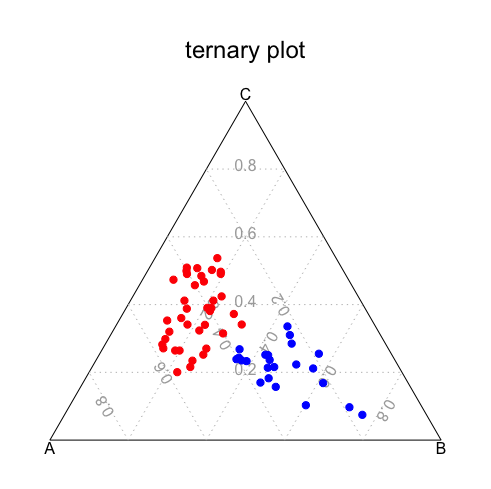
	A	B	C
$\bullet$	29.831%	48.605%	21.564%
$\bullet$	43.713%	18.572%	37.715%

Figure 1: $n=61$ points in $\mathcal{S}_{3}$, with a toy dataset.

If we define the binary operator $\diamond$ on $\mathcal{S}_{d}$,

$$\mathbf{x}\diamond\mathbf{y}=\left[{\frac{x_{1}y_{1}}{\sum_{i=1}^{d}x_{i}y_{i}}},\cdots,{\frac{x_{d}y_{d}}{\sum_{i=1}^{d}x_{i}y_{i}}}\right],$$

then $({\mathcal{S}_{d}},\diamond)$ is a commutative group, with identity element $d^{-1}\mathbf{1}$, and the inverse of $\mathbf{x}$ is

$$\mathbf{x}^{-1}=\left[{\frac{1/x_{1}}{\sum_{i=1}^{d}1/x_{i}}},\cdots,{\frac{1/x_{d}}{\sum_{i=1}^{d}1/x_{i}}}\right]=\mathcal{C}(1/\mathbf{x}).$$

5 Using an Alternative Representation of Simplex Data

A first strategy to define a transport mapping could be to use some isomorphism, $h:\mathcal{S}_{d}\rightarrow\mathcal{E}$ and then define the inverse mapping $h^{-1}:\mathcal{E}\rightarrow\mathcal{S}_{d}$, where $\mathcal{E}$ is some Euclidean space, classically $\mathbb{R}^{d-1}$, where the standard quadratic cost can be considered. This idea corresponds to the dual transport problem in Pal and Wong (2018).

5.1 Classical Transformations

The additive log ratio (alr) transform is an isomorphism where ${\displaystyle\operatorname{alr}:\mathcal{S}_{d}\rightarrow\mathbb{R}^{d-1}}$, given by

$${\displaystyle\operatorname{alr}(\mathbf{x})=\left[\log{\frac{x_{1}}{x_{d}}},\cdots,\log{\frac{x_{d-1}}{x_{d}}}\right]}.$$

Its inverse is, for any $\mathbf{z}\in\mathbb{R}^{d-1}$,

$${\displaystyle\operatorname{alr}^{-1}(\mathbf{z})=\mathcal{C}(\exp(z_{1}),\cdots,\exp(z_{d-1}),1)=\mathcal{C}\big{(}\exp([\mathbf{z},0])\big{)}}.$$

Such a map, from $\mathcal{S}_{d}$ to $\mathbb{R}^{d-1}$ is related to the so-called “exponential coordinate system” of the unit simplex, in Pal (2024). The center log ratio (clr) transform is both an isomorphism and an isometry where ${\displaystyle\operatorname{clr}:S^{d}\rightarrow\mathbb{R}^{d}}$,

$${\displaystyle\operatorname{clr}(\mathbf{x})=\left[\log{\frac{x_{1}}{\overline{\mathbf{x}}_{g}}},\cdots,\log{\frac{x_{D}}{\overline{\mathbf{x}}_{g}}}\right]},$$

where $\overline{\mathbf{x}}_{g}$ denotes the geometric mean of $\mathbf{x}$. Observe that the inverse of this function is the softmax function, i.e.,

$${\displaystyle\operatorname{clr}^{-1}(\mathbf{z})=\mathcal{C}(\exp(z_{1}),\cdots,\exp(z_{d}))=\mathcal{C}\big{(}\exp(\mathbf{z})\big{)}},\leavevmode\nobreak\ \mathbf{z}\in\mathbb{R}^{d}.$$

Finally, the isometric log ratio (ilr) transform, defined in Egozcue et al. (2003), is both an isomorphism and an isometry where ${\displaystyle\operatorname{ilr}:\mathcal{S}_{d}\rightarrow\mathbb{R}^{d-1}}$,

$${\displaystyle\operatorname{ilr}(\mathbf{x})={\big{[}}\langle\mathbf{x},\vec{e}_{1}\rangle,\cdots,\langle\mathbf{x},\vec{e}_{d-1}\rangle{\big{]}}}$$

for some orthonormal base $\{\vec{e}_{1},\cdots,\vec{e}_{d-1},\vec{e}_{d}\}$ of $\mathbb{R}^{d}$. One can consider some matrix $\mathbf{M}$, $d\times(d-1)$ such that $\mathbf{M}\mathbf{M}^{\top}=\mathbb{I}_{d-1}$ and $\mathbf{M}^{\top}\mathbf{M}=\mathbb{I}_{d}+\boldsymbol{1}_{d\times d}$. Then

$${\displaystyle\operatorname{ilr}(\mathbf{x})=\operatorname{clr}(\mathbf{x})\mathbf{M}=\log(\mathbf{x})\mathbf{M}},$$

and

$${\displaystyle\operatorname{ilr}^{-1}(\mathbf{z})=\mathcal{C}\big{(}(\exp(\mathbf{z}\mathbf{M}^{\top})\big{)}},\leavevmode\nobreak\ \mathbf{z}\in\mathbb{R}^{d-1}.$$

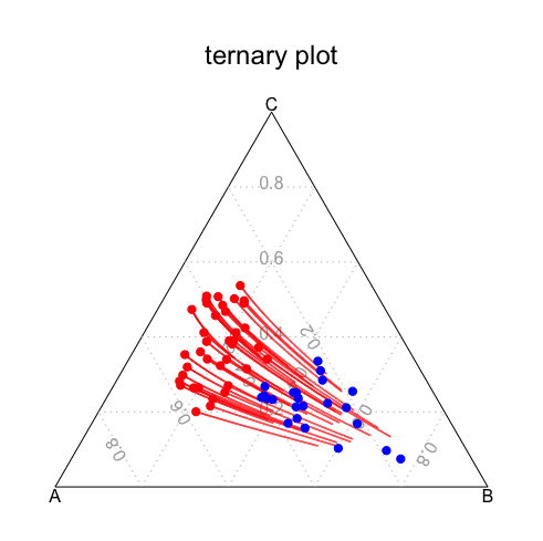
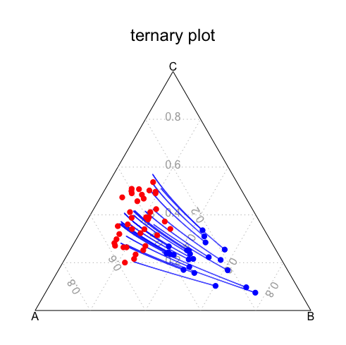
	A	B	C
$\bullet$ (0)	43.713%	18.572%	37.715%
$\bullet$ (1)	29.831%	48.605%	21.564%
$T($$\bullet$$)$	29.553%	48.517%	21.930%

	A	B	C
$\bullet$ (0)	43.713%	18.572%	37.715%
$\bullet$ (1)	29.831%	48.605%	21.564%
$T($$\bullet$$)$	43.728%	18.553%	37.719%

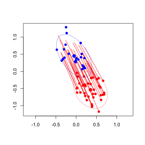
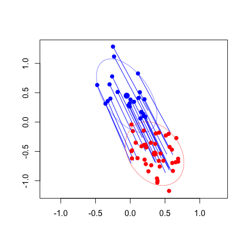
Figure 2: Counterfactuals using the $\operatorname{ilr}$ transformation, and Gaussian optimal transports, $\mu_{{\color[rgb]{1,0,0}0}}\mapsto\mu_{{\color[rgb]{0,0,1}1}}$ on the left, and $\mu_{{\color[rgb]{0,0,1}1}}\mapsto\mu_{{\color[rgb]{1,0,0}0}}$ on the right. Below are the averages of $\mathbf{x}_{{\color[rgb]{1,0,0}0},i}$’s and $\mathbf{x}_{{\color[rgb]{0,0,1}1},i}$’s, and of the transported points. The lines are geodesics in the dual spaces, mapped in the simplex. Optimal transport in $\mathbb{R}^{2}$, on $\mathbf{z}_{{\color[rgb]{1,0,0}0},i}$’s and $\mathbf{z}_{{\color[rgb]{0,0,1}1},i}$’s, can be visualized at the bottom (with linear mapping since Gaussian assumptions are made).

5.2 Gaussian Mapping in the Euclidean Representation

Given a random vector $\mathbf{X}$ in $\mathcal{S}_{d}$, we say that $\mathbf{x}$ follows a “normal distribution on the simplex” if, for some isomorphism $h$, the vector of orthonormal coordinates, $\mathbf{Z}=h(\mathbf{X})$ follows a multivariate normal distribution on $\mathbb{R}^{d-1}$. If we suppose that both $\mathbf{X}_{0}$ and $\mathbf{X}_{1}$, taking values in $\mathcal{S}_{d}$, follow “normal distributions on the simplex,” then we can use standard Gaussian optimal transport, between $\mathbf{Z}_{0}$ and $\mathbf{Z}_{1}$. For convenience, suppose that the same isomorphism is used for both distributions (but that assumption can easily be relaxed). Hence, if $\mathbf{Z}_{0}\sim\mathcal{N}(\boldsymbol{\mu}_{0},\boldsymbol{\Sigma}_{0})$ and $\mathbf{Z}_{1}\sim\mathcal{N}(\boldsymbol{\mu}_{1},\boldsymbol{\Sigma}_{1})$, the optimal mapping is linear,

$$\mathbf{z}_{1}=T^{\star}(\mathbf{z}_{0})=\boldsymbol{\mu}_{1}+\boldsymbol{A}(\mathbf{z}_{0}-\boldsymbol{\mu}_{0}),$$ (4)

where $\boldsymbol{A}$ is a symmetric positive matrix that satisfies $\boldsymbol{A}\boldsymbol{\Sigma}_{0}\boldsymbol{A}=\boldsymbol{\Sigma}_{1}$, which has a unique solution given by $\boldsymbol{A}=\boldsymbol{\Sigma}_{0}^{-1/2}\big{(}\boldsymbol{\Sigma}_{0}^{1/2}\boldsymbol{\Sigma}_{1}\boldsymbol{\Sigma}_{0}^{1/2}\big{)}^{1/2}\boldsymbol{\Sigma}_{0}^{-1/2}$, where $\boldsymbol{M}^{1/2}$ is the square root of the square (symmetric) positive matrix $\boldsymbol{M}$ based on the Schur decomposition ($\boldsymbol{M}^{1/2}$ is a positive symmetric matrix), as described in Higham (2008). Interestingly, it is possible to derive McCann’s displacement interpolation, from McCann (1997), to have some sort of continuous mapping $T_{t}^{\star}$ such that $T_{1}^{\star}=T^{\star}$ and $T_{0}=Id$, and so that $\mathbf{Z}_{t}=T_{t}^{\star}(\mathbf{Z}_{0})$ has distribution $\mathcal{N}(\boldsymbol{\mu}_{t},\boldsymbol{\Sigma}_{t})$ where $\boldsymbol{\mu}_{t}=(1-t)\boldsymbol{\mu}_{0}+t\boldsymbol{\mu}_{1}$ and

$$\boldsymbol{\Sigma}_{t}=\boldsymbol{\Sigma}_{0}^{-1/2}\left((1-t)\boldsymbol{\Sigma}_{0}+t\left(\boldsymbol{\Sigma}_{0}^{1/2}\boldsymbol{\Sigma}_{1}\boldsymbol{\Sigma}_{0}^{1/2}\right)^{1/2}\right)^{2}\boldsymbol{\Sigma}_{0}^{-1/2}.$$

Algorithm 2 Gaussian Based Transport of $\mathbf{x}_{0}$ on $\mathcal{S}_{d}$

Input: $\mathbf{x}_{0}$ ($\in\mathcal{S}_{d}$)
Parameter: $\{\mathbf{x}_{0,1},\cdots,\mathbf{x}_{0,n_{0}}\}$ and $\{\mathbf{x}_{1,1},\cdots,\mathbf{x}_{1,n_{1}}\}$ in $\mathcal{S}_{d}$;
Parameter: isomorphic transformation $h:\mathcal{S}_{d}\to\mathbb{R}^{d-1}$
Output: $\mathbf{x}_{1}$

 for $i\in\{1,\cdots,n_{0}\}$ do

   $\mathbf{z}_{0,i}\leftarrow h(\mathbf{x}_{0,i})$

 end for

 for $i\in\{1,\cdots,n_{1}\}$ do

   $\mathbf{z}_{1,i}\leftarrow h(\mathbf{x}_{1,i})$

 end for

 $\mathbf{m}_{0}\leftarrow$ average of $\{\mathbf{z}_{0,1},\cdots,\mathbf{z}_{0,n_{0}}\}$

 $\mathbf{m}_{1}\leftarrow$ average of $\{\mathbf{z}_{1,1},\cdots,\mathbf{z}_{1,n_{1}}\}$

 $\mathbf{S}_{0}\leftarrow$ empirical variance matrix of $\{\mathbf{z}_{0,1},\cdots,\mathbf{z}_{0,n_{0}}\}$

 $\mathbf{S}_{1}\leftarrow$ empirical variance matrix of $\{\mathbf{z}_{1,1},\cdots,\mathbf{z}_{1,n_{1}}\}$

 $\boldsymbol{A}\leftarrow\boldsymbol{S}_{0}^{-1/2}\big{(}\boldsymbol{S}_{0}^{1/2}\boldsymbol{S}_{1}\boldsymbol{S}_{0}^{1/2}\big{)}^{1/2}\boldsymbol{S}_{0}^{-1/2}$

 $\mathbf{x}_{1}\leftarrow\displaystyle{h^{-1}\big{(}\mathbf{m}_{1}+\boldsymbol{A}(h(\mathbf{x}_{0})-\mathbf{m}_{0})\big{)}}$

Empirically, this can be performed using Algorithm 2, and a simulation can be visualized in Figure 2, where $h=\operatorname{clr}$. On the left, we can visualize the mapping of red points to the blue distribution, and on the right, the “inverse mapping" of blue points to the red distribution. Transformed points $\mathbf{z}=h(\mathbf{x})$, that are plotted at the bottom, are supposed to be normally distributed, and a multivariate Gaussian Optimal Transport mapping is used. Hence, $T_{t}^{\star}$ is linear in $\mathbb{R}^{d-1}$, as given by expression 4, as well as displacement interpolation, corresponding to red and blue segments. But, as we can see on top of Figure 2, in the original space, $t\mapsto\mathbf{x}_{t}:=h^{-1}(\mathbf{z}_{t})$ will be nonlinear. Tables are average values of the three components of $\mathbf{x}$’s and $T^{\star}(\mathbf{x})$’s.

6 Optimal Transport for Measures on $\mathcal{S}_{d}$

6.1 Theoretical Properties

A function $\psi:\mathcal{S}_{d}\to\mathbb{R}$ is exponentially concave if $\exp[\psi]:\mathcal{S}_{d}\to\mathbb{R}_{+}$ is concave. As a consequence, such a function $\psi$ is differentiable almost everywhere. Let $\nabla\psi$ and $\nabla_{\vec{u}}\psi$ denote, respectively, its gradient, and its directional derivative. Following Pal and Wong (2016, 2018, 2020), define an allocation map generated by $\psi$, $\pi_{\psi}:\mathcal{S}_{d}\to\mathcal{S}_{d}$ defined as

$$\pi_{\psi}(\mathbf{x})=\left[x_{1}\big{(}1+\nabla_{\vec{e}_{1}-\mathbf{x}}\psi(\mathbf{x})\big{)},\cdots,x_{d}\big{(}1+\nabla_{\vec{e}_{d}-\mathbf{x}}\psi(\mathbf{x})\big{)}\right],$$

where $\{\vec{e}_{1},\cdots,\vec{e}_{d}\}$ is the standard orthonormal basis of $\mathbb{R}^{d}$. Consider the optimal transport problem with the following cost function, on $\mathcal{S}_{d}\times\mathcal{S}_{d}$, i.e., the L-divergence corresponding to the cross-entropy,

$$c(\mathbf{x},\mathbf{y})=\log\left(\frac{1}{d}\sum_{i=1}^{d}\frac{y_{i}}{x_{i}}\right)-\frac{1}{d}\sum_{i=1}^{d}\log\left(\frac{y_{i}}{x_{i}}\right),$$ (5)

called “Dirichlet transport” in Baxendale and Wong (2022). See Pistone and Shoaib (2024) for a discussion about the connections with the distance induced by Aitchsion’s inner product of Equation (3). From Theorem 1 in Pal and Wong (2020), for this cost function, there exists an exponentially concave function $\psi^{\star}:\mathcal{S}_{d}\to\mathbb{R}$ such that

$$T^{\star}(\mathbf{x})=\mathbf{x}\diamond\pi_{\psi^{\star}}\big{(}\mathbf{x}^{-1}\big{)}$$

defines a push-forward from $\mathbb{P}_{0}$ to $\mathbb{P}_{1}$, and the coupling $(\mathbf{x},T^{\star}(\mathbf{x}))$ is optimal for problem (1), and is unique if $\mathbb{P}_{0}$ is absolutely continuous. Observe that if $\mathbf{y}=T^{\star}(\mathbf{x})$,

$$\mathbf{y}=\mathcal{C}\big{(}\pi_{\psi^{\star}}\big{(}\mathbf{z}\big{)}_{1}/z_{1},\cdots,\pi_{\psi^{\star}}\big{(}\mathbf{z}\big{)}_{d}/z_{d}\big{)},$$

where $\mathbf{z}=\mathbf{x}^{-1}$.

One can also consider an interpolation,

$$T^{\star}_{t}(\mathbf{x})=\mathbf{x}\diamond\pi_{t}\big{(}\mathbf{x}^{-1}\big{)}$$

where $\pi_{t}=(1-t)d^{-1}\boldsymbol{1}+t\pi_{\psi^{\star}}$ (even if this approach differs from McCann’s displacement interpolation).

Note that a classical distribution on $\mathcal{S}_{d}$ is Dirichlet distribution, with density

$${\displaystyle f\left(x_{1},\ldots,x_{d};\boldsymbol{\alpha}\right)={\frac{1}{\mathrm{B}({\boldsymbol{\alpha}})}}\prod_{i=1}^{d}x_{i}^{\alpha_{i}-1}}$$

for some ${\boldsymbol{\alpha}}=(\alpha_{1},\ldots,\alpha_{d})\in\mathbb{R}_{+}^{d}$, and a normalizing constant denoted $\mathrm{B}({\boldsymbol{\alpha}})$. Level curves of the density of Dirichlet distributions fitted on our toy datasetcan be visualized in Figure 3. Unfortunately, unlike the multivariate Gaussian distribution, there is no explicit expression for the optimal mapping between Dirichlet distribution (regardless of the cost). Therefore, to remain within $\mathcal{S}_{d}$ and avoid the $\mathbb{R}^{d-1}$ representation, numerical techniques should be considered.

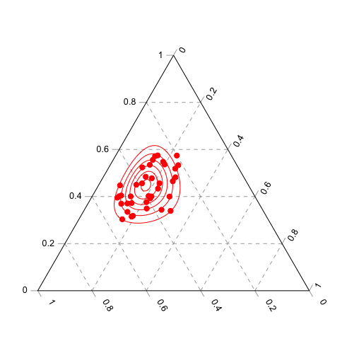
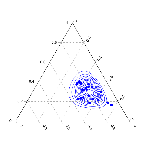
Figure 3: Densities of Dirchlet distributions in $\mathcal{S}_{3}$ fitted on observations of the toy dataset of Figure 1.

6.2 Matching

Consider two samples in the $\mathcal{S}_{d}$ simplex, $\{\mathbf{x}_{0,1},\cdots,\mathbf{x}_{0,n_{0}}\}$ and $\{\mathbf{x}_{1,1},\cdots,\mathbf{x}_{1,n_{1}}\}$. The discrete version of the Kantorovich problem (corresponding to Equation 2) is

$$\underset{\mathrm{P}\in U(n_{0},n_{1})}{\min}\left\{\sum_{i=1}^{{n_{0}}}\sum_{j=1}^{{n_{1}}}\mathrm{P}_{i,j}\mathrm{C}_{i,j}\right\}$$ (6)

where, as in Brualdi (2006), $U(n_{0},n_{1})$ is the set of ${n_{0}}\times{n_{1}}$ matrices corresponding to the convex transportation polytope

$$U(n_{0},n_{1})=\left\{\mathrm{P}:\mathrm{P}\boldsymbol{1}_{{n_{1}}}=\boldsymbol{1}_{n_{0}}\text{ and }{\mathrm{P}}^{\top}\boldsymbol{1}_{{n_{0}}}=\frac{n_{0}}{n_{1}}\boldsymbol{1}_{n_{1}}\right\},$$

and where $\mathrm{C}$ denotes the ${n_{0}}\times{n_{1}}$ cost matrix, $\mathrm{C}_{i,j}=c(\mathbf{x}_{i},\mathbf{x}_{j})$, associated with cost from Equation (5).

In Algorithm 3, we recall how this procedure works, which is the one explained in Peyré et al. (2019), with a specific cost function (from Equation (5)). In the toy dataset, this can be visualized for two specific observations $\mathbf{x}_{0,i}$. If $n_{0}\neq n_{1}$, it is not a one-to-one coupling, and “the counterfactual” is actually a weighted average of $\mathbf{x}_{1,j}$’s, where weights are given in row $\mathbf{P}^{\star}_{i}=[\mathbf{P}^{\star}_{i,1},\cdots,\mathbf{P}^{\star}_{i,n_{1}}]\in\mathcal{S}_{n_{1}}$.

Algorithm 3 Coupling samples on $\mathcal{S}_{d}$

Input: $\{\mathbf{x}_{0,1},\cdots,\mathbf{x}_{0,n_{0}}\}$ and $\{\mathbf{x}_{1,1},\cdots,\mathbf{x}_{1,n_{1}}\}$ in $\mathcal{S}_{d}$;
Output: weight matching matrix $n_{0}\times n_{1}$ $\mathbf{P}^{*}$

 $\mathbf{C}\leftarrow$ matrix $n_{0}\times n_{1}$, $\mathbf{C}_{i,j}=c(\mathbf{x}_{i},\mathbf{x}_{j})$ using (5)

 $\mathbf{P}^{\star}\leftarrow$ solution of Equation (6), using LP libraries

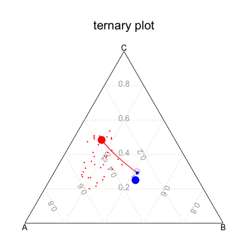
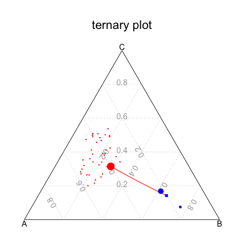
Figure 4: Getting empirical counterfactuals using matching techniques, with $\mathbf{x}_{{\color[rgb]{1,0,0}0},i}$ in red (on the top-left hand-side), and counterfactuals $\mathbf{x}_{{\color[rgb]{0,0,1}1},j}$’s in blue (bottom-right hand-side), with size proportional to $\mathbf{P}^{\star}_{i}=[\mathbf{P}^{\star}_{i,1},\cdots,\mathbf{P}^{\star}_{i,n_{1}}]\in\mathcal{S}_{n_{1}}$.

7 Application on Sequential Transport for Counterfactuals

Variables $\mathbf{x}_{j}$ in tabular data are either continuous or categorical. If $\mathbf{x}_{j}$ is continuous, since $\mathbf{x}_{j}\in\mathbb{R}$, transporting from observed $\mathbf{x}_{j}|s=0$ to counterfactual $\mathbf{x}_{j}|s=1$ is performed using standard (conditional) monotonic mapping, as discussed in Fernandes Machado et al. (2025), using classical $F_{1}^{-1}\circ F_{0}$. If $\mathbf{x}_{j}$ is categorical, with $d$ categories, consider some fitted model $\widehat{m}(\mathbf{x}_{j}|\mathbf{x}_{-j})$, using some multinomial loss, and let $\widehat{\mathbf{x}}_{j}=\widehat{m}(\mathbf{x}_{j}|\mathbf{x}_{-j})$ denote the predicted scores, so that $\widehat{\mathbf{x}}_{j}\in\mathcal{S}_{d}$. Then use Algorithm 2, with a Gaussian mapping in an Euclidean representation space, to transport from observed $\widehat{\mathbf{x}}_{j}|s=0$ to counterfactual $\widehat{\mathbf{x}}_{j}|s=1$, in $\mathcal{S}_{d}$.

7.1 German Credit: Purpose

In the popular German Credit dataset, from Hofmann (1994), the variable Purpose described the reason an individual took out a loan. This variable is an important predictor for explaining potential defaults. The original variable is based on ten categories, that are merged here into three main classes, cars, equipment and other, in order to visualize the transport in a ternary plot — or Gibbs triangle. The sensitive variable $s$ is here Sex.

We aim to construct a counterfactual value for the loan purpose, assuming the individuals were of a different sex. To achieve this, we apply our suggested procedure from to represent the purpose categorical variable as a compositional variable, using the same four models outlined in Section 3 and then apply Gaussian mapping from Section 5.2. The results provided by all of the models, shown in Figure 5, suggest that, had the individuals been of a different sex, the purpose of the loan would have changed. Specifically, if the average scores in each group (cars, equipment, and other) were approximately $[35\%,45\%,20\%]$ in the female population, after transporting to obtain the counterfactuals, the average scores become $[31\%,52\%,18\%]$, which closely resemble the actual frequencies of each category in the original male population.

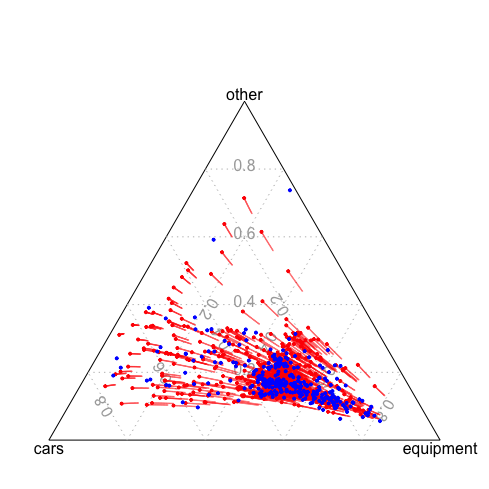
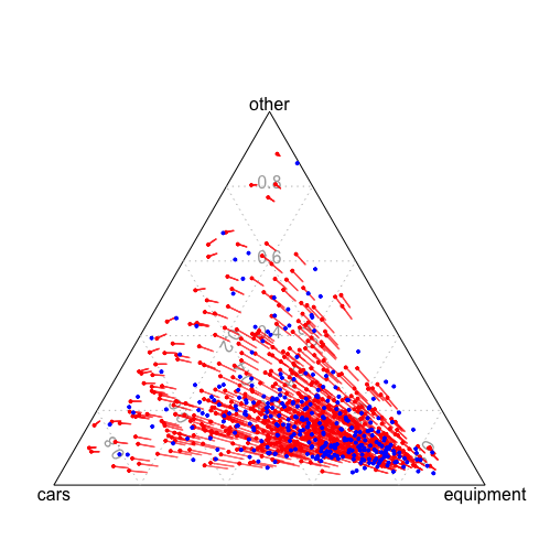
categorical $\bullet$ (M)

categorical $\bullet$ (F)

[1pt/1pt] composition $\bullet$ (M)

composition $\bullet$ (F)

$T($$\bullet$$)$

MLR (1)
cars	equipmt.	other
30.323%	53.226%	16.452%
35.217%	44.638%	20.145%
[1pt/1pt] 31.106%	51.328%	17.565%
34.865%	45.490%	19.645%
31.016%	51.418%	17.566%

MLR (2)
cars	equipmt.	other
30.323%	53.226%	16.452%
35.217%	44.638%	20.145%
[1pt/1pt] 31.955%	50.539%	17.507%
34.484%	45.845%	19.671%
31.855%	50.570%	17.575%

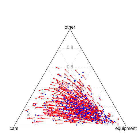
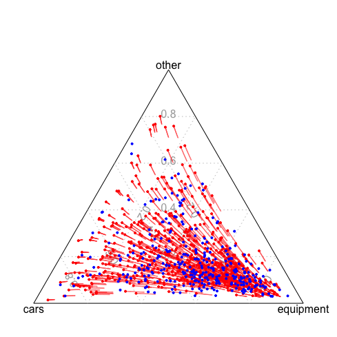
composition $\bullet$ (M)

composition $\bullet$ (F)

$T($$\bullet$$)$

random forest
cars	equipmt.	other
32.055%	49.882%	18.063%
34.977%	45.409%	19.614%
32.046%	49.883%	18.070%

boosting
cars	equipmt.	other
31.843%	50.712%	17.445%
34.714%	45.341%	19.945%
31.871%	50.675%	17.455%

Figure 5: Optimal transport using the $\operatorname{clr}$ transformation, and Gaussian optimal transports, on the purpose scores in the German Credit database, with two logistic GAM models to predict scores, on top, and below a random forest (left) and a boosting model (right). Points in red are compositions for women, while points in blue are for men. Lines indicate the displacement interpolation when generating counterfactuals.

One can also consider our second approach, using matching in $\mathcal{S}_{3}$. Consider individual $i$ among women, e.g., the left of Figure 6, $x_{0,i}=$ “equipment.” Using a MLR model, we obtain composition $\mathbf{x}_{0,i}$, here $[11.38\%,79.30\%,9.32]$. Using Algorithm 3, three points $\mathbf{x}_{1,j}$’s are matched, respectively with weights $[0.453,0.094,0.453]$. The first and the third individuals are such that $x_{1,j}=$ “equipment” too, the second one “other.” So it would make sense to suppose that the counterfactual version of woman $i$ with an “equipment” credit is a man with the same purpose. Actually, using Gaussian transport, $T^{\star}(\mathbf{x}_{0,i})=[15.78\%,69.54\%,14.68\%]$.

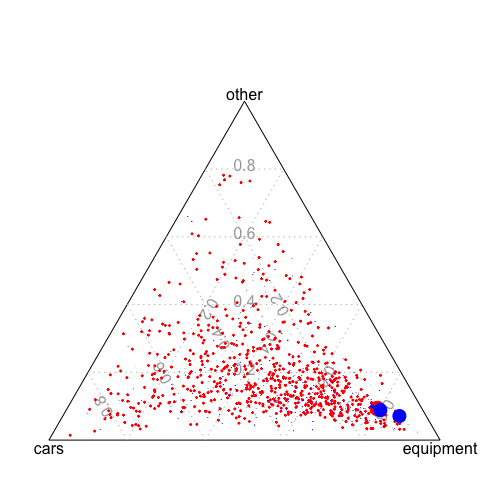
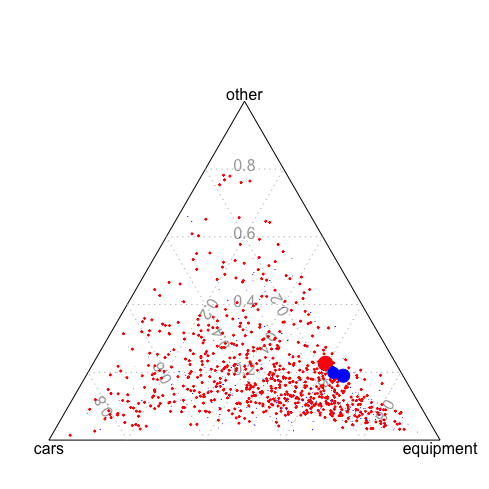
Figure 6: Empirical matching of two women, in red, from the German Credit dataset, with 2 or 3 men, in blue. Size of blue dots are proportional to the weights $\mathbf{P}^{\star}_{i}$.

7.2 Adult: Marital Status

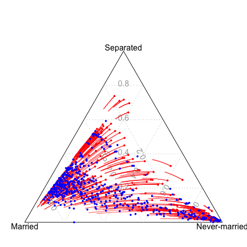
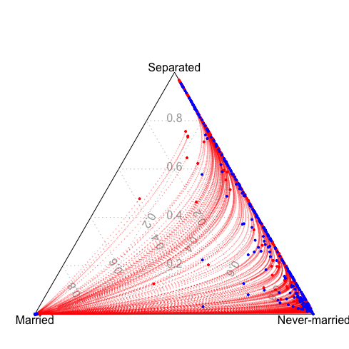
categorical $\bullet$ (M)

categorical $\bullet$ (F)

[1pt/1pt] composition $\bullet$ (M)

composition $\bullet$ (F)

$T($$\bullet$$)$

GAM-MLR (1)
Mar.	Never M	Sep.
61.752%	26.609%	11.639%
15.130%	44.204%	40.667%
[1pt/1pt] 51.441%	29.641%	18.918%
35.180%	39.714%	25.106%
49.857%	30.740%	19.403%

GAM-MLR (2)
Mar.	Never M	Sep.
61.752%	26.609%	11.639%
15.130%	44.204%	40.667%
[1pt/1pt] 59.819%	27.276%	12.905%
12.982%	46.093%	40.925%
67.214%	24.678%	8.108%

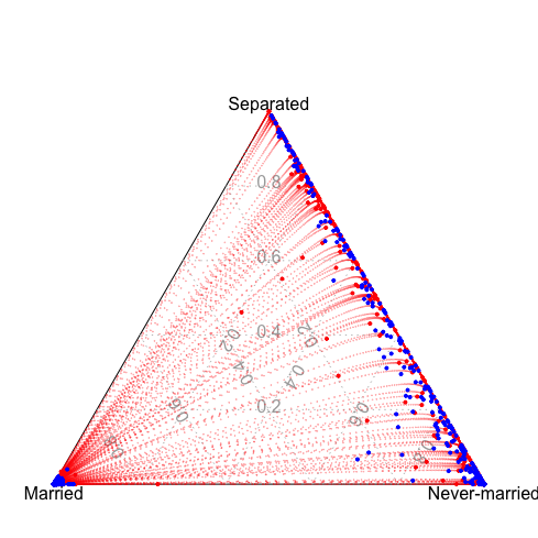
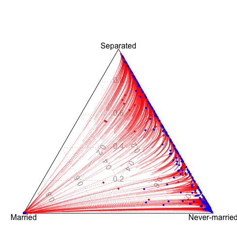
composition $\bullet$ (M)

composition $\bullet$ (F)

$T($$\bullet$$)$

random forest
Mar.	Never M	Sep.
59.619%	27.827%	12.554%
12.765%	48.707%	38.528%
46.306%	34.967%	18.727%

boosting
Mar.	Never M	Sep.
59.764%	27.250%	12.987%
13.219%	45.976%	40.805%
47.611%	30.313%	22.076%

Figure 7: Optimal transport using the $\operatorname{clr}$ transformation, and Gaussian optimal transports, on the Marital Status scores in the Adult database, with two logistic GAM-MLR models to predict scores, on top, and below a random forest (left) and a boosting model (right). Points in red are compositions for women, while points in blue are for men. Lines indicate the displacement interpolation when generating counterfactuals.

Following the numerical applications in Plečko et al. (2024) and Fernandes Machado et al. (2025), we consider here the Adult dataset, from Becker and Kohavi (1996). We regrouped categories of the Marital Status variable to create three generic ones (that can be visualized in a ternary plot, as in Figure 7), namely Married, Never-married and Separated. This example is interesting because if we compare status with respect to the Sex variable, proportions are quite different. In the dataset, proportions for married, never married, and separated are (roughly) $[62\%,27\%,12\%]$ for men, $[14\%,44\%,41\%]$ for women (more precise values are at the top of the table in Figure 7). Thus, the counterfactual of a “separated” woman is more likely to be a “married” man than a “separated” man. Four models are used to convert the categorical variable Marital Status into a composition, as previously. The first MLR is based on three variables: a categorical variable, occupation, and two continuous ones, age, and hours_per_week, modeled nonlinearly using $b$-splines (hence, it is referred to as a logistic GAM). This model is clearly underfitted. Therefore, observations $\mathbf{x}_{{\color[rgb]{1,0,0}0},i}$’s for women and $\mathbf{x}_{{\color[rgb]{0,0,1}1},i}$’s for men clearly are in the interior of $\mathcal{S}_{d}$. In contrast, the more complex MLR (which uses additional features), as well as the random forest and boosting models, can produce predictions near the simplex boundary, $\partial\mathcal{S}_{d}$.

For the underfitted model (top left), transported scores have a distribution very close to the ones in the population of men. For the more accurate MLR model (top right), proportions are very close to the actual proportions (which is not surprising since GLMs are usually well calibrated), but the transported scores are slightly different than the proportions of categories (proportions were $[62\%,27\%,12\%]$ while average transported scores are $[67\%,25\%,8\%]$). At least, we are different from the original ones, but the mapping is not as accurate as it should be. This might come from the fact that when the points $\mathbf{x}_{i}$ are close to the border $\partial\mathcal{S}_{d}$, it is quite unlikely that the sample $\mathbf{z}_{i}$ is Gaussian.

8 Conclusion

In this article, we introduce a novel approach for constructing counterfactuals for categorical data by transforming them into compositional data using a probabilistic classifier. Our approach avoids imposing arbitrary assumptions about label ordering. However, our methodology is not without limitations. Optimal transport computations, particularly on the simplex, can be computationally intensive for large-scale datasets, posing challenges in high-dimensional settings. Additionally, the reliance on a probabilistic classifier in the initial step introduces potential vulnerabilities. Biases may arise if the classifier is poorly calibrated or inaccurate, which would affect the quality of the subsequent analysis.

References

- Aitchison (1982) Aitchison, J. (1982). The statistical analysis of compositional data. Journal of the Royal Statistical Society: Series B (Methodological) 44: 139–160.
- Baxendale and Wong (2022) Baxendale, P. and Wong, T.-K. L. (2022). Random concave functions. The Annals of Applied Probability 32: 812–852.
- Becker and Kohavi (1996) Becker, B. and Kohavi, R. (1996). Adult. UCI Machine Learning Repository, doi:10.24432/C5XW20.
- Black et al. (2020) Black, E., Yeom, S. and Fredrikson, M. (2020). Fliptest: fairness testing via optimal transport. In Proceedings of the 2020 Conference on Fairness, Accountability, and Transparency, 111–121.
- Brenier (1991) Brenier, Y. (1991). Polar factorization and monotone rearrangement of vector-valued functions. Communications on pure and applied mathematics 44: 375–417, doi:10.1002/cpa.3160440402.
- Brualdi (2006) Brualdi, R. A. (2006). Combinatorial matrix classes, 13. Cambridge University Press.
- Charpentier et al. (2023) Charpentier, A., Flachaire, E. and Gallic, E. (2023). Optimal transport for counterfactual estimation: A method for causal inference. In Optimal Transport Statistics for Economics and Related Topics. Springer, 45–89.
- Chayes (1971) Chayes, F. (1971). Ratio correlation. University of Chicago Press.
- Cheng et al. (2010) Cheng, W., Hüllermeier, E. and Dembczynski, K. J. (2010). Bayes optimal multilabel classification via probabilistic classifier chains. In Proceedings of the 27th international conference on machine learning (ICML-10), 279–286.
- De Lara et al. (2024) De Lara, L., González-Sanz, A., Asher, N., Risser, L. and Loubes, J.-M. (2024). Transport-based counterfactual models. Journal of Machine Learning Research 25: 1–59.
- Egozcue et al. (2003) Egozcue, J. J., Pawlowsky-Glahn, V., Mateu-Figueras, G. and Barcelo-Vidal, C. (2003). Isometric logratio transformations for compositional data analysis. Mathematical geology 35: 279–300.
- Fernandes Machado et al. (2025) Fernandes Machado, A., Charpentier, A. and Gallic, E. (2025). Sequential Conditional Transport on Probabilistic Graphs for Interpretable Counterfactual Fairness. In Proceedings of the AAAI conference on artificial intelligence, 39.
- Hallin et al. (2021) Hallin, M., Del Barrio, E., Cuesta-Albertos, J. and Matrán, C. (2021). Distribution and quantile functions, ranks and signs in dimension d: A measure transportation approach. The Annals of Statistics 49: 1139–1165.
- Hallin and Konen (2024) Hallin, M. and Konen, D. (2024). Multivariate quantiles: Geometric and measure-transportation-based contours. In Applications of Optimal Transport to Economics and Related Topics. Springer, 61–78.
- Higham (2008) Higham, N. J. (2008). Functions of matrices: theory and computation. SIAM.
- Hofmann (1994) Hofmann, H. (1994). German Credit Data. UCI Machine Learning Repository, doi:10.24432/C5NC77.
- Imai et al. (2022) Imai, K., Olivella, S. and Rosenman, E. T. (2022). Addressing census data problems in race imputation via fully bayesian improved surname geocoding and name supplements. Science Advances 8: eadc9824, doi:10.1126/sciadv.adc9824.
- Kantorovich (1942) Kantorovich, L. V. (1942). On the translocation of masses. In Doklady Akademii Nauk USSR, 37, 199–201.
- King et al. (2004) King, G., Tanner, M. A. and Rosen, O. (2004). Ecological inference: New methodological strategies. Cambridge University Press.
- Kusner et al. (2017) Kusner, M. J., Loftus, J., Russell, C. and Silva, R. (2017). Counterfactual fairness. In Guyon, I., Luxburg, U. V., Bengio, S., Wallach, H., Fergus, R., Vishwanathan, S. and Garnett, R. (eds), Advances in Neural Information Processing Systems 30. NIPS, 4066–4076.
- McCann (1997) McCann, R. J. (1997). A convexity principle for interacting gases. Advances in mathematics 128: 153–179.
- Monge (1781) Monge, G. (1781). Mémoire sur la théorie des déblais et des remblais. Histoire de l’Académie Royale des Sciences de Paris .
- Naeini et al. (2015) Naeini, M. P., Cooper, G. and Hauskrecht, M. (2015). Obtaining well calibrated probabilities using bayesian binning. In Proceedings of the AAAI conference on artificial intelligence, 29.
- Pal (2024) Pal, S. (2024). On the difference between entropic cost and the optimal transport cost. The Annals of Applied Probability 34: 1003–1028.
- Pal and Wong (2016) Pal, S. and Wong, T.-K. L. (2016). The geometry of relative arbitrage. Mathematics and Financial Economics 10: 263–293.
- Pal and Wong (2018) Pal, S. and Wong, T.-K. L. (2018). Exponentially concave functions and a new information geometry. The Annals of probability 46: 1070–1113.
- Pal and Wong (2020) Pal, S. and Wong, T.-K. L. (2020). Multiplicative schrödinger problem and the dirichlet transport. Probability Theory and Related Fields 178: 613–654.
- Pawlowsky-Glahn and Egozcue (2001) Pawlowsky-Glahn, V. and Egozcue, J. J. (2001). Geometric approach to statistical analysis on the simplex. Stochastic Environmental Research and Risk Assessment 15: 384–398.
- Peyré et al. (2019) Peyré, G., Cuturi, M. et al. (2019). Computational optimal transport: With applications to data science. Foundations and Trends in Machine Learning 11: 355–607.
- Pistone and Shoaib (2024) Pistone, G. and Shoaib, M. (2024). A unified approach to aitchison’s, dually affine, and transport geometries of the probability simplex. Axioms : 823.
- Plečko and Meinshausen (2020) Plečko, D. and Meinshausen, N. (2020). Fair data adaptation with quantile preservation. Journal of Machine Learning Research 21: 1–44.
- Plečko et al. (2024) Plečko, D., Bennett, N. and Meinshausen, N. (2024). Fairadapt: Causal reasoning for fair data preprocessing. Journal of Statistical Software 110: 1–35.
- Santambrogio (2015) Santambrogio, F. (2015). Optimal transport for applied mathematicians. Springer.
- Villani (2003) Villani, C. (2003). Topics in optimal transportation, 58. American Mathematical Society.
- Zadrozny and Elkan (2001) Zadrozny, B. and Elkan, C. (2001). Obtaining calibrated probability estimates from decision trees and naive Bayesian classifiers. In Proceedings of the Eighteenth International Conference on Machine Learning, ICML ’01. San Francisco, CA, USA: Morgan Kaufmann Publishers Inc., 609–616.