Partial Smoothness, Subdifferentials and Set-valued Operators

Abstract

Over the past decades, the concept “partial smoothness” has been playing as a powerful tool in several fields involving nonsmooth analysis, such as nonsmooth optimization, inverse problems and operation research, etc. The essence of partial smoothness is that it builds an elegant connection between the optimization variable and the objective function value through the subdifferential. Identifiability is the most appealing property of partial smoothness, as locally it allows us to conduct much finer or even sharp analysis, such as linear convergence or sensitivity analysis. However, currently the identifiability relies on non-degeneracy condition and exact dual convergence, which limits the potential application of partial smoothness. In this paper, we provide an alternative characterization of partial smoothness through only subdifferentials. This new perspective enables us to establish stronger identification results, explain identification under degeneracy and non-vanishing error. Moreover, we can generalize this new characterization to set-valued operators, and provide a complement definition of partly smooth operator proposed in [14].

Key words. Nonsmooth optimization, Partial Smoothness, Subdifferential, Set-valued Operators

AMS subject classifications. 47H05, 90C31, 49M05, 65K10,

1 Introduction

Nonsmoothness is at the heart of modern optimization, the advances in nonsmooth analysis have greatly impacted the development of (first-order) optimization algorithms, and spread to many other fields including operation research, inverse problems, signal/image processing, data science and statistics, to name a few. Along the study of nonsmoothness, an important topic is exploring the underlying smooth structure, especially around the optimal solutions. Such results not only yield high-level geometrical understanding of the optimization problem, but also stimulate the development of efficient numerical schemes. This direction of research dates back to linear programming where complementary slackness captures the smoothness inside constraints which is the principle of active set methods. Wright extends this idea to smooth identifiable surfaces [34], which is further extended to smooth Riemannian manifold by Lewis and Hare [10] and encoded as “partial smoothness”. Another similar branch of work is called “$\mathcal{U}\mathcal{V}$ decomposition” [11], see also [25].

An important property of the smooth structure is called “identifiability”. This means that given an optimization problem $\min_{x}f(x)$ whose optimal solution(s) are contained in a smooth Riemannian manifold $\mathcal{M}$, a sequence, e.g. $\{x^{(k)}\}_{k\in\mathbb{N}}$, is generated to find an optimal solution $x^{\star}\in\mathcal{M}$, then for all $k$ large enough, there holds

$$x^{(k)}\in\mathcal{M}.$$ (1.1)

Under partial smoothness [12], identification (1.1) can be guaranteed if $x^{\star}$ is non-degenerate (i.e. $\bar{u}\in\mathrm{ri}\big{(}{\partial f(x^{\star})}\big{)}$ where $\mathrm{ri}\big{(}{\cdot}\big{)}$ denotes relative interior), and there exists dual sequence $\{u^{(k)}\}_{k\in\mathbb{N}}$ associated to $\{x^{(k)}\}_{k\in\mathbb{N}}$ satisfying

$$\partial f(x^{(k)})\ni u^{(k)}\to\bar{u}.$$ (1.2)

Since first proposed in [12], the theoretical framework of partial smoothness is established over a series of work [10, 13, 6], and finds successful applications in several fields including sensitivity analysis [26], local linear convergence analysis of first-order optimization algorithms [15, 20] and design efficient numerical schemes [28], etc.

Though very powerful, partial smoothness has several limitations, such as requiring non-degeneracy condition for identification, dual vector convergence and restricted to functions. Attempts are made in the literature to overcome them, for example in [9], for functions with stratifiable structure, the authors study the identification under degeneracy conditions. In [6], partial smoothness in terms of normal cone operator is studied. Later on in [14], partly smooth operator is proposed together with a so-called “constant rank” property which characterizes the local property of the operator’s graph. Unfortunately, these work fail to provide satisfactory solutions to the limitations of partial smoothness.

Contribution

Motivated by the limitations of partial smoothness, in this paper we propose a novel alternative definition (see Definition 3.4) of partial smoothness from functions to set-valued operators. Under this new definition, we are able to provide a finer local geometric characterization of non-degeneracy condition. From this, we have the following contributions

1. In Definition 3.4, we propose a new definition of partial smoothness of set-valued operator, which is a complement of the constant-rank property of [14], calculus rules are also provided.

2. We provide a new geometric characterization for partial smoothness. Take subdifferential $\partial f$ of partly smooth function $f$ for example, in Proposition 4.1, we show that the linear span of the local union $\mathcal{U}=\cup_{\{x\in\mathcal{M},{|\kern-1.125pt|}x-\bar{x}{|\kern-1.125pt|}<\varepsilon\}}(x+\partial f(x))$ is the whole space; Moreover, there holds $\bar{x}+\bar{u}\in\mathrm{int}(\mathcal{U})$, which directly leads to the identifiability of the manifold; see Proposition 4.1 and Theorem 4.3.

3. Owing to the new local characterization, we are able to show that identification still happens even if condition (1.2) fails, given that essentially $u^{(k)}$ is close enough to $\bar{u}$; see Theorem 4.3. In Corollary 4.13, we also discuss the identifiability without non-degenerate condition.

4. Under proper condition, identification only occurs for large enough $k$. In Proposition 4.15, we provide an smallest possible estimation of $k$ after which identification happens.

To illustrate these theoretical results, we apply our findings to variational inequalities and mini-batch stochastic gradient descent, demonstrating how our approach can effectively explain practical problems.

Paper organization

The following of the paper is organized as: in Section 2 we collect some necessary preliminarily materials. Section 3 introduces the concept of partial smoothness and outlines the fundamental properties of partial smooth operators. In Section 4, we discuss our main results regarding the identifiability of partly smooth operators, offering a new perspective on partial smoothness and extending identifiable conditions to more general cases. Finally, in Section 5, we provide several applications to illustrate the identification of partly smooth operators with concrete experimental results.

2 Notations and preliminaries

We denote $\mathbb{N}$ the set of non-negative integers and $k\in\mathbb{N}$ the index. $\bar{\mathbb{R}}=\mathbb{R}\cup\big{\{}+\infty\big{\}}$ denotes the extended real line. $\mathbb{R}^{n},\mathbb{R}^{m}$ are the standard finite dimensional Euclidean spaces, equipped with inner product $\langle\cdot,\,\cdot\rangle$ and norm ${|\kern-1.125pt|}\cdot{|\kern-1.125pt|}$.

Define ${\mathds{B}}_{r}(x)$ the ball with center $x$ and radius $r$. Let $\mathcal{S}\subset\mathbb{R}^{n}$ be a nonempty closed convex set, if its interior exists, we denote it as $\mathrm{int}(\mathcal{S})$, the boundary is denoted as $\mathrm{bdy}(\mathcal{S})$; If the interior does not exist, then $\mathrm{ri}(\mathcal{S})$ denotes its relative interior, and $\mathrm{rbd}(\mathcal{S})$ denotes the relative boundary. We denote $\mathrm{aff}(\mathcal{S})$ its affine hull, $\mathrm{par}(\mathcal{S})=\mathrm{aff}(\mathcal{S})-x,\forall x\in\mathcal{S}$ the subspace parallel to it. The distance function between a point $z\in\mathbb{R}^{n}$ and $\mathcal{S}$ is defined by

$$\mathrm{dist}(z,\mathcal{S})\stackrel{{\scriptstyle\text{\rm\tiny def}}}{{=}}\inf_{x\in\mathcal{S}}{|\kern-1.125pt|}z-x{|\kern-1.125pt|}.$$

Denote $\mathrm{\mathscr{P}}_{\mathcal{S}}$ the orthogonal projector onto $\mathcal{S}$ and ${\mathscr{N}}_{\mathcal{S}}$ its normal cone operator.

Given a proper, lower semi-continuous (l.s.c.) function $f:\mathbb{R}^{n}\to\bar{\mathbb{R}}$ and $x\in\mathrm{dom}(f)$, the Fréchet (or regular) subdifferential $\partial^{F}f(x)$ of $f$ at $x$, is the set of vectors $v\in\mathbb{R}^{n}$ that satisfies

$$\liminf_{z\to x,\,z\neq x}\,{{\frac{\raisebox{0.41669pt}{\footnotesize$1$}}{\raisebox{-1.24994pt}{\footnotesize${|\kern-1.125pt|}x-z{|\kern-1.125pt|}$}}}}(f(z)-f(x)-\langle v,\,z-x\rangle)\geq 0.$$

If $x\notin\mathrm{dom}(f)$, then $\partial^{F}f(x)=\emptyset$. The limiting-subdifferential (or simply subdifferential) of $f$ at $x$, written as $\partial f(x)$, is defined as

$$\partial f(x)\stackrel{{\scriptstyle\text{\rm\tiny def}}}{{=}}\Big{\{}v\in\mathbb{R}^{n}:\exists x^{(k)}\to x,f(x^{(k)})\to f(x),\,v^{(k)}\in\partial^{F}f(x^{(k)})\to v\Big{\}}.$$

Denote $\mathrm{dom}(\partial f)\stackrel{{\scriptstyle\text{\rm\tiny def}}}{{=}}\big{\{}x\in\mathbb{R}^{n}:\partial f(x)\neq\emptyset\big{\}}$, an element in $\partial f$ is called the subgradient.

Let $S\subseteq\mathbb{R}^{n}$ be a set, though indicator function $\iota_{S}(x)$ of the set, the Fréchet (or regular) normal cone to $S$ at a point $x\in S$ is defined by $\mathscr{N}^{F}_{S}(\bar{x})=\partial^{F}\iota_{S}(\bar{x})$, and the (limiting) normal cone is $\mathscr{N}_{S}(\bar{x})=\partial\iota_{S}(\bar{x})$. Both normal cones are defined to be empty for $x\notin S$. $S$ is said to be (Clarke) regular at $\bar{x}$ if it is locally closed at $\bar{x}$ and the two normal cones agree. Given a function $f:\mathbb{R}^{n}\to\bar{\mathbb{R}}$, its epi-graph is defined as ${\rm epi}(f)\stackrel{{\scriptstyle\text{\rm\tiny def}}}{{=}}\big{\{}(x,t)\in\mathbb{R}^{n}\times\mathbb{R}\mid f(x)\leq t\big{\}}$, then $f$ is regular at $\bar{x}$ if its epi-graph is regular at $(\bar{x},f(\bar{x}))$; in this case $\partial^{F}f(\bar{x})=\partial f(\bar{x})$.

2.1 Set-valued operators and motononicity

Let $A:\mathbb{R}^{n}\rightrightarrows\mathbb{R}^{n}$ be a set-valued operator, the domain of $A$ is $\mathrm{dom}(A)=\{x\in\mathbb{R}^{n}\mid A(x)\neq\emptyset\}$, the range of $A$ is $\mathrm{ran}(A)=\{u\in\mathbb{R}^{n}\mid\exists x\in\mathbb{R}^{n}:u\in A(x)\}$, the graph of $A$ is the set $\mathrm{gph}\,(A)=\{(x,u)\in\mathbb{R}^{n}\times\mathbb{R}^{n}\mid u\in A(x)\}$, and its zeros set is $\mathrm{zer}(A)=\{x\in\mathbb{R}^{n}\mid 0\in A(x)\}$. For any $u\in A(x)$, we call it a dual vector of $x$.

2.1.1 Continuity of set-valued operators

Different from single-valued analysis, there are two distinct concepts for the continuity of set-valued operators: lower semi-continuity and upper semi-continuity. The definitions below are from [1].

Definition 2.1 (Lower semi-continuity).

A set-valued operator $A:\mathbb{R}^{n}\rightrightarrows\mathbb{R}^{n}$ is called lower semi-continuous at $\bar{x}\in\mathrm{dom}(A)$ if and only if for any $\bar{u}\in A(\bar{x})$ and any sequence $x^{(k)}\in\mathrm{dom}(A)$ converging to $\bar{x}$, there exists a sequence of dual vectors $u^{(k)}\in A(x^{(k)})$ converging to $\bar{u}$. It is moreover said to be lower semi-continuous if it is lower semi-continuous at every point in $x\in\mathrm{dom}(A)$.

In the single-valued case, the above definition is equivalent to: for any open subset $\mathcal{U}\subset\mathbb{R}^{n}$ such that $\mathcal{U}\cap A(\bar{x})\neq\emptyset$,

$$\exists\eta>0\,\,\,\mathrm{s.t.}\,\,\,\forall x\in{\mathds{B}}_{\eta}(\bar{x}),\,A(x)\cap\mathcal{U}\neq\emptyset.$$

Definition 2.2 (Upper semi-continuity).

A set-valued operator $A:\mathbb{R}^{n}\rightrightarrows\mathbb{R}^{m}$ is called upper semi-continuous at $\bar{x}\in\mathrm{dom}(A)$ if and only if for any for any neighborhood $\mathcal{U}$ of $A(\bar{x})$,

$$\exists\eta>0\,\,\,\mathrm{s.t.}\,\,\,\forall x\in{\mathds{B}}_{\eta}(\bar{x}),\,A(x)\subset\mathcal{U}.$$

It is moreover said to be upper semi-continuous if it is upper semi-continuous at every point in $x\in\mathrm{dom}(A)$.

Alternatively, upper semi-continuity means that given a sequence $x^{(k)}\to\bar{x}$ with $u^{(k)}\in A(x^{(k)})$ and $u^{(k)}\to\bar{u}$, then there holds $\bar{u}\in A(\bar{x})$. When $A(x)$ is compact, $A$ is upper semi-continuous at $x$ if and only if

$$\forall\varepsilon>0,\,\exists\eta>0\,\,\,\mathrm{s.t.}\,\,\,\forall x\in{\mathds{B}}_{\eta}(\bar{x}),\,\,A(x)\subset{\mathds{B}}_{\varepsilon}(A(\bar{x})).$$

Noted that this definition is a natural extension of the definition of a continuous single-valued operator.

Lemma 2.3 ([31, Theorem 8.6, Proposition 8.7]).

Let $f:\mathbb{R}^{n}\to\bar{\mathbb{R}}$, and $x\in\mathrm{dom}(f)$ with $f(x)$ finite, then both $\partial^{F}f(x),\partial f(x$) are closed, with $\partial^{F}f(x)$ being convex and $\partial^{F}f(x)\subset\partial f(x)$. If $f$ is proper and lower semi-continuous functions, then its (limiting) subdifferential is upper semi-continuous.

2.1.2 Monotoncity of set-valued operators

Below we provide some basic definition of monotonicity, and refer to [3] for dedicated discussions.

Definition 2.4.

A set-valued operator $A:\mathbb{R}^{n}\rightrightarrows\mathbb{R}^{n}$ is monotone if

$$\langle x-y,\,u-v\rangle\geq 0,\,\,\,{\forall(x,u)\in\mathrm{gph}\,(A),\,\forall(y,v)\in\mathrm{gph}\,(A)}.$$

It is moreover called maximally monotone if its graph $\mathrm{gph}\,(A)$ can not be contained in the graph of any other monotone operators.

An important source of monotone operators is the subdifferential of proper lower semi-continuous (l.s.c.) and convex functions.

Lemma 2.5 ([2, Baillon–Haddad theorem]).

Let $f:\mathbb{R}^{n}\to\mathbb{R}\cup\{+\infty\}$ be proper l.s.c and convex, then $\partial f$ is maximally monotone.

Let $A:\mathbb{R}^{n}\rightrightarrows\mathbb{R}^{n}$ be set-valued and $\gamma>0$, its resolvent, denoted by $\mathscr{J}_{\gamma A}$, is defined by

$$\mathscr{J}_{\gamma A}\stackrel{{\scriptstyle\text{\rm\tiny def}}}{{=}}(\mathrm{Id}+\gamma A)^{-1}.$$ (2.1)

Note that here maximal monotonicity is not imposed here, hence given a point $x\in\mathbb{R}^{n}$, $\mathscr{J}_{\gamma A}(x)$ is a set which can be empty. When $A$ is maximally monotone, the following result ensures $\mathscr{J}_{\gamma A}(x)$ is a singleton.

Lemma 2.6 ([3, Corollary 23.11]).

Let $A:\mathbb{R}^{n}\rightrightarrows\mathbb{R}^{n}$ be maximally monotone and $\gamma>0$, then $\mathscr{J}_{\gamma A}:\mathbb{R}^{n}\to\mathbb{R}^{n}$ is single-valued, maximally monotone and firmly nonexpansive.

When $A=\partial f$ is the subdifferential of a proper l.s.c. function $f$, computing the resolvent of $A$ is equivalent to evaluating the proximal operator of $f$, that is

$$(\mathrm{Id}+\gamma\partial f)^{-1}(\cdot)=\mathrm{prox}_{\gamma f}(\cdot)\stackrel{{\scriptstyle\text{\rm\tiny def}}}{{=}}\mathrm{argmin}_{x}\gamma f(x)+{{\frac{\raisebox{0.41669pt}{\footnotesize$1$}}{\raisebox{-1.24994pt}{\footnotesize$2$}}}}{|\kern-1.125pt|}x-\cdot{|\kern-1.125pt|}^{2}.$$

When $f$ is only proper and l.s.c., the proximal operator $\mathrm{prox}_{\gamma f}(\cdot)$ is also set-valued. When $f$ is moreover convex, $\mathrm{prox}_{\gamma f}(\cdot)$ becomes well-defined and single-valued as stated in Lemma 2.6.

2.2 Prox-regularity

To obtain well-posedness of the proximal operator in the nonconvex setting, certain regularity property is needed for $f$, which is described in the definition below.

Definition 2.7 (Prox-Regularity [27]).

A function $f:\mathbb{R}^{n}\to\bar{\mathbb{R}}$ is prox-regular at a point $\bar{x}\in\mathrm{dom}(f)$ for a subgradient $\bar{u}\in\partial f(\bar{x})$, if there exist $r>0$ and $\varepsilon>0$ such that

$$f(x^{\prime})>f(x)+\langle u,\,x^{\prime}-x\rangle-{{\frac{\raisebox{0.41669pt}{\footnotesize$r$}}{\raisebox{-1.24994pt}{\footnotesize$2$}}}}\|x^{\prime}-x\|^{2}$$ (2.2)

whenever $\|x^{\prime}-\bar{x}\|<\varepsilon$ and $\|x-\bar{x}\|<\varepsilon$, with $x^{\prime}\neq x$ and $|f(x)-f(\bar{x})|<\varepsilon$, for $\|u-\bar{u}\|<\varepsilon$ with $u\in\partial f(x)$. Moreover, $f$ is prox-regular at $\bar{x}$ if it is prox-regular at $\bar{x}$ for every $\bar{v}\in\partial f(\bar{x})$.

Prox-regularity is a local characterization of the function with restrictions to both $x$ and $u\in\partial f$, it allows to guarantee local single-valuedness of $\mathrm{prox}_{\gamma f}$ under proper choice of $\gamma$. Given $\varepsilon>0$, the local $f$-attentive neighborhood [27, Definition 3.1] is defined by $\big{\{}x\in\mathbb{R}^{n}\mid\|x-\bar{x}\|<\varepsilon,\ |f(x)-f(\bar{x})|<\varepsilon\big{\}}$. From this, we can further define the $f$-attentive $\varepsilon$-localization, denoted as $T(x)$, of the subdifferential $\partial f$ at $(\bar{x},\bar{u})$,

$$T(x)=\left\{\begin{aligned} \big{\{}u\in\partial f(x)\mid{|\kern-1.125pt|}u-\bar{u}{|\kern-1.125pt|}\leq\varepsilon\big{\}}\quad&{\rm for\,}\|x-\bar{x}\|<\varepsilon{\rm\,and\,}\ |f(x)-f(\bar{x})|<\varepsilon\\ \emptyset\quad&o.w.\end{aligned}\right.$$

Lemma 2.8 ([27, Theorem 3.2]).

Let $f$ be locally l.s.c. at $\bar{x}$. If $f$ is prox-regular at $\bar{x}$ for $\bar{u}$, then there exists $\varepsilon>0$ and $r>0$, with $f(x)>f(\bar{x})+\langle\bar{u},\,x-\bar{x}\rangle-\frac{r}{2}\|x-\bar{x}\|^{2},\,\,0<{|\kern-1.125pt|}x-\bar{x}{|\kern-1.125pt|}<\varepsilon$, such that the mapping $(\mathrm{Id}+r\partial f)^{-1}$ has the following single-valuedness property near $\bar{z}=\bar{x}+r\bar{u}$: if ${|\kern-1.125pt|}z-\bar{z}{|\kern-1.125pt|}<\varepsilon$, and if for $i=0,1$, one has

$$x_{i}\in(\mathrm{Id}+r\partial f)^{-1}(z)\quad{\rm with}\quad{|\kern-1.125pt|}x_{i}-\bar{x}{|\kern-1.125pt|}<\varepsilon,\,\,{\lvert}f(x_{i})-f(\bar{x}){\rvert}<\varepsilon,$$

then necessarily $x_{0}=x_{1}$.

The vector $\bar{u}$ is called a proximal subgradient of $f$ at $\bar{x}$. Equivalently, the above result indicates the $f$-attentive $\varepsilon$-localization $T$ satisfies $T+r\mathrm{Id}$ is monotone, hence the resolvent $(T+r\mathrm{Id})^{-1}$ is single-valued. Extending the prox-regularity of function to general set-valued operators via subdifferential, we need the following localization.

Definition 2.9 (Localization).

Let $A:\mathbb{R}^{n}\rightrightarrows\mathbb{R}^{n}$ be a set-valued operator. For $\varepsilon>0$, the $\varepsilon$-localization, denoted by $A_{\varepsilon}$, of $A$ around $(\bar{x},\bar{u})\in\mathrm{gph}\,(A)$ is defined by

$$A_{\varepsilon}(x)=\left\{\begin{aligned} &\{u\in A(x):{|\kern-1.125pt|}u-\bar{u}{|\kern-1.125pt|}<\varepsilon\},&&\textrm{if}\,\,{|\kern-1.125pt|}x-\bar{x}{|\kern-1.125pt|}<\varepsilon,\\ &\emptyset,&&\textrm{otherwise.}\end{aligned}\right.$$ (2.3)

Now we define the local regularity of resolvent.

Definition 2.10 (Resolvent-regularity).

A set-valued operator $A:\mathbb{R}^{n}\rightrightarrows\mathbb{R}^{n}$ is called resolvent-regular at $\bar{x}\in\mathrm{dom}(A)$ for $\bar{u}\in A(\bar{x})$, if there exist $\varepsilon>0$ and $r>0$ such that: $r\mathrm{Id}+A_{\varepsilon}$ is monotone where $A_{\varepsilon}$ is the $\varepsilon$-localization of $A$ around $(\bar{x},\bar{u})$, and for each $\gamma\in]0,1/r[$ there is a neighborhood $\mathbb{R}^{n}$ of $\bar{x}$ such that the operator $\mathscr{J}_{\gamma A_{\varepsilon}}$ is single-valued and continuous on $\mathbb{R}^{n}$ and

$$\mathscr{J}_{\gamma A_{\varepsilon}}=(\mathrm{Id}+\gamma A_{\varepsilon})^{-1}.$$

Furthermore, $A$ is resolvent-regular at $\bar{x}$ if it is resolvent-regular at $\bar{x}$ for every $\bar{u}\in A(\bar{x})$.

3 Partial smoothness

In this section, we provide the extension of partial smoothness from functions to operators, accompanied with calculus rules. Let $\mathcal{M}\subset\mathbb{R}^{n}$ be a $C^{p}$-smooth manifold with $p\geq 1$, given $x\in\mathbb{R}^{n}$, denote $\mathcal{T}_{\mathcal{M}}(x)$ the tangent space of $\mathcal{M}$ at $x$.

3.1 Partly smooth functions

We start with recalling the concept of partly smooth functions and identifiability, as discussed in [12, 10].

Definition 3.1 (Partly smooth function).

A function $f:\mathbb{R}^{n}\to\bar{\mathbb{R}}$ is partly smooth at a point $\bar{x}$ relative to a set $\mathcal{M}$ containing $\bar{x}$ if $\mathcal{M}$ is a $C^{p}$-smooth manifold around $\bar{x}$ and

1. (Smoothness) $f$ restricted to $\mathcal{M}$ is $C^{p}$-smooth around $\bar{x}$;

2. (Prox-regularity) $f$ is regular at all $x\in\mathcal{M}$ near $\bar{x}$, $\partial f(x)\neq\emptyset$.

3. (Sharpness) $\mathcal{T}_{\mathcal{M}}(\bar{x})=\mathrm{par}(\partial f(\bar{x}))^{\perp}$;

4. (Continuity) $\partial f$ restricted to $\mathcal{M}$ is continuous at $\bar{x}$.

Through subdifferential, partial smoothness builds an elegant connection between functions and the manifold $\mathcal{M}$, and moreover establishes the identifiability of $\mathcal{M}$. Loosely speaking, identifiability implies that given a sequence $\{x^{(k)}\}_{k\in\mathbb{N}}$ that converges to $\bar{x}$, under suitable conditions, $x^{(k)}$ will find $\mathcal{M}$ first and then converge to $\bar{x}$ along the manifold. Rigorously, we have the following result from [10].

Proposition 3.2 ([10, Theorem 5.3]).

Let function $f:\mathbb{R}^{n}\to\bar{\mathbb{R}}$ be $C^{p}$-partly smooth ($p\geq 2$) at the point $\bar{x}$ relative to the manifold $\mathcal{M}$, and prox-regular there with $\bar{u}\in\mathrm{ri}\big{(}{\partial f(\bar{x})}\big{)}$. Suppose $x^{(k)}\to\bar{x}$ and $f(x^{(k)})\to f(\bar{x})$. Then for all $k$ large enough, there holds

$$x^{(k)}\in\mathcal{M}$$

if and only if

$$\mathrm{dist}\big{(}{\bar{u},\partial f(x^{(k)})}\big{)}\to 0.$$

Remark 3.3.

Note that identifiability requires two conditions:

• The non-degeneracy condition $\bar{u}\in\mathrm{ri}\big{(}{\partial f(\bar{x})}\big{)}$, this ensures the minimality of the manifold $\mathcal{M}$ to be identified.

• Subgradient convergence $\mathrm{dist}\big{(}{\bar{u},\partial f(x^{(k)})}\big{)}\to 0$, which means there exists a sequence $u^{(k)}\in\partial f(x^{(k)})$ with $u^{(k)}\to\bar{u}$. If $\{x^{(k)}\}_{k\in\mathbb{N}}$ is generated by an iterative scheme, this means that each computation within the scheme should be delivered either exactly or with a vanishing error.

These two conditions together is quite strong in the sense that it is not clear what happens when both fail, which motivates this work.

3.2 Partly smooth operators

Based on the above discussion, we provide the following generalization of partial smoothness from functions to operators.

Definition 3.4.

Let $A:\mathbb{R}^{n}\rightrightarrows\mathbb{R}^{n}$ be a set-valued operator, then $A$ is partly smooth at $\bar{x}$ relative to a set $\mathcal{M}\subset\mathbb{R}^{n}$ containing $\bar{x}$ if $\mathcal{M}$ is a $C^{p}$-manifold around $\bar{x}$, $A$ is upper semi-continuous and

1. (Regularity) for every $x$ close to $\bar{x}$, $A(x)$ is nonempty, closed and convex;

2. (Sharpness) ${\mathscr{N}}_{\mathcal{M}}(\bar{x})=\mathrm{par}(A(\bar{x}))$, $\mathrm{\mathscr{P}}_{{\mathscr{T}}_{\mathcal{M}}(x)}(A(x))$ is continuous around $\bar{x}$ along $\mathcal{M}$;

3. (Continuity) $A$ is continuous along $\mathcal{M}$ near $\bar{x}$.

Remark 3.5.

The definition or the idea of partly smooth operators is discussed in [6, 14], particularly in [14], where a so-called “constant rank” property is proposed. Our Definition 3.4 offers an alternative characterization of partly smooth operators, allowing us to construct an even finer local structure to understand the identifiability, which is the main content of Section 4.

The continuity condition iii above implies that the operator $A$ is both upper and lower semi-continuous along $\mathcal{M}$. A key implication of the sharpness condition ii of Definition 3.4 is the local normal sharpness presented, as in [12, Proposition 2.10].

Proposition 3.6.

The (limiting) subdifferential of partly smooth function is partly smooth.

This result is a direct consequence of the properties of subdifferentials. The sharpness is a crucial property, as it allows us to bridge the underlying set $\mathcal{M}$ and the operator. Moreover, it can be extended to the local neighbourhood of $\bar{x}$ along $\mathcal{M}$.

Proposition 3.7 (Local normal sharpness).

Assume $A:\mathbb{R}^{n}\rightrightarrows\mathbb{R}^{n}$ is partly smooth at $\bar{x}$ for $\bar{v}\in A(\bar{x})$ along $\mathcal{M}\subset\mathbb{R}^{n}$, then for all points $x\in\mathcal{M}$ close to $\bar{x}$ satisfy

$${\mathscr{N}}_{\mathcal{M}}(x)=\mathrm{par}\big{(}{A(x)}\big{)}.$$

• The following is based on the proof of [12, Proposition 2.10]. We first show that locally along $\mathcal{M}$

  $$\mathrm{par}\big{(}{A(x)}\big{)}\subset{\mathscr{N}}_{\mathcal{M}}(x).$$

  As we assume that in Definition 3.4 that $\mathrm{\mathscr{P}}_{{\mathscr{T}}_{\mathcal{M}}(x)}\big{(}{A(x)}\big{)}$ is continuous around $\bar{x}$, denote the projection as $\eta$, then

  $$\mathrm{\mathscr{P}}_{{\mathscr{T}}_{\mathcal{M}}(x)}\big{(}{A(x)}\big{)}=\eta \quad\Longleftrightarrow\quad A(x)-\eta\subset{\mathscr{N}}_{{\mathscr{T}}_{\mathcal{M}}(x)}(\eta)=({\mathscr{T}}_{\mathcal{M}}(x))^{\bot}={\mathscr{N}}_{\mathcal{M}}(x)$$

  $$\quad\Longleftrightarrow\quad A(x)\subset{\mathscr{N}}_{\mathcal{M}}(x)+\eta$$

  $$\quad\Longleftrightarrow\quad\mathrm{par}(A(x))\subset{\mathscr{N}}_{\mathcal{M}}(x).$$

Now assume the claim does not hold, then there exists a sequence of points $x^{(k)}\in\mathcal{M}$ approaching $\bar{x}$ and a sequence of unit vectors $y^{(k)}\in{\mathscr{N}}_{\mathcal{M}}(x^{(k)})$ orthogonal to $\mathrm{par}(A(x^{(k)}))$. Taking a subsequence, we can suppose that $y^{(k)}\to\bar{y}$, since $A$ is upper semi-continuous then $\bar{y}\in{\mathscr{N}}_{\mathcal{M}}(\bar{x})$.

Taking two arbitrary vectors $\bar{u},\bar{v}\in A(\bar{x})$, by the continuity of $A$ there exists sequences $A(x^{(k)})\ni u^{(k)}\to\bar{u}$ and $A(x^{(k)})\ni v^{(k)}\to\bar{v}$, and we have $u^{(k)}-v^{(k)}\in\mathrm{par}(A(x))$ and $\langle y^{(k)},\,u^{(k)}-v^{(k)}\rangle=0$. Taking the inner product to the limit shows $\langle\bar{y},\,\bar{u}-\bar{v}\rangle=0$. Since $\bar{u}$ and $\bar{v}$ are arbitrary chosen, we deduce that $\bar{y}$ is orthogonal to $\mathrm{par}(A(\bar{x}))={\mathscr{N}}_{\mathcal{M}}(\bar{x})$, which contradicts the fact that $\bar{y}$ is a unit vector in ${\mathscr{N}}_{\mathcal{M}}(\bar{x})$. ∎

Definition 3.8 (Smooth representative).

Let $\mathcal{M}\subset\mathbb{R}^{n}$ be a $C^{p}$-smooth manifold containing $\bar{x}$, $A:\mathbb{R}^{n}\rightrightarrows\mathbb{R}^{n}$ a set-valued operator that is partly smooth at $\bar{x}$ relative to $\mathcal{M}$. The smooth representative of $A$ around $\bar{x}$ is a single-valued operator $\tilde{A}:\mathbb{R}^{n}\to\mathbb{R}^{n}$ which is continuous around $\bar{x}$ with $\tilde{A}(x)=\mathrm{\mathscr{P}}_{{\mathscr{T}}_{\mathcal{M}}(x)}(A(x))$.

3.3 Calculus rules

Similar to [12], it can be shown that under the transversality assumption, the set of partly smooth set-valued operators is closed under addition and pre-composition by a smooth operator.

Consider two Euclidean spaces $\mathcal{X}$ and $\mathcal{Z}$, an open set $\mathcal{W}\subset\mathcal{Z}$ containing a point $z$, a smooth map $\Phi:\mathcal{W}\to\mathcal{X}$, and a set $\mathcal{M}\subset\mathcal{X}$. We say $\Phi$ is transversal to $\mathcal{M}$ at $z$ if $\mathcal{M}$ is manifold around $\Phi(z)$, and

$$\mathrm{ran}(\nabla\Phi(z))+{\mathscr{T}}_{\mathcal{M}}{(\Phi(z))}=\mathcal{X},$$

or equivalently

$$\mathrm{ker}(\nabla\Phi(z)^{*})\cap{\mathscr{N}}_{\mathcal{M}}{(\Phi(z))}=\{0\}.$$

Theorem 3.9 (Composability).

Given Euclidean spaces $\mathcal{X}$ and $\mathcal{Z}$, an open set $\mathcal{W}\subset\mathcal{Z}$ containing a point $\bar{z}$, a smooth map $\Phi:\mathcal{W}\to\mathcal{X}$, and a set $\mathcal{M}\subset\mathcal{X}$, suppose $\Phi$ is transversal $\mathcal{M}$ at $\bar{z}$. If the set-valued operator $A:\mathcal{X}\rightrightarrows\mathcal{X}$ is partly smooth at $\Phi(\bar{z})$ relative to $\mathcal{M}$, and that the composition $\nabla\Phi(\cdot)^{\top}A\Phi$ is partly smooth at $\bar{z}$ relative to $\Phi^{-1}(\mathcal{M})$.

• Due to transversality, the set $\Phi^{-1}(\mathcal{M})$ is a manifold around any point $z\in\Phi^{-1}(\mathcal{M})$ close to $\bar{z}$, with normal space reads

  $${\mathscr{N}}_{\Phi^{-1}(\mathcal{M})}(z)=\nabla\Phi(z)^{\top}{\mathscr{N}}_{\mathcal{M}}(\Phi(z)),$$

  and transversality also holds at all such $z$.

  1. Given a smooth representative $\tilde{A}$ of $A|_{\mathcal{M}}$ around $\Phi(\bar{z})$, it can be verified that $\Phi(\cdot)^{\top}\tilde{A}\Phi$ is a smooth representative of $(\nabla\Phi(\cdot)^{\top}A\Phi)|_{\Phi^{-1}(\mathcal{M})}$ around $\bar{z}$, so this latter operator is continuous around $\bar{z}$.

  2. By the regularity assumption of $A$ in Definition 3.4, $\Phi(\cdot)^{\top}A\Phi$ is regular, hence

     $$\nabla\Phi(z)^{\top}(A\Phi(z))\neq\emptyset.$$ (3.1)

  3. For the normal space, we have

     $$\mathrm{par}\big{(}{(\nabla\Phi(\cdot)^{\top}A\Phi)(\bar{z})}\big{)} =\mathrm{par}\big{(}{\nabla\Phi(\bar{z})^{\top}{A\Phi(\bar{z})}}\big{)}$$

     $$=\nabla\Phi(\bar{z})^{\top}\mathrm{par}({A\Phi(\bar{z})})$$

     $$\supset\nabla\Phi(\bar{z})^{\top}{\mathscr{N}}_{\mathcal{M}}(\Phi(\bar{z}))={\mathscr{N}}_{\Phi^{-1}(\mathcal{M})}(z).$$

  4. Consider a convergent sequence of points ${z}^{(k)}\to\bar{z}$ in $\Phi^{-1}(\mathcal{M})$, and a vector $w\in(\nabla\Phi(\cdot)^{\top}A\Phi)(\bar{z})$. By (3.1) there is a vector $y\in{A\Phi(\bar{z})}$ such that $\nabla\Phi(\bar{z})^{\top}y=w$. Since $\Phi({z}^{(k)})\to\Phi(\bar{z})$ in $\mathcal{M}$ and $A$ is continuous on $\mathcal{M}$ near $\Phi(\bar{z})$, there must be vectors $y^{(k)}\in{A\Phi({z}^{(k)})}$ approaching $y$. But $\Phi$ is smooth, so the vector $\nabla\Phi({z}^{(k)})^{\top}y^{(k)}\in(\nabla\Phi(\cdot)^{\top}A\Phi)({z}^{(k)})$ approaches $w$ as well. ∎

Theorem 3.10 (Separability).

For each $j=1,2,...,m$, suppose $\mathcal{H}_{j}$ is a real Euclidean space, that the set $\mathcal{M}_{j}\subset\mathcal{H}_{j}$ contains the point $\bar{x}_{j}$, and the set-valued operator $A_{j}:\mathcal{H}_{j}\rightrightarrows{\mathcal{H}_{j}}$ is partly smooth at $\bar{x}_{j}$ relative to $\mathcal{M}_{j}$. Then the set-valued operator $\bm{A}:\mathcal{H}_{1}\times\mathcal{H}_{2}\times\dotsm\times\mathcal{H}_{m}\rightrightarrows{\mathcal{H}_{1}}\times{\mathcal{H}_{2}}\times\dotsm\times{\mathcal{H}_{m}}$ defined by

$$\bm{A}(x_{1},x_{2},...,x_{m})=(v_{1},v_{2},...,v_{m}),\,\,x_{j}\in\mathcal{H}_{j},\,v_{j}\in A_{j}(x_{j}),\,j=1,2,...,m,$$

is partly smooth at $(\bar{x}_{1},\bar{x}_{2},...,\bar{x}_{m})$ relative to $\mathcal{M}_{1}\times\mathcal{M}_{2}\times\dotsm\mathcal{M}_{m}$.

• This easily follows from the fact that $\mathcal{M}_{1}\times\mathcal{M}_{2}\times\dotsm\times\mathcal{M}_{m}$ is a manifold around $(\bar{x}_{1},\bar{x}_{2},\dotsm,\bar{x}_{m})$, with

  $$\bm{N}_{\mathcal{M}_{1}\times\mathcal{M}_{2}\times\dotsm\mathcal{M}_{m}}(x_{1},x_{2},...,x_{m}) ={\mathscr{N}}_{\mathcal{M}_{1}}(x_{1})\times{\mathscr{N}}_{\mathcal{M}_{2}}(x_{2})\times\dotsm\times{\mathscr{N}}_{\mathcal{M}_{m}}(x_{m}),$$

  $$\bm{A}(x_{1},x_{2},...,x_{m}) =A_{1}(x_{1})\times A_{2}(x_{2})\times\dotsm\times A_{m}(x_{m}),$$

  and $\bm{A}$ is regular providing that each $A_{j}$ is regular at $x_{j},\,j=1,2,...,m$ [31, Proposition 10.5]. ∎

Theorem 3.11 (Sum rule).

Consider set $\mathcal{M}_{1},\mathcal{M}_{2},...,\mathcal{M}_{m}$ in a real Euclidean space $\mathcal{Z}$. Suppose the set-valued operator $A_{j}:\mathcal{Z}\rightrightarrows\mathcal{Z}$ is partly smooth at $\bar{z}$ relative to $\mathcal{M}_{j}$ for each $j$. Assume further the condition

$$\mathbin{\scalebox{1.25}{$\sum$}}_{j=1}^{m}y_{j}=0\,\,\mathrm{and}\,\,y_{j}\in{\mathscr{N}}_{\mathcal{M}_{j}}(\bar{z})\,\,\mathrm{for\,each}\,\,j\,\,\Longrightarrow\,\,y_{j}=0\,\,\mathrm{for\,each}\,\,j.$$

Then the set-valued operator $\sum_{j}A_{j}$ is partly smooth at $\bar{z}$ relative $\cap_{j}\mathcal{M}_{j}$.

• Define the following

  $$\mathcal{X} =\mathcal{Z}\times\mathcal{Z}\times\dotsm\times\mathcal{Z}\,\,(m\,\mathrm{copies}),$$

  $$\mathcal{W} =\mathcal{Z},$$

  $$\Phi(z) =(z,z,\dotsm,z)\,\,\mathrm{for}\,\,z\in Z,$$

  $$\mathcal{M} =\mathcal{M}_{1}\times\mathcal{M}_{2}\times\dotsm\times\mathcal{M}_{m},$$

  $$\bm{A}(z_{1},z_{2},...,z_{m}) =\mathbin{\scalebox{1.25}{$\sum$}}_{j}A_{j}z_{j}\,\,\mathrm{for}\,\,z_{j}\in Z,\,j=1,2,...,m.$$

  Then applying the Theorem 3.9 and Proposition 3.10 leads to the desired result. ∎

Corollary 3.12 (Smooth perturbation).

If the set-valued operator $A:\mathcal{X}\rightrightarrows\mathcal{X}$ is partly smooth at the point $\bar{x}$ relative to the set $\mathcal{M}\subset\mathcal{X}$, and the operator $B:\mathcal{X}\to\mathcal{X}$ is smooth on an open set containing $\bar{x}$, then the set-valued operator $A+B$ is partly smooth at $\bar{x}$ relative to $\mathcal{M}$.

4 Identifiability

In this section, we present our main results, centering around the identifiability of the manifold – the most valuable property of partial smoothness. Let $A$ be partly smooth at $\bar{x}$ relative to $\mathcal{M}$, then identifiablity implies that $\mathcal{M}$ is acting as an “attractor”. Under proper regularity and non-degenerate conditions on the dual vector, any sequence converging to the point $\bar{x}\in\mathcal{M}$ will land on the manifold first and converges along the manifold. In terms of normal cone operators, identifiability is studied in [6].

The set-valued operators perspective allows us to derive a finer local geometric characterization around the point of interest, establish finite manifold identification under weaker conditions, remove non-degeneracy condition and estimate the number of steps needed for identification.

4.1 Identifiability of partly smooth set-valued operators

In the following we present our new identifiability result, which lays the foundation of our followup discussions. We start with the local characterizations of partial smoothness. Recall the definitions of $\varepsilon$-localization (Definition 2.9) and resolvent-regularity (Definition 2.10) for a set-valued operator.

Proposition 4.1.

Let a set-valued operator $A:\mathbb{R}^{n}\rightrightarrows\mathbb{R}^{n}$ be partly smooth at $\bar{x}$ relative to $C^{p}$-manifold $\mathcal{M}\subset\mathbb{R}^{n}$. Suppose $A$ is $r$-resolvent-regular at $\bar{x}$ for $\bar{u}\in A(\bar{x})$. For $\gamma\in]0,1/r[$ and sufficiently small $\varepsilon>0$, define the local union as

$$\mathcal{U}_{\varepsilon,\gamma}\stackrel{{\scriptstyle\text{\rm\tiny def}}}{{=}}{\bigcup}_{x\in\mathcal{M}\cap{\mathds{B}}_{\varepsilon}(\bar{x})}\big{(}{x+\gamma A_{\varepsilon}(x)}\big{)},$$ (4.1)

where $A_{\varepsilon}$ is the $\varepsilon$-localization of $A$ arond $(\bar{x},\bar{v})$. Then we have

1. $\mathrm{span}{(\mathcal{U}_{\varepsilon,\gamma})}=\mathbb{R}^{n}$;

2. $\mathscr{J}_{\gamma A_{\varepsilon}}(\mathcal{U}_{\varepsilon,\gamma})=\mathcal{M}\cap{\mathds{B}}_{\varepsilon}(\bar{x})$.

As the linear span of $\mathcal{U}_{\varepsilon,\gamma}$ is the whole space, we call it has “full dimension”, this is the key of showing identification. The second claim above means that locally the resolvent of $A_{\varepsilon}$ is well-defined.

Remark 4.2.

The key to understand Proposition 4.1 is the local normal sharpness (Proposition 3.7). When $\mathcal{M}$ is polyhedral around $\bar{x}$, then

$$\mathcal{U}_{\varepsilon,\gamma}=\big{(}{\mathcal{M}\cap{\mathds{B}}_{\varepsilon}(\bar{x})}\big{)}\oplus\big{(}{{\bigcup}_{x\in\mathcal{M}\cap{\mathds{B}}_{\varepsilon}(\bar{x})}\gamma A_{\varepsilon}(x)}\big{)}.$$

Note that, as $A_{\varepsilon}(x)\subseteq A(x)$,

$$\mathcal{U}_{\gamma}\stackrel{{\scriptstyle\text{\rm\tiny def}}}{{=}}{\bigcup}_{x\in\mathcal{M}\cap{\mathds{B}}_{\varepsilon}(\bar{x})}\big{(}{x+\gamma A(x)}\big{)}$$

also has full dimension.

• The key of the proof relies on the local normal sharpness.

  1. With $\varepsilon>0$, define the following union of normal cone

     $$\mathcal{F}\stackrel{{\scriptstyle\text{\rm\tiny def}}}{{=}}{\bigcup}_{x\in\mathcal{M}\cap{\mathds{B}}_{\varepsilon}(\bar{x})}(x+{\mathscr{N}}_{\mathcal{M}}(x)).$$

     Then we have $\mathrm{span}{(\mathcal{F})}=\mathbb{R}^{n}$. To see this, if $\mathcal{M}$ is affine or linear, the claim is quite straightforward.

     Next we show this is true for general $\mathcal{M}$ by contradiction. Assume that it is not true, then there exists a non-zero vector $y\in\mathbb{R}^{n}\setminus\mathrm{par}(\mathcal{F})$ such that

     $$\langle y,\,x+u\rangle=0,\,\,\forall x\in\mathcal{M}\cap{\mathds{B}}_{\varepsilon}(\bar{x}),\,\forall u\in{\mathscr{N}}_{\mathcal{M}}(x).$$ (4.2)

     Given any point $x\in\mathcal{M}\cap{\mathds{B}}_{\varepsilon}(\bar{x})$ and a non-zero vector $v\in{\mathscr{T}}_{\mathcal{M}}(x)$, we have

     $$\langle v,\,x+u\rangle=0,\,\,\forall u\in{\mathscr{N}}_{\mathcal{M}}(x).$$

     As a result, (4.2) implies that

     $$y\in{\bigcap}_{x\in\mathcal{M}\cap{\mathds{B}}_{\varepsilon}(\bar{x})}{\mathscr{T}}_{\mathcal{M}}(x),$$

     which apparently is not true since $y$ is non-zero and $\mathcal{M}$ is curved, hence $\mathcal{F}$ is of full dimension.

     Now we prove the local union $\mathcal{U}_{\varepsilon,\gamma}$ is of full dimension. As above, suppose it is not true, then there exists a non-zero vector $w\in\mathbb{R}^{n}\setminus\mathrm{par}(\mathcal{U}_{\varepsilon,\gamma})$ such that

     $$\langle w,\,x+\gamma u\rangle=0,\,\,\forall x\in\mathcal{M}\cap{\mathds{B}}_{\varepsilon}(\bar{x}),\,\forall u\in A_{\varepsilon}(x),$$

     which means $w\perp(x+\mathrm{par}(A_{\varepsilon}(x)))$ holds for any $x\in\mathcal{M}\cap{\mathds{B}}_{\varepsilon}(\bar{x})$. By virtue of the local normal sharpness (Proposition 3.7), this further implies

     $$w\perp(x+{\mathscr{N}}_{\mathcal{M}}(x))\Longrightarrow w\perp\cup_{x\in\mathcal{M}\cap{\mathds{B}}_{\varepsilon}(\bar{x})}(x+{\mathscr{N}}_{\mathcal{M}}(x)).$$

     Since $\bigcup_{x\in\mathcal{M}\cap{\mathds{B}}_{\varepsilon}(\bar{x})}(x+{\mathscr{N}}_{\mathcal{M}}(x))$ is of full dimension, therefore we have $w=0$, which contradicts with the non-zero assumption, hence proves the claim.

  2. Owing to the regularity of $A$, for sufficiently small $\gamma$ and $\varepsilon$, we have

     $$\mathscr{J}_{\gamma A_{\varepsilon}}(x+\gamma u)=x$$ (4.3)

     for $\forall x\in\mathcal{M}\cap{\mathds{B}}_{\varepsilon}(\bar{x})$ and $u\in A(x)\cap{\mathds{B}}_{\varepsilon}(\bar{u})$. In addition to the continuity of $A$ relative to $\mathcal{M}$, we can simply take $u\in A(x)$ for small enough $\varepsilon$. From the definition of $\mathcal{U}_{\varepsilon,\gamma}$, (4.3) leads to $J_{\gamma A_{\varepsilon}}(\mathcal{U}_{\varepsilon,\gamma})=\mathcal{M}\cap{\mathds{B}}_{\varepsilon}(\bar{x})$. ∎

We next establish the identifiability of partly smooth operators. The proof leverages the properties of the local union, as outlined in Proposition 4.1.

Theorem 4.3 (Identifiability).

Let $A:\mathbb{R}^{n}\rightrightarrows\mathbb{R}^{n}$ be a set-valued operator, $\mathcal{M}\subset\mathbb{R}^{n}$ a $C^{p}$-manifold and $\bar{x}\in\mathcal{M}$. Suppose the following conditions hold

1. $A$ is partly smooth at $\bar{x}$ relative to $\mathcal{M}$;

2. $A$ is $r$-resolvent-regular at $\bar{x}$ for $\bar{u}\in A(\bar{x})$;

3. The strong inclusion $\bar{u}\in\mathrm{ri}\big{(}{A(\bar{x})}\big{)}$ holds.

Then

1. Define the local union $\mathcal{U}_{\varepsilon,\gamma}$ as in (4.1) and denote $\bar{z}=\bar{x}+\gamma\bar{u}$, there holds

   $$\bar{z}\in{\rm int}\big{(}{\mathcal{U}_{\varepsilon,\gamma}}\big{)}.$$ (4.4)

2. Denote $d$ as the distance of $\bar{z}$ to the boundary of $\mathcal{U}_{\varepsilon,\gamma}$, that is

   $$d=\mathrm{dist}(\bar{x}+\gamma\bar{u},\mathrm{bdy}(\mathcal{U}_{\varepsilon,\gamma}))$$ (4.5)

   Then for any sequence $x^{(k)}\to\bar{x}$, we have $x^{(k)}\in\mathcal{M}$ for all large enough $k$ as long as

   $$\lim\sup_{k}\mathrm{dist}\big{(}{\bar{u},\,A_{\varepsilon}(x^{(k)})}\big{)}<{{\frac{\raisebox{1.24994pt}{\small$d$}}{\raisebox{-2.08333pt}{\small$\gamma$}}}}.$$ (4.6)

   $\mathcal{M}$ is called the “active manifold” for $\bar{x}$.

Condition A.3 is also referred to as “non-degenerate condition”.

Remark 4.4.

 

• The first claim allows us to remove the strong inclusion condition, which is discussed in Proposition 4.13. The basic idea is that when $\bar{u}\in\mathrm{rbd}\big{(}{A(\bar{x})}\big{)}$, we seek an enlarged manifold such that (4.4) holds.

• As the $\varepsilon$-localization is a subset of $A(x)$, i.e. $A_{\varepsilon}(x)\subseteq A(x)$, there holds

  $$\mathrm{dist}\big{(}{\bar{u},\,A(x^{(k)})}\big{)}\leq\mathrm{dist}\big{(}{\bar{u},\,A_{\varepsilon}(x^{(k)})}\big{)}.$$

  Compared to Proposition 3.2, our condition (4.6) implies that the dual convergence of $u^{(k)}$ is not required. As long as the dual vector is close enough to $\bar{u}$ within a neighborhood, identification occurs. This result enables us to analyze the scenarios where dual vector is not convergent, such as the proximal stochastic gradient method, as discussed in Section 5.2.1.

• We first provide a convergence property of the dual vector, which is inspired by [33]. For the sake of simplicity, we abuse the notation for sequence and subsequence.

  Let the sequence $\{x^{(k)}\}_{k\in\mathbb{N}}$ such that

  $$\mathcal{M}\cap{\mathds{B}}_{\varepsilon}(\bar{x})\ni x^{(k)}\to\bar{x}\enskip\text{and}\enskip A(x^{(k)})\ni u^{(k)}\to\bar{u}.$$

  Then under condition of strong inclusion (A.3), there holds

  $$u^{(k)}\in\mathrm{ri}\big{(}{A(x^{(k)})}\big{)},$$ (4.7)

  for all $k$ large enough. We prove this calim by contradiction.

  Suppose the result is not true. This means that there at least exists a subsequence of $u^{(k)}$, such that

  $$\mathrm{rbd}\big{(}{A(x^{(k)})}\big{)}\ni u^{(k)}\to\bar{u}.$$ (4.8)

  Given any $\tilde{u}^{(k)}\in A(x^{(k)})$, owing to the sharpness condition we have $\tilde{u}^{(k)}-u^{(k)}\in\mathscr{N}_{\mathcal{M}}(x^{(k)})$. This means that there exists a unit normal vector $v^{(k)}\in\mathscr{N}_{\mathcal{M}}(x^{(k)})$ such that

  $$\langle v^{(k)},\,\tilde{u}^{(k)}-u^{(k)}\rangle\geq 0,\,\,\forall\tilde{u}^{(k)}\in A(x^{(k)}).$$ (4.9)

  Moreover, as $v^{(k)}$ has unit length, we can assume that, up to a subsequence, $v^{(k)}$ approaches a unit cluster point which is denoted as $\bar{v}$. It holds that $\bar{v}\in\mathscr{N}_{\mathcal{M}}(x^{(k)})$ since the normal cone operator is upper semi-continuous. So does $\bar{u}\in\mathscr{N}_{\mathcal{M}}(\bar{x})$.

In terms of $\tilde{u}^{(k)}$, choose it such that $\tilde{u}^{(k)}\to\tilde{u}$, then $\tilde{u}\in A(\bar{x})$. As a result, taking (4.9) up to limit we get

$$\langle\bar{v},\,\tilde{u}-\bar{u}\rangle\geq 0,$$ (4.10)

which holds true for any $\tilde{u}\in A(\bar{x})$. However, this contradicts with the fact $\bar{u}\in\mathrm{ri}(A(\bar{x}))$, hence (4.7) holds. Now we turn to prove the claims of the theorem.

1. Interior inclusion. Under conditions (A.1) and (A.2), for the local union $\mathcal{U}_{\varepsilon,\gamma}$ defined in (4.1), we know $\mathrm{span}{(\mathcal{U}_{\varepsilon,\gamma})}=\mathbb{R}^{n}$ according to Proposition 4.1 (i). Next we show that

   $$\bar{z}\in\mathrm{int}\big{(}{\mathcal{U}_{\varepsilon,\gamma}}\big{)}$$

   by contradiction.

   Let $\{x^{(k)}\}_{k\in\mathbb{N}}$ be a sequence converging to $\bar{x}$, and $A(x^{(k)})\ni u^{(k)}\to\bar{u}$. Denote ${z}^{(k)}=x^{(k)}+\gamma u^{(k)}$, then we have ${z}^{(k)}\to\bar{z}$. Suppose the first claim is not true, meaning that $\bar{z}\in\mathrm{bdy}(\mathcal{U}_{\varepsilon,\gamma})$. We can choose $x^{(k)}$ and $u^{(k)}$ such that

   $$\mathrm{bdy}(\mathcal{U}_{\varepsilon,\gamma})\ni{z}^{(k)}\to\bar{z}.$$

   Since $A$ is resolvent-regular at $\bar{x}$ for $\bar{u}$, when ${z}^{(k)}$ is close enough to $\bar{z}$, we have

   $${|\kern-1.125pt|}x^{(k)}-\bar{x}{|\kern-1.125pt|}\leq\varepsilon\enskip\text{and}\enskip{|\kern-1.125pt|}u^{(k)}-\bar{u}{|\kern-1.125pt|}\leq\varepsilon,$$

   which means $u^{(k)}\in A_{\varepsilon}(x^{(k)})$ belongs to the $\varepsilon$-localization of $A$. Owing to (4.7), we can further choose $k$ large enough, such that

   $$u^{(k)}\in\mathrm{ri}\big{(}{A_{\varepsilon}(x^{(k)})}\big{)}.$$ (4.11)

   Now since $A$ is $r$-resolvent-regular at $\bar{x}$ for $\bar{v}$, and $\gamma\in]0,1/r[$, we have $J_{\gamma A}({z}^{(k)})$ is well-defined, and $x^{(k)}=J_{\gamma A}({z}^{(k)})\to\bar{x}$ holds. As ${z}^{(k)}$ is on the boundary of $\mathcal{U}_{\varepsilon,\gamma}$, we have

   $${z}^{(k)}\in\mathrm{bdy}(\mathcal{U}_{\varepsilon,\gamma})\quad\Longrightarrow \quad{z}^{(k)}\in\mathrm{rbd}\big{(}{x^{(k)}+\gamma A(x^{(k)})}\big{)}=x^{(k)}+\gamma\mathrm{rbd}\big{(}{A(x^{(k)})}\big{)}$$

   $$\quad\Longleftrightarrow \quad u^{(k)}={{\frac{\raisebox{1.24994pt}{\small${z}^{(k)}-x^{(k)}$}}{\raisebox{-2.08333pt}{\small$\gamma$}}}}\in\mathrm{rbd}(A(x^{(k)})),$$

   which contradicts with (4.11). We prove the first claim.

2. Manifold identification. We have

   $$\bar{z}=\bar{x}+\gamma\bar{u}\in\mathrm{int}\big{(}{\mathcal{U}_{\varepsilon,\gamma}}\big{)}.$$

   Let $d>0$ such that ${\mathds{B}}_{d}(\bar{x}+\gamma\bar{u})\subset\mathcal{U}_{\varepsilon,\gamma}$. Consider any sequence of points $x^{(k)}\in\mathbb{R}^{n}$ and vectors $u^{(k)}\in A_{\varepsilon}(x^{(k)})$ with $x^{(k)}\to\bar{x}$ and $u^{(k)}$ satisfying (4.6), i.e. $\lim\sup_{k}\mathrm{dist}\big{(}{\bar{u},\,A_{\varepsilon}(x^{(k)})}\big{)}<{{\frac{\raisebox{0.87495pt}{\small$d$}}{\raisebox{-1.45833pt}{\small$\gamma$}}}}$. Take

   $$\varepsilon^{\prime}={{\frac{\raisebox{1.24994pt}{\small$d$}}{\raisebox{-2.08333pt}{\small$\gamma$}}}}-\lim\sup_{k}{|\kern-1.125pt|}\bar{u}-u^{(k)}{|\kern-1.125pt|}\leq{{\frac{\raisebox{1.24994pt}{\small$d$}}{\raisebox{-2.08333pt}{\small$\gamma$}}}}-\lim\sup_{k}\mathrm{dist}\big{(}{\bar{u},\,A_{\varepsilon}(x^{(k)})}\big{)}.$$

   For all large enough $k$ such that ${|\kern-1.125pt|}\bar{x}-x^{(k)}{|\kern-1.125pt|}<\varepsilon^{\prime}$. Then

   $${|\kern-1.125pt|}(x^{(k)}+\gamma u^{(k)})-(\bar{x}+\gamma\bar{u}){|\kern-1.125pt|}\leq{|\kern-1.125pt|}\bar{x}-x^{(k)}{|\kern-1.125pt|}+\gamma{|\kern-1.125pt|}\bar{u}-u^{(k)}{|\kern-1.125pt|}<d$$

   which lead to the inclusion

   $$x^{(k)}+\gamma u^{(k)}\in\mathrm{int}\big{(}{{\mathds{B}}_{d}(\bar{x}+\gamma\bar{u})}\big{)}\subset\mathcal{U}_{\varepsilon,\gamma}.$$ (4.12)

   By Proposition 4.1 (ii), we have $J_{\gamma A_{\varepsilon}}(\mathcal{U}_{\varepsilon,\gamma})=\mathcal{M}\cap{\mathds{B}}_{\varepsilon}(\bar{x})$, so we deduce $x^{(k)}=J_{\gamma A_{\varepsilon}}(x^{(k)}+\gamma u^{(k)})\in\mathcal{M}$ by (4.12). We conclude the proof. ∎

Before presenting examples, we need to discuss (locally) the uniqueness of the active manifold, as in [10, Corollary 4.2]. The strong inclusion is key to ensuring uniqueness, and as we will see later, when strong inclusion fails, uniqueness also fails.

Proposition 4.5 (Uniqueness of active manifold).

Let $A:\mathbb{R}^{n}\rightrightarrows\mathbb{R}^{n}$ be a set-valued operator, $\mathcal{M}_{1},\mathcal{M}_{2}\subset\mathbb{R}^{n}$ be $C^{p}$-manifolds that both contain $\bar{x}$. Assume conditions A.2 and A.3 hold. If $A$ is partly smooth at $\bar{x}$ relative to both $\mathcal{M}_{1}$ and $\mathcal{M}_{2}$, then near $\bar{x}$ there holds $\mathcal{M}_{1}=\mathcal{M}_{2}$.

• Suppose $\mathcal{M}_{1}\neq\mathcal{M}_{2}$ locally near $\bar{x}$ and there exists a sequence $\{x^{(k)}\}_{k\in\mathbb{N}}$ converging $\bar{x}$ satisfying $x^{(k)}\in\mathcal{M}_{1}\setminus\mathcal{M}_{2}$.

  Since $A$ is partly smooth at $\bar{x}$ relative to $\mathcal{M}_{1}$, we have that $A(x^{(k)})$ converge to $A(\bar{x})$. For the dual vector $\bar{u}$, there exists a sequence of dual vectors $\{u^{(k)}\}_{k\in\mathbb{N}}$ with $u^{(k)}\in A(x^{(k)})$ and $u^{(k)}\to\bar{u}$. Apply Theorem 4.3 for $\mathcal{M}=\mathcal{M}_{2}$, we get $x^{(k)}\in\mathcal{M}_{2}$ which contradicts with $x^{(k)}\in\mathcal{M}_{1}\setminus\mathcal{M}_{2}$. ∎

In the following, we provide two simple examples to illustrate the geometry of local union and its role in the analysis of identification. In Section 5.1, example of $\ell_{0}$-norm is provided.

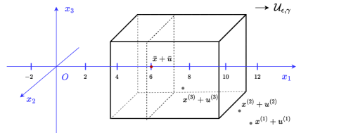
Figure 1: Example of partly smooth set-valued maximally monotone operator and identifiable set.

Example 4.6 ($\ell_{1}$-norm).

To illustrate Theorem 4.3, we consider the following simple example in $\mathbb{R}^{3}$, where $A$ is a maximally monotone operator of the form, for $\forall x\in\mathbb{R}^{3}$

$$A(x)=\mathrm{sign}(x)+\begin{pmatrix}x_{1}-7\\ x_{2}-1/2\\ x_{3}-1/2\end{pmatrix},\,\textrm{where}\,\,\mathrm{sign}(x)=\left\{\begin{aligned} &+1,&x>0,\\ &[-1,1],&x=0,\\ &-1,&x<0.\end{aligned}\right.$$

Apparently for $\bar{x}=[6,0,0]^{\top}$ we have $\bar{u}=0\in\mathrm{ri}(A(\bar{x}))$, and also $A$ is partly smooth along the set $\mathcal{M}=[\mathbb{R},0,0]^{\top}$. Therefore, consider the local union $\mathcal{U}_{\varepsilon,\gamma}$ of $x+A(x)$ of $\bar{x}$ along $\mathcal{M}$ which is shown in Figure 1, clearly, $\mathcal{U}_{\varepsilon,\gamma}$ has full dimension. For the sequence $x^{(k)}+u^{(k)}\to\bar{x}+\bar{u}$, the first two points $x^{(1)}+u^{(1)}$ and $x^{(2)}+u^{(2)}$ are outside $\mathcal{U}_{\varepsilon,\gamma}$, and starting from the 3rd point, $x^{(k)}+u^{(k)}\in\mathrm{int}(\mathcal{U}_{\varepsilon,\gamma})$ and $u^{(k)}\in\mathrm{ri}(A(x^{(k)}))$.

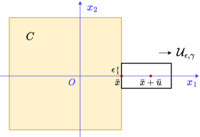
(a) 2D example

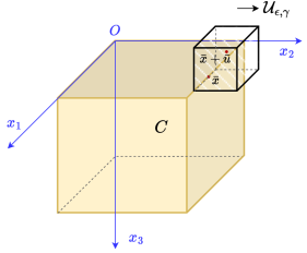
(b) 3D example

Figure 2: Illustrations of local unions for indicator functions. (a) A two-dimensional example. (b) A three-dimensional example.

Example 4.7 (Indicator function).

We now consider indicator function examples, in both $\mathbb{R}^{2}$ and $\mathbb{R}^{3}$. The indicator function is represented as

$$\iota_{C}(x)=\left\{\begin{array}[]{cc}0&,x\in C\\ +\infty&,x\notin C\end{array}\right.$$

As shown in Figure 2, we present two examples of the indicator function $\iota_{C}$, where the set $C$ is represented by the yellow region. We then plot the local union $\mathcal{U}_{\varepsilon,\gamma}$ based on given $\bar{x}$ and $\bar{u}$. Note that according to the definition of the local union, it suffices to consider $u$ within the $\varepsilon$-localization around $\bar{u}$.

Remark 4.8.

From the illustration of $\ell_{1}$-norm, it can be seen that $\mathcal{U}_{\varepsilon,\gamma}$ is a polyhedron. This is due to the fact that the dual norm of $\ell_{1}$-norm is $\ell_{\infty}$-norm. For this case, we can refine the condition in (4.6) by defining the distance function

$$\mathrm{dist}\big{(}{\bar{u},A_{\varepsilon}(x^{(k)})}\big{)}=\inf_{u\in A_{\varepsilon}(x^{(k)})}{|\kern-1.125pt|}\bar{u}-u{|\kern-1.125pt|}_{\infty},$$

instead of the standard $\ell_{2}$-norm distance. This allows to provide a tighter analysis on identification, see Section 5.2.1 for discussion.

For the rest of the section, we need to discuss the following problems: 1) relation with the constant rank property [14]; 2) identifiability without strong inclusion condition A.3; 3) if the sequence $\{x^{(k)}\}_{k\in\mathbb{N}}$ is generated by a numerical scheme, what is the upper bound for the number of steps needed for identification.

4.2 Relation with constant rank property

We investigate the relationship between our definition and the constant rank property of [14]. It can be shown that under the strong inclusion condition, Definition 3.4 naturally leads to the constant rank property, thereby establishing a connection between these two concepts.

We begin by recalling the definition of partly smooth operators via constant rank property [14]. Let $\mathcal{X},\mathcal{U}$ be subsets of $\mathbb{R}^{n}$, define the canonical projection ${\rm proj}:\mathcal{X}\times\mathcal{U}\to\mathcal{X}$ by ${\rm proj}(x,u)=x$.

Definition 4.9 (Constant rank [14]).

A set-valued mapping $A:\mathcal{X}\rightrightarrows\mathcal{U}$ is called partly smooth at a point $\bar{x}\in\mathcal{X}$ for $\bar{u}\in A(\bar{x})$ when the graph $\mathrm{gph}\,(A)$ is a smooth manifold around $(\bar{x},\bar{u})$ and the projection ${\rm proj}$ restricted to $\mathrm{gph}\,(A)$ has constant rank around $(\bar{x},\bar{u})$. The dimension of $A$ at $\bar{x}$ for $\bar{u}$ is then just the dimension of its graph around $(\bar{x},\bar{u})$.

From now on, we use the rank of the projection operator to represent the dimension of the manifold $\mathcal{M}$, which is denoted as $\mathrm{rank}\big{(}{{\rm proj}(\mathrm{gph}\,(A),\,\mathcal{M})}\big{)}$.

Proposition 4.10.

Under the resolvent-regularity condition A.2 and strong inclusion condition A.3, Definition 3.4 implies Definition 4.9.

• As $\mathcal{M}$ is a manifold and $A$ is partly smooth at $\bar{x}$ relative to $\mathcal{M}$, the graph $\mathrm{gph}\,(A)$ locally around $(\bar{x},\bar{u})$ is a manifold. From Proposition 4.5, the resolvent-regularity of $A$ at $\bar{x}$ for $\bar{u}$ ensures locally the uniqueness of $\mathcal{M}$. Define the localization of graph of $A$ as

  $$G_{\varepsilon}=\mathrm{gph}\,(A)\,{\cap}\,\big{(}{{\mathds{B}}_{\varepsilon}(\bar{x})\times{\mathds{B}}_{\varepsilon}(\bar{u})}\big{)},$$

  we have

  $${\rm proj}(G_{\varepsilon})=\mathcal{M}\cap{\mathds{B}}_{\varepsilon}(\bar{x})$$

  which is unique. Hence ${\rm proj}$ has constant rank property around $(\bar{x},\bar{u})$. ∎

4.3 Non-degenrate condition fails

The strong inclusion condition A.3, a.k.a. non-degeneracy condition in optimization, is crucial to the identifiability, as it ensures the uniqueness of the active manifold, which also means the active manifold is “minimal” in terms of dimension.

When A.3 fails, so does (4.4). However, the failure of strong inclusion is not always easy to characterize, take $\ell_{0}$-norm for example, whose subdifferential is unbounded and proximal subdifferential is an open set, see Section 5.1.1. Therefore, in part we focus on the case $A$ is moreover (locally) monotone around $\bar{x}$.

Remark 4.11.

In [8], based on the “mirror stratification” of proper l.s.c. convex functions, the authors studied the identifiability without non-degenerate condition. It is shown that the failure of non-degeneracy results results in an enlarged manifold that contains the minimal true manifold, and identification lands on a layer between the minimal manifold and the enlarged manifold.

With our novel local characterization of identification, we are able to extend the identifiablity to the degenerate setting. Similar to [8], we also need an enlarged manifold, which is provided in the definition below. Recall the definition of the local union $\mathcal{U}_{\varepsilon,\gamma}$ in (4.1), since $A$ is locally monotone around $\bar{x}$, $A$ is resolvent regular at $\bar{x}$ for any $u\in A(\bar{x})$. Define the following local union parameterized by only $\gamma>0$,

$$\mathcal{U}_{\gamma}\stackrel{{\scriptstyle\text{\rm\tiny def}}}{{=}}{\bigcup}_{x\in\mathcal{M}\cap{\mathds{B}}_{\varepsilon}(\bar{x})}\big{(}{x+\gamma A(x)}\big{)},$$

with $\varepsilon>0$ small enough such that $A$ is monotone over ${\mathds{B}}_{\varepsilon}(\bar{x})$.

Definition 4.12 (Enlarged manifold).

Let the set-valued operator $A:\mathbb{R}^{n}\rightrightarrows\mathbb{R}^{n}$ be locally monotone around $\bar{x}$, and partly smooth at $\bar{x}$ relative to a $C^{p}$-manifold $\mathcal{M}\subset\mathbb{R}^{n}$. Let $\bar{u}\in\mathrm{rbd}\big{(}{A(\bar{x})}\big{)}$, then the enlarged manifold for $\bar{u}$ is defined by

$$\widehat{\mathcal{M}}\in\mathrm{argmin}_{\mathrm{rank}({\rm proj}(\mathrm{gph}\,(A),\,\mathcal{M}^{\prime}))}\Big{\{}\mathcal{M}^{\prime}\subset\mathbb{R}^{n}\mid\bar{z}\in\mathrm{int}\big{(}{\mathcal{U}_{\gamma}}\big{)},\,\,\mathcal{M}\subseteq\mathcal{M}^{\prime}\Big{\}},$$

where $\bar{z}=\bar{x}+\gamma\bar{u}$.

We are ready to discuss the identifiability without strong inclusion condition.

Corollary 4.13 (Enlarged identification).

Suppose the set-valued operator $A:\mathbb{R}^{n}\rightrightarrows\mathbb{R}^{n}$ is locally monotone around $\bar{x}$, and partly smooth at $\bar{x}$ relative to a $C^{p}$-manifold $\mathcal{M}\subset\mathbb{R}^{n}$. Given a degenerate dual vector

$$\bar{u}\in\mathrm{rbd}\big{(}{A(\bar{x})}\big{)}.$$

There exists an enlarged manifold $\widehat{\mathcal{M}}$ such that

$$\widehat{\mathcal{U}}_{\gamma}\stackrel{{\scriptstyle\text{\rm\tiny def}}}{{=}}{\bigcup}_{x\in\widehat{\mathcal{M}}\cap{\mathds{B}}_{\varepsilon}(\bar{x})}\big{(}{x+\gamma A(x)}\big{)}$$

has full dimension. If, moreover, $A$ is continuous at $\bar{x}$ relative $\widehat{\mathcal{M}}$, then $\widehat{\mathcal{M}}$ is identifiable at $\bar{x}$ for $\bar{u}$.

The above identifiability is the direct consequence of Theorem 4.3.

Remark 4.14.

Though we can obtain identifiabilty, the identified manifold is no longer unique. In terms of the dimension of the identified manifold, it can be euqal to that of $\mathcal{M}$ or $\widehat{\mathcal{M}}$, or something between. In Section 5.2.2, we provide examples to illustrate this.

4.4 Upper bound for identificaton steps

In either the previous result, Proposition 3.2, or our Theorem 4.3, it is only stated that for $k$ large enough, manifold identification occurs. However, the estimation of this $k$ is not provided. This problem has been considered in the literature, such as [21, 32]. Based on new local characterization, we are able to provide a new estimation.

For the sake of simplicity, our following discussion assumes the dual vector is convergent.

Proposition 4.15.

Let the set-valued operator $A:\mathbb{R}^{n}\rightrightarrows\mathbb{R}^{n}$ be partly smooth at $\bar{x}$ relative to a manifold $\mathcal{M}\subset\mathbb{R}^{n}$, and $r$-resolvent-regular at $\bar{x}$ for $\bar{u}\in\mathrm{rbd}\big{(}{A_{\varepsilon}(\bar{x})}\big{)}$. Let $K>0$ be such that

$${|\kern-1.125pt|}(x^{(k)}+\gamma u^{(k)})-(\bar{x}+\gamma\bar{u}){|\kern-1.125pt|}\leq d\stackrel{{\scriptstyle\text{\rm\tiny def}}}{{=}}\mathrm{dist}\big{(}{\bar{x}+\gamma\bar{u},\,\mathcal{U}_{\varepsilon,\gamma}}\big{)}$$

holds for all $k\geq K$, then

$$x^{(k)}\in\mathcal{M},\,\forall k\geq K.$$

In particular, if there exists $p>0$ such that for any $k\in\mathbb{N}$,

$${|\kern-1.125pt|}u^{(k)}-\bar{u}{|\kern-1.125pt|}\leq p{|\kern-1.125pt|}x^{(k)}-\bar{x}{|\kern-1.125pt|}.$$ (4.13)

Then we have

1. If $L=\sum_{k\in\mathbb{N}}{|\kern-1.125pt|}x^{(k)}-x^{(k-1)}{|\kern-1.125pt|}<+\infty$, then

   $$K=\mathrm{argmin}_{k}\left\{k\geq 0\mid\sum_{i=0}^{k-1}{|\kern-1.125pt|}x^{(i)}-x^{(i+1)}{|\kern-1.125pt|}\geq L-{{\frac{\raisebox{1.24994pt}{\small$d$}}{\raisebox{-2.08333pt}{\small$1+\gamma p$}}}}\right\}.$$

2. If ${|\kern-1.125pt|}x^{(k)}-\bar{x}{|\kern-1.125pt|}\leq C\rho^{k}$ for some $C>0$ and $\rho\in]0,1[$, then

   $$K=\left\lceil\frac{\log d-\log(1+\gamma p)-\log C}{\log\rho}\right\rceil,$$

   where $\lceil q\rceil,\,q\in\mathbb{R}$ denotes the smallest integer that is larger than $q$.

• Note that if

  $${|\kern-1.125pt|}(x^{(k)}+\gamma u^{(k)})-(\bar{x}+\gamma\bar{u}){|\kern-1.125pt|} \leq{|\kern-1.125pt|}x^{(k)}-\bar{x}{|\kern-1.125pt|}+\gamma{|\kern-1.125pt|}u^{(k)}-\bar{u}{|\kern-1.125pt|}$$

  $$\leq(1+\gamma p){|\kern-1.125pt|}x^{(k)}-\bar{x}{|\kern-1.125pt|}$$

  $$\leq d,$$

  identification happens owing to Theorem 4.3.

  1. The finite sum $L=\sum_{k\in\mathbb{N}}{|\kern-1.125pt|}x^{(k)}-x^{(k-1)}{|\kern-1.125pt|}<+\infty$ means the sequence $\{x^{(k)}\}_{k\in\mathbb{N}}$ has finite length. Therefore, given $K>0$, if we let

     $$(1+\gamma p){|\kern-1.125pt|}x^{(K)}-\bar{x}{|\kern-1.125pt|} \leq(1+\gamma p)\sum_{i=K}^{\infty}{|\kern-1.125pt|}x^{(i)}-x^{(i+1)}{|\kern-1.125pt|}$$

     $$\leq(1+\gamma p)\left({L-\sum_{i=0}^{K-1}{|\kern-1.125pt|}x^{(i)}-x^{(i+1)}{|\kern-1.125pt|}}\right)\leq d,$$

     then we have

     $$\sum_{i=0}^{K-1}{|\kern-1.125pt|}x^{(i)}-x^{(i+1)}{|\kern-1.125pt|}\geq L-{{\frac{\raisebox{1.24994pt}{\small$d$}}{\raisebox{-2.08333pt}{\small$1+\gamma p$}}}}.$$

     Let $K$ be the smallest integer such that the above inequality holds, then we prove the claim.

  2. The second case is much more straight as $x^{(k)}$ converges linearly. As a result, if $K$ is large enough such that

     $$(1+\gamma p){|\kern-1.125pt|}x^{(K)}-\bar{x}{|\kern-1.125pt|}\leq(1+\gamma p)\times C\rho^{K} \leq d,$$

     then identification happens and we have

     $$K\geq\frac{\log d-\log(1+\gamma p)-\log C}{\log\rho}.$$

     Taking the smallest integer larger than the lhs of the above inequality concludes the proof. ∎

Remark 4.16.

 

• Condition (4.13) is algorithm dependent, see Example 4.17 for an illustration of Forward–Backward splitting method.

• In general, in the context of non-smooth optimization or monotone inclusion, when only a sublinear convergence rate is achieved, it is typically expressed in terms of the residual ${|\kern-1.125pt|}x^{(k)}-x^{(k-1)}{|\kern-1.125pt|}$ rather than ${|\kern-1.125pt|}x^{(k)}-\bar{x}{|\kern-1.125pt|}$, unless stronger assumptions are imposed [19]. However, finite length property exists in for many problems, such as nonsmooth optimization with objective satisfying Kurdyka–Łojasiewicz inequality. Another example is the FISTA method; as shown in [23], a modified version achieves the following convergence rate

  $$\sum_{k\in\mathbb{N}}k{|\kern-1.125pt|}x^{(k)}-x^{(k+1)}{|\kern-1.125pt|}^{2}<+\infty,$$

  which is analog to finite length.

• Under degeneracy condition, we can also provide an upper bound estimation of identification step as stated in Proposition 4.15.

Below we use Forward–Backward splitting method to illustrate Proposition 4.15.

Example 4.17.

Consider the following monotone inclusion

$${\rm find}\quad x\in\mathbb{R}^{n}\quad{\rm such\,that\,}\quad 0\in A(x)+B(x),$$ (4.14)

where $A:\mathbb{R}^{n}\rightrightarrows\mathbb{R}^{n}$ is a maximally monotone and $B:\mathbb{R}^{n}\to\mathbb{R}^{n}$ is a $\beta$-cocoercive operator with $\beta>0$. Let $\{x^{(k)}\}_{k\in\mathbb{N}}$ be the sequence generated from the Forward-Backward splitting method [24]

$$x^{(k+1)}=\mathscr{J}_{\gamma A}(\mathrm{Id}-\gamma B)(x^{(k)}),\,\,\gamma\in]0,2\beta[.$$

1. Let $\bar{x}$ be a solution of (4.14), then

   $$\bar{x}=\mathscr{J}_{\gamma A}(\mathrm{Id}-\gamma B)(\bar{x})$$

   and denote $\bar{u}=-B(\bar{x})$.

2. If $B$ is strongly monotone with modulus $\kappa>0$, that is

   $$\langle B(x)-B(y),\,x-y\rangle\geq\kappa{|\kern-1.125pt|}x-y{|\kern-1.125pt|}^{2}.$$

   Since $\mathscr{J}_{\gamma A}$ is firmly nonexpansive, we have

   $${|\kern-1.125pt|}x^{(k+1)}-\bar{x}{|\kern-1.125pt|}^{2} ={|\kern-1.125pt|}\mathscr{J}_{\gamma A}(\mathrm{Id}-\gamma B)(x^{(k)})-\mathscr{J}_{\gamma A}(\mathrm{Id}-\gamma B)(\bar{x}){|\kern-1.125pt|}^{2}$$

   $$\leq{|\kern-1.125pt|}(\mathrm{Id}-\gamma B)(x^{(k)})-(\mathrm{Id}-\gamma B)(\bar{x}){|\kern-1.125pt|}^{2}$$

   $$\leq{|\kern-1.125pt|}x^{(k)}-\bar{x}{|\kern-1.125pt|}^{2}-2\gamma\langle x^{(k)}-\bar{x},\,B(x^{(k)})-B(\bar{x})\rangle+\gamma^{2}{|\kern-1.125pt|}B(x^{(k)})-B(\bar{x}){|\kern-1.125pt|}^{2}$$

   $$\leq\big{(}{1-2\gamma\kappa+{{\frac{\raisebox{0.41669pt}{\footnotesize$\gamma^{2}$}}{\raisebox{-1.24994pt}{\footnotesize$\beta^{2}$}}}}}\big{)}{|\kern-1.125pt|}x^{(k)}-\bar{x}{|\kern-1.125pt|}^{2}.$$

   When $\gamma(2\kappa-\gamma/\beta^{2})\in]0,1[$, then $\rho^{2}=1-\gamma(2\kappa-{{\frac{\raisebox{0.29167pt}{\footnotesize$\gamma$}}{\raisebox{-0.87495pt}{\footnotesize$\beta^{2}$}}}})<1$ and

   $${|\kern-1.125pt|}x^{(k)}-x^{\star}{|\kern-1.125pt|}\leq\rho^{k}{|\kern-1.125pt|}x^{(0)}-\bar{x}{|\kern-1.125pt|}.$$

3. The update of $x^{(k)}$ yields the dual vector

   $$u^{(k)}={{\frac{\raisebox{1.24994pt}{\small$x^{(k-1)}-x^{(k)}$}}{\raisebox{-2.08333pt}{\small$\gamma$}}}}-B(x^{(k-1)})\in A(x^{(k)}).$$

   Then we have

   $${|\kern-1.125pt|}u^{(k)}-\bar{u}{|\kern-1.125pt|} ={|\kern-1.125pt|}{{\frac{\raisebox{0.41669pt}{\footnotesize$x^{(k-1)}-x^{(k)}$}}{\raisebox{-1.24994pt}{\footnotesize$\gamma$}}}}-B(x^{(k-1)})+B(\bar{x}){|\kern-1.125pt|}$$

   $$={{\frac{\raisebox{0.41669pt}{\footnotesize$1$}}{\raisebox{-1.24994pt}{\footnotesize$\gamma$}}}}{|\kern-1.125pt|}\bar{x}-x^{(k)}+x^{(k-1)}-\gamma B(x^{(k-1)})-\bar{x}+\gamma B(\bar{x}){|\kern-1.125pt|}$$

   $$\leq{{\frac{\raisebox{0.41669pt}{\footnotesize$1$}}{\raisebox{-1.24994pt}{\footnotesize$\gamma$}}}}\big{(}{{|\kern-1.125pt|}x^{(k)}-\bar{x}{|\kern-1.125pt|}+{|\kern-1.125pt|}x^{(k-1)}-\bar{x}{|\kern-1.125pt|}}\big{)}$$

   $$\leq{{\frac{\raisebox{0.41669pt}{\footnotesize$2$}}{\raisebox{-1.24994pt}{\footnotesize$\gamma$}}}}{|\kern-1.125pt|}x^{(k-1)}-\bar{x}{|\kern-1.125pt|}$$

   $$\leq{{\frac{\raisebox{0.41669pt}{\footnotesize$2$}}{\raisebox{-1.24994pt}{\footnotesize$\gamma$}}}}{|\kern-1.125pt|}x^{(0)}-\bar{x}{|\kern-1.125pt|}\rho^{k-1}.$$

   Consequently,

   $${|\kern-1.125pt|}x^{(k)}-\bar{x}{|\kern-1.125pt|}+\gamma{|\kern-1.125pt|}u^{(k)}-\bar{u}{|\kern-1.125pt|} \leq\rho^{k}{|\kern-1.125pt|}x^{(0)}-\bar{x}{|\kern-1.125pt|}+2{|\kern-1.125pt|}x^{(0)}-\bar{x}{|\kern-1.125pt|}\rho^{k-1}$$

   $$\leq\rho^{k}\times\big{(}{{|\kern-1.125pt|}x^{(0)}-\bar{x}{|\kern-1.125pt|}+{{\frac{\raisebox{0.41669pt}{\footnotesize$2$}}{\raisebox{-1.24994pt}{\footnotesize$\rho$}}}}{|\kern-1.125pt|}x^{(0)}-\bar{x}{|\kern-1.125pt|}}\big{)}.$$

   By making $\rho^{k}\times\big{(}{1+{{\frac{\raisebox{0.29167pt}{\footnotesize$2$}}{\raisebox{-0.87495pt}{\footnotesize$\rho$}}}}}\big{)}{|\kern-1.125pt|}x^{(0)}-\bar{x}{|\kern-1.125pt|}<d$, we can obtain the estimation of $K$.

Remark 4.18.

We can also consider the error bound condition or strong metric regularity [7] in Example 4.17, both of which are weaker than strong monotonicity. However, these conditions can still yield similar estimates for the identification step, differing only in the associated parameter.

5 Applications

In this section, we provide various examples to verify our theoretical findings. 1) We first discuss examples of partly smooth operators, including the (limiting) subdifferential of $\ell_{0}$-norm, monotone inclusion formulation of Primal–Dual splitting which is also discussed in [14], and variational inequality. 2) Then we verify the result of identification under nonconvergent dual vector via mini-batch stochastic gradient descent, and under degenerate dual vector via proximal operator of $\ell_{1}$-norm. 3) Lastly, we verify the upper bound of number of steps for identification via elastic net.

5.1 Examples of partly smooth set-valued operators

In this part, we provide three examples of partly smooth operators, one is the subdifferential of nonconvex function, while the other is monotone operators from Primal–Dual splitting method and variational inequality.

5.1.1 Subdifferential of nonconvex function

As subdifferential is an important source of set-valued operators, when a function is partly smooth, its (limiting) subdifferential is also partly smooth. For convex partly smooth functions, the results in Section 4 are quite straightforward to verify as all the regularity conditions are satisfied automatically; we refer to [18] for convex examples. For subdifferential of nonconvex function, the local characterization is controlled by the (prox-)regularity, below we provide an example of $\ell_{0}$-norm.

Example 5.1 ($\ell_{0}$-norm).

For $x\in\mathbb{R}^{n}$, the $\ell_{0}$-norm of $x$ is defined as

$$f(x)={|\kern-1.125pt|}x{|\kern-1.125pt|}_{0}\stackrel{{\scriptstyle\text{\rm\tiny def}}}{{=}}\#\big{\{}i:x_{i}\neq 0\big{\}},$$

which returns the number of nonzero element in $x$. It can verified that $R$ is a polyhedral norm, given $\bar{x}\in\mathbb{R}^{n}$, denote $\mathcal{S}=\{i:\bar{x}_{i}\neq 0\}$, then $\ell_{0}$-norm is partly smooth at $\bar{x}$ relative to the following manifold

$$\mathcal{M}=\big{\{}x\in\mathbb{R}^{n}\mid\mathrm{supp}(x)\subseteq\mathcal{S}\big{\}},$$

which is a subspace. Therefore, the tangent space of $\mathcal{M}$ at $\bar{x}$ is $\mathcal{M}$ itself, i.e. $\mathcal{T}_{\mathcal{M}}(\bar{x})=\mathcal{M}$. Denote $\mathcal{S}^{\bot}=\big{\{}1,...,n\big{\}}\setminus\mathcal{S}$ the complement of the $\mathcal{S}$, the subdifferential at $\bar{x}$ then is

$$\partial f(\bar{x})=\mathrm{span}\big{\{}e_{i},\,i\in\mathcal{S}^{\bot}\big{\}},$$

where $e_{i}$ is the $i$’th standard normal basis of $\mathbb{R}^{n}$.

For the sake of simplicity, for the discussion below we let $n=2$ and $\bar{x}=\begin{bmatrix}1&0\end{bmatrix}^{\top}$. For this setting, we have

$$\mathcal{M}=\mathcal{T}_{\mathcal{M}}(\bar{x})=\begin{bmatrix}\mathbb{R}\\ 0\end{bmatrix}\enskip\text{and}\enskip\partial f(\bar{x})=\begin{bmatrix}0\\ \mathbb{R}\end{bmatrix}.$$

Given $\varepsilon>0$ and $\gamma>0$, define

$${\mathcal{U}} ={\bigcup}_{x\in\mathcal{M}\cap{\mathds{B}}_{\varepsilon}(\bar{x})}\big{(}{x+\gamma\partial f(x)}\big{)}=\begin{bmatrix}[1-\varepsilon,1+\varepsilon]\\ \mathbb{R}\end{bmatrix}.$$

It is clear that $\mathrm{par}({\mathcal{U}})=\mathbb{R}^{2}$. However, $\mathrm{prox}_{\gamma f}(\mathcal{U})\neq\mathcal{M}\cap{\mathds{B}}_{\varepsilon}(\bar{x})$ as $\mathcal{U}$ is unbounded and regularity is not considered. Let $\bar{u}=\begin{bmatrix}0&0\end{bmatrix}^{\top}\in\partial f(\bar{x})$, then it can be verified that $f$ is $r$-prox-regular at $\bar{x}$ for $\bar{u}$ for some $r>0$. Denote $(\partial f)_{\varepsilon}$ the localization of $\partial f$, let $\gamma\in]0,1/r[$ and define

$${\mathcal{U}_{\varepsilon,\gamma}} ={\bigcup}_{x\in\mathcal{M}\cap{\mathds{B}}_{\varepsilon}(\bar{x})}\big{(}{x+\gamma(\partial f)_{\varepsilon}(x)}\big{)}=\begin{bmatrix}[1-\varepsilon,1+\varepsilon]\\ [-\gamma\varepsilon,\gamma\varepsilon]\end{bmatrix}.$$

Given that $\gamma\varepsilon\leq\sqrt{2\gamma}<1-\varepsilon$, we have

$$\mathrm{prox}_{\gamma f}(\mathcal{U}_{\varepsilon,\gamma})=\mathcal{M}\cap{\mathds{B}}_{\varepsilon}(\bar{x}).$$

Suppose now we have a sequence $\{x^{(k)}\}_{k\in\mathbb{N}}$ with $x^{(k)}\to\bar{x}$ and $\partial f(x^{(k)})\ni u^{(k)}\to\bar{u}$, then necessarily for all $k$ large enough, we have

$$u^{(k)}\in(\partial f)_{\varepsilon}(x^{(k)})\enskip\text{and}\enskip x^{(k)}+\gamma u^{(k)}\in\mathcal{U}_{\varepsilon,\gamma}.$$

As a result $x^{(k)}\in\mathcal{M}\cap{\mathds{B}}_{\varepsilon}(\bar{x})$.

5.1.2 Primal-Dual splitting

The second example we consider is the Primal-Dual splitting method [4, 5], the convergence property of the method under partial smoothness is studied in [22], later on in [14] it is used an example of partly smooth operators. For the sake of completeness, we provide the derivation here as an example of partly smooth operator which is not the subdifferential of partly smooth functions.

Consider the following saddle point problem

$$\min_{x\in\mathbb{R}^{n}}\max_{y\in\mathbb{R}^{m}}\,f(x)+p(x)+\langle Kx,y\rangle-g^{*}(y)-q^{*}(y)$$ (5.1)

where

• $K:\mathbb{R}^{n}\to\mathbb{R}^{m}$ is a bounded linear operator.

• $f:\mathbb{R}^{n}\to\bar{\mathbb{R}}$ and $g:\mathbb{R}^{m}\to\bar{\mathbb{R}}$ are proper l.s.c. and convex functions.

• $p:\mathbb{R}^{n}\to\mathbb{R}$ is convex differentiable with $\beta_{p}$-Lipschitz continuous gradient.

• $q^{*}:\mathbb{R}^{m}\to\mathbb{R}$ is convex differentiable with $\beta_{q^{*}}$-Lipschitz continuous gradient

Given a saddle point $(\bar{x},\bar{y})$, the associated optimality condition reads

$$0 \in\partial f(\bar{x})+\nabla p(\bar{x})+K^{\top}\bar{y},$$

$$0 \in-K\bar{x}+\partial g^{*}(\bar{y})+\nabla q^{*}(\bar{y}),$$

which can be written as

$$0\in\underbrace{\begin{bmatrix}\partial f&K^{\top}\\ -K&\partial g^{*}\end{bmatrix}}_{A}\begin{bmatrix}\bar{x}\\ \bar{y}\end{bmatrix}+\underbrace{\begin{bmatrix}\nabla p&0\\ 0&\nabla q^{*}\end{bmatrix}}_{B}\begin{bmatrix}\bar{x}\\ \bar{y}\end{bmatrix}.$$ (5.2)

Where $A$ is maximally monotone and $B$ is co-coercive. By denoting $z=\begin{bmatrix}x\\ y\end{bmatrix}$, the original problem (5.1) is equivalent to solve the following monotone inclusion problem

$${\rm find}\quad z\in\mathbb{R}^{n}\times\mathbb{R}^{m}\quad{\rm such\,that}\quad 0\in A(z)+B(z).$$ (5.3)

Note that $A$ has the decomposition

$$A=\begin{bmatrix}\partial f&0\\ 0&\partial g^{*}\end{bmatrix}+\begin{bmatrix}0&K^{\top}\\ -K&0\end{bmatrix}.$$

Hence according Proposition 3.6 and Corollary 3.12, we have the following result regarding the partial smoothness of $A$.

Proposition 5.2.

For the optimization problem (5.1), given a saddle point $(\bar{x},\bar{y})$ suppose the following holds

• $f$ is partly smooth at $\bar{x}$ relative to $\mathcal{M}_{\bar{x}}$;

• $g^{*}$ is partly smooth at $\bar{y}$ relative $\mathcal{M}_{\bar{y}}$;

Then the set-valued operator $A$ in (5.2) is partly smooth.

5.1.3 Variational inequalities

Examples of partly smooth operators also arise from variational inequalities. First, consider the following optimization problem with linear constraint

$$\min_{x\in\mathbb{R}^{n},\,y\in\mathbb{R}^{m}} f(x)+g(y)$$ (5.4)

$${\rm subject\,to} Cx+Dy=e,$$

where the following assumptions are imposed

• $f:\mathbb{R}^{n}\to\bar{\mathbb{R}}$ and $g:\mathbb{R}^{m}\to\bar{\mathbb{R}}$ are proper l.s.c. and convex functions.

• $C:\mathbb{R}^{n}\to\mathbb{R}^{\ell},\,D:\mathbb{R}^{m}\to\mathbb{R}^{\ell}$ are bounded linear operators.

We also assume that the problem is well-posed such that solution exists. Let $\lambda$ be the dual vector, then the Lagrangian associated to (5.4) reads

$$\mathcal{L}(x,y,\lambda)=f(x)+g(y)-\langle\lambda,\,Cx+Dy-e\rangle.$$

Let $(\bar{x},\bar{y})$ and $\bar{\lambda}$ be primal and dual optimal, then there holds

$$\langle x-\bar{x},\,\tilde{\nabla}f(\bar{x})-C^{\top}\bar{\lambda}\rangle \geq 0,\,\,\,\forall x\in\mathbb{R}^{n}\enskip\text{and}\enskip\tilde{\nabla}f(\bar{x})\in\partial f(\bar{x}),$$ (5.5)

$$\langle y-\bar{y},\,\tilde{\nabla}g(\bar{y})-D^{\top}\bar{\lambda}\rangle \geq 0,\,\,\,\forall y\in\mathbb{R}^{m}\enskip\text{and}\enskip\tilde{\nabla}g(\bar{y})\in\partial g(\bar{x}),$$

$$\langle\lambda-\bar{\lambda},\,C\bar{x}+D\bar{y}-e\rangle \geq 0,\,\,\,\forall\lambda\in\mathbb{R}^{\ell}.$$

Denote $\mathcal{Z}=\mathbb{R}^{n}\times\mathbb{R}^{m}\times\mathbb{R}^{m}$,

$$z=\begin{bmatrix}x\\ y\\ \lambda\end{bmatrix}\enskip\text{and}\enskip A(z)=\begin{bmatrix}\partial f(x)-C^{\top}\lambda\\ \partial g(y)-D^{\top}\lambda\\ Cx+Dy-e\end{bmatrix}.$$

Note that $A$ is maximally monotone. Then solving the optimization problem is equivalent to solving the follow variational inequality

$$\langle z-\bar{z},\,\bar{w}\rangle\geq 0,\ \,\textrm{ for }\,\forall z\in\Omega\enskip\text{and}\enskip\bar{w}\in A(\bar{z}).$$ (5.6)

Similar to the case of Primal-Dual splitting method, under partial smoothness assumptions of $f$ and $g$, the set-valued operator $A$ is partly smooth.

5.2 Identification properties and iteration bounds

In this part, we turn to the identification property of partial smoothness and discuss its behavior under much weaker conditions compared to the existing result. We first discuss the identification result under the setting that the dual vector is not convergent using proximal mini-batch stochastic gradient, then we discuss the scenario where the non-degeneracy condition fails. We conclude this part by check the upper bound on the number of iterations need for identification.

5.2.1 Identification with non-convergent dual vector

Consider the following LASSO regression problem

$$\min_{x\in\mathbb{R}^{n}}\,\mu{|\kern-1.125pt|}x{|\kern-1.125pt|}_{1}+{{\frac{\raisebox{1.24994pt}{\small$1$}}{\raisebox{-2.08333pt}{\small$m$}}}}\sum\nolimits_{i=1}^{m}{{\frac{\raisebox{0.41669pt}{\footnotesize$1$}}{\raisebox{-1.24994pt}{\footnotesize$2$}}}}(a_{i}^{\top}x-b_{i})^{2},$$ (5.7)

where for each $i=1,...,m$, $a_{i}$ is random Gaussian vector, and $b_{i}$ is generated via

$$b_{i}=a_{i}^{\top}\tilde{x}+\epsilon_{i},\,\,\epsilon\sim\mathcal{N}(0,\sigma^{2}),$$

for some $\sigma>0$, and $\tilde{x}$ is a $\kappa$-sparse vector with $\kappa<m$.

The algorithm We solve the problem with proximal mini-batch stochastic gradient method [30], with fixed batch size $s$. The iteration of the algorithms is described below:

$$\left\lfloor\begin{aligned} &\textrm{Sample the index subset $\mathcal{I}_{k}\subset\big{\{}1,2,...,m\big{\}}$ with size $s$},\\[2.84526pt] &\,x^{(k+1)}=\mathrm{prox}_{\mu\alpha_{k}{|\kern-1.125pt|}\cdot{|\kern-1.125pt|}_{1}}{\big{(}}{x^{(k)}-{{\frac{\raisebox{1.49994pt}{\small$\alpha_{k}$}}{\raisebox{-2.5pt}{\small$s$}}}}\mathbin{\scalebox{1.25}{$\sum$}}_{i\in\mathcal{I}_{k}}\big{(}{a_{i}^{\top}x^{(k)}-b_{i}}\big{)}a_{i}}{\big{)}},\end{aligned}\right.$$

where $\alpha_{k}$ is step-size. It is well-known that stochastic gradient has non-vanishing error (or bounded variance), see below for a simple derivation, this is the reason why proximal stochastic gradient descent does not have identification property as pointed out in [29]. However, when mini-batch is considered, with Theorem 4.3 the new condition for identification, we can show that identification occurs when batch size is large enough.

Dual vector From the definition of proximal operator, we have

$$u^{(k+1)}\stackrel{{\scriptstyle\text{\rm\tiny def}}}{{=}}{{\frac{\raisebox{1.24994pt}{\small$x^{(k)}-x^{(k+1)}$}}{\raisebox{-2.08333pt}{\small$\mu\alpha_{k}$}}}}-{{\frac{\raisebox{1.24994pt}{\small$1$}}{\raisebox{-2.08333pt}{\small$s\mu$}}}}\sum\nolimits_{i\in\mathcal{I}_{k}}\big{(}{a_{i}^{\top}x^{(k)}-b_{i}}\big{)}a_{i}\in\partial{|\kern-1.125pt|}x^{(k+1)}{|\kern-1.125pt|}_{1}.$$

For simplicity, assume the solution, denoted as $\bar{x}$, is unique, and denote

$$\bar{u}\stackrel{{\scriptstyle\text{\rm\tiny def}}}{{=}}-{{\frac{\raisebox{1.24994pt}{\small$1$}}{\raisebox{-2.08333pt}{\small$m\mu$}}}}\sum\nolimits_{i=1}^{m}\big{(}{a_{i}^{\top}\bar{x}-b_{i}}\big{)}a_{i}\in\partial{|\kern-1.125pt|}\bar{x}{|\kern-1.125pt|}_{1}.$$

Then $\ell_{1}$-norm is partly smooth at $\bar{x}$ for $\bar{u}$ relative to $\mathcal{M}=\mathbb{R}\mathrm{supp}(\bar{x})$.

Local union Since we are in the convex setting, $\partial{|\kern-1.125pt|}\cdot{|\kern-1.125pt|}_{1}$ is maximal monotone. For some small enough $\varepsilon>0$, the local union

$$\mathcal{U}\stackrel{{\scriptstyle\text{\rm\tiny def}}}{{=}}{\bigcup}_{x\in\mathcal{M}\cap{\mathds{B}}_{\varepsilon}(\bar{x})}\big{(}{x+\partial{|\kern-1.125pt|}x{|\kern-1.125pt|}_{1}}\big{)},$$

has full dimension. Denote the distance

$$d=\mathrm{dist}\big{(}{\bar{x}+\bar{u},\mathrm{bdy}(\mathcal{U})}\big{)}.$$

Under non-degeneracy, we have $d>0$.

Error of the dual vector With the above preparation, denote $\mathcal{I}_{k}^{\bot}$ the complement of $\mathcal{I}_{k}$, then

$${|\kern-1.125pt|}(x^{(k+1)}+u^{(k+1)})-(\bar{x}+\bar{u}){|\kern-1.125pt|}$$ (5.8)

$$\leq{|\kern-1.125pt|}x^{(k+1)}-\bar{x}{|\kern-1.125pt|}+{|\kern-1.125pt|}u^{(k+1)}-\bar{u}{|\kern-1.125pt|}$$

$$\leq{|\kern-1.125pt|}x^{(k+1)}-\bar{x}{|\kern-1.125pt|}+{|\kern-1.125pt|}{{\frac{\raisebox{0.41669pt}{\footnotesize$x^{(k)}-x^{(k+1)}$}}{\raisebox{-1.24994pt}{\footnotesize$\mu\alpha_{k}$}}}}-{{\frac{\raisebox{0.41669pt}{\footnotesize$1$}}{\raisebox{-1.24994pt}{\footnotesize$s\mu$}}}}\mathbin{\scalebox{1.25}{$\sum$}}_{i\in\mathcal{I}_{k}}(a_{i}^{\top}x^{(k)}-b_{i})a_{i}+{{\frac{\raisebox{0.41669pt}{\footnotesize$1$}}{\raisebox{-1.24994pt}{\footnotesize$m\mu$}}}}\mathbin{\scalebox{1.25}{$\sum$}}_{i=1}^{m}(a_{i}^{\top}x^{(k)}-b_{i})a_{i}{|\kern-1.125pt|}$$

$$\leq{|\kern-1.125pt|}x^{(k+1)}-\bar{x}{|\kern-1.125pt|}+{{\frac{\raisebox{0.41669pt}{\footnotesize$1$}}{\raisebox{-1.24994pt}{\footnotesize$\mu\alpha_{k}$}}}}{|\kern-1.125pt|}x^{(k)}-x^{(k+1)}{|\kern-1.125pt|}+{{\frac{\raisebox{0.41669pt}{\footnotesize$1$}}{\raisebox{-1.24994pt}{\footnotesize$\mu$}}}}{|\kern-1.125pt|}{{\frac{\raisebox{0.41669pt}{\footnotesize$m-s$}}{\raisebox{-1.24994pt}{\footnotesize$ms$}}}}\mathbin{\scalebox{1.25}{$\sum$}}_{i\in\mathcal{I}_{k}}a_{i}^{\top}(x^{(k)}-\bar{x})a_{i}-{{\frac{\raisebox{0.41669pt}{\footnotesize$1$}}{\raisebox{-1.24994pt}{\footnotesize$m$}}}}\mathbin{\scalebox{1.25}{$\sum$}}_{i\in\mathcal{I}_{k}^{\bot}}(a_{i}^{\top}x^{(k)}-b_{i})a_{i}{|\kern-1.125pt|}$$

$$\leq{|\kern-1.125pt|}x^{(k+1)}-\bar{x}{|\kern-1.125pt|}+{{\frac{\raisebox{0.41669pt}{\footnotesize$1$}}{\raisebox{-1.24994pt}{\footnotesize$\mu\alpha_{k}$}}}}{|\kern-1.125pt|}x^{(k)}-x^{(k+1)}{|\kern-1.125pt|}+{{\frac{\raisebox{0.41669pt}{\footnotesize$m-s$}}{\raisebox{-1.24994pt}{\footnotesize$\mu ms$}}}}{|\kern-1.125pt|}\mathbin{\scalebox{1.25}{$\sum$}}_{i\in\mathcal{I}_{k}}a_{i}^{\top}(x^{(k)}-\bar{x})a_{i}{|\kern-1.125pt|}+{{\frac{\raisebox{0.41669pt}{\footnotesize$1$}}{\raisebox{-1.24994pt}{\footnotesize$\mu m$}}}}{|\kern-1.125pt|}\mathbin{\scalebox{1.25}{$\sum$}}_{i\in\mathcal{I}_{k}^{\bot}}(a_{i}^{\top}x^{(k)}-b_{i})a_{i}{|\kern-1.125pt|}.$$

Suppose the problem is good enough and the step-size $\alpha_{k}$ is chosen such that $x^{(k)}\to\bar{x}$ and

$${{\frac{\raisebox{0.41669pt}{\footnotesize$1$}}{\raisebox{-1.24994pt}{\footnotesize$\alpha_{k}$}}}}{|\kern-1.125pt|}x^{(k)}-x^{(k+1)}{|\kern-1.125pt|}\to 0.$$

Then for the last line of (5.8), only the last term matters and for which we further for all $k$ large enough

$${{\frac{\raisebox{0.41669pt}{\footnotesize$1$}}{\raisebox{-1.24994pt}{\footnotesize$\mu m$}}}}{|\kern-1.125pt|}\mathbin{\scalebox{1.25}{$\sum$}}_{i\in\mathcal{I}_{k}^{\bot}}(a_{i}^{\top}x^{(k)}-b_{i})a_{i}{|\kern-1.125pt|}\approx{{\frac{\raisebox{0.41669pt}{\footnotesize$1$}}{\raisebox{-1.24994pt}{\footnotesize$\mu m$}}}}{|\kern-1.125pt|}\mathbin{\scalebox{1.25}{$\sum$}}_{i\in\mathcal{I}_{k}^{\bot}}(a_{i}^{\top}\bar{x}-b_{i})a_{i}{|\kern-1.125pt|}>0.$$

This means that if the batch size is chosen large enough such that

$${{\frac{\raisebox{0.41669pt}{\footnotesize$1$}}{\raisebox{-1.24994pt}{\footnotesize$\mu m$}}}}{|\kern-1.125pt|}\mathbin{\scalebox{1.25}{$\sum$}}_{i\in\mathcal{I}_{k}^{\bot}}(a_{i}^{\top}\bar{x}-b_{i})a_{i}{|\kern-1.125pt|}<d$$ (5.9)

holds for all possible $\mathcal{I}_{k}$, we have identification. Note that (5.9) can be used to derive an estimation of minimal batch size needed for identification, however it is not an easy task as computing over all possible $\mathcal{I}_{k}$ is combinatorial and also requires the information of $\bar{x}$.

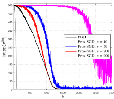
(a) Identification v.s. batch size

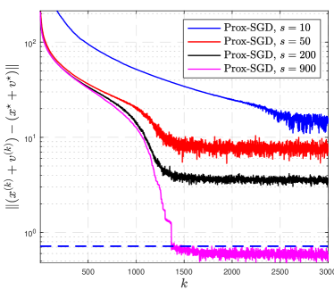
(b) The green dashed line is the estimation of $\mathrm{dist}(\bar{x}+\bar{v},\,\mathcal{U})$

Figure 3: Identification of proximal mini-batch stochastic gradient, and dual vector error.

To illustrate our result, we conduct experiment with a problem size of $(m,n)=(1000,500)$. The identification results for different batch sizes are presented in Figure 3 (a), proximal gradient descent is added for reference. We can observe from the figure that

• When the batch size is small, e.g. $s=10$, no identification happens. Increase the batch size can significantly reduce the support size of $x^{(k)}$.

• For batch size equals $150,900$, we have identification.

We also provide the plot for error ${|\kern-1.125pt|}(x^{(k)}+u^{(k)})-(\bar{x}+\bar{u}){|\kern-1.125pt|}$, as showed in Figure 3 (b):

• The blue dashed line is the estimation of $d=\mathrm{dist}{(\bar{x}+\bar{u},\,\mathcal{U})}$.

• Note that even for $s=900$ the magenta line, eventually the error is not always below $d$. Then according to our theory, identification should not occur. No to mention $s=150$, which contradicts with identification in Figure 3 (a).

We remark that this is not a contradiction, and is due to the reason that our analysis is not tight as pointed our in Remark 4.8. More precisely, this is because we are not fully exploiting the local geometry of $\ell_{1}$-norm, as we should use $\ell_{\infty}$-norm to characterize the error, i.e. ${|\kern-1.125pt|}(x^{(k)}+u^{(k)})-(\bar{x}+\bar{u}){|\kern-1.125pt|}_{\infty}$, as $\ell_{\infty}$-norm is the dual norm of $\ell_{1}$-norm. While in our analysis above, we use $\ell_{2}$-norm, which makes the estimation of the error rather weak. In Figure 4 below, we provide the error in $\ell_{\infty}$-norm, which now matches with Figure 3 (a).

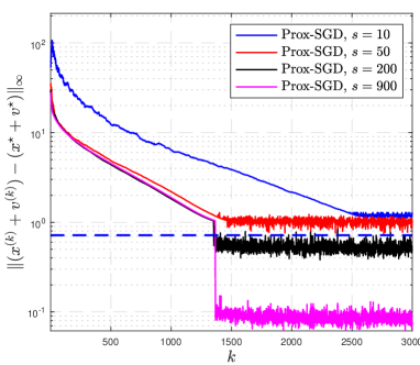
Figure 4: Error via $\ell_{\infty}$-norm.

5.2.2 Identification under degeneracy

In this part, we present a toy example to explain the identification property under degeneracy condition. Consider the following simple

$$\min_{x}\,\lambda f(x)+{{\frac{\raisebox{1.24994pt}{\small$1$}}{\raisebox{-2.08333pt}{\small$2$}}}}{|\kern-1.125pt|}x-b{|\kern-1.125pt|}^{2}$$

where $f(x)$ takes $\ell_{1}$-norm and nuclear norm. Note that solution of the problem is rather straightforward to obtain as it is computing the proximal operator of $f$. However, we can solve it with Forward–Backward splitting method [24] with small step-size to observe the degenerate behavior.

Below we discuss case by case by fixing $\lambda=1$, since the examples are only for illustrative purpose, the problems are rather small. The MATLAB variable-precision arithmetic vpa is used such that we can use high precision computation, and we use ${|\kern-1.125pt|}x^{(k)}-\bar{x}{|\kern-1.125pt|}\leq 10^{-20}$ as stopping criterion.

$\ell_{1}$-norm $f(x)={|\kern-1.125pt|}x{|\kern-1.125pt|}_{1}$

Let $b=\big{[}3,1,0.5\big{]}^{\top}$, then the solution is $\bar{x}=\big{[}2,0,0\big{]}^{\top}$. Moreover, we have the corresponding dual vector $\bar{u}$ reads

$$\bar{u}=b-\bar{x}=\big{[}1,1,0\big{]}^{\top}\in\mathrm{bdy}\big{(}{\partial{|\kern-1.125pt|}\cdot{|\kern-1.125pt|}_{1}(\bar{x})}\big{)}.$$

which violates the non-degeneracy condition at the second element as $\bar{x}_{2}=0$ while $\bar{u}_{2}=1$. Therefore, the minimal manifold and the enlarged manifold are

$$\mathcal{M}=\big{[}\mathbb{R},0,0\big{]}^{\top}\enskip\text{and}\enskip\widehat{\mathcal{M}}=\big{[}\mathbb{R},\mathbb{R},0\big{]}^{\top}.$$

respectively.

Two choices of starting point $x^{(0)}$ are considered

$$\textrm{Choice 1: $x^{(0)}=\big{[}2,2,2\big{]}^{\top}$}\qquad\text{and}\qquad\textrm{Choice 2: $x^{(0)}=\big{[}0,-2,-2\big{]}^{\top}$}.$$

For both choices, the support size of $\{x^{(k)}\}_{k\in\mathbb{N}}$ are provided in Figure 5 (a)

• For Choice 1 starting point, the sequence $\{x^{(k)}\}_{k\in\mathbb{N}}$ identifies the enlarged manifold.

• For Choice 2 starting point, the sequence $\{x^{(k)}\}_{k\in\mathbb{N}}$ identifies the correct minimal manifold of $\bar{x}$.

The above difference indicates that the when the problem is degenerate, the manifold identified depends on the direction of $x^{(0)}$ relative to the solution $\bar{x}$.

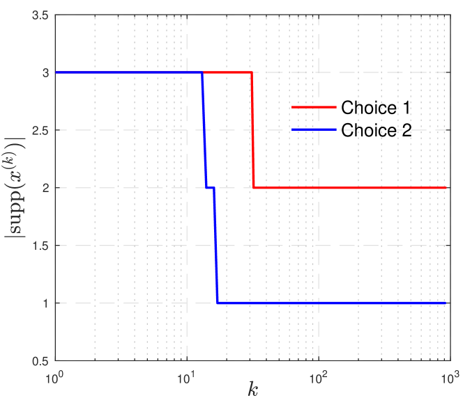
(a) Support size of $x^{(k)}$

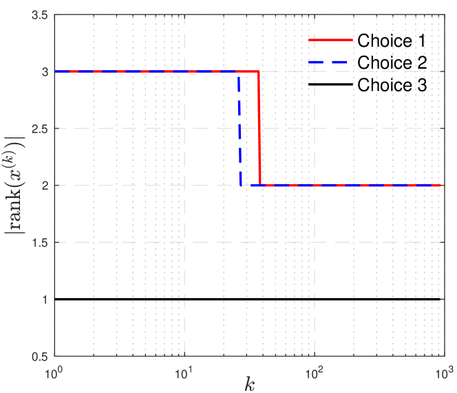
(b) Rank size of $x^{(k)}$

Figure 5: Manifold identification of $\ell_{1}$-norm and nuclear norm under degenerate condition.

Nuclear norm $f(x)={|\kern-1.125pt|}x{|\kern-1.125pt|}_{*}$

Let $b\in\mathbb{R}^{3\times 3}$ with singular value decomposition (SVD) as $[u,s,v]={\tt svd}(b)$ with $s=\mathrm{diag}\big{(}{[3,1,0.5]}\big{)}$. With $\lambda=1$, the singular value of $\bar{x}$ is $\big{[}2,0,0\big{]}$. Correspondingly, the dual vector $\bar{u}$ reads

$$\bar{u}=b-\bar{x}=u\ \mathrm{diag}\big{(}{[1,1,0\big{]}}\big{)}\ v^{\top}\in\mathrm{bdy}\big{(}{\partial{|\kern-1.125pt|}\cdot{|\kern-1.125pt|}_{*}(\bar{x})}\big{)}.$$

which violates the non-degeneracy condition at the second singular value. Therefore, the minimal manifold and the enlarged manifold are

$$\mathcal{M}=\big{\{}x\in\mathbb{R}^{3\times 3}\mid\mathrm{rank}(x)=1\big{\}}\enskip\text{and}\enskip\widehat{\mathcal{M}}=\big{\{}x\in\mathbb{R}^{3\times 3}\mid\mathrm{rank}(x)=2\big{\}}.$$

respectively.

Two choices of starting point $x^{(0)}$ are considered

$$\textrm{Choice 1: $x^{(0)}=u\ \mathrm{diag}\big{(}{[3,3,3\big{]}}\big{)}\ v^{\top}$},\quad\textrm{Choice 2: $x^{(0)}={\tt randn}(3,3)$}\,\enskip\text{and}\enskip\,\textrm{Choice 3: $x^{(0)}=0$}.$$

For all choices, the rank of $\{x^{(k)}\}_{k\in\mathbb{N}}$ are provided in Figure 5 (b), in this experiment, we treat values smaller than $10^{-30}$ as zero

• For Choice 1 & 2 starting points, the sequence $\{x^{(k)}\}_{k\in\mathbb{N}}$ identifies the enlarged manifold.

• For Choice 3 starting point, the sequence $\{x^{(k)}\}_{k\in\mathbb{N}}$ identifies the correct minimal manifold of $\bar{x}$.

Compared to $\ell_{1}$-norm case, since the singular values are non-negative and the direction is encoded in the eigenvectors, we found that $x^{(k)}$ always identifies the enlarged manifold as long as $x^{(0)}\neq 0$.

5.2.3 Upper bound of number of steps for identification

To conclude this section, we illustrate the estimation of the identification step with the following optimization problem

$$\min_{x}{{\frac{\raisebox{1.24994pt}{\small$1$}}{\raisebox{-2.08333pt}{\small$2$}}}}{|\kern-1.125pt|}Ax-b{|\kern-1.125pt|}_{2}^{2}+\lambda{|\kern-1.125pt|}x{|\kern-1.125pt|}_{1}+{{\frac{\raisebox{1.24994pt}{\small$\alpha$}}{\raisebox{-2.08333pt}{\small$2$}}}}{|\kern-1.125pt|}x{|\kern-1.125pt|}_{2}^{2},$$ (5.10)

where $A\in\mathbb{R}^{m\times n}$, $\lambda,\ \alpha>0$. The term $\frac{\alpha}{2}{|\kern-1.125pt|}x{|\kern-1.125pt|}_{2}^{2}$ is introduced to ensure strong convexity of the objective function such that Forward-Backward splitting method enjoys global linear convergence for both $\{x^{(k)}\}_{k\in\mathbb{N}}$ and $\{u^{(k)}\}_{k\in\mathbb{N}}$.

Based on Proposition 4.15 and Example 4.17, we can derive an upper bound for the identification step. To validate this, we consider a problem with dimensions $(m,n)=(20,32)$ and run the method with stopping criterion ${|\kern-1.125pt|}x^{(k)}-x^{(k-1)}{|\kern-1.125pt|}<10^{-15}$. Figure 6 illustrates the evolution of the support of $x^{(k)}$ over iterations. The location of the red dashed line is our estimation of the number of steps for identification. Note that our upper bound is quite loose which is the consequence of the inequalities involved in the derivation. Nonetheless, the experiments validates our result in Proposition 4.15.

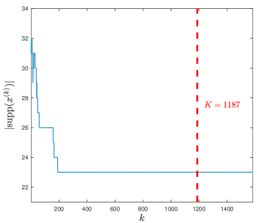
Figure 6: Identification of $x^{(k)}$ and the estimated identification step. The red dashed line represents the upper bound for the number of steps required for identification.

6 Conclusion

In this paper, we proposed the definition of partly smooth operators as a complement to [14], offering a new perspective on partial smoothness with a geometric explanation. Under the framework of partial smoothness, we demonstrated the identification property under more relaxed conditions, specifically for non-convergent dual sequences and no degenerate assumptions. We conducted numerical experiments to illustrate our theory, showing that identification can occur even when the dual vector is not convergent. For instance, in the mini-batch stochastic gradient descent (SGD) example, identification still takes place when the batch size is sufficiently large, indicating that the bounded distance of dual vector is enough to promise identification. Furthermore, under the local union structure, we revealed additional noteworthy results, including an estimation of the upper bound for the identification step. While this has been mentioned in the literature such as [17, 16]. As long as the operator exhibits local smoothness and the algorithm satisfies the appropriate properties, we can derive a suitable estimation.

Acknowledgements

JL is supported by the “Fundamental Research Funds for the Central Universities”, the National Science Foundation of China (BC4190065) and the Shanghai Municipal Science and Technology Major Project (2021SHZDZX0102).

References

- [1] J.-P. Aubin and H. Frankowska. Set-valued analysis. Springer Science & Business Media, 2009.
- [2] J. B. Baillon and G. Haddad. Quelques propriétés des opérateurs angle-bornés etn-cycliquement monotones. Israel Journal of Mathematics, 26(2):137–150, 1977.
- [3] H. Bauschke and P. L. Combettes. Convex Analysis and Monotone Operator Theory in Hilbert Spaces. Springer, 2011.
- [4] A. Chambolle and T. Pock. A first-order Primal–Dual algorithm for convex problems with applications to imaging. Journal of Mathematical Imaging and Vision, 40(1):120–145, 2011.
- [5] P. L. Combettes and J. C. Pesquet. Primal–Dual splitting algorithm for solving inclusions with mixtures of composite, Lipschitzian, and parallel-sum type monotone operators. Set-Valued and variational analysis, 20(2):307–330, 2012.
- [6] D. Drusvyatskiy and A. S. Lewis. Optimality, identifiability, and sensitivity. Mathematical Programming, 147(1-2):467–498, 2014.
- [7] Dmitriy Drusvyatskiy and Adrian S Lewis. Tilt stability, uniform quadratic growth, and strong metric regularity of the subdifferential. SIAM Journal on Optimization, 23(1):256–267, 2013.
- [8] J. Fadili, J. Malick, and G. Peyré. Sensitivity analysis for mirror-stratifiable convex functions. SIAM Journal on Optimization, 28(4):2975–3000, 2018.
- [9] Jalal Fadili, Jérôme Malick, and Gabriel Peyré. Sensitivity analysis for mirror-stratifiable convex functions. SIAM Journal on Optimization, 28(4):2975–3000, 2018.
- [10] W. L. Hare and A. S. Lewis. Identifying active constraints via partial smoothness and prox-regularity. Journal of Convex Analysis, 11(2):251–266, 2004.
- [11] Claude Lemaréchal, François Oustry, and Claudia Sagastizábal. The -lagrangian of a convex function. Transactions of the American mathematical Society, 352(2):711–729, 2000.
- [12] A. S. Lewis. Active sets, nonsmoothness, and sensitivity. SIAM Journal on Optimization, 13(3):702–725, 2003.
- [13] A. S. Lewis and S. Zhang. Partial smoothness, tilt stability, and generalized hessians. SIAM Journal on Optimization, 23(1):74–94, 2013.
- [14] Adrian S. Lewis, Jingwei Liang, and Tonghua Tian. Partial smoothness and constant rank. SIAM Journal on Optimization, 32(1):276–291, 2022.
- [15] J. Liang, J. Fadili, and G. Peyré. Local linear convergence of forward–backward under partial smoothness. In Advances in Neural Information Processing Systems, pages 1970–1978, 2014.
- [16] J. Liang, M. J. Fadili, and G. Peyré. Convergence rates with inexact nonexpansive operators. arXiv preprint arXiv:1404.4837, 2014.
- [17] J. Liang, M. J. Fadili, and G. Peyré. Activity identification and local linear convergence of Forward–Backward-type methods. arXiv:1503.03703, 2015.
- [18] Jingwei Liang. Convergence rates of first-order operator splitting methods. PhD thesis, Normandie Université; GREYC CNRS UMR 6072, 2016.
- [19] Jingwei Liang, Jalal Fadili, and Gabriel Peyré. Convergence rates with inexact non-expansive operators. Mathematical Programming, 159(1):403–434, 2016.
- [20] Jingwei Liang, Jalal Fadili, and Gabriel Peyré. Activity identification and local linear convergence of forward–backward-type methods. SIAM Journal on Optimization, 27(1):408–437, 2017.
- [21] Jingwei Liang, Jalal Fadili, and Gabriel Peyré. Local convergence properties of douglas–rachford and alternating direction method of multipliers. Journal of Optimization Theory and Applications, 172:874–913, 2017.
- [22] Jingwei Liang, Jalal Fadili, and Gabriel Peyré. Local linear convergence analysis of primal–dual splitting methods. Optimization, 67(6):821–853, Jun 2018.
- [23] Jingwei Liang, Tao Luo, and Carola-Bibiane Schönlieb. Improving “fast iterative shrinkage-thresholding algorithm”: Faster, smarter, and greedier. SIAM Journal on Scientific Computing, 44(3):A1069–A1091, 2022.
- [24] P. L. Lions and B. Mercier. Splitting algorithms for the sum of two nonlinear operators. SIAM Journal on Numerical Analysis, 16(6):964–979, 1979.
- [25] Robert Mifflin and Claudia Sagastizábal. -smoothness and proximal point results for some nonconvex functions. Optimization Methods and Software, 19(5):463–478, 2004.
- [26] B.S. Mordukhovich. Sensitivity analysis in nonsmooth optimization. Theoretical Aspects of Industrial Design (D. A. Field and V. Komkov, eds.), SIAM Volumes in Applied Mathematics, 58:32–46, 1992.
- [27] R. Poliquin and R. T. Rockafellar. Prox-regular functions in variational analysis. Transactions of the American Mathematical Society, 348(5):1805–1838, 1996.
- [28] Clarice Poon and Jingwei Liang. Trajectory of alternating direction method of multipliers and adaptive acceleration. Advances in neural information processing systems, 32, 2019.
- [29] Clarice Poon Poon, Jingwei Liang, and Carola-Bibiane Schönlieb. Local convergence properties of SAGA/Prox-SVRG and acceleration. In ICML, ICML.
- [30] Herbert Robbins and Sutton Monro. A stochastic approximation method. The Annals of Mathematical Statistics, 22(3):400–407, 1951.
- [31] R. T. Rockafellar and R. Wets. Variational analysis, volume 317. Springer Verlag, 1998.
- [32] Y Sun, H Jeong, J Nutini, and M Schmidt. Are we there yet? manifold identification of gradient-related proximal methods. In The 22nd International Conference on Artificial Intelligence and Statistics, pages 1110–1119. PMLR, 2019.
- [33] S. Vaiter, G. Peyré, and J. M. Fadili. Model consistency of partly smooth regularizers. Preprint, 2014.
- [34] S. J. Wright. Identifiable surfaces in constrained optimization. SIAM Journal on Control and Optimization, 31(4):1063–1079, 1993.