Systematic analysis of the form factors of $B_{c}$ to $P$-wave charmonia and corresponding weak decays

Abstract

In this article, the vector, axial vector and tensor form factors of $B_{c}\to\chi_{cJ}$ ($J=0,1,2$) and $B_{c}\to h_{c}$ are analyzed within the framework of three-point QCD sum rules. With the calculated vector and axial vector form factors, we directly study the decay widths and branching ratios of semileptonic decays $B_{c}^{-}\to\chi_{cJ}l\bar{\nu}_{l},h_{c}l\bar{\nu}_{l}$ $(l=e,\mu$ and $\tau)$ and analyze the nonleptonic decays $B_{c}^{-}\to\chi_{cJ}\pi^{-},\chi_{cJ}K^{-},\chi_{cJ}\rho^{-},\chi_{cJ}K^{*-}$, $B_{c}^{-}\to h_{c}\pi^{-},h_{c}K^{-},h_{c}\rho^{-},h_{c}K^{*-}$ by using the naive factorization approach (NFA). These results can provide more information to understand the properties of $B_{c}$ meson and $P$-wave charmonia and to study the heavy quark dynamics.

I Introduction

Since the $B_{c}$ meson was firstly observed by CDF collaboration in 1998 Abe et al. (1998), most of theoretical and experimental physicists payed much attention to it for the special properties. Firstly, as the only quarkonium with mixed heavy flavor quarks, $B_{c}$ meson has rich decay channels because each heavy quark in it can decay individually and the other acts as a spectator. Secondly, the mass of $B_{c}$ meson lies below the threshold of $B\bar{D}$, thus the $B_{c}$ meson can only decay via weak interaction. This provides a suitable place to test the standard model (SM) and find the new physics beyond the SM. Thirdly, both $b$ and $c$ quarks can annihilate and provide new kinds of weak decays with sizable partial decay widths. These pure leptonic or radiative leptonic decay can be used to extract the decay constant of $B_{c}$ and the Cabibbo-Kobayashi-Maskawa (CKM) matrix element $V_{cb}$ Chang and Chen (1994); Chang et al. (1998). In addition, the $B_{c}$ meson includes two different heavy flavor quarks, the spectroscopy may be different with the light mesons or the mesons with only one heavy quark. It offers us a different laboratory to study the strong interactions. Moreover, it was estimated that the inclusive production cross sections of $B_{c}$ meson and its resonance states at the LHC is at level of 1 $\mathrm{\mu b}$ for $\sqrt{14}$ TeV. This means that there are about $O(10^{9})$ $B_{c}$ meson can be anticipated in 1 fb^-1 Gao et al. (2010). So, abundant events in experiment can provide more information to carry out this research.

The weak decays of $B_{c}$ to charmonia including semileptonic and nonleptonic processes are interesting and valuable. Taking $B_{c}^{-}$ meson as an example, its weak decay processes can be described as $b$ quark decaying while the other $\bar{c}$ quark playing as a spectator at the quark level. In the case of semileptonic decays, the decay mode of $b$ quark is $b\to cl\bar{\nu}_{l}$ ($l=e,\mu$ and $\tau$). The final $c$ quark will combine with the spectator $\bar{c}$ quark to produce final charmonium. In the nonleptonic decay processes, the decay modes of $b$ quark include $b\to c\bar{u}d$, $c\bar{u}s$, $cd\bar{c}$ and $cs\bar{c}$. Except for the final $c$ quark that combines with spectator $\bar{c}$ quark to produce final charmonium, the rest quarks combine with each other to produce another final meson. Theoretical investigations about these decay processes are difficult because the quantum chromodynamics (QCD) is non-perturbative in low energy regions. Therefore, some non-perturbative methods have been employed to study the decay processes of $B_{c}$ to charmonia in recent years, such as the lattice QCD (LQCD) Colquhoun et al. (2016); Harrison et al. (2020), the QCD sum rules (QCDSR) Colangelo et al. (1993); Kiselev et al. (2000); Azizi et al. (2009, 2013); Wu et al. (2024), the light-cone QCD sum rules (LCSR) Huang and Zuo (2007); Wang and Lu (2008); Leljak et al. (2019); Bordone et al. (2023), the perturbative QCD (pQCD) Kiselev et al. (2002); Rui (2018); Liu et al. (2018, 2020), the relativistic quark model (RQM) Nobes and Woloshyn (2000); Ivanov et al. (2006); Ebert et al. (2010), the non-relativistic quark model (NRQM) Hernandez et al. (2006), the light-front quark model (LFQM) Wang et al. (2009a, b); Zhang et al. (2023); Li et al. (2023), non-relativistic QCD (NRQCD) Qiao et al. (2014); Zhu (2018); Tang et al. (2022) and other methods Chang et al. (2002); Tran et al. (2018). With the updated high luminosity of the LHC, more experimental measurements of $B_{c}$ to charmoina will become feasible in the coming years, this will provide more information to test various theoretical models.

As one of the most powerful non-perturbative approach, the QCD sum rules are widely used in studying the properties of hadrons such as the masses, decay constants and light-cone distribution amplitude of hadrons Wei et al. (2007); Wang (2013a); Chen et al. (2015); Wang (2015); Chen et al. (2016); Zhang et al. (2021); Wang (2022); Huang et al. (2023); Su et al. (2024); Wang (2024), the form factors of hadron transition Wang et al. (2008, 2009c); Shi et al. (2020); Peng and Yang (2020); Zhao et al. (2020); Neishabouri et al. (2024); Tousi et al. (2024); Lu et al. (2024), the coupling constants of strong interaction Bracco et al. (2012); Wang (2014); Azizi et al. (2014, 2015); Yu et al. (2015); Rodrigues et al. (2017); Yu et al. (2019); Lu et al. (2023a, b) and others Wang (2018); Dehghan et al. (2023); Özdem and Azizi (2024). In our previous work, the scalar, vector, axial vector and tensor form factors of $B_{c}$ to $S$-wave charmonia $\eta_{c}$ and $J/\psi$ were analyzed in the framework of three-point QCD sum rules, and the corresponding semileptonic and nonleptonic decays processes were studied Wu et al. (2024). As a continuation of our previous work, we systematically analyze the vector, axial vector and tensor form factors of $B_{c}$ to $P$-wave charmonia $\chi_{cJ}(J=0,1,2)$ and $h_{c}$ by using three-point QCD sum rules in the present work. With these form factors, we also study the semileptonic decay processes $B_{c}^{-}\to\chi_{cJ}l\bar{\nu}_{l},h_{c}l\bar{\nu}_{l}$ $(l=e,\mu$ and $\tau)$ and the nonleptonic decay processes $B_{c}^{-}\to\chi_{cJ}\pi^{-},\chi_{cJ}K^{-},\chi_{cJ}\rho^{-},\chi_{cJ}K^{*-}$, $B_{c}^{-}\to h_{c}\pi^{-},h_{c}K^{-},h_{c}\rho^{-},h_{c}K^{*-}$. The nonleptonic decay $B_{c}\to\chi_{cJ}D_{(s)}^{(*)}$ and $h_{c}D_{(s)}^{(*)}$ are also related to the form factors in this study. However, other form factors involved in these decay processes, are beyond the scope of the present work.

This work is organized as follows. After introduction, the form factors of $B_{c}$ to $P$-wave charmonia are analyzed by three-point QCD sum rules in Sec. II. Based on these form factors, we analyze the corresponding semileptonic and nonleptonic decay widths and branching ratios in Sec. III. Sec. IV is employed to present the numerical results and discussions and Sec. V is devoted to a short summary. Some important figures and formulas are shown in Appendixes A$\sim$C.

II Three-point QCD sum rules for transition form factors

To study the form factors of $B_{c}$ to $P$-wave charmonia, we firstly write down the following three-point correlation function,

$$\Pi(p,p^{\prime}) =i^{2}\int d^{4}xd^{4}ye^{ip^{\prime}x}e^{i(p-p^{\prime})y}$$ (1)

$$\times\left\langle 0\right|T\{J_{X}(x)\tilde{J}(y)J_{B_{c}}^{+}(0)\}\left|0\right\rangle$$

where $T$ denotes the time ordered product, $J_{B_{c}}$ and $J_{X}$ ($X=\chi_{cJ}$ and $h_{c}$, $J=0,1,2$) are the interpolating currents of $B_{c}$ meson and $P$-wave charmonia, respectively. $\tilde{J}$ is the transition currents. These currents are taken as following forms,

$$J_{B_{c}}(0) =\bar{c}(0)i\gamma_{5}b(0)$$

$$\tilde{J}(y) =\bar{c}(y)\Gamma b(y)$$

$$J^{\chi_{c0}}(x) =\bar{c}(x)c(x)$$

$$J_{\mu}^{\chi_{c1}}(x) =\bar{c}(x)\gamma_{\mu}\gamma_{5}c(x)$$

$$J_{\mu\nu}^{h_{c}}(x) =\bar{c}(x)\sigma_{\mu\nu}c(x)$$

$$J_{\mu\nu}^{\chi_{c2}}(x) =\frac{i}{2}\bar{c}(x)({\gamma_{\mu}}{\mathord{\buildrel{\lower 3.0pt\hbox{$\scriptscriptstyle\leftrightarrow$}}\over{D}}}_{\nu}+{\gamma_{\nu}}{{\mathord{\buildrel{\lower 3.0pt\hbox{$\scriptscriptstyle\leftrightarrow$}}\over{D}}}_{\mu}})c(x)$$ (2)

where $\Gamma=\gamma_{\mu},\gamma_{\mu}\gamma_{5}$ and $\sigma_{\mu\nu}$ or $\sigma_{\mu\nu}\gamma_{5}$ for vector, axial vector and tensor form factors, respectively. $\mathord{\buildrel{\lower 3.0pt\hbox{$\scriptscriptstyle\leftrightarrow$}}\over{D}}_{\mu}=\frac{1}{2}(\mathord{\buildrel{\lower 3.0pt\hbox{$\scriptscriptstyle\rightarrow$}}\over{D}}_{\mu}-\mathord{\buildrel{\lower 3.0pt\hbox{$\scriptscriptstyle\leftarrow$}}\over{D}}_{\mu})$, $\mathord{\buildrel{\lower 3.0pt\hbox{$\scriptscriptstyle\rightarrow$}}\over{D}}_{\mu}=\mathord{\buildrel{\lower 3.0pt\hbox{$\scriptscriptstyle\rightarrow$}}\over{\partial}}_{\mu}-ig_{s}G_{\mu}$ denote the covariant derivative.

In the framework of QCD sum rules, the correlation function will be calculated at both hadron and quark levels which are called phenomenological side and QCD side, respectively. Combining these two sides by using quark hadron duality, the sum rules for the form factors will be derived.

II.1 The phenomenological side

In phenomenological side, complete sets of hadronic states with the same quantum numbers as interpolating currents are inserted in correlation function in Eq. (1). Performing the integration in coordinate space and using the double dispersion relation, the correlation function can be written as the following form Colangelo and Khodjamirian (2000),

$$\Pi^{\mathrm{phy}}(p,p^{\prime}) =\frac{\left\langle 0\right|J_{X}(0)\left|X(p^{\prime})\right\rangle\left\langle B_{c}(p)\right|J_{B_{c}}^{+}(0)\left|0\right\rangle}{(p^{\prime 2}-m_{X}^{2})(p^{2}-m_{B_{c}}^{2})}$$ (3)

$$\times\left\langle X(p^{\prime})\right|\tilde{J}(0)\left|B_{c}(p)\right\rangle+...$$

where the ellipsis represent the contributions of higher resonances and continuum states. The meson vacuum matrix elements in above correlation function are defined as,

$$\left\langle 0\right|J^{\chi_{c0}}(0)\left|\chi_{c0}(p^{\prime})\right\rangle =f_{\chi_{c0}}m_{\chi_{c0}}$$

$$\left\langle 0\right|J_{\mu}^{\chi_{c1}}(0)\left|\chi_{c1}(p^{\prime})\right\rangle =f_{\chi_{c1}}m_{\chi_{c1}}\epsilon^{\chi_{c1}}_{\mu}$$

$$\left\langle 0\right|J_{\mu}^{\chi_{c1}}(0)\left|{\eta_{c}}(p^{\prime})\right\rangle =if_{\eta_{c}}p^{\prime}_{\mu}$$

$$\left\langle 0\right|J_{\mu\nu}^{h_{c}}(0)\left|h_{c}(p^{\prime})\right\rangle =if_{h_{c}}\varepsilon_{\mu\nu\alpha\beta}\epsilon^{h_{c}}_{\alpha}p^{\prime}_{\beta}$$

$$\left\langle 0\right|J_{\mu\nu}^{h_{c}}(0)\left|J/\psi(p^{\prime})\right\rangle =if_{J/\psi}(p^{\prime}_{\mu}\epsilon^{J/\psi}_{\nu}-p^{\prime}_{\nu}\epsilon^{J/\psi}_{\mu})$$

$$\left\langle 0\right|J_{\mu\nu}^{\chi_{c2}}(0)\left|\chi_{c2}(p^{\prime})\right\rangle =f_{\chi_{c2}}m_{\chi_{c2}}^{3}\epsilon^{\chi_{c2}}_{\mu\nu}$$

$$\left\langle B_{c}(p)\right|J_{B_{c}}^{+}(0)\left|0\right\rangle =\frac{f_{B_{c}}m_{B_{c}}^{2}}{m_{b}+m_{c}}$$ (4)

where $f_{\chi_{c0}}$, $f_{\chi_{c1}}$, $f_{\eta_{c}}$, $f_{h_{c}}$, $f_{J/\psi}$, $f_{\chi_{c2}}$ and $f_{B_{c}}$ are the decay constants of corresponding mesons, $\epsilon^{\chi_{c1}}_{\mu}$, $\epsilon^{h_{c}}_{\alpha}$ and $\epsilon^{J/\psi}_{\mu}$ are the polarization vectors of $\chi_{c1}$, $h_{c}$ and $J/\psi$, respectively. $\epsilon^{\chi_{c2}}_{\mu\nu}$ is the polarization tensor of $\chi_{c2}$, and $\varepsilon_{\mu\nu\alpha\beta}$ is the 4-dimension Levi-Civita tensor. It is noted that the current of $\chi_{c1}$ ($J^{P}=1^{+}$) can couple with the pseudoscalar charmonium $\eta_{c}$ ($J^{P}=0^{-}$). The tensor current $\bar{c}\sigma_{\mu\nu}c$ which is selected to interpolate $h_{c}$ ($J^{P}=1^{+}$) can also couple with $J/\psi$ ($J^{P}=1^{-}$). In order to eliminate the contamination of the redundant coupling, the projection operator should be induced in corresponding correlation function which will be discussed in next sections. The transition matrix elements in Eq. (3) can be expressed in terms of various form factors. For the vector and axial vector form factors, the Bauer-Stech-Wirbel (BWS) forms are more frequently used and defined as Wirbel et al. (1985),

$$\left\langle\chi_{c0}(p^{\prime})\right|\bar{c}(0)\gamma_{\mu}\gamma_{5}b(0)\left|B_{c}(p)\right\rangle=F_{0}^{{B_{c}}\to\chi_{c0}}(q^{2})\frac{m_{B_{c}}^{2}-m_{\chi_{c0}}^{2}}{q^{2}}q_{\mu}$$

$$+F_{1}^{{B_{c}}\to\chi_{c0}}(q^{2})\left(p_{\mu}+p^{\prime}_{\mu}-\frac{m_{B_{c}}^{2}-m_{\chi_{c0}}^{2}}{q^{2}}q_{\mu}\right)$$ (5)

$$\left\langle\chi_{c1}[{h_{c}}](p^{\prime})\right|\bar{c}(0)\gamma_{\mu}b(0)\left|{B_{c}}(p)\right\rangle$$

$$=-i\big{(}m_{B_{c}}-m_{\chi_{c1}[h_{c}]}\big{)}V_{1}^{B_{c}\to\chi_{c1}[h_{c}]}(q^{2})\epsilon^{\chi_{c1}[h_{c}]*}_{\mu}$$

$$+iV_{2}^{B_{c}\to\chi_{c1}[h_{c}]}(q^{2})\frac{\epsilon^{\chi_{c1}[h_{c}]*}\cdot P}{m_{B_{c}}-m_{\chi_{c1}[h_{c}]}}P_{\mu}$$

$$+2im_{\chi_{c1}[h_{c}]}\left[V_{3}^{B_{c}\to\chi_{c1}[h_{c}]}(q^{2})-V_{0}^{B_{c}\to\chi_{c1}[h_{c}]}(q^{2})\right]\frac{\epsilon^{\chi_{c1}[h_{c}]*}\cdot P}{q^{2}}q_{\mu}$$

$$\left\langle\chi_{c1}[h_{c}](p^{\prime})\right|\bar{c}(0)\gamma_{\mu}\gamma_{5}b(0)\left|B_{c}(p)\right\rangle$$

$$=-\frac{A^{B_{c}\to\chi_{c1}[h_{c}]}(q^{2})}{m_{B_{c}}-m_{\chi_{c1}[h_{c}]}}\varepsilon_{\mu\alpha\beta\gamma}\epsilon^{\chi_{c1}[h_{c}]*}_{\alpha}P_{\beta}q_{\gamma}$$ (6)

$$\left\langle\chi_{c2}(p^{\prime})\right|\bar{c}(0)\gamma_{\mu}b(0)\left|B_{c}(p)\right\rangle=h^{B_{c}\to\chi_{c2}}(q^{2})\varepsilon_{\mu\beta\rho\sigma}\epsilon^{\chi_{c2}*}_{\beta\lambda}P^{\lambda}P^{\rho}q^{\sigma}$$

$$\left\langle\chi_{c2}(p^{\prime})\right|\bar{c}(0)\gamma_{\mu}\gamma_{5}b(0)\left|B_{c}(p)\right\rangle=-i\ k^{B_{c}\to\chi_{c2}}(q^{2})\epsilon^{\chi_{c2}*}_{\mu\beta}P^{\beta}$$

$$-i\epsilon^{\chi_{c2}*}_{\beta\lambda}P^{\beta}P^{\lambda}\left[b_{+}^{B_{c}\to\chi_{c2}}(q^{2})P_{\mu}+b_{-}^{B_{c}\to\chi_{c2}}(q^{2})q_{\mu}\right]$$ (7)

where $P=p+p^{\prime}$ and $q=p-p^{\prime}$. $F_{0}$ and $F_{1}$ are axial vector form factors of $\chi_{c0}$, the vector form factors of $\chi_{c0}$ do not exist due to the conservation of angular momentum. $A$ and $V_{0}$/$V_{1}$/$V_{2}$ are axial vector and vector form factors of $\chi_{c1}$ and $h_{c}$. $V_{3}$ in Eq. (II.1) has the following form,

$$V_{3}^{B_{c}\to\chi_{c1}[h_{c}]}(q^{2}) =\frac{m_{B_{c}}-m_{\chi_{c1}[h_{c}]}}{2m_{\chi_{c1}[h_{c}]}}V_{1}^{B_{c}\to\chi_{c1}[h_{c}]}(q^{2})$$ (8)

$$-\frac{m_{B_{c}}+m_{\chi_{c1}[h_{c}]}}{2m_{\chi_{c1}[h_{c}]}}V_{2}^{B_{c}\to\chi_{c1}[h_{c}]}(q^{2})$$

$h$ and $k/b_{+}/b_{-}$ in Eq. (II.1) are vector and axial vector form factors of $B_{c}\to\chi_{c2}$. In order to simplify the calculations of scatter amplitude, the following substitutions are commonly used Wang et al. (2009b),

$$A^{B_{c}\to\chi_{c2}}(q^{2}) =-\big{(}m_{B_{c}}-m_{\chi_{c2}}\big{)}h^{B_{c}\to\chi_{c2}}(q^{2})$$

$$V_{1}^{B_{c}\to\chi_{c2}}(q^{2}) =-\frac{k^{B_{c}\to\chi_{c2}}(q^{2})}{m_{B_{c}}-m_{\chi_{c2}}}$$

$$V_{2}^{B_{c}\to\chi_{c2}}(q^{2}) =\big{(}m_{B_{c}}-m_{\chi_{c2}}\big{)}b_{+}^{B_{c}\to\chi_{c2}}(q^{2})$$

$$V_{0}^{B_{c}\to\chi_{c2}}(q^{2}) =\frac{m_{B_{c}}-m_{\chi_{c2}}}{2m_{\chi_{c2}}}V_{1}^{B_{c}\to\chi_{c2}}(q^{2})$$

$$-\frac{m_{B_{c}}+m_{\chi_{c2}}}{2m_{\chi_{c2}}}V_{2}^{B_{c}\to\chi_{c2}}(q^{2})-\frac{q^{2}}{2m_{\chi_{c2}}}b_{-}^{B_{c}\to\chi_{c2}}(q^{2})$$

The tensor form factors of $B_{c}\to\chi_{cJ}$ and $h_{c}$ are defined as follows Colangelo et al. (2022),

$$\left\langle\chi_{c0}(p^{\prime})\right|\bar{c}(0)\sigma_{\mu\nu}b(0)\left|B_{c}(p)\right\rangle=-\frac{T^{B_{c}\to\chi_{c0}}(q^{2})}{m_{B_{c}}-m_{\chi_{c0}}}\varepsilon_{\mu\nu\alpha\beta}p^{\alpha}p^{\prime\beta}$$ (10)

$$\left\langle\chi_{c1}[h_{c}](p^{\prime})\right|\bar{c}(0)\sigma_{\mu\nu}\gamma_{5}b(0)\left|B_{c}(p)\right\rangle$$

$$=-T_{0}^{B_{c}\to\chi_{c1}[h_{c}]}(q^{2})\frac{\epsilon^{\chi_{c1}[h_{c}]*}\cdot q}{\big{(}m_{B_{c}}-{m_{\chi_{c1}[h_{c}]}}\big{)}^{2}}\varepsilon_{\mu\nu\alpha\beta}p^{\alpha}p^{\prime\beta}$$

$$+T_{1}^{B_{c}\to\chi_{c1}[h_{c}]}(q^{2})\varepsilon_{\mu\nu\alpha\beta}p_{\alpha}\epsilon^{\chi_{c1}[h_{c}]*}_{\beta}$$

$$+T_{2}^{B_{c}\to\chi_{c1}[h_{c}]}(q^{2})\varepsilon_{\mu\nu\alpha\beta}p^{\prime}_{\alpha}\epsilon^{\chi_{c1}[h_{c}]*}_{\beta}$$ (11)

$$\left\langle\chi_{c2}(p^{\prime})\right|\bar{c}(0)\sigma_{\mu\nu}b(0)\left|B_{c}(p)\right\rangle$$

$$=\frac{q^{\tau}}{m_{B_{c}}}\left[T_{0}^{B_{c}\to\chi_{c2}}(q^{2})\frac{\epsilon^{\chi_{c2}*}_{\rho\tau}q^{\rho}}{\big{(}m_{B_{c}}-m_{\chi_{c2}}\big{)}^{2}}\varepsilon_{\mu\nu\chi\delta}p^{\chi}p^{\prime\delta}\right.$$

$$\left.+T_{1}^{B_{c}\to\chi_{c2}}(q^{2})\varepsilon_{\mu\nu\chi\delta}\epsilon^{\chi_{c2}*}_{\chi\tau}p_{\delta}+T_{2}^{B_{c}\to\chi_{c2}}(q^{2})\varepsilon_{\mu\nu\chi\delta}\epsilon^{\chi_{c2}*}_{\chi\tau}p^{\prime}_{\delta}\right]$$

where $T$ and $T_{0}/T_{1}/T_{2}$ are tensor form factors of $\chi_{c0}$ and $\chi_{c1}/\chi_{c2}/h_{c}$.

From these above equations, the correlation functions in phenomenological side can be obtained and be expanded into different tensor structures. In principle, each structure can be used to carry out the calculations of form factors and will lead to same results. However, the final results obtained by different structures have different uncertainties because of the truncation of operator product expansion (OPE) in QCD side and different contributions of higher resonances and continuum states Bracco et al. (1999). In this article, we will adopt the traditional way to choose the appropriate structure, where the pole contributions should be large than 50% and the stability of Borel window should be satisfied. The details will discussed in next sections.

II.2 The QCD side

In QCD side, we perform the operator product expansion (OPE) of correlation function by contracting all of the quark fields operator with Wick’s theorem. After this step, the correlation functions of all processes in QCD side are expressed as follows,

$$\Pi_{\mu}^{\chi_{c0}QCD}(p,p^{\prime}) =-i\int d^{4}xd^{4}ye^{ip^{\prime}x}e^{i(p-p^{\prime})y}$$

$$\times Tr\big{[}C^{km}(-x)C^{mn}(x-y)\gamma_{\mu}\gamma_{5}B^{nk}(y)\gamma_{5}\big{]}$$

$$\Pi_{\mu\nu}^{\chi_{c0}QCD}(p,p^{\prime}) =-i\int d^{4}xd^{4}ye^{ip^{\prime}x}e^{i(p-p^{\prime})y}$$ (13)

$$\times Tr\big{[}C^{km}(-x)C^{mn}(x-y)\sigma_{\mu\nu}B^{nk}(y)\gamma_{5}\big{]}$$

$$\Pi_{1\mu\nu}^{\chi_{c1}QCD}(p,p^{\prime}) =-i\int d^{4}xd^{4}ye^{ip^{\prime}x}e^{i(p-p^{\prime})y}$$

$$\times Tr[C^{km}(-x)\gamma_{\mu}\gamma_{5}C^{mn}(x-y)\gamma_{\nu}B^{nk}(y)\gamma_{5}]$$

$$\Pi_{2\mu\nu}^{\chi_{c1}QCD}(p,p^{\prime}) =-i\int d^{4}xd^{4}ye^{ip^{\prime}x}e^{i(p-p^{\prime})y}$$

$$\times Tr\big{[}C^{km}(-x)\gamma_{\mu}\gamma_{5}C^{mn}(x-y)\gamma_{\nu}\gamma_{5}B^{nk}(y)\gamma_{5}\big{]}$$

$$\Pi_{\mu\nu\sigma}^{\chi_{c1}QCD}(p,p^{\prime}) =-i\int d^{4}xd^{4}ye^{ip^{\prime}x}e^{i(p-p^{\prime})y}$$

$$\times Tr\big{[}C^{km}(-x)\gamma_{\mu}\gamma_{5}C^{mn}(x-y)\sigma_{\nu\sigma}\gamma_{5}B^{nk}(y)\gamma_{5}\big{]}$$

$$\Pi_{1\mu\nu\sigma}^{h_{c}QCD}(p,p^{\prime}) =-i\int d^{4}xd^{4}ye^{ip^{\prime}x}e^{i(p-p^{\prime})y}$$

$$\times Tr\big{[}C^{km}(-x)\sigma_{\mu\nu}C^{mn}(x-y)\gamma_{\sigma}B^{nk}(y)\gamma_{5}\big{]}$$

$$\Pi_{2\mu\nu\sigma}^{h_{c}QCD}(p,p^{\prime}) =-i\int d^{4}xd^{4}ye^{ip^{\prime}x}e^{i(p-p^{\prime})y}$$

$$\times Tr\big{[}C^{km}(-x)\sigma_{\mu\nu}C^{mn}(x-y)\gamma_{\sigma}\gamma_{5}B^{nk}(y)\gamma_{5}\big{]}$$

$$\Pi_{\mu\nu\alpha\beta}^{h_{c}QCD}(p,p^{\prime}) =-i\int d^{4}xd^{4}ye^{ip^{\prime}x}e^{i(p-p^{\prime})y}$$

$$\times Tr\big{[}C^{km}(-x)\sigma_{\mu\nu}C^{mn}(x-y)\sigma_{\alpha\beta}\gamma_{5}B^{nk}(y)\gamma_{5}\big{]}$$

$$\Pi_{1\mu\nu\sigma}^{\chi_{c2}QCD}(p,p^{\prime}) =\int d^{4}xd^{4}ye^{ip^{\prime}x}e^{i(p-p^{\prime})y}$$

$$\times Tr\big{[}C^{km}(-x)\Gamma_{\mu\nu}C^{mn}(x-y)\gamma_{\sigma}B^{nk}(y)\gamma_{5}\big{]}$$

$$\Pi_{2\mu\nu\sigma}^{\chi_{c2}QCD}(p,p^{\prime}) =\int d^{4}xd^{4}ye^{ip^{\prime}x}e^{i(p-p^{\prime})y}$$

$$\times Tr\big{[}C^{km}(-x)\Gamma_{\mu\nu}C^{mn}(x-y)\gamma_{\sigma}\gamma_{5}B^{nk}(y)\gamma_{5}\big{]}$$

$$\Pi_{\mu\nu\alpha\beta}^{\chi_{c2}QCD}(p,p^{\prime}) =\int d^{4}xd^{4}ye^{ip^{\prime}x}e^{i(p-p^{\prime})y}$$

$$\times Tr\big{[}C^{km}(-x)\Gamma_{\mu\nu}C^{mn}(x-y)\sigma_{\alpha\beta}B^{nk}(y)\gamma_{5}\big{]}$$

where $\Gamma_{\mu\nu}=\frac{1}{2}(\gamma_{\mu}\mathord{\buildrel{\lower 3.0pt\hbox{$\scriptscriptstyle\leftrightarrow$}}\over{D}}_{\nu}+\gamma_{\nu}\mathord{\buildrel{\lower 3.0pt\hbox{$\scriptscriptstyle\leftrightarrow$}}\over{D}}_{\mu})$, $C^{ij}(x)$ and $B^{ij}(x)$ are the full propagator of $c$ and $b$ quarks, and they can uniformly be represented as the following forms Wang and Di (2014),

$$Q^{ij}(x) =\frac{i}{(2\pi)^{4}}\int d^{4}ke^{-ik\cdot x}\left\{\frac{\delta^{ij}}{\not{k}-{m_{Q}}}\right.$$

$$-\frac{g_{s}G_{\alpha\beta}^{n}t_{ij}^{n}}{4}\frac{\sigma^{\alpha\beta}(\not{k}+{m_{Q}})+(\not{k}+{m_{Q}})\sigma^{\alpha\beta}}{(k^{2}-m_{Q}^{2})^{2}}$$

$$\left.-\frac{g_{s}^{2}({t^{a}}{t^{b}})_{ij}G_{\alpha\beta}^{a}G_{\mu\nu}^{b}(f^{\alpha\beta\mu\nu}+f^{\alpha\mu\beta\nu}+f^{\alpha\mu\nu\beta})}{4(k^{2}-m_{Q}^{2})^{5}}+...\right\}$$

Here, $Q$ denotes $C$ or $B$, $t^{n}=\frac{\lambda^{n}}{2}$, $\lambda^{n}(n=1,...,8)$ are the Gell-Mann matrices, $i$ and $j$ are color indices, $\sigma_{\alpha\beta}=\frac{i}{2}[\gamma_{\alpha},\gamma_{\beta}]$, and $f^{\alpha\beta\mu\nu}$ have the following form,

$$f^{\alpha\beta\mu\nu} =(\not{k}+m_{Q})\gamma^{\alpha}(\not{k}+m_{Q})\gamma^{\beta}(\not{k}+m_{Q})$$ (18)

$$\times\gamma^{\mu}(\not{k}+m_{Q})\gamma^{\nu}(\not{k}+m_{Q})$$

Substituting with the full propagator in Eqs. (II.2)$\sim$(II.2), the correlation functions in QCD side can also be expanded in different tensor structures,

$$\Pi_{\mu}^{\chi_{c0}QCD}(p,p^{\prime}) =\Pi_{1}^{\chi_{c0}QCD}p_{\mu}+\Pi_{2}^{\chi_{c0}QCD}p^{\prime}_{\mu}$$

$$\Pi_{\mu\nu}^{\chi_{c0}QCD}(p,p^{\prime}) =\Pi_{3}^{\chi_{c0}QCD}\varepsilon_{\mu\nu\alpha\beta}p^{\alpha}p^{\prime\beta}$$ (19)

$$\tilde{\Pi}_{1\lambda\nu}^{\chi_{c1}QCD}(p,p^{\prime}) =\big{(}g_{\lambda\mu}-\frac{p^{\prime}_{\lambda}p^{\prime}_{\mu}}{p^{\prime 2}}\big{)}\Pi_{1\mu\nu}^{\chi_{c1}QCD}(p,p^{\prime})$$

$$=\Pi_{1}^{\chi_{c1}QCD}g_{\lambda\nu}+\Pi_{2}^{\chi_{c1}QCD}p_{\lambda}p_{\nu}$$

$$+\Pi_{3}^{\chi_{c1}QCD}p_{\lambda}p^{\prime}_{\nu}+...$$

$$\tilde{\Pi}_{2\lambda\nu}^{\chi_{c1}QCD}(p,p^{\prime}) =\big{(}g_{\lambda\mu}-\frac{p^{\prime}_{\lambda}p^{\prime}_{\mu}}{p^{\prime 2}}\big{)}\Pi_{2\mu\nu}^{\chi_{c1}QCD}(p,p^{\prime})$$

$$=\Pi_{4}^{\chi_{c1}QCD}\varepsilon_{\lambda\nu\alpha\beta}p^{\alpha}p^{\prime\beta}$$

$$\tilde{\Pi}_{\lambda\nu\sigma}^{\chi_{c1}QCD}(p,p^{\prime}) =\big{(}g_{\lambda\mu}-\frac{p^{\prime}_{\lambda}p^{\prime}_{\mu}}{p^{\prime 2}}\big{)}\Pi_{\mu\nu\sigma}^{\chi_{c1}QCD}(p,p^{\prime})$$ (20)

$$=\Pi_{5}^{\chi_{c1}QCD}\varepsilon_{\lambda\nu\sigma\alpha}p^{\alpha}+\Pi_{6}^{\chi_{c1}QCD}\varepsilon_{\lambda\nu\sigma\alpha}p^{\prime\alpha}$$

$$+\Pi_{7}^{\chi_{c1}QCD}p_{\lambda}\varepsilon_{\nu\sigma\alpha\beta}p^{\alpha}p^{\prime\beta}+...$$

$$\tilde{\Pi}_{1\lambda\chi\sigma}^{h_{c}QCD}(p,p^{\prime}) =\big{(}g_{\lambda\mu}-\frac{p^{\prime}_{\lambda}p^{\prime}_{\mu}}{p^{\prime 2}}\big{)}\big{(}g_{\chi\nu}-\frac{p^{\prime}_{\chi}p^{\prime}_{\nu}}{p^{\prime 2}}\big{)}\Pi_{1\mu\nu\sigma}^{h_{c}QCD}(p,p^{\prime})$$

$$=\Pi_{1}^{h_{c}QCD}\varepsilon_{\lambda\sigma\chi\alpha}p^{\alpha}+\Pi_{2}^{h_{c}QCD}p_{\sigma}\varepsilon_{\lambda\chi\alpha\beta}p^{\alpha}p^{\prime\beta}$$

$$+\Pi_{3}^{h_{c}QCD}p^{\prime}_{\sigma}\varepsilon_{\lambda\chi\alpha\beta}p^{\alpha}p^{\prime\beta}+...$$

$$\tilde{\Pi}_{2\lambda\chi\sigma}^{h_{c}QCD}(p,p^{\prime}) =\big{(}g_{\lambda\mu}-\frac{p^{\prime}_{\lambda}p^{\prime}_{\mu}}{p^{\prime 2}}\big{)}\big{(}g_{\chi\nu}-\frac{p^{\prime}_{\chi}p^{\prime}_{\nu}}{p^{\prime 2}}\big{)}\Pi_{2\mu\nu\sigma}^{h_{c}QCD}(p,p^{\prime})$$

$$=\Pi_{4}^{h_{c}QCD}p_{\lambda}g_{\sigma\chi}+...$$

$$\bar{\Pi}_{\alpha\chi}^{h_{c}QCD}(p,p^{\prime}) =g^{\lambda\beta}\big{(}g_{\lambda\mu}-\frac{p^{\prime}_{\lambda}p^{\prime}_{\mu}}{p^{\prime 2}}\big{)}\big{(}g_{\chi\nu}-\frac{p^{\prime}_{\chi}p^{\prime}_{\nu}}{p^{\prime 2}}\big{)}\Pi_{\mu\nu\alpha\beta}^{h_{c}QCD}(p,p^{\prime})$$ (21)

$$=\Pi_{5}^{h_{c}QCD}g_{\alpha\chi}+\Pi_{6}^{h_{c}QCD}p_{\alpha}p_{\chi}$$

$$+\Pi_{7}^{h_{c}QCD}p^{\prime}_{\alpha}p_{\chi}+...$$

$$\Pi_{1\mu\nu\sigma}^{\chi_{c2}QCD}(p,p^{\prime}) =\Pi_{1}^{\chi_{c2}QCD}p_{\mu}\varepsilon_{\sigma\nu\alpha\beta}p^{\alpha}p^{\prime\beta}$$

$$\Pi_{2\mu\nu\sigma}^{\chi_{c2}QCD}(p,p^{\prime}) =\Pi_{2}^{\chi_{c2}QCD}p_{\mu}g_{\nu\sigma}+\Pi_{3}^{\chi_{c2}QCD}p_{\mu}p_{\nu}p_{\sigma}$$

$$+\Pi_{4}^{\chi_{c2}QCD}p^{\prime}_{\mu}p^{\prime}_{\nu}p^{\prime}_{\sigma}$$

$$\Pi_{\mu\nu\alpha\beta}^{\chi_{c2}QCD}(p,p^{\prime}) =\Pi_{5}^{\chi_{c2}QCD}g_{\mu\nu}\varepsilon_{\alpha\beta\chi\lambda}p^{\chi}p^{\prime\lambda}+\Pi_{6}^{\chi_{c2}QCD}p_{\mu}\varepsilon_{\nu\alpha\beta\lambda}p^{\lambda}$$ (22)

$$+\Pi_{7}^{\chi_{c2}QCD}p_{\mu}\varepsilon_{\nu\alpha\beta\lambda}p^{\prime\lambda}+...$$

The projection operator $\big{(}g_{\lambda\mu}-\frac{p^{\prime}_{\lambda}p^{\prime}_{\mu}}{p^{\prime 2}}\big{)}$ in Eq. (II.2) is introduced to eliminate the coupling of axial vector current $\bar{c}\gamma_{\mu}\gamma_{5}c$ with pseudoscalar charmonium $\eta_{c}$, and $\big{(}g_{\lambda\mu}-\frac{p^{\prime}_{\lambda}p^{\prime}_{\mu}}{p^{\prime 2}}\big{)}\big{(}g_{\chi\nu}-\frac{p^{\prime}_{\chi}p^{\prime}_{\nu}}{p^{\prime 2}}\big{)}$ in Eq. (II.2) is to eliminate the coupling of tensor current $\bar{c}\sigma_{\mu\nu}c$ with vector charmonium $J/\psi$. $\Pi^{QCD}_{i}$ in the right side of above equations are named as the scalar invariant amplitude, and can be divided into perturbative and non-perturbative parts,

$$\Pi_{i}^{QCD}(p,p^{\prime}) =\Pi^{pert}_{i}(p,p^{\prime})+\Pi^{non-pert}_{i}(p,p^{\prime})$$ (23)

where the non-perturbative part include the two gluons condensate $\langle g_{s}^{2}GG\rangle$, three gluons condensate $g_{s}^{3}\langle fGGG\rangle$, and higher dimensions condensate terms. In our previous work Wu et al. (2024); Lu et al. (2024), the contribution of three gluon condensate is small, about one-tenth that of two-gluon condensate. The higher dimension terms such as the four gluon condensate are very small and further suppressed by $O(\alpha_{s}^{2})$ $(\alpha_{s}=g_{s}^{2}/4\pi)$, so can be safely neglected in our calculations. Thus, we only reserve the two gluon condensate term as the non-perturbative contribution in our calculations. The scalar invariant amplitude can be written as the following form according to the double dispersion relation,

$$\Pi_{i}^{QCD}(p,p^{\prime}) =\int\limits_{s_{1}}^{\infty}ds\int\limits_{u_{1}}^{\infty}du\frac{\rho_{i}^{QCD}(s,u,q^{2})}{(s-p^{2})(u-p^{\prime 2})}$$ (24)

where $\rho^{QCD}(s,u,q^{2})$ is the QCD spectral density and can be expressed as,

$$\rho_{i}^{QCD}(s,u,q^{2}) =\rho^{pert}(s,u,q^{2})+\rho^{\left\langle g_{s}^{2}GG\right\rangle}(s,u,q^{2})$$ (25)

with $s=p^{2}$, $u=p^{\prime 2}$ and $q=p-p^{\prime}$. $s_{1}$ and $u_{1}$ in Eq. (24) are the kinematic limits for $B_{c}$ meson and P-wave charmonium, and they are taken as $(m_{b}+m_{c})^{2}$ and $4m_{c}^{2}$, respectively.

The QCD spectral density of the perturbative part and two gluon condensate can be obtained by using the Cutkoskys’s rules Wang et al. (2008); Shi et al. (2020), the calculation details can be found in Ref.  Wu et al. (2024). The corresponding Feynman diagrams are shown in Fig. 1.

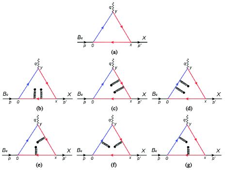
Figure 1: The Feynman diagrams for the perturbative part (a) and gluon condensate (b)$\sim$(g), where the blue and red solid lines denote the $b$ and $c$ quark lines, respectively. The black loop lines are the gluon lines.

We take the change of variables $p^{2}\to-P^{2}$, $p^{\prime 2}\to-P^{\prime 2}$ and $q^{2}\to-Q^{2}$ and perform double Borel transforms Ioffe and Smilga (1983) for the variables $P^{2}$ and $P^{\prime 2}$ to both phenomenological and QCD sides. The variables $P^{2}$ and $P^{\prime 2}$ will be replaced by Borel parameters $T_{1}^{2}$ and $T_{2}^{2}$, respectively. Then, we use the relations $T^{2}=T_{1}^{2}$ and $T_{2}^{2}=kT_{1}^{2}=kT^{2}$ to reduce the two Borel parameters, where $k=m_{X}^{2}/m_{B_{c}}^{2}$ Bracco et al. (2012), $X$ denote the P-wave charmonium. After matching the phenomenological and QCD sides by using quark-hadron duality condition, the QCD sum rules for the form factors will be obtained. Taking the axial vector form factors for $B_{c}\to\chi_{c0}$ as an example, these form factors can be obtained by combining two invariant amplitudes $\Pi^{\chi_{c0}QCD}_{1}$ and $\Pi^{\chi_{c0}QCD}_{2}$ in Eq. (II.2), and have the following forms,

$$F_{0}(Q^{2}) =-\frac{1}{2\mathcal{X}\mathcal{Y}}e^{\frac{m_{B_{c}}^{2}}{T^{2}}+\frac{m_{X}^{2}}{kT^{2}}}$$

$$\times\int\limits_{s_{1}}^{s_{0}}\int\limits_{u_{1}}^{u_{0}}dsdu\big{[}\big{(}\mathcal{X}+1)\rho_{1}^{{\chi_{c0}}QCD}(s,u,{Q^{2}}\big{)}$$

$$+\big{(}\mathcal{X}-1\big{)}\rho_{2}^{\chi_{c0}QCD}(s,u,Q^{2})\big{]}e^{-\frac{s}{T^{2}}-\frac{u}{kT^{2}}}$$

$$F_{1}(Q^{2}) =-\frac{1}{2\mathcal{Y}}e^{\frac{m_{B_{c}}^{2}}{T^{2}}+\frac{m_{X}^{2}}{kT^{2}}}$$ (26)

$$\times\int\limits_{s_{1}}^{s_{0}}\int\limits_{u_{1}}^{u_{0}}dsdu\big{[}\rho_{1}^{\chi_{c0}QCD}(s,u,Q^{2})$$

$$+\rho_{2}^{\chi_{c0}QCD}(s,u,Q^{2})\big{]}e^{-\frac{s}{T^{2}}-\frac{u}{kT^{2}}}$$

where,

$$\mathcal{X} =-\frac{m_{B_{c}}^{2}-m_{\chi_{c0}}^{2}}{Q^{2}}$$

$$\mathcal{Y} =\frac{f_{\chi_{c0}}f_{B_{c}}m_{\chi_{c0}}m_{B_{c}}^{2}}{m_{b}+m_{c}}$$ (27)

In Eq. (II.2), $s_{0}$ and $u_{0}$ are the threshold parameters which are introduced to eliminate the contributions of higher resonances and continuum states. They usually fulfill the relations $s_{0}=(m_{B_{c}}+\delta)^{2}$ and $u_{0}=(m_{X}+\delta)^{2}$, $\delta$ is the mass gap between the ground and first excited states and is commonly taken as the value of $0.4\sim 0.6$ GeV Bracco et al. (2012).

For the full heavy quark system, the quark condensate does not exist, major non-perturabative contributions are gluon condensates. In addition, the next-to-leading order correction for the perturbative contribution is also important for the accuracy of final results. However, the rigorous calculation for the loop diagrams in three-point QCD sum rules is difficult. The Coulomb-like $\alpha_{s}/v$ correlation is proposed to ameliorate this problem Kiselev et al. (2000), and it can be illustrated in Fig. 2. In non-relativistic approximation, this correction will contribute a renormalization coefficient for the spectral density of the perturbative part,

$$\rho_{c}^{pert}(s,u,Q^{2}) =\sqrt{\frac{4\pi\alpha_{s}^{C}}{3v_{1}}{\left[1-\exp\big{(}-\frac{4\pi\alpha_{s}^{C}}{3v_{1}}\big{)}\right]^{-1}}}$$

$$\times\sqrt{\frac{4\pi\alpha_{s}^{C}}{3v_{2}}{\left[1-\exp\big{(}-\frac{4\pi\alpha_{s}^{C}}{3v_{2}}\big{)}\right]^{-1}}}\rho^{pert}(s,u,Q^{2})$$

where $\alpha_{s}^{C}\approx\alpha_{s}(\mu)$, $v_{1}$ and $v_{2}$ are the relative velocities of heavy quarks in the $B_{c}$ meson and P-wave charmonia, and can be expressed as,

$$v_{1} =\sqrt{1-\frac{4m_{b}m_{c}}{s-{(m_{b}-m_{c})^{2}}}}$$

$$v_{2} =\sqrt{1-\frac{4m_{c}^{2}}{u}}$$ (29)

In this study, we take into account the contribution of this correction and briefly discuss its impact on the results.

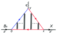
Figure 2: The Feynman diagram for the Coulomb-like interaction.

III Weak decay of $B_{c}$ to P-Wave charmonia

This section is devoted to analyzing the semileptonic and nonleptonic decay processes of $B_{c}$ meson by using the vector and axial vector form factors obtained in previous section.

III.1 Semileptonic decay

The semileptonic decay $B_{c}\to Xl\bar{\nu_{l}}$ $(l=e,\mu$ and $\tau)$ can be described by the following effective Hamiltonian,

$$H_{eff}=\frac{G_{F}}{\sqrt{2}}\sum\limits_{l=e,\mu,\tau}{V_{cb}\bar{c}\gamma_{\mu}(1-\gamma_{5})b\bar{\nu}_{l}\gamma_{\mu}(1-\gamma_{5})l}$$ (30)

where $G_{F}=1.16637\times 10^{-5}$ GeV^-2 is the Fermi constant, $V_{cb}$ is CKM matrix element. The transition matrix element can be written as,

$$T =\left\langle X(p^{\prime})l(l)\bar{v}_{l}(v)\right|H_{eff}\left|B_{c}(p)\right\rangle$$ (31)

$$=\frac{G_{F}}{\sqrt{2}}V_{cb}\left\langle X(p^{\prime})\right|\bar{c}\gamma_{\mu}(1-\gamma_{5})b\left|B_{c}(p)\right\rangle$$

$$\times\left\langle l(l)\bar{v}_{l}(v)\right|\bar{\nu}_{l}\gamma_{\mu}(1-\gamma_{5})l\left|0\right\rangle$$

In the above equation, the $B_{c}\to X$ transition matrix element can be represented as the vector and axial vector form factors. The leptonic matrix element can be formulated as the following form by using perturbative field theory approach,

$$\left\langle l(l)\bar{v}_{l}(v)\right|\bar{\nu}_{l}\gamma_{\mu}(1-\gamma_{5})l\left|0\right\rangle={\bar{u}_{v,s}}\gamma_{\mu}(1-\gamma_{5})u_{-l,s^{\prime}}$$ (32)

where $u_{v,s}$ and $u_{-l,s^{\prime}}$ are the spinor wave functions of $\bar{\nu_{l}}$ and $l$, the subscript $v(l)$ and $s(s^{\prime})$ denote the four momentum and spin of corresponding particles.

III.2 Nonleptonic decay

The nonleptonic decays $B_{c}\to XP$ and $B_{c}\to XV$ where $X$ represent the P-wave charmonia $\chi_{cJ}$ $(J=0,1,2)$ and $h_{c}$, $P$ denote the light pseudoscalar meson $\pi$ or $K$ and $V$ denote the light vector meson $\rho$ or $K^{*}$ can be uniformly described by the following effective Hamiltonian,

$$H_{eff}=\frac{G_{F}}{\sqrt{2}}\sum\limits_{q=d,s}{V_{cb}V_{uq}^{*}a_{1}\bar{c}\gamma_{\mu}(1-\gamma_{5})b\bar{u}\gamma_{\mu}(1-\gamma_{5})q}$$ (33)

where $V_{cb}$ and $V_{uq}$ are CKM matrix elements and $a_{1}$ is the Wilson coefficient. The transition matrix for these decay processes can be expressed as the following form by using the naive factorization approach (NFA) Bauer and Stech (1985); Bauer et al. (1987),

$$T =\left\langle X(p^{\prime})P[V](q)\right|H_{eff}\left|B_{c}(p)\right\rangle$$ (34)

$$=\frac{G_{F}}{\sqrt{2}}V_{cb}V_{uq}^{*}a_{1}\left\langle X(p^{\prime})\right|\bar{c}\gamma_{\mu}(1-\gamma_{5})b\left|B_{c}(p)\right\rangle$$

$$\times\left\langle P[V](q)\right|\bar{u}\gamma_{\mu}(1-\gamma_{5})q\left|0\right\rangle$$

The meson vacuum matrix elements can be defined as the following forms,

$$\left\langle P(q)\right|\bar{u}\gamma_{\mu}(1-\gamma_{5})q\left|0\right\rangle =-if_{P}q_{\mu}$$

$$\left\langle V(q)\right|\bar{u}\gamma_{\mu}(1-\gamma_{5})q\left|0\right\rangle =f_{V}m_{V}\epsilon_{\mu}^{*}$$ (35)

where $f_{P}$ and $f_{V}$ are the decay constants of pseudoscalar and vector meson, $\epsilon_{\mu}$ is the polarization vector of vector meson.

IV Numerical results and discussions

IV.1 Numerical results of form factors

As important input parameters, the heavy quark masses are energy scale dependent, which can be expressed as the following renormalization group equation (RGE),

$$m_{Q}(\mu) =m_{Q}(m_{Q})\left[\frac{\alpha_{s}(\mu)}{\alpha_{s}(m_{Q})}\right]^{\frac{12}{33-2N_{f}}}$$

$$\alpha_{s}(\mu) =\frac{1}{b_{0}t}\left[1-\frac{b_{1}}{b_{0}^{2}}\frac{\log t}{t}\right.$$ (36)

$$\left.+\frac{b_{1}^{2}({\log^{2}}t-\log t-1)+b_{0}b_{2}}{b_{0}^{4}t^{2}}\right]$$

where $t=\log(\frac{\mu^{2}}{\Lambda_{QCD}^{2}})$, $b_{0}=\frac{33-2N_{f}}{12\pi}$, $b_{1}=\frac{153-19N_{f}}{24\pi^{2}}$ and $b_{2}=\frac{2857-\frac{5033}{9}N_{f}+\frac{325}{27}N_{f}^{2}}{128\pi^{3}}$. $\Lambda_{QCD}=213$ MeV for the flavors $N_{f}=5$ in this work Navas et al. (2024). The $\mathrm{\overline{MS}}$ masses of $c$ and $b$ quarks are taken from the Particle Date Group (PDG) Navas et al. (2024), where $m_{c}(m_{c})=1.275\pm 0.025$ GeV and $m_{b}(m_{b})=4.18\pm 0.03$ GeV. Based on our previous works Wang (2024), the energy scale $\mu=2$ GeV works well in $B_{c}$ meson system. Thus, this value is still employed in the present work. The other parameters like masses, decay constants of $B_{c}$ meson and P-wave charmonia and the standard value of vacuum condensate parameter are all listed in Table 1.

Table 1: Input parameters (IP) used to calculate the form factors.

IP	Values (GeV)	IP	Values
$m_{B_{c}}$	6.274 Navas et al. (2024)	$f_{\chi_{c0}}$	0.343 GeV Novikov et al. (1978)
$m_{\chi_{c0}}$	3.414 Navas et al. (2024)	$f_{\chi_{c1}}$	0.338 GeV Novikov et al. (1978)
$m_{\chi_{c1}}$	3.511 Navas et al. (2024)	$f_{h_{c}}$	0.235 GeV Bečirević et al. (2014)
$m_{h_{c}}$	3.525 Navas et al. (2024)	$f_{\chi_{c2}}$	$0.0111\pm 0.0062$ GeV Aliev et al. (2010)
$m_{\chi_{c2}}$	3.556 Navas et al. (2024)	$\langle g_{s}^{2}GG\rangle$	$0.88\pm 0.15$ GeV4 Narison (2010, 2012a, 2012b)
$f_{B_{c}}$	$0.371\pm 0.037$ Wang (2024)

We firstly discuss how the numerical results of formfactors are obtained. From the Eq. (II.2), the form factors depend on some input parameters such as the Borel parameter $T^{2}$, the continuum threshold parameters $s_{0}$ and $u_{0}$, and the square momentum $Q^{2}$. To analyze the corresponding decay processes of $B_{c}$ to charmonia, the values of the form factors in time-like regions ($Q^{2}=-q^{2}<0$) need to be obtained. However, the calculations of three-point QCD sum rules are carried out in space-like regions ($Q^{2}>0$) or $Q^{2}=0$, because of the geometric constraints in Delta function integrals. In addition, some form factors like $F_{0}(Q^{2})$ in Eq. (II.2) have singularity in $Q^{2}=0$. Therefore, we get the values of form factors in space-like regions in this work, and extrapolating them into time-like regions.

To obtain reliable sum rule results, two conditions should be satisfied, which are the pole dominance and convergence of OPE. The pole contribution is defined as Shi et al. (2020),

$$\mathrm{Pole}(T^{2})=\frac{\int_{s_{1}}^{s_{0}}ds\int_{u_{1}}^{u_{0}}du\rho^{QCD}(s,u,Q^{2})e^{-\frac{s}{T^{2}}-\frac{u}{kT^{2}}}}{\int_{s_{1}}^{\infty}ds\int_{u_{1}}^{\infty}du\rho^{QCD}(s,u,Q^{2})e^{-\frac{s}{T^{2}}-\frac{u}{kT^{2}}}}$$

The condition of pole dominance require $\mathrm{Pole}>50\%$. An appropriate work region of Borel parameter should be selected to determine the values of form factors, where the final results are less dependent on the Borel parameter and at the same time the condition of pole dominance is also satisfied. This work region is commonly named as ’Borel platform’. Fixed $Q^{2}=1$ GeV², the Borel parameters are determined and Borel platform is chosen after repeated trial and contrast. The Borel platforms for all form factors are shown in Figs. 8 and 9 in Appendix A. From Figs. 8 and 9, we can see that the non-perturative contribution is tiny, the convergence of OPE is also satisfied. The Borel platform, pole contributions in the Borel platform, and the values of form factors in $Q^{2}=1$ GeV² are listed in Table 2.

Table 2: The Borel platform (BP), pole contributions (PC) and the values of form factors (FF) in $Q^{2}=1$ GeV² for different decay modes. The star denote the results with Coulomb-like correction.

Mode	FF	BP (GeV2)	PC(%)	$F$	$F^{*}$
$B_{c}\to\chi_{c0}$	$F_{0}$	$15\sim 17$	$64\sim 58$	$0.30^{+0.02}_{-0.04}$	$0.84^{+0.06}_{-0.08}$
	$F_{1}$	$15\sim 17$	$63\sim 57$	$0.28^{+0.02}_{-0.03}$	$0.78^{+0.06}_{-0.07}$
	$T$	$18\sim 20$	$73\sim 69$	$0.35^{+0.03}_{-0.04}$	$0.99^{+0.07}_{-0.08}$
$B_{c}\to\chi_{c1}$	$A$	$19\sim 21$	$71\sim 67$	$0.19^{+0.02}_{-0.02}$	$0.53^{+0.04}_{-0.04}$
	$V_{0}$	$23\sim 25$	$79\sim 76$	$0.060^{+0.013}_{-0.012}$	$0.15^{+0.03}_{-0.03}$
	$V_{1}$	$18\sim 20$	$64\sim 59$	$0.51^{+0.05}_{-0.06}$	$1.42^{+0.11}_{-0.13}$
	$V_{2}$	$20\sim 22$	$64\sim 59$	$0.088^{+0.005}_{-0.007}$	$0.26^{+0.01}_{-0.02}$
	$T_{0}$	$19\sim 21$	$76\sim 72$	$0.087^{+0.006}_{-0.008}$	$0.25^{+0.02}_{-0.02}$
	$T_{1}$	$17\sim 19$	$54\sim 50$	$-0.44^{+0.05}_{-0.05}$	$-1.23^{+0.11}_{-0.13}$
	$T_{2}$	$15\sim 17$	$55\sim 50$	$1.23^{+0.12}_{-0.15}$	$3.48^{+0.31}_{-0.34}$
$B_{c}\to h_{c}$	$A$	$9\sim 11$	$55\sim 46$	$0.075^{+0.010}_{-0.011}$	$0.19^{+0.03}_{-0.02}$
	$V_{0}$	$13\sim 15$	$67\sim 61$	$0.80^{+0.07}_{-0.07}$	$2.30^{+0.16}_{-0.18}$
	$V_{1}$	$13\sim 15$	$61\sim 56$	$2.46^{+0.23}_{-0.26}$	$7.05^{+0.56}_{0.65}$
	$V_{2}$	$9\sim 11$	$57\sim 50$	$0.16^{+0.02}_{-0.02}$	$0.46^{+0.05}_{-0.06}$
	$T_{0}$	$16\sim 18$	$90\sim 87$	$0.16^{+0.01}_{-0.02}$	$0.45^{+0.03}_{-0.03}$
	$T_{1}$	$13\sim 15$	$77\sim 72$	$-0.039^{+0.001}_{-0.002}$	$-0.13^{+0.01}_{-0.01}$
	$T_{2}$	$13\sim 15$	$84\sim 78$	$0.49^{+0.02}_{-0.02}$	$1.48^{+0.04}_{-0.05}$
$B_{c}\to\chi_{c2}$	$h$	$18\sim 20$	$70\sim 65$	$0.031^{+0.003}_{-0.003}$	$0.089^{+0.005}_{-0.007}$
	$k$	$13\sim 15$	$76\sim 69$	$1.91^{+0.14}_{-0.17}$	$5.40^{+0.34}_{-0.38}$
	$b_{+}$	$11\sim 13$	$57\sim 52$	$-0.0022^{+0.0003}_{-0.0002}$	$-0.0072^{+0.0005}_{-0.0004}$
	$b_{-}$	$13\sim 15$	$75\sim 66$	$0.018^{+0.001}_{-0.001}$	$0.058^{+0.002}_{-0.002}$
	$T_{0}$	$15\sim 17$	$68\sim 61$	$1.28^{+0.10}_{-0.11}$	$3.66^{+0.24}_{-0.26}$
	$T_{1}$	$13\sim 15$	$67\sim 59$	$0.51^{+0.03}_{-0.05}$	$1.45^{+0.10}_{-0.11}$
	$T_{2}$	$17\sim 19$	$81\sim 76$	$2.00^{+0.17}_{-0.18}$	$5.63^{+0.37}_{-0.43}$

Taking different values of $Q^{2}$, the form factors in space-like regions ($Q^{2}>0$) can be obtained, where the range of $Q^{2}$ is taken as $1\sim 5$ GeV², uniformly. The values of form factors in time-like regions are obtained by fitting the results in space-like regions with appropriate functions and by extrapolating these results into the time-like regions. The $z-$ series parameterization approach was proposed in Ref. Boyd et al. (1995), and was widely employed to fit different form factors Leljak et al. (2019); Bourrely et al. (2009); Zhao et al. (2020); Wang and Shen (2015); Cui et al. (2023). With this method, the form factors can be expanded as the following series,

$$F(Q^{2}) =\frac{1}{1+Q^{2}/m_{R}^{2}}$$ (38)

$$\times\sum\limits_{k=0}^{N-1}{b_{k}\left[z(Q^{2},t_{0})^{k}-{(-1)^{k-N}}\frac{k}{N}\right.}\left.z(Q^{2},t_{0})^{N}\right]$$

where $m_{R}$ is the mass of low-lying $B_{c}$ resonance Leljak et al. (2019) which is taken as 6.75 GeV in the present work. $b_{k}$ is the fitting parameter and the function $z(Q^{2},t_{0})$ is taken as the following form,

$$z(Q^{2},t_{0}) =\frac{\sqrt{t_{+}+Q^{2}}-\sqrt{t_{+}-t_{0}}}{\sqrt{t_{+}+Q^{2}}+\sqrt{t_{+}-t_{0}}}$$ (39)

where $t_{\pm}=(m_{Bc}\pm m_{X})^{2}$, and $t_{0}=t_{+}-\sqrt{t_{+}(t_{+}-t_{-})}$ Leljak et al. (2019); Cui et al. (2023). The $z-$ series are truncated at $N=3$ in our calculation, and the values of fitting parameters $b_{k}$ for all form factors are listed in Table 3. The fitting diagrams of these form factors are shown in Figs. 3$\sim$6.

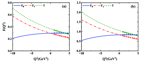
Figure 3: Fitting results of form factors for $B_{c}\to\chi_{c0}$ without cosidering Coulomb-like correction (a) and considering Coulomb-like correction (b).

Table 3: Fitting parameters of different form factors (FF) in $z-$ series expand approach. $b_{k}^{*}$ denote the fitting parameters with Coulomb-like correction.

Mode	FF	$b_{0}$	$b_{1}$	$b_{2}$	$b_{0}^{*}$	$b_{1}^{*}$	$b_{2}^{*}$
$B_{c}\to\chi_{c0}$	$F_{0}$	$0.25$	$4.3$	$-53$	$0.70$	$14$	$-200$
	$F_{1}$	$0.35$	$-5.2$	$34$	$0.99$	$-14$	$75$
	$T$	$0.43$	$-6.2$	$43$	$1.24$	$-17$	$97$
$B_{c}\to\chi_{c1}$	$A$	$0.23$	$-3.3$	$24$	$0.65$	$-8.8$	$48$
	$V_{0}$	$0.073$	$-0.94$	$4.2$	$0.19$	$-2.7$	$14$
	$V_{1}$	$0.42$	$9.0$	$-96$	$1.2$	$26$	$-310$
	$V_{2}$	$0.098$	$-0.71$	$2.9$	$0.29$	$-2.1$	$2.4$
	$T_{0}$	$0.11$	$-2.0$	$17$	$0.32$	$-5.7$	$47$
	$T_{1}$	$-0.55$	$8.9$	$-65$	$-1.6$	$26$	$-190$
	$T_{2}$	$1.5$	$-18$	$101$	$4.2$	$-55$	$320$
$B_{c}\to h_{c}$	$A$	$0.099$	$-1.9$	$14$	$0.26$	$-5.2$	$37$
	$V_{0}$	$1.0$	$-16$	$110$	$2.9$	$-48$	$330$
	$V_{1}$	$2.9$	$-36$	$200$	$8.6$	$-120$	$750$
	$V_{2}$	$0.20$	$-3.5$	$22$	$0.61$	$-13$	$96$
	$T_{0}$	$0.21$	$-4.2$	$38$	$0.60$	$-12$	$110$
	$T_{1}$	$-0.044$	$0.26$	$7.7$	$-0.18$	$3.9$	$-37$
	$T_{2}$	$0.69$	$-16$	$130$	$2.1$	$-51$	$420$
$B_{c}\to\chi_{c2}$	$h$	$0.041$	$-0.80$	$6.6$	$0.12$	$-2.4$	$24$
	$k$	$2.3$	$-30$	$210$	$6.4$	$-79$	$460$
	$b_{+}$	$-0.0019$	$-0.41$	$5.9$	$-0.0046$	$-1.2$	$17$
	$b_{-}$	$0.021$	$-0.16$	$-0.043$	$0.067$	$-0.64$	$1.3$
	$T_{0}$	$2.6$	$-130$	$2100$	$7.5$	$-370$	$6000$
	$T_{1}$	$0.60$	$-6.7$	$19$	$1.7$	$-19$	$54$
	$T_{2}$	$2.6$	$-50$	$460$	$7.2$	$-130$	$1100$

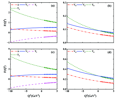
Figure 4: Fitting results of form factors for $B_{c}\to\chi_{c1}$ without considering Coulomb-like correction (a, b) and considering Coulomb-like correction (c, d).

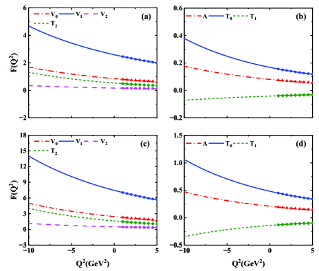
Figure 5: Fitting results of form factors for $B_{c}\to h_{c}$ without considering Coulomb-like correction (a, b) and considering Coulomb-like correction (c, d).

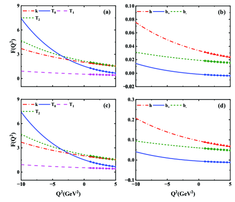
Figure 6: Fitting results of form factors for $B_{c}\to\chi_{c2}$ without cosidering Coulomb-like correction (a, b) and considering Coulomb-like correction (c, d).

The values of form factors at $Q^{2}=0$ are shown in Table 4. As a contrast, the results of other collaborations are also shown in this table. One can find that the form factors with Coulomb-like correction are about three times that of no Coulomb-like correction. For the axial vector form factors $F_{0,1}$ of $B_{c}\to\chi_{c0}$, the axial vector form factor $A$ and vector form factor $V_{2}$ of $B_{c}\to\chi_{c1}$, our results with no Coulomb-like correction are consistent well with those calculated using the Light-front quark model (LFQM) Zhang et al. (2023); Li et al. (2023), but more small for the results given by other LFQM Wang et al. (2009b). After the Coulomb-like correction is considered, our results are larger than their predictions but smaller than the NRQCD predictions Zhu (2018). For the transitions of $B_{c}\to\chi_{c2}$, our predictions of $h$, $b_{+,-}$ without Coumlomb-like correction are compatible with Ref. Wang et al. (2009b), but too larger than Ref. Azizi et al. (2013). For other form factors, various theory predictions are not consistent with each other especially for $B_{c}\to h_{c}$ transitions. In Table 4, we can find that our result for the vector form factor $V_{1}$ of $B_{c}\to h_{c}$ is too larger than other predictions. Moreover, the results for the vector form factor $V_{2}$ are negative in LFQM and NRQCD calculations, but they are positive in QCD sum rules predictions. From Table 4, one can also find that our results are not well compatible with other sum rules predictions. By detailed analysis, we find the main discrepancies originate from different values of the decay constant for hadron, of the energy scale and the type of interpolating currents of $P$-wave charmoina etc. In Ref. Azizi et al. (2009), the vector and axial vector form factors of $B_{c}\to\chi_{c0,1}$ and $h_{c}$ are analyzed with three-point QCD sum rules. In this article, the central values of decay constants for $B_{c}$ and all $P$-wave charmoina are taken as $0.4$ GeV and $0.34$ GeV, the energy scale of heavy quarks is taken as $m_{c}$. In addition, the axial vector current $\bar{c}\gamma_{\mu}\gamma_{5}c$ is selected to interpolate both $\chi_{c1}$ and $h_{c}$. In our present work, the decay constants of $B_{c}$ is taken as $0.371\pm 0.037$ GeV which originates from two-point QCD sum rules calculation considering the next-to-leading contribution of perturbative term Wang (2024), the values of decay constants for $\chi_{c0}$, $\chi_{c1}$ and $h_{c}$ are taken from Refs. Novikov et al. (1978); Bečirević et al. (2014) which are $0.343$, $0.338$ and $0.235$ GeV, the heavy quark energy scale $\mu=2$ GeV is also taken from Ref. Wang (2024). In the present work, we choose the tensor current $\bar{c}\sigma_{\mu\nu}c$ instead of axial vector current to interpolate $h_{c}$ because the quantum number $J^{PC}$ of $h_{c}$ is $1^{+-}$, but the $C$ parity of axial current is $+1$ Wang (2013b). In Ref. Azizi et al. (2013), the vector and axial vector form factors of $B_{c}\to\chi_{c2}$ are analyzed by three-point QCD sum rules, the authors get the QCD spectral density by using Feynman parameterization approach in QCD side. In our analysis, the QCD spectral density is obtained by Cutkoskys’s rules. This is the main reason for the disagreement.

Table 4: The values of the form factors at $Q^{2}=0$. ’This work^∗’ denotes the results with Coulomb-like correction.

Modes	Form factors	This work	This work∗	Azizi et al. (2009, 2013)	Wang et al. (2009b)	Zhang et al. (2023)	Li et al. (2023)	Zhu (2018)
$B_{c}\to\chi_{c0}$	$F_{0}$	$0.29^{+0.03}_{-0.03}$	$0.84^{+0.06}_{-0.08}$	$0.67$	$0.47$	$0.33$	$0.337$	$1.65$
	$F_{1}$	$0.29^{+0.03}_{-0.03}$	$0.83^{+0.07}_{-0.07}$	$0.67$	$0.47$	$0.33$	$0.337$	$1.65$
	$T$	$0.37^{+0.03}_{-0.04}$	$1.05^{+0.07}_{-0.08}$	$-$	$-$	$-$	$-$	$-$
$B_{c}\to\chi_{c1}$	$A$	$0.20^{+0.02}_{-0.02}$	$0.57^{+0.03}_{-0.05}$	$0.13$	$0.36$	$0.24$	$0.215$	$1.24$
	$V_{0}$	$0.064^{+0.013}_{-0.012}$	$0.16^{+0.03}_{-0.03}$	$0.03$	$0.13$	$0.15$	$0.025$	$0.17$
	$V_{1}$	$0.50^{+0.05}_{-0.55}$	$1.40^{+0.12}_{-0.12}$	$0.28$	$0.85$	$0.72$	$0.339$	$2.87$
	$V_{2}$	$0.091^{+0.005}_{-0.006}$	$0.27^{+0.01}_{-0.02}$	$0.059$	$0.15$	$0.10$	$0.078$	$0.57$
	$T_{0}$	$0.093^{+0.006}_{-0.008}$	$0.27^{+0.01}_{-0.02}$	$-$	$-$	$-$	$-$	$-$
	$T_{1}$	$-0.47^{+0.06}_{-0.06}$	$-1.31^{+0.11}_{-0.14}$	$-$	$-$	$-$	$-$	$-$
	$T_{2}$	$1.29^{+0.13}_{-0.14}$	$3.68^{+0.31}_{-0.35}$	$-$	$-$	$-$	$-$	$-$
$B_{c}\to h_{c}$	$A$	$0.081^{+0.010}_{-0.012}$	$0.21^{+0.02}_{-0.02}$	$0.14$	$0.07$	$0.06$	$0.039$	$0.07$
	$V_{0}$	$0.85^{+0.08}_{-0.07}$	$2.46^{+0.16}_{-0.18}$	$0.03$	$0.64$	$0.41$	$0.390$	$2.11$
	$V_{1}$	$2.59^{+0.24}_{-0.26}$	$7.47^{+0.57}_{-0.65}$	$0.29$	$0.50$	$0.42$	$0.298$	$0.54$
	$V_{2}$	$0.17^{+0.02}_{-0.02}$	$0.49^{+0.07}_{-0.05}$	$0.059$	$-0.32$	$-0.18$	$-0.196$	$-0.99$
	$T_{0}$	$0.17^{+0.01}_{-0.02}$	$0.48^{+0.03}_{-0.03}$	$-$	$-$	$-$	$-$	$-$
	$T_{1}$	$-0.041^{+0.002}_{-0.002}$	$-0.14^{+0.00}_{-0.01}$	$-$	$-$	$-$	$-$	$-$
	$T_{2}$	$0.54^{+0.01}_{-0.03}$	$1.62^{+0.04}_{-0.05}$	$-$	$-$	$-$	$-$	$-$
$B_{c}\to\chi_{c2}$	$h$	$0.034^{+0.002}_{-0.003}$	$0.095^{+0.005}_{-0.007}$	$-1.70\times 10^{-4}$	$0.022$	$-$	$-$	$-$
	$k$	$2.01^{+0.15}_{-0.16}$	$5.69^{+0.31}_{-0.38}$	$0.18$	$1.27$	$-$	$-$	$-$
	$b_{+}$	$-0.0016^{+0.0004}_{-0.0001}$	$-0.0057^{+0.0006}_{-0.0002}$	$-0.038$	$-0.011$	$-$	$-$	$-$
	$b_{-}$	$0.019^{+0.001}_{-0.000}$	$0.061^{+0.001}_{-0.002}$	$-0.056$	$0.020$	$-$	$-$	$-$
	$T_{0}$	$1.52^{+0.13}_{-0.10}$	$4.34^{+0.35}_{-0.23}$	$-$	$-$	$-$	$-$	$-$
	$T_{1}$	$0.54^{+0.04}_{-0.05}$	$1.53^{+0.11}_{-0.11}$	$-$	$-$	$-$	$-$	$-$
	$T_{2}$	$2.15^{+0.17}_{-0.19}$	$6.02^{+0.39}_{-0.43}$	$-$	$-$	$-$	$-$	$-$

IV.2 Numerical results of decay widths and branching ratios

With these above form factors, the decay widths and branching ratios of the semileptonic and nonleptonic decays related to $B_{c}$ to $P$-wave charmonia transition are calculated in this section. The relevant input parameters are listed in Table 5.

Table 5: Input parameters (IP) in analysis the decay processes of $B_{c}$ meson.

IP	Values Navas et al. (2024)	IP	Values
$m_{\pi}$	0.140 GeV	$f_{K}$	0.160 GeV Navas et al. (2024)
$m_{K}$	0.494 GeV	$f_{\rho}$	0.216 GeV Navas et al. (2024)
$m_{\rho}$	0.775 GeV	$f_{K^{*}}$	0.217 GeV Navas et al. (2024)
$m_{K^{*}}$	0.892 GeV	$V_{cb}$	0.041 Navas et al. (2024)
$m_{e}$	0.511 MeV	$V_{us}$	0.224 Navas et al. (2024)
$m_{\mu}$	105.7 MeV	$V_{ud}$	0.974 Navas et al. (2024)
$m_{\tau}$	1.78 GeV	$a_{1}$	1.07 Buchalla et al. (1996)
$f_{\pi}$	0.131 GeV

For three-body semileptonic decay $B_{c}\to Xl\bar{\nu}_{l}$ $(l=e,\mu$ and $\tau)$, the differential decay width can be expressed as,

$$d\Gamma(B_{c}\to Xl\bar{\nu}_{l}) =\frac{1}{2J+1}\sum\frac{1}{2m_{B_{c}}}d\Phi(p\to p^{\prime},l,v)|T|^{2}$$

$$d\Phi(p\to p^{\prime},l,v) =(2\pi)^{4}\delta^{4}(p-p^{\prime}-l-v)$$ (40)

$$\times\frac{d^{3}\vec{p}^{\prime}}{(2\pi)^{3}2p^{\prime}_{0}}\frac{d^{3}\vec{l}}{(2\pi)^{3}2l_{0}}\frac{d^{3}\vec{v}}{(2\pi)^{3}2v_{0}}$$

where $J$ is the total angular momentum of $B_{c}$ meson, $\Sigma$ denotes the summation of all the polarization, $d\Phi(p\to p^{\prime},l,v)$ is the three-body phase space, $p$, $p^{\prime}$, $l$ and $v$ are four momentum for $B_{c}$, $X$, $l$ and $\bar{\nu}_{l}$ and $T$ denotes the transition matrix. By inserting intermediate state momentum $q=l+v$, the three-body phase space can be decomposed as product of two-body phase space,

$$d\Phi(p\to p^{\prime},l,v)=\frac{dq^{2}}{2\pi}d\Phi(p\to p^{\prime},q)d\Phi(q\to l,v)$$ (41)

where the two-body space phase $d\Phi(p\to p^{\prime},q)$ can be written as,

$$d\Phi(p\to p^{\prime},q) =(2\pi)^{4}\delta^{4}(p-p^{\prime}-q)\frac{d^{3}\vec{p}^{\prime}}{(2\pi)^{3}2p^{\prime}_{0}}\frac{d^{3}\vec{q}}{(2\pi)^{3}2q_{0}}$$

With the Eqs. (31), (32) and (IV.2) $\sim$ (IV.2), the differential decay widths of $B_{c}\to Xl\bar{\nu}_{l}$ can be obtained. The full expressions are shown in Appendix B. The differential decay widths with variations of $q^{2}$ are shown in Fig. 7. The decay widths and branching ratios for the three-body semileptonic decays can be derived by finishing the integration of $q^{2}$. The numerical results are collected in Table 6. From this table, one can find that $\Gamma(B_{c}\to h_{c}l\bar{\nu}_{l})>\Gamma(B_{c}\to\chi_{c2}l\bar{\nu}_{l})>\Gamma(B_{c}\to\chi_{c0}l\bar{\nu}_{l})>\Gamma(B_{c}\to\chi_{c1}l\bar{\nu}_{l})$ in our prediction, the decay processes of $B_{c}\to h_{c}l\bar{\nu}_{l}$ and $B_{c}\to\chi_{c2}l\bar{\nu}_{l}$ have large branching ratios. Comparing with results in Refs. Azizi et al. (2009, 2013); Ivanov et al. (2006); Hernandez et al. (2006); Wang et al. (2009b); Li et al. (2023); Chang et al. (2002) for the $B_{c}\to\chi_{cJ}l\bar{\nu}_{l}(J=0,1,2)$ and $h_{c}l\bar{\nu}_{l}$ decays which are also collected in Table 6, we can see that most of our results for branching ratios of $B_{c}\to\chi_{c0}l\bar{\nu}_{l}$ and $B_{c}\to\chi_{c1}l\bar{\nu}_{l}$ without Coulomb-like correction are comparable with their predictions. For the branching ratios of $B_{c}\to h_{c}l\bar{\nu}_{l}$ and $B_{c}\to\chi_{c2}l\bar{\nu}_{l}$, our predictions are larger than other collaborations. When we consider the Coulomb-like correction, these results are much larger than other predictions. This is due to the fact that the form factors will be about three times larger after considering the Coulomb-like correction, which will result in about nine times the decay widths and branching ratios. As the next leading order contribution, the Coulomb-like correction is too large. Thus, the results without Coulomb-like correction seem more reasonable. In conclusion, the rigorous calculation of next-to-leading order correction for perturbative contribution of form factors eagerly need to be carried out, and the discrepancies of different theoretical results will be tested by more experiments in the future.

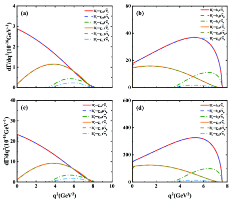
Figure 7: The differential decay width $d\Gamma/dq^{2}$ with variations of $q^{2}$ for semileptonic decay processes $B_{c}\to\chi_{c0}l\nu_{l}$, $\chi_{c1}l\nu_{l}$ and $B_{c}\to h_{c}l\nu_{l}$, $\chi_{c2}l\nu_{l}$ without considering the Coulomb-like correction ((a) and (b)) and considering the Coulomb-like correction ((c) and (d)).

Table 6: Decay widths (in $10^{-6}$eV) and branching ratios ($\%$) of $B_{c}$ semileptonic decays. Branching ratios are calculated at $\tau_{B_{c}}$ = 0.51 ps Navas et al. (2024). The superscript star denotes the results obtained by considering Coulomb-like correction.

Decay channels	Decay widths		Branching ratios
	This work	This work∗	This work	This work∗	Wang et al. (2009b)	Chang et al. (2002)	Ivanov et al. (2006)	Hernandez et al. (2006)	Azizi et al. (2009, 2013)	Li et al. (2023)
$B_{c}^{-}\to\chi_{c0}e\bar{\nu}_{e}$	$1.25^{+0.20}_{-0.24}$	$9.99^{+1.29}_{-1.44}$	$0.097^{+0.016}_{-0.019}$	$0.78^{+0.09}_{-0.12}$	$0.21$	$0.12$	$0.17$	$0.11$	$0.182$	$0.11$
$B_{c}^{-}\to\chi_{c0}\mu\bar{\nu}_{\mu}$	$1.24^{+0.20}_{-0.24}$	$9.93^{+1.26}_{-1.45}$	$0.096^{+0.016}_{-0.018}$	$0.77^{+0.10}_{-0.11}$	$0.21$	$0.12$	$0.17$	$0.11$	$0.182$	$0.11$
$B_{c}^{-}\to\chi_{c0}\tau\bar{\nu}_{\tau}$	$0.14^{+0.02}_{-0.02}$	$1.05^{+0.20}_{-0.08}$	$0.011^{+0.002}_{-0.002}$	$0.082^{+0.015}_{-0.007}$	$0.024$	$0.017$	$0.013$	$0.013$	$0.049$	$0.0094$
$B_{c}^{-}\to\chi_{c1}e\bar{\nu}_{e}$	$0.61^{+0.15}_{-0.10}$	$4.85^{+0.71}_{-0.83}$	$0.047^{+0.012}_{-0.007}$	$0.38^{+0.05}_{-0.07}$	$0.14$	$0.15$	$0.092$	$0.066$	$0.146$	$0.030$
$B_{c}^{-}\to\chi_{c1}\mu\bar{\nu}_{\mu}$	$0.60^{+0.15}_{-0.09}$	$4.82^{+0.70}_{-0.82}$	$0.047^{+0.011}_{-0.007}$	$0.37^{+0.06}_{-0.06}$	$0.14$	$0.15$	$0.092$	$0.066$	$0.146$	$0.029$
$B_{c}^{-}\to\chi_{c1}\tau\bar{\nu}_{\tau}$	$0.064^{+0.018}_{-0.007}$	$0.51^{+0.08}_{-0.08}$	$0.0049^{+0.0014}_{-0.0005}$	$0.039^{+0.007}_{-0.005}$	$0.015$	$0.024$	$0.0089$	$0.0072$	$0.0147$	$0.0026$
$B_{c}^{-}\to h_{c}e\bar{\nu}_{e}$	$22.15^{+3.18}_{-3.43}$	$194.23^{+23.08}_{-24.12}$	$1.72^{+0.24}_{-0.27}$	$15.06^{+1.79}_{-1.87}$	$0.31$	$0.18$	$0.27$	$0.17$	$0.142$	$0.11$
$B_{c}^{-}\to h_{c}\mu\bar{\nu}_{\mu}$	$22.05^{+3.16}_{-3.41}$	$193.31^{+22.98}_{-23.96}$	$1.71^{+0.24}_{-0.27}$	$14.98^{+1.79}_{-1.85}$	$0.31$	$0.18$	$0.27$	$0.17$	$0.142$	$0.11$
$B_{c}^{-}\to h_{c}\tau\bar{\nu}_{\tau}$	$3.03^{+0.36}_{-0.46}$	$26.92^{+3.08}_{-2.66}$	$0.24^{+0.02}_{-0.04}$	$2.09^{+0.24}_{-0.21}$	$0.022$	$0.025$	$0.017$	$0.015$	$0.0137$	$0.0051$
$B_{c}^{-}\to\chi_{c2}e\bar{\nu}_{e}$	$7.93^{+1.14}_{-0.51}$	$61.95^{+8.97}_{-5.69}$	$0.62^{+0.08}_{-0.05}$	$4.80^{+0.70}_{-0.44}$	$0.17$	$0.19$	$0.17$	$0.13$	$0.130$	$-$
$B_{c}^{-}\to\chi_{c2}\mu\bar{\nu}_{\mu}$	$7.85^{+1.13}_{-0.50}$	$61.35^{+8.85}_{-5.65}$	$0.61^{+0.09}_{-0.04}$	$4.76^{+0.68}_{-0.44}$	$0.17$	$0.19$	$0.17$	$0.13$	$0.130$	$-$
$B_{c}^{-}\to\chi_{c2}\tau\bar{\nu}_{\tau}$	$0.43^{+0.03}_{-0.01}$	$3.33^{+0.30}_{-0.38}$	$0.033^{+0.003}_{-0.000}$	$0.26^{+0.02}_{-0.03}$	$0.0092$	$0.029$	$0.0082$	$0.0093$	$0.020$	$-$

For two-body nonleptonic decay $B_{c}\to XP[V]$, the decay width can be expressed by the following standard two-body decay formula,

$$\Gamma =\frac{1}{2J+1}\sum\int\frac{1}{2m_{B_{c}}}d\Phi(p\to p^{\prime},q)|T|^{2}$$ (43)

With the Eqs. (34), (III.2) and (43), the decay widths of $B_{c}\to XP[V]$ can be obtained. The full expressions of decay widths are shown in Appendix C. The numerical results of these two-body decay widths and branching ratios and those of other collaboration’s are explicitly shown in Table 7. It can be seen from Table 7 that the theoretical results of different collaborations are not consistent well with each other. The experimental data for the weak decay of $B_{c}$ to P-wave charmonia are scarce. Only the branching ratios of decay channel $B_{c}\to\chi_{c0}\pi$ is given as $\frac{\sigma(B_{c}^{+})}{\sigma(B^{+})}\times Br(B_{c}^{+}\to\chi_{c0}\pi^{+})=(9.8^{+3.4}_{-3.0}$$($stat$)\pm$0.8$($syst$))\times 10^{-6}$ by the LHCb collaboration Aaij et al. (2015). With our results $Br(B_{c}\to\chi_{c0}\pi)=0.24^{+0.05}_{-0.04}\times 10^{-3}$ without Coulomb-like correction and $1.96^{+0.21}_{-0.30}\times 10^{-3}$ with Coulomb-like correction, the cross section ration $\frac{\sigma(B_{c}^{+})}{\sigma(B^{+})}$ can be extracted to be about $(2\sim 7)\times 10^{-2}$ and $(3\sim 8)\times 10^{-3}$, respectively, which is useful to study the total cross section of $B_{c}$ meson. Overall, further experimental measurements are eagerly awaited to testify the discrepancies of different theoretical predictions.

It is noted that the NFA is adopted to analyze the two-body nonleptonic decays in our present work. However, as the simplest model to study the two-body weak decays of the heavy flavor hadron, NFA does not take into account the hard gloun exchange between the energetic meson emitted from the weak vertex and the $B_{c}$ transition form factors. Thus, the two-body decay width formulas in the framework of NFA are not renormalization invariant, this will lead to systematic uncertainties which are difficult to quantify. Some new factorization techniques such as the QCD factorization (QCDF) Beneke et al. (1999); Beneke and Neubert (2003) and the perturbative QCD factorization (pQCD) Li and Yu (1996); Cheng et al. (1999) methods etc are employed to solve this problem. In the future works, we can try to use these new techniques to improve the accuracy of analysis for $B_{c}$ two-body weak decays.

Table 7: Decay widths (in $10^{-7}$eV) and Branching ratios ($10^{-3}$) of $B_{c}$ nonleptonic decays. The superscript star denotes the results obtained by considering Coulomb-like correction.

Decay channels	Decay widths		Branching ratios
	This work	This work∗	This work	This work∗	Ebert et al. (2010)	Hernandez et al. (2006)	Zhang et al. (2023)	Rui (2018)	Zhu (2018)	Zhu (2018)	Kiselev et al. (2002)
$B_{c}^{-}\to\chi_{c0}\pi^{-}$	$3.11^{+0.65}_{-0.58}$	$25.30^{+3.99}_{-4.07}$	$0.24^{+0.05}_{-0.04}$	$1.96^{+0.21}_{-0.30}$	$0.21$	$0.26$	$0.66$	$1.6$	$4.2$	$6.47$	$9.8$
$B_{c}^{-}\to\chi_{c0}K^{-}$	$0.24^{+0.05}_{-0.04}$	$1.96^{+0.31}_{-0.31}$	$0.019^{+0.004}_{-0.004}$	$0.15^{+0.03}_{-0.02}$	$0.016$	$0.02$	$0.052$	$0.12$	$0.32$	$0.49$	$-$
$B_{c}^{-}\to\chi_{c0}\rho^{-}$	$8.23^{+1.46}_{-1.67}$	$66.60^{+8.88}_{-11.31}$	$0.64^{+0.11}_{-0.13}$	$5.16^{+0.69}_{-0.87}$	$0.58$	$0.67$	$1.69$	$5.8$	$-$	$-$	$33$
$B_{c}^{-}\to\chi_{c0}K^{*-}$	$0.43^{+0.08}_{-0.09}$	$3.49^{+0.46}_{-0.59}$	$0.033^{+0.006}_{-0.006}$	$0.27^{+0.04}_{-0.04}$	$0.04$	$0.037$	$0.096$	$0.33$	$-$	$-$	$-$
$B_{c}^{-}\to\chi_{c1}\pi^{-}$	$0.14^{+0.06}_{-0.05}$	$0.91^{+0.31}_{-0.34}$	$0.011^{+0.005}_{-0.004}$	$0.070^{+0.025}_{-0.026}$	$0.2$	$0.0014$	$0.13$	$0.51$	$0.05$	$0.0064$	$0.089$
$B_{c}^{-}\to\chi_{c1}K^{-}$	$0.011^{+0.004}_{-0.004}$	$0.070^{+0.024}_{-0.026}$	$0.00082^{+0.00038}_{-0.00028}$	$0.0054^{+0.0019}_{-0.0020}$	$0.015$	$0.00011$	$0.010$	$0.038$	$0.004$	$0.00049$	$-$
$B_{c}^{-}\to\chi_{c1}\rho^{-}$	$0.88^{+0.23}_{-0.23}$	$6.74^{+1.05}_{-1.74}$	$0.068^{+0.018}_{-0.018}$	$0.52^{+0.08}_{-0.13}$	$0.15$	$0.10$	$0.43$	$2.8$	$1.47$	$-$	$4.6$
$B_{c}^{-}\to\chi_{c1}K^{*-}$	$0.050^{+0.017}_{-0.010}$	$0.41^{+0.07}_{-0.10}$	$0.0041^{+0.0011}_{-0.0010}$	$0.032^{+0.005}_{-0.008}$	$0.01$	$0.0073$	$0.027$	$0.18$	$0.0707$	$-$	$-$
$B_{c}^{-}\to h_{c}\pi^{-}$	$24.07^{+4.74}_{-3.74}$	$199.98^{+28.92}_{-25.76}$	$1.87^{+0.36}_{-0.29}$	$15.50^{+2.24}_{-1.99}$	$0.46$	$0.53$	$0.96$	$0.54$	$6.2$	$9.73$	$16$
$B_{c}^{-}\to h_{c}K^{-}$	$1.86^{+0.37}_{-0.29}$	$15.48^{+2.20}_{-1.59}$	$0.14^{+0.03}_{-0.02}$	$1.20^{+0.17}_{-0.15}$	$0.035$	$0.041$	$0.075$	$0.043$	$0.47$	$0.74$	$-$
$B_{c}^{-}\to h_{c}\rho^{-}$	$61.36^{+12.36}_{-9.43}$	$523.62^{+65.30}_{-78.40}$	$4.76^{+0.95}_{-0.73}$	$40.59^{+5.06}_{-6.08}$	$1.0$	$1.3$	$2.42$	$2.3$	$1.24$	$-$	$53$
$B_{c}^{-}\to h_{c}K^{*-}$	$3.44^{+0.68}_{-0.53}$	$29.20^{+3.64}_{-4.35}$	$0.27^{+0.05}_{-0.04}$	$2.26^{+0.29}_{-0.33}$	$0.07$	$0.071$	$0.13$	$0.13$	$0.0618$	$-$	$-$
$B_{c}^{-}\to\chi_{c2}\pi^{-}$	$21.41^{+5.38}_{-1.52}$	$168.11^{+40.81}_{-6.55}$	$1.66^{+0.42}_{-0.12}$	$13.03^{+3.17}_{-0.51}$	$0.38$	$0.22$	$-$	$4.0$	$-$	$4.37$	$8.3$
$B_{c}^{-}\to\chi_{c2}K^{-}$	$1.61^{+0.39}_{-0.11}$	$12.65^{+2.99}_{-0.51}$	$0.12^{+0.04}_{-0.01}$	$0.98^{+0.23}_{-0.04}$	$0.028$	$0.017$	$-$	$0.31$	$-$	$0.33$	$-$
$B_{c}^{-}\to\chi_{c2}\rho^{-}$	$57.60^{+12.71}_{-4.47}$	$451.76^{+97.46}_{-24.32}$	$4.47^{+0.98}_{-0.35}$	$35.02^{+7.56}_{-1.88}$	$1.10$	$0.65$	$-$	$16$	$-$	$-$	$33$
$B_{c}^{-}\to\chi_{c2}K^{*-}$	$3.05^{+0.64}_{-0.24}$	$23.91^{+4.96}_{-1.40}$	$0.24^{+0.05}_{-0.02}$	$1.85^{+0.39}_{-0.10}$	$0.074$	$0.038$	$-$	$0.96$	$-$	$-$	$-$

V Conclusions

In this work, the vector, axial vector and tensor form factors of $B_{c}$ to $P$-wave charmonia in space-like regions are firstly analyzed in three-point QCD sum rules where the contribution of gluon condensate and Coulomb-like correction are considered. Then, these form factors in zero point and time-like regions are obtained by fitting the results within $z-$ series parameterization approach. With calculated vector and axial vector form factors, we directly analyze the three-body semileptonic decay processes of $B_{c}$ to $P$-wave charmonia. In addition, the two-body nonleptonic decay processes of $B_{c}$ to $P$-wave charmonia and light pseudoscalar or vector mesons are also analyzed by using NFA. We hope these results can help to shed more light on the properties of $B_{c}$ meson and $P$-wave charmonia and provide useful information to research the heavy-flavor physics.

Appendix A The graphics of Borel platforms for all form factors.

See Figs. 8 and 9.

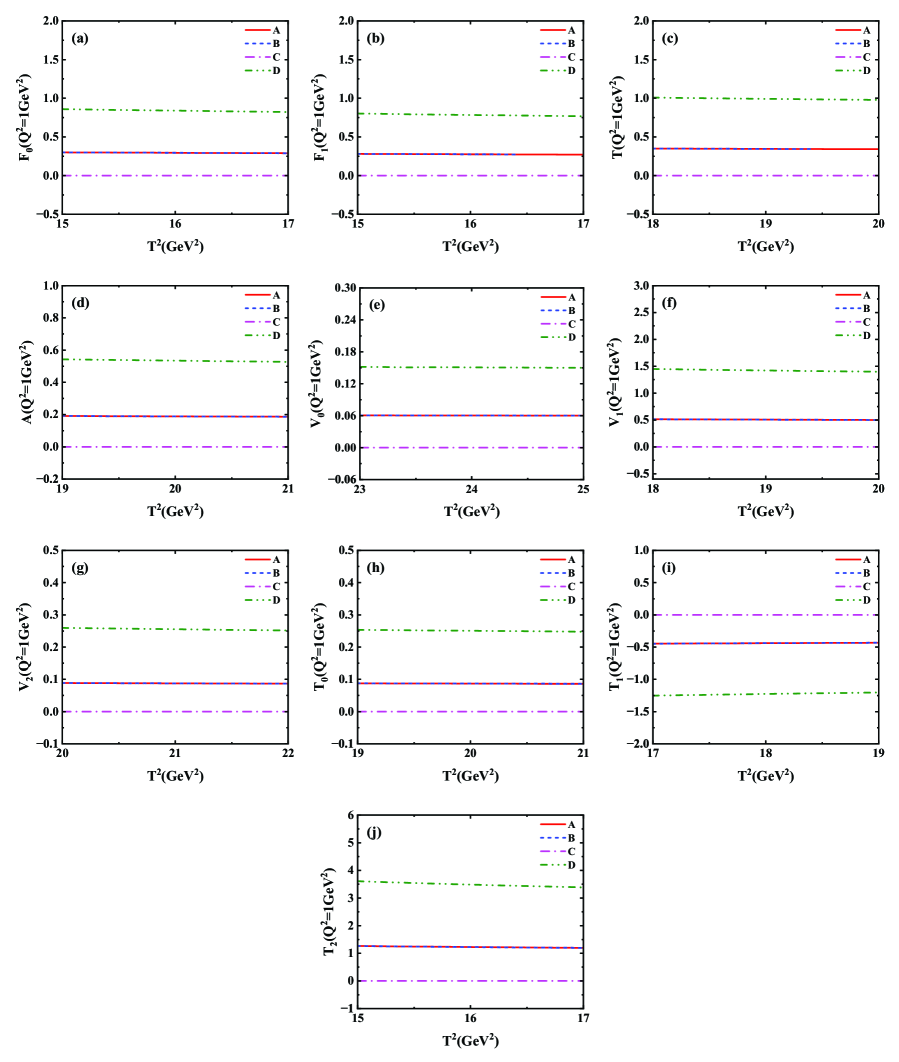
Figure 8: The contributions of perturbative and non-perturbative terms with variation of Borel parameter $T^{2}$. (a-c) are for axial vector and tensor form factors of $B_{c}\to\chi_{c0}$, (d-j) are for axial vector, vector and tensor form factors of $B_{c}\to\chi_{c1}$. The legends A-C denote the total, perturbative, gluon condensate contributions, and D represent the total contribution by considering the Coulomb-like correction.

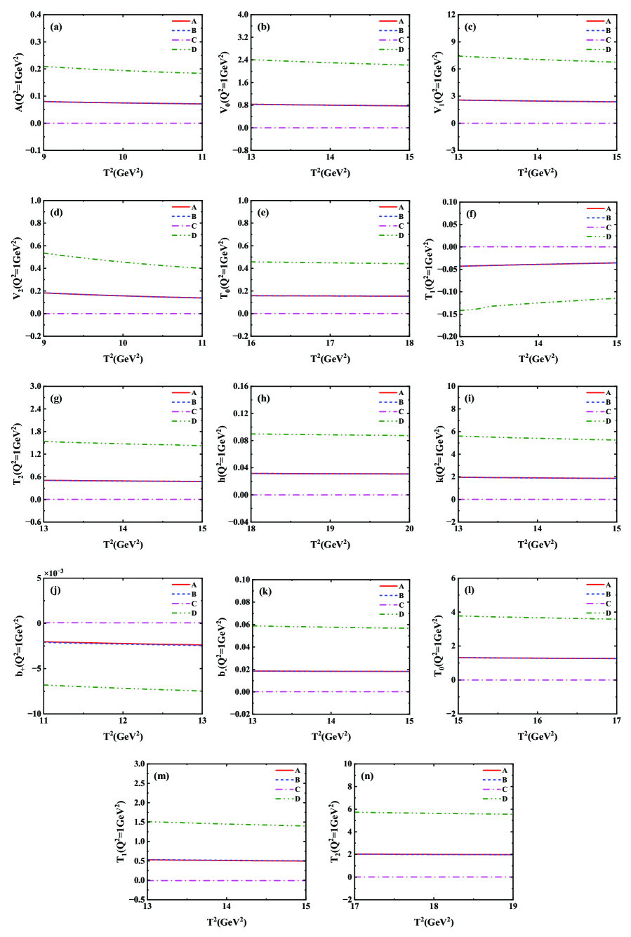
Figure 9: The contributions of perturbative and non-perturbative terms with variation of Borel parameter $T^{2}$. (a-g) are for axial vector, vector and tensor form factors of $B_{c}\to h_{c}$ and (h-n) are for axial vector, vector and tensor form factors of $B_{c}\to\chi_{c2}$. The legends are same as Fig. 8.

Appendix B The full expressions of differential decay widths for $B_{c}$ semileptonic decays.

The differential decay width of $B_{c}\to\chi_{c0}l\bar{\nu}_{l}$ can be expressed as,

$$\frac{d\Gamma(B_{c}\to\chi_{c0}l\bar{\nu}_{l})}{dq^{2}} =\big{(}\frac{q^{2}-m_{l}^{2}}{q^{2}}\big{)}^{2}\frac{G_{F}^{2}V_{cb}^{2}\lambda(m_{B_{c}}^{2},m_{\chi_{c0}}^{2},q^{2})^{1/2}}{384\pi^{3}m_{B_{c}}^{3}q^{2}}\left[(m_{l}^{2}+2q^{2})\lambda(m_{B_{c}}^{2},m_{\chi_{c0}}^{2},q^{2})F_{1}(q^{2})^{2}\right.$$ (44)

$$\left.+3m_{l}^{2}(m_{B_{c}}^{2}-m_{\chi_{c0}}^{2})^{2}F_{0}(q^{2})^{2}\right]$$

where the lambda function can be defined as,

$$\lambda(a,b,c)=a^{2}+b^{2}+c^{2}-2(ab+ac+bc)$$ (45)

The expressions of differential decay width for $B_{c}\to\chi_{c1}[h_{c}]l\bar{\nu}_{l}$ is as follow,

$$\frac{d\Gamma(B_{c}\to\chi_{c1}[h_{c}]l{\bar{\nu}_{l}})}{dq^{2}}=\frac{d\Gamma^{L}(B_{c}\to\chi_{c1}[h_{c}]l\bar{\nu}_{l})}{dq^{2}}+\frac{d\Gamma^{+}(B_{c}\to\chi_{c1}[h_{c}]l\bar{\nu}_{l})}{dq^{2}}+\frac{d\Gamma^{-}(B_{c}\to\chi_{c1}[h_{c}]l\bar{\nu}_{l})}{dq^{2}}$$ (46)

where,

$$\frac{d\Gamma^{L}(B_{c}\to\chi_{c1}[h_{c}]l\bar{\nu}_{l})}{dq^{2}} =\big{(}\frac{q^{2}-m_{l}^{2}}{q^{2}}\big{)}^{2}\frac{G_{F}^{2}V_{cb}^{2}\lambda(m_{B_{c}}^{2},m_{\chi_{c1}[h_{c}]}^{2},q^{2})^{1/2}}{384\pi^{3}m_{B_{c}}^{3}q^{2}}\left\{3m_{l}^{2}\lambda(m_{B_{c}}^{2},m_{\chi_{c1}[h_{c}]}^{2},q^{2})V_{0}(q^{2})^{2}+\frac{m_{l}^{2}+2q^{2}}{4m_{\chi_{c1}[h_{c}]}^{2}}\right.$$

$$\times\left.\left.\left[(m_{B_{c}}^{2}-m_{\chi_{c1}[h_{c}]}^{2}-q^{2})\right.(m_{B_{c}}-m_{\chi_{c1}[h_{c}]})V_{1}(q^{2})-\frac{\lambda(m_{B_{c}}^{2},m_{\chi_{c1}[h_{c}]}^{2},q^{2})}{m_{B_{c}}-m_{\chi_{c1}[h_{c}]}}V_{2}(q^{2})\right]^{2}\right\}$$

$$\frac{d\Gamma^{\pm}(B_{c}\to\chi_{c1}[h_{c}]l\bar{\nu}_{l})}{dq^{2}} =\big{(}\frac{q^{2}-m_{l}^{2}}{q^{2}}\big{)}^{2}\frac{G_{F}^{2}V_{cb}^{2}\lambda(m_{B_{c}}^{2},m_{\chi_{c1}[h_{c}]}^{2},q^{2})^{1/2}}{384\pi^{3}m_{B_{c}}^{3}}\left\{(m_{l}^{2}+2q^{2})\lambda(m_{B_{c}}^{2},m_{\chi_{c1}[h_{c}]}^{2},q^{2})\right.$$ (47)

$$\times\left.\left[\frac{A(q^{2})}{m_{B_{c}}-m_{\chi_{c1}[h_{c}]}}\left.\mp\frac{(m_{B_{c}}-m_{\chi_{c1}}[h_{c}])V_{1}(q^{2})}{\lambda(m_{B_{c}}^{2},m_{\chi_{c1}[h_{c}]}^{2},q^{2})^{1/2}}\right]\right.^{2}\right\}$$

The differential decay width of $B_{c}\to\chi_{c2}l\bar{\nu}_{l}$ can be expressed as,

$$\frac{d\Gamma(B_{c}\to\chi_{c2}l\bar{\nu}_{l})}{dq^{2}}=\frac{d\Gamma^{L}(B_{c}\to\chi_{c2}l\bar{\nu}_{l})}{dq^{2}}+\frac{d\Gamma^{+}(B_{c}\to\chi_{c2}l\bar{\nu}_{l})}{dq^{2}}+\frac{d\Gamma^{-}(B_{c}\to\chi_{c2}l\bar{\nu}_{l})}{dq^{2}}$$ (48)

where,

$$\frac{d\Gamma^{L}(B_{c}\to\chi_{c2}l\bar{\nu}_{l})}{dq^{2}} =\big{(}\frac{q^{2}-m_{l}^{2}}{q^{2}}\big{)}^{2}\frac{G_{F}^{2}V_{cb}^{2}\lambda(m_{B_{c}}^{2},m_{\chi_{c2}}^{2},q^{2})^{3/2}}{3072\pi^{3}m_{B_{c}}^{3}m_{\chi_{c2}}^{2}q^{2}}\left\{3m_{l}^{2}\lambda(m_{B_{c}}^{2},m_{\chi_{c2}}^{2},q^{2})V_{0}(q^{2})^{2}+\frac{m_{l}^{2}+2q^{2}}{4m_{\chi_{c2}}^{2}}\right.$$

$$\times\left.\left[(m_{B_{c}}^{2}-m_{\chi_{c2}}^{2}-q^{2})\right.(m_{B_{c}}-m_{\chi_{c2}})V_{1}(q^{2})\left.\left.-\frac{\lambda(m_{B_{c}}^{2},m_{\chi_{c2}}^{2},q^{2})}{m_{B_{c}}-m_{\chi_{c2}}}V_{2}(q^{2})\right]^{2}\right.\right\}$$

$$\frac{d\Gamma^{\pm}(B_{c}\to\chi_{c2}l\bar{\nu}_{l})}{dq^{2}} =(\frac{q^{2}-m_{l}^{2}}{q^{2}})^{2}\frac{G_{F}^{2}V_{cb}^{2}\lambda(m_{B_{c}}^{2},m_{\chi_{c2}}^{2},q^{2})^{3/2}}{2304\pi^{3}m_{\chi_{c2}}^{2}m_{B_{c}}^{3}}\left\{(m_{l}^{2}+2q^{2})\lambda(m_{B_{c}}^{2},m_{\chi_{c2}}^{2},q^{2})\right.$$ (49)

$$\times\left.\left[\frac{A(q^{2})}{m_{B_{c}}-m_{\chi_{c2}}}\left.\mp\frac{(m_{B_{c}}-m_{\chi_{c2}})V_{1}(q^{2})}{\lambda(m_{B_{c}}^{2},m_{\chi_{c2}}^{2},q^{2})^{1/2}}\right]\right.^{2}\right\}$$

The definitions of form factors $A$, $V_{0}$, $V_{1}$ and $V_{2}$ for $B_{c}\to\chi_{c2}$ are given by Eq. (II.1).

Appendix C The full expressions of decay widths for $B_{c}$ nonleptonic decays.

The full expressions of decay widths for two-body nonleptonic decays $B_{c}\to XP$ and $B_{c}\to XV$ are as follows,

$$\Gamma(B_{c}\to\chi_{c0}P) =\frac{G_{F}^{2}f_{P}^{2}V_{cb}^{2}V_{uq}^{2}\lambda(m_{B_{c}}^{2},m_{\chi_{c0}}^{2},m_{P}^{2})^{1/2}}{32\pi m_{B_{c}}^{3}}a_{1}^{2}F_{0}(m_{P}^{2})^{2}\big{(}m_{B_{c}}^{2}-m_{\chi_{c0}}^{2}\big{)}^{2}$$

$$\Gamma(B_{c}\to\chi_{c0}V) =\frac{G_{F}^{2}f_{V}^{2}V_{cb}^{2}V_{uq}^{2}\lambda(m_{B_{c}}^{2},m_{\chi_{c0}}^{2},m_{V}^{2})^{3/2}}{32\pi m_{B_{c}}^{3}}a_{1}^{2}F_{1}(m_{V}^{2})^{2}$$ (50)

$$\Gamma(B_{c}\to\chi_{c1}[h_{c}]P) =\frac{G_{F}^{2}f_{P}^{2}V_{cb}^{2}V_{uq}^{2}\lambda(m_{B_{c}}^{2},m_{\chi_{c1}[h_{c}]}^{2},m_{P}^{2})^{3/2}}{32\pi m_{B_{c}}^{3}}a_{1}^{2}V_{0}(m_{P}^{2})^{2}$$

$$\Gamma(B_{c}\to\chi_{c1}[h_{c}]V) =\Gamma^{L}(B_{c}\to\chi_{c1}[h_{c}]V)+\Gamma^{+}(B_{c}\to\chi_{c1}[h_{c}]V)+\Gamma^{-}(B_{c}\to\chi_{c1}[h_{c}]V)$$ (51)

where,

$$\Gamma^{L}(B_{c}\to\chi_{c1}[h_{c}]V) =\frac{\lambda(m_{B_{c}}^{2},m_{\chi_{c1}[h_{c}]}^{2},m_{V}^{2})^{1/2}}{32\pi m_{B_{c}}^{3}}G_{F}^{2}V_{cb}^{2}V_{uq}^{2}f_{V}^{2}m_{V}^{2}a_{1}^{2}\left[(m_{B_{c}}-m_{\chi_{c1}[h_{c}]})\frac{m_{B_{c}}^{2}-m_{\chi_{c1}[h_{c}]}^{2}-m_{V}^{2}}{2m_{\chi_{c1}[h_{c}]}m_{V}}V_{1}(m_{V}^{2})\right.$$

$$\left.-\frac{\lambda(m_{B_{c}}^{2},m_{\chi_{c1}[h_{c}]}^{2},m_{V}^{2})}{2m_{\chi_{c1}[h_{c}]}m_{V}(m_{B_{c}}-m_{\chi_{c1}}[h_{c}])}V_{2}(m_{V}^{2})\right]^{2}$$

$$\Gamma^{\pm}(B_{c}\to\chi_{c1}[h_{c}]V) =\frac{\lambda(m_{B_{c}}^{2},m_{\chi_{c1}[h_{c}]}^{2},m_{V}^{2})^{1/2}}{32\pi m_{B_{c}}^{3}}G_{F}^{2}V_{cb}^{2}V_{uq}^{2}f_{V}^{2}m_{V}^{2}a_{1}^{2}\left[(m_{B_{c}}-m_{\chi_{c1}})V_{1}(m_{V}^{2})\right.$$ (52)

$$\mp\left.\frac{\lambda(m_{B_{c}}^{2},m_{\chi_{c1}[h_{c}]}^{2},m_{V}^{2})^{1/2}}{2(m_{B_{c}}-m_{\chi_{c1}})}A(m_{V}^{2})\right]^{2}$$

$$\Gamma(B_{c}\to\chi_{c2}P) =\frac{G_{F}^{2}f_{P}^{2}V_{cb}^{2}V_{uq}^{2}\lambda(m_{B_{c}}^{2},m_{\chi_{c2}}^{2},m_{P}^{2})^{5/2}}{192\pi m_{B_{c}}^{3}m_{\chi_{c2}}^{2}}a_{1}^{2}V_{0}(m_{P}^{2})^{2}$$

$$\Gamma(B_{c}\to\chi_{c2}V) =\Gamma^{L}(B_{c}\to\chi_{c2}V)+\Gamma^{+}(B_{c}\to\chi_{c2}V)+\Gamma^{-}(B_{c}\to\chi_{c2}V)$$ (53)

where,

$$\Gamma^{L}(B_{c}\to\chi_{c2}V) =\frac{\lambda(m_{B_{c}}^{2},m_{\chi_{c2}}^{2},m_{V}^{2})^{3/2}}{192\pi m_{B_{c}}^{3}m_{\chi_{c2}}^{2}}G_{F}^{2}V_{cb}^{2}V_{uq}^{2}f_{V}^{2}m_{V}^{2}a_{1}^{2}\left[(m_{B_{c}}-m_{\chi_{c2}})\frac{m_{B_{c}}^{2}-m_{\chi_{c2}}^{2}-m_{V}^{2}}{2m_{\chi_{c2}}m_{V}}V_{1}(m_{V}^{2})\right.$$

$$\left.-\frac{\lambda(m_{B_{c}}^{2},m_{\chi_{c2}}^{2},m_{V}^{2})}{2m_{\chi_{c2}}m_{V}(m_{B_{c}}-m_{\chi_{c2}})}V_{2}(m_{V}^{2})\right]^{2}$$

$$\Gamma^{\pm}(B_{c}\to\chi_{c2}V) =\frac{\lambda(m_{B_{c}}^{2},m_{\chi_{c2}}^{2},m_{P}^{2})^{3/2}}{256\pi m_{B_{c}}^{3}m_{\chi_{c2}}^{2}}G_{F}^{2}V_{cb}^{2}V_{uq}^{2}f_{V}^{2}m_{V}^{2}a_{1}^{2}\left[(m_{B_{c}}-m_{\chi_{c2}})V_{1}(m_{V}^{2})\right.$$ (54)

$$\mp\left.\frac{\lambda(m_{B_{c}}^{2},m_{\chi_{c2}}^{2},m_{V}^{2})^{1/2}}{2(m_{B_{c}}-m_{\chi_{c2}})}A(m_{V}^{2})\right]^{2}$$

References

- Abe et al. (1998) F. Abe et al. (CDF), Phys. Rev. D 58, 112004 (1998), eprint hep-ex/9804014.
- Chang and Chen (1994) C.-H. Chang and Y.-Q. Chen, Phys. Rev. D 49, 3399 (1994).
- Chang et al. (1998) C.-H. Chang, J.-P. Cheng, and C.-D. Lu, Phys. Lett. B 425, 166 (1998), eprint hep-ph/9712325.
- Gao et al. (2010) Y.-N. Gao, J. He, P. Robbe, M.-H. Schune, and Z.-W. Yang, Chin. Phys. Lett. 27, 061302 (2010).
- Colquhoun et al. (2016) B. Colquhoun, C. Davies, J. Koponen, A. Lytle, and C. McNeile (HPQCD), PoS LATTICE2016, 281 (2016), eprint 1611.01987.
- Harrison et al. (2020) J. Harrison, C. T. H. Davies, and A. Lytle (HPQCD), Phys. Rev. D 102, 094518 (2020), eprint 2007.06957.
- Colangelo et al. (1993) P. Colangelo, G. Nardulli, and N. Paver, Z. Phys. C 57, 43 (1993).
- Kiselev et al. (2000) V. V. Kiselev, A. E. Kovalsky, and A. K. Likhoded, Nucl. Phys. B 585, 353 (2000), eprint hep-ph/0002127.
- Azizi et al. (2009) K. Azizi, H. Sundu, and M. Bayar, Phys. Rev. D 79, 116001 (2009), eprint 0902.1467.
- Azizi et al. (2013) K. Azizi, Y. Sarac, and H. Sundu, Eur. Phys. J. C 73, 2638 (2013), eprint 1306.4095.
- Wu et al. (2024) B. Wu, G.-L. Yu, J. Lu, and Z.-G. Wang, Phys. Lett. B 859, 139118 (2024), eprint 2406.08181.
- Huang and Zuo (2007) T. Huang and F. Zuo, Eur. Phys. J. C 51, 833 (2007), eprint hep-ph/0702147.
- Wang and Lu (2008) Y.-M. Wang and C.-D. Lu, Phys. Rev. D 77, 054003 (2008), eprint 0707.4439.
- Leljak et al. (2019) D. Leljak, B. Melic, and M. Patra, JHEP 05, 094 (2019), eprint 1901.08368.
- Bordone et al. (2023) M. Bordone, A. Khodjamirian, and T. Mannel, JHEP 01, 032 (2023), eprint 2209.08851.
- Kiselev et al. (2002) V. V. Kiselev, O. N. Pakhomova, and V. A. Saleev, J. Phys. G 28, 595 (2002), eprint hep-ph/0110180.
- Rui (2018) Z. Rui, Phys. Rev. D 97, 033001 (2018), eprint 1712.08928.
- Liu et al. (2018) X. Liu, H.-n. Li, and Z.-J. Xiao, Phys. Rev. D 97, 113001 (2018), eprint 1801.06145.
- Liu et al. (2020) X. Liu, H.-n. Li, and Z.-J. Xiao, Phys. Lett. B 811, 135892 (2020), eprint 2006.12786.
- Nobes and Woloshyn (2000) M. A. Nobes and R. M. Woloshyn, J. Phys. G 26, 1079 (2000), eprint hep-ph/0005056.
- Ivanov et al. (2006) M. A. Ivanov, J. G. Korner, and P. Santorelli, Phys. Rev. D 73, 054024 (2006), eprint hep-ph/0602050.
- Ebert et al. (2010) D. Ebert, R. N. Faustov, and V. O. Galkin, Phys. Rev. D 82, 034019 (2010), eprint 1007.1369.
- Hernandez et al. (2006) E. Hernandez, J. Nieves, and J. M. Verde-Velasco, Phys. Rev. D 74, 074008 (2006), eprint hep-ph/0607150.
- Wang et al. (2009a) W. Wang, Y.-L. Shen, and C.-D. Lu, Phys. Rev. D 79, 054012 (2009a), eprint 0811.3748.
- Wang et al. (2009b) X.-X. Wang, W. Wang, and C.-D. Lu, Phys. Rev. D 79, 114018 (2009b), eprint 0901.1934.
- Zhang et al. (2023) Z.-Q. Zhang, Z.-J. Sun, Y.-C. Zhao, Y.-Y. Yang, and Z.-Y. Zhang, Eur. Phys. J. C 83, 477 (2023), eprint 2301.11107.
- Li et al. (2023) X.-J. Li, Y.-S. Li, F.-L. Wang, and X. Liu, Eur. Phys. J. C 83, 1080 (2023), eprint 2308.07206.
- Qiao et al. (2014) C.-F. Qiao, P. Sun, D. Yang, and R.-L. Zhu, Phys. Rev. D 89, 034008 (2014), eprint 1209.5859.
- Zhu (2018) R. Zhu, Nucl. Phys. B 931, 359 (2018), eprint 1710.07011.
- Tang et al. (2022) R.-Y. Tang, Z.-R. Huang, C.-D. Lü, and R. Zhu, J. Phys. G 49, 115003 (2022), eprint 2204.04357.
- Chang et al. (2002) C.-H. Chang, Y.-Q. Chen, G.-L. Wang, and H.-S. Zong, Phys. Rev. D 65, 014017 (2002), eprint hep-ph/0103036.
- Tran et al. (2018) C.-T. Tran, M. A. Ivanov, J. G. Körner, and P. Santorelli, Phys. Rev. D 97, 054014 (2018), eprint 1801.06927.
- Wei et al. (2007) W. Wei, X. Liu, and S.-L. Zhu, Phys. Rev. D 75, 014013 (2007), eprint hep-ph/0612066.
- Wang (2013a) Z.-G. Wang, JHEP 10, 208 (2013a), eprint 1301.1399.
- Chen et al. (2015) H.-X. Chen, W. Chen, Q. Mao, A. Hosaka, X. Liu, and S.-L. Zhu, Phys. Rev. D 91, 054034 (2015), eprint 1502.01103.
- Wang (2015) Z.-G. Wang, Eur. Phys. J. C 75, 427 (2015), eprint 1506.01993.
- Chen et al. (2016) H.-X. Chen, Q. Mao, A. Hosaka, X. Liu, and S.-L. Zhu, Phys. Rev. D 94, 114016 (2016), eprint 1611.02677.
- Zhang et al. (2021) Y. Zhang, T. Zhong, H.-B. Fu, W. Cheng, and X.-G. Wu, Phys. Rev. D 103, 114024 (2021), eprint 2104.00180.
- Wang (2022) Z.-G. Wang, Nucl. Phys. B 985, 115983 (2022), eprint 2207.08059.
- Huang et al. (2023) D. Huang, T. Zhong, H.-B. Fu, Z.-H. Wu, X.-G. Wu, and H. Tong, Eur. Phys. J. C 83, 680 (2023), eprint 2211.06211.
- Su et al. (2024) N. Su, H.-X. Chen, P. Gubler, and A. Hosaka, Phys. Rev. D 110, 034007 (2024), eprint 2405.06958.
- Wang (2024) Z.-G. Wang, Chin. Phys. C 48, 103104 (2024), eprint 2401.12571.
- Wang et al. (2008) Y.-M. Wang, H. Zou, Z.-T. Wei, X.-Q. Li, and C.-D. Lu, Eur. Phys. J. C 54, 107 (2008), eprint 0707.1138.
- Wang et al. (2009c) Y.-M. Wang, H. Zou, Z.-T. Wei, X.-Q. Li, and C.-D. Lu, J. Phys. G 36, 105002 (2009c), eprint 0810.3586.
- Shi et al. (2020) Y.-J. Shi, W. Wang, and Z.-X. Zhao, Eur. Phys. J. C 80, 568 (2020), eprint 1902.01092.
- Peng and Yang (2020) Y.-Q. Peng and M.-Z. Yang, Commun. Theor. Phys. 72, 095201 (2020), eprint 2001.08459.
- Zhao et al. (2020) Z.-X. Zhao, R.-H. Li, Y.-L. Shen, Y.-J. Shi, and Y.-S. Yang, Eur. Phys. J. C 80, 1181 (2020), eprint 2010.07150.
- Neishabouri et al. (2024) Z. Neishabouri, K. Azizi, and H. R. Moshfegh, Phys. Rev. D 110, 014010 (2024), eprint 2404.12654.
- Tousi et al. (2024) M. S. Tousi, K. Azizi, and H. R. Moshfegh, Phys. Rev. D 110, 114001 (2024), eprint 2409.00241.
- Lu et al. (2024) J. Lu, G.-L. Yu, Z.-G. Wang, and B. Wu, Phys. Lett. B 852, 138624 (2024), eprint 2401.00669.
- Bracco et al. (2012) M. E. Bracco, M. Chiapparini, F. S. Navarra, and M. Nielsen, Prog. Part. Nucl. Phys. 67, 1019 (2012), eprint 1104.2864.
- Wang (2014) Z.-G. Wang, Phys. Rev. D 89, 034017 (2014), eprint 1307.2422.
- Azizi et al. (2014) K. Azizi, Y. Sarac, and H. Sundu, Phys. Rev. D 90, 114011 (2014), eprint 1410.7548.
- Azizi et al. (2015) K. Azizi, Y. Sarac, and H. Sundu, Nucl. Phys. A 943, 159 (2015), eprint 1501.05084.
- Yu et al. (2015) G.-L. Yu, Z.-Y. Li, and Z.-G. Wang, Eur. Phys. J. C 75, 243 (2015), eprint 1502.01698.
- Rodrigues et al. (2017) B. O. Rodrigues, M. E. Bracco, and C. M. Zanetti, Nucl. Phys. A 966, 208 (2017), eprint 1707.02330.
- Yu et al. (2019) G.-L. Yu, Z.-G. Wang, and Z.-Y. Li, Eur. Phys. J. C 79, 798 (2019), eprint 1905.11236.
- Lu et al. (2023a) J. Lu, G.-L. Yu, and Z.-G. Wang, Eur. Phys. J. A 59, 195 (2023a), eprint 2304.13969.
- Lu et al. (2023b) J. Lu, G.-L. Yu, Z.-G. Wang, and B. Wu, Eur. Phys. J. C 83, 907 (2023b), eprint 2308.06705.
- Wang (2018) Z.-G. Wang, Eur. Phys. J. C 78, 297 (2018), eprint 1712.05664.
- Dehghan et al. (2023) Z. Dehghan, K. Azizi, and U. Özdem, Phys. Rev. D 108, 094037 (2023), eprint 2307.14880.
- Özdem and Azizi (2024) U. Özdem and K. Azizi, Phys. Rev. D 109, 114019 (2024), eprint 2401.04798.
- Colangelo and Khodjamirian (2000) P. Colangelo and A. Khodjamirian, pp. 1495–1576 (2000), eprint hep-ph/0010175.
- Wirbel et al. (1985) M. Wirbel, B. Stech, and M. Bauer, Z. Phys. C 29, 637 (1985).
- Colangelo et al. (2022) P. Colangelo, F. De Fazio, N. Losacco, F. Loparco, and M. Novoa-Brunet, Phys. Rev. D 106, 094005 (2022), eprint 2208.13398.
- Bracco et al. (1999) M. E. Bracco, F. S. Navarra, and M. Nielsen, Phys. Lett. B 454, 346 (1999), eprint nucl-th/9902007.
- Wang and Di (2014) Z.-G. Wang and Z.-Y. Di, Eur. Phys. J. A 50, 143 (2014), eprint 1405.5092.
- Ioffe and Smilga (1983) B. L. Ioffe and A. V. Smilga, Nucl. Phys. B 216, 373 (1983).
- Bauer and Stech (1985) M. Bauer and B. Stech, Phys. Lett. B 152, 380 (1985).
- Bauer et al. (1987) M. Bauer, B. Stech, and M. Wirbel, Z. Phys. C 34, 103 (1987).
- Navas et al. (2024) S. Navas et al. (Particle Data Group), Phys. Rev. D 110, 030001 (2024).
- Novikov et al. (1978) V. A. Novikov, L. B. Okun, M. A. Shifman, A. I. Vainshtein, M. B. Voloshin, and V. I. Zakharov, Phys. Rept. 41, 1 (1978).
- Bečirević et al. (2014) D. Bečirević, G. Duplančić, B. Klajn, B. Melić, and F. Sanfilippo, Nucl. Phys. B 883, 306 (2014), eprint 1312.2858.
- Aliev et al. (2010) T. M. Aliev, K. Azizi, and M. Savci, Phys. Lett. B 690, 164 (2010), eprint 1002.2767.
- Narison (2010) S. Narison, Phys. Lett. B 693, 559 (2010), [Erratum: Phys.Lett.B 705, 544–544 (2011)], eprint 1004.5333.
- Narison (2012a) S. Narison, Phys. Lett. B 706, 412 (2012a), eprint 1105.2922.
- Narison (2012b) S. Narison, Phys. Lett. B 707, 259 (2012b), eprint 1105.5070.
- Boyd et al. (1995) C. G. Boyd, B. Grinstein, and R. F. Lebed, Phys. Rev. Lett. 74, 4603 (1995), eprint hep-ph/9412324.
- Bourrely et al. (2009) C. Bourrely, I. Caprini, and L. Lellouch, Phys. Rev. D 79, 013008 (2009), [Erratum: Phys.Rev.D 82, 099902 (2010)], eprint 0807.2722.
- Wang and Shen (2015) Y.-M. Wang and Y.-L. Shen, Nucl. Phys. B 898, 563 (2015), eprint 1506.00667.
- Cui et al. (2023) B.-Y. Cui, Y.-K. Huang, Y.-L. Shen, C. Wang, and Y.-M. Wang, JHEP 03, 140 (2023), eprint 2212.11624.
- Wang (2013b) Z.-G. Wang, Eur. Phys. J. C 73, 2533 (2013b), eprint 1202.2173.
- Buchalla et al. (1996) G. Buchalla, A. J. Buras, and M. E. Lautenbacher, Rev. Mod. Phys. 68, 1125 (1996), eprint hep-ph/9512380.
- Aaij et al. (2015) R. Aaij et al. (LHCb), Phys. Rev. Lett. 114, 132001 (2015), eprint 1411.2943.
- Beneke et al. (1999) M. Beneke, G. Buchalla, M. Neubert, and C. T. Sachrajda, Phys. Rev. Lett. 83, 1914 (1999), eprint hep-ph/9905312.
- Beneke and Neubert (2003) M. Beneke and M. Neubert, Nucl. Phys. B 675, 333 (2003), eprint hep-ph/0308039.
- Li and Yu (1996) H.-n. Li and H.-L. Yu, Phys. Rev. D 53, 2480 (1996), eprint hep-ph/9411308.
- Cheng et al. (1999) H.-Y. Cheng, H.-n. Li, and K.-C. Yang, Phys. Rev. D 60, 094005 (1999), eprint hep-ph/9902239.