Expressive Limits of Quantum Reservoir Computing

Abstract

Using physical systems as the resource for computation in reservoir computing has two prominent reasons: the high dimensional state space and its intrinsic non-linear dynamics. Quantum systems specifically promise even further improvements to their classical pendants, offering an exponentially scaling state space with respect to the system size. How this scaling reflects in the actual performance of the quantum mechanical reservoir computer remains, however, unclear. Using methods from the field of parameterized quantum cirucits, we show that the expressive power of a quantum reservoir computer is limited by the way the input is injected. In particular, injecting the input via single qubit rotations, we give an upper bound for the maximum number of orthogonal functions the system can express. We find that, contrary to the intuitive expectation, increasing the complexity of the reservoir does not necessarily increase its expressivity.

I Introduction

Quantum machine learning (QML) has emerged as a promising research field as it allows for useful computation involving quantum circuits on already existing quantum hardware. In contrast to well recognized algorithms like Shor and Grover [1, 2, 3], the so-called ansatz in QML consists of few gate operations, limiting the required gate fidelities and qubit-coherence times to a minimum. The gate-based approach to QML requires parameterized circuits that are iteratively adjusted to minimize the cost function [4, 5, 6]. We refer to this as parametrized quantum circuit (PQC)-QML. Seemingly unrelated, another approach called quantum reservoir computing (QRC) has emerged in QML that harnesses the inherent dynamics of quantum systems for predicting non-linear functions of input data [7, 8]. In reservoir computing, the interconnects between the nodes of the neural network are not trained but remain fixed, and the learning is performed only at the generation of the output in a linear layer. This type of QML is being considered especially for processing time-series data [7, 9, 10, 11] albeit classification has also been demonstrated [12]. QRC has been around for a much shorter time than PQC-QML, and its predictive capabilities have not yet been explored in the same depth.

Over the past years, the performance in QRC has been explored using measures based on dimensionality [13, 14, 15, 16], dissipation [7, 17, 18, 19], entanglement [15], quantum phases [20], and coherence [21]. These studies have found correlations between quantum properties of the reservoir and the performance in terms of simple characteristics, such as the short-term memory capacity [22, 23, 18] and a variety of non-linear benchmark tasks [7, 9]. However, a clear measure of the expressiveness in QRC is lacking.

In this work, we take a closer look at the capabilities of QRC in terms of its expressiveness, which refers to the number of independent non-linear components that can be generated from the input data time series. To motivate this, consider the following intuitive picture: by periodically disturbing the quantum system by an input injection process, a complex and rich dynamics within the reservoir evolves. One may expect that given a sufficiently large and diverse reservoir, any non-linear function of the input series will emerge and can, consequently, be used to compose an output. It is a central goal of this work to show that this is not the case, and QRC is limited, in particular, by the way input is injected into the system. To quantify this, we connect the known expressivity measure of PQC-QML [24] with the quantification of expressiveness of physical dynamical systems [25]. By establishing a formal connection between QRC and PQC-QML in terms of the language of quantum gates, we transfer these methods to the time-dependent physics of reservoir computing.

The paper is organized as follows. In Sec. II we establish a formal connection between QRC and PQC-QML in the language of quantum gates and transfer these methods to the time-dependent physics of reservoir computing. In Sec. III we quantify the expressive power of the QRC framework. In particular, we give an upper bound for the expressivity in dependence on the input encoding. In Sec. IV this is applied to the QRC pardigm by calculating the expressivity explicitly for a physical system used as the reservoir, i.e., the transverse-field Ising model. Finally, in Sec. V, the physical reservoir is compared to custom gate-based ansätze by calculating expressivities of both approaches for a finite number of measurements.

II Connection of quantum reservoirs and gate-based quantum computers

We begin by unraveling the close connection between the quantum reservoir computing (QRC) scheme and the gate-based quantum computing architecture for multiple reasons. Firstly, it has the educational purpose of showing that a gate-based quantum computer allows us not only to vary the size of the reservoir via the number of qubits, but also the time evolution of the system by changing the unitary reservoir gate $U_{\text{res}}$. Secondly, due to the possibility of quantum circuit design, the gate-based architecture can be considered a proper alternative for physical quantum systems. We follow the common choice of representing the quantum reservoir by a transverse-field Ising model (TFIM) [7, 15, 9], as it contains the central aspects of a quantum artificial neural network while keeping the effort for simulation moderate. The system’s Hamiltonian is given by ($\text{\raisebox{1.93747pt}{\rotatebox{15.0}{--}}\hskip-5.0pt$h$}=1$) [7, 26, 27]:

$$H=h\sum_{i=1}^{N}\sigma_{z}^{(i)}+\sum_{i<j}J_{ij}\sigma_{x}^{(i)}\sigma_{x}^{(j)}\quad,$$ (1)

where $2h$ is the energy difference between the ground and excited state, $J_{ij}$ is the coupling matrix, and $\sigma_{s}^{(i)},s\in\{x,y,z\}$ are the single-qubit Pauli matrices of the $i$-th qubit. The state of the $N$ qubit system is described by a density matrix $\rho\in\mathbb{C}^{2^{N}\times 2^{N}}$.

We consider a discrete time input signal $u_{k}\in[0,1]$. The input values are encoded via state initialization, which is realized by the completely positive trace-preserving (CPTP) map

$$\rho\mathrel{\ooalign{$\rightarrow$\cr\kern-0.6458pt\raise 1.18399pt\hbox{\scalebox{1.0}[0.522]{$\mid$}}\cr}}\ket{\psi_{u_{k}}}\bra{\psi_{u_{k}}}\otimes\text{Tr}_{1}[\rho]\quad,$$ (4)

with $\ket{\psi_{u_{k}}}=\sqrt{1-u_{k}}\ket{0}+\sqrt{u_{k}}\ket{1}$ being the input-encoding state and $\text{Tr}_{1}$ denotes the partial trace over the input qubit, which is w.l.o.g. taken to be qubit 1. Later on, we will discuss different types of input injections. Inputs are injected into the reservoir at time steps of size $\Delta_{t}$. The time evolution of the system is given by the unitary operator $U_{\Delta_{t}}$

$$U_{\Delta_{t}}=\text{e}^{-\text{i}H\Delta_{t}}$$ (5)

$$\rho\mathrel{\ooalign{$\rightarrow$\cr\kern-0.6458pt\raise 1.18399pt\hbox{\scalebox{1.0}[0.522]{$\mid$}}\cr}}U^{\phantom{\dagger}}_{\Delta_{t}}\rho U_{\Delta_{t}}^{\dagger}\quad.$$ (8)

As readouts, we use $\sigma_{z}$ measurements on all qubits. We employ V-fold temporal multiplexing to get a readout dimension of $NV$. Thus, the time step between two readouts is $\Delta_{t}/V$. As dephasing, such as it would be present in a physical implementation due to interactions with the environment, we consider a pure dephasing mechanism. All qubits are subject to the single-qubit dephasing map [7]:

$$\rho\mathrel{\ooalign{$\rightarrow$\cr\kern-0.6458pt\raise 1.18399pt\hbox{\scalebox{1.0}[0.522]{$\mid$}}\cr}}\frac{1+\text{e}^{-2\gamma\Delta_{t}/V}}{2}\rho+\frac{1-\text{e}^{-2\gamma\Delta_{t}/V}}{2}\sigma_{z}^{(i)}\rho\sigma_{z}^{(i)}$$ (11)

with the dephasing rate $\gamma$. To simulate a continuous interaction with the environment, this qubit dephasing is applied at every multiplexing step $\Delta_{t}/V$.

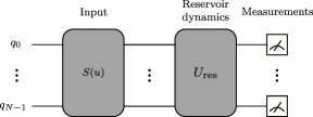
Figure 1: (a) Schematic figure illustrating the implementation of a QRC scheme on a gate-based quantum computer. Here $S(u)$ is a unitary encoding the input into the quantum state, but this unitary can also be exchanged by the state initialization (non-unitary) as shown in (b). $U_{\text{res}}$ represents the unitary time-evolution of the used quantum reservoir. This time evolution is linear in every case.

This whole QRC procedure natively translates into the language of quantum circuits. The states of the qubits in a quantum circuit are manipulated by unitary gate operations and measurements. So formally, the input encoding with qubit rotations and the time evolution operator can be written as unitary gate operations, as illustrated in Fig. 1. $S(u)$ is the unitary to encode the input into the qubits. This unitary can also be exchanged with a non-unitary block implementing the state initialization as given in Eq. (4), which is shown in Fig. 1 (b). $U_{\text{res}}$ dislpays the unitary reservoir dynamics given by the time evolution operator in Eq. (5).

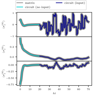
Figure 2: Qubit dynamics ($\sigma_{z}^{(i)}$ expectation values) of the TFIM with qubit dephasing calculated with matrices and simulated with a gate-based quantum circuit model. Cyan curve shows qubit dynamics only with the dephasing and blue curve shows dynamics under input injection.

To compare this circuit model with results obtained from the reservoir dynamics according to Eq. (8), we consider the $\sigma_{z}^{(i)}$ qubit dynamics of a three qubit TFIM. The system is initialized in a random state. Until time $ht=20$ the system evolves freely only being subject to the dephasing. From $ht=20$ onwards, a random input sequence $\{u_{k}\}_{k}$ is injected into the reservoir according to Eq. (4). Fig. 2 shows the results. Both approaches to the simulation of the TFIM yield identical qubit dynamics. This is only an example for the fact that any quantum system used as physical reservoir can equivalently be simulated on a programmable quantum computer. The main obstacle for practical implementation is the circuit depth of $U_{\text{res}}$ on actual quantum computing hardware. Quantum computers possess a set of native gate operations that all other unitary gates are decomposed into. As an example, we have decomposed the TFIM unitary time evolution corresponding to one time multiplexing step $\Delta_{t}/V$ into the native gate set of the IBM kyiv device [28]. The resulting circuit is displayed in Fig. 9 of App. A. Clearly, a circuit for simulation of multiple time steps exceeds the feasible number of gate operations on current NISQ hardware, which lies in the range of a few hundred gates [29].
We note that the difficulties of simulating physical reservoirs on a gate-based architecture does not neccessarily represent a drawback, since the idea of RC is to harness the internal dynamics of physical systems rather than programming it. Still, the connection of both computing platforms enables us to use quantum circuits as reservoirs to analyse general aspects of QRC. We will do this in the next section to give an upper bound for the expressivity of the QRC framework.

III Limits of expressivity given by the input encoding

Our main goal is to quantify the expressive power of the QRC framework. Therefore, we will use a measure which quantifies the expressivity in terms of the number of linearly independent functions a system can express. The expressivity depends on the way the input is injected into the dynamical system, as well as on the reservoir dynamics itself. We will investigate both dependencies and focus on the former in this section, while the latter will be covered in later sections.

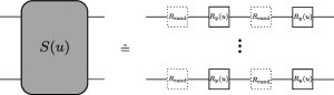
Figure 3: Illustration of the input injection with single qubit Pauli rotations. Before each input encoding, the quibts are randomly rotated.

The usual QRC procedure is displayed in Fig. 1. The system is initialized in a state, the first input is injected and then, the system evolves under the reservoir dynamics. This is followed by either the first measurement or by the next cycle of input injection and reservoir dynamics. So until the measurements are preformed, the state of the system is changed in two ways, either by the input encoding of by the unitary reservoir dynamics. Although the input encoding has the ability to inject the input in a non-linear way (e.g. by single qubit Pauli rotations) [30, 31], the unitary reservoir dynamics change the state’s dependence on the input only in a linear fashion. While the input to the system changes in every cycle, the reservoir dynamics stay the same. E.g. considering input $u_{i}$ of the $i$-th cycle, the reservoir cannot introduce a more complex dependency of the output features on the input $u_{i}$ with just passing through more cycles. Because of this, it is sufficient to consider only one cycle of the QRC scheme in order to assess the expressivity of a reservoir. This is reminiscent of an extreme learning machine (ELM) and, indeed, the procedure for analysing the expressivity is the same for ELMs and QRC.

Apart from this, we make three adaptions to our setup from section II. Firstly, we choose to suppress the influence of dephasing. This allows us to determine a theoretical upper bound for the maximum number of linearly independent functions the QRC framework can express. Secondly, from here on, we extract information from the reservoir by a positive operator-valued measure (POVM). We choose the $n$-th POVM element $M_{n}$ to be a zero matrix with 1 at the $n$-th position on the diagonal. This effectively measures all diagonal elements of the density matrix. Thirdly, we change the way the input is injected into the system according to Fig. 3. The input encoding consitst of gates of the form $\text{e}^{\text{i}uG}$, with an encoding Hamiltonian $G$. Each input layer is preceded by a layer of random single qubit rotations. We assume the encoding Hamiltonian $G$ to be diagonal. If $G$ is not diagonal, we can always diagonalize it ($\text{e}^{\text{i}uG}=\text{e}^{\text{i}uV\Sigma V^{*}}$) and absorb $V$ in the random rotations and $V^{*}$ either in $R_{\text{rand}}$ or in $U_{\text{res}}$.

A similar setup was used in Ref. [24], where the authors assumed a quantum model of the form

$$f_{\bm{\theta}}(u)=\Braket{0|U^{\dagger}(u,\bm{\theta})MU(u,\bm{\theta})|0}\quad,$$ (12)

with $U(u,\bm{\theta})$ representing the quantum circuit which depends on the input $u$ and some parameters $\bm{\theta}$. $M$ is an observable. In Ref. [24], Schuld and coworkers showed that this quantum model, given that the input is encoded by gates of the form $\text{e}^{\text{i}uG}$, is given by a partial Fourier series

$$f_{\bm{\theta}}(u)=\sum_{\omega\in\Omega}c_{\omega}(\bm{\theta})\text{e}^{\text{i}\omega u}\quad,$$ (13)

where the frequency spectrum $\Omega$ is solely determined by the eigenvalues of the encoding Hamiltonian $G$. Our QRC circuit resembles this setup except for the measurement. Instead of using a single observable, here, we use $N$ operators for the POVM measurement. Hence, we have a set of functions $\bm{f}_{\bm{\theta}}(u)=\{f_{\bm{\theta}}^{(n)}(u)\}_{n}$, which all have the same structure of a partial Fourier series:

$$f_{\bm{\theta}}^{(n)}(u)=\sum_{\omega\in\Omega}c_{\omega}^{(n)}(\bm{\theta})\text{e}^{\text{i}\omega u}\quad.$$ (14)

Using Pauli rotation gates for the encoding, Ref. [24] showed that the frequency spectrum $\Omega$ grows linearly with the number of input gates, i.e., $r$ repetitions of single qubit Pauli gates, either in parallel or sequentially, give rise to a truncated Fourier series of degree $r$. This means that the model represents a real Fourier series with $r$ distinct frequencies. So each output from our QRC model, as given in Eq. (14) is such a truncated Fourier series of degree $r$. Consequently, the upper bound of the maximum possible number of linearly independent functions the QRC can express is given by

$$C_{\text{T}}^{\text{max}}=2r+1\quad,$$ (15)

where $r$ is the number of Pauli rotations used for the input encoding. This simple formula carries an important meaning, namely that the expressivity of a QML approach cannot be improved by enlarging the Hilbert space of the underlying quantum-mechanical system.

We support this theoretical analysis with numerical simulations using the concept of the resolvable expressive capacity and eigentasks, introduced recently in Ref. [25]. Within this framework a quantum system is considered as an input-output map. Input $u\in\mathbb{R}$ is injected into the system and the output is obtained by a POVM, which measures $K$ degrees of freedom $X_{k}$. The experimental issue of shot noise is accounted for by introducing the average values of stochastic features $X_{k}^{(s)}$ under $S$ shots

$$\bar{X}_{k}(u)=\frac{1}{S}\sum_{s=1}^{S}X_{k}^{(s)}(u)\quad,$$ (16)

which allows one to calculate the resolvable expressive capacity (REC) $C_{\text{T}}$. The REC is a measure of the expressivity by quantifying how many linearly independent functions the system can express. These functions are called eigentasks and $C_{\text{T}}$ is the quantity for which we presented the upper bound in dependence of the input encoding in Eq. (15).

We support this finding by calculating the REC in dependence of the number of input encoding gates. We do this by neglecting measurement statistics (infinite shots) and extract the results of the POVM directly from the density matrix to facilitate a direct comparison with the theoretical upper bound. Furthermore, we compare the REC values of a product state possessing $U_{\text{res}}=\mathds{1}$ with a QRC model, where $U_{\text{res}}$ is an entangling ansatz. The task of finding a good entangling ansatz is recognised as a central design element of PQCs in QML [32, 33, 34]. Since our main focus is not the design of a suitable gate-based reservoir, we choose already existing circuits. For our analysis, we refrain from introducing arbitrary ansätze, but instead use the 19 different circuits that were introduced in Sim et al. [35], which are reprinted in Appendix B for convenience.

For the following investigations, it is worthwhile to stress the difference between expressibility and expressivity. The former refers to the circuit’s ability to explore the Hilbert space, i.e. how much of the Hilbert space can be covered by the circuit. The expressivity, on the other hand, is a measure of how many linearly independent functions can be expressed at the output of a dynamical system.

For the purpose of investigating the dependence of the expressivity on the input encoding, we consider an entangling ansatz that ideally produces a high expressivity, which is circuit 6 from Ref. [35] also displayed in Appendix B. The expressivity results of the product system and the one with this entangling ansatz are shown in Fig. 5.

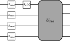
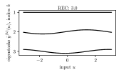
Figure 4: Left: Quantum circuit with a single input encoding gate using an entangling ansatz. Right: The corresponding eigentasks using circuit 6 in Fig. 10.

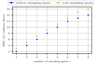
Figure 5: REC values for a quantum circuit in dependence of the number of input encoding gates. Results were obtained without shot noise (infinite shots).

The quantum circuit with a single-qubit encoding via a rotation gate has access to a single frequency as presented in Ref. [24], which leads to a simple sine function as eigentask. Furthermore, the circuit can express a function that is independent of the input, i.e. a constant. This results in a REC of two, as fulfilled by the product state. The same circuit with one rotational input gate and an additional entangling layer has still access to a single frequency. The entangling layer enables the ‘distribution’ of the input information to other degrees of freedom. In this way, the circuit can construct an additional orthogonal function of the same frequency, which in this case is the cosine that appears in Fig. 4. For every rotational input gate that is added, the accessible frequency spectrum is extended by one frequency, increasing the number of eigentasks by two if an an entangling layer is being used. Hence, the input-gate-number dependent upper bound (Eq. (15)) is perfectly replicated by our REC calculations shown in Fig. 5.

An exception to this is the case of using eight encoding gates for the input, where Eq. (15) predicts a value of $C_{\text{T}}=17$. The reason for this is that this the REC value is not only limited by the number of input gates, but also by the number of the measured degrees of freedom as elaborated in Ref. [25]. The number of measured degrees of freedom is 16 in our setup due to the POVM on four qubits, restricting the REC to the same value.

Fig. 5 also shows the expressivity in dependence of the number of input gates in product state systems. These systems feature a reduced expressivity, because the information is injected at the level of the individual qubits, in which case the output can only be composed as a superposition of an incomplete set of eigenvalues of the total many-particle system.

Reaching the upper bound in Eq. 15 is only possible if the entangling layer allows for the distribution of the input information into different degrees of freedom of the system. Consequently a layer of CNOT gates possesses the same REC value as the product state [25]. An important aspect that we have not yet considered is the presence of noise, which is always present in real-world implementations. Finite noise-to-signal ratios (NSRs) prevent reaching this upper bound, leading to the question, which ansatz circuits maximize the expressivity under such conditions. In the following two sections, we investigate the expressivity of systems where we use the time-evolution of the TFIM as reservoir in the presence of shot noise and compare it with different ansatz circuits.

IV Resolvable expressive capacity in QRC

Up to now, we used as reservoir $U_{\text{res}}$ only gate-based ansätze. Next, we apply the expressivity analysis to the field of physical QRC. Meaning that by using the methods from Section II, we exchange $U_{\text{res}}$ by the unitary time-dynamics of a physical quantum system, chosen to be the TFIM.

The setup we consider is the one depicted in Fig. 1, but for the input encoding, we now specify two different scenarios that are illustrated in Fig. 6.

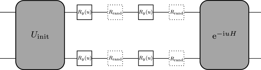
Figure 6: QRC scheme for determining the REC, where two cases are considered: First case is without the random rotations (symmetric system) and the second case includes the random rotations to break the symmetry.

In the first case, the input encoding layer is directly followed by $U_{\text{res}}$, i.e. the dynamics of the TFIM as given in Eq. 8. The second case adds a layer of random single qubit rotations after each input layer to break the symmetry. This layer has been shown to be beneficial, as the presence of symmetries in the system limits the attainable expressivity below its theoretical maximum [25]. Since in the TFIM all qubits are treated equally, our system possesses an intrinsic symmetry due to the Hamiltonian being not only Hermitian but also symmetric. In an experimental setup of the physical system, the breaking of symmetry might already occur due to the presence of noise of such an open quantum systen.

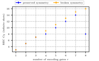
Figure 7: REC values of the TFIM in dependence of the input encoding.

The statistical nature of the quantum-measurement processes is not accounted for at this stage by assuming exact expectation values. We will explicitly consider the impact of the measurement statistics in Section V.

The REC that persists under these circumstances is shown in Fig. 7 in dependence on the number of input encodings. For the first three encoding gates, the QRC based on the TFIM behaves similarly to the quantum circuit with an entangling ansatz. No difference between the symmetric and the broken-symmetry system is observed, because the input is injected on only three out of four qubits, thereby destroying the underlying symmetry. However, adding a fourth encoding gate introduces a discrepancy between both systems, because the input is injected symmetrically on all qubits. Increasing the number of input gates further, it becomes apparent that the broken-symmetry system exhibits the maximal achievable REC values following our upper bound in Eq. 15, meaning that the time evolution of the TFIM is maximally expressive in a theoretical ideal and symmetry broken scenario. In a system with symmetries, the expressivity is reduced as already mentioned in Ref. [25]. In the extreme case of eight encoding gates, we find an attainable REC of $C_{\text{T}}=8$, caused on the one hand, by the symmetric Hamiltonian, and, on the other hand, also by the symmetric input encoding. One should point out that in an experimental realization, depending on the underlying hardware platform, perfectly symmetric systems will not likely be realized due to inhomogeneity and dissipation processes.

V Gate-based ansätze for a QRC scheme

In this section we aim for a more realistic calculation of the expressivity and consider the impact of shot noise when performing a finite number of measurements. This will generally reduce the REC due to the non-zero noise-to-signal ratios (NSRs) of the eigentasks. The NSRs depend on the underlying system, in particular on the used reservoir.

Although, the idea of RC is to use physical systems as reservoir implementation rather than programmable (quantum) computers, the gate-based approach offers an opportunity to investigate the general properties of quantum systems in RC. Furthermore, the gate-based architecture could offer a more approachable platform for RC in the NISQ era. Here, we analyse the use of the different ansatz circuits from Sim et al. [35] (refer to Fig. 10) as reservoirs.

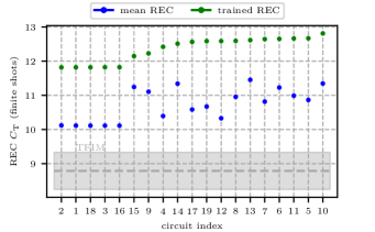
Figure 8: Blue: REC for different ansatz circuits. Values are calculated by randomly sampling circuits parameters and averaging over 200 realizations. Green: REC values of the circuits with optimized, rather than randomly sampled, parameters. Parameters of the ansatz circuits have been optimized for a maximal expressivity. Dashed gray line indicates the expressivity of the non-optimized TFIM optimized over 50 reservoir realizations. Shaded gray area indicates the standard deviation.

The REC values for all considered circuits are shown in Fig. 8. As expected, a product state, as realized by circuit 1, has the lowest expressivity. Circuit 2, which produces an entangled state via a single layer of CNOT gates, possesses the same expressivity. Again, this shows that entanglement alone is not the reason for a circuit to be expressive. Circuits 3, 16 and 18 also have a low expressivity, which could be explained by the fact that, in these circuits, the controlled rotations address the same degrees of freedom as the single qubit rotations prior to them. Apart from that, the circuits 13 and 14 with controlled rotations perform quite well in general. For the expressivity, it seems to be beneficial if ansatz circuits have alternating parts between entangling gates and single-qubit rotations. Especially circuit 15, which uses solely CNOT gates for entanglement generation, shows large improvement compared to circuit 3. Also the high-depth circuits 5 and 6, in which entangling gates and single-qubit rotations are not mixed, perform worse than circuits 13 and 14.

The shown results demonstrate that, in contrast to classical reservoirs and possibly against intuition, QRCs get their expressivity not from the reservoir. Once, the reservoir introduces sufficient complexity for achieving maximal expressivity as allowed due to the input encoding, further increasing the size of the reservoir or its complexity cannot improve the expressivity. The expressivity is primarily determined by two factors: firstly by the way the input is injected as shown here, and secondly by the number of readouts that are preformed [25]. The reservoir can only change the number of functions that are accessible, but the source for expressivity lies in the input injection. To be precise, the set of non-linear orthogonal functions the reservoir has access to is independent of the reservoir, since the time evolution in quantum mechanics is inherently linear. Non-linearity can only be introduced by the encoding gates.

Before concluding, we address the expressivity of the physical QRC that is also shown in Fig. 8. Interestingly, the TFIM has the lowest REC value among all tested reservoirs, performing even worse than the product-state circuit. We attribute this result to the specific dynamics produced by the time evolution of the TFIM, leading to output functions with high NSRs, thus lowering the expressivity. Besides the higher expressivity of the ansatz circuits, the gate-based approach to QRC has the additional advantage over pyhsical reservoirs that their parameters can be precisely tuned and, therefore, be used for optimization. To do so, we employ an approach similar to parameterized quantum circuits in QML by performing an optimization step of the parameters of all ansatz circuits shown in Fig. 10 to maximize the attainable expressivity. The REC values for the optimized circuits are shown in green in Fig. 8. The results indicate that this approach generally improves the performance, although the increase in expressivity varies significantly among the individual quantum circuits. While the REC values of the worst performing circuits get a large increase after optimization, circuits 14 and 15 improve only slightly. Generally, after optimization there are less differences in the performance of the quantum circuits indicating that optimization is worthwhile in any case.

An open question remains how the noise-to-signal ratios of the eigentasks are affected by the specific choice of the circuit, which will be the topic of future investigations.

VI Conclusion

The central conclusion of our work is the counter-intuitive fact that in physical reservoir computing, there is a fundamental difference between classical and quantum hardware platforms: While classical RC draws its capabilities from the complex non-linear dynamics that is inherent to the reservoir, the size and connectivity of a quantum reservoir does not determine its expressivity, which serves as a measure for the complexity of the output that can be generated from the input data.

To reveal this fact, we have translated the QRC approach into the language of circuit-based QML, establishing a fundamental connection on an abstract level between these two very different QML paradigms. This analogy enables one to compare the expressivity of the TFIM as a representative for a physical QRC with a selection of different gate-based low-depth ansatz circuits. We find all of these ansatz circuits to outperform the TFIM with the additional benefit that they can be optimized via their parametrization, which is generally not possible in a physical reservoir. We explicitly show that the upper bound for the number of linear independent functions a reservoir can express is limited by the number of input encoding gates. Considering the inherent linearity of quantum mechanics, it is impossible to increase the available number of linear independent functions by increasing the complexity or the size of the quantum reservoir. In other words, the available function space is solely determined by the number of input encoding gates, while the reservoir topology merely influences the number of orthogonal functions that are accessible.

The insight we provide carries an important message into the field of physical QML and QRC, namely that the exponentially large state space one finds in quantum mechanics cannot be used as an advantage of quantum over classical RC. Harnessing this quantum advantage requires the input encoding to address the available degrees of freedom that, otherweise, remain unaccessible for computing. While this problem could be mitigated at the input-encoding stage, doing so will require precise control over the input encoding, which is generally not the idea behind physical QRC and is further limited by the NISQ hardware that is currently available.

Acknowledgements

The authors would like to thank Frederik Lohof for many useful discussions. This work has been supported by the Quantum Computing Initiative of the DLR via the Quantum Fellowship Programme. We also acknowledge funding from the German Research Foundation (DFG) via the project Gi1121/6-1.

Appendix A Transpilation of the time-evolution of the TFIM

Simulation of the TFIM on a gate-based quantum computer requires a transpilation of the unitary time-evolution of the Ising system into the native gate set of the used quantum computer. As example, we transpiled the time-evolution operator, as given by Eq. (5), into the native gate-set of the IBM kyiv device. We performed the transpilation for a single multiplexing step of $\Delta_{t}/V$. The transpiled circuit is shown in Fig. 9.

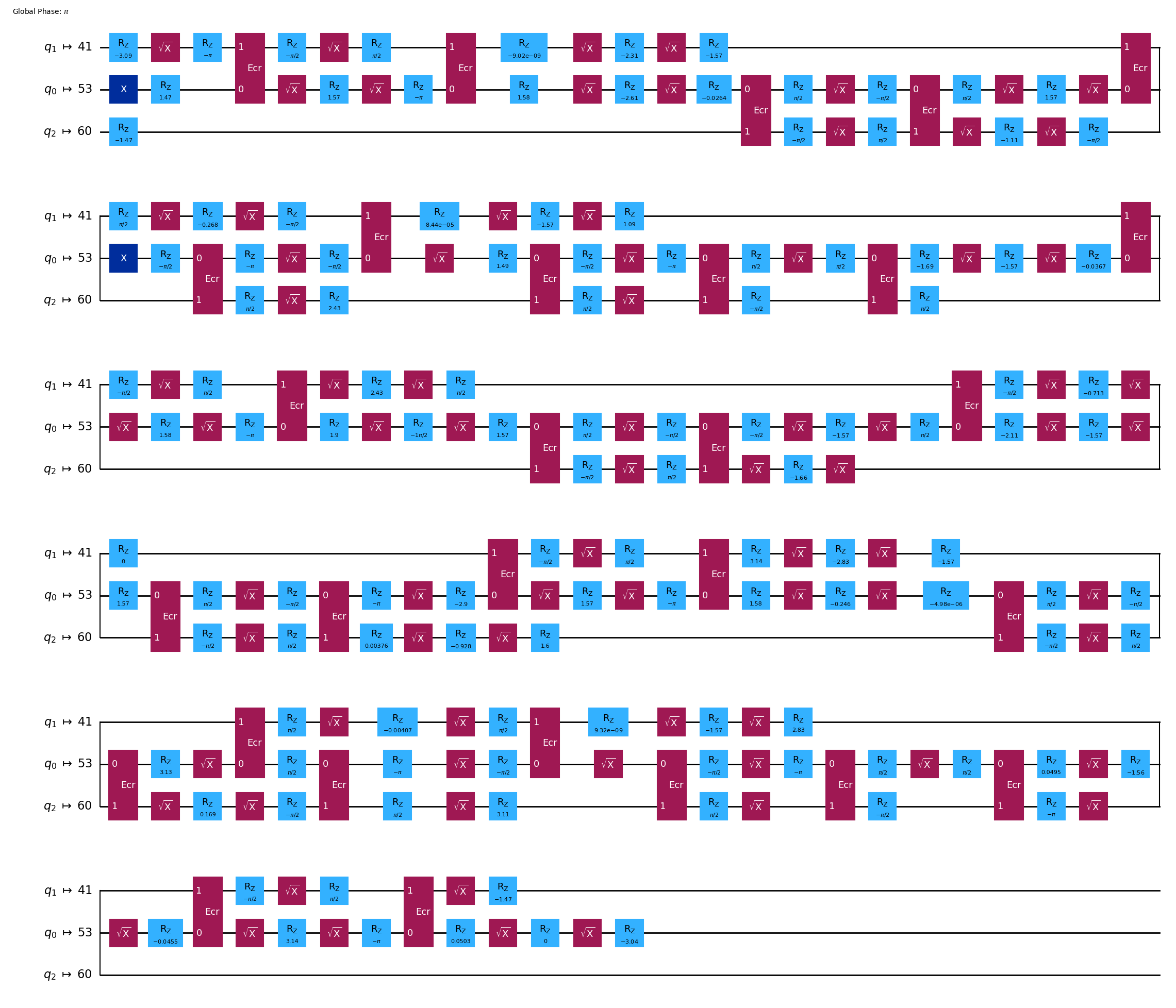
Figure 9: Transpiled circuit of the unitary which implements one time-multiplexing step of the TFIM. Transpilation was done with respect to the native gate set of the ibm kyiv device.

Appendix B Ansatz circuits

For convenience, we show the ansatz circuits used by Sim et al. [35] in Fig. 10.

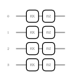
Circuit 1

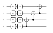
Circuit 2

Circuit 3

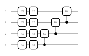
Circuit 4

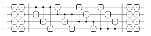
Circuit 5

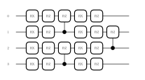
Circuit 7

Circuit 6

Circuit 8

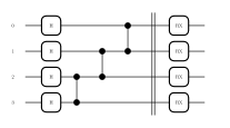
Circuit 9

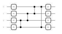
Circuit 10

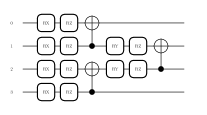
Circuit 11

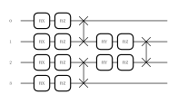
Circuit 12

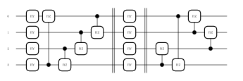
Circuit 13

Circuit 14

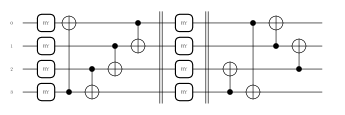
Circuit 15

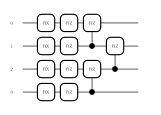
Circuit 16

Circuit 17

Circuit 18

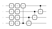
Circuit 19

Figure 10: Ansatz circuits that are considered in the main text. The circuits are given in the same order as in [35] for better comparability.

References

- Shor [1994] P. Shor, Algorithms for quantum computation: Discrete logarithms and factoring, in Proceedings 35th Annual Symposium on Foundations of Computer Science (IEEE Comput. Soc. Press, Santa Fe, NM, USA, 1994) pp. 124–134.
- Shor [1997] P. W. Shor, Polynomial-Time Algorithms for Prime Factorization and Discrete Logarithms on a Quantum Computer, SIAM Journal on Computing 26, 1484 (1997).
- Grover [1996] L. K. Grover, A fast quantum mechanical algorithm for database search, in Proceedings of the Twenty-Eighth Annual ACM Symposium on Theory of Computing - STOC ’96 (ACM Press, Philadelphia, Pennsylvania, United States, 1996) pp. 212–219.
- Mitarai et al. [2018] K. Mitarai, M. Negoro, M. Kitagawa, and K. Fujii, Quantum circuit learning, Physical Review A 98, 032309 (2018).
- Schuld and Killoran [2019] M. Schuld and N. Killoran, Quantum Machine Learning in Feature Hilbert Spaces, Physical Review Letters 122, 040504 (2019).
- Havlíček et al. [2019] V. Havlíček, A. D. Córcoles, K. Temme, A. W. Harrow, A. Kandala, J. M. Chow, and J. M. Gambetta, Supervised learning with quantum-enhanced feature spaces, Nature 567, 209 (2019).
- Fujii and Nakajima [2017] K. Fujii and K. Nakajima, Harnessing Disordered-Ensemble Quantum Dynamics for Machine Learning, Physical Review Applied 8, 024030 (2017).
- Nakajima et al. [2019] K. Nakajima, K. Fujii, M. Negoro, K. Mitarai, and M. Kitagawa, Boosting Computational Power through Spatial Multiplexing in Quantum Reservoir Computing, Physical Review Applied 11, 034021 (2019).
- Čindrak et al. [2024a] S. Čindrak, B. Donvil, K. Lüdge, and L. Jaurigue, Enhancing the performance of quantum reservoir computing and solving the time-complexity problem by artificial memory restriction, Physical Review Research 6, 013051 (2024a).
- Dudas et al. [2023] J. Dudas, B. Carles, E. Plouet, F. A. Mizrahi, J. Grollier, and D. Marković, Quantum reservoir computing implementation on coherently coupled quantum oscillators, npj Quantum Information 9, 64 (2023).
- Mujal et al. [2023] P. Mujal, R. Martínez-Peña, G. L. Giorgi, M. C. Soriano, and R. Zambrini, Time-series quantum reservoir computing with weak and projective measurements, npj Quantum Information 9, 16 (2023).
- Suzuki et al. [2022] Y. Suzuki, Q. Gao, K. C. Pradel, K. Yasuoka, and N. Yamamoto, Natural quantum reservoir computing for temporal information processing, Scientific Reports 12, 1353 (2022).
- Govia et al. [2021] L. C. G. Govia, G. J. Ribeill, G. E. Rowlands, H. K. Krovi, and T. A. Ohki, Quantum reservoir computing with a single nonlinear oscillator, Physical Review Research 3, 013077 (2021).
- Llodrà et al. [2023] G. Llodrà, C. Charalambous, G. L. Giorgi, and R. Zambrini, Benchmarking the Role of Particle Statistics in Quantum Reservoir Computing, Advanced Quantum Technologies 6, 2200100 (2023).
- Götting et al. [2023] N. Götting, F. Lohof, and C. Gies, Exploring quantumness in quantum reservoir computing, Physical Review A 108, 052427 (2023).
- Čindrak et al. [2024b] S. Čindrak, L. Jaurigue, and K. Lüdge, Krylov Expressivity in Quantum Reservoir Computing and Quantum Extreme Learning (2024b), arXiv:2409.12079 [quant-ph] .
- Olivera-Atencio et al. [2023] M. L. Olivera-Atencio, L. Lamata, and J. Casado-Pascual, Benefits of Open Quantum Systems for Quantum Machine Learning, Advanced Quantum Technologies , 2300247 (2023).
- Sannia et al. [2024] A. Sannia, R. Martínez-Peña, M. C. Soriano, G. L. Giorgi, and R. Zambrini, Dissipation as a resource for Quantum Reservoir Computing, Quantum 8, 1291 (2024), arXiv:2212.12078 [quant-ph] .
- Kora et al. [2024] Y. Kora, H. Zadeh-Haghighi, T. C. Stewart, K. Heshami, and C. Simon, Frequency- and dissipation-dependent entanglement advantage in spin-network Quantum Reservoir Computing (2024), arXiv:2403.08998 [quant-ph] .
- Martínez-Peña et al. [2021] R. Martínez-Peña, G. L. Giorgi, J. Nokkala, M. C. Soriano, and R. Zambrini, Dynamical Phase Transitions in Quantum Reservoir Computing, Physical Review Letters 127, 100502 (2021).
- Palacios et al. [2024] A. Palacios, R. Martínez-Peña, M. C. Soriano, G. L. Giorgi, and R. Zambrini, Role of coherence in many-body Quantum Reservoir Computing, Communications Physics 7, 369 (2024).
- Jaeger [2001] H. Jaeger, Short Term Memory in Echo State Networks, Technical report (GMD-Forschungszentrum Informationstechnik (2001).
- Kobayashi et al. [2024] K. Kobayashi, K. Fujii, and N. Yamamoto, Feedback-Driven Quantum Reservoir Computing for Time-Series Analysis, PRX Quantum 5, 040325 (2024).
- Schuld et al. [2021] M. Schuld, R. Sweke, and J. J. Meyer, Effect of data encoding on the expressive power of variational quantum-machine-learning models, Physical Review A 103, 032430 (2021).
- Hu et al. [2023] F. Hu, G. Angelatos, S. A. Khan, M. Vives, E. Türeci, L. Bello, G. E. Rowlands, G. J. Ribeill, and H. E. Türeci, Tackling Sampling Noise in Physical Systems for Machine Learning Applications: Fundamental Limits and Eigentasks, Physical Review X 13, 041020 (2023).
- Stinchcombe [1973] R. B. Stinchcombe, Ising model in a transverse field. I. Basic theory, Journal of Physics C: Solid State Physics 6, 2459 (1973).
- Pfeuty and Elliott [1971] P. Pfeuty and R. J. Elliott, The Ising model with a transverse field. II. Ground state properties, Journal of Physics C: Solid State Physics 4, 2370 (1971).
- 202 [2025] IBM kyiv, https://quantum.ibm.com/services/resources?resourceType=current-instance&system=ibm_kyiv (2025).
- Lau et al. [2022] J. W. Z. Lau, K. H. Lim, H. Shrotriya, and L. C. Kwek, NISQ computing: Where are we and where do we go?, AAPPS Bulletin 32, 27 (2022).
- Mujal et al. [2021] P. Mujal, J. Nokkala, R. Martínez-Peña, G. L. Giorgi, M. C. Soriano, and R. Zambrini, Analytical evidence of nonlinearity in qubits and continuous-variable quantum reservoir computing, Journal of Physics: Complexity 2, 045008 (2021).
- Govia et al. [2022] L. C. G. Govia, G. J. Ribeill, G. E. Rowlands, and T. A. Ohki, Nonlinear input transformations are ubiquitous in quantum reservoir computing, Neuromorphic Computing and Engineering 2, 014008 (2022).
- Benedetti et al. [2019] M. Benedetti, E. Lloyd, S. Sack, and M. Fiorentini, Parameterized quantum circuits as machine learning models, Quantum Science and Technology 4, 043001 (2019), arXiv:1906.07682 [quant-ph] .
- Du et al. [2022] Y. Du, T. Huang, S. You, M.-H. Hsieh, and D. Tao, Quantum circuit architecture search for variational quantum algorithms, npj Quantum Information 8, 62 (2022).
- Pirhooshyaran and Terlaky [2021] M. Pirhooshyaran and T. Terlaky, Quantum circuit design search, Quantum Machine Intelligence 3, 25 (2021).
- Sim et al. [2019] S. Sim, P. D. Johnson, and A. Aspuru-Guzik, Expressibility and Entangling Capability of Parameterized Quantum Circuits for Hybrid Quantum-Classical Algorithms, Advanced Quantum Technologies 2, 1900070 (2019).