Uniform-in-time propagation of chaos for the Cucker–Smale model

Abstract

This paper presents an elementary proof of quantitative uniform-in-time propagation of chaos for the Cucker–Smale model under sufficiently strong interaction. The idea is to combine existing finite-time propagation of chaos estimates with existing uniform-in-time stability estimates for the interacting particle system, in order to obtain a uniform-in-time propagation of chaos estimate with an explicit rate of convergence in the number of particles. This is achieved via a method that is similar in spirit to the classical “stability + consistency implies convergence” approach in numerical analysis.

1 Introduction

Let $\bigl{(}x^{j}_{0},v^{j}_{0}\bigr{)}_{j\in\mathbf{N}}$ denote independent random variables with common distribution $\overline{\rho}_{0}\in\mathcal{P}(\real^{d}\times\real^{d})$. We consider for $J\in\mathbf{N}$ the following interacting particle system as in [22]:

$$\left\{\begin{aligned} \mathrm{d}X^{j}_{t}&=V^{j}_{t}\,\mathrm{d}t,\\ \mathrm{d}V^{j}_{t}&=-\frac{K}{J}\sum_{k=1}^{J}\psi\Bigl{(}\bigl{\lvert}X^{j}_{t}-X^{k}_{t}\bigr{\rvert}\Bigr{)}\left(V^{j}_{t}-V^{k}_{t}\right)\,\mathrm{d}t,\end{aligned}\right.\qquad\left(X^{j}_{0},V^{j}_{0}\right)=\left(x^{j}_{0},v^{j}_{0}\right)\stackrel{{\scriptstyle\rm i.i.d.}}{{\sim}}\overline{\rho}_{0}.$$ (1.1)

Here $K$ denotes the communication strength, and $\psi\colon(0,\infty)\to(0,\infty)$ is a globally Lispchitz continuous, non-increasing function that is bounded from above by 1. That is to say:

$$\psi>0,\qquad\left\lVert\psi\right\rVert_{L^{\infty}}\leqslant 1,\qquad\left\lVert\psi\right\rVert_{\rm Lip}<\infty,\qquad\bigl{(}\psi(r_{1})-\psi(r_{2})\bigr{)}(r_{1}-r_{2})\leqslant 0\quad\forall r_{1},r_{2}>0.$$ (1.2)

This is a standing assumption throughout this paper. An example given in [3] of a function satisfying these assumptions is $\psi(z)=\left(1+z^{2}\right)^{-\gamma},$ for some $\gamma\geqslant 0$. Equation (1.1) is known as the Cucker–Smale dynamics [11, 9], a widely studied model to describe the evolution of flocks. Propagation of chaos for (1.1) refers to the property that, in the limit as $J\to\infty$ in (1.1), each particle behaves independently of any other individual particle, with a law equal to that of the nonlinear Markov process that solves the following McKean–Vlasov equation:

$$\left\{\begin{aligned} \mathrm{d}\overline{X}_{t}&=\overline{V}_{t}\,\mathrm{d}t\\ \mathrm{d}\overline{V}_{t}&=-K\left(H\star\overline{\rho}_{t}\right)\left(\overline{X}_{t},\overline{V}_{t}\right)\,\mathrm{d}t,\qquad\qquad\left(\overline{X}_{0},\overline{V}_{0}\right)\sim\overline{\rho}_{0},\\ \overline{\rho}_{t}&={\rm Law}(\overline{X}_{t},\overline{V}_{t}),\end{aligned}\right.$$ (1.3)

where $H(x,v)=\psi(\lvert x\rvert)v$ and the convolution between $H\colon\real^{d}\times\real^{d}\to\real^{d}$ and $\mu\in\mathcal{P}(\real^{d}\times\real^{d})$ is defined as

$$(H\star\mu)(x,v)=\iint_{\real{}^{d}\times\real^{d}}H(x-y,v-w)\,\mu(\mathrm{d}y\,\mathrm{d}w).$$

The dynamics of the mean field law $(\overline{\rho}_{t})_{t\geqslant 0}$ is governed by the following McKean–Vlasov equation:

$$\partial_{t}\overline{\rho}_{t}+v\cdot\nabla_{x}\overline{\rho}_{t}-K\nabla_{v}\cdot\bigl{(}H\star\overline{\rho}_{t}\bigr{)}=0,\qquad x,v\in\real^{d}.$$ (1.4)

The existence of a globally defined measure valued solution to this equation is proved in [23, Section 6]. As noted in Remark 5.1 of that reference, see also [22, Remark 8], the empirical measure associated to any solution of the interacting particle system (1.1) is itself a measure-valued solution to (1.4).

In this short paper we prove that, given a uniform-in-time stability estimate for the interacting particle system (1.1) and a decay estimate for the nonlinear process (1.3), quantitative uniform-in-time propagation of chaos easily follows. We present this approach for the particular case of the Cucker–Smale model, but note that this strategy can be applied more generally. It would be interesting, for example, to investigate whether a similar analysis can be carried out for optimization methods based on interacting particle systems, such as ensemble Kalman inversion [26, 2, 1] and recently proposed methods based on consensus formation [36, 5, 16]. Local-in-time propagation of chaos estimates for these systems are proved in [12, 13, 38] and [25, 18, 27], respectively.

We emphasize that, in contrast with the classical reference [23] on the mean field limit for the Cucker–Smale dynamics, where initial configurations for (1.1) supported on a regular lattice are considered in order to understand the convergence of the particle-in-cell method for solving the nonlinear equation (1.4), we consider only the setting where the particles forming the initial configuration are randomly distributed in an independent, identically distributed (i.i.d.) manner, with common law $\overline{\rho}_{0}$. This setting was studied in [3], and the interacting particle system (1.1) with this initial condition may be viewed as an alternative, Monte Carlo-type approach to approximate the mean field dynamics, which is better suited to high-dimensional problems. To motivate the results we present, we consider the following natural questions concerning the relation between (1.1) and (1.3):

Question 1.

Suppose that the interacting particle system (1.1) with $J$ particles is employed to approximate the solution to the nonlinear process (1.3). Is it possible to prove, for some $\alpha>0$, a uniform-in-time error estimate for the Euclidean Wasserstein distance of the form

$$\sup_{t\geqslant 0}\Bigl{(}\mathbf{E}W_{2}\bigl{(}\mu_{\mathcal{Z}^{J}_{t}},\overline{\rho}_{t}\bigr{)}^{2}\Bigr{)}^{\frac{1}{2}}\lesssim J^{-\alpha}\,?\qquad\mu_{\mathcal{Z}^{J}_{t}}:=\frac{1}{J}\sum_{j=1}^{J}\delta_{\bigl{(}X^{j}_{t},V^{j}_{t}\bigr{)}}.$$ (1.5)

Question 2.

The distance used in estimate (1.5) is of course not the only metric to compare the interacting particle system with the nonlinear process (1.3). It is also of interest to prove, for some $\beta>0$, a uniform-in-time error estimate of the form

$$\sup_{t\geqslant 0}W_{2}\bigl{(}\rho^{J}_{t},\overline{\rho}^{\otimes J}_{t}\bigr{)}\lesssim J^{\frac{1}{2}-\beta}.$$ (1.6)

Here $\rho^{J}_{t}\in\mathcal{P}(\real^{2dJ})$ denotes the law of the solution to the interacting particle system (1.1), and $\overline{\rho}_{t}^{\otimes J}$ denotes the probability measure in $\mathcal{P}(\real^{2dJ})$ obtained by $J$-fold product the mean field law $\overline{\rho}_{t}$. The notation $W_{2}$ refers to the standard Euclidean Wasserstein distance, without the normalization as in [7, Definition 3.5].

Question 3.

Can the variance under the empirical measure $\mu_{\mathcal{Z}^{J}_{t}}$ be related to the variance under the law of the nonlinear process? More generally, given a test function $\varphi\colon\real^{2d}\to\real$, can a uniform-in-time error estimate of the following form be proved for some $\gamma>0$?

$$\sup_{t\geqslant 0}\left(\mathbf{E}\left\lvert\int_{\real{}^{2d}}\varphi(z)\,\mu_{\mathcal{Z}^{J}_{t}}(\mathrm{d}z)-\int_{\real{}^{2d}}\varphi(z)\,\overline{\rho}_{t}(\mathrm{d}z)\right\rvert^{2}\right)^{\frac{1}{2}}\lesssim J^{-\gamma}\,?$$ (1.7)

Weak convergence estimates of this form can be derived either from the estimate in ˜1, with rate $\gamma=\alpha$, or from an estimate of the type considered in ˜2, with a usually better rate $\gamma=\beta$. For a derivation of weak convergence results of type (1.7) from estimates of the form (1.6), we refer for example [13, Theorem 2] or [38, Corollary 5]; see also [31, Section 1] for related results.

To avoid any confusion, let us emphasize that, as stated, none of these estimates hold true for the Cucker–Smale interacting particle system with chaotic initial condition (1.1). They can be proved to hold, however, if all probability measures are recentred around their barycenter, as we shall explain in the next sections. To keep the discussion light, we do not worry about this point in this introduction.

Having already ˜3 is related to ˜1 and ˜2, we focus henceforth on the first two questions. In the terminology of [7, 8], the estimate (1.5) is a form of empirical chaos estimate, while (1.6) is an infinite-dimensional Wasserstein chaos estimate. Both estimates are of independent interest, and usually, the exponent $\alpha$ in (1.5) is smaller than the exponent $\beta$ in (1.6).

By the celebrated results in [17] on the Wasserstein distance between empirical measures formed from i.i.d. particles and the associated probability measure, estimate (1.5) follows from (1.6), with a constant $\alpha$ depending on $\beta$. However, in this note we shall first prove (1.5), and only then focus on (1.6), the reason being that empirical chaos is very simple to prove for (1.1) given existing results in the literature. Let us note, however, that the approach we take in Subsection˜4.1 for proving empirical chaos works only for interacting particle system which, apart from the initial condition, are deterministic, while the method of proof for (1.6) presented in Subsection˜4.2 does not rely on the deterministic nature of the evolution (1.1).

Contributions and organization of the paper

The main results of this paper are uniform-in-time estimates of the forms (1.5) and (1.6). These are presented in Subsections˜4.1 and 4.2, respectively, after a short literature review in Section˜2 and a presentation of auxiliary results in Section˜3. These auxiliary results, which are only stated in Section˜3 and proved in Section˜5, include a variant of the local-in-time propagation of chaos estimate from [3], as well as an extension of the uniform stability estimate for the particle system (1.1) proved in [22]. Finally, in Section˜6, we illustrate numerically the content of the main result of Subsection˜4.2.

Notation

To conclude this section, we introduce useful notation used throughout the remainder of this work. For solutions to the particle system (1.1), we use the notation

$$\mathcal{D}_{X}(t)=\max_{1\leqslant j,k\leqslant J}\lvert X^{j}_{t}-X^{k}_{t}\rvert,\qquad\mathcal{D}_{V}(t)=\max_{1\leqslant j,k\leqslant J}\lvert V^{j}_{t}-V^{k}_{t}\rvert$$ (1.8)

to denote the diameters in position and velocity space, respectively. Similarly, for the mean field law $\overline{\rho}_{t}$ we use the notation

$$\overline{\mathcal{D}}_{X}(t)=\max_{x,y\in\operatorname{supp}_{x}(\overline{\rho}_{t})}\lvert x-y\rvert,\qquad\overline{\mathcal{D}}_{V}(t)=\max_{v,w\in\operatorname{supp}_{v}(\overline{\rho}_{t})}\lvert v-w\rvert.$$ (1.9)

We also denote for conciseness $\Psi(x)=\psi(|x|)$ for $x\in\real^{d}$.

2 Literature review

Local-in-time propagation of chaos for the Cucker–Smale dynamics

Even for a finite time interval, proving propagation of chaos for (1.1) requires bespoke techniques, because the interaction is not globally Lipschitz continuous. The first result in this direction was obtained in [23], where a quantitative local-in-time mean field result is obtained for a compactly supported initial law $\overline{\rho}_{0}$. More precisely, the authors study the convergence with respect to $h$ of a deterministic particle method for solving the nonlinear equation (1.4), based on an approximation of the initial distribution $\overline{\rho}_{0}$ by an appropriate empirical measure over a lattice of size $h$.

Shortly after, [3] [3] proved a quantitative local-in-time propagation of chaos estimate, assuming chaotic initial data and strong control of the moments of the velocity marginal of $\overline{\rho}_{0}$. The technique presented there is a rather general strategy, summarized in [8, Section 3.1.2], which enables to prove quantitative propagation of chaos estimates for a wide class of models with only locally Lispchitz interactions, at the cost of very strong moment bounds on the solution to the nonlinear Markov process associated with the interacting particle system. The authors of [3] also prove global existence and uniqueness results for the interacting particle system (1.1) and the nonlinear process (1.3), again under strong moment bounds on the initial law $\overline{\rho}_{0}$.

The local-in-time mean field limit for the Cucker–Smale model is revisited later in [34], where the authors use an analytic rather than probabilistic coupling argument (which however appears equivalent to a probabilistic argument à la Sznitman), to obtain quantitative propagation of chaos estimates for a generalized Cucker–Smale dynamics, assuming that $\overline{\rho}_{0}$ is compactly supported.

Uniform-in-time mean field limit for the Cucker–Smale dynamics

The first results concerning the uniform-in-time mean field limit for (1.1) came from [22]. The type of results proved in this reference are of the following form: if a sequence of empirical measures $\mu_{\mathcal{Z}^{J}_{0}}=\frac{1}{J}\sum_{j=1}^{J}\delta_{(X^{j}_{0},V^{j}_{0})}\in\mathcal{P}(\real^{2d})$ converges to $\overline{\rho}_{0}$ in the Wasserstein-$p$ distance, then under appropriate conditions

$$\lim_{J\to\infty}\sup_{t\geqslant 0}W_{2}(\mu_{\mathcal{Z}^{J}_{t}},\overline{\rho}_{t})=0,$$ (2.1)

where $\mu_{\mathcal{Z}^{J}_{t}}$ is the empirical measure associated with the solution to (1.1) at time $t$. The proof of this result relies crucially on a uniform-in-time stability estimate for the interacting particle system (1.1), and it employs an argument to reinterpret solutions to (1.1) with different system sizes $J_{1}$ and $J_{2}$ as solutions with the same number of particles $J^{+}\geqslant\max\{J_{1},J_{2}\}$. The number $J^{+}$ can be taken as the least common multiple between $J_{1}$ and $J_{2}$. This trick is possible because, the evolution (1.1) being deterministic, the empirical measure associated with the solution at time $t$ depends only on the empirical measure at time 0, and not on the number or ordering of particles. That is to say, denoting by $(\mathcal{Z}^{J}_{t})$ and $(\widetilde{\mathcal{Z}}^{nJ}_{t})$ two solutions of (1.1) with respectively $J$ and $nJ$ particles, we have

$$\mu_{\mathcal{Z}^{J}_{0}}=\mu_{\widetilde{\mathcal{Z}}^{nJ}_{0}}\quad\Rightarrow\quad\mu_{\mathcal{Z}^{J}_{t}}=\mu_{\widetilde{\mathcal{Z}}^{nJ}_{t}},\qquad\text{for all $t\geqslant 0$}.$$

Let us emphasize that the result (2.1) from [22] holds only under certain assumptions. Notably, it is necessary that $\langle\mu_{\mathcal{Z}^{J}_{0}},\mathcal{V}\rangle=\langle\overline{\rho}_{0},\mathcal{V}\rangle$ for all sufficiently large $J$ and where $\mathcal{V}(x,v)=v$; that is, the mean velocity under the empirical measure must coincide with the mean velocity under the mean field law, eventually for large $J$. Indeed, if $\mu_{\mathcal{Z}^{J}_{0}}$ is an empirical measure such that $\langle\mu_{\mathcal{Z}^{J}_{0}},\mathcal{V}\rangle\neq\langle\overline{\rho}_{0},\mathcal{V}\rangle$, then the supremum in (2.1) is necessarily $+\infty$, as in this case the interacting particle system and the mean field solution $\overline{\rho}_{t}$ eventually drift away from each other. This is because (1.1) and (1.3) satisfy the following properties, which are simple to prove [23, Section 2]:

$$\frac{1}{J}\sum_{j=1}^{J}X^{j}_{t}=\frac{1}{J}\sum_{j=1}^{J}X^{j}_{0}+\left(\frac{1}{J}\sum_{j=1}^{J}V^{j}_{0}\right)t,\qquad\mathbf{E}\bigl{[}\overline{X}_{t}\bigr{]}=\mathbf{E}\bigl{[}\overline{X}_{0}\bigr{]}+\mathbf{E}\bigl{[}\overline{V}_{0}\bigr{]}t.$$

Furthermore, the result (2.1) is proved in an interaction regime where flocking is known to occur exponentially fast for the interacting particle system (1.1), i.e. in a regime where the velocities of all agents in (1.1) eventually coincide, both in direction and magnitude. Mathematically, a sufficient condition for exponential flocking for model (1.1) is that the initial law $\overline{\rho}_{0}$ is compactly supported in both space and velocity, and that the interaction strength $K$ is sufficiently large:

$$K>\frac{\overline{\mathcal{D}}_{V}(0)}{\int_{\overline{\mathcal{D}}_{X}(0)}^{\infty}\psi(s)\,\mathrm{d}s},$$ (2.2)

where we use the convention $\frac{1}{\infty}:=0$ in case the integral equals $+\infty$. Here and throughout this work, $B(x,r)$ denotes the ball of radius $r$ centered at $x$, so that $\frac{1}{2}B(x,d)$ is the ball of diameter $d$ centered at $x$ and $\overline{\mathcal{D}}_{X}(0)$ and $\overline{\mathcal{D}}_{V}(0)$ are defined in (1.9). For consistency with the notation in [22], we work with diameters $\overline{\mathcal{D}}_{X}$ and $\overline{\mathcal{D}}_{V}$ instead of the corresponding radii. The validity of a uniform-in-time mean field estimate in the setting of exponential flocking is not surprising, since the system practically stops moving after a finite time, relatively to its (usually time-dependent) space barycenter. There are many references on flocking for the Cucker–Smale dynamics, and we mention for example [24, 6], in addition to the references [23, 22] already mentioned.

Recent developments on uniform-in-time propagation of chaos for various models

To conclude this section, let us mention a few of the milestones among the flurry of advances concerning uniform-in-time mean field limits in recent years. We refer to [8, Section 3] for a more comprehensive overview. In [31], uniform-in-time propagation of chaos is proved for a gradient system in a convex potential via a synchronous coupling approach, and this result is used to prove exponentially fast convergence of the associated nonlinear process. The idea is extended to a class of kinetic dynamics, which however does not include the Cucker–Smale model, in [4]. Further extensions and generalizations were obtained in [32, 21]

In [14], a new technique based on reflection couplings is employed to relax convexity assumptions in uniform-in-time propagation-of-chaos results for gradient systems, and this technique is later adapted to the kinetic setting in [20]. Let us finally mention the work of Lacker [28], later adapted in [29] to the uniform-in-time setting, where a novel approach based on the BBGKY hierarchy is deployed to obtain for a class of interacting particle systems that an appropriate distance between the marginal law on the first $k$ particles of the interacting system on one hand, and the $k$-fold product of the mean field law on the other hand, scales as $\left(\frac{k}{N}\right)^{2}$, where previous arguments would only give a scaling as $\frac{k}{N}$.

Let us also mention the very recent preprint [37], where general conditions are presented under which uniform-in-time convergence can be deduced from from local-in-time consistency estimates, in a variety of settings including mean-field systems.

3 Auxiliary results

Our main results are based on the following three auxiliary results.

Theorem 3.1 (Finite-time propagation of chaos).

Assume that $\overline{\rho}_{0}\in\mathcal{P}(\real^{2d})$ is compactly supported in velocities. Then it holds that

$$\forall J\in\mathbf{N}^{+},\qquad\forall t\in[0,\infty),\qquad\mathbf{E}\left[\bigl{\lvert}X^{j}_{t}-\overline{X}^{j}_{t}\bigr{\rvert}^{2}+\bigl{\lvert}V^{j}_{t}-\overline{V}^{j}_{t}\bigr{\rvert}^{2}\right]\leqslant\frac{2C_{\rm MF}^{t}}{J}\,\mathbf{E}\left\lvert\overline{V}^{1}_{0}-\mathbf{E}\left[\overline{V}^{1}_{0}\right]\right\rvert^{2}.$$ (3.1)

Here $C_{\rm MF}=\exp\Bigl{(}1+2KL_{\psi}\overline{\mathcal{D}}_{V}(0)+K\Bigr{)},$ where $\overline{\mathcal{D}}_{V}(0)$ is the diameter of the velocity marginal of $\overline{\rho}_{0}$, see (1.9).

Theorem˜3.1 is an adaptation of the local-in-time propagation of chaos result in [3, Theorem 1.1], where we make explicit the dependence of the prefactor on the statistics of the initial probability distribution $\overline{\rho}_{0}$. The proof can be found in Subsection˜5.1.

Theorem 3.2 (Uniform-in-time stability estimate).

For fixed $K>0$ and $\psi$ satisfying (1.2), there exists a function $C_{\rm Stab}\colon[0,\infty)^{3}\to[0,\infty)$ which is non-decreasing in each of its arguments, such that the following holds. Let $J\in\mathbf{N}$ and let $(X^{j}_{t},V^{j}_{t})_{j\in}$ and $(\widetilde{X}^{j}_{t},\widetilde{V}^{j}_{t})_{j\in}$ denote two solutions to the interacting particle system (1.1) with initial positions and velocities $X^{j}_{0},V^{j}_{0}\in\real^{d}$ and $\widetilde{X}^{j}_{0},\widetilde{V}^{j}_{0}\in\mathbf{R}^{d}$ for $j\in\{1,\dots,J\}$. Additionally, suppose that

$$\sum_{j=1}^{J}V^{j}_{0}=\sum_{j=1}^{J}\widetilde{V}^{j}_{0}=0\qquad\text{and}\qquad K>\max\left\{\frac{\mathcal{D}_{V}(0)}{\int_{\mathcal{D}_{X}(0)}^{\infty}\psi(s)\,\mathrm{d}s},\frac{\mathcal{D}_{\widetilde{V}}(0)}{\int_{\mathcal{D}_{\widetilde{X}}(0)}^{\infty}\psi(s)\,\mathrm{d}s}\right\},$$ (3.2)

where we use the notation (1.8) and a similar one for $\mathcal{D}_{\widetilde{X}}(0)$ and $\mathcal{D}_{\widetilde{V}}(0)$. Then it holds that

$$\sup_{t\geqslant 0}\sqrt{\left\lVert\mathcal{X}^{J}_{t}-\widetilde{\mathcal{X}}^{J}_{t}\right\rVert^{2}+\left\lVert\mathcal{V}^{J}_{t}-\widetilde{\mathcal{V}}^{J}_{t}\right\rVert^{2}}\leqslant C_{\rm Stab}\sqrt{\left\lVert\mathcal{X}^{J}_{0}-\widetilde{\mathcal{X}}^{J}_{0}\right\rVert^{2}+\left\lVert\mathcal{V}^{J}_{0}-\widetilde{\mathcal{V}}^{J}_{0}\right\rVert^{2}}\,,$$ (3.3)

where we introduced $\bigl{\lVert}\mathcal{X}^{J}_{s}-\widetilde{\mathcal{X}}^{J}_{s}\bigr{\rVert}^{2}=\sum_{j=1}^{J}\bigl{\lvert}X^{j}_{s}-\widetilde{X}^{j}_{s}\bigr{\rvert}^{2}$ and $\bigl{\lVert}\mathcal{V}^{J}_{s}-\widetilde{\mathcal{V}}^{J}_{s}\bigr{\rVert}^{2}=\sum_{j=1}^{J}\bigl{\lvert}V^{j}_{s}-\widetilde{V}^{j}_{s}\bigr{\rvert}^{2}$, and the stability constant is given by $C_{\rm Stab}:=C_{\rm Stab}\bigl{(}\mathcal{D}_{X}(0),\mathcal{D}_{V}(0),\widetilde{\mathcal{D}}_{V}(0)\bigr{)}$.

Theorem˜3.2 was proved in [22, Theorem 1.2]. For the reader’s convenience, we provide a mostly self-contained proof in Subsection˜5.2.

Corollary 3.3.

Consider $J,\tilde{J}\in\mathbf{N}^{+}$ and initial conditions $\mathcal{Z}^{J}_{0}=\bigl{(}\mathcal{X}^{J}_{0},\mathcal{V}^{J}_{0}\bigr{)}\in\mathbf{R}^{2dJ}$ and $\widetilde{\mathcal{Z}}^{\tilde{J}}_{0}=\bigl{(}\widetilde{\mathcal{X}}^{\tilde{J}}_{0},\widetilde{\mathcal{V}}^{\tilde{J}}_{0}\bigr{)}\in\mathbf{R}^{2d\tilde{J}}$ such that (3.2) holds. Then, for the corresponding solutions to the interacting particle system (1.1), it holds that

$$W_{2}\Bigl{(}\mu_{\mathcal{Z}^{J}_{t}},\mu_{\widetilde{\mathcal{Z}}^{\widetilde{J}}_{t}}\Bigr{)}\leqslant C_{\rm Stab}W_{2}\Bigl{(}\mu_{\mathcal{Z}^{J}_{0}},\mu_{\widetilde{\mathcal{Z}}^{\widetilde{J}}_{0}}\Bigr{)}\qquad\mathcal{Z}^{J}_{t}:=\Bigl{(}\mathcal{X}^{J}_{t},\mathcal{V}^{\widetilde{J}}_{t}\Bigr{)},\qquad\widetilde{\mathcal{Z}}^{J}_{t}:=\Bigl{(}\widetilde{\mathcal{X}}^{\widetilde{J}}_{t},\widetilde{\mathcal{V}}^{\widetilde{J}}_{t}\Bigr{)}.$$ (3.4)

This result can be deduced from Theorem˜3.2, using a particle duplication trick presented in Subsection˜5.3, in order to compare systems of different sizes.

Lemma 3.4 (Exponential concentration in velocity).

If $\overline{\rho}_{0}\in\mathcal{P}(\real^{2d})$ has compact support and

$$K>\frac{\overline{\mathcal{D}}_{V}(0)}{\int_{\overline{\mathcal{D}}_{X}(0)}^{\infty}\psi(s)\,\mathrm{d}s},$$

then there exist constants $C_{\rm Decay}<\infty$ and $\lambda>0$ depending on $\overline{\mathcal{D}}_{X}(0),\overline{\mathcal{D}}_{V}(0),\psi$ and $K$ such that

$$\forall t\geqslant 0,\qquad\mathbf{E}\Bigl{\lvert}\overline{V}_{t}-\mathbf{E}\bigl{[}\overline{V}_{t}\bigr{]}\Bigr{\rvert}^{2}\leqslant C_{\rm Decay}\operatorname{e}^{-\lambda t}\mathbf{E}\Bigl{\lvert}\overline{V}_{0}-\mathbf{E}\bigl{[}\overline{V}_{0}\bigr{]}\Bigr{\rvert}^{2}.$$ (3.5)

Estimates of this form, also called flocking estimates, can be derived from similar estimates for the interacting particles system (1.1) via local-in-time propagation of chaos as in Theorem˜3.1 and a limiting procedure. We refer to [22, Corollary 2] for a full proof relying on this strategy. Alternatively, they can also be obtained by direct study of the nonlinear PDE associated with (1.3), as in [6, Proposition 5] and [35, Theorem 3].

4 Main results

4.1 Uniform-in-time empirical chaos

In this section, we show how local-in-time empirical chaos Theorem˜3.1 together with a uniform stability estimate for the interacting particle system as in Theorem˜3.2 directly yields a uniform-in-time empirical chaos estimate. For this empirical chaos estimate to hold, we need to translate the empirical probability measure of the system (1.1) as well as the mean-field law $\overline{\rho}_{t}$ from (1.3) such that their barycenters coincides with the origin. The recentering operator $\mathcal{R}\colon\mathcal{P}_{1}(\real^{m})\to\mathcal{P}_{1}(\real^{m})$ for some $m\in\mathbf{N}^{+}$ is defined for a Borel set $A\subset\real^{m}$ by

$$\mathcal{R}\mu(A)=\mu\Bigl{(}A+\mathcal{\mathbf{E}}_{\mu}[z]\Bigr{)}.$$ (4.1)

Even though $\mathcal{R}$ is not a linear operator, we write $\mathcal{R}\mu$ instead of $\mathcal{R}(\mu)$ for conciseness. Notice that $\mathcal{R}\mu$ can equivalently be defined as the pushforward of $\mu$ under the translation map $z\mapsto z-\mathbf{E}_{\mu}[z]$. The main result of this section is as follows:

Proposition 4.1 (Uniform-in-time empirical chaos, with a rate).

Let $\overline{\rho}_{0}\in\mathcal{P}_{1}(\real^{2d})$ and assume that

$$K>\frac{\overline{\mathcal{D}}_{V}(0)}{\int_{\overline{\mathcal{D}}_{X}(0)}^{\infty}\psi(s)\,\mathrm{d}s}.$$ (4.2)

where $\overline{\mathcal{D}}_{X}(0)$ and $\overline{\mathcal{D}}_{V}(0)$ are the diameters of the support of $\overline{\rho}_{0}$ in position and velocity space, respectively (see (1.9)). Then there is $C=C\bigl{(}K,\overline{\mathcal{D}}_{V}(0),\overline{\mathcal{D}}_{X}(0),L_{\psi}\bigr{)}>0$ such that for all $J\in\mathbf{N}_{>0}$,

$$\sup_{t\geqslant 0}\left(\mathbf{E}W_{2}\bigl{(}\mathcal{R}\mu_{\mathcal{Z}^{J}_{t}},\mathcal{R}\overline{\rho}_{t}\bigr{)}^{2}\right)^{\frac{1}{2}}\leqslant C\begin{cases}J^{-\frac{1}{4}}&\text{if $d<4$},\\ J^{-\frac{1}{4}}\log(1+J)&\text{if $d=4$},\\ J^{-\frac{1}{d}}&\text{if $d>4$},\end{cases}$$ (4.3)

where $\mu_{\mathcal{Z}^{J}_{t}}$ is the empirical measure associated with the solution to the interacting particle system (1.1) at time $t$ and $\overline{\rho}_{t}$ is the solution to the nonlinear process (1.3).

Proof of Proposition˜4.1.

Fix $t>0$, and first note that $(\mathcal{R}\rho_{t})_{t\geqslant 0}$ is the law of the solution to the nonlinear equation (1.3) with initial condition $\mathcal{R}\overline{\rho}_{0}$ instead of $\overline{\rho}_{0}$, and that for every realization of the initial data, $(\mathcal{R}\mu_{\mathcal{Z}^{J}_{t}})_{t\geqslant 0}$ is the empirical measure associated to (1.1) with recentered initial data. The local-in-time propagation of chaos result Theorem˜3.1 implies that

$$\lim_{J\to\infty}\mathbf{E}\Bigl{[}W_{2}\bigl{(}\mu_{\mathcal{Z}^{J}_{t}},\overline{\rho}_{t}\bigr{)}^{2}\Bigr{]}=0.$$ (4.4)

In particular, we obtain that

$$\forall t\geqslant 0,\qquad\lim_{J\to\infty}\mathbf{E}\Bigl{[}W_{2}\bigl{(}\mathcal{R}\mu_{\mathcal{Z}^{J}_{t}},\mathcal{R}\overline{\rho}_{t}\bigr{)}^{2}\Bigr{]}=0.$$ (4.5)

Indeed, for any coupling $\pi$ between probability measures $\mu,\nu\in\mathcal{P}_{1}(\real^{n})$, one may naturally define a coupling between the recentered measures $\mathcal{R}\mu$ and $\mathcal{R}\nu$ as follows: for a Borel set $\mathcal{A}\in\mathcal{B}(\real^{2n})$,

$$\widetilde{\pi}(A)=\pi\bigl{(}A+\lambda\bigr{)},\qquad\lambda=\begin{pmatrix}\mathbf{E}_{\mu}z\\ \mathbf{E}_{\nu}z\end{pmatrix}.$$

From this coupling one easily obtains via a triangle inequality that $W_{2}(\mathcal{R}\mu,\mathcal{R}\nu)\leqslant W_{2}(\mu,\nu)+\left\lvert\mathbf{E}_{\mu}z-\mathbf{E}_{\nu}z\right\rvert\leqslant 2W_{2}(\mu,\nu)$, where we used the inequality $\left\lvert\mathbf{E}_{\mu}z-\mathbf{E}_{\nu}z\right\rvert\leqslant W_{1}(\mu,\nu)$. Therefore, (4.5) and Corollary˜3.3 imply that for all $J\in\mathbf{N}_{>0}$ and all $t\geqslant 0$ that

$$\Bigl{(}\mathbf{E}W_{2}\bigl{(}\mathcal{R}\mu_{\mathcal{Z}^{J}_{t}},\mathcal{R}\overline{\rho}_{t}\bigr{)}^{2}\Bigr{)}^{\frac{1}{2}} =\lim_{n\to+\infty}\Bigl{(}\mathbf{E}W_{2}\bigl{(}\mathcal{R}\mu_{\mathcal{Z}^{J}_{t}},\mathcal{R}\mu_{\widetilde{\mathcal{Z}}^{nJ}_{t}}\bigr{)}^{2}\Bigr{)}^{\frac{1}{2}}$$

$$\leqslant C_{\rm Stab}\lim_{n\to+\infty}\Bigl{(}\mathbf{E}W_{2}\bigl{(}\mathcal{R}\mu_{\mathcal{Z}^{J}_{0}},\mathcal{R}\mu_{\widetilde{\mathcal{Z}}^{nJ}_{0}}\bigr{)}^{2}\Bigr{)}^{\frac{1}{2}}=C_{\rm Stab}\Bigl{(}\mathbf{E}W_{2}\bigl{(}\mathcal{R}\mu_{\mathcal{Z}^{J}_{0}},\mathcal{R}\overline{\rho}_{0}\bigr{)}^{2}\Bigr{)}^{\frac{1}{2}},$$

where $\mu_{\widetilde{\mathcal{Z}}^{nJ}}$ denotes the empirical measure associated to the Cucker–Smale dynamics with $nJ$ particles, initialized randomly and independently according to $\overline{\rho}_{0}$. The result then follows from [20, Theorem 1]. ∎

4.2 Uniform-in-time infinite dimensional Wasserstein-2 chaos

With a bit more work, we can improve on Proposition˜4.1 to show infinite dimensional Wasserstein-2 chaos uniformly in time. Following Sznitman’s classical approach, we introduce the following coupled system composed of $J$ copies of the mean field dynamics (1.3), with the same initial condition as (1.1):

$$\left\{\begin{aligned} \mathrm{d}\overline{X}^{j}_{t}&=\overline{V}^{j}_{t}\,\mathrm{d}t\\ \mathrm{d}\overline{V}^{j}_{t}&=-\left(H\star\overline{\rho}_{t}\right)\left(\overline{X}^{j}_{t},\overline{V}^{j}_{t}\right)\,\mathrm{d}t,\qquad\qquad\left(\overline{X}^{j}_{0},\overline{V}^{j}_{0}\right)=\left(x^{j}_{0},v^{j}_{0}\right),\\ \overline{\rho}_{t}&={\rm Law}(\overline{X}_{t},\overline{V}_{t}).\end{aligned}\right.$$ (4.6)

Note that the processes $\bigl{(}\overline{X}^{j}_{t},\overline{V}^{j}_{t}\bigr{)}_{t\geqslant 0}$ are independent and identically distributed. We introduce the notation

$$\Delta X^{j}_{t}=X^{j}_{t}-\frac{1}{J}\sum_{j=1}^{J}X^{j}_{t},\qquad\Delta V^{j}_{t}=V^{j}_{t}-\frac{1}{J}\sum_{j=1}^{J}V^{j}_{t},\qquad\Delta\overline{X}^{j}_{t}=\overline{X}^{j}_{t}-\frac{1}{J}\sum_{j=1}^{J}\overline{X}^{j}_{t},\qquad\Delta\overline{V}^{j}_{t}=\overline{V}^{j}_{t}-\frac{1}{J}\sum_{j=1}^{J}\overline{V}^{j}_{t}.$$

In order to state the main result of this section, we denote by $\mathcal{R}^{J}$ the recentering operator on probability measures in ^2dJ, defined for $\rho^{J}\in\mathcal{P}(\real^{2dJ})$ as the pushforward of $\rho^{J}$ under the map $R^{J}\colon\real^{2dJ}\to\real^{2dJ}$ given by

$$R^{J}(\mathbf{Z})=\left(Z^{1}-\frac{1}{J}\sum_{j=1}^{J}Z^{j},\dotsc,Z^{J}-\frac{1}{J}\sum_{j=1}^{J}Z^{j}\right).$$

Note that this operator is different from the recentering operator (4.1), as it acts at the level of configurations in ^2dJ. The main result of this section is as follows:

Theorem 4.2 (Uniform-in-time propagation of chaos, with a rate).

Suppose that $\overline{\rho}_{0}$ has compactly support and assume additionally that

$$K>\frac{\overline{\mathcal{D}}_{V}(0)}{\int_{\overline{\mathcal{D}}_{X}(0)}^{\infty}\psi(s)\,\mathrm{d}s},$$

where the diameters $\overline{\mathcal{D}}_{X}(0)$ and $\overline{\mathcal{D}}_{V}(0)$ are defined as in (1.9). Then there exists $C_{\rm Chaos}\bigl{(}K,\overline{\mathcal{D}}_{V}(0),\overline{\mathcal{D}}_{X}(0),L_{\psi}\bigr{)}>0$ such that for all $J\in\mathbf{N}_{>0}$,

$$\forall t\geqslant 0,\qquad\mathbf{E}\left[\bigl{\lvert}\Delta X^{j}_{t}-\Delta\overline{X}^{j}_{t}\bigr{\rvert}^{2}+\bigl{\lvert}\Delta V^{j}_{t}-\Delta\overline{V}^{j}_{t}\bigr{\rvert}^{2}\right]\leqslant\frac{C_{\rm Chaos}^{2}}{J},$$ (4.7)

Consequently, it holds for all $t\geqslant 0$ that $W_{2}\bigl{(}\mathcal{R}^{J}\rho^{J}_{t},\mathcal{R}^{J}\overline{\rho}_{t}^{\otimes J}\bigr{)}\leqslant C_{\rm Chaos},$ which provides an answer to ˜2.

The proof of Theorem˜4.2 follows, at least in spirit, the ubiquitous idea in numerical analysis that consistency (in our case Theorem˜3.1) and stability (in our case Theorem˜3.2) together imply convergence (in our case Theorem˜4.2). For other applications of this approach, see for example Lax and Richtmyer’s original paper on the convergence of finite difference schemes [30, Section 8], weak convergence estimates for numerical schemes for stochastic differential equations (SDEs) [19, Section 7.5.2], Trotter–Kato approximation theorems [15, Chapter 4], and uniform-in-time averaging results for multiscale SDEs [10], to mention just a few.

In our setting, the strategy of proof can be informally described as follows. Fix a probability measure $\overline{\rho}_{0}$ and denote by $(\overline{\rho}_{t})_{t\geqslant 0}$ the associated mean field law from (1.3). For fixed $(\overline{\rho}_{t})_{t\geqslant 0}$, the first two equations of the synchronously coupled system (4.6) may be viewed as a non-autonomous differential equation in ^2dJ, whereas (1.1) is an autonomous differential equation in the same space. To these equations, we associate evolution operators $\overline{\Phi}_{t_{0},t}$ and $\Phi_{t-t_{0}}$, both defined on ^2dJ, which map initial conditions at time $t_{0}$ to solutions at time $t$. Let $\mathcal{Z}^{J}_{0}\in\real^{2dJ}$ represent some initial data containing both positions and velocities. The strategy is then to introduce a sequence of times $0=t_{0}\leqslant\dots\leqslant t_{N}$, the following telescoping sum,

$$\Phi_{t_{N}}\bigl{(}\mathcal{Z}^{J}_{0}\bigr{)}-\overline{\Phi}_{0,t_{N}}\bigl{(}\mathcal{Z}^{J}_{0}\bigr{)}=\sum_{n=0}^{N-1}\Phi_{t_{N}-t_{n}}\circ\overline{\Phi}_{0,t_{n}}\bigl{(}\mathcal{Z}^{J}_{0}\bigr{)}-\Phi_{t_{N}-t_{n+1}}\circ\overline{\Phi}_{0,t_{n+1}}\bigl{(}\mathcal{Z}^{J}_{0}\bigr{)},$$ (4.8)

where $t_{n}=n$ for all $n\in\mathbf{N}$ and to rewrite each term of the sum as

$$\Phi_{t_{N}-t_{n+1}}\circ\Phi_{t_{n+1}-t_{n}}\circ\overline{\Phi}_{0,t_{n}}\bigl{(}\mathcal{Z}^{J}_{0}\bigr{)}-\Phi_{t_{N}-t_{n+1}}\circ\overline{\Phi}_{t_{n},t_{n+1}}\circ\overline{\Phi}_{0,t_{n}}\bigl{(}\mathcal{Z}^{J}_{0}\bigr{)}.$$

This rewriting reveals that, in order to bound the left-hand side of (4.8), it is crucial to understand the difference between the operators $\Phi_{t_{n+1}-t_{n}}$ and $\overline{\Phi}_{t_{n},t_{n+1}}$, which we achieve by using the finite-time propagation of chaos result Theorem˜3.1, here playing the role of a consistency estimate. The stability estimate Theorem˜3.2 and the decay estimate Lemma˜3.4 then enable to control the effect of the propagator $\Phi_{t_{N}-t_{n+1}}$ and the size of the initial data $\overline{\Phi}_{0,t_{n}}\bigl{(}\mathcal{Z}^{J}_{0}\bigr{)}$, respectively. The main idea of the proof is illustrated in Figure˜1.

Figure 1: Illustration of the main idea of the proof of Theorem˜4.2.

Having outlined the key idea of the proof informally, we now proceed to prove the main result rigorously. Observe that the following proof uses only the local-in-time propagation of chaos result Theorem˜3.1 (together with its consequence Corollary˜5.1), the uniform stability estimate Theorem˜3.2, and the exponential concentration estimate Lemma˜3.4, so that our strategy applies in the same way to other systems of interacting particles for which these results can be obtained.

Proof of Theorem˜4.2.

To prove the result, we repeatedly apply the finite-time propagation-of-chaos estimate given in Theorem˜3.1. To this end, let us introduce for all $n\in\mathbf{N}$ the time $t_{n}=n$ and the solution $(X^{n,j},V^{n,j})_{j\in}$ to the Cucker–Smale equation (1.1) over the time interval $[t_{n},\infty)$ and with initial condition

$$\left(X^{n,j}_{t_{n}},V^{n,j}_{t_{n}}\right)=\left(\overline{X}^{j}_{t_{n}},\overline{V}^{j}_{t_{n}}\right).$$

Notice in particular that $\bigl{(}X^{j},V^{j}\bigr{)}=\bigl{(}X^{0,j},V^{0,j}\bigr{)}$. Fix $t\in[0,\infty)$ and let $N=\lfloor t\rfloor$. By the triangle inequality, we have

$$\left(\mathbf{E}\Bigl{\lvert}\Delta X^{0,j}_{t}-\Delta\overline{X}^{j}_{t}\Bigr{\rvert}^{2}+\mathbf{E}\Bigl{\lvert}\Delta V^{0,j}_{t}-\Delta\overline{V}^{j}_{t}\Bigr{\rvert}^{2}\right)^{\frac{1}{2}} =\sum_{n=0}^{N-1}\left(\mathbf{E}\Bigl{\lvert}\Delta X^{n,j}_{t}-\Delta X^{n+1,j}_{t}\Bigr{\rvert}^{2}+\mathbf{E}\Bigl{\lvert}\Delta V^{n,j}_{t}-\Delta V^{n+1,j}_{t}\Bigr{\rvert}^{2}\right)^{\frac{1}{2}}$$

$$\qquad+\left(\mathbf{E}\Bigl{\lvert}\Delta X^{N,j}_{t}-\Delta\overline{X}^{j}_{t}\Bigr{\rvert}^{2}+\mathbf{E}\Bigl{\lvert}\Delta V^{N,j}_{t}-\Delta\overline{V}^{j}_{t}\Bigr{\rvert}^{2}\right)^{\frac{1}{2}}.$$ (4.9)

Using Corollary˜5.1, which is a corollary of Theorem˜3.1, we bound the square of the second term as follows:

$$\mathbf{E}\bigl{\lvert}\Delta X^{N,j}_{t}-\Delta\overline{X}^{j}_{t}\bigr{\rvert}^{2}+\mathbf{E}\bigl{\lvert}\Delta V^{N,j}_{t}-\Delta\overline{V}^{j}_{t}\bigr{\rvert}^{2}\leqslant\frac{2C_{\rm MF}}{J}\,\mathbf{E}\left\lvert\overline{V}^{1}_{t_{N}}-\mathbf{E}\left[\overline{V}^{1}_{t_{N}}\right]\right\rvert^{2}.$$

For the terms in the sum, fix $n\in$ and note that the process $(\Delta X^{n,j}_{t},\Delta V^{n,j}_{t})_{j\in}$, for $t\in[t_{n+1},\infty)$, is solution to the Cucker–Smale equation (1.1) with initial condition at $t_{n+1}$ given by $(\Delta X^{n,j}_{t_{n+1}},\Delta V^{n,j}_{t_{n+1}})_{j\in}$. Furthermore, it holds that

$$\frac{1}{J}\sum_{j=1}^{J}\Delta V^{n,j}_{t_{n+1}}=0,\qquad\frac{1}{J}\sum_{j=1}^{J}\Delta V^{n+1,j}_{t_{n+1}}=0,$$

Therefore, we can use the uniform-in-time stability estimate in Theorem˜3.2, to deduce that

$$\forall t\geqslant t_{n+1},\qquad \frac{1}{J}\sum_{j=1}^{J}\Bigl{\lvert}\Delta X^{n,j}_{t}-\Delta X^{n+1,j}_{t}\Bigr{\rvert}^{2}+\frac{1}{J}\sum_{j=1}^{J}\Bigl{\lvert}\Delta V^{n,j}_{t}-\Delta V^{n+1,j}_{t}\Bigr{\rvert}^{2}$$

$$\qquad\leqslant C_{\rm Stab}^{2}\left(\frac{1}{J}\sum_{j=1}^{J}\Bigl{\lvert}\Delta X^{n,j}_{t_{n+1}}-\Delta X^{n+1,j}_{t_{n+1}}\Bigr{\rvert}^{2}+\frac{1}{J}\sum_{j=1}^{J}\Bigl{\lvert}\Delta V^{n,j}_{t_{n+1}}-\Delta V^{n+1,j}_{t_{n+1}}\Bigr{\rvert}^{2}\right),$$

where $C_{\rm Stab}:=C_{\rm Stab}\bigl{(}\overline{\mathcal{D}}_{X}(0),\overline{\mathcal{D}}_{V}(0),\overline{\mathcal{D}}_{V}(0)\bigr{)}$. Taking the expectation and using exchangeability, we deduce that

$$\mathbf{E}\Bigl{\lvert}\Delta X^{n,j}_{t}-\Delta X^{n+1,j}_{t}\Bigr{\rvert}^{2}+\mathbf{E}\Bigl{\lvert}\Delta V^{n,j}_{t}-\Delta V^{n+1,j}_{t}\Bigr{\rvert}^{2}$$

$$\qquad\leqslant C_{\rm Stab}^{2}\left(\mathbf{E}\Bigl{\lvert}\Delta X^{n,j}_{t_{n+1}}-\Delta X^{n+1,j}_{t_{n+1}}\Bigr{\rvert}^{2}+\mathbf{E}\Bigl{\lvert}\Delta V^{n,j}_{t_{n+1}}-\Delta V^{n+1,j}_{t_{n+1}}\Bigr{\rvert}^{2}\right)$$

$$\qquad=C_{\rm Stab}^{2}\left(\mathbf{E}\Bigl{\lvert}\Delta X^{n,j}_{t_{n+1}}-\Delta\overline{X}^{j}_{t_{n+1}}\Bigr{\rvert}^{2}+\mathbf{E}\Bigl{\lvert}\Delta V^{n,j}_{t_{n+1}}-\Delta\overline{V}^{j}_{t_{n+1}}\Bigr{\rvert}^{2}\right).$$

In the last equality, we used the fact that the processes $(\Delta X^{n,j}_{t},\Delta V^{n,j}_{t})$ are initialized at the mean field particles at time $t=t_{n+1}$. To bound the right-hand side of this equation, we apply Theorem˜3.1 over the time interval $[t_{n},t_{n+1}]$, which gives that

$$\mathbf{E}\Bigl{\lvert}\Delta X^{n,j}_{t_{n+1}}-\Delta\overline{X}^{j}_{t_{n+1}}\Bigr{\rvert}^{2}+\mathbf{E}\Bigl{\lvert}\Delta V^{n,j}_{t_{n+1}}-\Delta\overline{V}^{j}_{t_{n+1}}\Bigr{\rvert}^{2} \leqslant\frac{2C_{\rm MF}}{J}\,\mathbf{E}\left\lvert\overline{V}^{1}_{t_{n}}-\mathbf{E}\left[\overline{V}^{1}_{t_{n}}\right]\right\rvert^{2}.$$

Combining the bounds in (4.9), we finally obtain

$$\left(\mathbf{E}\Bigl{\lvert}\Delta X^{0,j}_{t}-\Delta\overline{X}^{j}_{t}\Bigr{\rvert}^{2}+\mathbf{E}\Bigl{\lvert}\Delta V^{0,j}_{t}-\Delta\overline{V}^{j}_{t}\Bigr{\rvert}^{2}\right)^{\frac{1}{2}}$$

$$\qquad\qquad\leqslant\frac{1}{\sqrt{J}}\sum_{n=0}^{N-1}\left(2C_{\rm Stab}^{2}C_{\rm MF}\,\mathbf{E}\left\lvert\overline{V}^{1}_{t_{n}}-\mathbf{E}\left[\overline{V}^{1}_{t_{n}}\right]\right\rvert^{2}\right)^{\frac{1}{2}}+\frac{1}{\sqrt{J}}\left(2C_{\rm MF}\,\mathbf{E}\left\lvert\overline{V}^{1}_{t_{N}}-\mathbf{E}\left[\overline{V}^{1}_{t_{N}}\right]\right\rvert^{2}\right)^{\frac{1}{2}}.$$

It remains to bound the sum on the right-hand side independently of $N$. This is a direct consequence of Lemma˜3.4 and the formula for geometric series:

$$\sum_{n=0}^{N-1}\left(\mathbf{E}\left\lvert\overline{V}^{1}_{t_{n}}-\mathbf{E}\left[\overline{V}^{1}_{t_{n}}\right]\right\rvert^{2}\right)^{\frac{1}{2}} \leqslant\sum_{n=0}^{N-1}C_{\rm Decay}\operatorname{e}^{-\lambda t_{n}}\left(\mathbf{E}\left\lvert\overline{V}^{1}_{0}-\mathbf{E}\left[\overline{V}^{1}_{0}\right]\right\rvert^{2}\right)^{\frac{1}{2}}$$

$$\leqslant\left(1+\frac{1}{\operatorname{e}^{\lambda}-1}\right)C_{\rm Decay}\left(\mathbf{E}\left\lvert\overline{V}^{1}_{0}-\mathbf{E}\left[\overline{V}^{1}_{0}\right]\right\rvert^{2}\right)^{\frac{1}{2}},$$

The main claim (4.7) follows, and last claim on the Wasserstein distance is an immediate consequence, since a coupling between $\mathcal{R}\rho^{J}_{t}$ and $\mathcal{R}\overline{\rho}_{t}^{\otimes J}$ is provided by the ensembles $(\Delta X^{j}_{t},\Delta V^{j}_{t})_{j\in}$ and $(\Delta\overline{X}^{j}_{t},\Delta\overline{V}^{j}_{t})_{j\in}$. ∎

5 Proofs of the auxiliary results

We recall in this section relevant results from [23, 3, 22]. First, it is immediate to prove for the interacting particle system (1.1) that

$$\frac{\mathrm{d}}{\mathrm{d}t}\left(\frac{1}{J}\sum_{j=1}^{J}V^{j}_{t}\right)=0,\qquad\frac{1}{J}\sum_{j=1}^{J}X^{j}_{t}=\frac{1}{J}\sum_{j=1}^{J}X^{j}_{0}+\mathfrak{V}t,\qquad\mathfrak{V}:=\frac{1}{J}\sum_{j=1}^{J}V^{j}_{0},$$ (5.1)

and similarly for the mean field dynamics:

$$\frac{\mathrm{d}}{\mathrm{d}t}\mathbf{E}\left[\overline{V}_{t}\right]=0,\qquad\mathbf{E}\left[\overline{X}_{t}\right]=\mathbf{E}\left[\overline{X}_{0}\right]+\overline{\mathfrak{V}}t,\qquad\overline{\mathfrak{V}}=\mathbf{E}\left[\overline{V}_{0}\right].$$ (5.2)

Indeed, if $(\overline{X}^{1},\overline{V}^{1})$ and $(\overline{X}^{2},\overline{V}^{2})$ denote i.i.d. copies of $(\overline{X},\overline{V})$, then

$$\frac{\mathrm{d}}{\mathrm{d}t}\mathbf{E}\left[\overline{V}_{t}\right]=-\mathbf{E}\left[\Psi\Bigl{(}\overline{X}^{1}_{t}-\overline{X}^{2}_{t}\Bigr{)}\left(\overline{V}^{1}_{t}-\overline{V}^{2}_{t}\right)\right]=0,$$

since the right-hand side changes sign upon permutation of $\bigl{(}\overline{X}^{1},\overline{V}^{1}\bigr{)}$ and $\bigl{(}\overline{X}^{2},\overline{V}^{2}\bigr{)}$. Recall that we introduced the notation $\Psi(x)=\psi(|x|)$ for conciseness later on. The rest of this section is organized as follows. We begin by proving the finite-time mean field result Theorem˜3.1, which is similar to [3, Theorem 1.1], except that we assume the velocity marginal of $\overline{\rho}_{0}$ is compactly supported, and that we make explicit all factors on the right-hand side. After stating a simple corollary of this theorem used in the proof of our main result, we then present in Theorem˜3.2 a uniform-in-time stability estimate for the particle system (1.1). We finally recall in Lemma˜3.4 a decay estimate for the nonlinear mean field dynamics.

5.1 Proof of the finite-time mean field result Theorem˜3.1

Proof of Theorem˜3.1.

We follow closely the proof of [3]. Let $x^{j}_{t}=X^{j}_{t}-\overline{X}^{j}_{t}$ and $v^{j}_{t}=V^{j}_{t}-\overline{V}^{j}_{t}$. By Leibniz’s rule, it holds that

$$\frac{1}{2}\frac{\mathrm{d}}{\mathrm{d}t}\Bigl{(}\lvert x^{j}_{t}\rvert^{2}+\lvert v^{j}_{t}\rvert^{2}\Bigr{)}=x^{j}_{t}\cdot v^{j}_{t}-\frac{K}{J}\sum_{k=1}^{J}v^{j}_{t}\cdot\left(H\Bigl{(}X^{j}_{t}-X^{k}_{t},V^{j}_{t}-V^{k}_{t}\Bigr{)}-H\star\overline{\rho}_{t}\Bigl{(}\overline{X}^{j}_{t},\overline{V}^{j}_{t}\Bigr{)}\right).$$ (5.3)

The first term is bounded from above by $\frac{1}{2}\bigl{(}\lvert x^{j}_{t}\rvert^{2}+\lvert v^{j}_{t}\rvert^{2}\bigr{)}$ by Young’s inequality. We rewrite the second term as

$$-\frac{K}{J}\sum_{k=1}^{J}v^{j}_{t}\cdot\biggl{(}H\Bigl{(}X^{j}_{t}-X^{k}_{t},V^{j}_{t}-V^{k}_{t}\Bigr{)}-H\star\overline{\rho}_{t}\Bigl{(}\overline{X}^{j}_{t},\overline{V}^{j}_{t}\Bigr{)}\biggr{)}$$

$$\qquad\qquad=-\frac{K}{J}\sum_{k=1}^{J}v^{j}_{t}\cdot\biggl{(}H\Bigl{(}X^{j}_{t}-X^{k}_{t},V^{j}_{t}-V^{k}_{t}\Bigr{)}-H\Bigl{(}\overline{X}^{j}_{t}-\overline{X}^{k}_{t},\overline{V}^{j}_{t}-\overline{V}^{k}_{t}\Bigr{)}\biggr{)}$$

$$\qquad\qquad\qquad-\frac{K}{J}\sum_{k=1}^{J}v^{j}_{t}\cdot\biggl{(}H\Bigl{(}\overline{X}^{j}_{t}-\overline{X}^{k}_{t},\overline{V}^{j}_{t}-\overline{V}^{k}_{t}\Bigr{)}-H\star\overline{\rho}_{t}\Bigl{(}\overline{X}^{j}_{t},\overline{V}^{j}_{t}\Bigr{)}\biggr{)}=:KA_{t}+KB_{t}.$$

Step 1. Bound of $A_{t}$

Recall that $H(x,v)=\Psi(x)v$ with $\Psi(x)=\Psi(-x)$, and so $H(-x,-v)=-H(x,v)$. Therefore, using in addition exchangeability, we have that

$$\mathbf{E}\left[A_{t}\right] =-\mathbf{E}\left[\frac{1}{J^{2}}\sum_{j=1}^{J}\sum_{k=1}^{J}v^{j}_{t}\cdot\biggl{(}H\Bigl{(}X^{j}_{t}-X^{k}_{t},V^{j}_{t}-V^{k}_{t}\Bigr{)}-H\Bigl{(}\overline{X}^{j}_{t}-\overline{X}^{k}_{t},\overline{V}^{j}_{t}-\overline{V}^{k}_{t}\Bigr{)}\biggr{)}\right]$$

$$=-\mathbf{E}\left[\frac{1}{2J^{2}}\sum_{j=1}^{J}\sum_{k=1}^{J}\left(v^{j}_{t}-v^{k}_{t}\right)\cdot\biggl{(}H\Bigl{(}X^{j}_{t}-X^{k}_{t},V^{j}_{t}-V^{k}_{t}\Bigr{)}-H\Bigl{(}\overline{X}^{j}_{t}-\overline{X}^{k}_{t},\overline{V}^{j}_{t}-\overline{V}^{k}_{t}\Bigr{)}\biggr{)}\right].$$

Adding and subtracting a middle term $H\bigl{(}\overline{X}^{j}_{t}-\overline{X}^{k}_{t},V^{j}_{t}-V^{k}_{t}\bigr{)}$ within the bracket, and using the definition of $H$, we deduce that

$$\mathbf{E}\left[A_{t}\right] =-\mathbf{E}\left[\frac{1}{2J^{2}}\sum_{j=1}^{J}\sum_{k=1}^{J}\left(v^{j}_{t}-v^{k}_{t}\right)\cdot\left(V^{j}_{t}-V^{k}_{t}\right)\left(\Psi\Bigl{(}X^{j}_{t}-X^{k}_{t}\Bigr{)}-\Psi\Bigl{(}\overline{X}^{j}_{t}-\overline{X}^{k}_{t}\Bigr{)}\right)\right]$$

$$\qquad-\mathbf{E}\left[\frac{1}{2J^{2}}\sum_{j=1}^{J}\sum_{k=1}^{J}\Psi\Bigl{(}\overline{X}^{j}_{t}-\overline{X}^{k}_{t}\Bigr{)}\left\lvert v^{j}_{t}-v^{k}_{t}\right\rvert^{2}\right].$$

The second term is negative. To bound the first term, note that by Lipschitz continuity of $\psi$ and by the reverse triangle inequality, it holds that

$$\left\lvert\Psi\Bigl{(}X^{j}_{t}-X^{k}_{t}\Bigr{)}-\Psi\Bigl{(}\overline{X}^{j}_{t}-\overline{X}^{k}_{t}\Bigr{)}\right\rvert=\left\lvert\psi\Bigl{(}\left\lvert X^{j}_{t}-X^{k}_{t}\right\rvert\Bigr{)}-\psi\Bigl{(}\left\lvert\overline{X}^{j}_{t}-\overline{X}^{k}_{t}\right\rvert\Bigr{)}\right\rvert\\ \leqslant L_{\psi}\left\lvert x^{j}_{t}-x^{k}_{t}\right\rvert.$$

It follows that

$$\mathbf{E}\left[A_{t}\right] \leqslant\mathbf{E}\left[\frac{L_{\psi}}{2J^{2}}\sum_{j=1}^{J}\sum_{k=1}^{J}\left\lvert v^{j}_{t}-v^{k}_{t}\right\rvert\times\left\lvert V^{j}_{t}-V^{k}_{t}\right\rvert\times\left\lvert x^{j}_{t}-x^{k}_{t}\right\rvert\right]$$

$$\leqslant\mathbf{E}\left[\frac{L_{\psi}\mathcal{D}_{V}(t)}{2J^{2}}\sum_{j=1}^{J}\sum_{k=1}^{J}\left\lvert v^{j}_{t}-v^{k}_{t}\right\rvert\times\left\lvert x^{j}_{t}-x^{k}_{t}\right\rvert\right]\leqslant L_{\psi}{\overline{\mathcal{D}}_{V}}(0)\left(\mathbf{E}\Bigl{\lvert}x^{1}_{t}\Bigr{\rvert}^{2}+\mathbf{E}\Bigl{\lvert}v^{1}_{t}\Bigr{\rvert}^{2}\right).$$ (5.4)

Here we introduced $\mathcal{D}_{V}(t):=\max_{j,k\in}\bigl{\lvert}V^{j}_{t}-V^{k}_{t}\bigr{\rvert}$ and used that $\mathcal{D}_{V}(t)\leqslant\mathcal{D}_{V}(0)\leqslant\overline{\mathcal{D}}_{V}(0)$ for all $t\geqslant 0$. The inequality $\mathcal{D}_{V}(t)\leqslant\mathcal{D}_{V}(0)$ is a standard property of the Cucker–Smale dynamics; see for example [33, Theorem 3.4]. We also used Young’s inequality together with the elementary bound $(a+b)^{2}\leqslant 2a^{2}+2b^{2}$.

Step 2. Bound of $B_{t}$

We follow the classical approach, but keep track of the constant prefactors. By Young’s inequality, it holds that

$$2\mathbf{E}[B_{t}]\leqslant\mathbf{E}\left\lvert v^{1}_{t}\right\rvert^{2}+\mathbf{E}\biggl{\lvert}\frac{1}{J}\sum_{k=1}^{J}H\Bigl{(}\overline{X}^{1}_{t}-\overline{X}^{k}_{t},\overline{V}^{1}_{t}-\overline{V}^{k}_{t}\Bigr{)}-H\star\overline{\rho}_{t}\Bigl{(}\overline{X}^{1}_{t},\overline{V}^{1}_{t}\Bigr{)}\biggr{\rvert}^{2}.$$

Apart from the first term in the sum which is 0, the summands are uncorrelated with expectation 0, and so after expanding the sum the cross terms cancel out, which gives

$$2\mathbf{E}[B_{t}] \leqslant\mathbf{E}\left\lvert v^{1}_{t}\right\rvert^{2}+\frac{1}{J}\mathbf{E}\biggl{\lvert}H\Bigl{(}\overline{X}^{1}_{t}-\overline{X}^{2}_{t},\overline{V}^{1}_{t}-\overline{V}^{2}_{t}\Bigr{)}-H\star\overline{\rho}_{t}\Bigl{(}\overline{X}^{1}_{t},\overline{V}^{1}_{t}\Bigr{)}\biggr{\rvert}^{2}.$$

Writing the expectation in terms of the mean field law, and then using the property of the mean as the best $L^{2}$ approximation by a constant, we deduce that

$$2\mathbf{E}[B_{t}] \leqslant\mathbf{E}\left\lvert v^{1}_{t}\right\rvert^{2}+\frac{1}{J}\int_{\real{}^{2d}}\int_{\real{}^{2d}}\biggr{\lvert}H\Bigl{(}x-y,v-w\Bigr{)}-\int_{\real{}^{2d}}H\Bigl{(}x-Y,v-W\Bigr{)}\,\overline{\rho}_{t}(\mathrm{d}Y\,\mathrm{d}W)\biggr{\rvert}^{2}\overline{\rho}_{t}(\mathrm{d}y\,\mathrm{d}w)\,\overline{\rho}_{t}(\mathrm{d}x\,\mathrm{d}v).$$

$$\leqslant\mathbf{E}\left\lvert v^{1}_{t}\right\rvert^{2}+\frac{1}{J}\int_{\real{}^{2d}}\int_{\real{}^{2d}}\biggr{\lvert}H\Bigl{(}x-y,v-w\Bigr{)}\biggr{\rvert}^{2}\overline{\rho}_{t}(\mathrm{d}y\,\mathrm{d}w)\,\overline{\rho}_{t}(\mathrm{d}x\,\mathrm{d}v).$$

Since $\left\lVert\psi\right\rVert_{L^{\infty}}\leqslant 1$, we finally obtain

$$2\mathbf{E}[B_{t}] \leqslant\mathbf{E}\left\lvert v^{1}_{t}\right\rvert^{2}+\frac{1}{J}\int_{\real{}^{2d}}\int_{\real{}^{2d}}\lvert v-w\rvert^{2}\,\overline{\rho}_{t}(\mathrm{d}y\,\mathrm{d}w)\,\overline{\rho}_{t}(\mathrm{d}x\,\mathrm{d}v)$$

$$\leqslant\mathbf{E}\left\lvert v^{1}_{t}\right\rvert^{2}+\frac{2}{J}\mathbf{E}\left\lvert\overline{V}^{1}_{t}-\mathbf{E}\left[\overline{V}^{1}_{t}\right]\right\rvert^{2},$$ (5.5)

where we used that

$$\mathbf{E}\left\lvert\overline{V}^{1}_{t}-\overline{V}^{2}_{t}\right\rvert^{2}=2\mathbf{E}\left\lvert\overline{V}^{1}_{t}-\mathbf{E}\left[\overline{V}^{1}_{t}\right]\right\rvert^{2}.$$

Step 3. Grönwall’s inequality

Combining (5.3) with (5.4) and (5.5), we deduce that

$$\frac{1}{2}\frac{\mathrm{d}}{\mathrm{d}t}\mathbf{E}\Bigl{[}\lvert x^{j}_{t}\rvert^{2}+\lvert v^{j}_{t}\rvert^{2}\Bigr{]}\leqslant\left({\frac{1}{2}}+KL_{\psi}{\overline{\mathcal{D}}_{V}}(0)+\frac{K}{2}\right)\left(\mathbf{E}\bigl{\lvert}x^{1}_{t}\bigr{\rvert}^{2}+\mathbf{E}\bigl{\lvert}v^{1}_{t}\bigr{\rvert}^{2}\right)+{\frac{K}{J}}\mathbf{E}\Bigl{\lvert}\overline{V}^{1}_{t}-\mathbf{E}\left[\overline{V}^{1}_{t}\right]\Bigr{\rvert}^{2}.$$ (5.6)

From (1.3), we have that

$$\frac{\mathrm{d}}{\mathrm{d}t}\mathbf{E}\left[\left\lvert\overline{V}^{1}_{t}-\mathbf{E}\left[\overline{V}^{1}_{t}\right]\right\rvert^{2}\right] =-K\mathbf{E}\left[\left(\overline{V}^{1}_{t}-\mathbf{E}\left[\overline{V}^{1}_{t}\right]\right)\cdot\bigl{(}H\star\overline{\rho}_{t}\bigr{)}\Bigl{(}\overline{X}^{1}_{t},\overline{V}^{1}_{t}\Bigr{)}\right]$$

$$=-K\mathbf{E}\left[\left(\overline{V}^{1}_{t}-\mathbf{E}\left[\overline{V}^{1}_{t}\right]\right)\cdot H\left(\overline{X}^{1}_{t}-\overline{X}^{2}_{t},\overline{V}^{1}_{t}-\overline{V}^{2}_{t}\right)\right]$$

$$=-\frac{K}{2}\mathbf{E}\left[\left(\overline{V}^{1}_{t}-\overline{V}^{2}_{t}\right)\cdot H\left(\overline{X}^{1}_{t}-\overline{X}^{2}_{t},\overline{V}^{1}_{t}-\overline{V}^{2}_{t}\right)\right]$$ (5.7)

$$=-\frac{K}{2}\mathbf{E}\left[\Psi\left(\overline{X}^{1}_{t}-\overline{X}^{2}_{t}\right)\left\lvert\overline{V}^{1}_{t}-\overline{V}^{2}_{t}\right\rvert^{2}\right]\leqslant 0,$$

where we used again the symmetry $H(-x,-v)=-H(x,v)$ to deduce (5.7). Thus, $\mathbf{E}\bigl{\lvert}\overline{V}^{1}_{t}-\mathbf{E}\bigl{[}\overline{V}^{1}_{t}\bigr{]}\bigr{\rvert}^{2}\leqslant\mathbf{E}\bigl{\lvert}\overline{V}^{1}_{0}-\mathbf{E}\left[\overline{V}^{1}_{0}\right]\bigr{\rvert}^{2}$, and so by (5.6) and Grönwall’s differential inequality, we obtain

$$\mathbf{E}\Bigl{[}\lvert x^{j}_{t}\rvert^{2}+\lvert v^{j}_{t}\rvert^{2}\Bigr{]}\leqslant\frac{{2K}}{J}\left(\exp\Bigl{(}\bigl{(}{1}+2KL_{\psi}{\overline{\mathcal{D}}_{V}}(0)+K\bigr{)}t\Bigr{)}-1\right)\frac{\mathbf{E}\left\lvert\overline{V}^{1}_{0}-\mathbf{E}\left[\overline{V}^{1}_{0}\right]\right\rvert^{2}}{{1}+2KL_{\psi}{\overline{\mathcal{D}}_{V}}(0)+K},$$

which leads to the statement. ∎

Observe that since we work with the assumption of compactly supported initial velocities, the above proof does not require to partition the state space in $\{\overline{V}^{1}_{t}>R\}$ and $\{\overline{V}^{1}_{t}\leqslant R\}$ as in the proof of Theorem 1.1 in [3]. Also, our convergence rate in $J$ is the Monte Carlo rate $\frac{1}{J}$, which is slightly better than the rate $\frac{1}{J^{1-\varepsilon}}$ in [3].

Corollary 5.1.

Under the same assumptions as in Theorem˜3.1, it holds that

$$\mathbf{E}\left[\bigl{\lvert}\Delta X^{j}_{t}-\Delta\overline{X}^{j}_{t}\bigr{\rvert}^{2}+\bigl{\lvert}\Delta V^{j}_{t}-\Delta\overline{V}^{j}_{t}\bigr{\rvert}^{2}\right]\leqslant\frac{2C_{\rm MF}^{t}}{J}\,\mathbf{E}\left\lvert\overline{V}^{1}_{0}-\mathbf{E}\left[\overline{V}^{1}_{0}\right]\right\rvert^{2},$$

with the same constant $C_{\rm MF}$ as in Theorem˜3.1, and with the notation

$$\Delta X^{j}_{t}=X^{j}_{t}-\mathfrak{X}_{t},\qquad\Delta\overline{X}^{j}_{t}=\overline{X}^{j}_{t}-\overline{\mathfrak{X}}_{t},\qquad\Delta V^{j}_{t}=V^{j}_{t}-\mathfrak{V},\qquad\Delta\overline{V}^{j}_{t}=\overline{V}^{j}_{t}-\overline{\mathfrak{V}}_{t},$$

and where

$$\mathfrak{V}=\frac{1}{J}\sum_{j=1}^{J}V^{j}_{t},\qquad\overline{\mathfrak{V}}_{t}=\frac{1}{J}\sum_{j=1}^{J}\overline{V}^{j}_{t},\qquad\mathfrak{X}_{t}=\frac{1}{J}\sum_{j=1}^{J}X^{j}_{t},\qquad\overline{\mathfrak{X}}_{t}=\frac{1}{J}\sum_{j=1}^{J}\overline{X}^{j}_{t}.$$

Proof.

Recall that, by (5.1), the mean velocity $\mathfrak{V}$ is indeed independent of time. By exchangeability,

$$\mathbf{E}\left[\bigl{\lvert}\Delta X^{1}_{t}-\Delta\overline{X}^{1}_{t}\bigr{\rvert}^{2}+\bigl{\lvert}\Delta V^{1}_{t}-\Delta\overline{V}^{1}_{t}\bigr{\rvert}^{2}\right] =\mathbf{E}\left[\frac{1}{J}\sum_{j=1}^{J}\bigl{\lvert}\Delta X^{j}_{t}-\Delta\overline{X}^{j}_{t}\bigr{\rvert}^{2}+\frac{1}{J}\sum_{j=1}^{J}\bigl{\lvert}\Delta V^{j}_{t}-\Delta\overline{V}^{j}_{t}\bigr{\rvert}^{2}\right]$$

$$\leqslant\mathbf{E}\left[\frac{1}{J}\sum_{j=1}^{J}\bigl{\lvert}X^{j}_{t}-\overline{X}^{j}_{t}\bigr{\rvert}^{2}+\frac{1}{J}\sum_{j=1}^{J}\bigl{\lvert}V^{j}_{t}-\overline{V}^{j}_{t}\bigr{\rvert}^{2}\right].$$

Here we used that, for any collection $(z_{1},\dotsc,z_{J})$ in ^d, the sum $\frac{1}{J}\sum_{j=1}^{J}\lvert z_{j}-a\rvert^{2}$ is minimized when $a=\frac{1}{J}\sum_{j=1}^{J}z_{j}$. The statement is then a simple consequence of Theorem˜3.1. ∎

5.2 Proof of the stability estimate for interacting particles Theorem˜3.2

The next key result a uniform-in-time stability estimate for the Cucker–Smale particle system. This result is based on [22, Theorem 1.2] and [22, Corollary 1].

Proof.

We largely follow the proof given in [22, Theorem 1.2]. The first step is to obtain differential inequalities of the form [22, Lemma 2.2]

$$\left\lvert\frac{\mathrm{d}}{\mathrm{d}t}\mathcal{D}_{X}(t)\right\rvert \leqslant\mathcal{D}_{V}(t),\qquad{\frac{\mathrm{d}}{\mathrm{d}t}\mathcal{D}_{V}(t)\leqslant-K\psi\bigl{(}\mathcal{D}_{X}(t)\bigr{)}\mathcal{D}_{V}(t)}$$

for the diameters (1.8) and to deduce from these that, if $K$ satisfies (3.2), then

$$\sup_{t\geqslant 0}\mathcal{D}_{X}(t)\leqslant x_{\infty},\qquad\mathcal{D}_{V}(t)\leqslant\mathcal{D}_{V}(0)\operatorname{e}^{-K\psi(x_{\infty})t},$$ (5.8)

where $x_{\infty}$ is defined from the equation

$$\int_{\mathcal{D}_{X}(0)}^{x_{\infty}}\psi(s)\,\mathrm{d}s=\frac{\mathcal{D}_{V}(0)}{K},$$ (5.9)

which is indeed well-defined given the assumption (3.2) on $K$. With these estimates, the rest of the proof is as follows. Let us introduce

$$\mathcal{L}_{X}(t):=\frac{1}{2J}\sum_{j=1}^{J}\Bigl{\lvert}X^{j}_{t}-\widetilde{X}^{j}_{t}\Bigr{\rvert}^{2},\qquad\mathcal{L}_{V}(t):=\frac{1}{2J}\sum_{j=1}^{J}\Bigl{\lvert}V^{j}_{t}-\widetilde{V}^{j}_{t}\Bigr{\rvert}^{2}.$$

It is simple to show that $\frac{\mathrm{d}}{\mathrm{d}t}\mathcal{L}_{X}\leqslant 2\sqrt{\mathcal{L}_{X}}\sqrt{\mathcal{L}_{V}}$. On the other hand,

$$\frac{\mathrm{d}}{\mathrm{d}t}\mathcal{L}_{V}(t) =\frac{K}{J^{2}}\sum_{j=1}^{J}\sum_{k=1}^{J}\Bigl{\langle}V^{j}_{t}-\widetilde{V}^{j}_{t},\Psi\bigl{(}X^{j}_{t}-X^{k}_{t}\bigr{)}(V^{k}_{t}-V^{j}_{t})-\Psi\bigl{(}\widetilde{X}^{j}_{t}-\widetilde{X}^{k}_{t}\bigr{)}(\widetilde{V}^{k}_{t}-\widetilde{V}^{j}_{t})\Bigr{\rangle}$$

$$=\frac{K}{J^{2}}\sum_{j=1}^{J}\sum_{k=1}^{J}\Psi\bigl{(}X^{j}_{t}-X^{k}_{t}\bigr{)}\Bigl{\langle}V^{j}_{t}-\widetilde{V}^{j}_{t},V^{k}_{t}-V^{j}_{t}-\widetilde{V}^{k}_{t}+\widetilde{V}^{j}_{t}\Bigr{\rangle}$$

$$\qquad\qquad+\frac{K}{J^{2}}\sum_{j=1}^{J}\sum_{k=1}^{J}\left(\Psi\bigl{(}X^{j}_{t}-X^{k}_{t}\bigr{)}-\Psi\bigl{(}\widetilde{X}^{j}_{t}-\widetilde{X}^{k}_{t}\bigr{)}\right)\Bigl{\langle}V^{j}_{t}-\widetilde{V}^{j}_{t},\widetilde{V}^{k}_{t}-\widetilde{V}^{j}_{t}\Bigr{\rangle}=:\mathcal{A}_{1}+\mathcal{A}_{2}.$$

For the first term on the right-hand side, using $H(-x,-v)=-H(x,v)$ we have

$$\mathcal{A}_{1} =-\frac{K}{2J^{2}}\sum_{j=1}^{J}\sum_{k=1}^{J}\Psi\bigl{(}X^{j}_{t}-X^{k}_{t}\bigr{)}\left\lvert V^{k}_{t}-\widetilde{V}^{k}_{t}-V^{j}_{t}+\widetilde{V}^{j}_{t}\right\rvert^{2}$$

$$\leqslant-\frac{K}{2J^{2}}\left(\min_{j,k\in}\Psi\bigl{(}X^{j}_{t}-X^{k}_{t}\bigr{)}\right)\sum_{j=1}^{J}\sum_{k=1}^{J}\left\lvert V^{k}_{t}-\widetilde{V}^{k}_{t}-V^{j}_{t}+\widetilde{V}^{j}_{t}\right\rvert^{2}$$

$$\leqslant-\frac{K\psi\bigl{(}\mathcal{D}_{X}(t)\bigr{)}}{J}\sum_{k=1}^{J}\left\lvert V^{k}_{t}-\widetilde{V}^{k}_{t}\right\rvert^{2},$$

where in the last inequality, we used that

$$\frac{1}{J^{2}}\sum_{j=1}^{J}\sum_{k=1}^{J}\left\lvert V^{k}_{t}-\widetilde{V}^{k}_{t}-V^{j}_{t}+\widetilde{V}^{j}_{t}\right\rvert^{2}=\frac{2}{J}\sum_{j=1}^{J}\left\lvert V^{j}_{t}-\widetilde{V}^{j}_{t}\right\rvert^{2}.$$

For the second term, the Cauchy–Schwarz and Young inequalities, together with Lipschitz continuity of $\psi$ and the reverse triangle inequality, give

$$\mathcal{A}_{2} \leqslant\frac{K}{J^{2}}\sum_{j=1}^{J}\sum_{k=1}^{J}\left\lvert\Psi\bigl{(}X^{j}_{t}-X^{k}_{t}\bigr{)}-\Psi\bigl{(}\widetilde{X}^{j}_{t}-\widetilde{X}^{k}_{t}\bigr{)}\right\rvert\cdot\Bigl{\lvert}V^{j}_{t}-\widetilde{V}^{j}_{t}\Bigr{\rvert}\cdot\left\lvert\widetilde{V}^{k}_{t}-\widetilde{V}^{j}_{t}\right\rvert$$

$$\leqslant\sqrt{\frac{K}{J}\sum_{j=1}^{J}\Bigl{\lvert}V^{j}_{t}-\widetilde{V}^{j}_{t}\Bigr{\rvert}^{2}}\sqrt{\frac{K}{J^{2}}\sum_{j=1}^{J}\sum_{k=1}^{J}\left\lvert\Psi\bigl{(}X^{j}_{t}-X^{k}_{t}\bigr{)}-\Psi\bigl{(}\widetilde{X}^{j}_{t}-\widetilde{X}^{k}_{t}\bigr{)}\right\rvert^{2}\cdot\left\lvert\widetilde{V}^{k}_{t}-\widetilde{V}^{j}_{t}\right\rvert^{2}}$$

$$\leqslant\sqrt{2K\mathcal{L}_{V}(t)}\sqrt{\frac{KL_{\psi}^{2}}{J^{2}}\sum_{j=1}^{J}\sum_{k=1}^{J}\left\lvert X^{k}_{t}-X^{j}_{t}-\widetilde{X}^{k}_{t}+\widetilde{X}^{j}_{t}\right\rvert^{2}\mathcal{D}_{\widetilde{V}}(t)^{2}}$$

$$\leqslant{\sqrt{8}}KL_{\psi}\mathcal{D}_{\widetilde{V}}(t)\sqrt{\mathcal{L}_{V}(t)}\sqrt{\mathcal{L}_{X}(t)},$$

where again we used that

$$\frac{1}{J^{2}}\sum_{j=1}^{J}\sum_{k=1}^{J}\left\lvert X^{k}_{t}-X^{j}_{t}-\widetilde{X}^{k}_{t}+\widetilde{X}^{j}_{t}\right\rvert^{2}=\frac{2}{J}\sum_{j=1}^{J}\left\lvert X^{j}_{t}-\widetilde{X}^{j}_{t}-\frac{1}{J}\sum_{j=1}^{J}\Bigl{(}X^{j}_{t}-\widetilde{X}^{j}_{t}\Bigr{)}\right\rvert^{2}\leqslant\frac{2}{J}\sum_{j=1}^{J}\left\lvert X^{j}_{t}-\widetilde{X}^{j}_{t}\right\rvert^{2}.$$

It follows from these inequalities that

$$\frac{\mathrm{d}}{\mathrm{d}t}\sqrt{\mathcal{L}_{X}}\leqslant\sqrt{\mathcal{L}_{V}},\qquad\frac{\mathrm{d}}{\mathrm{d}t}\sqrt{\mathcal{L}_{V}}\leqslant-K\psi\bigl{(}\mathcal{D}_{X}(t)\bigr{)}\sqrt{\mathcal{L}_{V}}+\sqrt{2}KL_{\psi}\mathcal{D}_{\widetilde{V}}(t)\sqrt{\mathcal{L}_{X}}.$$ (5.10)

The bound (5.8) and a bootstrapping argument based on Grönwall’s lemma, given in [22, Lemma 3.1], could then be employed to prove (3.3). However, a sharper estimate can be obtained more directly. To explain how, let us introduce $\alpha:=K\psi(x_{\infty}),$ and $\gamma:=\sqrt{2}KL_{\psi}\mathcal{D}_{\widetilde{V}}(0).$ By (5.10), it holds that

$$\frac{\mathrm{d}}{\mathrm{d}t}\left(\alpha\sqrt{\mathcal{L}_{X}}+\sqrt{\mathcal{L}_{V}}\right)\leqslant\frac{\gamma}{\alpha}\left(\alpha\sqrt{\mathcal{L}_{X}}+\sqrt{\mathcal{L}_{V}}\right)\operatorname{e}^{-\alpha t},$$

which implies, via a Grönwall inequality, that

$$\left(\alpha\sqrt{\mathcal{L}_{X}(t)}+\sqrt{\mathcal{L}_{V}(t)}\right)\leqslant\exp\left(\frac{\gamma}{\alpha^{2}}\right)\left(\alpha\sqrt{\mathcal{L}_{X}(0)}+\sqrt{\mathcal{L}_{V}(0)}\right).$$

Thus, since $\sqrt{a+b}\leqslant\sqrt{a}+\sqrt{b}\leqslant\sqrt{2}\sqrt{a+b}$ for any $a,b\in\real^{+}$, it follows that

$$\sqrt{\mathcal{L}_{X}(t)+\mathcal{L}_{V}(t)} \leqslant\sqrt{\mathcal{L}_{X}(t)}+\sqrt{\mathcal{L}_{V}(t)}$$

$$\leqslant\max\left\{1,\frac{1}{\alpha}\right\}\left(\alpha\sqrt{\mathcal{L}_{X}(t)}+\sqrt{\mathcal{L}_{V}(t)}\right)$$

$$\leqslant\max\left\{1,\frac{1}{\alpha}\right\}\exp\left(\frac{\gamma}{\alpha^{2}}\right)\left(\alpha\sqrt{\mathcal{L}_{X}(0)}+\sqrt{\mathcal{L}_{V}(0)}\right)$$

$$\leqslant\sqrt{2}\max\left\{\alpha,\frac{1}{\alpha}\right\}\exp\left(\frac{\gamma}{\alpha^{2}}\right)\sqrt{\mathcal{L}_{X}(0)+\mathcal{L}_{V}(0)}\,.$$

In order to give an expression of the function $C_{\rm Stab}$ as explicit as possible, define $\mathcal{I}(t):=\int_{0}^{t}\psi(s)\,\mathrm{d}s$. From (5.9) we have that $\mathcal{I}(x_{\infty})=\mathcal{I}\bigl{(}\mathcal{D}_{X}(0)\bigr{)}+\frac{\mathcal{D}_{V}(0)}{K}$. Therefore, inequality (3.3) holds with constant

$$C_{\rm Stab}\left(\mathcal{D}_{X}(0),\mathcal{D}_{V}(0),\widetilde{\mathcal{D}}_{V}(0)\right) :=\sqrt{2}\max\Bigl{\{}K,\frac{1}{\alpha}\Bigr{\}}\exp\biggl{(}\frac{\sqrt{2}KL_{\psi}\mathcal{D}_{\widetilde{V}}(0)}{\alpha^{2}}\biggr{)},$$

where $\alpha=K\psi\Bigl{(}\mathcal{I}^{-1}\bigl{(}\mathcal{I}(\mathcal{D}_{X}(0))+\frac{\mathcal{D}_{V}(0)}{K}\bigr{)}\Bigr{)}$ is a non-increasing function of $\mathcal{D}_{X}(0)$ and $\mathcal{D}_{V}(0)$. ∎

5.3 Proof of the stability estimate for empirical measures Corollary˜3.3

Proof.

First note that, for two solutions $\bigl{(}\mathcal{Z}^{J}_{t}\bigr{)}$ and $\bigl{(}\widetilde{\mathcal{Z}}^{J}_{t}\bigr{)}$ with the same number of particles, it holds [39, p.5] that the Wasserstein distance between empirical measures the associated empirical measures is equal to

$$W_{2}\bigl{(}\mu_{\mathcal{Z}^{J}_{t}},\mu_{\widetilde{\mathcal{Z}}^{J}_{t}}\bigr{)}=\min_{\sigma\in\mathcal{S}_{J}}\left(\frac{1}{J}\sum_{j=1}^{J}\left\lvert Z^{j}_{t}-\widetilde{Z}^{\sigma(j)}_{t}\right\rvert^{2}\right)^{\frac{1}{2}},$$ (5.11)

where $\mathcal{S}_{J}$ denotes the set of permutations in $\{1,\dotsc,J\}$. Therefore, numbering the particles of each configuration in such a manner that, for $t=0$, equality in (5.11) is achieved for the identity permutation, it follows from (3.3) that, for all $t\geqslant 0$,

$$W_{2}\bigl{(}\mu_{\mathcal{Z}^{J}_{t}},\mu_{\widetilde{\mathcal{Z}}^{J}_{t}}\bigr{)}\leqslant\left(\sum_{j=1}^{J}\left\lvert Z^{j}_{t}-\widetilde{Z}^{j}_{t}\right\rvert^{2}\right)^{\frac{1}{2}}\leqslant C_{\rm Stab}\left(\sum_{j=1}^{J}\left\lvert Z^{j}_{0}-\widetilde{Z}^{j}_{0}\right\rvert^{2}\right)^{\frac{1}{2}}=C_{\rm Stab}W_{2}\bigl{(}\mu_{\mathcal{Z}^{J}_{0}},\mu_{\widetilde{\mathcal{Z}}^{J}_{0}}\bigr{)}.$$ (5.12)

Given a configuration $\mathcal{Z}^{J}=\left(Z^{1},\ldots,Z^{J}\right)\in\real^{dJ}$, we denote by $\Psi_{N}(\mathcal{Z}^{J})\in\real^{dJN}$ the configuration obtained by cloning $N-1$ times each particle of $\mathcal{Z}^{J}$, that is to say

$$\Psi_{N}(\mathcal{Z}^{J})=\bigl{(}\underbrace{Z^{1},\ldots,Z^{1}}_{\times N},\underbrace{Z^{2},\ldots,Z^{2}}_{\times N},\ldots,\underbrace{Z^{J},\ldots,Z^{J}}_{\times N}\bigr{)}.$$

Note that, for all $N\in\mathbf{N}^{+}$, the empirical measure $\bigl{(}\mu_{\mathcal{Z}^{J}_{t}}\bigr{)}$ associated with the solution to (1.1) with size $J$ coincides with the empirical measure $\bigl{(}\mu_{\widetilde{\mathcal{Z}}^{NJ}_{t}}\bigr{)}$ associated with the solution to the same system with size $NJ$, provided that wherever a particle of the small system is initialized, $N$ particles of the large system are initialized, i.e. if $\widetilde{\mathcal{Z}}^{NJ}_{0}=\Psi_{N}(\mathcal{Z}^{J}_{0})$ up to permutations. Indeed, in this case the empirical measures coincide at the initial time, and both of them are measure-valued solution to the PDE (1.4); see also [22, Remark 8]. Denoting by $\mathcal{E}^{J}_{t}\colon\real^{dJ}\to\real^{dJ}$ the operator which maps initial conditions of (1.1) to the solution at time $t$, we reformulate this as

$$\mu_{\mathcal{Z}^{J}_{t}}=\mu_{\mathcal{E}^{NJ}_{t}\left(\Psi_{N}\left(\mathcal{Z}^{J}_{0}\right)\right)}.$$ (5.13)

For $J,\widetilde{J}\in\mathbf{N}$, we consider now two initial configurations of particles $\mathcal{Z}^{J}_{0}$ and $\widetilde{\mathcal{Z}}^{\widetilde{J}}_{0}$ such that the means of the initial velocity vectors are zero, i.e. $\sum_{j=1}^{J}V^{j}_{0}=\sum_{j=1}^{\widetilde{J}}\widetilde{V}^{j}_{0}=0$. Let $N=J\widetilde{J}$, and let $\mathfrak{Z}^{N}_{t},\widetilde{\mathfrak{Z}}^{N}_{t}\in\real^{2dJ\widetilde{J}}$ denote the solutions to (1.1) with initial conditions $\Psi_{\widetilde{J}}(\mathcal{Z}^{J}_{0})$ and $\Psi_{J}(\widetilde{\mathcal{Z}}^{\widetilde{J}}_{0})$, respectively. By (5.13) and the uniform-in-time stability estimate (5.12) for systems of the same size, it follows that

$$\Bigl{(}\mathbf{E}W_{2}\bigl{(}\mu_{\mathcal{Z}^{J}_{t}},\mu_{\widetilde{\mathcal{Z}}^{\widetilde{J}}_{t}}\bigr{)}^{2}\Bigr{)}^{\frac{1}{2}} =\Bigl{(}\mathbf{E}W_{2}\bigl{(}\mu_{\mathfrak{Z}^{N}_{t}},\mu_{\widetilde{\mathfrak{Z}}^{N}_{t}}\bigr{)}^{2}\Bigr{)}^{\frac{1}{2}}$$

$$\leqslant C_{\rm Stab}\Bigl{(}\mathbf{E}W_{2}\bigl{(}\mu_{\mathfrak{Z}^{N}_{0}},\mu_{\widetilde{\mathfrak{Z}}^{N}_{0}}\bigr{)}^{2}\Bigr{)}^{\frac{1}{2}}=C_{\rm Stab}\Bigl{(}\mathbf{E}W_{2}\bigl{(}\mu_{\mathcal{Z}^{J}_{0}},\mu_{\widetilde{\mathcal{Z}}^{\widetilde{J}}_{0}}\bigr{)}^{2}\Bigr{)}^{\frac{1}{2}},$$

which concludes the proof. ∎

Remark 5.2.

The method used in this proof would not work for stochastic interacting particle systems. Indeed, we relied on the trick, also used in [22] in a different manner, of “splitting” particles at the initial time without impacting the empirical measure at any future time, a property which does not hold for stochastic systems.

6 Numerical illustration

In this section, we illustrate numerically the main result of Subsection˜4.2. More precisely, the numerical experiment that follows aims at illustrating that there exists $C_{\rm Chaos}$ independent of $J$ such that, if $(X^{j,J}_{0},V^{j,J}_{0})=(\overline{X}^{j}_{0},\overline{V}^{j}_{0})\stackrel{{\scriptstyle\rm i.i.d.}}{{\sim}}\overline{\rho}_{0}$ for all $j\in$, then

$$\forall t\geqslant 0,\qquad\sum_{j=1}^{J}\mathbf{E}\left[\Bigl{\lvert}\Delta X^{j,J}_{t}-\Delta\overline{X}^{j}_{t}\Bigr{\rvert}^{2}+\Bigl{\lvert}\Delta V^{j,J}_{t}-\Delta\overline{V}^{j}_{t}\Bigr{\rvert}^{2}\right]\leqslant C_{\rm Chaos}^{2}.$$ (6.1)

Here we write $X^{j,J}_{t}$ instead of $X^{j}$ to emphasize that a system of size $J$ is considered. To illustrate (6.1) numerically, we need to simulate the mean field dynamics and the interacting particle system. Since it is not possible to simulate the mean field dynamics exactly, we calculate a precise approximation by simulating the finite-size Cucker–Smale system (1.1) with a very large number $J_{\infty}$ of particles. Then, for various smaller values of $J$, we copy the ensemble composed of the first $J$ mean field particles at the initial time, and evolve this ensemble as an interacting particle system of size $J$ according to the dynamics (1.1). To discretize the dynamics in time, the explicit Euler scheme with time step $\Delta t$ is used in all cases. During the simulation, we track the evolution of the quantities

errX(t) $$:=\sum_{j=1}^{J}\biggl{\lvert}X^{j,J}_{t}-\frac{1}{J}\sum_{j=1}^{J}X^{j,J}_{t}-X^{j,J_{\infty}}_{t}+\sum_{j=1}^{J}X^{j,J_{\infty}}_{t}\biggr{\rvert}^{2},$$ (6.2a)

errV(t) $$:=\sum_{j=1}^{J}\biggl{\lvert}V^{j,J}_{t}-\frac{1}{J}\sum_{j=1}^{J}V^{j,J}_{t}-V^{j,J_{\infty}}_{t}+\frac{1}{J}\sum_{j=1}^{J}V^{j,J_{\infty}}_{t}\biggr{\rvert}^{2},$$ (6.2b)

and approximate their expectation by a Monte Carlo approach based on $M$ independent repetitions of the experiment. All the parameters of the numerical experiment are collated in Table˜1. In particular, note that we consider a regime where exponential flocking occurs and condition (4.2) is satisfied.

Parameter	Notation	Value
$\int$ Dimension	$d$	2
$\int$ Interaction function	$\psi(x)$	$\frac{1}{\sqrt{1+x^{2}}}$
$\int$ Interaction strength	$K$	5
$\int$ Initial law	$\overline{\rho}_{0}$	$\overline{\rho}^{X}_{0}\otimes\overline{\rho}^{V}_{0}$
$\int$ Initial law: $x$ marginal	$\overline{\rho}^{X}_{0}$	$\mathcal{U}[-3,3]\otimes\mathcal{U}[-3,3]$
$\int$ Initial law: $v$ marginal	$\overline{\rho}^{V}_{0}$	$\mathcal{U}[-1,1]\otimes\mathcal{U}[-1,1]$
$\int$ Time step	$\Delta t$	0.05
$\int$ Size for mean field approximation	$J_{\infty}$	1000
$\int$ Number of independent simulations	$M$	400

Table 1: Parameters of the numerical experiment described in Section˜6.

The results of the numerical experiment are illustrated in Figure˜2 and Figure˜3.

• Figure˜2 illustrates the evolution with time of $\mathbf{E}\texttt{errX(t)}$ and $\mathbf{E}\texttt{errV(t)}$. It appears clearly from the left panel of this figure that, for all the values of $J$ considered, the quantity $\mathbf{E}\texttt{errX(t)}$ tends to a constant value as time increases. The right panel shows that $\mathbf{E}\texttt{errV(t)}$ tends to 0 for all the values of $J$ considered, which is expected given that exponential flocking occurs for the parameters in Table˜1.

• Figure˜3 illustrates the dependence on $J$ of $\mathbf{E}\texttt{errX(T)}$, for a large fixed time $T=10$. As mentioned earlier, this expectation is estimated based on $M$ independent realizations of the experiment. From these realizations, we also estimate the standard deviation of the Monte Carlo estimator for $\mathbf{E}\texttt{errX(T)}$, and include error bars in the figure corresponding to 2 standard deviations on each side of the expected value. The figure shows that $\mathbf{E}\texttt{errX(T)}$ is bounded from above independently of $J$, and suggests that $\mathbf{E}\texttt{errX(T)}$ tends to a constant for large $J$, which is consistent with Theorem˜4.2.

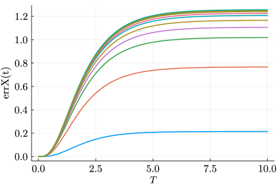
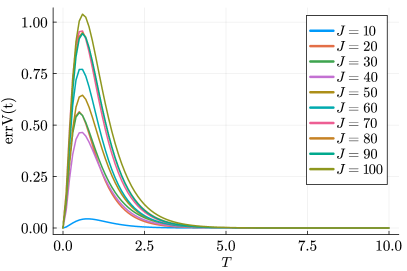
Figure 2: Evolution of $\mathbf{E}\texttt{errX(t)}$ and $\mathbf{E}\texttt{errV(t)}$, as defined in (6.2a) and (6.2b), for various values of $J$. We observe that $\mathbf{E}\texttt{errX(t)}$ initially increases, but tends to a constant in the limit $t\to\infty$ as flocking occurs.

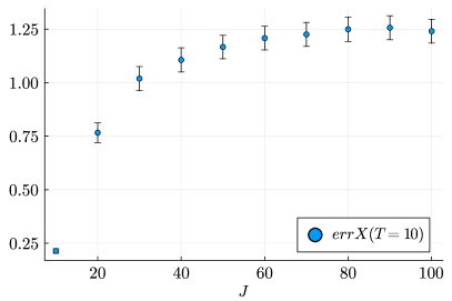
Figure 3: Value of $\mathbf{E}\texttt{errX(T)}$ for $T=10$ and various values of the system size $J$.

Acknowledgements

The authors are grateful to Franca Hoffmann, Dohyeon Kim and Julien Reygner for useful discussions and suggestions. UV is partially supported by the European Research Council (ERC) under the European Union’s Horizon 2020 research and innovation programme (grant agreement No 810367), and by the Agence Nationale de la Recherche under grants ANR-21-CE40-0006 (SINEQ) and ANR-23-CE40-0027 (IPSO).

References

• [1] Dirk Blömker, Claudia Schillings, Philipp Wacker and Simon Weissmann “Continuous time limit of the stochastic ensemble Kalman inversion: strong convergence analysis” In SIAM J. Numer. Anal. 60.6, 2022, pp. 3181–3215 DOI: 10.1137/21M1437561
• [2] Dirk Blömker, Claudia Schillings, Philipp Wacker and Simon Weissmann “Well posedness and convergence analysis of the ensemble Kalman inversion” In Inverse Problems 35.8, 2019, pp. 085007\bibrangessep32 DOI: 10.1088/1361-6420/ab149c
• [3] François Bolley, José A. Cañizo and José A. Carrillo “Stochastic mean-field limit: non-Lipschitz forces and swarming” In Math. Models Methods Appl. Sci. 21.11, 2011, pp. 2179–2210 DOI: 10.1142/S0218202511005702
• [4] François Bolley, Arnaud Guillin and Florent Malrieu “Trend to equilibrium and particle approximation for a weakly selfconsistent Vlasov-Fokker-Planck equation” In M2AN Math. Model. Numer. Anal. 44.5, 2010, pp. 867–884 DOI: 10.1051/m2an/2010045
• [5] J.. Carrillo, Y.-P. Choi, C. Totzeck and O. Tse “An analytical framework for consensus-based global optimization method” In Math. Models Methods Appl. Sci. 28.6, 2018, pp. 1037–1066 DOI: 10.1142/S0218202518500276
• [6] J.. Carrillo, M. Fornasier, J. Rosado and G. Toscani “Asymptotic flocking dynamics for the kinetic Cucker-Smale model” In SIAM J. Math. Anal. 42.1, 2010, pp. 218–236 DOI: 10.1137/090757290
• [7] Louis-Pierre Chaintron and Antoine Diez “Propagation of chaos: a review of models, methods and applications. I. Models and methods” In Kinet. Relat. Models 15.6, 2022, pp. 895–1015 DOI: 10.3934/krm.2022017
• [8] Louis-Pierre Chaintron and Antoine Diez “Propagation of chaos: a review of models, methods and applications. II. Applications” In Kinet. Relat. Models 15.6, 2022, pp. 1017–1173 DOI: 10.3934/krm.2022018
• [9] Young-Pil Choi, Seung-Yeal Ha and Zhuchun Li “Emergent dynamics of the Cucker-Smale flocking model and its variants” In Active particles. Vol. 1. Advances in theory, models, and applications, Model. Simul. Sci. Eng. Technol. Birkhäuser/Springer, Cham, 2017, pp. 299–331
• [10] Dan Crisan et al. “Poisson Equations with locally-Lipschitz coefficients and Uniform in Time Averaging for Stochastic Differential Equations via Strong Exponential Stability” In arXiv preprint 2204.02679, 2024
• [11] Felipe Cucker and Steve Smale “Emergent behavior in flocks” In IEEE Transactions on automatic control 52.5 IEEE, 2007, pp. 852–862
• [12] Zhiyan Ding and Qin Li “Ensemble Kalman inversion: mean-field limit and convergence analysis” In Stat. Comput. 31.1, 2021, pp. Paper No. 9\bibrangessep21 DOI: 10.1007/s11222-020-09976-0
• [13] Zhiyan Ding and Qin Li “Ensemble Kalman sampler: mean-field limit and convergence analysis” In SIAM J. Math. Anal. 53.2, 2021, pp. 1546–1578 DOI: 10.1137/20M1339507
• [14] Alain Durmus, Andreas Eberle, Arnaud Guillin and Raphael Zimmer “An elementary approach to uniform in time propagation of chaos” In Proc. Amer. Math. Soc. 148.12, 2020, pp. 5387–5398 DOI: 10.1090/proc/14612
• [15] Klaus-Jochen Engel and Rainer Nagel “A short course on operator semigroups”, Universitext Springer, New York, 2006
• [16] Massimo Fornasier, Timo Klock and Konstantin Riedl “Consensus-based optimization methods converge globally” In SIAM J. Opt. 34.3 SIAM, 2024, pp. 2973–3004
• [17] Nicolas Fournier and Arnaud Guillin “On the rate of convergence in Wasserstein distance of the empirical measure” In Probab. Theory Related Fields 162.3-4, 2015, pp. 707–738 DOI: 10.1007/s00440-014-0583-7
• [18] Nicolai Jurek Gerber, Franca Hoffmann and Urbain Vaes “Mean-field limits for Consensus-Based Optimization and Sampling” In arXiv preprint 2312.07373, 2023
• [19] Carl Graham and Denis Talay “Stochastic simulation and Monte Carlo methods” Mathematical foundations of stochastic simulation 68, Stochastic Modelling and Applied Probability Springer, Heidelberg, 2013 DOI: 10.1007/978-3-642-39363-1
• [20] Arnaud Guillin, Pierre Le Bris and Pierre Monmarché “Convergence rates for the Vlasov-Fokker-Planck equation and uniform in time propagation of chaos in non convex cases” In Electron. J. Probab. 27, 2022, pp. Paper No. 124\bibrangessep44 DOI: 10.1214/22-ejp853
• [21] Arnaud Guillin and Pierre Monmarché “Uniform long-time and propagation of chaos estimates for mean field kinetic particles in non-convex landscapes” In J. Stat. Phys. 185.2, 2021, pp. Paper No. 15\bibrangessep20 DOI: 10.1007/s10955-021-02839-6
• [22] Seung-Yeal Ha, Jeongho Kim and Xiongtao Zhang “Uniform stability of the Cucker-Smale model and its application to the mean-field limit” In Kinet. Relat. Models 11.5, 2018, pp. 1157–1181 DOI: 10.3934/krm.2018045
• [23] Seung-Yeal Ha and Jian-Guo Liu “A simple proof of the Cucker-Smale flocking dynamics and mean-field limit” In Commun. Math. Sci. 7.2, 2009, pp. 297–325 URL: http://projecteuclid.org/euclid.cms/1243443982
• [24] Seung-Yeal Ha and Eitan Tadmor “From particle to kinetic and hydrodynamic descriptions of flocking” In Kinet. Relat. Models 1.3, 2008, pp. 415–435 DOI: 10.3934/krm.2008.1.415
• [25] Hui Huang and Jinniao Qiu “On the mean-field limit for the consensus-based optimization” In Math. Methods Appl. Sci. 45.12, 2022, pp. 7814–7831
• [26] Marco A. Iglesias, Kody J.. Law and Andrew M. Stuart “Ensemble Kalman methods for inverse problems” In Inverse Problems 29.4, 2013, pp. 045001\bibrangessep20 DOI: 10.1088/0266-5611/29/4/045001
• [27] Marvin Koß, Simon Weissmann and Jakob Zech “On the mean field limit of consensus based methods” In arXiv preprint 2409.03518, 2024
• [28] Daniel Lacker “Hierarchies, entropy, and quantitative propagation of chaos for mean field diffusions” In Probab. Math. Phys. 4.2, 2023, pp. 377–432 DOI: 10.2140/pmp.2023.4.377
• [29] Daniel Lacker and Luc Le Flem “Sharp uniform-in-time propagation of chaos” In Probab. Theory Related Fields 187.1-2, 2023, pp. 443–480 DOI: 10.1007/s00440-023-01192-x
• [30] P.. Lax and R.. Richtmyer “Survey of the stability of linear finite difference equations” In Comm. Pure Appl. Math. 9, 1956, pp. 267–293 DOI: 10.1002/cpa.3160090206
• [31] F. Malrieu “Logarithmic Sobolev inequalities for some nonlinear PDE’s” In Stochastic Process. Appl. 95.1, 2001, pp. 109–132 DOI: 10.1016/S0304-4149(01)00095-3
• [32] Pierre Monmarché “Long-time behaviour and propagation of chaos for mean field kinetic particles” In Stochastic Process. Appl. 127.6, 2017, pp. 1721–1737 DOI: 10.1016/j.spa.2016.10.003
• [33] Sebastien Motsch and Eitan Tadmor “A new model for self-organized dynamics and its flocking behavior” In J. Stat. Phys. 144 Springer, 2011, pp. 923–947
• [34] Roberto Natalini and Thierry Paul “On the mean field limit for Cucker-Smale models” In Discrete Contin. Dyn. Syst. Ser. B 27.5, 2022, pp. 2873–2889 DOI: 10.3934/dcdsb.2021164
• [35] Benedetto Piccoli, Francesco Rossi and Emmanuel Trélat “Control to flocking of the kinetic Cucker-Smale model” In SIAM J. Math. Anal. 47.6, 2015, pp. 4685–4719 DOI: 10.1137/140996501
• [36] René Pinnau, Claudia Totzeck, Oliver Tse and Stephan Martin “A consensus-based model for global optimization and its mean-field limit” In Math. Models Methods Appl. Sci. 27.1, 2017, pp. 183–204 DOI: 10.1142/S0218202517400061
• [37] Katharina Schuh and Iain Souttar “Conditions for uniform in time convergence: applications to averaging, numerical discretisations and mean-field systems”, 2024
• [38] U. Vaes “Sharp propagation of chaos for the ensemble Langevin sampler” In J. London Math. Soc. 110.5, 2024, pp. e13008
• [39] Cédric Villani “Topics in Optimal Transportation” 58, Graduate Studies in Mathematics American Mathematical Society, Providence, RI, 2003 DOI: 10.1090/gsm/058