Improving accuracy of tree-tensor network approach by optimization of network structure

Abstract

Numerical methods based on tensor networks have been extensively explored in the research of quantum many-body systems in recent years. It has been recognized that the ability of tensor networks to describe a quantum many-body state crucially depends on the spatial structure of the network. In the previous work, we proposed an algorithm based on tree tensor networks (TTNs) that automatically optimizes the structure of TTN according to the spatial profile of entanglement in the state of interest. In this paper, we precisely analyze how detailed updating schemes in the structural optimization algorithm affect its computational accuracy for the random XY-exchange model under random magnetic fields and the Richardson model. We then find that for the random XY model, on the one hand, the algorithm achieves improved accuracy, and the stochastic algorithm, which selects the local network structure probabilistically, is notably effective. For the Richardson model, on the other hand, the resulting numerical accuracy subtly depends on the initial TTN and the updating schemes. In particular, the algorithm without the stochastic updating scheme certainly improves the accuracy, while the one with the stochastic updates results in poor accuracy due to the effect of randomizing the network structure at the early stage of the calculation. These results indicate that the algorithm successfully improves the accuracy of the numerical calculations for quantum many-body states, while it is essential to appropriately choose the updating scheme as well as the initial TTN structure, depending on the systems treated.

I Introduction

Since the development of the density-matrix renormalization-group (DMRG) method[1, 2], tensor-network approach has made rapid progress in a variety of fields[3, 4, 5]. While tensor networks have been studied in statistical mechanics for long years[6], the introduction of quantum-information concepts has advanced the understanding of their properties significantly, and it has been recognized that tensor networks can represent the low-energy states of quantum many-body systems efficiently. Several algorithms based on various tensor-network states, including matrix-product state (MPS)[7, 8], tensor-product state (TPS)[9, 10] or projected entangled-pair state (PEPS)[11, 12], and the state of multiscale entanglement renormalization ansatz (MERA)[13, 14], have been developed.

A tensor network is a contraction of low-rank tensors and is utilized as an approximation of a high-rank tensor such as a wave function of a quantum many-body state. In general, the number of elements of the high-rank tensor increases exponentially with the number of quantum spins (qudits) in the system. One can avoid this exponential growth of the Hilbert space by setting an upper bound on the dimension of the auxiliary bonds in the tensor network. The drawback of introducing the upper bound on the bond dimension is the loss of accuracy due to the truncation of the Hilbert space. How to reduce this loss is an essential issue in tensor-network approaches.

In this paper, we explore a numerical algorithm based on the tree-tensor networks (TTNs), which are tensor networks without loops. We particularly focus on binary trees, TTNs composed of three-leg tensors, although the extension to $m$-ary trees is straightforward. An essential property of the TTN is that it can be separated into two parts by cutting an arbitrary bond in the network. This property of TTN leads to the following guideline for reducing the loss of accuracy by truncation.[15, 16, 17] Since every bond in a TTN has a corresponding bipartition of the system, each bond must be able to represent the quantum entanglement between the subsystems of the corresponding bipartition. However, due to the upper bound of the bond dimension, which we denote by $\chi$ in the following, the entanglement entropy (EE) that a bond can carry is also upper bounded to a maximum of $\ln\chi$. If the EE associated with each bond exceeds the upper limit, the excess entanglement is omitted in the approximated TTN and results in a loss of accuracy. Here, recall that the number of bonds in a TTN, which is $2N-3$ where $N$ is the number of quantum spins in the system, is much smaller than the number of the possible bipartitions of the system, $2^{N-1}-1$. Therefore, the network structure that makes the EEs on the $(2N-3)$ bonds as small as possible can minimize the loss of accuracy in approximating the target quantum state by a TTN with a finite $\chi$. We call this guideline to minimize the EEs on a TTN the least-EE principle.

The least-EE principle indicates that using a TTN with the optimal structure is crucially important for improving the accuracy of the TTN approach. However, finding the optimal TTN structure is highly nontrivial and challenging. Several efforts have been devoted to the problem so far. There have been attempts to optimize the order of sites within the matrix-product network (MPN), which is employed in DMRG, based on various guidelines.[18, 19, 20, 21, 22] A method to optimize the structure of TTN using the cut-off bond dimension as a minimization function has also been proposed.[23] For systems with randomness, the tensor-network strong-disorder renormalization group (tSDRG) method, in which a TTN suitable for a random system of interest is constructed based on the idea of the strong-disorder renormalization group,[24, 25] has been developed[26, 27] and successfully applied.[28, 29, 15] For small systems for which exact wavefunction is obtained, a method to extract the optimal TTN structure from the wavefunction according to the least-EE principle has also been proposed.[17]

In the previous study[16], we proposed an algorithm to search for the optimal TTN structure by iterating the local reconstruction of the network based on the least-EE principle. We applied the algorithm to some toy models for which the optimal TTN structure was deduced from the perturbative renormalization analysis[16, 30]. We then demonstrated that the algorithm succeeded in obtaining the expected optimal structure. In this paper, we investigated the performance of several types of the TTN structural optimization calculations, which are specified by the initial TTN structure, the scheme to select the local TTN structure in the optimization process, and the bond dimension at which the structural optimization is executed. We performed the calculations of the types on the random XY-exchange model under random magnetic fields and the Richardson model. We thereby demonstrated that for the random XY model, the structural optimization algorithm could reduce the variational energy significantly. In particular, stochastic schemes, which select the local TTN structure probabilistically, achieved the lowest variational energy regardless of the initial TTN structure. For the Richardson model, we found that while the structural optimization algorithm could yield a good TTN structure with a low variational energy, the calculations were sometimes trapped by a TTN structure unsuitable for representing the lowest energy state and failed to reach the optimal TTN structure. These results for the two models reveal that while the TTN structural optimization algorithm is basically effective in improving the accuracy of the calculation, the performance of each type of the calculations depends on the model. The results thus indicate the importance of appropriately choosing the updating scheme of the network and the initial TTN structure according to the model to be studied.

The plan of this paper is as follows. In Sec. II, we review the structural optimization algorithm and make several comments. Section III.1 describes the types of the optimization calculation tested in the present study and the quantities calculated. Sections III.2 and III.3 respectively present the numerical results for the random XY-exchange model under random magnetic fields and the Richardson model. The performances of each type for the models are discussed there. Section IV is devoted to a summary and concluding remarks. In Appendix A, we explain how to prepare the initial TTN. The details of the actual calculation, including the number of sweeps, are presented in Appendix B. Appendix C describes the exact calculation of the lowest energy for the Richardson model.

II Algorithm

The algorithm we study in this work is the one proposed in Ref. [16]. Here, we briefly review the algorithm for completeness and add comments. We note that an algorithm to optimize the site ordering within the MPN based on a similar strategy has been proposed in Ref. [22].

In the proposed algorithm, the wave function of the quantum state is represented by a TTN. Figure 1 shows typical examples of TTNs. We note that the TTN includes MPN, which is employed in the DMRG method, and the perfect-binary tree (PBT).

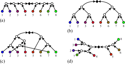
Figure 1: Examples of TTN. (a) Matrix-Product Network (MPN), (b) Perfect-Binary Tree (PBT), (c) TTN of a generic form, and (d) the same TTN as that in (c). Open circles represent isometries and the solid diamond represents the singular-value matrix. Circles with colors represent bare spins. In (a), (b), and (c), the bare spins are arranged in the order of the site index. Note that within the category of MPN and PBT, there are many networks with different site orderings.

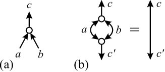
Figure 2: (a) Isometry $V_{a,b}^{c}$ with the legs $a$, $b$, and $c$. (b) Schematic picture of the orthonormal condition Eq. (1). Connected legs (bonds) represent a contraction of their degrees of freedom. The connected arrows in the right-hand-side of (b) represents a Kronecker delta $\delta_{cc^{\prime}}$.

Let us write a tensor in the TTN as $V_{a,b}^{c}$ as in Fig. 2 (a). We impose the orthonormal condition on $V_{a,b}^{c}$,

$$\sum_{a,b}\bar{V}_{a,b}^{c}V_{a,b}^{c^{\prime}}=\delta_{cc^{\prime}},$$ (1)

where $\bar{V}_{a,b}^{c}$ is a complex conjugate of $V_{a,b}^{c}$, and call the tensor the isometry. We assign a direction to each bond in the TTN so that the bases of the bond outgoing from each tensor are orthonormal; Namely, in Eq. (1), the index $c$ ($c^{\prime}$) corresponds to the outgoing bond, while the indices $a$ and $b$ correspond to the incoming bonds. All bonds in the TTN are directed from the boundary, where the bare spin degrees of freedom are, towards the “center” of the TTN, where the diagonal matrix of singular values is located. Such a representation format of the TTN is called the mixed canonical form[31]. Adopting the mixed canonical form offers strong advantages, such as guaranteeing the orthonormality of the basis of the truncated Hilbert space expanded by incoming bonds and making the contraction caluculations of isometries extremely simple as shown in Fig. 2 (b). We note that the center position of the canonical form can be taken at an arbitrary bond and can also be moved by the fusing and re-decomposing process of tensors[31].

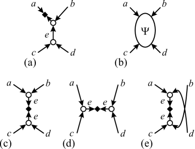
Figure 3: (a) Central area at the biginning of a step. (b) Effective ground-state wave function $\Psi(abcd)$ obtained by the diagonalization of the effective Hamiltonian $\tilde{\mathcal{H}}$. (c), (d), and (e) show the possible local connections of the singular-value decomposition Eqs. (2a), (2b), and (2c), respectively. Open circles represent isometries and a solid diamond denotes the singular-value matrix at the canonical center.

Table 1: Algorithm to optimize the structure and isometries of TTN.

1.	Prepare an initial TTN expressed in the mixed canonical form. (See Appendix A for the detail.)
2.	Construct the effective Hamiltonian $\tilde{\mathcal{H}}$ of the whole system on the orthogonal basis of the central area.
3.	Diagonalize the effective Hamiltonian $\tilde{\mathcal{H}}$ to obtain the ground-state wave function $\Psi$.
4.	Perform the singular-value decomposition of $\Psi$ for the three possible local connections in Figs. 3 (c)-(e).
5.	Choose the optimal local connection according to the adopted updating scheme of the network discribed
	in the text of Sec. II and Sec. III.1.
6.	Update the local structure of TTN as well as isometries in the central area.
7.	Move the central area according to the sweeping rule. (See Ref. [16] for the details of the rule.)
8.	Iterate processes 2. - 7. until the sweep of the entire TTN is completed.

The algorithm optimizes the structure and isometries of TTN in the following manner. In the TTN, we focus on the “central area”, depicted in Fig. 3 (a), which consists of the diagonal matrix of singular values at the canonical center located on the bond $a$ and two isometries connected to it. The Hilbert space for the central area is expanded by the orthonormal basis of the incoming bonds $a,b,c$, and $d$, and we can construct the effective Hamiltonian $\tilde{\mathcal{H}}$ of the whole system represented in the (truncated) Hilbert space. Then, we diagonalize the effective Hamiltonian using, e.g., the Lanczos method to obtain the ground-state wave function $\Psi(abcd)$ [Fig. 3 (b)]. Next, we perform the singular-value decomposition of $\Psi(abcd)$ for the three possible local connections of the isometries [see Figs. 3 (c)-(e)],

$$\Psi(abcd)=\sum_{e=1}^{\chi^{2}}V^{e}_{ab}D_{e}V^{e}_{cd},$$ (2a)

$$\Psi(abcd)=\sum_{e=1}^{\chi^{2}}V^{e}_{ac}D^{\prime}_{e}V^{e}_{bd},$$ (2b)

$$\Psi(abcd)=\sum_{e=1}^{\chi^{2}}V^{e}_{ad}D^{\prime\prime}_{e}V^{e}_{bc}.$$ (2c)

Throughout this paper, we distinguish the isometries by the letters for the bond index, if necessary. [Hence, for example, $V^{e}_{ab}$ and $V^{e}_{cd}$ in Eq. (2a) are different isometries.] We also adopt the notation that the singular values are arranged in the descending order, $D_{1}\geq D_{2}\geq\cdots\geq D_{\chi^{2}}\geq 0$ (the same for $\{D^{\prime}_{e}\}$ and $\{D^{\prime\prime}_{e}\}$) and suppose that the ground-state wave function $\Psi(abcd)$ is normalized so that $\sum_{e=1}^{\chi^{2}}(D_{e})^{2}=\sum_{e=1}^{\chi^{2}}(D^{\prime}_{e})^{2}=\sum_{e=1}^{\chi^{2}}(D^{\prime\prime}_{e})^{2}=1$. Since the spectra of the singular values, $\{D_{e}\}$, $\{D^{\prime}_{e}\}$, and $\{D^{\prime\prime}_{e}\}$, are different from each other, the EEs obtained from those singular values,

$$\mathcal{S}^{(ab|cd)}=-\sum_{e=1}^{\chi^{2}}(D_{e})^{2}\ln(D_{e})^{2},$$ (3a)

$$\mathcal{S}^{(ac|bd)}=-\sum_{e=1}^{\chi^{2}}(D^{\prime}_{e})^{2}\ln(D^{\prime}_{e})^{2},$$ (3b)

$$\mathcal{S}^{(ad|bc)}=-\sum_{e=1}^{\chi^{2}}(D^{\prime\prime}_{e})^{2}\ln(D^{\prime\prime}_{e})^{2},$$ (3c)

are also different. Therefore, we can select the connection of the isometries with the smallest EE as the optimal one to update the local structure of TTN. Simultaneously, we can update the isometries in the central area by replacing them with the tensors obtained from the adopted singular-value decomposition, where we truncate the dimension of the center bond $e$ by keeping only the bases with the $\chi$-largest singular values.[32] We call the above procedures to update the local network structure and the isometries of the TTN [from Fig. 3(a) to Fig. 3(c)-(e)] a step. When this step is completed, we shift the central area by one isometry according to an appropriate sweeping rule of the network[16] and continue the computation. We iterate the steps by sweeping the entire network to obtain the optimal TTN. The algorithm is summarized in Table. 1.

Several comments on the algorithm are presented in order below.

In the structural optimization, the above-mentioned algorithm adopts the least-EE principle to choose the local network connection that minimizes the EE on the center bond. There are other options here. First, one may select the local connection that minimizes the truncated reduced density-matrix (rDM) weight[22], the sum of the rDM eigenvalues for the discarded bases, defined as

$$\delta\rho_{\rm cut}^{(ab|cd)}=\sum_{e=\chi+1}^{\chi^{2}}(D_{e})^{2},$$ (4a)

$$\delta\rho_{\rm cut}^{(ac|bd)}=\sum_{e=\chi+1}^{\chi^{2}}(D^{\prime}_{e})^{2},$$ (4b)

$$\delta\rho_{\rm cut}^{(ad|bc)}=\sum_{e=\chi+1}^{\chi^{2}}(D^{\prime\prime}_{e})^{2}.$$ (4c)

While both criteria using the EE of the center bond [Eq. (3)] or the truncated rDM weight [Eq. (4)] should work in searching for a good TTN structure, it is expected that using the latter is advantageous to improve the computational accuracy as much as possible with a fixed $\chi$ since the truncated rDM weight is directly related to the fidelity of the variational wave function in TTN with that of the true ground state. On the other hand, using the bond EE directly observes the entanglement and, therefore, is expected to be suitable to grasp the entanglement geometry of the ground state. It also bears noting that the algorithm using the truncated rDM weight should be strongly dependent on $\chi$.

Second, since the reconnection of the network performed in the algorithm is local, the structural optimization may be trapped by local minima in the landscape of network structure, especially when the system contains complexity such as randomness. A possible strategy to avoid such traps is to implement a stochastic selection of the network structure. Namely, one may select the local connection randomly from the three possible candidates according to the probabilities,

$$P^{(1)}\propto\exp(-\beta\mathcal{S}),$$ (5)

where $\mathcal{S}=\mathcal{S}^{(ab|cd)},\mathcal{S}^{(ac|bd)},\mathcal{S}^{(ad|bc)}$ is the EE at the center bond of each local connection. $\beta$ is an effective inverse temperature that is increased as the calculation proceeds. Also, if one prefers the heavier penalty for the connection with the larger bond EE, one may use the probabilities,

$$P^{(2)}\propto\exp(-\beta\mathcal{S}^{2}).$$ (6)

In the algorithm described above, one can improve only the isometries in the TTN with leaving the TTN structure fixed by always choosing the local connection $(ab|cd)$ for the singular-value decomposition Eq. (2a) at the process 5 in Table 1. Therefore, in practice, we can easily switch the calculations with and without the structural optimization of TTN. In our calculation discussed in the subsequent sections, we first perform the calculation with structural optimization at a certain $\chi=\chi_{\rm opt}$. Then, we continue the calculation without structural optimization with increasing $\chi$ to further improve the isometries in the TTN having the optimized structure.

In the singular-value decomposition of the wave function $\Psi(abcd)$, the number of non-zero singular values (the rank of the wave-function matrix in the decomposition considered) may be smaller than $\chi$. In such a case, only the bases corresponding to the non-zero singular values are adopted as the new bases for the center bond. In the practical calculation, bases with singular values smaller than a certain threshold (set to be $10^{-6}$ in our calculation) are discarded since their contribution to the wave function is negligibly small. In this case, which often occurs for the bonds close to the boundary of the TTN, the dimension of the bond is smaller than the upper bound $\chi$. Furthermore, in our calculation, all the bases whose singular values are degenerate are kept or discarded altogether to preserve symmetries of the target state. This measure may also result in an auxiliary bond with a dimension smaller than $\chi$.

In the calculation of the algorithm, one must be careful about the case that the dimensions of all three legs of an isometry become unity, which traps the calculation. Suppose that the dimensions of the bonds $a$, $b$, and $e$ are all unity in the situation shown in Fig. 3 (a). Then, the singular value of the connection with no structural change, shown in Fig. 3 (c), are $D_{1}=1$, $D_{e}=0$ $(e\geq 2)$, and the EE and truncated rDM weight are zero, which should be minimum among the three possible connections. As a result, the connection of Fig. 3 (c) will be selected, and the dimensions of the bonds $a$, $b$, and $e$ remain unity. (If the stochastic selection is adopted, there is a possibility that the other structure will be selected, but the original structure is most likely to be selected even in this case.) In such a way, the calculation can be stuck in the TTN containing the isometry whose three legs represent only one basis. In our calculation discussed in Sec. III, the problem occurred in some cases of the calculations of the Richardson model. We avoided the problem by taking an exceptional treatment in the preparation of the initial TTN. See Sec. III.3 and Appendix A for the details.

III Numerical results

III.1 Types of calculation and Quantities computed

We have applied the algorithm discussed in the previous section to the random XY-exchange model under random magnetic field and the Richardson model. In the calculation, we can choose (i) the initial TTN, (ii) the scheme to update the local TTN structure, and (iii) the value of $\chi$ with which the structural optimization is performed. We have carried out various types of calculations specified by (i), (ii), and (iii) and compared them to evaluate their performance. The types of calculations performed are in the following.

• Initial TTN

  • MPN: We prepared the MPN as the initial TTN. The bare spins were arranged one-dimensionally in the order of the site index and the canonical center is located at the center of the MPN, as shown in Fig. 1 (a).

  • PBT: We prepared the PBT as the initial TTN. The bare spins were arranged one-dimensionally in the order of the site index and the canonical center is located at the “top” of the PBT, as shown in Fig. 1 (b).

  • TTN constructed by tSDRG method: We prepared the initial TTN using the tSDRG, which is a method to construct a TTN suitable to represent the ground state of a system with randomness. See Ref. [29] for the details. We adopted the gap $\Delta^{\rm I}_{\rm max}$ defined in Ref. [29] to determine the order of the isometries to be merged. This initial TTN constructed by tSDRG was used only for the random XY model.

  The isometries in the initial TTN were composed of the $\chi$-lowest-energy eigenvectors of the block Hamiltonian of the subsystem consisting of the spins that belong to the incoming bonds of each isometry, as in Ref. [16]. For the Richardson model, an exceptional treatment was adopted to avoid the problem of the isometry with three legs having the dimension unity, as discussed in the previous section. See Appendix A for details.

• Scheme to update local TTN structure

  • No structural optimization: The TTN structure was fixed to the one of the initial TTN, and only the isometries were improved. This calculation is equivalent to the conventional variational TTN calculation.

  • Adopt the local structure with the smallest EE: We optimized the TTN structure by adopting the local connection that gave the smallest EE among the EEs defined in Eq. (3).

  • Adopt the local structure with the smallest truncated rDM weight[22]: We optimized the TTN structure by adopting the local connection that gave the smallest truncated rDM weight among the ones defined in Eq. (4). If there were multiple local connections with the weight $\delta\rho$ smaller than $10^{-11}$, we judged that their difference was negligible and adopted the local connection that gave the smallest EE among them.

  • Stochastic selection using the probability $P^{(1)}$: We optimized the TTN structure by selecting the local connection stochastically according to the probability defined by Eq. (5). For the effective inverse temperature, we employed the exponential form,

    $$\beta=\beta_{0}~2^{n/n_{\tau}}$$ (7)

    where $n$ was the sweep number and $(\beta_{0},n_{\tau})$ were control parameters.

  • Stochastic selection using the probability $P^{(2)}$: We optimized the TTN structure by selecting the local connection stochastically according to the probability defined by Eq. (6). The effective inverse temperature was treated in the same way as in (D).

• $\chi$ for the structural optimization
  In schemes (B)-(E) in (ii), we first performed the structural optimization calculation with $\chi=\chi_{\rm opt}$ to determine the optimal TTN structure. After that, the isometries were further improved with increasing $\chi$ in the TTN with the structure fixed to the optimized one. In the actual calculation for the random XY model (the Richardson model), we performed the structural optimization at $\chi_{\rm opt}=16$ or $32$ ($20$ or $40$), and then continued the calculation to optimize isometries with increasing $\chi$ up to $40$ ($80$). The details, including the number of sweeps and the criteria for judging convergence are given in Appendix B.

At each step of the calculation, we computed the lowest energy eigenvalue $E_{0}$ of the effective Hamiltonian $\tilde{\mathcal{H}}$ constructed for the central area and the EE on the center bond. We then adopted the lowest $E_{0}$ obtained in a sweep as the variational energy at the sweep. Here, it should be noted that $E_{0}$ is the eigenvalue of the effective Hamiltonian expressed in the Hilbert space expanded by the four bonds $a,b,c$, and $d$ in Fig. 3(b), and the corresponding eigenstate $\Psi(abcd)$, that is expressed as Eq. (2) is not strictly the same as the TTN state in the sense that the center bond does not suffer from the cutoff. Therefore, as a wave function corresponding to the TTN state in which the dimensions of all bonds are upper bounded by $\chi$, we constructed the truncated wave function as

$$|\tilde{\Psi}\rangle=\sum_{abcd}\tilde{\Psi}(abcd)|abcd\rangle,$$ (8a)

$$\tilde{\Psi}(abcd)=\sum_{e=1}^{\chi}V_{ab}^{e}D_{e}V_{cd}^{e},$$ (8b)

for the case that the local connection $(ab|cd)$ [Fig. 3 (c)] was selected, and by similar ways for the other connections. We then calculate the expectation value of the effective Hamiltonian on the truncated state as

$$E^{\prime}_{0}=\frac{\langle\tilde{\Psi}|\tilde{\mathcal{H}}|\tilde{\Psi}\rangle}{\langle\tilde{\Psi}|\tilde{\Psi}\rangle}.$$ (9)

[Note that the truncated wave function $|\tilde{\Psi}\rangle$ defined in Eq. (8) is not strictly normalized.] We will analyze $E^{\prime}_{0}$ in the same way as $E_{0}$.

III.2 Random XY-exchange Model Under Random Magnetic Field

We have applied the TTN structural optimization algorithm to the spin-1/2 model with random XY-exchange interactions under random magnetic field. The model Hamiltonian is given by

$$\mathcal{H}_{\rm r}=\frac{J_{\rm r}}{\sqrt{N}}\sum_{i=1}^{N-1}\sum_{j=i+1}^{N}\epsilon_{ij}\left(S^{x}_{i}S^{x}_{j}+S^{y}_{i}S^{y}_{j}\right)-\sum_{i=1}^{N}h_{i}S^{z}_{i},$$

(10)

where $J_{\rm r}$ is a parameter to control the strength of the exchange interactions and ${\bm{S}}_{i}=(S^{x}_{i},S^{y}_{i},S^{z}_{i})$ is the spin-1/2 operator at $i$ th site. $\epsilon_{ij}$ and $h_{i}$ are random variables obeying uniform distributions in the range $[0,1]$ and $\left[-\frac{1}{2},\frac{1}{2}\right]$, respectively. We have performed the calculations for the case of the exchange constant $J_{\rm r}=8$ and the system size $N=64$. In the calculations, we have prepared $\mathcal{N}_{\rm s}=200$ random samples and computed the lowest-energy state in the subspace with zero total magnetization, $\sum_{i}S^{z}_{i}=0$. Note that this state may not be the ground state of each random sample, depending on the random model parameters $\{\epsilon_{ij}\}$ and $\{h_{i}\}$.

We have employed MPN, PBT, and the TTN obtained by tSDRG [(1), (2), and (3) introduced in Sec. III.1] as the initial TTN structure and performed the calculations of schemes (A)-(E). In scheme (A) (without TTN structural optimization), we optimized isometries in the TTN with fixed structure with sequentially increasing $\chi$ from $16$ to $40$. For schemes (B)-(E), two cases of calculations were performed: in one case, the TTN structural-optimization calculation was executed with $\chi=\chi_{\rm opt}=16$, and in the other case, the calculation was done with $\chi=\chi_{\rm opt}=32$. After that, we fixed the TTN structure and optimized only isometries with increasing $\chi$ up to $40$. See Appendix B for details. Thus, the type of calculation is specified by three conditions: initial TTN [(1)-(3)], optimization scheme [(A)-(E)], and $\chi_{\rm opt}$ ($=16$ or $32$) with which the TTN structural optimization was performed. For the stochastic structural optimization [schemes (D) and (E)], we performed two runs of the calculation with the different annealing parameters, $(\beta_{0},n_{\tau})=(0.1,2),(0.1,4)$, in Eq. (7). Then, among the results of the two runs, we adopted the one obtained by the run that gives the smaller variational energy $E_{0}$ ($E^{\prime}_{0}$) at $\chi=40$ as the lowest energy used in the analysis of random average of $\delta r$ ($\delta r^{\prime}$) defined below.

To evaluate the performance of each type of calculation, we explore the relative reduction in the variational energy with respect to the energy obtained by the calculation of the fixed structure of MPN [type (1A)] at $\chi=16$,

$$\delta r(\nu,{\rm X},\chi) = \frac{E_{0}(\nu,{\rm X},\chi)-E_{0}(\nu,{\rm 1A},16)}{|E_{0}(\nu,{\rm 1A},16)|},$$ (11)

$$\delta r^{\prime}(\nu,{\rm X},\chi) = \frac{E^{\prime}_{0}(\nu,{\rm X},\chi)-E^{\prime}_{0}(\nu,{\rm 1A},16)}{|E^{\prime}_{0}(\nu,{\rm 1A},16)|},$$ (12)

where $E^{(^{\prime})}_{0}(\nu,{\rm X},\chi)$ is the variational energy obtained by the calculation of type ${\rm X}$ at the bond dimension $\chi$ for the random sample $\nu=1,...,\mathcal{N}_{\rm s}$. We then examine the random average of $\delta r(\nu,{\rm X},\chi)$ and $\delta r^{\prime}(\nu,{\rm X},\chi)$, respectively denoted as $[\delta r({\rm X},\chi)]$ and $[\delta r^{\prime}({\rm X},\chi)]$. ($[\cdots]$ denotes the average over $\mathcal{N}_{\rm s}$ random samples.) In the following, we present only the results of $[\delta r({\rm X},\chi)]$ since we have found that $[\delta r({\rm X},\chi)]$ and $[\delta r^{\prime}({\rm X},\chi)]$ lead to essentially the same conclusions.

Figure 4 shows the random average $[\delta r({\rm X},\chi)]$ as a function of $\chi$. Also, the values of $[\delta r({\rm X},\chi=40)]$ for all types are plotted in Fig. 5. The magnitude of the error bar for the random average $[\delta r({\rm X},\chi)]$ shown in the figure is obtained as

$$\sigma_{r}=\sqrt{\frac{1}{\mathcal{N}_{\rm s}(\mathcal{N}_{\rm s}-1)}\sum_{\nu=1}^{\mathcal{N}_{\rm s}}\left\{\delta r(\nu,{\rm X},\chi)-[\delta r({\rm X},\chi)]\right\}^{2}}.$$

(13)

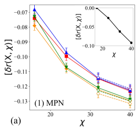
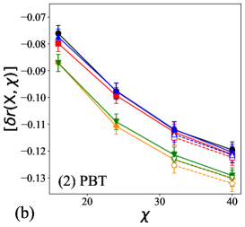
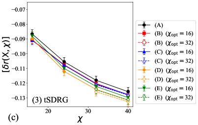
Figure 4: Random averages of the relative reduction in the variational energy, $[\delta r({\rm X},\chi)]$, as functions of $\chi$, for the types where the initial TTN is (a) (1) MPN, (b) (2) PBT, and (c) (3) TTN obtained by tSDRG. In (a), the data for type (1A) are shown in the inset.

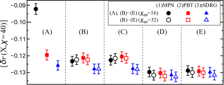
Figure 5: Random averages of the relative reduction in the variational energy, $[\delta r({\rm X},\chi)]$, at $\chi=40$. Circles, squares, and triangles represent the results of the types where the initial TTN is (1) MPN, (2) PBT, and (3) TTN obtained by tSDRG, respectively. Solid symbols represent the results of (A) or (B)-(E) with $\chi_{\rm opt}=16$, while open symbols are those of (B)-(E) with $\chi_{\rm opt}=32$.

In the calculation without structural optimization [scheme (A)], (1) MPN has the poorest accuracy in variational energies, whereas (2) PBT and (3) TTN obtained by tSDRG yield the results with relatively good accuracy. As for the results of non-stochastic structural optimization [schemes (B) and (C)], a significant improvement is observed when the initial TTN is MPN, reflecting the poor accuracy of the MPN calculation without structural optimization. When the initial TTN is PBT or that of tSDRG, there is an improvement in accuracy although it is small. Besides, when the initial TTN is MPN and PBT [(1B), (1C), (2B), and (2C)], the accuracy in the variational energies is worse than that of the tSDRG without structural optimization (3A). These results suggest that the structural optimization calculations with schemes (B) and (C) retain the influence of the initial TTN and are trapped in the vicinity of the initial TTN in the TTN-structure space. (Incidentally, this observation indicates the effectiveness of tSDRG for the random XY model.) We note that there is no notable difference between the results of schemes (B) and (C); namely, the performance of the schemes to minimize EE and that to minimize the truncated rDM weight is comparable, at least for the random XY model and $\chi_{\rm opt}$ treated. In the calculations of the stochastic structural optimizations [schemes (D) and (E)], the variational energy is further reduced, yielding the best accuracy for the calculations performed here. Of particular importance is the fact that the results of these schemes achieve almost the same level of accuracy independent of the initial TTN. These results suggest that the stochastic structural optimizations work well for the random XY model and succeed in escaping the influence of the initial TTN. Comparing the results of schemes (D) and (E), scheme (D) yields slightly lower variational energy, if any. However, the difference is small and remains within the error of the random sampling average.

Finally, concerning the effect of $\chi_{\rm opt}$ at which the structural optimization is performed, the results of $\chi_{\rm opt}=32$ yield slightly lower variational energy than those of $\chi_{\rm opt}=16$ in the stochastic structural optimization calculations [schemes (D) and (E)]. However, the difference is within the statistical error and basically smaller than the difference between stochastic optimizations [schemes (D) and (E)] and non-stochastic ones [schemes (B) and (C)]. This observation indicates that the value of $\chi_{\rm opt}$ has only a minor effect comparing the difference in the initial TTN and the updating scheme, at least within the range of $\chi$ we treated here.

Next, we discuss EE on each bond of TTN. Since EE on the physical bonds, the bonds directly connected to the bare spins, takes the same value regardless of the TTN structure, we consider only the EEs on the auxiliary bonds in the following analysis. In the analysis, we use the data of EEs obtained in the sweep which yields the lowest variational energy $E_{0}$ among the sweeps iterated at each $\chi$. For the stochastic schemes [schemes (D) and (E)], we use the EEs obtained by the run that yields the lower variational energy $E_{0}$ at $\chi=40$ between the two runs with different annealing parameters.

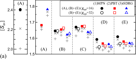
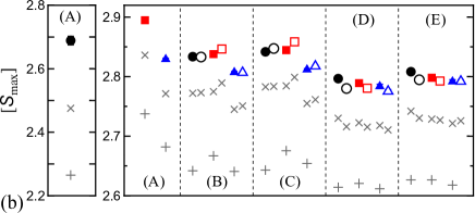
Figure 6: (a) $\left[\mathcal{S}_{\rm av}\right]$ and (b) $\left[\mathcal{S}_{\rm max}\right]$, that are respectively the random averages of the average values $\mathcal{S}_{\rm av}(\nu)$ and maximum values $\mathcal{S}_{\rm max}(\nu)$ of EEs on auxiliary bonds in each random sample. Circles, squares, and triangles represent the results at $\chi=40$ of the types where the initial TTN is (1) MPN, (2) PBT, and (3) TTN obtained by tSDRG, respectively. Solid symbols represent the results of (A) or (B)-(E) with $\chi_{\rm opt}=16$, while open symbols are those of (B)-(E) with $\chi_{\rm opt}=32$. Grey crosses represent the results at $\chi=32$ ($\times$) and $\chi=24$ ($+$); the latter presents only for (A) and (B)-(E) with $\chi_{\rm opt}=16$. The results for (1A) are plotted in a different scale for the clarity. Error bars are plotted only for the results at $\chi=40$, although they are smaller than the symbols in most cases.

To see how the EEs in the TTN are suppressed by the structural optimization, we explore the average and maximum values of EE. Figure 6 shows the random averages of $\mathcal{S}_{\rm av}(\nu)$ and $\mathcal{S}_{\rm max}(\nu)$, $\left[\mathcal{S}_{\rm av}\right]$ and $\left[\mathcal{S}_{\rm max}\right]$, where $\mathcal{S}_{\rm av}(\nu)$ and $\mathcal{S}_{\rm max}(\nu)$ are respectively the average and maximum values of EE on the auxiliary bonds in each random sample. Error bars are obtained by a formula similar to Eq. (13). We note that $\left[\mathcal{S}_{\rm av}\right]$ and $\left[\mathcal{S}_{\rm max}\right]$ are increasing functions of $\chi$, and one should analyze them at a sufficiently large $\chi$ to compare the TTNs obtained by different types of structural optimization.

For the average EE, $\left[\mathcal{S}_{\rm av}\right]$, the result for the MPN without structural optimization (1A) is remarkably large and has a pronounced $\chi$ dependence compared to other data, where the convergence with respect to $\chi$ is almost achieved at $\chi=40$. This observation indicates that in the MPN, there is a significant fraction of auxiliary bonds whose EEs are too large to be borne even by a bond with $\chi=40$. The values of $\left[\mathcal{S}_{\rm av}\right]$ of PBT and tSDRG without structural optimization [(2A) and (3A)] are much smaller than that of MPN (1A). The non-stochastic structural optimization [schemes (B) and (C)] reduces $\left[\mathcal{S}_{\rm av}\right]$ for MPN and tSDRG, while no notable reduction is observed for PBT. Furthermore, for all initial TTNs, the values of $\left[\mathcal{S}_{\rm av}\right]$ obtained by schemes (B) and (C) are larger than those of stochastic structural optimization [schemes (D) and (E)]. These observations suggest that the non-stochastic structural optimization by schemes (B) and (C), especially when applied to PBT, is trapped around the initial TTN in the TTN structural space. Finally, the results of $\left[\mathcal{S}_{\rm av}\right]$ obtained by the stochastic structural optimization [schemes (D) and (E)] achieve the smallest values independently of the initial TTNs, although there is some exception of the types (1D) and (1E) with $\chi_{\rm opt}=16$ which yield slightly large values. This result demonstrates the effectiveness of the stochastic optimization for the random XY model. As for the dependence of the results on $\chi_{\rm opt}$, the difference between $\left[\mathcal{S}_{\rm av}\right]$ obtained by each type with $\chi_{\rm opt}=16$ and $\chi_{\rm opt}=32$ is basically small compared to the difference due to the initial TTN or the updating scheme [except for (1D) and (1E)], indicating that the effect of $\chi_{\rm opt}$ is secondary.

The data of $\left[\mathcal{S}_{\rm max}\right]$ suffer from relatively large $\chi$ dependence, however, they lead us to the following conclusions that are basically consistent with the ones we read from the data of $[\mathcal{S}_{\rm av}]$: That is, the results of scheme (A) exhibit specific behaviors reflecting the characteristics of each TTN. [We note that $[\mathcal{S}_{\rm max}]$ for (1A) at $\chi=40$ is smaller than those for other types, but its large $\chi$ dependence implies that $[\mathcal{S}_{\rm max}]$ for (1A) may be greater than those for other types at $\chi\to\infty$.] The results of the non-stochastic schemes [schemes (B) and (C)] exhibit a sizable dependence on the initial TTN. The results of stochastic structural optimization [schemes (D) and (E)] yield the smallest $\left[\mathcal{S}_{\rm max}\right]$ [except (1A)], with small dependence on the initial TTN. In addition, compared to the differences by the initial TTN and structural optimization scheme, the differences by $\chi_{\rm opt}$ are minor.

We also analyze the histogram of EEs on the auxiliary bonds. For each type of calculation, a histogram $P(\mathcal{S})$ is obtained using the values of EEs on the auxiliary bonds in all random samples as the population [the total number of EEs is $\mathcal{N}_{\rm s}(N-3)$], and the bin size is set to $\Delta\mathcal{S}=0.1$. Figure 7 presents the obtained histograms. The $\chi$ dependence is sizable only for (1A) and irrelevant for the other types, which is consistent with the results of $\left[\mathcal{S}_{\rm av}\right]$. The histograms for the scheme without structural optimization [scheme (A)] have a different shape depending on the initial TTNs, which should reflect the characteristics of each TTN. The non-stochastic optimizations applied to PBT [(2B) and (2C)] yield histograms with a similar shape to that of (2A), where the TTN is fixed to be PBT, suggesting that the TTN structures obtained by those types remain within the vicinity of PBT in the TTN structure space and retain the characteristics of PBT, the initial TTN. Also, when the initial TTN is MPN or that of tSDRG, the histograms obtained by schemes (B) and (C) tend to approach those obtained by stochastic optimization [schemes (D) and (E)]. However, they still exhibit notable differences such as bumpy behavior in the region of large EE ($1.2\lesssim\mathcal{S}\lesssim 3.0$). In contrast, the histograms obtained by stochastic optimization [schemes (D) and (E)] converge to nearly the same shape regardless of the initial TTN; $P(\mathcal{S})$ exhibits a sharp peak around $\mathcal{S}\sim 1.0-1.1$, and from the peak, it decreases with a gentle tail as $\mathcal{S}$ increases. These histograms should be the ones of the best TTNs achieved in the present calculations.

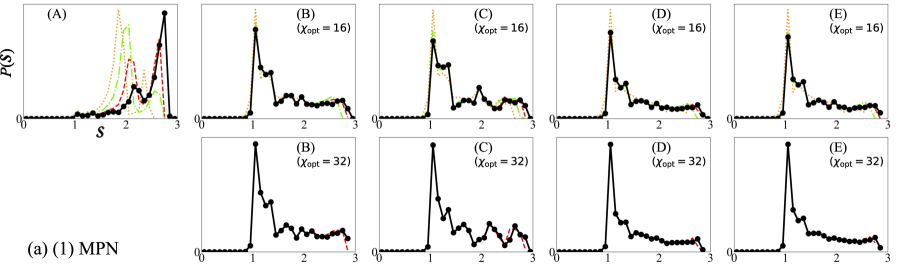
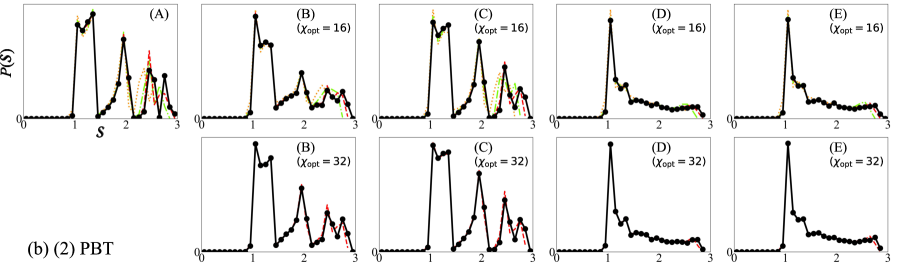
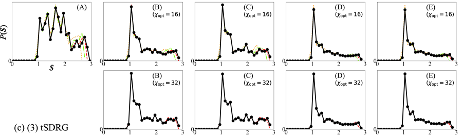
Figure 7: Histogram $P(\mathcal{S})$ of entanglement entropy $\mathcal{S}$ on auxiliary bonds in TTNs obtained by the types where the initial TTN is (a) (1) MPN, (b) (2) PBT, and (c) (3) TTN obtained by tSDRG, for $\mathcal{N}_{\rm s}=200$ random samples. Circles connected by solid lines represent the data at $\chi=40$. Dashed (red), dot-dashed (green), and dotted (orange) lines are the data at $\chi=32,24$, and $16$, respectively.

Those observations on the EEs are consistent with the findings obtained from the analyses of the variational energies. We thereby conclude that the stochastic structural optimizations [schemes (D) and (E)] work well for the random XY model and succeed in obtaining the best TTN structure yielding the lowest variational energy independently of the initial TTN.

III.3 Richardson Model

We have applied the TTN structural optimization algorithm to the Richardson model, that is a spin-1/2 model containing the all-to-all XY-exchange interactions under the magnetic field. The Hamiltonian is given by

$$\mathcal{H}_{\rm R}=\frac{J_{\rm R}}{N}\sum_{i=1}^{N-1}\sum_{j=i+1}^{N}(S^{x}_{i}S^{x}_{j}+S^{y}_{i}S^{y}_{j})-\sum_{i=1}^{N}h_{i}S^{z}_{i},$$ (14)

where $J_{\rm R}$ is the exchange-coupling parameter. The site-dependent longitudinal magnetic field is taken as

$$h_{i}=\frac{i-1}{N-1}-\frac{1}{2},$$ (15)

so that the field $h_{i}$ linearly increases from $h_{1}=-\frac{1}{2}$ to $h_{N}=\frac{1}{2}$ with increasing the site index $i$. The Richardson model [Eq. (14)] is known to be exactly solvable and has been studied for many years in condensed-matter physics, particularly in connection with the BCS superconductivity, and nuclear physics.[33, 34, 35]

As in the case of the random XY model in the previous section, we have performed several types of the structural optimization calculations to obtain the lowest-energy state in the subspace of zero total magnetization $\sum_{i}S^{z}_{i}=0$. The exchange constants and system sizes treated were $J_{\rm R}=1,4,16,64$ for $N=64$ and $J_{\rm R}=1$ for $N=128$. The maximum bond dimension treated was $\chi=80$. In the Richardson model, in which all spin pairs are coupled by the exchange interaction of the same strength, we can treat the system size $N$ and the bond dimension $\chi$ larger than those for the random XY model since we can carry out the calculation of exchange interaction terms with a much smaller (roughly speaking, $1/N$ times smaller) computational cost.

We performed the calculation of schemes (A) - (E) starting from the initial TTN of (1) MPN and (2) PBT. For schemes (B)-(E), the structural optimization was carried out at $\chi=\chi_{\rm opt}=20$ or $40$, and then, the calculation to optimize only the isometries was done with increasing $\chi$ up to 80. See Appendix B for the details. For stochastic schemes (D) and (E), we performed the calculations of four runs, i.e., two runs (with different random seeds) for each of the annealing parameters $(\beta_{0},n_{\tau})=(0.1,2)$ and $(0.1,4)$. In addition, in order to avoid the deadlock of the calculation due to isometry whose all three legs have dimension $\chi=1$ discussed in Sec. II, we adopted an exceptional treatment in the preparation process of the initial TTN. The details of the treatment are presented in Appendix A. In our calculations, the treatment was necessitated only for the cases where $(J_{\rm R},N)=(64,64)$ and the initial TTN was PBT.

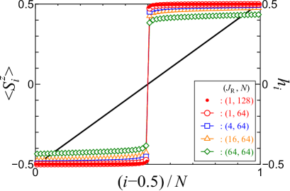
Figure 8: Local spin polarization $\langle S^{z}_{i}\rangle$. The plotted are the results obtained by the type which yields the smallest relative error $\delta e$ for each model parameter $(J_{\rm R},N)$. Thick black line represents the magnetic field $h_{i}$.

Before proceeding to the performance evaluation, let us examine the nature of the lowest energy state to be analyzed. In the Richardson model, the XY exchange interactions, which entangle all spins to form a large spin cluster, compete with the magnetic fields, which polarize the spins in the $S^{z}$ direction. Figure 8 presents the data of the spin polarization $\langle S^{z}_{i}\rangle$ in the lowest-energy states. For $J_{\rm R}=1$, when the exchange interaction is relatively weak, most of the spins except for those in the vicinity of $i=N/2$ are strongly polarized, $\langle S^{z}_{i}\rangle\sim\pm 1/2$, and almost classically ordered. Only the spins near $i=N/2$, where the field is weak, have the polarization slightly reduced by the exchange interactions; For example, $\langle S^{z}_{65}\rangle=-\langle S^{z}_{64}\rangle=0.4801$ for $J_{\rm R}=1$ and $N=128$. In this situation, the accuracy of the TTN calculation depends on how precisely the TTN state can represent the entanglement among those spins near $i=N/2$. As the exchange interaction $J_{\rm R}$ increases, the magnitude of the spin polarization decreases gradually, signaling that those spins start to entangle with each other to form a large spin cluster. A point to be noted here is that the $i$ dependence of the spin polarization remains flat except for the narrow region around $i=N/2$. Then, it is expected that the position in the TTN of those spins with nearly the same polarization does not affect the accuracy of the calculation very much. (Note that the exchange interactions take the same strength for all spin pairs and have no position dependence.) This point will be relevant in the later discussion on the TTN structure.

In order to discuss the accuracy of the TTN optimization quantitatively, we explore the relative error in the variational energies defined by

$$\delta e({\rm X},\chi) = \frac{E_{0}({\rm X},\chi)-E_{\rm exact}}{|E_{\rm exact}|},$$ (16)

$$\delta e^{\prime}({\rm X},\chi) = \frac{E^{\prime}_{0}({\rm X},\chi)-E_{\rm exact}}{|E_{\rm exact}|},$$ (17)

where $E_{\rm exact}$ is the exact lowest energy obtained from the exact solution of the Richardson model[33, 34, 35]; see Appendix C for the calculation of $E_{\rm exact}$. We will see that $\delta e$ and $\delta e^{\prime}$ exhibit qualitatively similar behavior, although $\delta e^{\prime}$ is by definition not less than $\delta e$. However, the difference between $\delta e$ and $\delta e^{\prime}$ is noticeable when the TTN is PBT [type (2A)]. This is because in PBT, the EE on the “top” bond is significantly larger than EEs on other bonds and $\delta e$ obtained at the top bond can avoid the effect of the truncation at the bond, which makes $\delta e$ lower than $\delta e^{\prime}$.

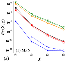
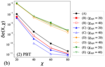
Figure 9: Relative error in the variational energy, $\delta e({\rm X},\chi)$, as functions of $\chi$, for the types where the initial TTN is (a) (1) MPN and (b) (2) PBT. The model parameters are $J_{\rm R}=1$ and $N=128$. For schemes (D) and (E), among the results of four runs, the ones of the run yielding the lowest variational energy at $\chi=80$ are plotted.

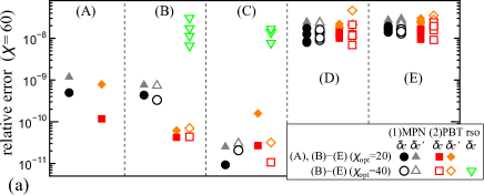
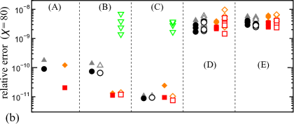
Figure 10: Relative errors in the variational energies, $\delta e({\rm X},\chi)$ and $\delta e^{\prime}({\rm X},\chi)$, at (a) $\chi=60$ and (b) $\chi=80$. The model parameters are $J_{\rm R}=1$ and $N=128$. Circles and squares (triangles and diamonds) represent $\delta e({\rm X},\chi)$ [$\delta e^{\prime}({\rm X},\chi)$] obtained by the types where the initial TTN is (1) MPN and (2) PBT, respectively. Solid symbols represent the results of (A) or (B)-(E) with $\chi_{\rm opt}=20$, while open symbols are those of (B)-(E) with $\chi_{\rm opt}=40$. For schemes (D) and (E), the results of four runs are plotted. Downward triangles represent $\delta e({\rm X},\chi)$ obtained by the calculations of schemes (B) and (C) with $\chi_{\rm opt}=40$ starting from PBTs with four different random site orderings (rso); see the main text. Some of the results for schemes (D) and (E) and the initial PBTs with random-site orderings overlap.

Let us compare $\delta e$ ($\delta e^{\prime}$) of various types of the calculation. Figure 9 shows the $\chi$ dependence of $\delta e({\rm X},\chi)$ for $(J_{\rm R},N)=(1,128)$. Also shown in Fig. 10 are the data of $\delta e({\rm X},\chi)$ and $\delta e^{\prime}({\rm X},\chi)$ for $\chi=60$ and $80$. We find that for the calculations with a fixed TTN structure [scheme (A)], PBT gives a rather accurate result. The non-stochastic optimization schemes [schemes (B) and (C)] yield results with better accuracy than those of scheme (A), except for (1B), whose accuracy is more or less the same as that of (1A). In particular, scheme (C) succeeded in realizing a sizable reduction of the relative error at $\chi=60$, compared to scheme (A) [see Fig. 10(a)]. The relative error $\delta e$ for (1C) with $\chi_{\rm opt}=20$ at $\chi=60$ and $80$ converge up to $\delta e(\chi=60)=9.3\times 10^{-12}$ and $\delta e(\chi=80)=8.8\times 10^{-12}$, indicating that the calculation gives a nearly exact result that reaches the accuracy limit of our TTN variational calculation (with double precision variables and the rule to discard the bases in isometry with singular values smaller than $10^{-6}$). These observations suggest that the non-stochastic structural optimization schemes are able to realize the accuracy improvement for the Richardson model, although the improvement may occasionally be small, like (1B) of the present case. On the other hand, the accuracy of the calculations of stochastic structural optimization [schemes (D) and (E)] is poor, even worse than that without structural optimization [scheme (A)], indicating that they do not work well for the Richardson model.

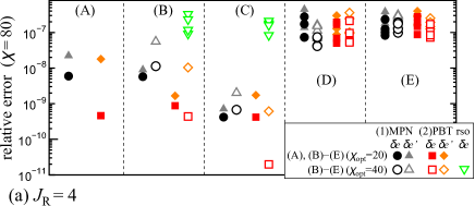
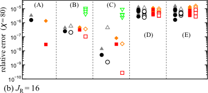
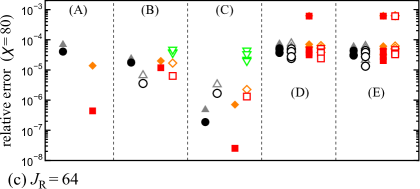
Figure 11: Relative errors in the variational energies, $\delta e({\rm X},\chi)$ and $\delta e^{\prime}({\rm X},\chi)$, at $\chi=80$ for $N=64$ and (a) $J_{\rm R}=4$, (b) $J_{\rm R}=16$, and (c) $J_{\rm R}=64$. Circles and squares (triangles and diamonds) represent $\delta e({\rm X},\chi)$ [$\delta e^{\prime}({\rm X},\chi)$] obtained by the types where the initial TTN is (1) MPN and (2) PBT, respectively. Solid symbols represent the data of (A) or (B)-(E) with $\chi_{\rm opt}=20$, while open symbols are those of (B)-(E) with $\chi_{\rm opt}=40$. For schemes (D) and (E), the results of four runs are plotted. Downward triangles represent $\delta e({\rm X},\chi)$ obtained by the calculations of schemes (B) and (C) with $\chi_{\rm opt}=40$ starting from PBTs with four different random site orderings (rso); see the main text. Some of the results for schemes (D) and (E) and the initial PBTs with random-site orderings overlap.

In Fig. 11, we show the results of $\delta e$ and $\delta e^{\prime}$ for $J_{\rm R}=4,16,64$ and $N=64$. These data for large $J_{\rm R}$ also indicate basically the same results as those for $J_{\rm R}=1$. That is, when the initial TTN is MPN, the non-stochastic optimization [schemes (B) and (C)] may achieve accuracy improvement, although the calculation is occasionally stuck in a state of poor accuracy. PBT yields a result with good accuracy as it is, but even better accuracy may be achieved by the calculation of scheme (C). In contrast, the calculations of stochastic schemes (D) and (E) are not accurate and do not work well for the Richardson model.

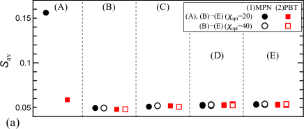
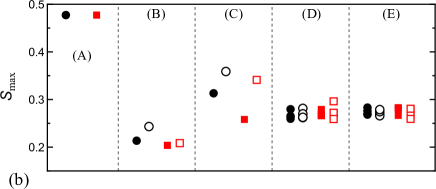
Figure 12: (a) Average value $\mathcal{S}_{\rm av}$ and (b) maximum value $\mathcal{S}_{\rm max}$ of EEs on auxiliary bonds for $J_{\rm R}=1$ and $N=128$. Circles and squares represent the data at $\chi=80$ of the types where the initial TTN is (1) MPN and (2) PBT, respectively. Solid symbols represent the data of (A) or (B)-(E) with $\chi_{\rm opt}=20$, while open symbols are those of (B)-(E) with $\chi_{\rm opt}=40$. For schemes (D) and (E), the results of four runs are plotted. The $\chi$ convergence is confirmed by comparing the results at $\chi=80$ and $60$. Some of the results for schemes (D) and (E) overlap.

Figure 12 shows the average and maximum values of the EE on auxiliary bonds, $\mathcal{S}_{\rm av}$ and $\mathcal{S}_{\rm max}$, for $J_{\rm R}=1$ and $N=128$. The average value $\mathcal{S}_{\rm av}$ is remarkably large for (1A), where the TTN structure is fixed to be MPN, while $\mathcal{S}_{\rm av}$ for the other types are small. The maximum values $\mathcal{S}_{\rm max}$ for (1A) and (2A), where the TTN structures are MPN and PBT, are the same and large, which are the values on the bond corresponding to the bipartition of the system into two parts of $1\leq i\leq N/2$ and $N/2+1\leq i\leq N$. $\mathcal{S}_{\rm max}$ for other types are smaller than those of (1A) and (2A); in particular, scheme (B) yields the smallest $\mathcal{S}_{\rm max}$, indicating that scheme (B), which directly uses the EE as a measure in selecting the local TTN structure, is the most suitable for minimizing the maximum value of EE. The qualitatively same features of $\mathcal{S}_{\rm av}$ and $\mathcal{S}_{\rm max}$ are also observed for other model parameters $J_{\rm R}$ and $N$ (data not shown), while the values of $\mathcal{S}_{\rm av}$ and $\mathcal{S}_{\rm max}$ increase with $J_{\rm R}$. Here, we recall that the relative errors in the variational energy were smallest for scheme (C) in most cases. These results thus suggest that there was no strong correlation between the accuracy of the variational energy and the average and maximum EEs in the Richardson model. The observations indicate the importance of choosing the adequate scheme of the network optimization depending on the model treated and the quantity to be minimized.

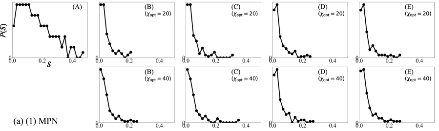
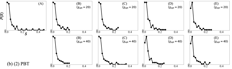
Figure 13: Histogram $P(\mathcal{S})$ of entanglement entropy $\mathcal{S}$ on auxiliary bonds in TTNs obtained by the types where the initial TTN is (a) (1) MPN and (b) (2) PBT for $J_{\rm R}=1$ and $N=128$. Circles connected by solid lines represent the data at $\chi=80$. The $\chi$ convergence is confirmed by comparing the results at $\chi=80$ and $60$. The size of bins is set to be $\Delta\mathcal{S}=0.02$. For schemes (D) and (E), among the results of four runs, the one obtained by the run yielding the lowest variational energy at $\chi=80$ is plotted.

The histograms of EEs on auxilialy bonds for $(J_{\rm R},N)=(1,128)$ are shown in Fig. 13. The bin size is set to be $\Delta\mathcal{S}=0.02$. We find that only the histogram of type (1A), which uses the TTN structure fixed to MPN, exhibits a slowly decreasing behavior that is different from the other types. The histograms except the one of (1A) show a similar structure in which the frequency takes the largest value at a small EE and rapidly decreases as the EE increases. The histograms for the other values of $J_{\rm R}$ and $N$ (not shown here) exhibit qualitatively the same behavior, while the scale of the horizontal axis (the values of EE) increases with $J_{\rm R}$. It is thus suggested that in the Richardson model, the histograms of EE also have no strong correlation with the accuracy in the variational enegy.

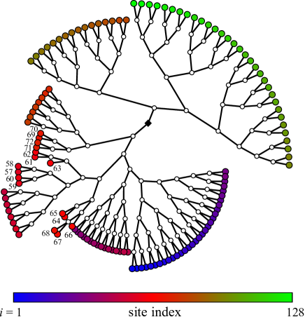
Figure 14: TTN structure obtained by type (2C) with $\chi_{\rm opt}=40$, which yielded the lowest variational energy at $\chi=80$, for $J_{\rm R}=1$ and $N=128$. Open circles represent isometries and the solid diamond represents the singular-value matrix. Bare spins are represented by circles with colors varying according to the site index $i$ as shown in the color bar. Bare spins with the site index $57\leq i\leq 72$ are indicated by numbers.

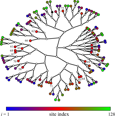
Figure 15: TTN structure obtained by a calculation of type (2D) with $\chi_{\rm opt}=40$, which yielded a high vatiational energy, for $J_{\rm R}=1$ and $N=128$. Open circles represent isometries and the solid diamond represents the singular-value matrix. Bare spins are represented by circles with colors varying according to the site index $i$ as shown in the color bar. Bare spins with the site index $57\leq i\leq 72$ are indicated by numbers.

Finally, we examine the TTN structure obtained. As discussed above, the optimal TTN for the Richardson model with Eq. (15) is expected to have a structure suitable for representing the entanglement among quantum-fluctuating spins around $i=N/2$. Figure 14 presents the TTN structure obtained by the calculation of type (2C) with $\chi_{\rm opt}=40$ for $J_{\rm R}=1$ and $N=128$, which yielded the lowest variational energy. In this TTN, the spins around $i=N/2$ are located close to each other, indicating that a structure nearly the optimal one is realized by the calculation. (To be precise, as the spins at the sites $69\leq i\leq 72$ are not far away but slightly apart from the clusters of the spins at $57\leq i\leq 68$ in the TTN obtained, the TTN should not be the “truly optimal”, although it is close enough to the optimal to yield the lowest variational energy.) Note that in the initial PBT of the present calculation, the spins around $i=N/2$ are separated into the two groups of $i\leq N/2$ and $i\geq N/2+1$, which are located far apart; therefore, the initial PBT is not suitable for representing the entanglement between the groups, although entanglement among the spins within each group can be taken into account well. Our algorithm achieves a structural change from the initial PBT to the nearly optimal TTN. We have also confirmed that the TTNs with the smallest variational energy obtained for other model parameters, $J_{\rm R}=1,4,16,64$ and $N=64$ have the similar structure in which the spins near $i=N/2$ are clustered close together, as in Fig. 14.

The result that the stochastic schemes do not work well for the Richardson model also manifests itself in the TTN structure. Figure 15 shows the TTN structure obtained by a calculation of type (2D) with $\chi_{\rm opt}=40$ for $J_{\rm R}=1$ and $N=128$, which yielded a relatively high energy. In this TTN, the spins around $i=N/2$ are scattered into various branches, and the TTN should be unsuitable for expressing the entanglement among those spins. The reason why the stochastic scheme obtained such a TTN may be understood as follows. Roughly speaking, in stochastic schemes, the TTN structure is randomized by probabilistic selection of local TTN structures at the early stage of the calculation where the effective temperature is high, which scatters the spins around $i=N/2$ into various branches. Then, the TTN structure is optimized as the effective temperature is lowered. However, in the randomized TTN, the spins near $i=N/2$ are surrounded by nearly classical-ordered spins at the sites away from $i=N/2$. In the process of local reconnection of isometries in the structural optimization, the position swap of the blocks consisting of such classically ordered spins does not change the EE or truncated rDM weight at the center bond very much. As a result, the “slope” of the cost function of EE or truncated rDM weight in the TTN-structural space becomes small in such a TTN, which slows down the structural optimization and makes it easier to be trapped even in a shallow local minimum. This situation may not change even if $J_{\rm R}$ becomes larger, as long as the profile of $\langle S^{z}_{i}\rangle$ is flat and the effect of local reconnection of isometries on the cost function is small. Thus, the poor accuracy of the stochastic schemes may be attributed to the fact that those schemes create an effective initial TTN structure where the slope of cost function in the local structural update is small and the optimization flow slows down and even freezes.

To confirm the above scenario, we performed four runs of the calculations of non-stochastic schemes [schemes (B) and (C)] with $\chi_{\rm opt}=40$, starting from a PBT in which the bare spins are arranged randomly. The relative error in the variational energy, $\delta e$, obtained are shown in Figs. 10 and 11 (by downward triangles). The results indicate that the accuracy of the calculation is as poor as that of stochastic schemes [schemes (D) and (E)], supporting the above scenario that the stochastic optimization is roughly equivalent to the non-stochstic one starting from a randomized TTN. These observations underscore the importance of appropriately selecting the initial TTN as well as the optimization scheme according to the system treated.

In non-stochastic schemes (B) and (C), there are some cases where the relative error in the variational energy is large, as seen in Figs. 10 and 11. This may also be caused by the phenomenon that once the structural optimization flow strays into the TTN structure with a small slope of the cost function, it is stuck there.

IV Concluding Remarks

In summary, we have evaluated the performance of the TTN structural optimization algorithm for variational calculations of quantum many-body systems. We have examined several types of the algorithm, which are specified by the initial TTN structure, the scheme to update the local connection of isometries in the structural optimization, and the bond dimention at which the structural optimization is performed. We applied them to the random XY-exchange model under random magnetic field and the Richardson model and analyzed the variational energies and the EEs on the auxiliary bonds. The results for the random XY model, on the one hand, demonstrate that the TTN structural optimization algorithm works effectively to improve the accuracy of the calculation for the model. In particular, we have found that stochastic schemes, which probabilistically select the local connection of isometries in the optimization process, yield the best results in the random average of the variational energy, regardless of the initial TTN structure. For the Richardson model, on the other hand, the results show that the structural optimization algorithm of an appropriately selected type can realize a lower variational energy than those obtained by the calculation without TTN structural optimization. Nevertheless, we have also found that, particularly in the calculations of stochastic schemes, the TTN structure obtained by the optimization can stuck in a structure that is not suitable for representing the lowest energy state of interest, resulting in poor calculation accuracy. This indicates the importance of appropriately choosing the initial TTN structure as well as the schemes of selecting local connections of isometries in the structural optimization, depending on the model.

The TTN structural optimization algorithm we proposed searches for the optimal structure through local reconnections of the network. Therefore, it is essential to devise a way to realize fast and steady convergence to the optimal structure. We have tested the stochastic schemes according to Eqs. (5) and (6). For the random XY model, the stochastic schemes succeeded in obtaining the lowest variational energies independent of the initial TTN structure, while non-stochastic schemes yielded results that are good but not the best and depend on the initial TTN. In the random XY model, the landscape of variational energy in the TTN-structure space is expected to be complex, and the optimization flow of the non-stochastic scheme is likely to be trapped in local minima, leading to an increase in the variational energy. The stochastic scheme should be effective in promoting the escape from such local minima. In contrast, for the Richardson model, the stochastic schemes yielded high variational energies, while the non-stochastic schemes achieved relatively good results depending on the initial TTN. A possible explanation for this result is that once the TTN structure is randomized at the early stage of stochastic optimization, the slope of EE in the TTN structural space almost vanishes, and the optimization flow can be easily trapped in a shallow minimum. In order to avoid the problem, it may be effective to try multiple calculations from various initial TTNs as well as to adjust the annealing schedule in the stochastic optimization. The idea of the replica exchange method[36, 37], which has recently been applied to the structural optimization of tensor networks with loops[38], is also expected to be promising.

While we focused in this work on the performance of the TTN structural optimization algorithm in the variational calculation of quantum many-body systems, it has many other potential applications. One promising application is the one to an efficient representation of a given high-rank tensor in the TTN format. In the algorithm we proposed, each step involves the diagonalization of the effective Hamiltonian expanded in the truncated Hilbert space of the central area to obtain the ground-state wave function (process 3 of Table 1). By replacing this process with the one to obtain a wave function that has a maximum fidelity to the given high-rank tensor, one can optimize only the TTN structure without changing the TTN state itself.[39] Such an application is expected to be useful for machine learning[40, 41] and quantics tensor-train approach[42, 43, 44], to which tensor networks have been applied actively in recent years. An application of a similar algorithm using bond mutual information as a cost function to the Born machine has been explored very recently.[45]

Appendix A Preparation of initial TTN

In our calculation, isometries in the initial TTN are prepared as follows. For example, let us consider the MPN shown in Fig. 1 (a). First, we focus on the subsystem consisting of the leftmost two spins at the sites $i=1$ and $2$ in the MPN and construct its block Hamiltonian. Then, we generate the leftmost isometry using the $\chi$ eigenvectors of the block Hamiltonian with the $\chi$-lowest eigenenergies. If the number of eigenvectors of the block Hamiltonian does not exceed $\chi$, all eigenvectors are adopted in the isometry. Next, we focus on the subsystem consisting of the leftmost two-site block and the neighboring spin at the site $i=3$, construct and diagonalize the block Hamiltonian of the subsystem, and generate the new isometry using the $\chi$-lowest-energy eigenvectors. We iterate these procedures from the left edge to the center of the MPN, where the canonical center is located, and perform the same operation from the right edge to the center to eventually prepare the initial MPN. (To be precise, we generate only the isometries in the initial TTN and not the singular-value matrix, the latter not necessary for the start of our calculation.) The other initial TTNs are also prepared in the same way, with the only difference being that we change the order of merging the spin blocks. In the case of PBT, the spin blocks are merged from the boundary of PBT, where the bare spins are located, to the “top” of PBT, where the canonical center is, so that PBT shown in Fig. 1 (b) is constructed. In the case of the tSDRG, in each step of the preparation procedure, we construct the interaction Hamiltonians of all the pairs of spin blocks, diagonalize them, and calculate the maximum level spacing $\Delta_{\rm max}^{\rm I}$ of their energy spectrum. Then, among all the spin-block pairs, we select the one with the largest $\Delta_{\rm max}^{\rm I}$ to be merged at the step. See Ref. [29] for the details.

In general, in our algorithm, the structure of the initial TTN can be arbitrary. The closer the structure of the initial TTN is to the optimal one, the faster the convergence of the calculation is. As for the initial isometries, any isometries can be used as long as they satisfy the orthonormal condition Eq. (1). Preparing the isometries using random vectors satisfying the condition may be a reasonable choice. It is also possible to use a product state, a TTN with $\chi=1$, as the initial TTN. However, in that case, it is necessary to take measures against the problem of the appearance of an isometry whose three legs have the dimension unity, mentioned in Sec. II, since the TTN with $\chi=1$ of a generic structure inevitably contains such an isometry and the calculation will be stuck. A possible measure to avoid the problem is employing a MPN as the structure of the initial TTN so that the central area has at least two physical bonds, whose dimension is usually larger than unity, as the incoming bonds, and increasing the dimension of auxiliary bonds sufficiently before starting the structural optimization.

The problem of the isometry having three legs of the dimension unity may also occur accidentally during the TTN optimization calculation. In our calculations of the present work, we encountered the problem in several cases of the calculation of the types where the initial TTN was (2) PBT for the Richardson model with $(J_{\rm R},N)=(64,64)$, if we did not take the exceptional treatment mentioned below. The problem occurred when the initial PBT included isometries whose outgoing bond was composed of the $\chi$-lowest-energy eigenstates of the block Hamiltonian all of which belonged to the subspace of the same magnetization. Since the states of the spin block represented by such an isometry can take only the single magnetization in the truncated Hilbert space, the XY-exchange interactions between the block and the rest of the system become zero, and the block is decoupled. Then, if two or more such blocks are connected to the central area at a step in the TTN calculation, the rank of the ground-state wave function in one (or more) singular-value decomposition becomes unity, generating a bond with dimension $\chi=1$. The cumulation of such a process may result in the emergence of the isometry with all three legs having the dimension $\chi=1$.

In order to avoid such a situation, for the Richardson model, we adopted an exceptional treatment in the procedure to prepare the initial PBT; Namely, if all of the $\chi$-lowest-energy eigenstates of the block Hamiltonian had the same magnetization, we discarded the state with the highest energy (or the highest-energy multiplet if the states were degenerate) and incorporated the lowest-energy state in the subspaces with the one higher and one lower magnetization to construct the isometry. We succeeded in avoiding the problem with this treatment.

Appendix B Details of calculations

In our TTN calculations, we computed physical quantities such as variational energies as a function of the upper bound of the bond dimension, $\chi$, with increasing $\chi$. The calculations for the random XY model and the Richardson model were performed in the following manner.

random XY model: For the calculation without structural optimization [scheme (A)], we performed the variational calculation to optimize the isometries with increasing $\chi$ as $\chi=16(100),24(20),32(20),40(20)$, where the figures in the parentheses are the maximum number of sweeps iterated at each $\chi$. If the variational energy converged within the range of $10^{-5}$ before the maximum number of sweeps was reached, we finished the calculation at the value of $\chi$ and proceeded to the next $\chi$. We then adopted the lowest variational energy obtained during the sweeps as the variational energy for each $\chi$.

For the calculations with the structural optimization [schemes (B)-(E)], we first performed the calculations with the structural-optimization procedure with $\chi=\chi_{\rm opt}$; two cases of calculations with $\chi_{\rm opt}=16$ and $32$ were carried out. We iterated the structural-optimization calculations until the TTN structure and the variational energy converged, and then adopted the TTN structure obtained as the optimized one in the following calculation. If the calculation did not converge within $80$ sweeps, the TTN structure obtained after the last sweep was used as the optimized one. After the optimized TTN structure was determined, we performed the variational calculation to optimize the isometries with increasing $\chi$ as $\chi=16,24,32,40$ for $\chi_{\rm opt}=16$ and $\chi=32,40$ for $\chi_{\rm opt}=32$. The calculation at each $\chi$ was continued until the variational energy converged or the number of sweeps reached $20$.

Richardson model: The calculations for the Richardson model were performed basically in the same manner as for the random XY model, with slight differences (see below).

For the calculation without structural optimization, we performed the calculation to optimize the isometries with increasing $\chi$ as $\chi=20(100),40(20),60(20),80(20)$, where the figures in the parentheses denote the number of sweeps iterated at each $\chi$. Here, differently from the case of the random XY model, we did not monitor the convergence of the variational energy but instead performed the calculation of the stated number of sweeps. We then adopted the lowest variational energy obtained during the sweeps as the variational energy at the value of $\chi$. For the calculations with the structural optimization, we performed the calculations with the structural-optimization procedure with $\chi=\chi_{\rm opt}=20$ or $40$ until the convergence of the TTN structure and the variational energy (within the range of $10^{-6}$) was achieved or the number of sweeps reached $80$. After that, we performed the variational calculation to optimize the isometries with increasing $\chi$ as $\chi=20,40,60,80$ for $\chi_{\rm opt}=20$ and $\chi=40,60,80$ for $\chi_{\rm opt}=40$. We iterated the calculations of 20 sweeps for each $\chi$ to obtain the variational energy as a function of $\chi$.

Appendix C Exact solution of Richardson model

The Richardson model given by Eq. (14) is exactly solvable. We calculated the exact ground-state energy of the model using the equations and method summarized below. Here, we assume that the magnetic fields $\{h_{i}\}$ are non-degenerate. We refer the readers to Ref. [33] for more details.

First, we rewrite the spin Hamiltonian $\mathcal{H}_{\rm R}$ in Eq. (14) in terms of hardcore bosons. The spin-1/2 operators can be represented using the hardcore boson operators as

$$S^{+}_{i}=b_{i},~~~S^{-}_{i}=b_{i}^{\dagger},~~~S^{z}_{i}=\frac{1}{2}-b_{i}^{\dagger}b_{i},$$ (18)

where $S^{\pm}_{i}=S^{x}_{i}\pm iS^{y}_{i}$, and $b_{i}$ is the hardcore-boson operator at $i$ th site obeying $\left[b_{i},b_{i^{\prime}}^{\dagger}\right]=\left(1-2b_{i}^{\dagger}b_{i}\right)\delta_{ii^{\prime}}$ and $\left(b_{i}^{\dagger}\right)^{2}=0$. Substituting the expressions of Eq. (18) into the spin Hamiltonian $\mathcal{H}_{\rm R}$, one can map the spin model into the interacting hardcore-boson model $\tilde{\mathcal{H}}_{\rm R}$ as

$$\mathcal{H}_{\rm R} = \tilde{\mathcal{H}}_{\rm R}-\frac{1}{2}\sum_{i=1}^{N}h_{i}+gN_{\rm b},$$ (19)

$$\tilde{\mathcal{H}}_{\rm R} = \sum_{i=1}^{N}\sum_{i^{\prime}=1}^{N}\left(h_{i}\delta_{ii^{\prime}}-g\right)b^{\dagger}_{i}b_{i^{\prime}}.$$ (20)

The coupling constant $g$ and the number of hardcore bosons, $N_{\rm b}$, are respectively given by

$$g = -\frac{J_{\rm R}}{2N},$$ (21)

$$N_{\rm b} = \frac{N}{2}-M,$$ (22)

where $M=\sum_{i=1}^{N}S^{z}_{i}$ is the total magnetization. We consider the case of even $N_{\rm b}$ in the following.

The eigenstates of the Hamiltonian $\tilde{\mathcal{H}}_{\rm R}$ [Eq. (20)] can be written down explicitly as

$$|\tilde{\Psi}_{\rm R}\rangle = \prod_{n=1}^{N_{\rm b}}B^{\dagger}_{n}|0\rangle,$$ (23)

$$B^{\dagger}_{n} = \sum_{i=1}^{N}\frac{b^{\dagger}_{i}}{h_{i}-E_{n}},$$ (24)

where $|0\rangle$ is the vacuum of the bosons $\{b_{i}\}$. The state $|\tilde{\Psi}_{\rm R}\rangle$ in Eq. (23) is an exact eigenstate of the Hamiltonian $\tilde{\mathcal{H}}_{\rm R}$ if the parameters $\{E_{n}\}$ satisfy the coupled equations,

$$1-\sum_{i=1}^{N}\frac{g}{h_{i}-E_{n}}+\sum_{n^{\prime}=1(\neq n)}^{N_{\rm b}}\frac{2g}{E_{n^{\prime}}-E_{n}}=0,$$ (25)

for $n=1,...,N_{\rm b}$. The eigenenergy is obtained as

$$\mathcal{E}=\sum_{n=1}^{N_{\rm b}}E_{n}.$$ (26)

The solution $\{E_{n}\}$ of the coupled equations (25) consists of real numbers or complex conjugate pairs. We thus express $\{E_{n}\}$ as

$$E_{2p-1}=x_{p}-iy_{p},~~~E_{2p}=x_{p}+iy_{p},$$ (27)

for $p=1,...,N_{\rm b}/2$, where $x_{p}$ are real and $y_{p}$ are real or pure imaginary. The coupled equations (25) are rewritten as

$$1-g\sum_{i=1}^{N}\frac{h_{i}-x_{p}}{(h_{i}-x_{p})^{2}+y_{p}^{2}}$$

$$~~+4g\sum_{p^{\prime}=1(\neq p)}^{N_{\rm b}/2}\frac{(x_{p^{\prime}}-x_{p})\left[(x_{p^{\prime}}-x_{p})^{2}+y_{p}^{2}+y_{p^{\prime}}^{2}\right]}{\left[(x_{p^{\prime}}-x_{p})^{2}+y_{p}^{2}+y_{p^{\prime}}^{2}\right]^{2}-4y_{p}^{2}y_{p^{\prime}}^{2}}=0,$$

(28)

$$1-\sum_{i=1}^{N}\frac{y_{p}^{2}}{(h_{i}-x_{p})^{2}+y_{p}^{2}}$$

$$~~+4\sum_{p^{\prime}=1(\neq p)}^{N_{\rm b}/2}\frac{y_{p}^{2}\left[(x_{p^{\prime}}-x_{p})^{2}+y_{p}^{2}+y_{p^{\prime}}^{2}\right]-2y_{p}^{2}y_{p^{\prime}}^{2}}{\left[(x_{p^{\prime}}-x_{p})^{2}+y_{p}^{2}+y_{p^{\prime}}^{2}\right]^{2}-4y_{p}^{2}y_{p^{\prime}}^{2}}=0.$$

(29)

Note that in these equations, $y_{p}$ appears only in the form of $y_{p}^{2}$. We thus treat $\{x_{p}\}$ and $\{y_{p}^{2}\}$ as real parameters and solve the coupled equations (28) and (29) numerically using the Newton-Raphson method[46].

It should be noted that the above coupled equations may yield not only the ground state but also an arbitrary eigenstate of the Richardson model. We obtained the ground-state solution in the following manner. First, the ground-state solution at $g=0$ is trivially obtained as

$$E_{n}(g=0)=h_{n},~~(n=1,...,N_{\rm b})$$ (30)

or equivalently,

$$x_{p}(g=0) = \frac{h_{2p}+h_{2p-1}}{2},$$ (31)

$$y_{p}^{2}(g=0) = -\left(\frac{h_{2p}-h_{2p-1}}{2}\right)^{2}.$$ (32)

Here, note that the field $h_{i}$ is arranged in the ascending order. Furthermore, for $g=-\delta g$ with a small $\delta g>0$, the approximate ground-state solution up to the first order of $\delta g$ is obtained as

$$\bar{x}_{p}(g=-\delta g) = \frac{h_{2p}+h_{2p-1}}{2}+\delta g,$$ (33)

$$\bar{y}_{p}^{2}(g=-\delta g) = -\left(\frac{h_{2p}-h_{2p-1}}{2}\right)^{2}.$$ (34)

We adopted these values as initial guesses and input them into the Newton-Raphson method to obtain the ground-state solution for $g=-\delta g$. Afterwards, we prepared the initial guesses for $g=-n~\delta g$ ($n=2,3,4,...$) as

$$\bar{x}_{p}(g=-n~\delta g) = 2x_{p}(g=-(n-1)\delta g)$$ (35)

$$-x_{p}(g=-(n-2)\delta g),$$

$$\bar{y}_{p}^{2}(g=-n~\delta g) = 2y_{p}^{2}(g=-(n-1)\delta g)$$ (36)

$$-y_{p}^{2}(g=-(n-2)\delta g),$$

and input them into the Newton-Raphson method. In such a manner, we obtained the ground-state solutions as a function of $g$ with decreasing $g$ [increasing $J_{\rm R}$ in Eq. (21)] adiabatically. The obtained ground-state energies for the model parameters discussed in Sec. III.3 are presented in Table 2.

Table 2: Exact ground-state energy of the Richardson model [Eq. (14)] with the magnetic field term of Eq. (15) for the model parameters $(J_{\rm R},N)=(1.0,64),(4.0,64),(16.0,64),(64.0,64)$, and $(1.0,128)$.

$J_{\rm R}$	$N$	$E_{\rm ex}$
1.0	64	-8.20139294258928
4.0	64	-8.64996248818904(1)
16.0	64	-11.00530807225508
64.0	64	-21.76617777856154(1)
1.0	128	-16.20027338853789

References

- White [1992] S. R. White, Density matrix formulation for quantum renormalization groups, Phys. Rev. Lett. 69, 2863 (1992).
- White [1993] S. R. White, Density-matrix algorithms for quantum renormalization groups, Phys. Rev. B 48, 10345 (1993).
- Orús [2019] R. Orús, Tensor networks for complex quantum systems, Nature Reviews Physics 1, 538 (2019).
- Okunishi et al. [2022] K. Okunishi, T. Nishino, and H. Ueda, Developments in the tensor network - from statistical mechanics to quantum entanglement, Journal of the Physical Society of Japan 91, 062001 (2022).
- Larsson [2024] H. R. Larsson, A tensor network view of multilayer multiconfiguration time-dependent hartree methods, Molecular Physics 0, e2306881 (2024), https://doi.org/10.1080/00268976.2024.2306881 .
- Baxter [1968] R. J. Baxter, Dimers on a rectangular lattice, J. Math. Phys 9, 650 (1968).
- Östlund and Rommer [1995] S. Östlund and S. Rommer, Thermodynamic limit of density matrix renormalization, Phys. Rev. Lett. 75, 3537 (1995).
- Rommer and Östlund [1997] S. Rommer and S. Östlund, Class of ansatz wave functions for one-dimensional spin systems and their relation to the density matrix renormalization group, Phys. Rev. B 55, 2164 (1997).
- Nishino et al. [2001] T. Nishino, Y. Hieida, K. Okunishi, N. Maeshima, Y. Akutsu, and A. Gendiar, Two-Dimensional Tensor Product Variational Formulation, Prog. Theor. Phys. 105, 409 (2001).
- Gendiar et al. [2003] A. Gendiar, N. Maeshima, and T. Nishino, Stable Optimization of a Tensor Product Variational State, Prog. Theor. Phys. 110, 691 (2003).
- Verstraete and Cirac [2004] F. Verstraete and J. I. Cirac, Valence-bond states for quantum computation, Phys. Rev. A 70, 060302 (2004).
- Verstraete et al. [2006] F. Verstraete, M. M. Wolf, D. Pérez-García, and J. I. Cirac, Criticality, the area law, and the computational power of projected entangled pair states, Phys. Rev. Lett. 96, 220601 (2006).
- Vidal [2007] G. Vidal, Entanglement renormalization, Phys. Rev. Lett. 99, 220405 (2007).
- Evenbly and Vidal [2009] G. Evenbly and G. Vidal, Algorithms for entanglement renormalization, Phys. Rev. B 79, 144108 (2009).
- Seki et al. [2021] K. Seki, T. Hikihara, and K. Okunishi, Entanglement-based tensor-network strong-disorder renormalization group, Phys. Rev. B 104, 134405 (2021).
- Hikihara et al. [2023] T. Hikihara, H. Ueda, K. Okunishi, K. Harada, and T. Nishino, Automatic structural optimization of tree tensor networks, Phys. Rev. Res. 5, 013031 (2023).
- Okunishi et al. [2023] K. Okunishi, H. Ueda, and T. Nishino, Entanglement bipartitioning and tree tensor networks, Progress of Theoretical and Experimental Physics 2023, 023A02 (2023), https://academic.oup.com/ptep/article-pdf/2023/2/023A02/49294184/ptad018.pdf .
- Chan and Head-Gordon [2002] G. K.-L. Chan and M. Head-Gordon, Highly correlated calculations with a polynomial cost algorithm: A study of the density matrix renormalization group, The Journal of Chemical Physics 116, 4462 (2002), https://pubs.aip.org/aip/jcp/article-pdf/116/11/4462/19222618/4462_1_online.pdf .
- Legeza and Sólyom [2003] O. Legeza and J. Sólyom, Optimizing the density-matrix renormalization group method using quantum information entropy, Phys. Rev. B 68, 195116 (2003).
- Moritz et al. [2004] G. Moritz, B. A. Hess, and M. Reiher, Convergence behavior of the density-matrix renormalization group algorithm for optimized orbital orderings, The Journal of Chemical Physics 122, 024107 (2004), https://pubs.aip.org/aip/jcp/article-pdf/doi/10.1063/1.1824891/10872404/024107_1_online.pdf .
- Legeza et al. [2015] O. Legeza, L. Veis, A. Poves, and J. Dukelsky, Advanced density matrix renormalization group method for nuclear structure calculations, Phys. Rev. C 92, 051303 (2015).
- Li et al. [2022] W. Li, J. Ren, H. Yang, and Z. Shuai, On the fly swapping algorithm for ordering of degrees of freedom in density matrix renormalization group, Journal of Physics: Condensed Matter 34, 254003 (2022).
- Larsson [2019] H. R. Larsson, Computing vibrational eigenstates with tree tensor network states (ttns), The Journal of Chemical Physics 151, 204102 (2019), https://doi.org/10.1063/1.5130390 .
- Ma et al. [1979] S.-k. Ma, C. Dasgupta, and C.-k. Hu, Random antiferromagnetic chain, Phys. Rev. Lett. 43, 1434 (1979).
- Dasgupta and Ma [1980] C. Dasgupta and S.-k. Ma, Low-temperature properties of the random heisenberg antiferromagnetic chain, Phys. Rev. B 22, 1305 (1980).
- Hikihara et al. [1999] T. Hikihara, A. Furusaki, and M. Sigrist, Numerical renormalization-group study of spin correlations in one-dimensional random spin chains, Phys. Rev. B 60, 12116 (1999).
- Goldsborough and Römer [2014] A. M. Goldsborough and R. A. Römer, Self-assembling tensor networks and holography in disordered spin chains, Phys. Rev. B 89, 214203 (2014).
- Lin et al. [2017] Y.-P. Lin, Y.-J. Kao, P. Chen, and Y.-C. Lin, Griffiths singularities in the random quantum ising antiferromagnet: A tree tensor network renormalization group study, Phys. Rev. B 96, 064427 (2017).
- Seki et al. [2020] K. Seki, T. Hikihara, and K. Okunishi, Tensor-network strong-disorder renormalization groups for random quantum spin systems in two dimensions, Phys. Rev. B 102, 144439 (2020).
- Hikihara et al. [2024] T. Hikihara, H. Ueda, K. Okunishi, K. Harada, and T. Nishino, Visualization of entanglement geometry by structural optimization of tree tensor network (2024), arXiv:2401.16000 [cond-mat.stat-mech] .
- Shi et al. [2006] Y.-Y. Shi, L.-M. Duan, and G. Vidal, Classical simulation of quantum many-body systems with a tree tensor network, Phys. Rev. A 74, 022320 (2006).
- [32] In the actual computation, one of the two isometries will be included in the central area in the next step and does not necessarily need to be updated.
- von Delft and Ralph [2001] J. von Delft and D. Ralph, Spectroscopy of discrete energy levels in ultrasmall metallic grains, Physics Reports 345, 61 (2001).
- Asorey et al. [2002] M. Asorey, F. Falceto, and G. Sierra, Chern-simons theory and bcs superconductivity, Nuclear Physics B 622, 593 (2002).
- Dukelsky et al. [2004] J. Dukelsky, S. Pittel, and G. Sierra, Colloquium: Exactly solvable richardson-gaudin models for many-body quantum systems, Rev. Mod. Phys. 76, 643 (2004).
- Hukushima and Nemoto [1996] K. Hukushima and K. Nemoto, Exchange monte carlo method and application to spin glass simulations, Journal of the Physical Society of Japan 65, 1604 (1996), https://doi.org/10.1143/JPSJ.65.1604 .
- Rozada et al. [2019] I. Rozada, M. Aramon, J. Machta, and H. G. Katzgraber, Effects of setting temperatures in the parallel tempering monte carlo algorithm, Phys. Rev. E 100, 043311 (2019).
- Watanabe and Ueda [2024] R. Watanabe and H. Ueda, Automatic structural search of tensor network states including entanglement renormalization, Phys. Rev. Res. 6, 033259 (2024).
- [39] R. Watanabe, H. Manabe, T. Hikihara, and H. Ueda, in preparation.
- Stoudenmire and Schwab [2016] E. Stoudenmire and D. J. Schwab, Supervised learning with tensor networks, in Advances in Neural Information Processing Systems, Vol. 29, edited by D. Lee, M. Sugiyama, U. Luxburg, I. Guyon, and R. Garnett (Curran Associates, Inc., 2016).
- Cheng et al. [2019] S. Cheng, L. Wang, T. Xiang, and P. Zhang, Tree tensor networks for generative modeling, Phys. Rev. B 99, 155131 (2019).
- Shinaoka et al. [2023] H. Shinaoka, M. Wallerberger, Y. Murakami, K. Nogaki, R. Sakurai, P. Werner, and A. Kauch, Multiscale space-time ansatz for correlation functions of quantum systems based on quantics tensor trains, Phys. Rev. X 13, 021015 (2023).
- Ritter et al. [2024] M. K. Ritter, Y. Núñez Fernández, M. Wallerberger, J. von Delft, H. Shinaoka, and X. Waintal, Quantics tensor cross interpolation for high-resolution parsimonious representations of multivariate functions, Phys. Rev. Lett. 132, 056501 (2024).
- Núñez Fernández et al. [2024] Y. Núñez Fernández, M. K. Ritter, M. Jeannin, J.-W. Li, T. Kloss, T. Louvet, S. Terasaki, O. Parcollet, J. von Delft, H. Shinaoka, and X. Waintal, Learning tensor networks with tensor cross interpolation: new algorithms and libraries (2024), arXiv:2407.02454 [physics.comp-ph] .
- Harada et al. [2024] K. Harada, T. Okubo, and N. Kawashima, Tensor tree learns hidden relational structures in data to construct generative models (2024), arXiv:2408.10669 [cs.LG] .
- [46] W. H. Press, S. A. Teukolsky, W. T. Vetterling, and B. P. Flannery, Numerical Recipes in FORTRAN 77, The Art of Scientific Computing, Second Edition (cambridge university press, new york, 1992).