The role of equation of state on the spin-up of millisecond pulsars
Abstract
Millisecond pulsars (MSPs) are recycled pulsars which have been spun-up due to mass accretion during the phase of mass exchange in binaries. Although the interactions with companion stars play important roles on the spin-up process, the global properties of pulsars determined by the equation of state (EoS), such as mass, radius and the moment of inertia, should also play a role. We investigate the spin-up of MSPs in neutron star (NS) and strangeon star (SS) models, both of which have passed the tests by the existence of high-mass pulsars and the tidal deformability of GW 170817. Combining the spin-up condition and the transferred angular momentum, we can constrain the accreted mass and the magnetic field strength. The results indicate that it is easier for an SS to form a fully recycled low-mass MPS, whose spin-period is below 10 ms and mass is below about , than that for an NS. Finding more MSPs with low mass and and short spin-period could help to put more strict constraints on the EoS of pulsars.
1 Introduction
The pulsar-like compact stars are idea laboratories to explore the state of matter at supra-nuclear densities. The equation of state (EoS) of pulsars is still a controversial topic at present, although abundant observational data of pulsars has been accumulated. Based on different points of view, a variety models for pulsars have been speculated. The neutron star (NS) model whose basic idea could be found in Landau (1932) and the quark star (QS) model which originated from Witten’s conjecture (Bodmer, 1971; Witten, 1984) have attracted most attention. The strangeon star (SS) model was also proposed (Xu, 2003) to understand different manifestations of pulsars, where the strong coupling between quarks has grouped quarks into strangeons (i.e. “strange nucleons”) , and has passed various observational tests (see Lai et al. (2023) and references therein).
The EoS of pulsars is essentially depends on the behavior of quantum chromodynamics (QCD) at low-energy scales, which is still a challenge for us to understand. Although the constraints by both the existence of high-mass pulsars and the tidal deformability of GW 170817 (Abbott et al., 2017) could dramatically reduce the allowed EoSs of NSs (Annala et al., 2018), it is still uncertain that whether pulsars are NSs, QSs or SSs. In addition, these three kinds of models mentioned above have subclass models respectively, e.g., some branches of NS model still allow the existence of quark matter at the core region (Weber, 2005), QS model includes different states such us unpaired strange quark matter state (Alcock et al., 1986) and colour super-conductivity (CSC) state (Alford et al., 2008), and the hybrid SS model is proposed (Zhang et al., 2023) where an SS develops a strange quark matter core. Therefore, the differences among models could be subtle. It is certainly important to find out unambiguous and observable probes to tell what is the real nature of pulsars.
The global structure of pulsars, e.g. the mass and radius, can provide robust constraints on EoS models when compared with observations (Lattimer & Prakash, 2007; Özel et al., 2010). Despite the uncertainty about the explicit structure determined by various classes of EoS models, there are some general differences in the global structures between NSs and QSs/SSs (Demorest et al., 2010; Gao et al., 2022). NSs are gravity-bound so that the surface density could approach zero, and the radii of low-mass NSs (below ) decrease with increasing masses and the radii of intermediate-mass NSs (in the range between and ) could remain nearly constant. Both QSs and SSs are self-bound by strong interaction so that the surface density could still above the nuclear matter density, and their radii increase with increasing masses unless the mass approaches its maximum value. The distinctions due to gravity-binding and self-binding, especially for the mass below when QSs/SSs would be more compact than NSs with the same mass, seem to be more pronounced than that due to, e.g., whether the degrees of freedom are free quarks or strangeons, or whether quark matter emerges inside NSs or not. Therefore, testing whether pulsars are gravity-bound or self-bound provides a relatively less unambiguous probe to the nature of pulsars.
In this paper we investigate that how different global structures of pulsars from different EoS models affect the spin-up process of millisecond pulsars (MSPs). MSPs evolve from pulsars in binaries which have underwent the spin-up process, i.e. recycling precess, due to accreting mass from their companions. The formation of MSPs with a carbon-oxygen white dwarf (CO WD) (Tauris et al., 2000, 2011) or a helium white dwarf (He WD) (Tauris et al., 2012; Chen et al., 2021) in intermediate-mass X-ray binaries (IMXBs) and low-mass X-ray binaries (LMXBs) (Podsiadlowski et al., 2002) have been investigated to show that the spin-period of a recycled MSP is related to the amount of accreted mass which depends on the nature of the donor star. The observed differences of the spin distributions of recycled pulsars with different types of companions have been explained by the amount of accreted mass needed for a pulsar to achieve its equilibrium spin (Tauris et al., 2012). In addition, the magnetic field evolution of accreting pulsars would also affect the formation of MSPs. The spin-period evolutions of recycled pulsars could have been influenced by the accretion induced magnetic field decay (Cheng & Zhang, 1998; Zhang & Kojima, 2006). The minimum spin-period of millisecond pulsars also depends the correlation between the accretion rate and the surface dipole magnetic field in LMXBs (Ertan & Alpar, 2021).
The spin-up line in the -diagram is often used to demonstrate the formation and evolution of recycled pulsars, although it in fact cannot be uniquely defined (Tauris et al., 2012) due to the dependence on both the process of accretion and the properties of the pulsar. Most of the previous studies about the evolution of MSPs focusing on the accretion process in the binary evolution use the typical values for the structure of neutron stars. These studies discuss many parameters which do affect the location of the spin-up line in the -diagram, e.g. the critical fastness parameter (Wang et al., 2011) and the location of magnetospheric boundary (Ghosh & Lamb, 1979a). It is worth noting that, the spin evolution of a pulsar also depends on the EoS which determines the pulsar’s global structure such as mass, radius and the moment of inertia. In this paper we will investigate the role of equation of state on the spin-up of MSPs.
Considering that the EoSs should satisfy the constraints by both the existence of higher than two-solar-mass pulsars and the tidal deformability of GW 170817, we use the LX3630 EoS (Lai & Xu, 2009; Gao et al., 2022) for SSs and the AP4 EoS (Akmal & Pandharipande, 1997) for NSs. Combining the spin-up condition derived in Sec.2 and the minimal spin-period of a recycled pulsar estimated in Sec.3, we can constrain the upper limit for the magnetic field and the lower limit for the accreted mass. The results shown in Sec.4 indicate that it could be easier for an SS to form a low-mass () and fully recycled ( ms) MSP than that for an NS. Conclusions and discussions are made in Sec.5.
2 The spin-up line
Consider an accreting compact star with mass , accretion rate , radius , spin-period and surface dipole magnetic field . The Alfvn radius is defined as the location where the magnetic energy density equals to the kinetic energy density of the accreted matter. The magnetospheric radius is the location inside which the falling particles will flow along the magnetic field lines. Generally, due to the influence of the disk-fed accretion flow, where the factor is about 0.5-1.4 (Burderi & King, 1998; Bozzo et al., 2009) depending on models describing the inner edge of the disc.
Due to the model-dependence of the accretion torque on the spin-period and the magnetic field configuration (Ghosh & Lamb, 1979a), to be spun-up by the accretion the pulsar should have the spin angular velocity satisfying , where is the Keplerian angular velocity at radius , and is the critical fastness parameter. To exert a positive accretion torque, is about 0.2-1 (Ghosh & Lamb, 1979b; Wang et al., 2011).
The spin-up condition can therefore be expressed as the relation between and , where the corotation radius is defined as the radius where the Keplerian frequency matches the spin frequency of the pulsar. Using the factors and mentioned before, the spin-up condition can be written as . Because we will focus on the EoS-dependent results of the spin-up process, the dependence on other factors, such as truncation of the accretion disc and the magnetic field configuration outside the star, will not be included when we are comparing different EoS models. Taking into account the possible values for the factors and mentioned before, we assume , so the spin-up condition is
| (1) |
The strength of the magnetic dipole field is usually estimated in terms of the spin period and its time derivative , by applying the vacuum magnetic dipole model and assuming that the rate of rotational energy loss equals the energy-loss rate caused by dipole radiation due to the inclination angle (between the axis of the magnetic dipole field and the rotation axis of the pulsar). However, the real spin-down torque should be more complicated than the magnetic dipole braking in vacuum. For example, the spin-down torque could be exerted by particle wind (Li et al., 2014; Tong, 2016) or by the plasma current in the magnetosphere (Spitkovsky, 2006). To give a more general and less model-dependent investigation, in the following we keep as a parameter instead of replacing it by combination of other quantities. Then assuming the mass accretion rate to be the Eddington accretion limit , and using equation (1), we can plot the spin-up line in diagram, which would give the maximum allowed magnetic field for the further spin-up process.
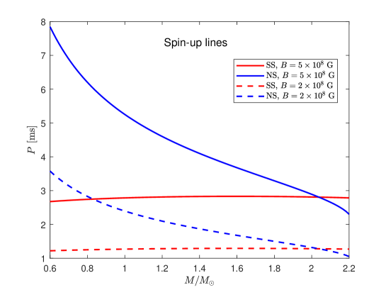
The spin-up condition written in equation (1) is an equation connecting mass and radius, so it is EoS-dependent. Different EoS models will give different spin-up lines in diagram. and Fig.1 shows the results for NS and SS models. Fig.1 shows the spin-up lines for both SS (red lines) and NS (blue lines) models, and the solid and dashed lines correspond to G and , respectively. We can see that the spin-up lines of NSs are decreasing with the mass, and that of SSs are nearly independent of the mass. The spin-up line gives the lower limit for spin-period of recycled pulsars, so Fig.1 indicates that an SS could have smaller values of than an NS in the recycling process.
3 The minimal spin-period by accretion
By accreting the amount of mass , the spin angular momentum added to a pulsar is given by , where is a numerical factor depending on the flow pattern (Ghosh & Lamb, 1979a) and is a dimensionless torque which could be assumed to be (Tauris et al., 2012). Then the final spin-period of a recycled pulsar (from rest) from the initial mass to the final mass could be estimated by
| (2) |
where is the (final) moment of inertia. We have assumed above that all the orbital angular momentum of the accreted material is transferred to the spin angular momentum of the pulsar, so in equation (2) is the minimal value of the final spin-period. In the following the values of are derived when the spin angular momentum of the star is calculated to the first order of spin angular velocity (Gao et al., 2022), which means that is independent of , and this approximation is good when the ms.
Besides the dependence of , and , the minimal spin-period determined by equation (2) also depends on which introduces and as variables. To estimate the differences in the minimal spin-period of a recycled pulsar between different EoS models, we make the same assumptions as in Tauris et al. (2012) that, the magnetic field decays rapidly in the early phases of the accretion process and accreting pulsars accumulate the majority of mass while spinning near equilibrium. In addition, we take as in Sec.2, since the dependence on is relatively weak. Consequently, the variables in the right-hand side of equation (2) are , , , and . Given an EoS, the minimal spin-period of a recycled pulsar with the amount of accreted mass could be derived.
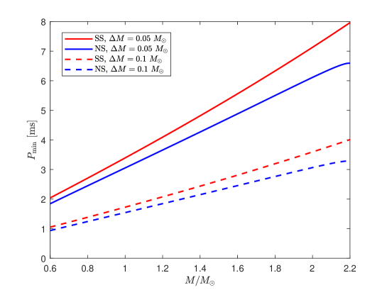
The and (final mass) relation for SS and NS models are shown in Fig.2, denoted respectively by red lines and blue lines, where solid lines represent the case of and dashed lines represent the case of . We can see that, with the same amount of accreted mass, NSs would spin faster than SSs. This is understandable: the radius of an NS is usually larger than that of an SS with the same mass, so an NS usually has larger than an SSs, which means that an NS could gain more angular momentum than an SS when the accreted mass is the same. In Fig.2 we choose G, and smaller values of will lift the lines upwards, since smaller will lead to smaller angular momentum transfer.
4 Comparison with observations
The recycling of pulsars is usual studied by comparison with observations in diagram. As we mentioned above, we keep as a parameter instead of replacing it by combination of and . Therefore, as shown in equations (1) and (2), in this paper the quantities to be compared with observations are and . Because equation (2) gives the minimal value of the final spin-period for a given value of , for a pulsar with a known value of it gives the minimum accreted mass . In the diagram, where denotes the final mass after accretion, we can plot the contours of for a given EoS by combining equations (1) and (2).
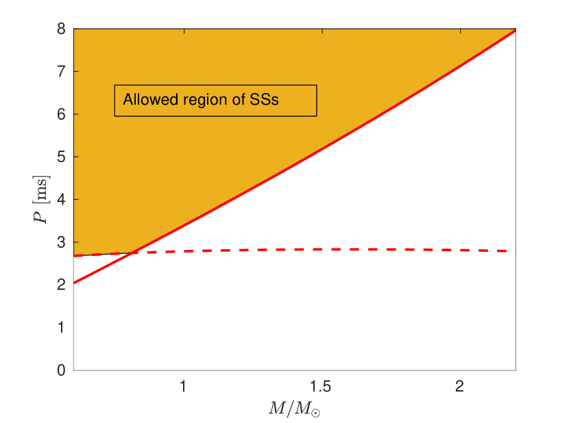
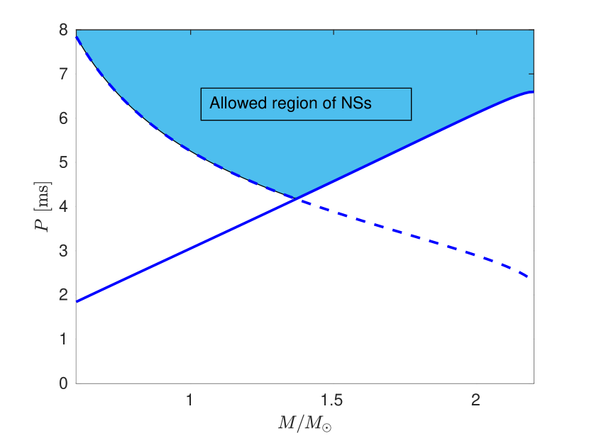
In the diagram, a higher contour of corresponds to a higher value of , and a lower curve of corresponds to a higher value of . Therefore, if we could determine the lower limit for and upper limit for , i.e. and , then the allowed region in diagram is above both the curves of and . Fig.3 shows the allowed regions of SSs (left) and NSs (right), where we adopt for solid curves and G for dashed curves. From this example we can see that, the allowed region of SSs covers the lower left region in diagram where NSs cannot reach, indicating that it could be easier for an SS to be fully recycled than that for an NS with the same when the mass is below about .
As mentioned above, to set the allowed region in diagram we should know the the lower limit for the magnetic field strength and the upper limit for the amount of accreted mass , although there are a lot of uncertainties to constrain and . We could estimate by considering that, the vacuum magnetic dipole model with inclination angle gives , so by setting we can get . It is interesting to noted that, for each pulsar whose data of and is plotted in Fig.4 (see below), the value of calculated using the data of and from the ATNF Pulsar Catalogue 111https://www.atnf.csiro.au/research/pulsar/psrcat/ (Manchester et al., 2005) is larger than the value of of the nearest dashed curve below it in diagram, under both SS and NS models. So setting as the lower limit of seems to be a reasonable way. It is also possible to estimate from the evolution process of the binary system, such as the accretion rate, the age of the MSP and the interaction between the MSP and the donor star.
To compare with observations, we extend the allowed regions shown in Fig.3 to different values of and , and we show in Fig.4 the results for SSs (left) and NSs (right). Solid curves correspond to , increasing downwards, and dashed curves correspond to contours for , increasing upwards. To ensure that the data are of fully recycled pulsars, we choose the masses of pulsars whose ms from Özel & Freire (2016) and plot their (with 1- uncertainties) and in this diagram.
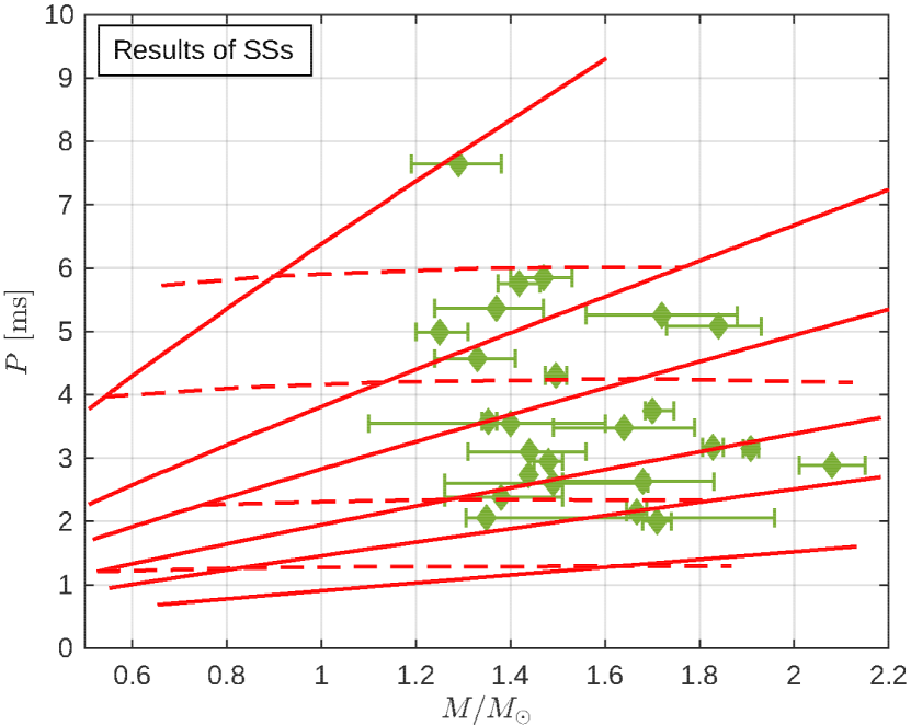
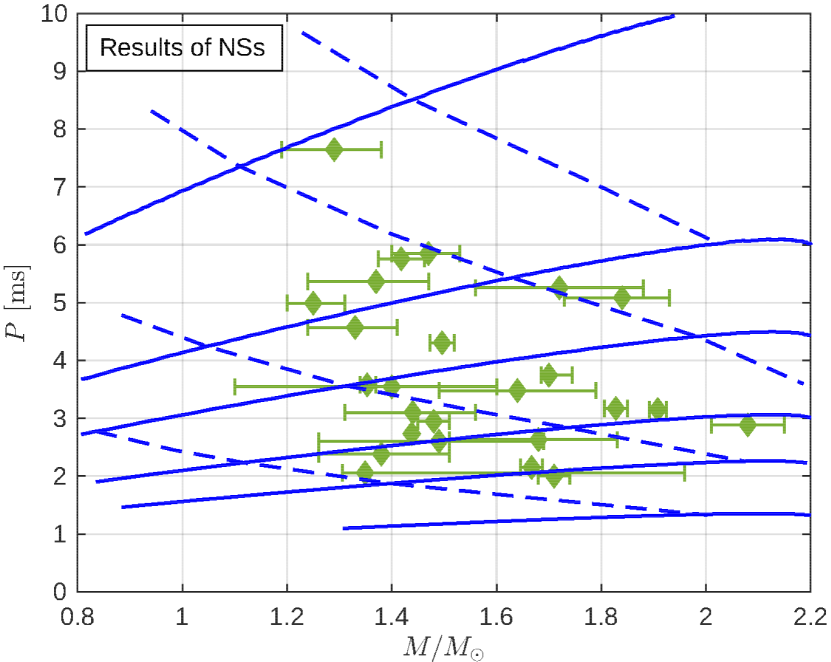
The different effects on parameters of recycled MSPs between SS and NS models can be seen from Fig.4. Although the curves of for SSs are not significantly different from that for NSs, the differences between the contours of for SSs and that for NSs are visible. The dashed curves in Fig. 4 show that the magnetic field strength will play an important role in impeding the spin-up of NSs, especially for the ones with low masses, but the impeding effect would not be important to SSs. The constraints on EoS models are more significant for masses below about than that for higher masses. For example, if the magnetic field is higher than G ( G), then an NS with () could not be spun up to ms ( ms), but an SS could. And on the other hand, if the magnetic field is higher than G, then an SS with mass approaching could not be spun up to ms, but an NS could.
As more and more masses of MSPs with increasing accuracy have been being measured, we can study the recycling of pulsars by comparison with observations in diagram. Although from the data plotted in Fig. 4 we could not yet disfavor neither SS nor NS models, finding more MSPs with ms with neither low mass or high mass in the future could help to put more strict constraints on the EoS of pulsars.
5 Conclusions and discussions
The global properties of pulsars determined by the EoS, such as mass, radius and the moment of inertia, could play a role in the spin-up process of accreting pulsars in binaries. We investigate the spin-up of MSPs in AP4 EoS of NS model and LX3630 EoS of the SS model. Combining the spin-up condition and the transferred angular momentum, we can constrain the accreted mass and the magnetic field strength of recycled MSPs. The allowed regions in diagram derived by the lower limit for and the upper limit for indicate that, it could be easier for an SS to form a low-mass and fully recycled MSP than that for an NS. Although the we could not yet rule out neither SS nor NS models by the present data, finding more samples of fully recycled MSPs with neither low mass (below about ) or very high mass (above about ) in the future could be helpful.
Although there are a lot of work about the recycling of MSPs which mainly focus on the effects of the interactions between pulsars and donor stars during binary evolution, the mass and radius are usually fixed to be typical values, such as and 10 km. We show in this paper, however, that different global structures could bring observational differences, implying that the effects brought by EoS models should be taken into account in studying the recycling of MSPs. It is worth adding the role of EoS to other effects, such as the nature of the donor star relating to the amount of accreted mass and evolution of the magnetic field due to accretion, to study the recycling of MSPs more comprehensively.
The AP4 EoS and the LX3630 EoS respectively represent EoS models of gravity-bound and self-bound, so we take them as examples to derive some universal conclusions. A gravity-bound pulsar, as shown by AP4 EoS, would have nearly unchanged radius when the mass increases from 1 to 2 , whereas the mass of a self-bound pulsar, as shown by LX3630 EoS, is nearly proportional to the third power of radius when the mass is well below the maximum value. This difference leads to different evolutions of during mass accretion, resulting in different allowed regions in diagram of recycled pulsars. We could make a general conclusion that, it is easier for a self-bound star to form a low-mass and fully recycled MSP than that for a gravity bound star. Finding more MSPs with spin periods less than 10 milliseconds and with accurate mass-measurement in the future, e.g. by SKA and FAST, could help to put more strict constraints on the nature of pulsars.
References
- Abbott et al. (2017) Abbott, B. P., et al. 2017, Phys. Rev. Lett., 119, 161101
- Akmal & Pandharipande (1997) Akmal, A., & Pandharipande, V. R. 1997, Phys. Rev. C, 56, 2261
- Alcock et al. (1986) Alcock, C., Farhi, E., & Olinto, A. 1986, ApJ, 310, 261
- Alford et al. (2008) Alford, M. G., Schmitt, A., Rajagopal, K., & Schäfer, T. 2008, Reviews of Modern Physics, 80, 1455
- Annala et al. (2018) Annala, E., Gorda, T., Kurkela, A., & Vuorinen, A. 2018, Phys. Rev. Lett., 120, 172703
- Bodmer (1971) Bodmer, A. R. 1971, Physical Review D, 4, 1601
- Bozzo et al. (2009) Bozzo, E., Stella, L., Vietri, M., & Ghosh, P. 2009, A&A, 493, 809
- Burderi & King (1998) Burderi, L., & King, A. R. 1998, ApJ, 505, L135
- Chen et al. (2021) Chen, H.-L., Tauris, T. M., Han, Z.-W., & Chen, X.-F. 2021, MNRAS, 503, 3540
- Cheng & Zhang (1998) Cheng, K. S., & Zhang, C. M. 1998, A&A, 337, 441
- Demorest et al. (2010) Demorest, P., Pennucci, T., Ransom, S., Roberts, M., & Hessels, J. 2010, Nature, 467, 1081
- Ertan & Alpar (2021) Ertan, Ü., & Alpar, M. A. 2021, MNRAS, 505, L112
- Gao et al. (2022) Gao, Y., Lai, X.-Y., Shao, L., & Xu, R.-X. 2022, MNRAS, 509, 2758
- Ghosh & Lamb (1979a) Ghosh, P., & Lamb, F. K. 1979a, ApJ, 234, 296
- Ghosh & Lamb (1979b) —. 1979b, ApJ, 232, 259
- Lai et al. (2023) Lai, X., Xia, C., & Xu, R. 2023, Advances in Physics X, 8, 2137433
- Lai & Xu (2009) Lai, X.-Y., & Xu, R.-X. 2009, Mon. Not. Roy. Astron. Soc., 398, L31
- Landau (1932) Landau, L. D. 1932, Phys. Z. Sowjetunion, 1, 285
- Lattimer & Prakash (2007) Lattimer, J. M., & Prakash, M. 2007, Phys. Rep., 442, 109
- Li et al. (2014) Li, L., Tong, H., Yan, W. M., et al. 2014, ApJ, 788, 16
- Manchester et al. (2005) Manchester, R. N., Hobbs, G. B., Teoh, A., & Hobbs, M. 2005, AJ, 129, 1993
- Özel & Freire (2016) Özel, F., & Freire, P. 2016, ARA&A, 54, 401
- Özel et al. (2010) Özel, F., Psaltis, D., Ransom, S., Demorest, P., & Alford, M. 2010, ApJ, 724, L199
- Podsiadlowski et al. (2002) Podsiadlowski, P., Rappaport, S., & Pfahl, E. D. 2002, ApJ, 565, 1107
- Spitkovsky (2006) Spitkovsky, A. 2006, ApJ, 648, L51
- Tauris et al. (2011) Tauris, T. M., Langer, N., & Kramer, M. 2011, MNRAS, 416, 2130
- Tauris et al. (2012) —. 2012, MNRAS, 425, 1601
- Tauris et al. (2000) Tauris, T. M., van den Heuvel, E. P. J., & Savonije, G. J. 2000, ApJ, 530, L93
- Tong (2016) Tong, H. 2016, Science China Physics, Mechanics, and Astronomy, 59, 5752
- Wang et al. (2011) Wang, J., Zhang, C. M., Zhao, Y. H., et al. 2011, A&A, 526, A88
- Weber (2005) Weber, F. 2005, Progress in Particle and Nuclear Physics, 54, 193
- Witten (1984) Witten, E. 1984, Phys. Rev. D, 30, 272
- Xu (2003) Xu, R.-X. 2003, Astrophys. J. Lett., 596, L59
- Zhang et al. (2023) Zhang, C., Gao, Y., Xia, C.-J., & Xu, R.-X. 2023, Phys. Rev. D, 108, 123031
- Zhang & Kojima (2006) Zhang, C. M., & Kojima, Y. 2006, MNRAS, 366, 137