RLER-TTE: An Efficient and Effective Framework for En Route Travel Time Estimation with Reinforcement Learning

Abstract.

En Route Travel Time Estimation (ER-TTE) aims to learn driving patterns from traveled routes to achieve rapid and accurate real-time predictions. However, existing methods ignore the complexity and dynamism of real-world traffic systems, resulting in significant gaps in efficiency and accuracy in real-time scenarios. Addressing this issue is a critical yet challenging task. This paper proposes a novel framework that redefines the implementation path of ER-TTE to achieve highly efficient and effective predictions. Firstly, we introduce a novel pipeline consisting of a Decision Maker and a Predictor to rectify the inefficient prediction strategies of current methods. The Decision Maker performs efficient real-time decisions to determine whether the high-complexity prediction model in the Predictor needs to be invoked, and the Predictor recalculates the travel time or infers from historical prediction results based on these decisions. Next, to tackle the dynamic and uncertain real-time scenarios, we model the online decision-making problem as a Markov decision process and design an intelligent agent based on reinforcement learning for autonomous decision-making. Moreover, to fully exploit the spatio-temporal correlation between online data and offline data, we meticulously design feature representation and encoding techniques based on the attention mechanism. Finally, to improve the flawed training and evaluation strategies of existing methods, we propose an end-to-end training and evaluation approach, incorporating curriculum learning strategies to manage spatio-temporal data for more advanced training algorithms. Extensive evaluations on three real-world datasets confirm that our method significantly outperforms state-of-the-art solutions in both accuracy and efficiency.

1. Introduction

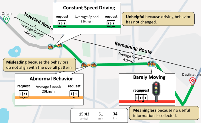
Figure 1. Real-time Requests in En Route Travel Time Estimation when Re-prediction is Ineffective

Travel Time Estimation (TTE) is one of the most critical operators in intelligent transportation systems, serving as the foundation for tasks such as route planning, vehicle dispatching, and navigation. Traditional TTE methods (Wang et al., 2018b, a; Fang et al., 2020; Yuan et al., 2020, 2022) provide a one-time estimation of travel time before the journey begins, lacking the capability for meaningful real-time updates during the trip. To address this limitation, the task of En Route Travel Time Estimation (ER-TTE) (Fang et al., 2021; Fan et al., 2022) has been developed, leveraging online data, such as the observed driving behavior of drivers, to enable more accurate online predictions.

Existing ER-TTE methods (Fang et al., 2021; Fan et al., 2022) primarily employ meta-learning techniques to quickly adapt to the unique characteristics of each individual trajectory. In online scenarios, users periodically initiate prediction requests during a journey. These methods receive the requests and utilize deep learning models to recalculate and provide more precise predictions. However, they overlook the complexity and dynamic nature of real-world traffic conditions, leaving critical gaps unaddressed.

(1) Inefficient prediction strategy. In real-world traffic scenarios, the variability of traffic conditions can lead to the collection of unhelpful and even misleading driving behavior data. As shown in Figure 1, we illustrate three situations where the newly collected data between two consecutive requests is ineffective for travel time estimation. First, when the vehicle is traveling at a constant speed, the newly collected driving behavior remains consistent with the previously learned behavior, offering no additional benefit. Second, there may be a unique road segment that deviates from the general driving pattern before and after, potentially introducing noise and misleading the prediction. Lastly, when the vehicle has barely moved between two requests, no meaningful new data is collected, rendering the data meaningless for further prediction. Additionally, TTE servers in real-world applications handle billions of real-time requests daily. However, existing methods handle these requests by entirely relying on computationally intensive deep learning models for re-calculation. This strategy not only yields minimal improvements in prediction accuracy in many cases but also imposes significant computational stress on the TTE servers. Therefore, it is crucial to develop an innovative solution that can provide accurate real-time predictions while ensuring high efficiency.

(2) Dynamic scenarios and complex data correlations. To formulate wise prediction strategies, a significant challenge lies in evaluating the quality of online data. Although some simple scenarios are described in Fig. 1, we contend that real-world situations are far more complex. Traffic environments are characterized by dynamic changes and uncertainties, making it difficult to define these problems with explicit rules or models. Moreover, there are intricate spatio-temporal correlations between online data and offline data (e.g., road networks and trajectories). Different road segments exhibit heterogeneous attributes, such as varying speed limits, which correspond to different driving behaviors. However, existing methods for handling these two types of data merely perform simple concatenation, lacking specialized designs to effectively capture the complex correlations between the data. We argue that an ideal solution should thoroughly explore the relationships between the two data types and be capable of making accurate autonomous decisions.

(3) Flawed training and evaluation. Despite claims of outstanding performance by existing ER-TTE methods, their training and evaluation approaches have certain flaws that fail to reveal their true capabilities in online scenarios. Traditional TTE training methods (Wang et al., 2018b; He et al., 2019; Fang et al., 2020) treat an entire trajectory as a single training sample because they only make one prediction at the beginning of the journey. However, in ER-TTE, each trajectory corresponds to numerous prediction requests along the way, with each request having different traveled and remaining routes. Thus, a single trajectory actually corresponds to multiple training samples. Existing methods (Fan et al., 2022; Fang et al., 2021) generate datasets with a fixed proportion of traveled journeys for both training and evaluation. For instance, using a fixed proportion such as 30% of the traveled route for all trajectories means that each trajectory corresponds to only one prediction request, thus serving as a single training sample. This training strategy results in models that perform poorly when handling prediction requests with different proportions of traveled routes, thereby failing to effectively address all requests for the entire trajectory. Therefore, it is crucial to establish an effective training strategy.

To address the aforementioned challenges, we present a novel framework, RLER-TTE, designed for efficient and robust en route travel time estimation. To address the first challenge, we propose a novel pipeline that redefines the data flow in an online data processing system for ER-TTE. The framework resolves the tradeoff between reusing results and invoking effective models when handling large-scale ER-TTE requests. In online prediction scenarios, the system continuously receives newly collected online data along with prediction requests. Instead of recalculating all requests, the requests first pass through a lightweight Decision Maker, which analyzes the driving patterns from the complex online data and determines whether the newly collected information can improve the predictions. Following this decision, a Predictor will decide whether to invoke the computationally intensive prediction model or to infer directly from historical prediction results, based on the decision outcomes. Next, in response to the second challenge, we model the online decision-making problem as a Markov Decision Process and carefully design states that effectively represent the complex dynamics of online traffic scenarios, along with a well-defined reward function. We refine the definition of the state to ensure it captures the intricate correlations between online and offline data. Reinforcement learning, specifically Q-learning, with meticulously designed feature encoding techniques and an efficient model architecture, is employed to enable online decision-making. We demonstrate how machine learning techniques can be innovatively applied to online data processing systems, and our strategies can be broadly extended to other similar real-time decision-making systems. Finally, to address the third challenge, we introduce a curriculum learning strategy and propose an end-to-end training and evaluation method. For each trajectory, we assume that users initiate requests at fixed time intervals, resulting in multiple training samples with varying proportions of traveled segments. This approach generates a large volume of training data. Training in a randomly shuffled order significantly reduces efficiency and slows down convergence. To mitigate this, we design a curriculum by assessing the difficulty of all training samples and selectively arranging the learning sequence. Since the difficulty of samples from trajectories of different lengths cannot be directly compared, we first partition the data into non-overlapping metasets and evaluate them within each metaset. Subsequently, we propose a training scheduling algorithm that arranges the curriculum based on the assessed difficulty.

In summary, the main contributions are listed as follows.

• We introduce a novel framework, RLER-TTE, which for the first time establishes an en route travel time estimation pipeline consisting of two primary components: the Decision Maker and the Predictor. This framework redefines the data flow of online data processing in the ER-TTE system, significantly enhancing overall system efficiency and performance (Sec. 3).

• We define a Markov decision process to address decision-making challenges in complex real-time scenarios and carefully design the state and reward functions to ensure the effective operation of the system. Additionally, we employ reinforcement learning techniques as a decision-making tool and design feature representation and encoding methods. Our work demonstrates the practical application of ML techniques in solving data management challenges. (Sec. 4)

• We propose an end-to-end training method for the Predictor and define a more scientific evaluation methodology, establishing new standards for the ER-TTE system. In addition, we introduce a curriculum learning strategy to manage trajectory data, incorporating two carefully designed components: the Trajectory Difficulty Measurer and the Training Scheduler. These components accelerate model convergence and guide the model towards better minima in the parameter space (Sec. 5).

• We conduct a comprehensive evaluation on three real-world datasets and demonstrate that our approach significantly outperforms existing methods in terms of both accuracy and efficiency. (Sec. 6)

2. PRELIMINARIES

We first introduce some basic concepts and then formalize the problem of ER-TTE.

2.1. Basic Concepts

Road Network. The road network can be formally represented as a directed graph $G=\langle V,E\rangle$, where $V$ denotes the set of vertices corresponding to the endpoints of road segments, and $E$ represents the set of directed edges, each corresponding to a road segment connecting a pair of vertices in $V$.

Travel Route. A raw trajectory consists of a sequence of GPS points, each denoted as $\langle[\phi_{i},\psi_{i}],t_{i}\rangle$. Here, $\phi_{i}$ and $\psi_{i}$ represent the spatial coordinates—latitude and longitude, respectively, and the term $t_{i}$ designates the timestamp. We utilize existing map-matching algorithms (Brakatsoulas et al., 2005; Wenk et al., 2006) that have been broadly adopted in the field (Yuan and Li, 2019; Wang et al., 2022a) to associate these GPS points with specific road segments. Simultaneously, we calculate the travel time for each road segment as $y_{i}=t_{i}[-1]-t_{i}[1]$, where $t_{i}[1]$ and $t_{i}[-1]$ denote the start and end timestamp, respectively. Notably, we employ the linear interpolation technique to compute $t_{i}$. Consequently, a travel route $\mathcal{R}$ can be represented as a sequence of connected links $\{l_{1},l_{2},\ldots,l_{m}\}$, where $l_{i}=\langle e_{i},y_{i}\rangle$ and $e_{i}$ is the $i$-th road segment.

2.2. Problem Definition

Travel Time Estimation. We define a Travel Time Estimation (TTE) request as $req=(\mathcal{R},\rho)$, where $\mathcal{R}$ denotes the travel route and $\rho$ represents the departure time of the route. The objective of TTE is to predict the total travel time for the entire travel route based on the issued request $req$.

En Route Travel Time Estimation. The ER-TTE task is aimed at real-time prediction in online scenarios. As users drive en route, the ER-TTE system continuously receives prediction requests. To clarify, we represent the sequence of requests in chronological order as $[t_{1},t_{2},...,t_{n}]$, where $n$ denotes the number of requests. Assuming a request is issued at time $t$, the request can then be formalized as $req=(\mathcal{R},\rho,t)$, where the route $\mathcal{R}$ can be divided into two parts: the segments already traveled, denoted as $\mathcal{R}_{traveled}=\{l_{1},l_{2},\ldots,l_{i^{t}-1}\}$, and the segments yet to be traveled, denoted as $\mathcal{R}_{remain}=\{l_{i^{t}},l_{i^{t}+1},\ldots,l_{m}\}$. The actual travel times of the traveled route segments, denoted as $Y_{traveled}=\{y_{1},y_{2},\ldots,y_{i^{t}-1}\}$, are considered as online information reflecting the user’s past driving behavior. Conversely, the time associated with the remaining route, denoted by $Y_{remain}=\{y_{i^{t}},y_{i^{t}+1},\ldots,y_{m}\}$, serves as the output of the ER-TTE task.

3. Framework Overview

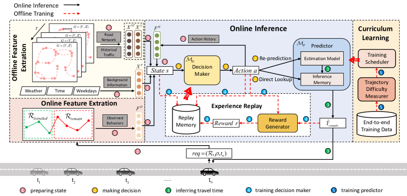
Figure 2. Architecture of the RLER-TTE Framework

In this section, we provide a comprehensive description of our system, RLER-TTE. Unlike existing systems that re-predict travel time for each real-time request, our approach incorporates an action selection mechanism to determine whether previous prediction results can be reused. To achieve this, we integrate a reinforcement learning pipeline into the online inference process. As illustrated in Figure 2, our system comprises five modules. The Offline Feature Extraction and Online Feature Extraction modules are designed to extract relevant features. The Online Inference module consists of two deep learning components: Decision Maker $\mathcal{M}_{D}$ and Predictor $\mathcal{M}_{P}$. Here, $\mathcal{M}_{D}$ decides whether to re-predict new results with $\mathcal{M}_{P}$ or use historical prediction results. Finally, Curriculum Learning and Experience Replay modules are proposed to offline train $\mathcal{M}_{P}$ and $\mathcal{M}_{D}$. Next, we elaborate on the whole pipeline within our system, detailing the interactions among the five modules.

Preparing state. Suppose at time $t_{n}$, the user has a request $req=(\mathcal{R},\rho,t_{n})$. The Offline Feature Extraction module extracts pre-computed spatio-temporal information of the route, which are commonly utilized features in the TTE task (Fang et al., 2020; He et al., 2019; Yuan et al., 2022). These include spatial-only features ($X^{S}$), temporal-only features ($X^{T}$), and spatio-temporal features ($X^{ST}$). Specifically, the spatial-only features ($X^{S}$) are derived from the road network and represent the attributes of road segments (e.g., ID, length, speed limit), as well as their geographical relations. For a given route $\mathcal{R}$, we define $X^{S}=\{x^{s}_{l_{i}}\}_{l_{i}\in\mathcal{R}}$, where $x^{s}$ denotes the spatial attributes of road segment $l_{i}$. The temporal-only features ($X^{T}$) consist of attributes from the past $p$ time slots, including departure time, weekdays, and weather conditions. For each segment at the current time $t_{c}$, we define $X^{T}=\{\{x^{t}\}^{j}_{l_{i}}\}^{j\in[t_{c}-p:t_{c}]}_{l_{i}\in\mathcal{R}}$. Similarly, the minimum, maximum, median, and average values of traffic speeds for road segments over the past $p$ time periods are calculated as historical traffic conditions, which encompass the spatio-temporal features ($X^{ST}$). These features are defined as $X^{ST}=\{\{x^{st}\}^{j}_{l_{i}}\}^{j\in[t_{c}-p:t_{c}]}_{l_{i}\in\mathcal{R}}$, where $x^{st}=\{v_{min},v_{max},v_{med},v_{avg}\}$.

Simultaneously, the Online Feature Extraction module extracts real-time driving behaviors ($F^{D}$) from the traveled route. $F^{D}$ are primarily obtained from the actual speed over the traveled road segments, reflecting the user’s driving patterns, and is defined as $F^{D}=\{f^{d}_{l_{i}}\}_{l_{i}\in\mathcal{R}_{traveled}}$. Additionally, we maintain a record, denoted as $F^{H}$, of the decision history provided by the Decision Maker, which is defined as $F^{H}=\{f^{h}_{l_{i}}\}_{l_{i}\in\mathcal{R}_{traveled}}$. Collectively, these online features and offline features constitute the state $s$.

Making decision. After feature extraction, the state $s$, which comprehensively represents the entire route and indicates the current position, is passed to the agent Decision Maker $\mathcal{M}_{D}$. This agent utilizes a model to generate the action within the reinforcement learning pipeline. Specifically, we employ the Double Deep Q-Network (Double DQN) (van Hasselt et al., 2016) as the learning algorithm, which significantly reduces the overestimation of action values and enhances the stability of the learning process in dynamic environments. The network evaluates potential actions and selects the one with the highest value. For actions, we have designed two options: one is to invoke a more complex deep learning model in the Predictor for re-prediction, and the other is to directly look up the Inference Memory in the Predictor, which continuously stores the most recent prediction results.

Inferring travel time. The Predictor $\mathcal{M}_{P}$ comprises the Estimation Model and the Inference Memory, which receives and executes the action $a$. The Estimation Model, a sophisticated neural network designed to calculate travel time, employs two state-of-the-art ER-TTE methods, SSML (Fang et al., 2021) and MetaER-TTE (Fan et al., 2022), to validate the robustness of our approach. Each time a new calculation is performed, the prediction results are stored in the Inference Memory, which can quickly provide prediction results for subsequent requests. The final result, $\hat{Y}_{remain}$, representing the estimated time for the remaining route, is then conveyed to the user terminal.

Training decision maker. During the training phase, the models within the Decision Maker and Predictor modules are trained independently. For the Decision Maker module, we utilize the widely adopted Experience Replay mechanism in reinforcement learning, where an experience is represented as a tuple consisting of state, action, reward, and next state. The processes for generating the state and action have been previously detailed. The reward is derived from the Reward Generator, which considers the estimated results $\hat{Y}_{remain}$ and the decision action $a$, comprehensively evaluating efficiency and performance to compute the reward associated with the action. This tuple is then stored in the Replay Memory, which maintains a fixed-size buffer.

Training predictor. In our end-to-end model training method, each trajectory encompasses numerous request instances, resulting in a substantial increase in the quantity of training data and considerable variation in quality. To address this, we introduce a curriculum learning strategy to enhance the training of TTE models within the Predictor. Specifically, we employ a Trajectory Difficulty Measurer to assess the complexity of predicting a trajectory based on multiple metrics. Subsequently, the Training Scheduler devises a curriculum for the Predictor to follow.

4. Online Decision-Making

In this section, we provide a detailed description of our online decision-making mechanism based on reinforcement learning. Firstly, we discuss how to formulate this problem as a Markov Decision Process (MDP) in Sec 4.1. Secondly, we explain the model architecture in Sec 4.2, which is specifically engineered to facilitate efficient decision-making within online environments. Lastly, in Sec 4.3, we elaborate on the training algorithm employed to optimize the model’s performance, accompanied by a complexity analysis.

4.1. MDP Formulation

State. At step $t$, the corresponding state $s_{t}$ comprises two types of features: offline features and online features. Offline features ($X^{S},X^{T},X^{ST}$), which can be obtained prior to the start of the journey, reflect the static characteristics of the route. In contrast, online features ($F^{D},F^{H}$) are acquired in real-time during the journey. These are utilized to assess the value, neutrality, or potential misleading nature of newly collected online information from the last prediction made by the Predictor to the current prediction request. For the Decision Maker, online features are crucial for making accurate decisions. Specifically, driving behavior ($F^{D}$) and decision history ($F^{H}$) are pivotal because they collectively capture the driver’s unique driving pattern. By incorporating offline features, the Decision Maker can further analyze the relationship between these patterns and static route characteristics, thereby enabling more informed decision-making. In contrast, the Predictor focuses on leveraging offline features to make accurate travel time predictions. Particularly, the segment length from $X^{S}$ and the traffic conditions provided by $X^{ST}$ form the foundational basis of prediction, while other features further refine the prediction details.

Action. We define two types of actions: (1) recalculate the travel time for the current request using the Estimation Model in Predictor; (2) directly provide the estimated value from the Inference Memory. For the sake of clarity, these two actions are referred to as “re-prediction” and “direct lookup” hereafter.

Transition. In the ER-TTE process, given a state $s_{t}$ and a corresponding action $a_{t}$, the transition will move to the state $s_{t+1}$, which incorporates the newly acquired information of the traveled segment along the route. In particular, the online features $F^{D}$ and $F^{H}$ would be updated within the new state.

Reward. The design of the reward function is crucial in reinforcement learning as it significantly impacts the method’s effectiveness. To achieve outstanding performance and efficiency, our reward design must comprehensively consider both aspects. Therefore, our reward function is composed of three components: performance, efficiency, and frequency.

The performance reward directly reflects the accuracy of the travel time prediction results. A straightforward idea is to use the prediction result itself as the reward. However, the range of prediction values can vary significantly across different predictions, making it difficult for Decision Maker to evaluate the quality of actions effectively. To address this issue, a reward function capable of eliminating the base value of the predictions and amplifying the differential can be introduced to ensure that the reward is consistent and comparable across different predictions. To formalize this, we need to calculate Predictor’s prediction value as the re-prediction result, denoted as $\hat{y}_{rp}$. Simultaneously, we define $\hat{y}_{dl}$ as the direct lookup result. The difference between these two predictions is used as the reward, which is defined as follows:

(1) $$r_{p}=\begin{cases}-(\hat{y}_{dl}-\hat{y}_{rp})&a_{i}=0\\ -(\hat{y}_{rp}-\hat{y}_{dl})&a_{i}=1\end{cases}$$

where $a_{i}=0$ denotes direct lookup and $a_{i}=1$ denotes re-prediction.

The efficiency reward imposes a certain penalty each time the Predictor is used to encourage efficient usage. By setting a penalty factor $\omega_{p}$, it ensures that when the improvement achieved through re-prediction is limited, the framework can choose to directly provide the prediction result instead. By adjusting the value of the penalty factor, we can trade-off between performance and efficiency. The efficiency reward is defined as follows:

(2) $$r_{e}=\begin{cases}0&a_{i}=0\\ \omega_{p}&a_{i}=1\end{cases}$$

The frequency reward limits the usage frequency of the Predictor to a certain extent, balancing efficiency and performance. This reward mechanism is designed to influence the Decision Maker’s behavior, encouraging it to make direct lookup soon after utilizing the Predictor and to favor re-prediction after a long period without using the Predictor. To achieve this, the reward is formulated based on the elapsed time between the last prediction made by the Predictor and the current request. Our goal is to ensure that the framework remains dataset-agnostic and is not tied to a specific Predictor. Therefore, we implemented a linear function to model this reward, which ensures robustness due to its simplicity and stable growth pattern.

(3) $$r_{f}(\sigma)=\begin{cases}0&a_{i}=0\\ \alpha\cdot\sigma+\beta&a_{i}=1\end{cases}$$

Where $\alpha$ and $\beta$ are hyper-parameters, $\sigma$ represents the time interval between the last prediction and the current time. The value of the linear function transitions from negative to positive as $\sigma$ increases.

Finally, we can evaluate the overall reward as follows:

(4) $$r=r_{p}+r_{e}+r_{f}(\sigma)$$

4.2. Model Architecture

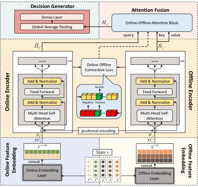
Figure 3. The Architecture of Decision Maker

In Section 3, we provide an overview of the Decision Maker, designed to generate decisions efficiently from both online and offline features. As shown in Fig. 3, we will elaborate on its components, offering a more granular understanding of their structures and functions.

Feature Embedding. Each road segment is characterized by a series of attributes, including its id, length, and other relevant features. The embedding layer is designed to encode these discrete attribute values into dense vectors. We employ established and widely-used graph embedding techniques (Grover and Leskovec, 2016) to model the road network’s graph structure. The embedding vector for a road segment is denoted as $h_{s}\in\mathbb{R}^{d_{s}}$. Assuming the size of the time slot is defined as $\Delta T$ minutes, we segment them into weekly cycles, obtaining their embeddings $h_{t}\in\mathbb{R}^{\frac{7\times 24\times 60}{\Delta T}}$. For the traffic conditions, we first embed the data according to the time slots. Subsequently, we incorporate the historical time slots to obtain the final embedding representation, denoted as $h_{st}\in\mathbb{R}^{T\times d_{st}}$, where $T$ is the number of historical time slots. Finally, we concatenate these embeddings and pass them through a fully connected layer ($FC_{1}$) with ReLU as the activation function to obtain the dense vector of offline features: $H_{X}=Dense(concat(h_{s},h_{t},h_{st}))$.

The embeddings of driving behaviors and decision history are denoted by $h_{d}$ and $h_{h}$. Through another fully connected layer ($FC_{2}$), we embed them into $H_{F}$, which is formulated as $H_{F}=Dense(concat(h_{d},h_{h}))$.

Offline Encoder & Online Encoder. To efficiently capture the internal correlations of both online and offline features, we design two modules to encode them separately. These two modules share a similar structure of attention blocks, as the attention mechanism is more efficient in handling sequential data and has demonstrated exceptional performance in capturing the spatio-temporal correlations (Luo et al., 2021; Tan et al., 2023). For the sake of clarity, we will illustrate the architecture using the offline feature encoder as an example. Specifically, each block comprises the following components:

Multi-Head Self-Attention: The encoder leverages the Multi-Head Self-Attention mechanism to capture intricate dependencies within the input features $H_{X}$. Firstly, we define the query ($Q_{c}=\mathbf{W}_{q}H_{X}$), the key ($K_{c}=\mathbf{W}_{k}H_{X}$), and the value ($V_{c}=\mathbf{W}_{v}H_{X}$), where $\mathbf{W}_{q}$, $\mathbf{W}_{k}$, and $\mathbf{W}_{v}$ are learnable parameters. The self-attention score is computed by $score(H_{X},H_{X})=softmax\left(\frac{Q_{c}\cdot(K_{c})^{\top}}{\sqrt{d_{m}}}\right)$, where $d_{m}$ denotes the size of vector $Q_{c}$. Subsequently, we obtain the new encoded representation $Z_{c}=score(H_{X},H_{X})\cdot V_{c}$. This mechanism allows the model to attend to different parts of the input sequence simultaneously, thereby enhancing the representation capability.

Add & Normalize: This layer comprises two key operations: residual connection and layer normalization. The residual connection is employed to mitigate the vanishing gradient problem, while layer normalization standardizes the inputs to have zero mean and unit variance. The process can be represented as $H_{N}=LN(H_{X}\oplus Z_{c})$.

Feed Forward: To further transforming the encoded representations, we design a fully connected layer, which can be expressed as $Z_{f}=ReLU(\mathbf{W}_{f}H_{N}+b_{f})$, where $\mathbf{W}_{f}$, and $b_{f}$ are learnable parameters and $ReLU(\cdot)$ is the activation function.

Add & Normalize: Similar to the previous layers, we further enhance the encoding: $\hat{H}_{c}=LN(H_{N}\oplus Z_{f})$.

The aforementioned four steps constitute the fundamental block of the encoder. By employing these encoder blocks, we obtain representations for both online and offline features, denoted as $\overline{H}_{c}$ and $\hat{H}_{c}$, respectively.

Contrastive Learning. Contrastive learning aims to align online features and offline features, thereby enhancing the encoders’ capacity to learn superior feature representations. For a batch of training examples, feature pairs of the same sample are considered positive pairs, while pairs from different samples are negative pairs. We first project the online feature $\overline{H}_{C}$ and the offline feature $\hat{H}_{C}$ into a higher-dimensional space through linear transformations to obtain the normalized representations, denoted as $g_{n}(\overline{H}_{C})$ and $g_{f}(\hat{H}_{C})$. To quantify the similarity between the online and offline features, we define a similarity function $S_{ij}=g_{n}(\overline{H}_{C}^{(i)})^{\top}g_{f}(\hat{H}_{C}^{(j)})$, where $i$ and $j$ index the samples in the batch. The alignment between the online and offline features is reinforced using the InfoNCE loss, which aims to maximize the similarity scores between positive pairs. The InfoNCE loss $L_{c}$ is computed as follows:

(5) $$\mathcal{L}_{c}=-\frac{1}{N}\sum_{i=1}^{N}\log\frac{\exp(S_{ii}/\tau)}{\sum_{j=1}^{N}\exp(S_{ij}/\tau)}$$

where $N$ denotes the batch size, and $\tau$ represents the temperature parameter.

Online-Offline-Attention Fusion. To obtain a comprehensive representation of the current state, we apply an attention mechanism to further integrate the online and offline features. Specifically, the online feature $\overline{H}_{c}$ serves as the query, while the offline feature $\hat{H}_{c}$ is used as both the key and value. The fusion process is summarized by the following formula: $H_{c}=softmax\left(\frac{\overline{H}_{c}\cdot\hat{H}_{c}^{\top}}{\sqrt{d_{a}}}\right)\hat{H}_{c}$, where $d_{a}$ denotes the dimension of the feature space. Thus, the online feature $\overline{H}_{C}$ guides the integration of the offline feature $\hat{H}_{C}$, allowing the model to focus on the most relevant aspects of the offline information, effectively combining the feature representations into a coherent form.

Decision Generator. In the final step, we utilize Global Average Pooling followed by a Dense Layer to aggregate the feature representations and predict action values: $Q=Dense(Avg(h_{c}))$, where $Q$ represents the value associated with each possible action, and the action with the highest value is selected as the output.

Input : training inputs $\mathbf{Z}$, training labels $\mathbf{Y}$, the Decision Maker $\mathcal{M}_{dc}$, the Predictor $\mathcal{M}_{p}$, experience buffer $\mathcal{B}$, learning rate $lr$, training epochs $ep$, batch size $bs$, loss weight $\lambda$, discount factor $\gamma$, update step $us$, train step $ts$.

Output : parameters $\theta_{dc}$ for the Decision Maker $\mathcal{M}_{dc}$.

1

2$X,F\leftarrow$ generating online and offline features;

3 initialize $\theta_{dc}$ with normal distribution;

4 for $m\leftarrow 1\ldots ep$ do

5    $\theta_{dc}\leftarrow ModelTrain(\mathbf{Z},\mathbf{Y},\mathcal{B},X,F,lr,bs,\lambda,\gamma,ts)$;

6    update the main network with $\theta_{dc}$;

7    if $m\mod us=0$ then

8       update the target network;

9      

10   

Algorithm 1 Model Learning for RLER-TTE

Input : $\mathbf{Z},\mathbf{Y},\mathcal{B},X,F,lr,bs,\lambda,\gamma,ts$

1 iterations $I=|\mathbf{Z}|$;

2

3for $i\leftarrow 1\ldots I$ do

4    $s_{i}\leftarrow X_{i},F_{i}$;

5    $a_{i}\leftarrow(\mathcal{M}_{emb},\mathcal{M}_{enc},\mathcal{M}_{atf},\mathcal{M}_{dcg})(s_{i})$;

6    $\hat{Y}_{i}\leftarrow\mathcal{M}_{p}(X_{i}^{S},X_{i}^{T},X_{i}^{ST},F_{i}^{D})$;

7    $r_{i}\leftarrow$ using Equations 1-4 with $a_{i}$ and $\hat{Y}$;

8    $s_{i+1}\leftarrow X_{i+1},F_{i+1}$;

9    construct transition $T_{i}=\{s_{i},a_{i},r_{i},s_{i+1}\}$ and store into $\mathcal{B}$;

10    if $i\mod ts=0$ then

11       random sample transitions $T$ from $\mathcal{B}$ based on $bs$;

12       training iterations $TI=|T|$;

13       for $j\leftarrow 1\ldots TI$ do

14          compute $q,q_{target}$ with main and target network;

15          $\mathcal{L}\leftarrow$ using Equations 5, 6, 7 and $\lambda$;

16         

17      

18   

return $\theta_{dc}$;

Function 2 ModelTrain

4.3. Model Learning

As shown in Algorithm 1, we delineate the process of model learning for RLER-TTE. We first extract the offline features $X$ and online features $F$. We then initialize the parameters of all modules using a normal distribution.We train the model for the specified number of epochs $ep$. During each epoch, we execute the ModelTrain procedure to optimize the main network and periodically update the target network according to the update step $us$.

Model Train. In each iteration, we utilize $X_{i}$ and $F_{i}$ to construct the state $s_{i}$. Subsequently, the state $s_{i}$ is processed by the model architecture described in Section 4.2 to produce the action $a_{i}$. Concurrently, the Predictor module produces the new prediction $\hat{Y}_{i}$. The reward $r_{i}$ is computed based on $a_{i}$ and $\hat{Y}_{i}$, using Equations 1-4. Next, we construct a transition $T_{i}$ and store it in the experience buffer $\mathcal{B}$. Based on the train step $ts$, we train the model whenever a certain amount of new data is added to $\mathcal{B}$. Specifically, we employ a Temporal Difference (TD) learning strategy to train our double DQN network. First, we use the main network to compute the Q-values of the actions and select the action $a_{j+1}^{*}$ with the highest Q-value. Then, the target network evaluates the chosen action’s Q-value in the next state $s_{j+1}$. This Q-value, multiplied by the discount factor $\gamma$ and added to the current reward $r_{j}$, forms the target Q-value: $q_{\text{target}}=r_{j}+\gamma\cdot\max_{a^{\prime}}Q_{\text{target}}(s_{j+1},a^{\prime})$. The Huber Loss is used to compute the TD loss, which is formulated as:

(6) $$\mathcal{L}_{td}=\begin{cases}\frac{1}{2}(q-q_{\text{target}})^{2},&\text{if }|q-q_{\text{target}}|<\delta\\ \delta\cdot(|q-q_{\text{target}}|-\frac{1}{2}\delta),&\text{if }|q-q_{\text{target}}|>\delta\end{cases}$$

where $\delta$ is the scale parameter, $q$ represents the Q-value of the main network, and $q_{\text{target}}$ denotes the Q-value of the target network. Incorporating the contrastive loss $\mathcal{L}_{c}$, the overall learning objective is formulated as follows:

(7) $$\mathcal{L}=\mathcal{L}_{td}+\lambda\cdot\mathcal{L}_{c}$$

where $\lambda$ is the hyper-parameter that adjusts the weighting of the different loss functions.

Complexity Analysis. Our framework is designed to improve overall system efficiency by using a lightweight Decision Maker to reduce the frequency of Predictor invocations. Since the Decision Maker introduces additional overhead to achieve this improvement, its efficiency must significantly surpass that of the Predictor. Therefore, to verify this, we compare the computational complexity and number of parameters of the proposed reinforcement learning module with two ER-TTE methods SSML (Fang et al., 2021) and MetaER-TTE (Fan et al., 2022) and a TTE methods ConST (Fang et al., 2020). Specifically, we model the problem input as follows: the travel route comprises $n$ road segments, the batch size is $b$, and the historical time slots are defined as $T$. We assume that the dimensions of all hidden representations are $d$.

Both of the two ER-TTE methods are based on ConST, utilizing the same embedding technique and a 3D graph attention mechanism. The embedding layer has $O(Tnd)$ parameters, and the 3DGAT contains three dense layers, with a total parameter count of $O(d^{2})$. Following this, ConST employs a convolutional layer with a window size of $w$, having $O(wd^{2})$ parameters. The complexity of computing attention scores is $O(bn^{2}d)$, and the combined complexity of computing attention outputs is $O(bn^{2}d+bn^{2})$. Considering the complexity for each convolutional layer calculation over the entire window, it is $O((2w+1)\cdot d\cdot d)$, and taking into account batch size and sequence length, the overall complexity is $O(bnwd^{2})$. Overall, the computational complexity of ConST is $O(bnwd^{2}+bn^{2}d+bn^{2})$.

Table 1. Complexity Analysis of the Main Methods

	#Params	Complexity
ConST	$O(wd^{2})$	$O(bnwd^{2}+bn^{2}d+bn^{2})$
SSML	$O(d^{2})$	$O(bn^{3}d+bnd^{2}+bn^{2}d)$
MetaER-TTE	$O((K+w)d^{2})$	$O(bnwd^{2}+bn^{2}d+bd^{2}+bKd)$
Decison Maker	$O(d^{2})$	$O(bn^{2}d+bnd^{2})$

For SSML, it employs a model-based meta-learning approach. In the representation learning phase, the 3DGAT is computed for each sample in the query set and the validation set, with a complexity of $O(n^{2}d)$ and a parameter count of $O(d^{2})$. For all samples in the batch, this results in a complexity of $O(bn^{3}d)$. Subsequently, an MLP with complexity $O(bnd^{2})$ and an attention layer with complexity $O(bn^{2}d)$ are applied. Both of these layers have parameter counts of $O(d^{2})$, and the overall complexity of SSML is $O(bn^{3}d+bnd^{2}+bn^{2}d)$.

For MetaER-TTE, an optimization-based meta-learning approach is utilized. First, the trajectory query vectors are computed with a complexity of $O(bd^{2})$, followed by the calculation of similarity scores with a complexity of $O(bKd)$, where $K$ represents the number of cluster centers. Next, a Cluster-aware Parameter Memory is employed, with a parameter size of $O(Kd^{2})$ and a computational complexity of $O(d^{2}+Kd)$. Finally, it propose a learning rate generator, which is a multi-layer MLP with a parameter count of $O(d^{2})$ and a computational complexity of $O(bd^{2})$. Combined with the base model, the total computational complexity is $O(bnwd^{2}+bn^{2}d+bd^{2}+bKd)$.

As for RLER-TTE, the complexity is primarily dominated by the Encoder layer. The Encoder has a parameter count of $O(d^{2})$, and its computational complexity includes the attention mechanism with $O(bn^{2}d)$ and the fully connected layers with $O(bnd^{2})$. The subsequent modules also encompass these two components. Hence, the overall complexity is $O(bn^{2}d+bnd^{2})$.

Remark: The complexity of the reinforcement learning module in RLER-TTE is an order of magnitude lower than that of several baseline methods. Consequently, as demonstrated in our experiments, the efficiency of RLER-TTE relative to the Predictor closely matches the model usage rate, with the computational cost of reinforcement learning constituting only a small fraction.

5. Curriculum Learning

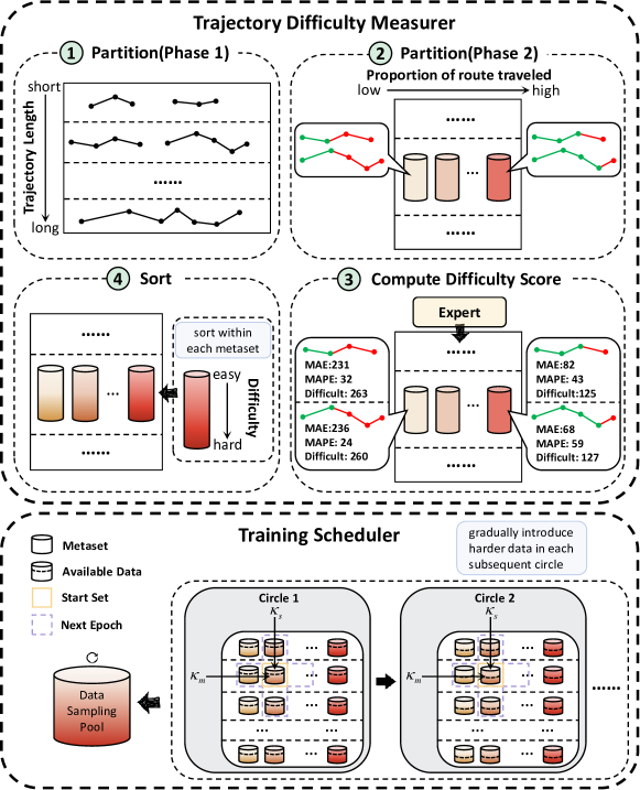
Figure 4. The Curriculum Learning Framework

In our proposed end-to-end training method, each trajectory may correspond to dozens of en route requests. Each request represents a new data point due to its distinct traveled route, which leads to a significant increase in the volume of training data. Training with randomly shuffled data not only converges slowly but also tends to fall into suboptimal local minima. To mitigate this issue, we introduce curriculum learning to train the model in a meaningful sequence. Specifically, it comprises two components: the Trajectory Difficulty Measurer and the Training Scheduler. In the following sections, we will elaborate on these components in detail.

5.1. Trajectory Difficulty Measurer

The Trajectory Difficulty Measurer evaluates the difficulty of the training samples and ranks them from easiest to hardest. The difficulty of estimating travel time can be assessed based on various factors, such as the complexity of the routes and the variability of traffic conditions. However, the model’s performance on the data is of greater importance. So we use a model trained on randomly shuffled data as an expert to evaluate the difficulty of the data, employing metrics including MAE, MAPE.

Partition. The direct comparison of trajectory data poses significant challenges due to the wide variation in their lengths. Firstly, trajectories of different lengths contain distinct data patterns, reflecting varying levels of prediction difficulty. For instance, shorter trajectories may contain fewer driving behaviors, providing limited useful information for the model to learn from, whereas longer trajectories encapsulate more complex and diverse driving patterns, thereby substantially increasing the difficulty of accurate prediction. Secondly, we rely on the expert to evaluate trajectory difficulty using multiple metrics, however, these metrics vary considerably for trajectories of different remaining route lengths.

Given the aforementioned reasons, we argue that prior to conducting trajectory difficulty assessment, it is essential to partition the trajectory data. Hence, as illustrated in Fig. 4, we partition the trajectories in two phases, and separately group the data according to two factors: the route length and the proportion of the route traveled. First, we partition the dataset $D$ based on the length of the route into $N$ disjoint subsets, i.e., $D=\{\tilde{D}_{1},\tilde{D}_{2},\ldots,\tilde{D}_{N}\}$, where $\tilde{D}_{i}$ represents the $i$-th subset and $\tilde{D}_{i}\cap\tilde{D}_{j}=\emptyset,\forall i\neq j,i,j\in[1,N]$. Each subset is then further divided into $M$ metasets based on the proportion of the route traveled, i.e., $D=\{\tilde{D}_{ij}\mid i=1,2,\ldots,N;\;j=1,2,\ldots,M\}$. For clarity, in the following text, we refer to $\tilde{D}_{i}$ as a ”subset” and $\tilde{D}_{ij}$ as a ”metaset”.

Difficulty Assessment. After partitioning the trajectory data, difficulty assessment only needs to be conducted within each individual metaset. The difficulty score is defined as follows:

(8) $$\mu_{i}=\text{MAE}(\mathcal{M}_{e}(\mathbf{x}_{i}),\mathbf{y}_{i})+\text{MAPE}(\mathcal{M}_{e}(\mathbf{x}_{i}),\mathbf{y}_{i})$$

where $\mathbf{x}_{i}$ is the input, $\mathbf{y}_{i}$ is the ground truth, and $\mathcal{M}_{e}$ denotes the expert. In Fig. 4, we provide illustrative examples of the corresponding difficulty scores for trajectories within different metasets. MAE provides a direct reflection of the absolute error in expert evaluations, while MAPE captures relative error, offering a better measure of the prediction’s accuracy in relation to the true values. By combining both MAE and MAPE, we address the limitations of relying on a single metric, allowing for a more comprehensive assessment of trajectory difficulty across different magnitudes and scales. We then sort the trajectories based on their difficulty scores.

1

Input : training dataset $\mathbf{D}$, subset number $\mathbf{N}$, metaset number $\mathbf{M}$, the Predictor $\mathcal{M}_{p}$, start position $\kappa_{s}$ and $\kappa_{m}$, training circle $cr$, training epochs $ep$, tolerance for early stopping $\tau_{tol}$.

Output : parameters $\theta_{p}$, for the Predictor $\mathcal{M}_{p}$.

2

3 initialize $\theta_{p}$ with normal distribution;

4 for $m\leftarrow 1\ldots cr$ do

5    release the more challenging data within each metaset;

6    Add $\tilde{D}_{\kappa_{s}\kappa_{m}}$ to sampling pool;

7    for $i\leftarrow 1\ldots ep$ do

8       $\theta_{p}\leftarrow$ train the Predictor with the sampling pool;

9       update the Predictor with $\theta_{p}$;

10       if $i<\max\left(N-\kappa_{s},\ \kappa_{s}-1,\ M-\kappa_{m},\ \kappa_{m}-1\right)+1$ then

11          include the neighboring sets of all newly added sets;

12         

13      calculate validation loss $L_{val}$;

14       if $|L_{val}^{i}-L_{val}^{i-1}|<\tau_{tol}$ then

15          break;

16         

17      

18   

Algorithm 3 Training Scheduler for RLER-TTE

5.2. Training Scheduler

Since we have already ordered the data within each metaset, an important task of the Training Scheduler is to determine how to arrange the metaset $\tilde{D}_{ij}$ for training. A straightforward approach is to directly select the simpler data from all metasets and add it to the sampling pool. However, as we mentioned earlier, this approach overlooks the varying difficulty levels among different metasets. Therefore, we propose that the data from different metasets should be sequentially introduced into the sampling pool throughout the curriculum. Intuitively, we believe that training should begin with datasets of moderate length and a balanced proportion of the traveled route, as their driving behavior patterns are easier to learn. Additionally, starting with medium-length trajectories facilitates generalization to both shorter and longer routes.

As presented in Algorithm 3, we design a dual-loop training method. This approach initiates with the training circle, an outer loop that iterates through all metasets, starting by training on easier data drawn from these sets. As each subsequent cycle progresses, more challenging data is gradually introduced. Within each major cycle, we define two hyperparameters, $\kappa_{s}$ and $\kappa_{m}$, to determine the starting position of the metaset for training, denoted as $\tilde{D}_{\kappa_{s}\kappa_{m}}$. As illustrated in Figure 4, $\kappa_{s}$ is used to select a subset, while $\kappa_{m}$ specifies the position of this metaset within this subset. Due to the unsuitability of edge positions in the metaset matrix for initiating training, the values of these two parameters are chosen from a moderate range of positions.

The inner loop is defined by epochs. At the start of each epoch, data is randomly sampled from the Data Sampling Pool for training. After each training session, we expand the Sampling Pool by adding any neighboring metasets of the newly introduced metaset that have not yet been included. For example, if ($\tilde{D}_{ij}$) is added, we also include its neighbors ($\tilde{D}_{i\pm 1,j\pm 1}$). This process continues until all metasets are incorporated into the Sampling Pool. Finally, we apply an early stopping strategy—once the model has been trained sufficiently on the current data, we conclude the major cycle and move on to the next one.

In the specific scenario of ER-TTE, we first partition the dataset into multiple metasets to effectively manage the training data. Then, we evaluate the difficulty of the data from two perspectives: the length of the trajectories and the starting locations of requests along the routes, as well as the complexity of trajectory data for prediction using deep learning models. In the subsequent experimental section, we will thoroughly investigate the impact of curriculum learning parameters on the results.

6. EXPERIMENTS

In this section, we evaluate the effectiveness, efficiency, and scalability of our method RLER-TTE on three real-world datasets.

6.1. Experimental Setup

Table 2. Statistics of Datasets

	Chengdu	Xi’an	Porto
Travel routes	5.8M	3.4M	0.5M
Avg travel time (s)	500.65	757.07	479.12
Time interval	10/1–11/30, 2016	10/1–11/30, 2016	7/1, 2013–6/30, 2014
Avg # of points	180	205	36
Avg # of road segments	17	25	19
Avg length (meter)	3,477.85	4,143.17	2471.38

Datasets. (1) Road Networks. We utilize three road networks in our experiments: Chengdu Road Network (CRN), Xi’an Road Network (XRN), and Porto Road Network (PRN), which are all extracted from OpenStreetMap (Ope, 2024). CRN includes 3191 vertices and 9468 edges; XRN contains 4576 vertices and 12668 edges; PRN contains 2755 vertices and 5315 edges.

(2) Travel Route. The trajectory data for Chengdu and Xi’an were collected from 10/01/2016 to 11/30/2016, while the trajectory data for Porto were collected from 07/01/2013 to 06/30/2014. The Chengdu dataset contains 5.8 million trajectories, the Xi’an dataset comprises 3.4 million trajectories, and the Porto dataset includes 0.5 million trajectories. We apply a map matching algorithm to align the GPS trajectories with the corresponding road networks, thereby deriving the travel routes for the three datasets. Table 2 presents the statistics of these datasets, where Avg # of points indicates the average number of GPS points in each travel route, and Avg # of road segments represents the average number of road segments traversed by each travel route.

(3) Traffic Condition. To calculate the historical traffic conditions, we partition the trajectory data into time slots $\Delta T$, where $\Delta T$ is set to 5 minutes in our work. We compute various traffic speeds for each road segment under different time slots, such as the mean and median values. For each travel route, we consider $p$ past time slots as the traffic conditions for that trajectory.

(4) Background Information. We collect weather conditions and compile data on holidays, weekends, and rush-hour as background information. Weather information is gathered from the website (wea, 2024), and the weather conditions are categorized into 16 types.

(5) Training, Validation and Test. We partition the datasets based on the day of data collection. Specifically, the datasets are divided into training, validation, and test sets according to the ratios of 70%:10%:20%, respectively.

Baseline methods. We compare our models with six baseline methods:

• Avg: We accumulate historical trajectory data for each time slot on every link, and compute the average speed within that time slot. The computed averages across all time slots for each link are then used to predict the travel time.

• DeepTTE (Wang et al., 2018b): This is a spatio-temporal neural network. It first encodes the spatial information through Geo-Conv, then encodes the temporal information using LSTM, and employs multi-task learning to predict the travel time for the entire route.

• STANN (He et al., 2019): This is a spatio-temporal attentive neural network. It proposes an LSTM-based encoder–decoder architecture to explore spatio-temporal relationships and introduces an attention mechanism in the decoder.

• ConST (Fang et al., 2020): This is a spatio-temporal graph neural network. It proposes a graph attention mechanism to capture the spatial and temporal dependencies to estimate the travel time.

• SSML (Fang et al., 2021): This is a meta-learning model for ER-TTE. It constructs ER-TTE as a few-shot learning problem and proposes a model-based self-supervised meta-learning method to learn meta-knowledge for travel time estimation.

• MetaER-TTE (Fan et al., 2022): This is a state-of-the-art meta-learning model for ER-TTE. It proposes an adaptive meta-learning model based on MAML (Finn et al., 2017), providing different initialization parameters and learning rates for trajectories with various contextual information.

End-to-end Evaluation. Unlike previous approaches (Fang et al., 2021; Fan et al., 2022) that use a fixed proportion of traveled distance for offline model training and evaluation, we propose an end-to-end evaluation method. In this method, mirroring real-world online scenarios, prediction requests are initiated at regular intervals along each trajectory. For each travel route, the metrics corresponding to all requests are averaged to provide an overall evaluation of the model’s performance throughout the entire route.

Evaluation Metrics. We evaluate our proposed methods and baseline methods based on three metrics: RMSE (Root Mean Square Error), MAE (Mean Absolute Error) and MAPE (Mean Absolute Percent Error), which are widely used by the baselines we compare with. Specifically, suppose that the ground truth of the remaining route is represented as $\mathbf{y}=\{y_{r}^{i}\}$ and the predicted travel time is denoted as $\mathbf{\hat{y}}=\{\hat{y}_{r}^{i}\}$, these metrics are defined as: $RMSE(\mathbf{y},\mathbf{\hat{y}})=\sqrt{\frac{1}{N}\sum_{i=1}^{N}(y_{r}^{i}-\hat{y}_{r}^{i})^{2}}$; $MAE(\mathbf{y},\mathbf{\hat{y}})=\frac{1}{N}\sum_{i=1}^{N}\left|y_{r}^{i}-\hat{y}_{r}^{i}\right|$; $MAPE(\mathbf{y},\mathbf{\hat{y}})=\frac{1}{N}\sum_{i=1}^{N}\left|\frac{y_{r}^{i}-\hat{y}_{r}^{i}}{y_{r}^{i}}\right|$, where $N$ denotes the number of the requests included in a travel route. We calculate the average of these metrics across all travel routes to evaluate the performance of all methods. In addition to the three base performance metrics, we also compared an efficiency metric: MUR (Model Utilization Rate), defined as the proportion of prediction requests that required recalculation by the Predictor.

Experimental Settings. All deep learning methods were implemented with PyTorch 2.0.1 and Python 3.11.5, and trained with a Tesla V100 GPU. The platform ran on Ubuntu 18.04 OS. In addition, we used Adam (Kingma and Ba, 2015) as the optimization method with the mini-batch size of 512. The learning rate is set as 0.0001, and the training epoch is set as 100, and an early stopping mechanism is adopted. For the Double DQN, the experience replay buffer size is set to 500,000, the target network update step to 2,000, and the discount factor to 0.9.

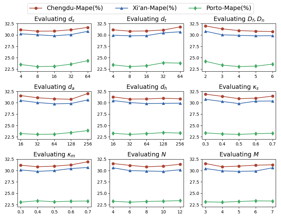
Figure 5. MAPE(%) vs. Hyper-parameters

6.2. Setting of Model’s Hyper-parameters

we consider the following hyper-parameters: (1) the embedding size ($d_{s}$, $d_{t}$) of road segments and time slots; (2) the depth ($D_{f}$, $D_{n}$) of the Offline Feature Encoder and Online Feature Encoder; (3) the settable-dimension size ($d_{a}$) of attention mechanism; (4) the settable-dimension size ($d_{h}$) of certain hidden representations; (5) the starting positions ($\kappa_{s}$, $\kappa_{m}$) for curriculum learning; (6) the partition sizes of the subset and metaset ($N$, $M$). In particular, given a hyper-parameter, we first select its value range according to the experience under some constraints (e.g., the limitation of GPU memory). Then, we conduct experiments on the validation Chengdu, Xi’an and Porto to determine its optimal value. As shown in Fig. 5, we plot the MAPE for different hyper-parameters. In summary, we set each hyper-parameter with the value corresponding to the optimal performance as follows: (1) For Chengdu, we have $d_{s}=8$, $d_{t}=8$, $D_{f}=6$, $D_{n}=6$, $d_{a}=128$, $d_{h}=32$, $\kappa_{s}=0.5$, $\kappa_{m}=0.4$, $N=8$, $M=4$. (2) For Xi’an, we have $d_{s}=16$, $d_{t}=8$, $D_{f}=5$, $D_{n}=5$, $d_{a}=64$, $d_{h}=64$, $\kappa_{s}=0.5$, $\kappa_{m}=0.4$, $N=10$, $M=5$. (3) For Porto, we have $d_{s}=8$, $d_{t}=8$, $D_{f}=4$, $D_{n}=4$, $d_{a}=32$, $d_{h}=32$, $\kappa_{s}=0.5$, $\kappa_{m}=0.3$, $N=6$, $M=4$.

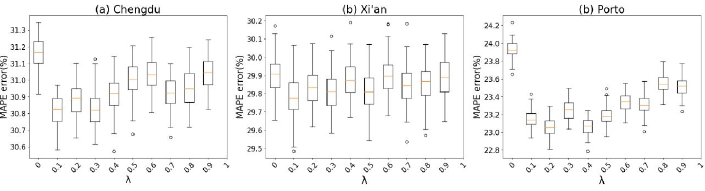
Figure 6. MAPE(%) vs. Loss Weight $\lambda$

6.3. Effectiveness of Loss Weight

To fine-tune the loss weight $\lambda$, we vary it from 0 to 1 in increments of 0.1 during the training of RLER-TTE. We compute the MAPE metric on the validation data and plot the corresponding box plots for the results of the three datasets in Figure 6. Our analysis indicates that performance significantly improves as $\lambda$ varies from 0 to 0.1, demonstrating the effectiveness of the contrastive learning module. However, as $\lambda$ increases further, the model’s performance generally exhibits a downward trend, indicating that the reinforcement learning loss becomes more critical and dominant. According to the majority voting rule, the optimal values of $\lambda$ for Chengdu, Xi’an, and Porto are 0.1, 0.1, and 0.2, respectively, which are set as the default values in subsequent experiments.

Table 3. Effectiveness Results on Test Data.

Dataset	Chengdu				Xi’an				Porto
Method	MAE (s)	RMSE (s)	MAPE (%)	MUR (%)	MAE (s)	RMSE (s)	MAPE (%)	MUR (%)	MAE (s)	RMSE (s)	MAPE (%)	MUR (%)
Avg	131.93	190.14	47.35	–	139.28	204.58	44.12	–	91.32	129.96	39.64	–
DeepTTE	120.78	167.85	43.15	100%	128.51	176.11	39.47	100%	69.92	94.09	29.86	100%
STANN	118.35	161.74	42.92	100%	129.67	174.63	39.86	100%	71.34	100.94	30.71	100%
ConST	112.36	143.18	41.26	100%	122.79	156.31	38.79	100%	68.16	92.07	28.83	100%
SSML	94.81	126.15	34.46	100%	106.43	140.89	33.02	100%	60.27	79.15	25.74	100%
MetaER-TTE	90.74	114.69	33.87	100%	103.81	134.09	31.49	100%	58.30	73.23	24.91	100%
ND	89.39	112.51	33.09	34.58%	101.38	129.97	30.94	35.44%	59.42	80.35	25.80	35.92%
NU	86.17	108.46	31.61	24.33%	98.23	125.61	30.42	25.67%	54.77	70.84	23.27	23.55%
NA	85.32	105.93	31.17	26.05%	96.97	122.49	29.87	26.71%	55.26	71.39	23.94	20.39%
RLER-TTE-s	90.83	115.92	33.79	29.64%	101.94	131.29	31.27	32.18%	56.93	75.87	24.16	27.86%
RLER-TTE-p	87.58	111.07	32.45	36.01%	100.72	128.26	31.05	31.59%	57.61	77.21	25.06	28.19%
RLER-TTE-a	91.81	121.73	34.38	42.76%	101.47	136.52	31.44	39.62%	56.74	74.65	24.53	34.02%
RLER-TTE	84.76	103.75	30.83	25.58%	96.59	121.68	29.81	24.36%	54.13	68.78	23.04	22.81%

6.4. Effectiveness Comparison

Apart from comparing RLER-TTE with baseline methods, we also propose three ablation study variants. In ND, we replace our proposed Double DQN network with a Transformer (Vaswani et al., 2017). All features are concatenated and then fed directly into the Transformer for decision-making. In NU, we remove the curriculum learning strategy and train the Predictor using all end-to-end data in a randomly shuffled order. In NA, we remove the contrastive loss and directly merge the online and offline features. To thoroughly investigate the role of the reinforcement learning agent in the framework, we further introduce agents based on the PPO (Schulman et al., 2017) method and the A3C (Mnih et al., 2016) method, integrated with the model architecture proposed in this paper, and denote them as RLER-TTE-p and RLER-TTE-a, respectively. All the aforementioned experiments use MetaER-TTE as the Predictor. Additionally, in RLER-TTE-s, we use SSML as the Predictor to demonstrate the robustness of our framework.

Table 3 reports the performance of all methods using different metrics on the three datasets, and we have the following observations:

(1) In end-to-end evaluation, the ER-TTE method demonstrates a significant performance improvement compared to the traditional TTE method, as its performance gradually enhances with the increase in the traveled distance. However, all methods exhibit relatively high MAPE values. This is attributed to the shortening of the remaining distance, which reduces the length of the trajectory to be predicted and consequently increases the relative percentage error.

(2) Avg performs worse compared to deep learning methods, because the former can approximately fit any function. Moreover, when historical data are sparse, the Avg method is insufficient for providing accurate predictions.

(3) In analyzing the results of the ablation experiments on ND, NU, and NA, we observed that the removal of the Double DQN network had the most significant impact, with a notable increase in both effective metrics and the MUR metric. This indicates that only using a single Transformer for decision-making is insufficient to capture the complex spatio-temporal correlation in online scenarios. The experiments on NU and NA demonstrate the effectiveness of our curriculum learning and contrastive learning components. While their impact on MUR was smaller, they still contributed to performance improvements.

(4) Comparing the experimental results of RLER-TTE-s and SSML, we find that our proposed framework is effective across multiple ER-TTE predictors, thereby demonstrating the robustness of our approach.

(5) The experimental results of RLER-TTE-p and RLER-TTE-a demonstrate that the Double DQN method exhibits superior performance in this scenario. This is primarily because Double DQN is better suited for reinforcement learning tasks that involve controlling discrete action spaces, especially when the number of actions is limited. In contrast, methods such as PPO and A3C are more appropriate for continuous action spaces. Given the relatively small action space in this task, the value-based Double DQN method can quickly learn the optimal Q-value for each action. While policy gradient-based methods, such as PPO and A3C, often result in overly complex policy optimization steps, which are more prone to instability and overfitting.

(6) RLER-TTE outperforms all other models across all metrics. This is attributed to our method’s analysis of driving behavior patterns, which selectively inputs beneficial real-time information into the Predictor, rather than feeding all newly observed data into the Predictor indiscriminately.

(7) The results of the MUR metric indicate that in real-world scenarios, the majority of real-time prediction requests do not necessitate re-computation by the estimated model. Compared to existing methods, our approach reduces the computational load by approximately fourfold, significantly enhancing the efficiency.

(8) When comparing the errors on the Chengdu and Xi’an datasets, all methods exhibit lower MAE and RMSE metrics on the Chengdu dataset, while the MAPE metric is relatively higher. This is primarily due to the shorter trajectories in the Chengdu dataset compared to those in Xi’an, resulting in smaller absolute errors but larger percentage errors when normalized by the overall trajectory length.

(9) The metrics on the Porto dataset are lower than Chengdu and Xi’an datasets. This is because the trajectories in the Porto dataset are shorter, and the GPS sampling frequency is lower, resulting in coarser granularity. These characteristics reduce the prediction difficulty for this dataset.

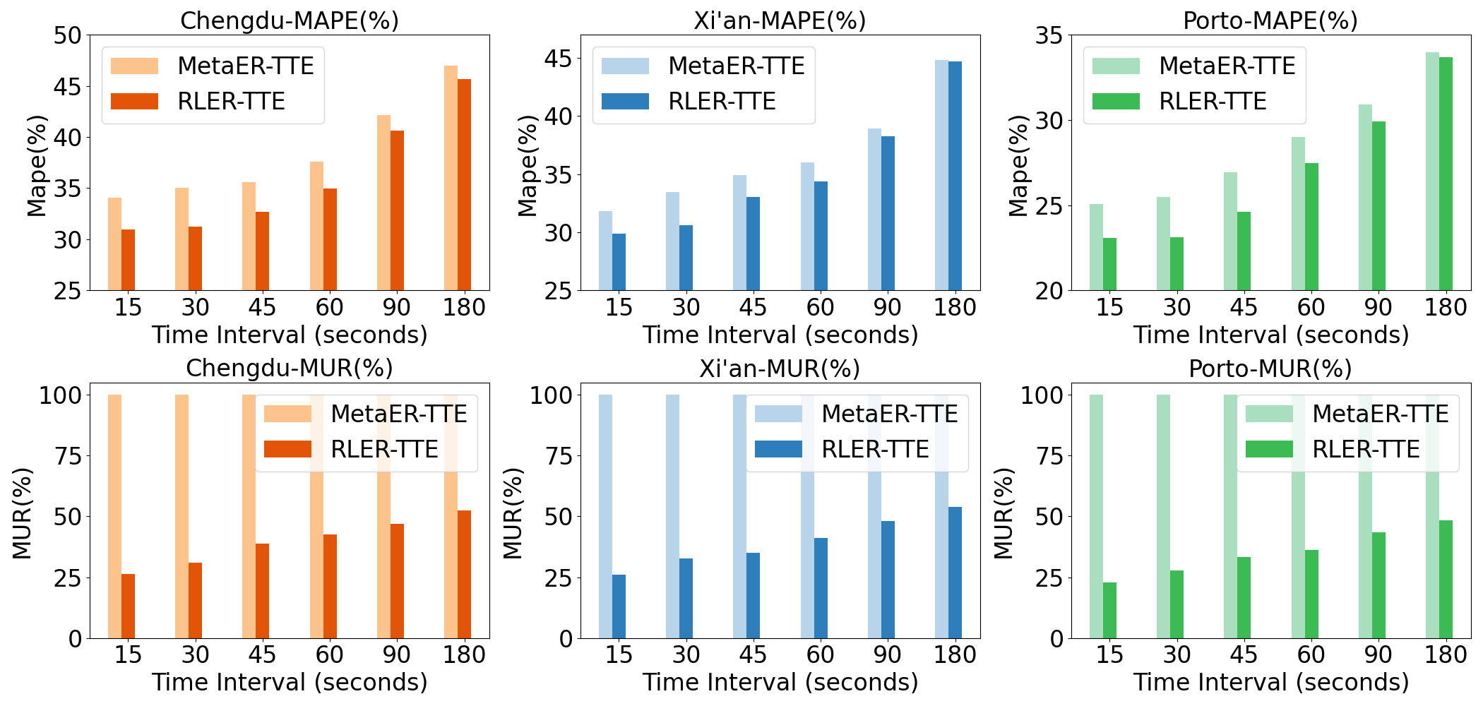
Figure 7. MAPE(%), MUR(%) vs. Time Interval

6.5. Effectiveness of Request Interval

The interval $\Delta t$ between real-time requests is a critical parameter for the online ER-TTE task, which has not been explored in previous work (Fang et al., 2021; Fan et al., 2022). To investigate the performance of our method under different values of $\Delta t$, we compare the MAPE and MUR metrics of RLER-TTE with the state-of-the-art method MetaER-TTE across various values of $\Delta t$, as shown in Figure 7. We summarize our findings as follows:

(1) As the time interval $\Delta t$ increases, the MAPE values of both methods rise accordingly. This indicates that more frequent en-route predictions lead to higher prediction accuracy.

(2) Our method demonstrates a consistent advantage over the baseline in terms of the MAPE metric across all intervals. However, as the prediction interval increases, the performance gains gradually diminish. This is due to the interval becoming excessively long relative to the trajectory. For instance, the average travel times in the Chengdu and Porto datasets are 500.65s and 479.12s, respectively. As the prediction interval increases, the number of en-route predictions decreases significantly, which is inconsistent with the application scenario of ER-TTE techniques and does not meet the requirements of real-world deployment systems.

(3) The MUR metric of RLER-TTE increases as $\Delta t$ grows, since a longer time interval implies that the newly collected real-time information at each prediction step is more valuable. Additionally, our frequency reward encourages the system to perform re-prediction when the duration of the previous prediction interval becomes longer. However, compared to the baseline method, our approach consistently maintains a significant improvement in the MUR metric, which greatly enhances efficiency.

Table 4. Efficiency of Different Methods

Method	memory size			training time			estimation latency
	(MByte)			(minutes/ep)			(seconds/K)
	Chengdu	Xi’an	Porto	Chengdu	Xi’an	Porto	Chengdu	Xi’an	Porto
Avg	183MB	126MB	21MB	-	-	-	-	-	-
DeepTTE	3.8MB	3.9MB	3.6MB	14.47	9.72	1.88	1.27s	1.53s	1.31s
STANN	6.4MB	6.5MB	6.1MB	5.59	3.41	0.73	0.61s	0.88s	0.65s
ConST	5.9MB	6.9MB	5.8MB	10.46	6.74	1.15	0.69s	0.93s	0.71s
SSML	6.2MB	7.4MB	5.9MB	16.22	12.68	2.07	1.19s	1.48s	1.26s
MetaER-TTE	7.1MB	8.0MB	6.4MB	13.34	8.41	1.35	0.78s	1.04s	0.86s
ND	5.7MB	6.8MB	5.1MB	7.91	4.83	0.82	0.35s	0.44s	0.38s
NU	6.8MB	8.9MB	6.4MB	11.35	7.29	1.16	0.29s	0.38s	0.28s
NA	6.8MB	8.8MB	6.3MB	11.24	7.08	1.13	0.30s	0.39s	0.27s
RLER-TTE-s	6.9MB	9.1MB	6.4MB	12.01	7.94	1.28	0.45s	0.59s	0.46s
RLER-TTE-p	9.1MB	13.6MB	6.8MB	10.39	6.18	1.07	0.39s	0.45s	0.40s
RLER-TTE-a	9.1MB	11.3MB	6.8MB	9.36	5.94	1.02	0.44s	0.56s	0.42s
RLER-TTE	6.8MB	8.9MB	6.4MB	11.47	7.22	1.17	0.29s	0.37s	0.27s

6.6. Efficiency Comparison

We compare efficiency in terms of memory usage, training time, and estimation latency. Memory usage measures the amount of memory consumed by each method to evaluate memory efficiency. Training time is used to compare the offline learning efficiency of deep learning-based methods, calculated as the average time per epoch for each method. Estimation latency assesses the efficiency of applying these methods in online scenarios. We selected 1,000 routes and evaluated the time required to perform complete real-time predictions with multiple real-time requests on these trajectories. The results are reported in Table 4. Our observations are as follows:

(1) The Avg method requires more memory compared to other approaches, as it needs to load data proportional to the size of the trajectory history, whereas other methods only need to load the model parameters.

(2) Due to the advantages of the attention mechanism, the training and estimation efficiency of STANN and ConST is higher. Meanwhile, the meta-learning components of SSML and MetaER-TTE contribute to an increased computational cost for these methods.

(3) Comparing the datasets of Xi’an, Chengdu and Porto, it is observed that the model parameters of the Xi’an dataset are more numerous. This is attributed to the larger road network in Xi’an. In contrast, the training time for the Chengdu dataset is longer, while that of Porto is much shorter due to differences in dataset sizes. Regarding estimation latency, the dataset from Xi’an requires a longer inference time compared to both Chengdu and Porto. This is because the trajectory lengths in Xi’an are generally longer.

(4) Our approach, RLER-TTE, achieves significantly better efficiency compared to prevailing state-of-the-art methods. This enhancement is primarily attributed to the efficiency of the lightweight reinforcement learning model, with the improvement ratio closely aligning with the model utilization rate of the Predictor within the framework.

(5) Comparing the results of ND, NU, and NA, we observe that the ND model requires fewer parameters and has a shorter training time due to its simpler architecture. On the other hand, NU and NA have a minimal impact on efficiency, as the system’s efficiency is primarily depends on the MUR metric. The primary purpose of these two components is to enhance the system’s performance, without compromising the framework’s inherent efficiency. The experimental results of RLER-TTE-p and RLER-TTE-a show that they consume more memory but deliver relatively inferior efficiency, further demonstrating that the double DQN method is better suited for the application scenario of our framework.

(6) The experimental results on RLER-TTE-s demonstrate that our framework possesses plug-and-play characteristics, allowing it to adapt to various estimated models. This robust generalization capability motivates us to explore more complex ER-TTE estimation methods. Moreover, more accurate models imply lower MUR, and with the aid of our framework, the efficiency cost can be significantly reduced.

Table 5. Scalability of methods, measured by MAPE(%)

Dataset	Chengdu/Xi’an
Scale	20%	40%	60%	80%	100%
Avg	58.78/55.34	52.43/49.15	49.12/46.03	48.12/44.89	47.35/44.12
DeepTTE	44.10/41.73	44.38/40.98	43.87/40.38	43.59/39.91	43.15/39.37
STANN	44.82/41.76	44.12/41.35	43.78/40.61	43.29/40.23	42.92/39.86
ConST	43.49/41.73	43.14/41.01	42.39/40.23	41.59/39.18	41.26/38.79
SSML	36.98/35.99	35.79/34.83	35.21/34.12	34.76/33.48	34.46/33.02
MetaER-TTE	37.23/35.61	35.41/33.76	34.52/32.72	34.01/31.83	33.47/31.49
RLER-TTE	33.97/33.41	32.64/31.85	31.98/30.97	31.35/30.28	30.83/29.81

6.7. Scalability Comparison

To evaluate the scalability of all methods, we train different models by varying the training data size. In particular, we sample 20%, 40%, 60%, 80% and 100% from the training data of Chengdu and Xi’an, and collect the associated MAPE of the online prediction over the test data, to more intuitively reflect the performance of the different methods. From Table 5, we have the following observations:

(1) As the volume of data increases, the performance of all methods improves, indicating that deep learning models have not yet reached their learning capacity limits. Larger datasets provide more diverse spatio-temporal information, which helps models better capture and understand the patterns and features in the data, thereby enhancing the models’ ability to generalize effectively.

(2) Deep learning methods are more stable and effective compared to Avg. For instance, the MAPE of Avg on the Chengdu dataset increases by $\frac{58.78-47.35}{47.35}=24.14\%$ when we only use 20% training data, while the ratio is only $\frac{33.97-30.83}{30.83}=10.18\%$ for RLER-TTE.

(3) Compared to all other baseline methods, our approach, RLER-TTE, consistently achieves the best performance across all scales of data.

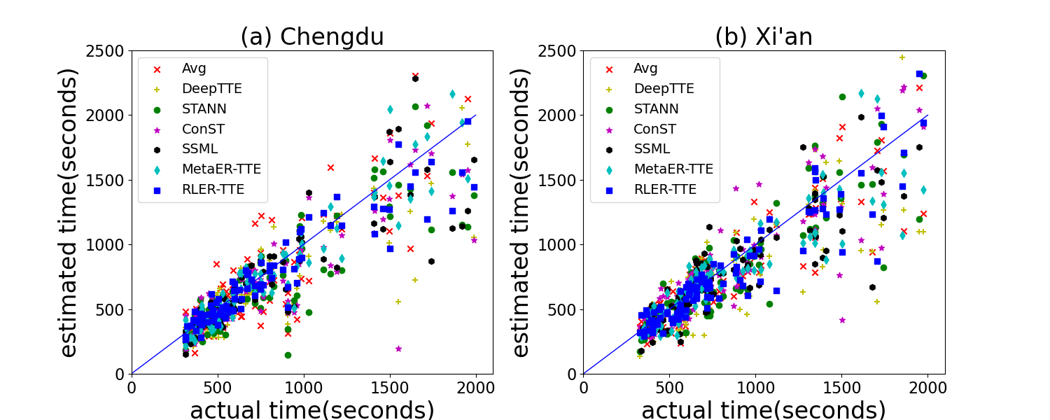
Figure 8. Estimated time vs. actual time.

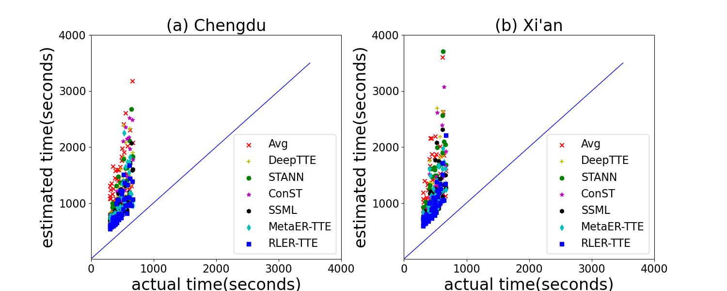
Figure 9. Estimated time vs. actual time on MAPE.

6.8. Case Study

To visually demonstrate the effectiveness of our framework, we employ scatter plots to compare all methods, with the $y$-axis representing the estimated time and the $x$-axis representing the actual time. As illustrated in Figure 8, we include a reference line $y=x$ for comparison. The closer the data points are to this reference line, the more accurate the predictions are. Conversely, the further the data points deviate from this line, the worse the performance of the method. We randomly sample 100 test data points from the Chengdu and Xi’an datasets. Our observations are as follows:

(1) The average error of the Avg method is generally larger but does not produce outliers with significantly high errors. In contrast, deep learning methods occasionally exhibit anomalous cases with substantial errors. (2) Across data of all lengths, our method, RLER-TTE, demonstrates closer adherence to the reference line compared to other methods. (3) As actual time increases, the errors for all methods grow, but RLER-TTE has the smallest degree of increase.

To evaluate the performance of each method under worst-case scenarios, we further select the 50 worst-performing instances for each method based on MAPE scores. These instances are plotted in a similarly formatted scatter plot in Figure 9. Since our selection is based on MAPE scores, shorter actual times result in larger relative errors, causing the majority of cases to cluster on the left side. Similarly, the performance of each method can be judged by the proximity of the data points to the reference line. We can find that:

(1) It is visually apparent that RLER-TTE adheres more closely to the reference line. (2) The Avg method performs worse in the worst-case scenario, with its errors being significantly larger than those of deep learning methods.

7. RELATED WORK

7.1. Travel Time Estimation

Travel Time Estimation (TTE) plays a crucial role in intelligent transportation systems, serving as the foundation for tasks such as traffic forecasting and navigation planning. Current research in this field can be broadly categorized into two types: offline travel time estimation and online travel time estimation.

Offline travel time estimation. Offline travel time estimation primarily involves learning and evaluation on datasets without considering real-time prediction scenarios. The mainstream studies can be primarily divided into two categories: OD-based and path-based. The OD-based methods (Jindal et al., 2017; Hu et al., 2016; Wang et al., 2019; Zhang et al., 2020; Li et al., 2018) take only the origin, destination locations, and departure times as inputs, and estimate the travel time for the corresponding OD pairs. Yuan et al. (Yuan et al., 2020) consider historical trajectory data associated with OD pairs and propose an efficient encoding technique based on neural networks, while Lin et al. (Lin et al., 2023) utilize diffusion models to further explore the complex relationships between trajectory data and OD pairs. However, these methods fail to capture the rich spatio-temporal information within the travel route, making it difficult to perform tasks such as navigation planning that require travel time estimation for a specified route. Therefore, the path-based methods (Wang et al., 2014; Zhang et al., 2018; Tran et al., 2020; Fang et al., 2020; Wang et al., 2022b; Yuan et al., 2022), which take a travel route as input, are proposed to address this issue. Luan et al. (Tran et al., 2020) consider future traffic information and propose a deep learning system that integrates both a future traffic flow prediction model and a travel time estimation model (Wang et al., 2018b). Zhao et al. (Liu et al., 2023) focus on aggregation operations in travel time estimation and design an Inverted Table to record aggregation requests. They propose a hierarchical reduction architecture suitable for multiple deep learning models. Yuan et al. (Yuan et al., 2022) focus on the unique correlations within link data, emphasizing characteristics such as heterogeneity and proximity between links. They treat traffic conditions as dynamic data, processing them separately from static link data. However, the so-called dynamic data is actually simulated based on different historical traffic conditions, making it essentially an offline attribute of the road network. Offline TTE studies typically perform prediction once before the journey begins, considering only the internal characteristics of static data in offline scenarios and primarily focusing on technical accuracy, while neglecting the real-time data collected during the journey in online scenarios. From a data perspective, our work emphasizes the characteristics of real-time data and the correlation between real-time and static data. Furthermore, we identify that real-time data exhibits characteristics such as unhelpful, misleading, and meaningless. Based on these findings, we innovatively propose an efficient online decision-making framework that redefines the data flow of the ER-TTE task and scientifically designs a Markov Decision Process to address this challenge.

Online Travel time estimation. Online travel time estimation is oriented towards online scenarios and is specifically designed to address the unique requirements of real-time environments. Kristin et al. (Tufte et al., 2007) proposed a stream-archive query system, which combines real-time traffic data streams and large transportation data archives for real-time travel time estimation. Lint et al. (van Lint, 2008) utilize simple neural networks to estimate travel time and employ the Extended Kalman Filter (EKF) to update the model weights online, enabling adaptation to changes in real-time traffic data. However, these methods are more reliant on the quality of historical data and lack the powerful capabilities of deep learning models. Therefore, Fu et al. (Fu et al., 2020) propose an online prediction framework consisting of a real-time prediction MLP and a sophisticated offline asynchronous updater. Han et al. (Han et al., 2023) introduce an incremental learning framework designed to continuously explore the spatio-temporal correlations present in new data. However, these methods only concentrate on the routes themselves and are merely extensions of offline methods applied in online scenarios, neglecting the user behavior patterns collected in real-time during the driving process. To address this problem, recent work has focused on en route travel time estimation. Fang et al. (Fang et al., 2021) first propose the ER-TTE task and formulate it as a few-shot learning problem, employing a model-based meta-learning approach to predict travel time. Fan et al. (Fan et al., 2022) improved upon meta-learning techniques by personalizing the initialization based on the unique context of each trajectory. However, existing methods fail to consider the complexity of real-world scenarios and do not sufficiently explore the relationship between driving behavior data and route data. Moreover, in the experimental settings, they only simulate a single request with a fixed traveled route, lacking a reasonable training and evaluation design. To address these issues, our work redefines the data pipeline and proposes a novel framework comprising a Decision Maker and a Predictor. Furthermore, we design comprehensive experiments and evaluations, establishing a new standard for the ER-TTE task.

7.2. Deep Learning in Spatio-Temporal Data

Recently, the remarkable performance of deep learning techniques in the field of spatio-temporal data management and mining has garnered attention. First, attention-based methods have shown advanced performance in capturing complex spatio-temporal correlations, with applications in areas such as Next POI Recommendation (Luo et al., 2021; Jiang et al., 2024) and traffic flow prediction (Yuan et al., 2021; Zheng et al., 2021; Chen et al., 2024; Yuan and Li, 2021). Second, an increasing number of methods employ Graph Neural Networks (GNNs) and hybrid architectures combining various neural networks to analyze spatio-temporal data. For example, Yuan et al. (Yuan et al., 2024) utilized GNNs and RNNs to capture spatio-temporal correlations for Traffic Speed Histogram Imputation, while Wu et al. (Wu et al., 2023) used Graph Convolution Networks (GCNs) and Graph Isomorphism Networks (GINs) to extract temporal dependencies within time series and spatial correlations between different time series for effective time series prediction. Last but not least, numerous deep learning approaches based on other architectures have also been applied to spatio-temporal data processing. For instance, Ahuja et al. (Ahuja et al., 2023) employ Variational Auto Encoders (VAE) to handle the release and denoising of spatio-temporal data, capturing and reconstructing complex spatio-temporal patterns.

8. CONCLUSION

This paper has introduced RLER-TTE, a novel and efficient framework designed to address the complex challenge of en route travel time estimation. Firstly, we redefined the implementation path of ER-TTE, proposing for the first time a novel pipeline comprising a Decision Maker and a Predictor. Next, we meticulously designed a Markov Decision Process and deployed efficient reinforcement learning to achieve effective autonomous decision-making in dynamic online environments. Furthermore, we established the training and evaluation standards for ER-TTE and introduced a curriculum learning strategy to manage the large volume of training data. Extensive experiments on real-world datasets validated the effectiveness, efficiency, and robustness of our model.

- (1)
- wea (2024) 2024. https://www.tianqi5.cn/lishitianqi/
- Ope (2024) 2024. OpenStreetMap. https://www.openstreetmap.org
- Ahuja et al. (2023) Ritesh Ahuja, Sepanta Zeighami, Gabriel Ghinita, and Cyrus Shahabi. 2023. A Neural Approach to Spatio-Temporal Data Release with User-Level Differential Privacy. In SIGMOD, Vol. 1. 21:1–21:25.
- Brakatsoulas et al. (2005) Sotiris Brakatsoulas, Dieter Pfoser, Randall Salas, and Carola Wenk. 2005. On Map-Matching Vehicle Tracking Data. In VLDB, Klemens Böhm, Christian S. Jensen, Laura M. Haas, Martin L. Kersten, Per-Åke Larson, and Beng Chin Ooi (Eds.). ACM, 853–864.
- Chen et al. (2024) Minxiao Chen, Haitao Yuan, Nan Jiang, Zhifeng Bao, and Shangguang Wang. 2024. Urban Traffic Accident Risk Prediction Revisited: Regionality, Proximity, Similarity and Sparsity. In Proceedings of the 33rd ACM International Conference on Information and Knowledge Management, CIKM 2024, Boise, ID, USA, October 21-25, 2024. ACM, 281–290.
- Fan et al. (2022) Yu Fan, Jiajie Xu, Rui Zhou, Jianxin Li, Kai Zheng, Lu Chen, and Chengfei Liu. 2022. MetaER-TTE: An Adaptive Meta-learning Model for En Route Travel Time Estimation. In IJCAI, Luc De Raedt (Ed.). ijcai.org, 2023–2029.
- Fang et al. (2021) Xiaomin Fang, Jizhou Huang, Fan Wang, Lihang Liu, Yibo Sun, and Haifeng Wang. 2021. SSML: Self-Supervised Meta-Learner for En Route Travel Time Estimation at Baidu Maps. In SIGKDD, Feida Zhu, Beng Chin Ooi, and Chunyan Miao (Eds.). ACM, 2840–2848.
- Fang et al. (2020) Xiaomin Fang, Jizhou Huang, Fan Wang, Lingke Zeng, Haijin Liang, and Haifeng Wang. 2020. ConSTGAT: Contextual Spatial-Temporal Graph Attention Network for Travel Time Estimation at Baidu Maps. In SIGKDD, Rajesh Gupta, Yan Liu, Jiliang Tang, and B. Aditya Prakash (Eds.). ACM, 2697–2705.
- Finn et al. (2017) Chelsea Finn, Pieter Abbeel, and Sergey Levine. 2017. Model-Agnostic Meta-Learning for Fast Adaptation of Deep Networks. In ICML (Proceedings of Machine Learning Research, Vol. 70), Doina Precup and Yee Whye Teh (Eds.). PMLR, 1126–1135.
- Fu et al. (2020) Kun Fu, Fanlin Meng, Jieping Ye, and Zheng Wang. 2020. CompactETA: A Fast Inference System for Travel Time Prediction. In SIGKDD, Rajesh Gupta, Yan Liu, Jiliang Tang, and B. Aditya Prakash (Eds.). ACM, 3337–3345.
- Grover and Leskovec (2016) Aditya Grover and Jure Leskovec. 2016. node2vec: Scalable Feature Learning for Networks. In SIGKDD, Balaji Krishnapuram, Mohak Shah, Alexander J. Smola, Charu C. Aggarwal, Dou Shen, and Rajeev Rastogi (Eds.). ACM, 855–864.
- Han et al. (2023) Jindong Han, Hao Liu, Shui Liu, Xi Chen, Naiqiang Tan, Hua Chai, and Hui Xiong. 2023. iETA: A Robust and Scalable Incremental Learning Framework for Time-of-Arrival Estimation. In SIGKDD, Ambuj K. Singh, Yizhou Sun, Leman Akoglu, Dimitrios Gunopulos, Xifeng Yan, Ravi Kumar, Fatma Ozcan, and Jieping Ye (Eds.). ACM, 4100–4111.
- He et al. (2019) Zhixiang He, Chi-Yin Chow, and Jia-Dong Zhang. 2019. STANN: A Spatio-Temporal Attentive Neural Network for Traffic Prediction. In IEEE Access, Vol. 7. 4795–4806.
- Hu et al. (2016) Huiqi Hu, Guoliang Li, Zhifeng Bao, Jianhua Feng, Yongwei Wu, Zhiguo Gong, and Yaoqiang Xu. 2016. Top-k spatio-textual similarity join. In ICDE. IEEE Computer Society, 1576–1577.
- Jiang et al. (2024) Nan Jiang, Haitao Yuan, Jianing Si, Minxiao Chen, and Shangguang Wang. 2024. Towards Effective Next POI Prediction: Spatial and Semantic Augmentation with Remote Sensing Data. In ICDE. IEEE, 5061–5074.
- Jindal et al. (2017) Ishan Jindal, Zhiwei (Tony) Qin, Xue-wen Chen, Matthew S. Nokleby, and Jieping Ye. 2017. A Unified Neural Network Approach for Estimating Travel Time and Distance for a Taxi Trip. CoRR abs/1710.04350 (2017).
- Kingma and Ba (2015) Diederik P. Kingma and Jimmy Ba. 2015. Adam: A Method for Stochastic Optimization. In ICLR, Yoshua Bengio and Yann LeCun (Eds.).
- Li et al. (2018) Yaguang Li, Kun Fu, Zheng Wang, Cyrus Shahabi, Jieping Ye, and Yan Liu. 2018. Multi-task Representation Learning for Travel Time Estimation. In SIGKDD, Yike Guo and Faisal Farooq (Eds.). ACM, 1695–1704.
- Lin et al. (2023) Yan Lin, Huaiyu Wan, Jilin Hu, Shengnan Guo, Bin Yang, Youfang Lin, and Christian S. Jensen. 2023. Origin-Destination Travel Time Oracle for Map-based Services. In SIGMOD, Vol. 1. 217:1–217:27.
- Liu et al. (2023) Zhao Liu, Mengquan Li, Mincan Li, Lei Liao, and Kenli Li. 2023. An Efficient Hierarchical-Reduction Architecture for Aggregation in Route Travel Time Estimation. In TPDS, Vol. 34. 2541–2552.
- Luo et al. (2021) Yingtao Luo, Qiang Liu, and Zhaocheng Liu. 2021. STAN: Spatio-Temporal Attention Network for Next Location Recommendation. In WWW, Jure Leskovec, Marko Grobelnik, Marc Najork, Jie Tang, and Leila Zia (Eds.). ACM / IW3C2, 2177–2185.
- Mnih et al. (2016) Volodymyr Mnih, Adrià Puigdomènech Badia, Mehdi Mirza, Alex Graves, Timothy P. Lillicrap, Tim Harley, David Silver, and Koray Kavukcuoglu. 2016. Asynchronous Methods for Deep Reinforcement Learning. In ICML (JMLR Workshop and Conference Proceedings, Vol. 48), Maria-Florina Balcan and Kilian Q. Weinberger (Eds.). JMLR.org, 1928–1937.
- Schulman et al. (2017) John Schulman, Filip Wolski, Prafulla Dhariwal, Alec Radford, and Oleg Klimov. 2017. Proximal Policy Optimization Algorithms. In CoRR, Vol. abs/1707.06347.
- Tan et al. (2023) Cheng Tan, Zhangyang Gao, Lirong Wu, Yongjie Xu, Jun Xia, Siyuan Li, and Stan Z. Li. 2023. Temporal Attention Unit: Towards Efficient Spatiotemporal Predictive Learning. In CVPR. IEEE, 18770–18782.
- Tran et al. (2020) Luan V. Tran, Minyoung Mun, Matthew Lim, Jonah Yamato, Nathan Huh, and Cyrus Shahabi. 2020. DeepTRANS: A Deep Learning System for Public Bus Travel Time Estimation using Traffic Forecasting. In VLDB, Vol. 13. 2957–2960.
- Tufte et al. (2007) Kristin Tufte, Jin Li, David Maier, Vassilis Papadimos, Robert L. Bertini, and James Rucker. 2007. Travel time estimation using NiagaraST and latte. In SIGMOD, Chee Yong Chan, Beng Chin Ooi, and Aoying Zhou (Eds.). ACM, 1091–1093.
- van Hasselt et al. (2016) Hado van Hasselt, Arthur Guez, and David Silver. 2016. Deep Reinforcement Learning with Double Q-Learning. In AAAI, Dale Schuurmans and Michael P. Wellman (Eds.). AAAI Press, 2094–2100.
- van Lint (2008) J. W. C. van Lint. 2008. Online Learning Solutions for Freeway Travel Time Prediction. In TITS, Vol. 9. 38–47.
- Vaswani et al. (2017) Ashish Vaswani, Noam Shazeer, Niki Parmar, Jakob Uszkoreit, Llion Jones, Aidan N. Gomez, Lukasz Kaiser, and Illia Polosukhin. 2017. Attention is All you Need. In NIPS. 5998–6008.
- Wang et al. (2022b) Chenxing Wang, Fang Zhao, Haichao Zhang, Haiyong Luo, Yanjun Qin, and Yuchen Fang. 2022b. Fine-Grained Trajectory-Based Travel Time Estimation for Multi-City Scenarios Based on Deep Meta-Learning. In TITS, Vol. 23. 15716–15728.
- Wang et al. (2018b) Dong Wang, Junbo Zhang, Wei Cao, Jian Li, and Yu Zheng. 2018b. When Will You Arrive? Estimating Travel Time Based on Deep Neural Networks. In AAAI, Sheila A. McIlraith and Kilian Q. Weinberger (Eds.). AAAI Press, 2500–2507.
- Wang et al. (2019) Hongjian Wang, Xianfeng Tang, Yu-Hsuan Kuo, Daniel Kifer, and Zhenhui Li. 2019. A Simple Baseline for Travel Time Estimation using Large-scale Trip Data. In TITS, Vol. 10. 19:1–19:22.
- Wang et al. (2022a) Yong Wang, Guoliang Li, Kaiyu Li, and Haitao Yuan. 2022a. A Deep Generative Model for Trajectory Modeling and Utilization. Proc. VLDB Endow. 16, 4 (2022), 973–985.
- Wang et al. (2014) Yilun Wang, Yu Zheng, and Yexiang Xue. 2014. Travel time estimation of a path using sparse trajectories. In SIGKDD, Sofus A. Macskassy, Claudia Perlich, Jure Leskovec, Wei Wang, and Rayid Ghani (Eds.). ACM, 25–34.
- Wang et al. (2018a) Zheng Wang, Kun Fu, and Jieping Ye. 2018a. Learning to Estimate the Travel Time. In SIGKDD, Yike Guo and Faisal Farooq (Eds.). ACM, 858–866.
- Wenk et al. (2006) Carola Wenk, Randall Salas, and Dieter Pfoser. 2006. Addressing the Need for Map-Matching Speed: Localizing Globalb Curve-Matching Algorithms. In SSDBM. IEEE Computer Society, 379–388.
- Wu et al. (2023) Xinle Wu, Dalin Zhang, Miao Zhang, Chenjuan Guo, Bin Yang, and Christian S. Jensen. 2023. AutoCTS+: Joint Neural Architecture and Hyperparameter Search for Correlated Time Series Forecasting. In SIGMOD, Vol. 1. 97:1–97:26.
- Yuan et al. (2024) Haitao Yuan, Gao Cong, and Guoliang Li. 2024. Nuhuo: An Effective Estimation Model for Traffic Speed Histogram Imputation on A Road Network. In VLDB, Vol. 17. 1605–1617.
- Yuan and Li (2019) Haitao Yuan and Guoliang Li. 2019. Distributed In-memory Trajectory Similarity Search and Join on Road Network. In ICDE. IEEE, 1262–1273.
- Yuan and Li (2021) Haitao Yuan and Guoliang Li. 2021. A Survey of Traffic Prediction: from Spatio-Temporal Data to Intelligent Transportation. Data Sci. Eng. 6, 1 (2021), 63–85.
- Yuan et al. (2022) Haitao Yuan, Guoliang Li, and Zhifeng Bao. 2022. Route Travel Time Estimation on A Road Network Revisited: Heterogeneity, Proximity, Periodicity and Dynamicity. In VLDB, Vol. 16. 393–405.
- Yuan et al. (2020) Haitao Yuan, Guoliang Li, Zhifeng Bao, and Ling Feng. 2020. Effective Travel Time Estimation: When Historical Trajectories over Road Networks Matter. In SIGMOD, David Maier, Rachel Pottinger, AnHai Doan, Wang-Chiew Tan, Abdussalam Alawini, and Hung Q. Ngo (Eds.). ACM, 2135–2149.
- Yuan et al. (2021) Haitao Yuan, Guoliang Li, Zhifeng Bao, and Ling Feng. 2021. An Effective Joint Prediction Model for Travel Demands and Traffic Flows. In ICDE. IEEE, 348–359.
- Zhang et al. (2018) Hanyuan Zhang, Hao Wu, Weiwei Sun, and Baihua Zheng. 2018. DeepTravel: a Neural Network Based Travel Time Estimation Model with Auxiliary Supervision. In IJCAI, Jérôme Lang (Ed.). ijcai.org, 3655–3661.
- Zhang et al. (2020) Wen Zhang, Yang Wang, Xike Xie, Chuancai Ge, and Hengchang Liu. 2020. Real-time Travel Time Estimation with Sparse Reliable Surveillance Information. In Proc. ACM Interact. Mob. Wearable Ubiquitous Technol., Vol. 4. 36:1–36:23.
- Zheng et al. (2021) Haifeng Zheng, Feng Lin, Xinxin Feng, and Youjia Chen. 2021. A Hybrid Deep Learning Model With Attention-Based Conv-LSTM Networks for Short-Term Traffic Flow Prediction. In TITS, Vol. 22. 6910–6920.