PhoTorch: A robust and generalized biochemical photosynthesis model fitting package based on PyTorch

Abstract

Advancements in artificial intelligence (AI) have greatly benefited plant phenotyping and predictive modeling. However, unrealized opportunities exist in leveraging AI advancements in model parameter optimization for parameter fitting in complex biophysical models. This work developed novel software, PhoTorch, for fitting parameters of the Farquhar, von Caemmerer, and Berry (FvCB) biochemical photosynthesis model based the parameter optimization components of the popular AI framework PyTorch. The primary novelty of the software lies in its computational efficiency, robustness of parameter estimation, and flexibility in handling different types of response curves and sub-model functional forms. PhoTorch can fit both steady-state and non-steady-state gas exchange data with high efficiency and accuracy. Its flexibility allows for optional fitting of temperature and light response parameters, and can simultaneously fit light response curves and standard $A/C_{i}$ curves. These features are not available within presently available $A/C_{i}$ curve fitting packages. Results illustrated the robustness and efficiency of PhoTorch in fitting $A/C_{i}$ curves with high variability and some level of artifacts and noise. PhoTorch is more than four times faster than benchmark software, which may be relevant when processing many non-steady-state $A/C_{i}$ curves with hundreds of data points per curve. PhoTorch provides researchers from various fields with a reliable and efficient tool for analyzing photosynthetic data. The Python package is openly accessible from the repository: https://github.com/GEMINI-Breeding/photorch.

1 Introduction

The Farquhar, von Caemmerer, and Berry (FvCB) model (Farquhar et al., 1980) is a widely used biochemically-based framework for describing the photosynthetic response of $C_{3}$ plants to intercellular CO₂ concentration, with more recent variations including the impacts of light, temperature, and water status, among others. This model, along with its many modified versions, defines numerous physiologically-based parameters that can be used to describe the response of photosynthesis to environmental variables (Farquhar et al., 1980; Harley et al., 1992; Medlyn et al., 2002; Sharkey et al., 2007). The extracted parameters are often used as quasi-traits in plant physiology, crop modeling, ecological modeling, and climate change research due to their mechanistic linkage to physiological processes (Martinez and Fridley, 2018; Kim et al., 2020; Li et al., 2021; Shin et al., 2021; Xue et al., 2022).

The FvCB model parameters cannot be directly measured in isolation, but are instead typically inferred by fitting the FvCB model to photosynthetic response curves. This means that, in addition to measurement errors, errors can also be incurred from the model fitting procedure. Challenges inherent in fitting the FvCB to experimental response curves have been explored extensively in prior literature (e.g., Long and Bernacchi, 2003; Miao et al., 2009; Gu et al., 2010; Busch et al., 2024). These challenges arise due to the fact that the model is over-parameterized, and is a switch-type equation with discontinuous transitions between states. This can create situations in which different combinations of model parameters result in similar fitting errors, and can make fitted values sensitive to initial parameter guesses.

Currently available packages that specialize in fitting the FvCB model, which mitigate associated fitting challenges to some extent, include FitFarquharModel (De Kauwe et al., 2016), plantecophys (Duursma, 2015), “photosynthesis” (Stinziano et al., 2021), and various Excel-based routines (Sharkey et al., 2007; Bellasio et al., 2016). Limitations of current models or packages include the inability to fit TPU parameters (De Kauwe et al., 2016) and the inability to fit light and temperature response parameters simultaneously (Duursma, 2015; Stinziano et al., 2021). These packages do not provide fitting for a comprehensive set of CO₂, light and temperature response parameters, and thus they may need to assume some parameters are conserved across different species or genotypes, even though parameter variability exists (Wieloch et al., 2023; Busch et al., 2024). Excel-based models lack computational efficiency and flexibility, and can be highly sensitive to initial parameter guesses (Dubois et al., 2007). These Excel-based methods also require users to specify the transition point from RuBP-saturated to RuBP-limited photosynthesis rate (Busch et al., 2024). Additionally, these packages were intended for use with steady-state $A/C_{i}$ response data, while more recent instruments allow for $A/C_{i}$ curve estimation based on non-steady-state data (Stinziano et al., 2017; Taylor and Long, 2019; Stinziano et al., 2019; Saathoff and Welles, 2021; Tejera-Nieves et al., 2024). As result, these packages can have long runtimes for dense non-steady-state $A/C_{i}$ data, although this can be mitigated by downsampling the steady-state data to use fewer data points (Burnett et al., 2019), with the trade-off being the accuracy of parameter estimation. Therefore, developing new $A/C_{i}$ curve fitting tools that can fit both steady-state and non-steady-state gas exchange response data, while also providing additional flexibility for fitting light and temperature response parameters, is of potential value to the community.

Advancements in artificial intelligence have also led to advancements in its related sub-disciplines, such as in efficient and robust parameter calibration within complex models. Artificial intelligence is effectively a parameter optimization problem, where the goal is to determine the values of thousands or millions of parameters that allow the model to optimally fit the training data. These parameter optimization routines have more generalized potential to improve parameter fitting in complex biophysical models.

Generalized frameworks providing a computational foundation for implementing AI models have emerged, such as the Python-based package PyTorch (Paszke et al., 2019). As one of the most popular deep learning frameworks, PyTorch offers many highly optimized standard functions with high computational performance on both CPU and GPU hardware. Thus, encoding the FvCB model in PyTorch and treating it as a deep learning model, with the physiological parameters as adjustable weights, is both reasonable and feasible. The optimization of FvCB model parameters can utilize advanced features provided by PyTorch, such as automatic differentiation and flexible enforcement of constraints.

This work developed a new tool named PhoTorch based on PyTorch for determination of parameters of the biochemical FvCB photosynthesis model based on leaf-level gas exchange data. In addition to reliable parameter estimation, novel aspects of the tool include its flexibility in fitting to CO₂, light, and temperature response data, inclusion of multiple light and temperature functions, and ability to handle noisy data or data with artifacts in some cases. It can handle both non-steady-state and steady-state $A/C_{i}$ curves with high efficiency. These benefits are achieved through careful regulation of the optimization process and the full utilization of PyTorch’s automatic differentiation and the computational efficiency of the Adam optimizer. The goal is to provide a user-friendly, open-source tool for accurately estimating photosynthetic parameters that improves users’ ability to model photosynthetic responses under various temperature and light conditions.

2 Materials and methods

2.1 FvCB model with light and temperature response functions

The goal of the PhoTorch software is to estimate parameters in the FvCB model based on input leaf-level gas exchange data. This section describes the theory and forms of the FvCB used by PhoTorch, and the associated model parameters. The FvCB model describes the rate of photosynthesis as being limited by the rate of ribulose-1,5-bisphosphate carboxylase/oxygenase (Rubisco) carboxylation, the rate of ribulose-1,5-bisphosphate (RuBP) regeneration, or the rate of triose-phosphate utilization (TPU). The general model form used herein is based on that of Harley et al. (1992) with two possible light response functions and two possible temperature response functions, and with the option of fitting the mesophyll conductance ($g_{m}$), as in many prior studies (Ethier and Livingston, 2004). The net rate of photosynthesis ($A$) on a per leaf area basis is calculated according to:

$$A=\min(W_{c},W_{j},W_{p})(1-\frac{\Gamma^{*}}{C_{i}})-R_{d},$$ (1)

where $R_{d}$ ($\mu$mol/m²/s) is the dark respiration rate, $\Gamma^{*}$ ($\mu$mol/mol) is the CO₂ compensation point when mitochondrial respiration is zero, and $C_{i}$ ($\mu$mol/mol) is the intercellular CO₂ concentration.

The rate of carboxylation limited by the amount, activation state, and kinetic properties of Rubisco ($W_{c}$) is given by:

$$W_{c}=\frac{V_{cmax}C_{i}}{C_{i}+K_{c}\left(1+\frac{O}{K_{o}}\right)},$$ (2)

where $V_{cmax}$ ($\mu$mol/m²/s) is the maximum rate of carboxylation, $K_{c}$ ($\mu$mol/mol) and $K_{o}$ (mmol/mol) are the Michaelis-Menten constants for carboxylation and oxygenation, respectively, and $O$ (mmol/mol) is the oxygen concentration.

The rate of carboxylation limited solely by the RuBP regeneration ($W_{j}$) is described by:

$$W_{j}=\frac{JC_{i}}{4(C_{i}+2\Gamma^{*})},$$ (3)

where $J$ ($\mu$mol/m²/s) is the CO₂ saturated electron transport rate. Its response to the incoming photosynthetic photon flux density (PPFD) can be described using a rectangular hyperbola (Farquhar et al., 1980):

$$J=\frac{\alpha QJ_{max}}{\alpha Q+J_{max}},$$ (4)

where $\alpha$ is the quantum yield of electron transport, $Q$ ($\mu$mol/m²/s) is the absorbed PPFD, and $J_{max}$ is the maximum rate of electron transport. A non-rectangular hyperbolic function (Medlyn et al., 2002) is more widely used to describe the relationship between $J$ and PPFD:

$$J=\frac{\alpha Q+J_{max}-\sqrt{(\alpha Q+J_{max})^{2}-4\theta\alpha QJ_{max}}}{2\theta},$$ (5)

where $\theta$ is the curvature parameter. Note that as $\theta$ approaches zero, Eqs. 4 and 5 become equivalent.

In the model fitting code, users have the option to use Eq. 4 (rectangular hyperbola) or Eq. 5 (non-rectangular hyperbola), and are referenced respectively as light response type 1 and 2. If the light response type is set to 0, $J$ is always equal to $J_{max}$.

The rate of carboxylation limited by inorganic phosphate ($W_{p}$) is given by:

$$W_{p}=3\mathrm{TPU}\frac{C_{i}}{C_{i}-(1+3\alpha_{g})\Gamma^{*}},$$ (6)

where $\mathrm{TPU}$ ($\mu$mol/m²/s) is the rate of triose phosphate utilization, and $\alpha_{g}$ is the stoichiometric ratio of orthophosphate (P_i) consumption in oxygenation (Von Caemmerer, 2000; Ellsworth et al., 2015).

If the user includes fitting of mesophyll conductance $g_{m}$, then the above-mentioned $C_{i}$ is replaced with chloroplastic CO₂ concentration $C_{c}$ according to:

$$C_{c}=C_{i}-A/g_{m}.$$ (7)

The temperature responses of four main parameters $V_{cmax}$, $J_{max}$, $\mathrm{TPU}$, and $R_{d}$ of the FvCB model can be represented according to the Arrhenius function (Medlyn et al., 2002):

$$k=k_{25}\exp{\left[\frac{\Delta{H_{a}}}{R}\left(\frac{1}{298}-\frac{1}{T_{leaf}}\right)\right]},$$ (8)

which results in monotonic increase in the parameter ($k$ being one of $V_{cmax}$, $J_{max}$, $\mathrm{TPU}$, or $R_{d}$, and $k_{25}$ is the value of the corresponding parameter at 25^∘C) with leaf temperature $T_{leaf}$ (Kelvin). A more flexible temperature response function can also be used that can represent a temperature optimum:

$$k=k_{25}\exp\left[\frac{\Delta H_{a}}{R}\left(\frac{1}{298}-\frac{1}{T_{leaf}}\right)\right]\frac{f\left(298\right)}{f\left(T_{leaf}\right)},$$ (9)

$$f(T)=1+\exp\left[\frac{\Delta H_{d}}{R}\left(\frac{1}{T_{opt}}-\frac{1}{T}\right)-\ln\left(\frac{\Delta H_{d}}{\Delta H_{a}}-1\right)\right]$$ (10)

where $\Delta{H_{a}}$ is the activation energy (kJ/mol), $\Delta{H_{d}}$ is the deactivation energy (kJ/mol), $T_{opt}$ is the temperature in Kelvin at which $k$ is optimal, and $R$ is the universal gas constant (0.008314 KJ/mol/K).

$K_{c}$, $K_{o}$, and $\Gamma^{*}$ can be directly calculated based on Eq. 8 using their corresponding $k_{25}$ and $\Delta{H_{a}}$ values reported by (Bernacchi et al., 2001), or they can be directly fitted using PhoTorch. It should be noted that the parameter $c$ used in the temperature response function of Bernacchi et al. (2001) is a scaling constant, which is equal to $\frac{\Delta H_{a}}{298R}+\ln{k_{25}}$, and thus can be substituted for and omitted as a parameter. In the code, the temperature response types 1 and 2 correspond to Eq. 8 and 9, respectively. If the temperature response type is set to 0, $V_{cmax}$, $J_{max}$, $\mathrm{TPU}$, and $R_{d}$ will be directly fitted, and no temperature response will be applied. Table 1 and 2 lists the above-mentioned fitted and fixed parameters, respectively. All of these parameters, except $\alpha_{g}$, can be replaced by user specified values.

Table 1: Parameters in the FvCB model, and conditions under which the parameters are fitted or specified as constants by the user in PhoTorch.

Parameter	Condition when fitted	Default value	Reference
$V_{cmax25}$ ($\mu$mol/m2/s)	Always	100	-
$J_{max25}$ ($\mu$mol/m2/s)	Always	200	-
$\mathrm{TPU_{25}}$ ($\mu$mol/m2/s)	aAlways	25	-
$R_{d25}$ ($\mu$mol/m2/s)	Always	1.5	-
$K_{c25}$ ($\mu$mol/mol)	Specified by user	404.9	(Bernacchi et al., 2001)
$K_{o25}$ (mmol/mol)	Specified by user	278.4	(Bernacchi et al., 2001)
$\Gamma_{25}^{*}$ ($\mu$mol/mol)	Specified by user	42.75	(Bernacchi et al., 2001)
$\Delta{H_{a,V_{cmax}}}$ (kJ/mol)	Temperature response type 1 or 2 used	65.33	(Sharkey et al., 2007)
$\Delta{H_{a,J_{max}}}$ (kJ/mol)	Temperature response type 1 or 2 used	43.9	(Sharkey et al., 2007)
$\Delta{H_{a,\mathrm{TPU}}}$ (kJ/mol)	Temperature response type 1 or 2 used	53.1	(Harley et al., 1992)
$T_{opt,V_{cmax}}$ (K)	Temperature response type 2 used	$311$	(Medlyn et al., 2002)
$T_{opt,J_{max}}$ (K)	Temperature response type 2 used	$311$	(Medlyn et al., 2002)
$T_{opt,\mathrm{TPU}}$ (K)	Temperature response type 2 used	${}^{b}306$	(Harley et al., 1992)
$\alpha_{g}$	Always	0	-
$g_{m}$ (mol/m2/s)	Specified by user	10	-
$\alpha$	Light response type 1 or 2 used	0.5	-
$\theta$	Light response type 2 used	0.7	-

^a: If only the light response curve is specified by the user, $TPU_{25}$ will not be fitted.

^b: Derived from entropy $\Delta{S}$ of 0.65 (Harley et al., 1992) based on the equation: $\Delta{S}=\Delta{H_{d}}/T_{opt}+R\log{\frac{\Delta{H_{a}}}{\Delta{H_{d}}-\Delta{H_{a}}}}$

Table 2: Additional fixed temperature response parameters in the FvCB model.

Parameter	Default value	Reference
$\Delta{H_{a,R_{d}}}$ (kJ/mol)	46.39	(Sharkey et al., 2007)
$\Delta{H_{a,K_{c}}}$ (kJ/mol)	79.43	(Bernacchi et al., 2001)
$\Delta{H_{a,K_{o}}}$ (kJ/mol)	36.38	(Bernacchi et al., 2001)
$\Delta{H_{a,\Gamma^{*}}}$ (kJ/mol)	37.83	(Bernacchi et al., 2001)
$\Delta{H_{d,V_{cmax}}}$ (kJ/mol)	200	(Medlyn et al., 2002)
$\Delta{H_{d,J_{max}}}$ (kJ/mol)	200	(Medlyn et al., 2002)
$\Delta{H_{d,\mathrm{TPU}}}$	201.8	(Sharkey et al., 2007)

2.2 Supported input gas exchange data

PhoTorch accepts various types of steady-state and non-steady-state leaf-level gas exchange data. Photosynthetic response curves are typically generated by placing all or a portion of a leaf within a cuvette with specified environmental conditions (e.g., ambient CO₂ concentration, light flux, air/leaf temperature), and changing one environmental variable at a time across a specified range. Steady-state gas exchange data refers to measurements where the cuvette environment and photosynthesis measurement remains “stable” at each measured data point, which results in a typical total measurement time lasting 30-60 minutes and a lower curve data density (usually around 10 points). In contrast, more recently developed non-steady-state gas exchange measurements involve a continuous ramp of the response variable during measurement, resulting in higher measurement data density (over 100 points) and faster measurement times (typically around 10 minutes). Two of the most common non-steady-state measurements techniques are RACiR (Stinziano et al., 2017) and the dynamic assimilation technique (DAT; Saathoff and Welles, 2021).

PhoTorch can accept two types of photosynthetic response curves: response to variable ambient CO₂ concentration (hereafter referred to as “$A/C_{i}$ curves”, and response to variable light flux (hereafter referred to as “$A/Q$” curves. In either case, all variables other than the response variable should be held constant (some fluctuation is tolerable), and the response variable is varied in incremental steps (steady-state) or continuously (non-steady-state) while logging the corresponding net CO₂ flux from the leaf and corresponding environmental conditions.

To fit temperature response parameters, multiple $A/C_{i}$ or $A/Q$ curves with different leaf temperatures should be included in the input dataset. In order to reliably fit the temperature response curve with an optimum (temperature response type 2; Eq. 9), temperatures above and below the photosynthetic temperature optimum should be included.

2.3 Input data format

Table 3 shows an example of an input “CSV” file, which is the format required by PhoTorch. The input files can be easily created in Microsoft Excel, for example, and exported in CSV format. The data from each response curve is placed in the input file, with rows corresponding to each CO₂ measurement point and associated environmental conditions. Multiple response curves are simply placed in the file one after the other, with each curve given an arbitrary curve ID value to distinguish them. The input data file must have a header row with columns titles of “CurveID”, “FittingGroup”, “Ci”, and “A” at a minimum. The “CurveID” should be a unique integer for each response curve. “FittingGroup” is also an integer that denotes grouping of multiple curves for parameter fitting. Curves with the same “FittingGroup” value will be aggregated to produce only one overall fitted parameter set for all parameters outside of the four main parameters $V_{cmax25}$, $J_{max25}$, $TPU_{25}$, and $R_{d25}$. For example, all curves with FittingGroup=1 would be aggregated to produce a single fitted $\Delta H_{a,Vcmax}$, $\Delta H_{a,Jmax}$, etc., but each curve would still have its own unique $V_{cmax25}$, $J_{max25}$, $TPU_{25}$, and $R_{d25}$ values. If the “onefit” option is set to “True”, curves in the same group will also share these four main parameters. As defined above, “$C_{i}$” is the intercellular CO₂ concentration in units of $mu$mol/mol, and “$A$” is the net CO₂ flux in $\mu$mol/m²/s.

Additionally, columns can be provided to specify the PPFD in units of $\mu$mol/m²/s (column label of “Qin”), or the leaf surface temperature in units of Celsius (column label of “Tleaf”). If “Qin” and “Tleaf” are not provided, default values of 2000 and 25 will be used for these two parameters. Other columns may be present in the file, but they will be ignored by the software.

Table 3: Example of an input “CSV” data file for two $A/C_{i}$ curves collected at two different temperatures. Ci is the intercellular CO₂ concentration ($\mu$mol/mol), A is the net rate of photosynthesis ($\mu$mol/m²/s), Qin is the absorbed PPFD ($\mu$mol/m²/s), and Tleaf is the leaf temperature (Kelvin). Note that data values are not representative of real $A/C_{i}$ curves, as they has been shortened for brevity.

CurveID	FittingGroup	Ci	A	Qin	Tleaf
1	1	200	20	2000	25
1	1	800	30	2000	25
1	1	1500	40	2000	25
2	1	200	25	2000	30
2	1	800	35	2000	30
2	1	1500	55	2000	30

2.4 Example Python code for parameter fitting

Users can directly download or clone all files from the GitHub repository to their own working directory (replace the example “CSV” file with users’ own “CSV” data file). Once the input data file has been prepared, model fitting can be performed by running a simple Python script based on the ‘fitaci’ package (https://www.github.com/GEMINI-Breeding/photorch).

Listing 1 provides a minimal Python script example for performing model fitting. This essentially involves loading and initializing the data, initializing the optimizer, and performing the fitting. Users should consult the software documentation for information on how to utilize more advanced features of PhoTorch.

⬇

1import fitaci

2import pandas as pd

3import torch

4

5# Read in the CSV data.

6dftest = pd.read_csv("mydata.csv")

7

8# Initialize and pre-process the data

9lcd = fitaci.initD.initLicordata(dftest, preprocess=True)

10

11# Initialize the parameter optimizer

12fvcbm = fitaci.initM.FvCB(lcd, LightResp_type = 0, TempResp_type = 2, onefit = False)

13

14# Run the parameter fitting

15fitresult = fitaci.run(fvcbm)

16

17# Store result into a structure called "fvcbm" that contains all the fitted parameters

18fvcbm = fitresult.model

Listing 1: Minimal example Python code to fit FvCB parameters based on an input CSV file. The code assumes you have created a properly formatted CSV file containing the photosynthesis gas exchange data (see Sect. 2.3 and Table 3), and placed it in the current working directory or Python path. Additionally, dependent packages ‘torch’, ‘numpy’, ‘scipy’ and ‘pandas’ must be installed (e.g., using pip - ‘pip install torch’). Resulting parameters will be stored in the variable ‘fvcbm’.

2.5 Parameter fitting algorithm details

2.5.1 Automated $A/C_{i}$ curve pre-processing

Noise and artifacts in photosynthetic response curves derived from gas exchange measurements, especially for non-steady-state measurements, can greatly affect FvCB model fitted parameters. Therefore, an optional pre-processing procedure is integrated to automatically remove noisy data points before model fitting when possible (Fig. 1). For $C_{i}$ larger than 600 $\mu$mol/mol, a first order Savitzky-Golay smoothing filter (Press and Teukolsky, 1990) with a default window length of 10 is applied. Additionally, data points at the ends of the curves that exhibit excessive upward or downward variation are removed. Excessive upward variation was defined as a difference between two consecutive $A$ data points greater than 0.06 $\mu$mol/m²/s, and excessive downward variation was defined as a difference less than -0.06 $\mu$mol/m²/s. If the number of data points is less than an adjustable threshold (the default threshold is 3 times the window length), the smoothing will not be applied, making it generalized to steady-state gas exchange data. Data points in which $C_{i}$ is less than the $C_{i}$ value at the point with the minimum $A$, and where $A$ is less than the $A$ value at the point with the minimum $C_{i}$ are also removed. These settings can be adjusted by users and are automatically skipped for light response curves.

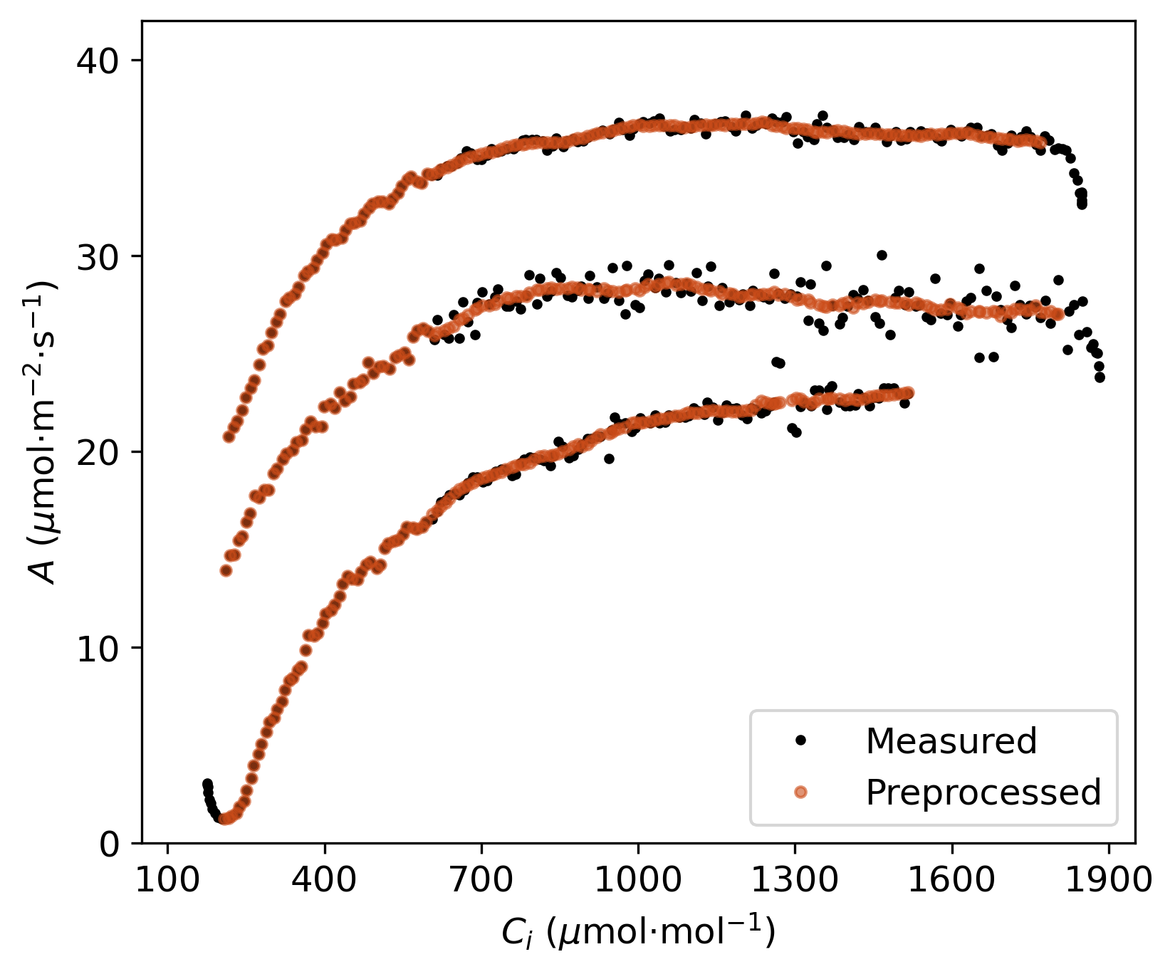
Figure 1: Example illustration of optional automated pre-processing of measured $A/C_{i}$ curves to smooth and remove artifacts at the beginning and end of the curves. The black and red points represent measured raw and pre-processed sample points, respectively.

2.5.2 PyTorch parameter optimizer (Adam)

As a popular deep learning architecture, PyTorch (Paszke et al., 2019) provides many important features that are beneficial for fitting photosynthesis curves. It can automatically compute gradients, which refers to the derivative of the loss function with respect to the parameters, of a customized model through a process called automatic differentiation. The loss function (i.e., error function to be minimized during fitting) can also be flexibly customized. Furthermore, some built-in activation functions can help constrain the range of FvCB parameters. For example, the sigmoid function $\sigma(x)=\frac{1}{1+e^{-x}}$ can ensure $\alpha_{g}$ remains within the range of 0 to 1.

The Adaptive Moment Estimation (Adam) optimizer (Kingma and Ba, 2014) was the chosen algorithm for fitting the FvCB model bases on photosythesis response curves. Although PyTorch provides other optimizers such as stochastic gradient descent (SGD), these require more tuning of hyperparameters and are more suitable for conventional machine learning models. Adam uses first-order gradient-based optimization of stochastic objective functions, based on adaptive estimates of lower-order moments. Given an initial guess for a model parameter $k$ (e.g., $V_{cmax25}$), the value is updated iteratively according to:

$$k_{t}=k_{t-1}-l\frac{\hat{m}_{t}}{\sqrt{\hat{v}_{t}}+\epsilon},$$ (11)

where $t$ is the updating iteration, $l$ is the learning rate which determines how aggressively the parameter estimate is updated on each iteration (the default is set to 0.08 in PhoTorch), $\hat{m}_{t}$ represents the biased first moment estimate, which determines the direction of optimization and is calculated as exponential moving averages of the gradients, $\hat{v}_{t}$ denotes the biased second raw moment estimate, which scales down the step size in regions where gradients might cause instability and is calculated as the squared gradients, $\epsilon$ is a hyperparameter which is set to $10^{-8}$. Adam can automatically adjust the learning rate $l$ for each FvCB parameter individually based on estimates of the first and second moments of the gradients. This feature makes Adam very effective in FvCB model fitting, as the parameters of the FvCB model greatly vary in terms of their sensitivity, units, and magnitude. Additionally, Adam requires little tuning of hyperparameters and has high optimization efficiency. The default values of two hyperparameters (learning rate 0.08 and maximum iteration 20,000) work for most $A/C_{i}$ fitting cases.

2.5.3 Loss function

The loss function is the equation to be minimized by the optimizer, and quantifies the level of agreement between the measured photosynthesis data points and the FvCB model prediction given the current parameter set. The design of the loss function is crucial for fitting the FvCB model in order to obtain a reliable and accurate fit for arbitrary input data sets. The basic loss function is the mean squared error ($\mathrm{MSE}$) between the measured $A_{i}$ and predicted $\hat{A_{i}}$ net photosynthesis rates for a given parameter set:

$$\mathrm{MSE}=\frac{1}{n}\sum\limits_{k=1}^{n}(A_{k}-\hat{A}_{k})^{2},$$ (12)

where $n$ is the total number of measured data points.

Equation 12 forms the basis of the loss function, but additional penalty terms are added to constrain the model fit in order to increase robustness. Penalty terms are essentially additional errors added to the loss to enforce specific properties in the output curves (e.g., parameter constraints). With increasing $C_{i}$ we assume that the assimilation will progress from being Rubisco limited, to be being limited by RuBP regeneration, and then finally to being limited by triose phosphate utilization. We assume all response curves contain Rubisco, RuBP, and TPU limitation states, and the order of these three states is fixed. According to Eq. 2, 3 and 6, as long as leaf temperature and incident light remain nearly constant (though some fluctuation may exist), curves of the Rubisco-limited assimilation rate $A_{c}(C_{i})$ and the RuBP-limited assimilation rate $A_{j}(C_{i})$ remain nearly monotonically increasing, and the curve of the TPU-limited assimilation rate $A_{p}(C_{i})$ remains nearly constant ($\alpha_{g}=0$) or nearly monotonically decreasing ($\alpha_{g}>0$). Thus, the intersection point between $A_{c}(C_{i})$ and $A_{j}(C_{i})$ should always be lower than the point on $A_{p}(C_{i})$ with the same $C_{i}$, which can be expressed as:

$$C_{i,jc}=\arg\min_{k}|A_{j}(C_{i,k})-A_{c}(C_{i,k})|$$ (13)

where $A_{c}$ and $A_{j}$ curves are closest to each other at $C_{i,jc}$, and $|\cdot|$ denotes the absolute values. Then, the penalty can be given as:

$$\text{Penalty}_{cj>p}=\max[0,\quad\max[A_{j}(C_{i,jc}),A_{c}(C_{i,jc})]-A_{p}(C_{i,jc})].$$ (14)

The above penalty targets the closest points between the curves rather than the actual curve intersection points. The reason is that the $A/C_{i}$ curves are based on discrete data, so in most cases an exact intersection point does not exist. Therefore, penalties that force $A_{c}(C_{i})$ and $A_{j}(C_{i})$ to intersect each other should be added:

$$\text{Penalty}_{c>j}=\max\left[\beta-\sum\max\left[A_{c}(C_{i})-A_{j}(C_{i}),\quad 0\right],\quad 0\right],$$ (15)

$$\text{Penalty}_{c<j}=\max\left[\beta-\sum\max\left[A_{j}(C_{i})-A_{c}(C_{i}),\quad 0\right],\quad 0\right],$$ (16)

where $\beta$ is a constant specified by the user (default is 8). The $\text{Penalty}_{c>j}$ and $\text{Penalty}_{c<j}$ terms penalize the situation where $A_{c}(C_{i})$ is supposed to be greater than $A_{j}(C_{i})$ if the sum less than $\beta$ and where $A_{j}(C_{i})$ is supposed to be greater than $A_{c}(C_{i})$ if the sum less than $\beta$, respectively. In other words, these penalties are supposed to be zero only if $A_{c}(C_{i})$ and $A_{j}(C_{i})$ intersect with each other sufficiently.

An additional constraint is added to ensure that a transition to TPU limitation occurs within the measured response curve, otherwise the gradient with respect to $TPU_{25}$ will vanish. Thus, a penalty is added when the last point (i.e., highest measured $C_{i}$) of $A_{p}$ is greater than that of $A_{j}$:

$$\text{Penalty}_{j<p}=\max[0,A_{p}(C_{i,last})]-A_{j}(C_{i,last})].$$ (17)

This penalty forces $A_{p}(C_{i})$ to move down until its last point is lower than that of $A_{j}(C_{i})$. As $A_{j}(C_{i})$ is nearly monotonically increasing and $A_{p}(C_{i})$ is flat or monotonically decreasing, the penalty has little effect on the final reconstruction even if the $A/C_{i}$ curve has no TPU limitation stage, ensuring that the parameter ($TPU$ or $TPU_{25}$) always has gradient. After fitting, the difference $A_{p}(C_{i,last})-A_{j}(C_{i,last})$ can be used to identify whether the target $A/C_{i}$ curve has a TPU limitation stage. This penalty can also be turned off if the user is fitting the light response curve.

As previously reported, $V_{cmax}$ and $J_{max}$ are highly correlated (Wullschleger, 1993; Medlyn et al., 2002; Fan et al., 2011). Thus, an optional penalty of a low correlation coefficient $r$ between $V_{cmax}$ and $J_{max}$ was added to prevent the occurrence of anomalous values in some cases. Users can choose to turn this penalty on or off, and this penalty is only used when at least 7 curves are being fitted simultaneously. The correlation coefficient $r$ is defined as:

$$r(x,y)=\frac{\sum\limits_{i}(x_{i}-\overline{x})(y_{i}-\overline{y})}{\sqrt{\sum\limits_{i}(x_{i}-\overline{x})^{2}\sum\limits_{i}(y_{i}-\overline{y})^{2}}},$$ (18)

where $\overline{x}$ and $\overline{y}$ are the mean values of all data points in $x$ and and $y$ respectively. Then the penalty can be defined as:

$$\text{Penalty}_{r}=\max[0,0.7-r(V_{cmax},J_{max})].$$ (19)

According to Eq. 19, when $r(V_{cmax},J_{max})$ is less than 0.7, $\text{Penalty}_{r}$ will be positive; otherwise, it is 0, which means no penalty. As illustrated by previous work (e.g., Walker et al., 2014), a perfect correlation between $V_{cmax}$ and $J_{max}$ is not expected. Accordingly, this penalty is not particularly strict and is only meant to minimize the presence of outlier values.

For small non-negative parameters such $\Delta{H_{a}}$ or $R_{d25}$, penalties are also added to prevent negative values:

$$\text{Penalty}_{k<0}=\max[0,-k].$$ (20)

The overall loss to be optimized is the sum of above mentioned $MSE$ (Eq. 12 and penalties (Eqs. 14, 15, 16, 17, 19, 20).

2.6 Field gas exchange data for method evaluation

Field gas exchange data was collected across variable CO₂, light, and temperature regimes in order to evaluate the proposed model calibration methodology. Measurements were taken within a common/tepary bean (Phaseolus vulgaris and Phaseolus acutifolius) and cowpea (Vigna unguiculata) breeding trial using an LI-6800 Portable Photosynthesis System (LI-COR Biosciences, Lincoln, Nebraska, USA) from June to August, 2022. The field was located in Davis, CA, United States. The breeding trials consisted of diversity panels of cowpea and bean genotypes, from which 5 plots of each were selected that represented high genetic diversity in terms of flowering time, yield, and growth structure, which also carried many traits relevant to abiotic and biotic stress resistance. Table 4 illustrates the details of the collected gas exchange data, and their pedigrees are listed in Table 1 of Appendix A. Measurements were made on fully sunlit and fully expanded, healthy leaves between the hours of 9:00 and 12:00. $A/C_{i}$ curves were run in non-steady-state mode using the LI-6800’s Dynamic Assimilation Technique (DAT). Light response curves were obtained through separate response runs based on steady-state measurements at each light level. For the $A/C_{i}$ curves, the reference relative humidity was set to 50%, the incident light flux was set to 2000 $\mu$mol/m²/s, the CO₂ ramp rate was 300 $\mu$mol/mol/min for the DAT, the fan speed was 10,000 rpm, and the starting and ending CO₂ concentration setpoints were 200 and 1800 $\mu$mol/mol, respectively. The leaf temperature setpoint was varied to be approximately 25, 30, and 40°C, and unique leaves were sampled for each $A/C_{i}$ curve at the different temperatures. On each sampling day, all genotypes were sampled at all temperatures, with each curve being on a different leaf, and all measurements across multiple sampling days for a given genotype were aggregated to extract temperature parameters. All genotypes were sampled at a given temperature before moving on to the next higher temperature. For the light response curve, relative humidity was set to 60%, leaf temperature was fixed to 25°C, fan speed was 3,000 rpm, incident PPFD values were set to 0, 150, 400, 800, 1200, and 2000 $\mu$mol/m²/s.

Oak (Quercus coccinea Münchh) $A/C_{i}$ curves measured in steady-state from an openly accessible dataset (Burnett et al., 2021) were also used to evaluate PhoTorch’s fitting ability. It contains 6 $A/C_{i}$ curves measured using an LI-6800 and 35 using a LICOR LI-6400. Incident PPFD values were set to 1500 $\mu$mol/m²/s, and leaf temperature ranged from 22 to 28°C. The dataset can be downloaded from Ecological Spectral Information System (Wagner et al., 2018).

Table 4: Overview of cowpea and bean gas exchange datasets used for method evaluation.

Species	Line ID	Number of curves	Number of total data points
Cowpea	aMAGIC015	11	2027
Cowpea	MAGIC179	11	1857
Cowpea	MAGIC043	11	1836
Cowpea	MAGIC043	b1	6
Cowpea	MAGIC143	11	1857
Cowpea	MAGIC184	11	1833
Tepary Bean	cTARS-Tep 23	13	2125
Interspecific Common/Tepary Bean	dNE-80-21-46	11	1902
Interspecific Common/Tepary Bean	NE-80-21-2	12	2054
Interspecific Common/Tepary Bean	NE-80-21-233	12	2028
Interspecific Common/Tepary Bean	eINB 841	12	2045

^a: These “MAGICXXX” genotypes are from the cowpea MAGIC population derived from eight parents (Huynh et al., 2018).

^b: Steady-state light response curve.

^c: TARS-Tep 23 is a tepary line released by Porch et al. (2022).

^d: The three “NE-80-21-XX” common bean/tepary bean interspecific lines with prefixes of NE are common bean/tepary bean interspecific lines that were developed from crosses described in Barrera et al. (2022).

^e: INB 841 is a common bean/tepary bean interspecific line that was developed from five cycles of congruity backcrossing of tepary with ICA Pijao (Mejía-Jiménez et al., 1994).

2.7 Evaluation of method performance

The coefficient of determination $R^{2}$ and the root mean square error ($\mathrm{RMSE}$) were used as evaluation metrics to quantify the goodness of model fit. The $R^{2}$ for each curve fit is given as:

$$R^{2}=1-\frac{\sum\limits_{i}(A_{i}-\hat{A}_{i})^{2}}{\sum\limits_{i}(A_{i}-\bar{A})^{2}},$$ (21)

where $\bar{A}$ is the mean value of all data points in $A$, and $\hat{A}$ is the fitted $A$. The $\mathrm{RMSE}$ is simply the square root of $\mathrm{MSE}$ in Eq. 12:

$$\mathrm{RMSE}=\sqrt{\frac{1}{n}\sum\limits_{i}(A_{i}-\hat{A}_{i})^{2}}.$$ (22)

For curves in one genotype, the model will fit their own four main parameters $V_{cmax25}$, $J_{max25}$, $\mathrm{TPU_{25}}$, and $R_{d25}$. For the light and temperature parameters, all curves for a given genotype will share the same set of parameters.

The plantecophys package (Duursma, 2015) was used as a benchmark for comparison. As plantecophys does not have the option for temperature response fitting, the temperature response option of PhoTorch was set to 0 when used for these comparisons. $\alpha$, $\Delta{H_{a,V_{cmax}}}$ and $\Delta{H_{a,J_{max}}}$ of PhoTorch were set to 0.24, 58.5 and 29.68, respectively, for comparison, in accordance with default settings of plantecophys. No pre-processing procedure was applied to the original data. It should be noted that the error metric output from plantecophys is actually the ‘root sum squared error’, although they call it ‘root mean squared error’ ($\mathrm{RMSE}$). Therefore, plantecophys fitting results were used to calculate $RMSE$ as defined in Eq. 22 for consistency in comparison with PhoTorch.

PhoTorch was also tested by fitting to synthetic $A/C_{i}$ curves generated using the FvCB model, with known parameters obtained by randomly scaling those extracted by PhoTorch with a positive $R_{d}$ constraint (PhoTorch ($\pm R_{d}$)) in Table 5 by 90% to 110%. Different levels of Gaussian noise were also added to the synthetic $A/C_{i}$ curves. The number of added Gaussian noise data points is the same as the number of data points in a target $A/C_{i}$ curve. The noise data points are independently sampled with a mean of zero and a varying standard deviation using the function torch.randn().

3 Results

3.1 Non-steady-state $A/C_{i}$ curves at variable temperatures

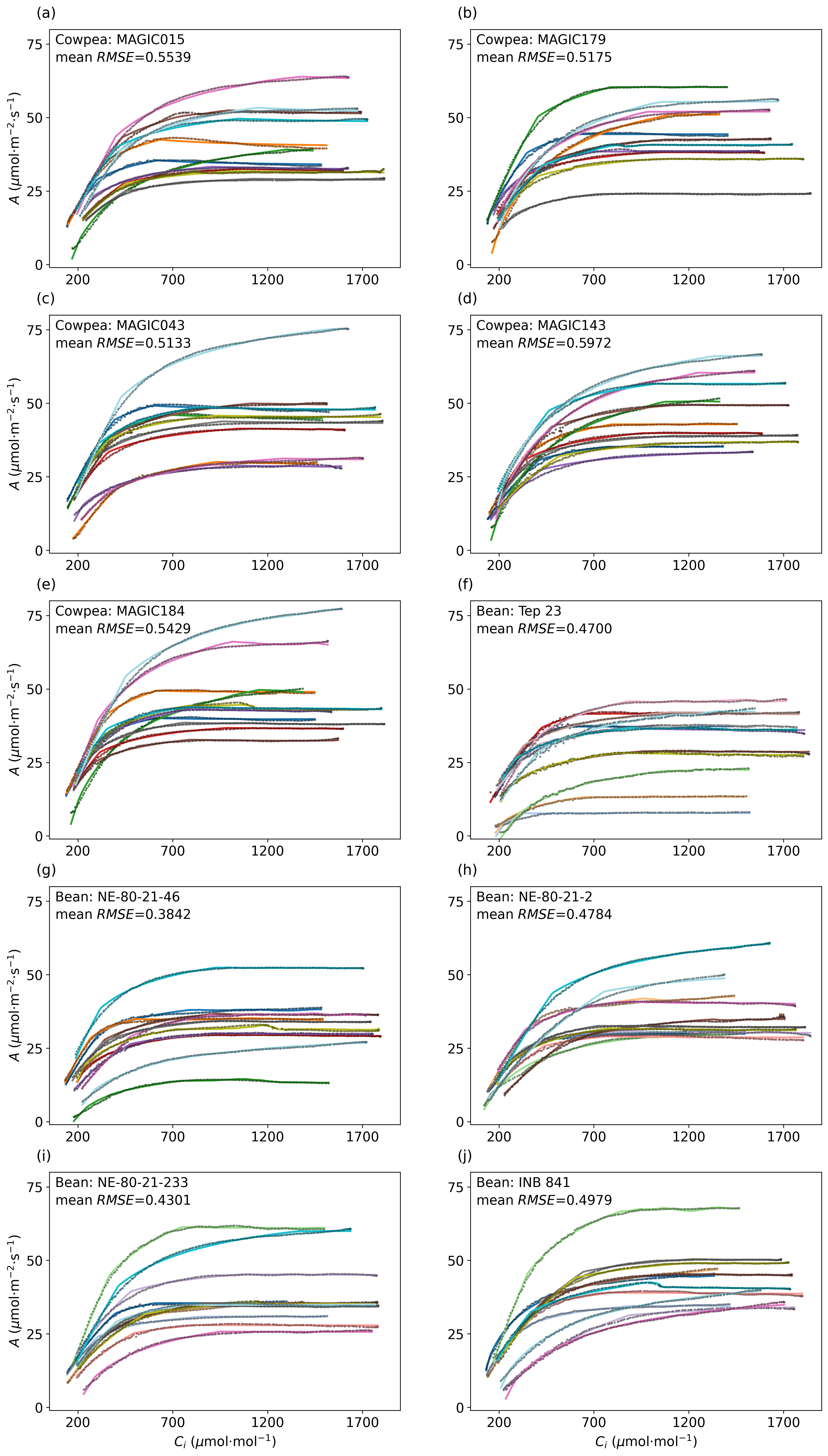
Figure 7: Results of $A/C_{i}$ fitting based on bean and cowpea field gas exchange data, excluding the light response curve. The dotted points are measured $A/C_{i}$ values and solid curves are $A/C_{i}$ curves produced by the fitted FvCB model. The learning rate and maximum iterations were set to 0.08 and 20,000 for all fittings.

Figure 2 shows the result of $A/C_{i}$ curve fitting for the bean and cowpea datasets at constant light and based on an Arrhenius temperature response (light response type of 0 and temperature response type of 1). The mean $\mathrm{RMSE}$ and $R^{2}$ are 0.4973 ($\mu$mol/m²/s) and 0.9917, respectively, using the same optimizer settings across all curves, indicating a good fit. Figure 7 presents more detailed fitting results. The mean $\mathrm{RMSE}$ for fittings across all curves is within the range of 0.38-0.6. The resulting fit was nearly perfect with all $R^{2}$ above 0.99 except the ‘Tep 23’ curve, which still has a high $R^{2}$ of 0.972 (Fig. 7). These results demonstrate the robust performance of PhoTorch.

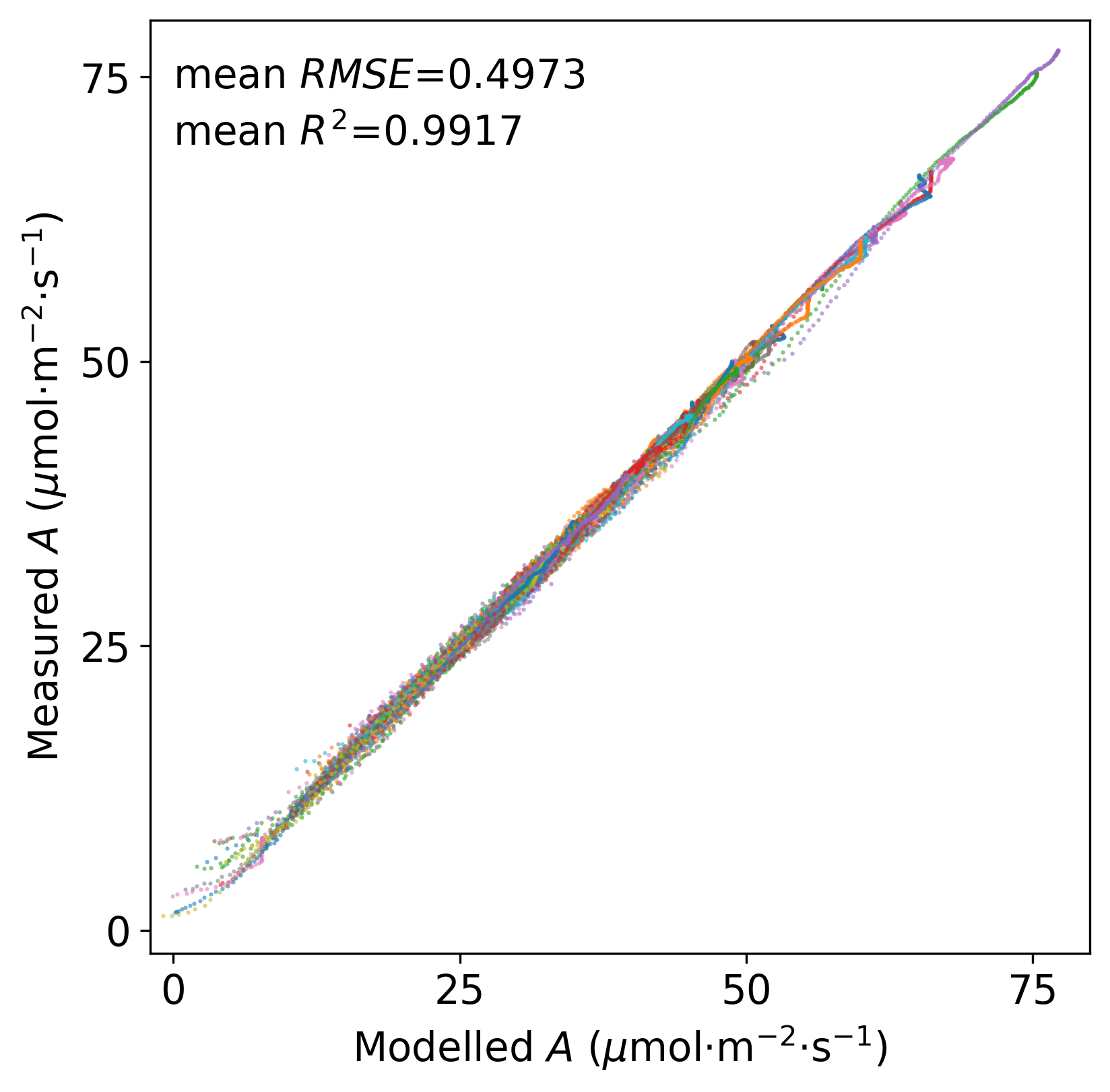
Figure 2: Results of $A/C_{i}$ fitting based on bean and cowpea field gas exchange data, excluding the light response curve. The horizontal and vertical coordinate of each point respectively corresponds to the modelled and measured $A$ values at each $C_{i}$ value. The learning rate and maximum iterations were set to 0.08 and 20,000 for all fittings.

Resulting fitted parameters showed an approximately linear relationship between $V_{cmax25}$ and $J_{max25}$ (Fig. 3), which is in agreement with prior observations (Wullschleger, 1993; Medlyn et al., 2002; Walker et al., 2014; Kumarathunge et al., 2019b) and supported by theoretical arguments of optimal allocation of photosynthetic capacity (Quebbeman and Ramirez, 2016). For this dataset the correlation between $V_{cmax25}$ and $J_{max25}$ was $r^{2}=0.53$ for both cowpea and bean, which is higher than the optional $r$ penalty (penalized when $r^{2}<0.49$). For cowpea the ratio $J_{max25}$:$V_{cmax25}$ was 2.02, and was 2.03 for bean. Wullschleger (1993) reported an average ratio of 2.05 across a set of annual species, and Medlyn et al. (2002) reported an average of 1.67 across a range of plant functional types, including a ratio of 2.4 in soybean. Their previously reported ratios demonstrate that the ratio $J_{max25}$:$V_{cmax25}$ we extracted is reasonable.

The fitted $\Delta{H_{a}}$ parameters displayed in Fig. 4 are indicative of the response of net photosynthesis to temperature, and could be used as a breeding trait for selecting genotypes with high or low sensitivity to temperature. The temperature responses of Rubisco-limited and electron transport-limited carboxylation rates, as represented by $\Delta{H_{a,V_{cmax}}}$ and $\Delta{H_{a,J_{max}}}$, appear positively correlated, with clear separation between cowpea and bean species (Fig. 4). Bean exhibits higher photosynthetic temperature optima than cowpea, however, the mean of the maximum $A$ of each curve of bean and cowpea are 37.41 and 45.17 $\mu$mol/m²/s, respectively, suggesting a trade-off between maximum photosynthetic capacity and heat tolerance. Our fitting results suggest that the temperature response of the triose-phosphate limited pathway, $\Delta{H_{a,\mathrm{TPU}}}$, however, is negatively correlated to that of the above two pathways, which is consistent with the findings of Kumarathunge et al. (2019a).

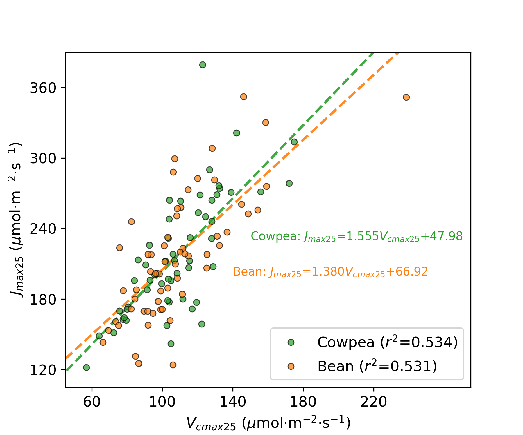
Figure 3: Fitted $V_{cmax25}$ versus $J_{max25}$ for each $A/C_{i}$ curve in the cowpea and bean datasets. Dashed lines give the best linear fit for each species.

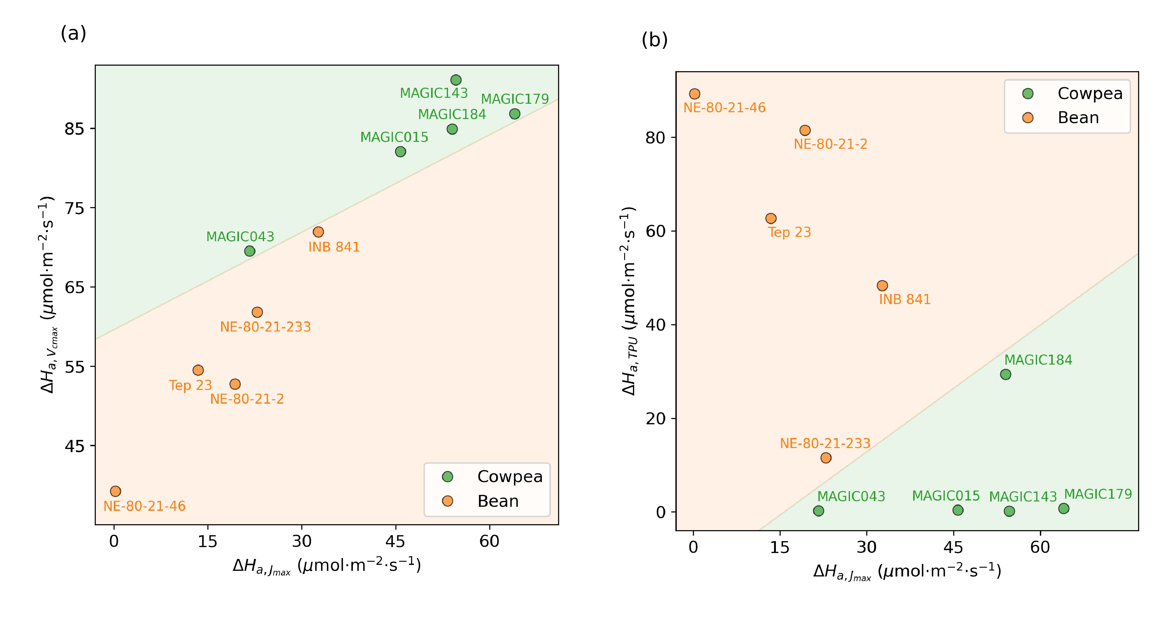
Figure 4: Correlation between temperature response parameters for each genotype in the bean and cowpea datasets. (a) Fitted $\Delta{H_{a,J_{max}}}$ versus fitted $\Delta{H_{a,V_{cmax}}}$. (b) Fitted $\Delta{H_{a,J_{max}}}$ versus fitted $\Delta{H_{a,\mathrm{TPU}}}$. Colored zones delineate bean and cowpea genotypes.

3.2 Fitting non-steady-state $A/C_{i}$ curves with steady-state light response

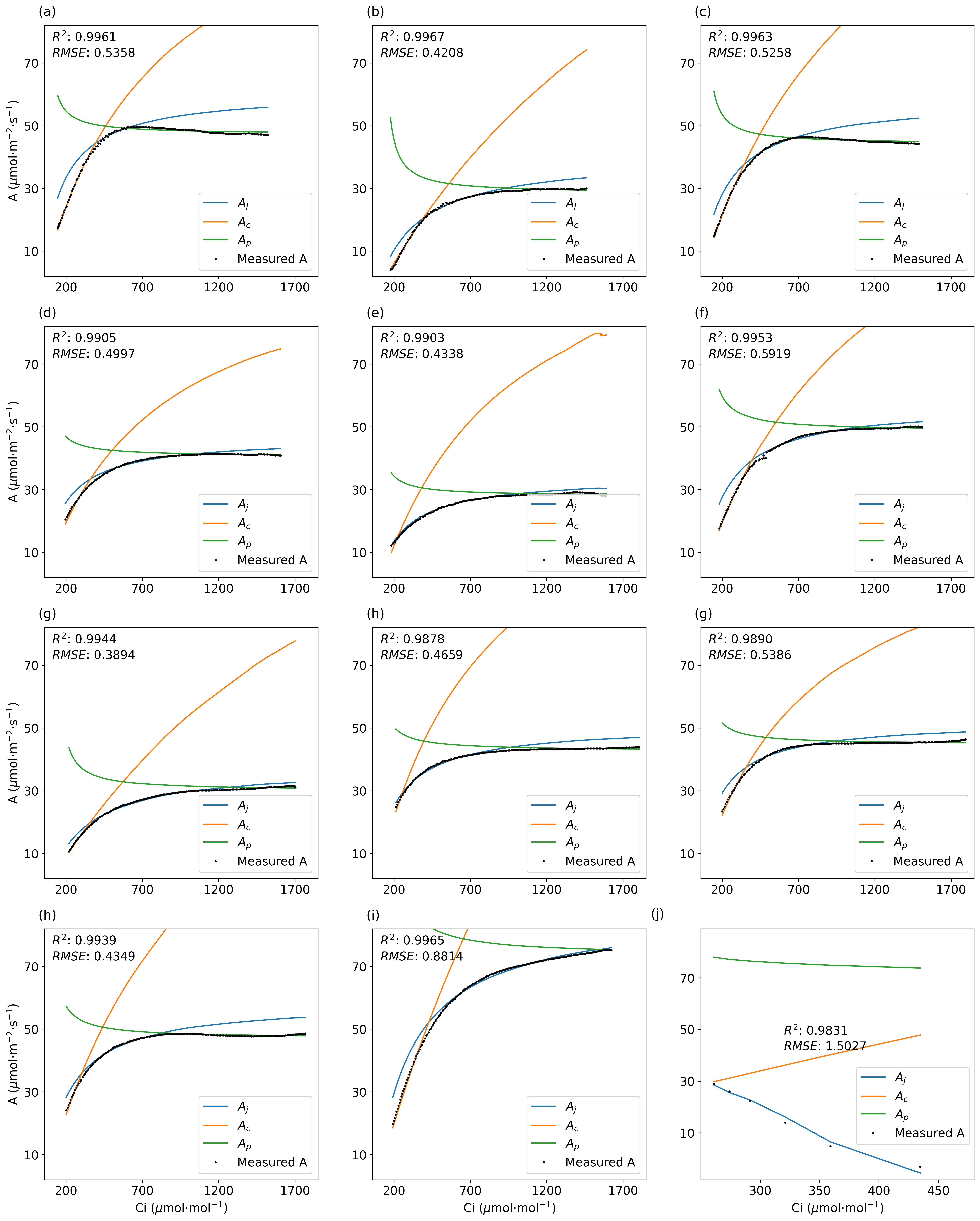
Figure 8: Fitted $A_{c}$, $A_{j}$, and $A_{p}$ curves, and measured $A$ values (black dot points) for cowpea of genotype MAGIC043. Selected light response type is 1 (learnable parameter is $\alpha$ in Eq. 4). The learning rate and maximum iteration were set to 0.08 and 20,000 for all fittings. Each plot has its own set of main four parameters, but all plots share the same set of temperature and light response parameters.

The present optimizer can also simultaneously fit $A/C_{i}$ curves and light response curves ($A/Q$). Figures 8 and 9 show fitted $A_{c}$, $A_{j}$, and $A_{p}$ and measured $A$ including the light response curves (Fig. 8j and 9j). The $A_{p}$ in both light response plot in Fig. 8 and 9 are not updated, which prevents failure of fitting. All fitting results using both light response types 1 and 2 had very high goodness of fit and appear visually reasonable. The goodness of fit for the light response curve in Fig. 9j (non-rectangular hyperbola) is better than that of Fig. 8j (rectangular hyperbola). This result is reasonable since the light response type 2 has more degrees of freedom due to its two parameters, $\alpha$ and $\theta$, whereas light response type 1 only has one, $\alpha$. The $A/Q$ curves demonstrate clearer fitting results for two light response cases (Fig. 5). These results indicate that the present optimizer can fit $A/C_{i}$ curves and light response curves ($A/Q$) simultaneously with high accuracy.

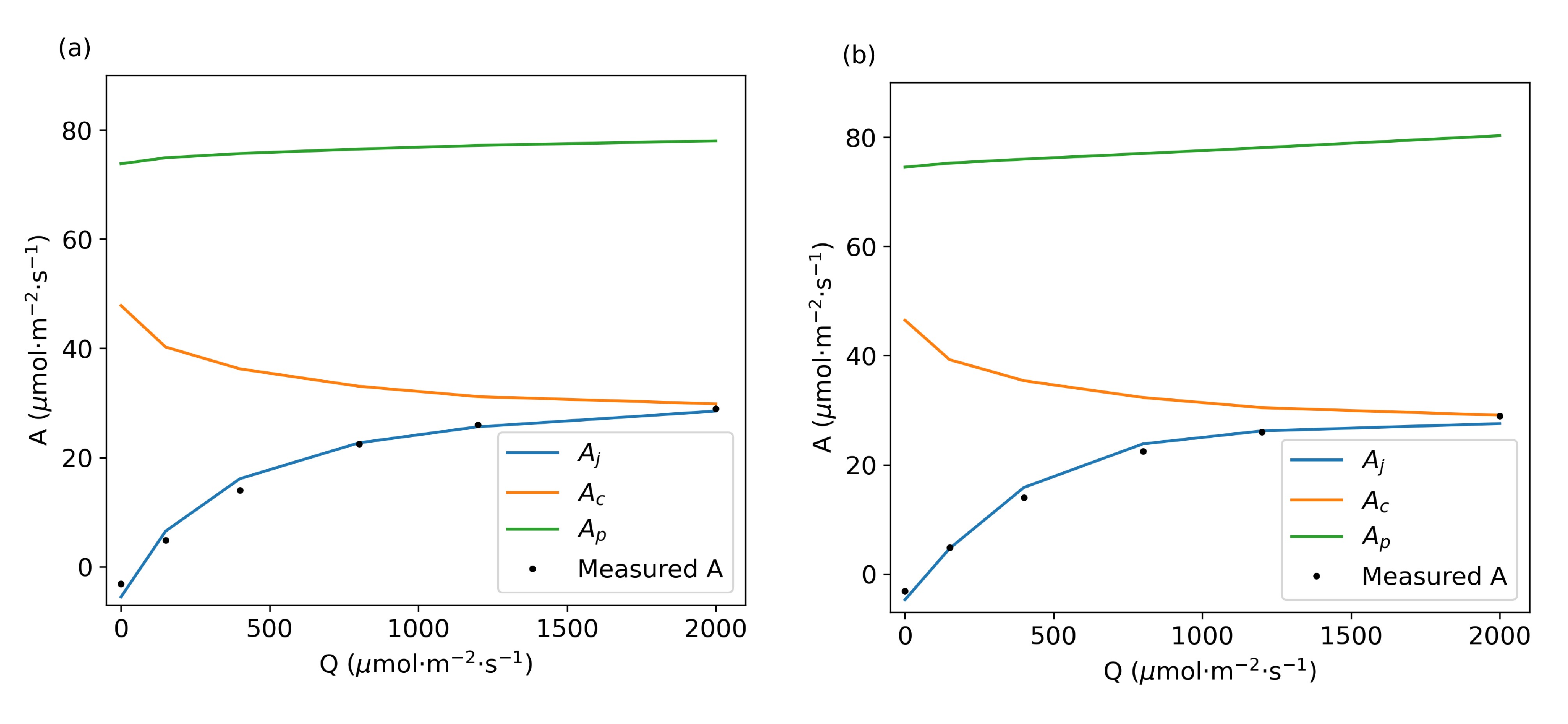
Figure 5: Fitted $A_{c}/Q$, $A_{j}/Q$, and $A_{p}/Q$ curves, and measured $A/Q$ (black dot points) for light response type 1 (a) and 2(b). Curves in (a) and (b) are the same as curves from Fig. 8j and 9j, respectively.

3.3 Comparison of non-steady-state $A/C_{i}$ fitting with plantecophys

As it is one of the most popular $C_{3}$ plant $A/C_{i}$ curve fitting packages, plantecophys was used as a benchmark against which PhoTorch could be compared. Table 5 shows the $\mathrm{RMSE}$ results obtained using plantecophys and PhoTorch with and without the positive $R_{d}$ constraint. For the $A/C_{i}$ curves considered in this test, the overall goodness of fit between plantecophys and PhoTorch was similar. In some cases, plantecophys was able to achieve an artificially good fit (mean $\mathrm{RMSE}=0.4639$ $\mu$mol/m²/s) by allowing $R_{d}$ to be negative. However, if the positive constraint was removed in PhoTorch, the mean $\mathrm{RMSE}$ (0.4556) for PhoTorch was lower than plantecophys. These tests are limited by the fact that plantecophys cannot simultaneously fit light and temperature response, so it was not possible to benchmark these more complicated fitting cases.

A 12th Gen Intel Core i9-12950HX CPU was used to run all curve fits in Table 5. Results illustrate that PhoTorch was more than four times faster than plantecophys in performing the model fitting, which could be significant if processing a large amount of unsteady $A/C_{i}$ curves that contain hundreds of data points each.

Table 5: $\mathrm{RMSE}$ results obtained by plantecophys and PhoTorch for fitting $A/C_{i}$ curves of cowpea MAGIC043. $\mathrm{RMSE}$ values have units of $\mu$mol/m²/s.

aSample ID	bplantecophys	cPhoTorch (+$R_{d}$)	dPhoTorch ($\pm R_{d}$)
5	0.7519	0.5746	0.4705
7	0.4497	0.5134	0.5443
8	0.6280	0.5234	0.4221
41	0.3274	0.5130	0.3368
43	0.4221	0.4298	0.4341
48	0.4954	0.5318	0.5436
51	0.3617	0.4371	0.3929
102	0.2737	0.4027	0.3118
105	0.3632	0.5535	0.4624
108	0.3478	0.4383	0.3761
114	0.6821	0.8783	0.7170
Mean	0.4639	0.5269	0.4556
Fitting time	287s	64s	64s

^a: Sample IDs are provided by the original dataset.

^b: The “fitacis” funtion was used and its option “fitTPU” was set to “True”, “EdVC” ($\Delta{H_{d,V_{cmax}}}$) was set to 0,“EdVJ” ($\Delta{H_{d,J_{max}}}$) was set to 0,“Tcorrect” was set to “FALSE”; other settings were set to default. It should be noted that $R_{d}$ does not have positive constraint in plantecophys.

^c: The temperature and light response types were set to 0, and $K_{c25}$, $K_{o25}$, and $\Gamma_{25}^{*}$ were not fitted. $R_{d}$ has positive constraint. The learning rate and maximum iteration were set to 0.08 and 20,000, respectively.

^d: $R_{d}$ did not have positive constraint, other settings were same with ^c.

Figure 6 displays the fitted $V_{cmax}$, $J_{max}$, $TPU$, and $R_{d}$ parameters for all samples of cowpea MAGIC043 using plantecophys, PhoTorch with a positive $R_{d}$ constraint, and PhoTorch without a $R_{d}$ constraint. Generally, PhoTorch without a positive $R_{d}$ constraint produced parameter estimates similar to those fitted by plantecophys. However, compared to the parameters fitted by PhoTorch with a positive $R_{d}$ constraint, $V_{cmax}$, $J_{max}$, and $TPU$ were underestimated. The parameters for curve 43 (Table 5) show the most significant difference between plantecophys and the two PhoTorch fittings. Although the “true” parameters are unknown, the $V_{cmax}$, $J_{max}$, and $TPU$ fitted by plantecophys are the lowest among all, which may indicate that the plantecophys fitting result is not reliable for this curve.

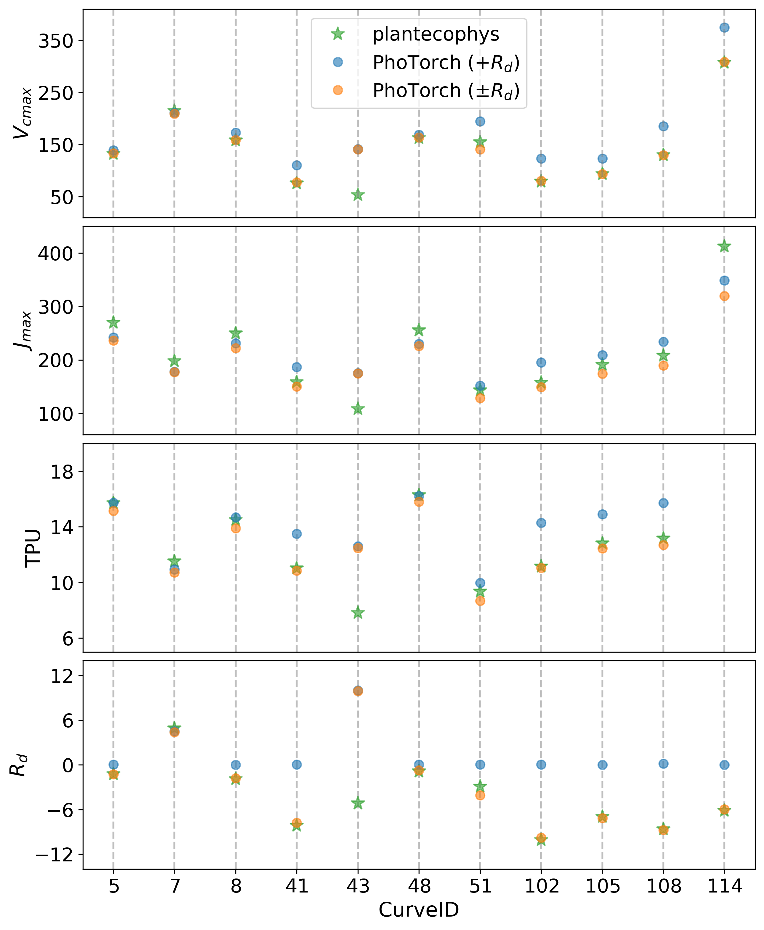
Figure 6: Fitted $V_{cmax}$, $J_{max}$, $TPU$, and $R_{d}$ parameters for all samples of cowpea MAGIC043 using plantecophys (green star), PhoTorch with a positive $R_{d}$ constraint (blue circle), and PhoTorch without an $R_{d}$ constraint (orange circle).

3.4 Fitting synthetic $A/C_{i}$ curves

Table 6 presents the $\mathrm{RMSE}$ results of parameter estimation from synthetic $A/C_{i}$ curves using PhoTorch. As expected, the fitted parameters are closer to the known parameters when the noise level is lower. Even at high noise levels, the fitted parameters remain reasonable, demonstrating the robustness of PhoTorch. It is worth noting that a standard deviation of 1.5 represents a significant amount of noise, with 95% of the data points deviating between -3 and 3 $\mu$mol/m²/s around the original curve. The noise especially impacts the Rubisco-limited state ($V_{cmax}$), as the $A$ values in this state are much lower than than in other states, and thus the magnitude of the noise is closer to the magnitude of $A$ itself. This explains why the fitting results for $V_{cmax}$ have the highest $\mathrm{RMSE}$. When using the plantecophys to fit the synthetic $A/C_{i}$ curve with a 1.5 standard deviation noise, the results of $J_{max}$ ($>$40) and $R_{d}$ ($>$1) are not satisfactory. The main reason is that the plantecophys lacks a non-negative constraint for $R_{d}$.

Table 6: $\mathrm{RMSE}$ results of fitting synthetic $A/C_{i}$ curves with various standard deviations of Gaussian noise. All values have units of $\mu$mol/m²/s.

Standard deviation of Gaussian noise	$V_{cmax}$ $\mathrm{RMSE}$ (mean: 181.38 $\mu$mol/m2/s)	$J_{max}$ $\mathrm{RMSE}$ (mean: 216.02 $\mu$mol/m2/s)	$R_{d}$ $\mathrm{RMSE}$ (mean: 1.34 $\mu$mol/m2/s)
1.5	6.6208	6.3433	0.6874
1	3.8251	3.2686	0.6657
0.5	2.1196	1.2249	0.2831
0.2	1.4774	1.3708	0.2691
0	0.5329	0.3463	0.0717

Note: Since $\mathrm{TPU}$ limitation states did not appear in some curves, the $\mathrm{TPU}$ fitting results were not compared. No pre-processing procedure was applied to the noisy curves.

3.5 Fitting all available parameters for both steady-state and non-steady-state $A/C_{i}$ curves

Table 7 presents fitting results for the oak tree, cowpea, and bean datasets, where all possible parameters were fitted except for $g_{m}$ and light response parameters (see Table 7). The cowpea and bean curves consist of all $A/C_{i}$ curves presented in Table 4 except the light response curve. Each curve has its own fitted $V_{cmax25}$, $J_{max25}$, $\mathrm{TPU_{25}}$, and $R_{d25}$ value, while all other parameters listed in Table 7 are shared within the same species. Low $\mathrm{RMSE}$ ($<$0.5 $\mu$mol/m²/s) and high $R^{2}$ ($>$0.98) values were obtained for both steady-state and non-steady-state $A/C_{i}$ curves, demonstrating the flexibility and generality of PhoTorch when fitting a large number of parameters. While the cowpea and bean datasets contain a wide range of temperature conditions that exceed the photosynthetic temperature optimum, it should be noted that the temperature response parameters for oak may be unreliable due to the small measured temperature range in the dataset (22-28°C).

Table 7: Fitted parameters for datasets from 3 species, containing both steady-state and non-steady-state $A/C_{i}$ curves. All possible parameters were fitted except for the mesophyll conductance $g_{m}$ and the light response parameters (the oak dataset lacked this data). The fitting produced a unique $V_{cmax25}$, $J_{max25}$, $\mathrm{TPU_{25}}$, and $R_{d25}$ for each $A/C_{i}$ curve (not reported), whereas each value reported in the table is the value fitted across all curves in each species. Error metrics were calculated for the fit to each curve, and the reported value is the mean value across all curves.

Parameter	Oak	Cowpea	Bean
Mean $\mathrm{RMSE}$ ($\mu$mol/m2/s)	0.4919	0.4784	0.4649
Mean $R^{2}$	0.9884	0.9950	0.9873
$K_{c25}$	450.7	322.8	364.9
$K_{o25}$	220.9	360.8	320.2
$\Gamma_{25}^{*}$	42.95	48.40	43.44
$\Delta{H_{a,V_{cmax}}}$	64.54	64.22	60.59
$\Delta{H_{a,J_{max}}}$	82.41	57.51	30.49
$\Delta{H_{a,\mathrm{TPU}}}$	47.48	15.71	48.50
$T_{opt,V_{cmax}}$	293.8	310.5	313.3
$T_{opt,J_{max}}$	298.5	311.2	312.6
$T_{opt,\mathrm{TPU}}$	301.0	302.2	313.3
$\alpha_{g}$	1.4574	0.1280	0.0546
Instrument	LI-6400 & LI-6800	LI-6800	LI-6800
State of response	Steady-state	*Dynamic	Dynamic
Number of curves	41	55	60
Number of points	566	9410	10154

*: “Dynamic” refers to Dynamic Assimilation™ Technique feature of the LI-6800, which is a non-steady-state measurement.

4 Discussion

Novel FvCB model fitting software was developed based on optimizers within the PyTorch deep learning framework, which was demonstrated to be able to flexibly and efficiently fit to a range of leaf-level photosynthesis CO₂, light, and temperature response data without any ad hoc parameter tuning. The resulting set of fitted parameters quantifies photosynthetic response to these environmental factors, which can benefit plant ecophysiological research. For instance, Kumarathunge et al. (2019b) empirically found the ratio of $J_{max25}$ to $V_{cmax25}$ to be negatively correlated with the plant’s acclimation temperature as well as evolutionarily-adapted temperature. Theoretical arguments and empirical observations of Quebbeman and Ramirez (2016) suggest that $J_{max25}$:$V_{cmax25}$ should increase linearly with nitrogen content, decrease exponentially with maximum daily irradiance, and be able to vary on a monthly timescale. These findings highlight the importance of robust photosynthetic parameter estimation for understanding plant responses to varying environmental conditions, which the PhoTorch software can provide.

Leveraging of the PyTorch framework, originally developed for machine learning applications, facilitated robust parameter optimization with high computational efficiency, and the ability to enforce a number of constraints that ensure robustness in the presence of unusual or noisy gas exchange data. In addition, as the FvCB model was written entirely in PyTorch, it can be easily integrated with other AI models used in photosynthesis research. This feature is especially beneficial for expanding typical phenotyping studies focused on predicting photosynthesis traits from indirect measurements using machine learning models (Camino et al., 2022; Deng et al., 2024). These studies seek to predict FvCB parameters from sensing data such as leaf reflectance spectra or images, which relies on parameters fitted from ground truth $A/C_{i}$ curves, making the entire workflow a two-stage process (first fitting $A/C_{i}$ curves, then predicting the fitted parameters using sensing data). However, the present package allows for directly connecting the FvCB model with deep learning models, integrating them into a unified deep learning model. This enables the direct fitting of $A/C_{i}$ curves using sensing data, which could potentially improve the reliability of phenotyping models.

Declaration of Competing Interest

The authors declare that they have no known competing financial interests or personal relationships that could have appeared to influence the work reported in this paper.

Appendix Appendix A Pedigrees of common/tepary bean used

Table 1: Pedigree of bean and cowpea genotypes used for field data collection.

Line ID	Pedigree
NE-80-21-2	(VAP 1xG 40019)F1 X SEF 10/-001F1-001C-02C-MC-MC-02L-MSB
NE-80-21-46	((VAP 1xG 40019)F1 X SEF 10)F1 X SMC 214/-002F1-04C-MC-MC-01L-MSB
NE-80-21-233	(((((INB 834xG 40264)F1 X INB 834)F1 X INB 841)-003F1 X G 40036)F1 X ICTA LIGERO)F1 X SEF 10/-004F1-02C-MC-MC-01L-MSB
TARS-Tep 23	PI 502217-s x PI 440799
INB 841	INB108 x INB605
MAGIC015	[(CB27 x IT82E-18) x (IT89KD-288 x IT84S-2049)] x [(Suvita2 x IT00K-1263) x (IT84S-2246 x IT93K-503-1)]
MAGIC043	[(CB27 x IT82E-18) x (IT89KD-288 x IT84S-2049)] x [(Suvita2 x IT00K-1263) x (IT84S-2246 x IT93K-503-1)]
MAGIC143	[(CB27 x IT82E-18) x (IT89KD-288 x IT84S-2049)] x [(IT84S-2246 x IT93K-503-1) x (Suvita2 x IT00K-1263)]
MAGIC179	[(CB27 x IT82E-18) x (IT89KD-288 x IT84S-2049)] x [(Suvita2 x IT00K-1263) x (IT84S-2246 x IT93K-503-1)]
MAGIC184	[(CB27 x IT82E-18) x (IT89KD-288 x IT84S-2049)] x [(Suvita2 x IT00K-1263) x (IT84S-2246 x IT93K-503-1)]

Appendix Appendix B Fitting results supplementary figures

Figure 9: Fitted $A_{c}/C_{i}$, $A_{j}/C_{i}$, and $A_{p}/C_{i}$ curves, and measured $A/C_{i}$ values (black dot points) for cowpea of genotype MAGIC043. Selected light response type is 2 (learnable parameters are $\alpha$ and $\theta$ in Eq. 4). The learning rate and maximum iteration were set to 0.08 and 20,000 for all fittings.

References

- Barrera et al. (2022) Barrera, S., Berny Mier y Teran, J.C., Lobaton, J.D., Escobar, R., Gepts, P., Beebe, S., Urrea, C.A., 2022. Large genomic introgression blocks of Phaseolus parvifolius Freytag bean into the common bean enhance the crossability between tepary and common beans. Plant Direct 6, e470.
- Bellasio et al. (2016) Bellasio, C., Beerling, D.J., Griffiths, H., 2016. An Excel tool for deriving key photosynthetic parameters from combined gas exchange and chlorophyll fluorescence: theory and practice. Plant, Cell & Environment 39, 1180–1197.
- Bernacchi et al. (2001) Bernacchi, C., Singsaas, E., Pimentel, C., Portis Jr, A., Long, S.P., 2001. Improved temperature response functions for models of Rubisco-limited photosynthesis. Plant, Cell & Environment 24, 253–259.
- Burnett et al. (2019) Burnett, A.C., Davidson, K.J., Serbin, S.P., Rogers, A., 2019. The “one-point method” for estimating maximum carboxylation capacity of photosynthesis: A cautionary tale. Plant, Cell & Environment 42, 2472–2481.
- Burnett et al. (2021) Burnett, A.C., Serbin, S.P., Lamour, J., Anderson, J., Davidson, K.J., Yang, D., Rogers, A., 2021. Seasonal trends in photosynthesis and leaf traits in scarlet oak. Tree Physiology 41, 1413–1424.
- Busch et al. (2024) Busch, F.A., Ainsworth, E.A., Amtmann, A., Cavanagh, A.P., Driever, S.M., Ferguson, J.N., Kromdijk, J., Lawson, T., Leakey, A.D., Matthews, J.S., et al., 2024. A guide to photosynthetic gas exchange measurements: Fundamental principles, best practice and potential pitfalls. Plant, Cell & Environment .
- Camino et al. (2022) Camino, C., Araño, K., Berni, J.A., Dierkes, H., Trapero-Casas, J.L., León-Ropero, G., Montes-Borrego, M., Roman-Écija, M., Velasco-Amo, M.P., Landa, B.B., et al., 2022. Detecting Xylella fastidiosa in a machine learning framework using Vcmax and leaf biochemistry quantified with airborne hyperspectral imagery. Remote Sensing of Environment 282, 113281.
- De Kauwe et al. (2016) De Kauwe, M.G., Lin, Y.S., Wright, I.J., Medlyn, B.E., Crous, K.Y., Ellsworth, D.S., Maire, V., Prentice, I.C., Atkin, O.K., Rogers, A., et al., 2016. A test of the ‘one-point method’ for estimating maximum carboxylation capacity from field-measured, light-saturated photosynthesis. New Phytologist 210, 1130–1144.
- Deng et al. (2024) Deng, X., Zhang, Z., Hu, X., Li, J., Li, S., Su, C., Du, S., Shi, L., 2024. Estimation of photosynthetic parameters from hyperspectral images using optimal deep learning architecture. Computers and Electronics in Agriculture 216, 108540.
- Dubois et al. (2007) Dubois, J.J.B., Fiscus, E.L., Booker, F.L., Flowers, M.D., Reid, C.D., 2007. Optimizing the statistical estimation of the parameters of the Farquhar–von Caemmerer–Berry model of photosynthesis. New Phytologist 176, 402–414.
- Duursma (2015) Duursma, R.A., 2015. Plantecophys – an R package for analysing and modelling leaf gas exchange data. PloS One 10, e0143346.
- Ellsworth et al. (2015) Ellsworth, D.S., Crous, K.Y., Lambers, H., Cooke, J., 2015. Phosphorus recycling in photorespiration maintains high photosynthetic capacity in woody species. Plant, Cell & Environment 38, 1142–1156.
- Ethier and Livingston (2004) Ethier, G., Livingston, N., 2004. On the need to incorporate sensitivity to co2 transfer conductance into the Farquhar–von Caemmerer–Berry leaf photosynthesis model. Plant, Cell & Environment 27, 137–153.
- Fan et al. (2011) Fan, Y., Zhong, Z., Zhang, X., 2011. Determination of photosynthetic parameters Vcmax and Jmax for a C3 plant (spring hulless barley) at two altitudes on the Tibetan Plateau. Agricultural and Forest Meteorology 151, 1481–1487.
- Farquhar et al. (1980) Farquhar, G.D., von Caemmerer, S., Berry, J.A., 1980. A biochemical model of photosynthetic CO2 assimilation in leaves of C3 species. Planta 149, 78–90.
- Gu et al. (2010) Gu, L., Pallardy, S.G., Tu, K., Law, B.E., Wullschleger, S.D., 2010. Reliable estimation of biochemical parameters from C3 leaf photosynthesis–intercellular carbon dioxide response curves. Plant, Cell & Environment 33, 1852–1874.
- Harley et al. (1992) Harley, P., Thomas, R., Reynolds, J., Strain, B., 1992. Modelling photosynthesis of cotton grown in elevated CO2. Plant, Cell & Environment 15, 271–282.
- Huynh et al. (2018) Huynh, B.L., Ehlers, J.D., Huang, B.E., Muñoz-Amatriaín, M., Lonardi, S., Santos, J.R., Ndeve, A., Batieno, B.J., Boukar, O., Cisse, N., et al., 2018. A multi-parent advanced generation inter-cross (magic) population for genetic analysis and improvement of cowpea (Vigna unguiculata L. Walp.). The Plant Journal 93, 1129–1142.
- Kim et al. (2020) Kim, D., Kang, W.H., Hwang, I., Kim, J., Kim, J.H., Park, K.S., Son, J.E., 2020. Use of structurally-accurate 3D plant models for estimating light interception and photosynthesis of sweet pepper (Capsicum annuum) plants. Computers and Electronics in Agriculture 177, 105689.
- Kingma and Ba (2014) Kingma, D.P., Ba, J., 2014. Adam: A method for stochastic optimization. arXiv preprint arXiv:1412.6980 .
- Kumarathunge et al. (2019a) Kumarathunge, D.P., Medlyn, B.E., Drake, J.E., Rogers, A., Tjoelker, M.G., 2019a. No evidence for triose phosphate limitation of light-saturated leaf photosynthesis under current atmospheric co2 concentration. Plant, Cell & Environment 42, 3241–3252.
- Kumarathunge et al. (2019b) Kumarathunge, D.P., Medlyn, B.E., Drake, J.E., Tjoelker, M.G., Aspinwall, M.J., Battaglia, M., Cano, F.J., Carter, K.R., Cavaleri, M.A., Cernusak, L.A., et al., 2019b. Acclimation and adaptation components of the temperature dependence of plant photosynthesis at the global scale. New Phytologist 222, 768–784.
- Li et al. (2021) Li, S., Fleisher, D.H., Wang, Z., Barnaby, J., Timlin, D., Reddy, V., 2021. Application of a coupled model of photosynthesis, stomatal conductance and transpiration for rice leaves and canopy. Computers and Electronics in Agriculture 182, 106047.
- Long and Bernacchi (2003) Long, S.P., Bernacchi, C., 2003. Gas exchange measurements, what can they tell us about the underlying limitations to photosynthesis? procedures and sources of error. Journal of Experimental Botany 54, 2393–2401.
- Martinez and Fridley (2018) Martinez, K.A., Fridley, J.D., 2018. Acclimation of leaf traits in seasonal light environments: Are non-native species more plastic? Journal of Ecology 106, 2019–2030.
- Medlyn et al. (2002) Medlyn, B., Loustau, D., Delzon, S., 2002. Temperature response of parameters of a biochemically based model of photosynthesis. I. Seasonal changes in mature maritime pine (Pinus pinaster Ait.). Plant, Cell & Environment 25, 1155–1165.
- Mejía-Jiménez et al. (1994) Mejía-Jiménez, A., Muñoz, C., Jacobsen, H., Roca, W., Singh, S., 1994. Interspecific hybridization between common and tepary beans: increased hybrid embryo growth, fertility, and efficiency of hybridization through recurrent and congruity backcrossing. Theoretical and Applied Genetics 88, 324–331.
- Miao et al. (2009) Miao, Z., Xu, M., Lathrop Jr, R.G., Wang, Y., 2009. Comparison of the a-cc curve fitting methods in determining maximum ribulose 1· 5-bisphosphate carboxylase/oxygenase carboxylation rate, potential light saturated electron transport rate and leaf dark respiration. Plant, Cell & Environment 32, 109–122.
- Paszke et al. (2019) Paszke, A., Gross, S., Massa, F., Lerer, A., Bradbury, J., Chanan, G., Killeen, T., Lin, Z., Gimelshein, N., Antiga, L., et al., 2019. Pytorch: An imperative style, high-performance deep learning library. Advances in Neural Information Processing Systems 32.
- Porch et al. (2022) Porch, T., Barrera, S., Berny Mier y Teran, J.C., Díaz-Ramírez, J., Pastor-Corrales, M., Gepts, P., Urrea, C.A., Rosas, J.C., 2022. Release of tepary bean TARS-Tep 23 germplasm with broad abiotic stress tolerance and rust and common bacterial blight resistance. Journal of Plant Registrations 16, 109–119.
- Press and Teukolsky (1990) Press, W.H., Teukolsky, S.A., 1990. Savitzky-golay smoothing filters. Computers in Physics 4, 669–672.
- Quebbeman and Ramirez (2016) Quebbeman, J., Ramirez, J., 2016. Optimal allocation of leaf-level nitrogen: Implications for covariation of vcmax and jmax and photosynthetic downregulation. Journal of Geophysical Research: Biogeosciences 121, 2464–2475.
- Saathoff and Welles (2021) Saathoff, A.J., Welles, J., 2021. Gas exchange measurements in the unsteady state. Plant, Cell & Environment 44, 3509–3523.
- Sharkey et al. (2007) Sharkey, T.D., Bernacchi, C.J., Farquhar, G.D., Singsaas, E.L., 2007. Fitting photosynthetic carbon dioxide response curves for C3 leaves. Plant, Cell & Environment 30, 1035–1040.
- Shin et al. (2021) Shin, J., Hwang, I., Kim, D., Moon, T., Kim, J., Kang, W.H., Son, J.E., 2021. Evaluation of the light profile and carbon assimilation of tomato plants in greenhouses with respect to film diffuseness and regional solar radiation using ray-tracing simulation. Agricultural and Forest Meteorology 296, 108219.
- Stinziano et al. (2019) Stinziano, J.R., McDermitt, D.K., Lynch, D.J., Saathoff, A.J., Morgan, P.B., Hanson, D.T., 2019. The rapid a/c i response: a guide to best practices. The New Phytologist 221, 625–627.
- Stinziano et al. (2017) Stinziano, J.R., Morgan, P.B., Lynch, D.J., Saathoff, A.J., McDermitt, D.K., Hanson, D.T., 2017. The rapid A–Ci response: photosynthesis in the phenomic era. Plant, Cell & Environment 40, 1256–1262.
- Stinziano et al. (2021) Stinziano, J.R., Roback, C., Sargent, D., Murphy, B.K., Hudson, P.J., Muir, C.D., 2021. Principles of resilient coding for plant ecophysiologists. AoB Plants 13, plab059.
- Taylor and Long (2019) Taylor, S.H., Long, S.P., 2019. Phenotyping photosynthesis on the limit–a critical examination of racir. The New Phytologist 221, 621–624.
- Tejera-Nieves et al. (2024) Tejera-Nieves, M., Seong, D.Y., Reist, L., Walker, B.J., 2024. The dynamic assimilation technique measures photosynthetic CO2 response curves with similar fidelity to steady-state approaches in half the time. Journal of Experimental Botany 75, 2819–2828.
- Von Caemmerer (2000) Von Caemmerer, S., 2000. Biochemical models of leaf photosynthesis. Csiro publishing.
- Wagner et al. (2018) Wagner, E.P., Merz, J., Townsend, P.A., 2018. Ecological spectral information system: An open spectral library, in: AGU Fall Meeting Abstracts, pp. B41L–2878. URL: https://ecosis.org/.
- Walker et al. (2014) Walker, A.P., Beckerman, A.P., Gu, L., Kattge, J., Cernusak, L.A., Domingues, T.F., Scales, J.C., Wohlfahrt, G., Wullschleger, S.D., Woodward, F.I., 2014. The relationship of leaf photosynthetic traits–Vcmax and Jmax–to leaf nitrogen, leaf phosphorus, and specific leaf area: A meta-analysis and modeling study. Ecology and Evolution 4, 3218–3235.
- Wieloch et al. (2023) Wieloch, T., Augusti, A., Schleucher, J., 2023. A model of photosynthetic CO2 assimilation in C3 leaves accounting for respiration and energy recycling by the plastidial oxidative pentose phosphate pathway. New Phytologist 239, 518–532.
- Wullschleger (1993) Wullschleger, S.D., 1993. Biochemical limitations to carbon assimilation in C3 plants—a retrospective analysis of the A/Ci curves from 109 species. Journal of Experimental Botany 44, 907–920.
- Xue et al. (2022) Xue, W., Luo, H., Carriquí, M., Nadal, M., Huang, J.f., Zhang, J.l., 2022. Quantitative expression of mesophyll conductance temperature response in the FvCB model and impacts on plant gas exchange estimations. Agricultural and Forest Meteorology 325, 109153.