The spectral dynamics and spatial structures of the conditional Lyapunov vector in slave Kolmogorov flow

Abstract

We conduct direct numerical simulations to investigate the synchronization of Kolmogorov flows in a periodic box, with a focus on the mechanisms underlying the asymptotic evolution of infinitesimal velocity perturbations, also known as conditional leading Lyapunov vectors. This study advances previous work with a spectral analysis of the perturbation, which clarifies the behaviours of the production and dissipation spectra at different coupling wavenumbers. We show that, in simulations with moderate Reynolds numbers, the conditional leading Lyapunov exponent can be smaller than a lower bound proposed previously based on a viscous estimate. A quantitative analysis of the self-similar evolution of the perturbation energy spectrum is presented, extending the existing qualitative discussion. The prerequisites for obtaining self-similar solutions are established, which include an interesting relationship between the integral length scale of the perturbation velocity and the local Lyapunov exponent. By examining the governing equation for the dissipation rate of the velocity perturbation, we reveal the previously neglected roles of the strain rate and vorticity perturbations and uncover their unique geometrical characteristics.

1 Introduction

Chaos synchronisation concerns the process by which a characteristic of one chaotic system (the master system) is transmitted to another (the slave system) through specific coupling mechanisms, thus enabling the slave system to emulate or replicate the essential properties of the master system. The phenomenon (Boccaletti et al., 2002) was initially investigated in the study of coupled oscillators (Fujisaka & Yamada, 1983), and has been found in diverse fields such as communication technology, electrical power systems, and biomedical sciences. Recently, the topic has garnered attention in turbulence research.

To synchronise turbulent flows, commonly two coupling methods are employed: master-slave coupling (Lalescu et al., 2013) and nudging coupling (Di Leoni et al., 2020). The coupling can be broadly categorised as unidirectional and bi-directional. In unidirectional coupling, one flow is influenced by the other, but it does not exert any influence in return. In bi-directional coupling, the two flows will influence each other. Master-slave coupling is unidirectional, where part of the slave system is directly replaced by the corresponding part of the master system, driving the former towards a complete replica of the latter. In nudging coupling, a nudging term is introduced, which either drives one system towards the other (if the coupling is unidirectional) or enables mutual convergence (if the coupling is bi-directional). To the best of our knowledge, though bi-directional coupling has been used in chaos synchronisation experiments in other fields (Boccaletti et al., 2002), only unidirectional coupling has been investigated in turbulent synchronisation. Several questions are at the centre of the research into the synchronisation of turbulent flows. The first one is on the threshold for synchronisation, which usually is in the form of a threshold coupling strength for nudging coupling or in the form of a threshold coupling scale for master-slave coupling. The threshold measures the amount of data required to be imparted from the master to the slave to achieve synchronisation. The mathematical literature on this question dates back several decades. Nikolaidis & Ioannou (2022) highlighted these efforts in a way that we find most accessible. More recently, Olson & Titi (2003) and Henshaw et al. (2003) both derived analytical bounds for the threshold (although for slightly different systems), and observed that the synchronisation could be achieved with much less data in numerical experiments. Yoshida et al. (2005) established the criterion $k_{c}\eta\approx 0.2$ for isotropic turbulence with master-slave coupling, where $k_{c}$ is the threshold wavenumber and $\eta$ is the Kolmogorov length scale. Lalescu et al. (2013) hypothesized that $k_{c}\eta$ might depend on small scale intermittency. Di Leoni et al. (2018) found that large-scale columnar vortices can enhance the synchronisation between rotating turbulence, although recently Li et al. (2024b) showed that the forcing terms and the rotational rates may have larger impacts on the threshold $k_{c}$. Another central question is the relationship between the threshold and the characteristics of the flows. Yoshida et al. (2005) related the threshold to the ratio of the enstrophy contained in the master modes. Di Leoni et al. (2020) remarked that the threshold seemed to coincide with the end of the inertial range. Nikolaidis & Ioannou (2022) investigated the synchronisation between two Couette flows by coupling selected streamwise modes. They showed that synchronisation took place when the conditional leading Lyapunov exponent (LLE) (Boccaletti et al., 2002) was negative, and the threshold was reached when the conditional LLE was zero. They also corroborated the observation that the threshold corresponds to where the inertial range ends. Inubushi et al. (2023) analysed the conditional LLEs of isotropic turbulence at higher Reynolds numbers and showed that the threshold depended on the Reynolds number mildly. Note that the conditional LLE are referred to as transverse Lyapunov exponent in Inubushi et al. (2023). Wang & Zaki (2022) investigated the synchronisation between two channel flows by coupling in physical space. They documented the size and location of the coupling regions (i.e., the threshold) required for synchronisation, and examined their relationship with the time and length scales of the flow. They also employed Lyapunov exponents to quantify the decay rate of synchronisation errors. Wang et al. (2022) looked into non-continuous coupling and showed that the gap between episodes of coupling can be increased by one to two orders of magnitude. This investigation shed lights on the coupling threshold from another perspective. The third central question is on, broadly characterised, imperfect synchronisation. Buzzicotti & Di Leoni (2020) and Li et al. (2022) examined the synchronisation between large eddy simulation and direct numerical simulations (DNS). While the former applied synchronisation as a way to optimise subgrid-scale stress models, the latter focused on the threshold and synchronisation errors, and they reported that under certain conditions, the standard Smagorinsky model exhibited the smallest synchronisation error. The impacts of noise in the data were also investigated by Li et al. (2022), an issue that was touched upon in Wang et al. (2022) in the context of channel flows. Vela-Martin (2021) considered partial synchronisation of isotropic turbulence coupled below threshold. They argued that synchronisation is better in strong vortices. Wang et al. (2023) fine-tuned the coupling to maximise synchronisation when only partial synchronisation is achievable.

Related to the question about the threshold for synchronisation mentioned above, an interesting observation was made by Li et al. (2024b), which states that the energy spectrum of the velocity perturbation of the slave system has a peak near the threshold wavenumber $k_{c}$. Same observation is made in Li et al. (2024a) for the synchronisation between large eddy simulations coupled via a DNS master. This observation suggests that there is a non-trivial link between the velocity perturbation of the slave system, also known as the leading Lyapunov vector (LLV) (Nikitin, 2018), and the synchronisability of turbulent flows. The aim of present research is to further look into the properties of the LLV and hopefully shed lights on this relationship. Several previous investigations have cast their eyes on the LLV, though not in the context of turbulence synchronisation. Nikitin (2008) looked into properties of the LLV in a channel flow, in particular its relationship with the near wall structures of the base flow. The growth of the LLV was shown to depend crucially on flow inhomogeneity and the span-wise velocity. Ge et al. (2023) analysed the production of the velocity perturbation in isotropic turbulence and found, among others, that the energy spectrum of the perturbation is self-similar over a period of time (see also Yoshimatsu & Ariki (2019)). However, one main difference sets current investigation apart from previous work, which is our focus on the effects of coupling. From the perspective of turbulence synchronisation, it is crucial to understand the effects of coupling, especially its effects on the spectral dynamics of the velocity perturbations. These effects were not covered in previous research. We present a systematic investigation of the coupling effects on the production and dissipation of the LLVs, in both the Fourier space and the physical space. On top of that, we revisit the self-similar evolution of the LLVs, which puts previous qualitative discussion on a firmer footing and leads to new insights. The analysis of the dissipation of the LLVs employs the transport equation of the dissipation rate for the velocity perturbation, which allows us to reveal and examine mechanisms that have been overlooked before.

In the next section, we present the equations governing various properties of the velocity perturbations. The numerical methods and the flow parameters are given in Section 3. The results are discussed in Section 4. Conclusions are summarised in Section 5.

2 Governing equations

We consider the Kolmogorov flow in a triply periodic box $B=[0,2\pi]^{3}$ as in our previous work (Li et al., 2022, 2024a). Some relevant equations and definitions have been given therein, but they are repeated here for completeness. The flow is governed by the incompressible Navier-Stokes equations (NSE), which reads

$$\partial_{t}{\bm{u}}+({\bm{u}}\cdot\nabla){\bm{u}}=-\nabla p+\bar{\nu}\nabla^{2}{\bm{u}}+{\bm{f}},$$ (1)

and the continuity equation

$$\nabla\cdot{\bm{u}}=0,$$ (2)

where ${\bm{u}}\equiv(u_{1},u_{2},u_{3})$ is the velocity field, $p$ is the pressure (divided by the constant density), $\bar{\nu}$ is the viscosity, and ${\bm{f}}$ is the forcing term defined by

$${\bm{f}}\equiv(a_{f}\cos k_{f}x_{2},0,0)$$ (3)

with $a_{f}=0.15$ and $k_{f}=1$. As is customary in the literature on turbulence, it is assumed that the parameters have been non-dimensionalised with arbitrary length and velocity scales, although for notational simplicity we do not replace $\bar{\nu}$ with the reciprocal of the corresponding Reynolds number. We consider the synchronisation between two flows governed by Eqs. (1) and (2), where one is labelled the master system $M$ and the other the slave systems $S$. Let ${\bm{u}}^{(M)}({\bm{x}},t)$ be the velocity of system $M$, and its Fourier mode be $\hat{{\bm{u}}}^{(M)}({\bm{k}},t)$, where ${\bm{k}}$ represents the wavenumber vector. ${\bm{u}}^{(S)}$ and $\hat{{\bm{u}}}^{(S)}$ are defined similarly for system $S$. The two systems are simulated concurrently. System $S$ is driven by system $M$ via one-way master-slave coupling (Yoshida et al., 2005). Specifically, at every time step, we replace the Fourier modes of $\hat{{\bm{u}}}^{(S)}({\bm{k}},t)$ with $|{\bm{k}}|\leq k_{m}$ by their matching counterparts from $\hat{{\bm{u}}}^{(M)}({\bm{k}},t)$, where $k_{m}$ is termed the coupling wavenumber. This coupling modifies system $S$ by enforcing

$$\hat{{\bm{u}}}^{(S)}({\bm{k}},t)=\hat{{\bm{u}}}^{(M)}({\bm{k}},t),$$ (4)

for $|{\bm{k}}|\leq k_{m}$ at all time $t$, but system $M$ is not affected by system $S$. The Fourier modes of the two systems with $|{\bm{k}}|\leq k_{m}$ are called the master modes, while those in system $S$ with $|{\bm{k}}|>k_{m}$ are called the slave modes.

When $k_{m}$ is sufficiently large, system $S$ will be synchronised to system $M$ exactly as $t\to\infty$, as was shown in isotropic turbulence (Yoshida et al., 2005) and rotating turbulence in a periodic box (Li et al., 2024b). The smallest $k_{m}$ for which synchronisation occurs defines the threshold wavenumber, denoted as $k_{c}$.

The synchronisation process has been analysed using the LLEs, the conditional LLEs and the LLVs of the flows previously. Synchronisation takes place when the conditional LLE is negative, as having been shown for channel flows (Nikolaidis & Ioannou, 2022; Wang & Zaki, 2022), isotropic turbulence (Inubushi et al., 2023), and rotating turbulence (Li et al., 2024b). The conditional LLEs are defined in such a way that they measure the mean growth rate of the perturbation applied specifically to the slave modes. Let ${\bm{u}}$ be the velocity of a slave system, and ${\bm{u}}^{\delta}$ be an infinitesimal perturbation to the slave modes of ${\bm{u}}$, where ${\bm{u}}$ is also referred to as the base flow in the analysis of ${\bm{u}}^{\delta}$. Since the master modes are not perturbed, we have, by definition,

$$\hat{{\bm{u}}}^{\delta}({\bm{k}},t)=0\quad\text{for}\quad|{\bm{k}}|\leq k_{m}.$$ (5)

The perturbation ${\bm{u}}^{\delta}$ is governed by the linearised NSE

$$\partial_{t}{\bm{u}}^{\delta}+({\bm{u}}\cdot\nabla){\bm{u}}^{\delta}+({\bm{u}}^{\delta}\cdot\nabla){\bm{u}}=-\nabla p^{\delta}+\bar{\nu}\nabla^{2}{\bm{u}}^{\delta}+\bm{f}^{\delta},$$ (6)

and the continuity equation

$$\nabla\cdot{\bm{u}}^{\delta}=0,$$ (7)

where $p^{\delta}$ and $\bm{f}^{\delta}$ are the pressure perturbation and the forcing perturbation, respectively. Although $\bm{f}^{\delta}$ is included for completeness, in practice it is zero as $\bm{f}$ is a constant, and will be dropped from now on. The conditional LLE corresponding to coupling wavenumber $k_{m}$, denoted by $\lambda(k_{m})$, is defined as (Boccaletti et al., 2002; Nikolaidis & Ioannou, 2022; Inubushi et al., 2023)

$$\lambda(k_{m})=\overline{\lim_{t\to\infty}}\frac{1}{t}\log\frac{\|{\bm{u}}^{\delta}({\bm{x}},t+t_{0})\|}{\|{\bm{u}}^{\delta}({\bm{x}},t_{0})\|},$$ (8)

where ${\bm{u}}^{\delta}({\bm{x}},t_{0})$ is the perturbation at an arbitrary initial time $t_{0}$, and $\|\cdot\|$ denotes the $L^{2}$ norm, defined for an arbitrary vector field $\bm{w}$ as

$$\|\bm{w}\|\equiv\langle\bm{w}\cdot\bm{w}\rangle_{v}^{1/2},$$ (9)

with $\langle~\rangle_{v}$ denoting spatial average, i.e.,

$$\langle\bm{w}\cdot\bm{w}\rangle_{v}=\frac{1}{(2\pi)^{3}}\int_{[0,2\pi]^{3}}\bm{w}\cdot\bm{w}dV.$$ (10)

Though mathematically $\lambda(k_{m})$ depends on the initial perturbation ${\bm{u}}^{\delta}({\bm{x}},t_{0})$, in practice a randomly chosen ${\bm{u}}^{\delta}({\bm{x}},t_{0})$ will almost surely lead to the same $\lambda(k_{m})$. Therefore, we assume $\lambda(k_{m})$ to be independent of ${\bm{u}}^{\delta}({\bm{x}},t_{0})$ in what follows. The velocity perturbation ${\bm{u}}^{\delta}$, as $t\to\infty$, will also be called the conditional LLV where appropriate, extending the terminology of (unconditional) LLV used in Nikitin (2018). The conditional LLVs have not received as much attention as the conditional LLEs. We will focus on the conditional and unconditional LLVs and their relationship with the conditional LLEs in this study. To analyse the conditional LLVs, it is useful to explore some of the consequences of the linearised NSE. An immediate result of Eqs. (6) and (7) is the equation for the energy of ${\bm{u}}^{\delta}$, defined as

$$K_{\delta}(t)\equiv\frac{1}{2}\|{\bm{u}}^{\delta}\|^{2},$$ (11)

It is not difficult to show that

$$\frac{dK_{\delta}}{dt}=\langle{\mathcal{P}}\rangle_{v}-\langle{\mathcal{D}}\rangle_{v},$$ (12)

where

$${\mathcal{P}}\equiv-u_{i}^{\delta}u_{j}^{\delta}s_{ij},\qquad{\mathcal{D}}\equiv\bar{\nu}\partial_{j}u_{i}^{\delta}\partial_{j}u_{i}^{\delta},~~$$ (13)

are the instantaneous production and the viscous dissipation density, respectively, and $s_{ij}=(\partial_{j}u_{i}+\partial_{i}u_{j})/2$ is the rate of strain tensor for the base turbulent flow. Eq. (13) shows that the velocity perturbation is produced by the straining effects of the base flow whereas it is destroyed by viscous dissipation associated with its gradient. Eq. (12) has been used previously (see, e.g., Li et al. (2024b); Nikolaidis & Ioannou (2022); Wang & Zaki (2022); Inubushi et al. (2023); Ge et al. (2023)). It provides an alternative way to calculate the conditional LLEs. We introduce the normalised velocity perturbation $v_{i}=u^{\delta}_{i}/\|{\bm{u}}^{\delta}\|$, and let

$${\mathcal{P}}_{e}=-v_{i}v_{j}s_{ij},\qquad{\mathcal{D}}_{e}=\bar{\nu}\partial_{j}v_{i}\partial_{j}v_{i}.$$ (14)

We then obtain from Eq. (12)

$$\frac{d\ln\|{\bm{u}}^{\delta}\|}{dt}=\langle{\mathcal{P}}_{e}\rangle_{v}-\langle{\mathcal{D}}_{e}\rangle_{v},$$ (15)

which, upon integrating over time, leads to

$$\lambda(k_{m})=\overline{\lim_{t\to\infty}}\frac{1}{t}\int_{t_{0}}^{t+t_{0}}(\langle{\mathcal{P}}_{e}\rangle_{v}-\langle{\mathcal{D}}_{e}\rangle_{v})dt.$$ (16)

Using $\langle~\rangle$ to denote the combination of spatial and temporal averages, we obtain

$$\lambda(k_{m})=\langle{\mathcal{P}}_{e}\rangle-\langle{\mathcal{D}}_{e}\rangle.$$ (17)

The rate of change $d\ln\|{\bm{u}}^{\delta}\|/dt$ is called the local conditional LLE, which is denoted as $\gamma(k_{m},t)$, i.e.,

$$\gamma(k_{m},t)\equiv\frac{d\ln\|{\bm{u}}^{\delta}\|}{dt}=\langle{\mathcal{P}}_{e}\rangle_{v}-\langle{\mathcal{D}}_{e}\rangle_{v}.$$ (18)

Obviously, the conditional LLE is the long time average of $\gamma$, i.e., $\lambda(k_{m})=\langle\gamma(k_{m},t)\rangle$.

The expressions for ${\mathcal{P}}_{e}$ and ${\mathcal{D}}_{e}$ show that the LLEs (conditional or unconditional) crucially depend on the spatial structures of ${\bm{u}}^{\delta}$ and its correlation with the base flow, which can be understood from the equation for $v_{i}$. The equation for $v_{i}$ reads

$$\partial_{t}v_{i}+u_{j}\partial_{j}v_{i}=-v_{j}\partial_{j}u_{i}-\partial_{i}p_{e}+\bar{\nu}\nabla^{2}v_{i}-\gamma v_{i},$$ (19)

where $p_{e}\equiv p^{\delta}/\|{\bm{u}}^{\delta}\|$. The transport equation for the kinetic energy $e\equiv v_{i}v_{i}/2$ follows readily:

$$\partial_{t}e+u_{j}\partial_{j}e={\mathcal{P}}_{e}-\partial_{i}(p_{e}v_{i})-{\mathcal{D}}_{e}+\bar{\nu}\nabla^{2}e-2\gamma e.$$ (20)

Note that, from the definition of $v_{i}$, one can show that $\langle e\rangle_{v}=1/2$.

The small scale spatial structure of ${\bm{v}}$ can be studied using its gradient $B_{ij}\equiv\partial_{j}v_{i}$. The expression for the dissipation rate ${\mathcal{D}}_{e}$ shows that $B_{ij}$ is a crucial quantity. The equation for $B_{ij}$ is:

$$\partial_{t}B_{ij}+u_{\ell}\partial_{\ell}B_{ij}=-B_{i\ell}A_{\ell j}-A_{i\ell}B_{\ell j}-\partial^{2}_{ij}p_{e}+\nabla\cdot\left(\bar{\nu}\nabla B_{ij}+{\bm{v}}A_{ij}\right)-\gamma B_{ij},$$ (21)

with $A_{ij}\equiv\partial_{j}u_{i}$ being the velocity gradient of the base flow ${\bm{u}}$. The first two terms on the right hand side of the equation represent the interaction between the gradients $B_{ij}$ and $A_{ij}$, which is a key mechanism by which $B_{ij}$ is amplified. The other terms on the right hand side of Eq. (21) are the pressure Hessian (Meneveau, 2011), the transport term, and the damping due to normalisation in ${\bm{v}}$. Introducing the strain rate tensor $s_{ij}^{v}$ and the vorticity $\omega_{i}^{v}$ of ${\bm{v}}$, where $s_{ij}^{v}=(\partial_{j}v_{i}+\partial_{i}v_{j})/2$ and $\omega_{i}^{v}=\varepsilon_{ijk}\partial_{j}v_{k}$ with $\varepsilon_{ijk}$ being the Levi-Civita symbol, we obtain

$$\partial_{t}{\mathcal{D}}_{e}+u_{\ell}\partial_{\ell}{\mathcal{D}}_{e}= {\mathcal{N}}_{e}-2\gamma{\mathcal{D}}_{e}+\bar{\nu}\nabla^{2}{\mathcal{D}}_{e}-2\bar{\nu}s^{v}_{ij}\partial^{2}_{ij}p_{e}$$

$$- 2\bar{\nu}^{2}\nabla B_{ij}\cdot\nabla B_{ij}+2\bar{\nu}B_{ij}\nabla\cdot({\bm{v}}A_{ij}),$$ (22)

where ${\mathcal{N}}_{e}$ represents the interaction terms:

$${\mathcal{N}}_{e}=\underbrace{-4\bar{\nu}s_{ij}^{v}s_{jk}s_{ki}^{v}}_{{\mathcal{N}}_{es}}+\underbrace{\bar{\nu}s_{ij}\omega^{v}_{i}\omega^{v}_{j}}_{{\mathcal{N}}_{eo}},$$ (23)

with ${\mathcal{N}}_{eo}$ representing the vortex stretching effect and ${\mathcal{N}}_{es}$ the interactions between the base flow and perturbation strain rate tensors. The equation for the mean dissipation $\langle{\mathcal{D}}_{e}\rangle$ is

$$2\langle\gamma{\mathcal{D}}_{e}\rangle=\langle{\mathcal{N}}_{e}\rangle-2\bar{\nu}\langle s^{v}_{ij}\partial^{2}_{ij}p_{e}\rangle-2\bar{\nu}^{2}\langle\nabla B_{ij}\cdot\nabla B_{ij}\rangle+2\bar{\nu}\langle B_{ij}\nabla\cdot({\bm{v}}A_{ij})\rangle.$$ (24)

The periodic boundary condition has been applied to arrive at the above equation. Eq. (24) provides a breakdown of the contributions to the mean dissipation. To keep the scope of current research manageable, we will focus on the interaction term ${\mathcal{N}}_{e}$ in what follows.

One can gain insights into the spectral properties of ${\bm{u}}^{\delta}$ from the energy spectrum of ${\bm{u}}^{\delta}$, $E_{\delta}(k,t)$, defined as

$$E_{\delta}(k,t)=\frac{1}{2}\sum_{k-\frac{1}{2}\leq|{\bm{k}}|\leq k+\frac{1}{2}}\hat{{\bm{u}}}^{\delta}({\bm{k}},t)\cdot\hat{{\bm{u}}}^{\delta*}({\bm{k}},t),$$ (25)

where $\hat{{\bm{u}}}^{\delta}({\bm{k}},t)$ is the Fourier mode for ${\bm{u}}^{\delta}$ with wavenumber ${\bm{k}}$ and we have used $\hat{~~}$ to represent the Fourier transform and ^∗ to represent complex conjugate. Similarly, one can consider the spectrum of ${\bm{v}}$, defined as

$$E_{v}(k,t)=\frac{1}{2}\sum_{k-\frac{1}{2}\leq|{\bm{k}}|\leq k+\frac{1}{2}}\hat{{\bm{v}}}({\bm{k}},t)\cdot\hat{{\bm{v}}}^{*}({\bm{k}},t)=\frac{1}{2K_{\delta}(t)}E_{\delta}(k,t).$$ (26)

Taking the Fourier transform of Eq. (19), we find, after some simple algebraic manipulations, the equation for $E_{v}(k,t)$, which reads

$$\partial_{t}E_{v}(k,t)={\mathcal{P}}_{v}(k,t)-{\mathcal{D}}_{v}(k,t)-2\gamma(t)E_{v}(k,t),$$ (27)

where

$${\mathcal{P}}_{v}(k,t)=\sum_{k-\frac{1}{2}\leq|{\bm{k}}|\leq k+\frac{1}{2}}\hat{P}_{v}({\bm{k}},t),~~{\mathcal{D}}_{v}(k,t)=2\bar{\nu}k^{2}E_{v}(k,t),$$ (28)

with $\hat{P}_{v}({\bm{k}},t)$ given by

$$\hat{P}_{v}({\bm{k}},t)=k_{n}\left(\delta_{i\ell}-\frac{k_{i}k_{\ell}}{k^{2}}\right)\Re \left[\imath\sum_{\bm{q}}\hat{v}_{\ell}^{*}(\bm{q},t)\hat{u}_{n}^{*}({\bm{k}}-\bm{q},t)\hat{v}_{i}({\bm{k}},t)\right.$$

$$+ \phantom{[}\left.\imath\sum_{\bm{q}}\hat{v}_{n}^{*}(\bm{q},t)\hat{u}_{\ell}^{*}({\bm{k}}-\bm{q},t)\hat{v}_{i}({\bm{k}},t)\right],$$ (29)

where $\delta_{i\ell}$ is the Kronecker delta tensor, $\imath$ is the imaginary unit, and $\Re$ indicates the real part. The summation $\sum_{\bm{q}}$ is taken over all Fourier modes with wavenumber $\bm{q}$. Eq. (27), together with Eqs. (28) and (29), forms the basis of the spectral analysis of the LLV ${\bm{v}}$. It is easy to see that

$$\langle{\mathcal{P}}_{e}\rangle_{v}=\int_{0}^{\infty}{\mathcal{P}}_{v}(k,t)dk,\quad\langle{\mathcal{D}}_{e}\rangle_{v}=\int_{0}^{\infty}{\mathcal{D}}_{v}(k,t)dk,$$ (30)

and

$$\quad\langle e\rangle_{v}=\int_{0}^{\infty}E_{v}(k,t)dk=\frac{1}{2}.$$ (31)

3 Parameters and numerics

Case	$N$	$Re_{\lambda}$	$u_{\rm rms}$	$\epsilon$	$\eta$	$\bar{\nu}$	$\lambda_{a}$	$\tau$	$k_{\text{max}}\eta$
R1	128	75	0.63	0.072	0.042	0.0060	0.71	0.30	1.79
R2	192	90	0.65	0.074	0.033	0.0044	0.61	0.24	2.11
R3	256	112	0.66	0.077	0.024	0.0030	0.51	0.20	2.05
R4	384	147	0.66	0.076	0.016	0.0017	0.38	0.15	2.05
F1	256	75	0.64	0.072	0.042	0.0060	0.71	0.29	3.50

Table 1: Parameters for the simulations. $N^{3}$: the number of grid points. $u_{\rm rms}$: root-mean-square velocity. $\bar{\nu}$: viscosity. $\epsilon$: mean energy dissipation rate of the base flow. $\lambda_{a}$: Taylor length scale. $Re_{\lambda}=u_{\rm rms}\lambda_{a}/\bar{\nu}$: the Taylor-Reynolds number. $\eta=(\bar{\nu}^{3}/\epsilon)^{1/4}$: Kolmogorov length scale. $\tau=(\bar{\nu}/\epsilon)^{1/2}$: Kolmogorov time scale. $k_{\text{max}}$: the maximum effective wavenumber.

The NSE and the continuity equation are solved in the Fourier space numerically with the pseudo-spectral method. The two-thirds rule (Pope, 2000) is used to de-aliase the advection term so that the maximum effective wavenumber is $k_{\text{max}}=N/3$, where $N^{3}$ is the number of grid points. Time stepping uses an explicit second order Euler scheme. The viscous diffusion term is treated with an integration factor. More details about the numerical methods can be found in Li et al. (2024b). The step-size $\delta t$ is chosen in such a way that the Courant-Friedrichs-Lewy number $u_{\rm rms}\delta t/\delta x$ is less than $0.1$, where $\delta x=2\pi/N$ is the grid size, and $u_{\rm rms}$ is the root-mean-square velocity defined by

$$u_{\rm rms}=\left(\frac{2}{3}\int_{0}^{\infty}\langle E\rangle(k)dk\right)^{1/2}$$ (32)

where $\langle E\rangle(k)$ is the average energy spectrum of the DNS base flow, defined as

$$\langle E\rangle(k)=\frac{1}{2}\sum_{k-\frac{1}{2}\leq|{\bm{k}}|\leq k+\frac{1}{2}}\langle\hat{{\bm{u}}}^{*}({\bm{k}},t)\cdot\hat{{\bm{u}}}({\bm{k}},t)\rangle.$$ (33)

The mean energy dissipation rate $\epsilon$ and the Taylor micro-scale $\lambda_{a}$ are defined in the usual way. That is,

$$\epsilon=\int_{0}^{\infty}2\bar{\nu}k^{2}\langle E\rangle(k)dk,\qquad\lambda_{a}=\left(\frac{15\bar{\nu}u_{\rm rms}^{2}}{\epsilon}\right)^{1/2}.$$ (34)

Further parameters can be calculated from the above key quantities, including the Kolmogorov length scale $\eta\equiv(\bar{\nu}^{3}/\epsilon)^{1/4}$ and the Kolmogorov time scale $\tau\equiv(\bar{\nu}/\epsilon)^{1/2}$. The values of these parameters are summarised in Table 1. Mainly four groups of DNS with different Reynolds numbers are conducted and analysed, which are called groups R1, R2, R3, and R4, respectively. Each group includes several simulations with different coupling wavenumber $k_{m}$. Where necessary, we append ‘K$b$’ to differentiate such simulations, where $b$ is the value of $k_{m}$. For example, R$3$K$11$ refers to the case with $k_{m}=11$ and $Re_{\lambda}=112$. The resolution of the simulations is indicated by the value of $k_{\text{max}}\eta$. Its values are above the recommended minimum value $1.5$ (Pope, 2000) in all cases, as one can see in Table 1. Furthermore, an additional DNS with $k_{\text{max}}\eta\approx 3.50$ is conducted to verify the conditional LLEs results calculated from group R1 (c.f. Fig. 2). This simulation is labelled F1 in Table 1, where the parameters of the simulation are also recorded.

The computation of the conditional LLEs follows the algorithm as outlined in, e.g., Boffetta & Musacchio (2017), with specific implementation given in our previous work (Li et al., 2024b). The detail is thus not repeated here. One key aspect of the algorithm is that ${\bm{u}}^{\delta}$ is approximated by the difference between two DNS velocity fields evolving from very close initial conditions, and the difference is re-scaled periodically to keep it small so that it can be treated as infinitesimal at all times.

The computation of $\hat{P}_{v}({\bm{k}},t)$ uses the following alternative expression for the quantity:

$$\hat{P}_{v}(\bm{k},t)=k_{n}\left(\delta_{i\ell}-k_{i}k_{\ell}/k^{2}\right)\Re\left\{\imath\hat{N}^{*}_{\ell n}(\bm{k},t)\hat{v}_{i}(\bm{k},t)\right\}$$

with

$$\hat{N}_{\ell n}(\bm{k},t)\equiv\widehat{v_{\ell}u_{n}}(\bm{k},t)+\widehat{v_{n}u_{\ell}}(\bm{k},t),$$

where $\hat{N}_{\ell n}$ is calculated using the pseudo-spectral method. Some data points are also calculated using Eq. (29) as a way to cross check the results. As only negligible differences are found, these data have been omitted for clarity.

4 Results and discussion

4.1 Basic statistics

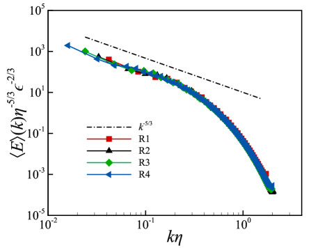
Figure 1: Mean energy spectra $\langle E\rangle(k)$ of the base flow. Dash-dotted line: the $k^{-5/3}$ power law.

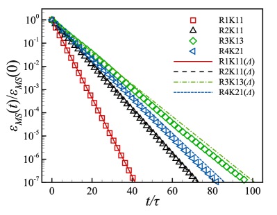
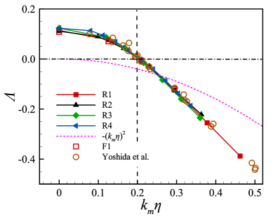
Figure 2: Left: Comparison between the decay rates of the synchronisation error ${\mathcal{E}}_{MS}(t)$ and the conditional LLEs. Right: Normalised conditional LLEs $\Lambda\equiv\lambda\tau$, with the short-dashed line showing $-(k_{m}\eta)^{2}$ and the vertical line marking $k_{m}\eta=0.2$. Only four data points are shown for the case F1. The empty circles are the decay rate data from Yoshida et al. (2005) (see the main text for more detail).

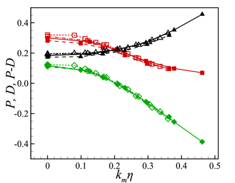
Figure 3: The production $P$, dissipation $D$ and $P-D$ as functions of $k_{m}\eta$. $P$: lines with both solid and empty squares; $D$: lines with both solid and empty triangles; $P-D$: lines with both solid and empty diamonds. Solid lines: R1; long dashed lines: R2; dash-dotted lines: R3; short-dashed lines: R4.

We start with a few results that characterise the basic properties of the flows and the synchronisation process. For reference, the average energy spectra are documented in Fig. 1, which is compared with the $k^{-5/3}$ scaling law. To monitor the synchronisation between ${\bm{u}}^{(M)}$ and ${\bm{u}}^{(S)}$, we use the synchronisation error

$${\mathcal{E}}_{MS}(t)=\|{\bm{u}}^{(M)}-{\bm{u}}^{(S)}\|,$$ (35)

which will decay exponentially when the two flows synchronise, and the rate of decay of ${\mathcal{E}}_{MS}$ is related to the conditional LLE $\lambda(k_{m})$, as having been shown in Henshaw et al. (2003); Yoshida et al. (2005); Inubushi et al. (2023); Li et al. (2024b). The left panel of Fig. 2 compares the results for ${\mathcal{E}}_{MS}(t)$ (symbols) with $\exp(\Lambda t/\tau)$ (lines), where

$$\Lambda(k_{m})\equiv\lambda(k_{m})\tau$$ (36)

is the conditional LLE non-dimensionalised with $\tau$. Some small discrepancies can be seen between the two quantities, which we attribute to statistical uncertainty. This result is consistent with previous findings (Nikolaidis & Ioannou, 2022; Li et al., 2024b), which shows that the non-dimensional decay rate of the synchronisation error can be given by $\Lambda$.

The right panel of Fig. 2 shows $\Lambda$ as functions of $k_{m}\eta$. The conditional LLEs are known to depend on the Reynolds number weakly (see, e.g., Inubushi et al. (2023)). Here the curves for different $Re_{\lambda}$ show some differences at small $k_{m}\eta$, but they collapse on each other for larger $k_{m}\eta$ (for, e.g., $k_{m}\eta\geq 0.15$) because $Re_{\lambda}$ varies only mildly. The conditional LLEs decrease as $k_{m}\eta$ increases, but the variation appears to be small for small $k_{m}\eta$. The threshold wavenumber $k_{c}$, for which $\Lambda=0$, is found to be $k_{c}\eta\approx 0.2$, which is also the value obtained in Yoshida et al. (2005) for isotropic turbulence. The dashed line without symbols is the function $-(k_{m}\eta)^{2}$, which is an estimate of the non-dimensional conditional LLE when the evolution of the velocity perturbation is determined solely by viscous diffusion (see, e.g., Inubushi et al. (2023)). We will discuss this estimate below together with Fig. 3.

The right panel of Fig. 2 also includes data from two other sources to cross check the results from groups R1-R4. The conditional LLEs from case F1 at four different $k_{m}\eta$ are plotted with empty squares. They display only negligible differences with those from R1, which shows that the results are essentially grid independent. The empty circles are calculated from the decay rates $\tilde{\alpha}$ obtained in Yoshida et al. (2005), plotted in Fig. 3 therein. More specifically, the empty circles are the values of $-\tilde{\alpha}/2$. Per Yoshida et al. (2005), $\tilde{\alpha}$ is defined by $\|{\bm{u}}^{(M)}-{\bm{u}}^{(S)}\|^{2}\sim\exp(-\tilde{\alpha}t/\tau)$. Since $\|{\bm{u}}^{(M)}-{\bm{u}}^{(S)}\|\sim\exp(\Lambda t/\tau)$ as is shown in the left panel of Fig. 2, we expect $\Lambda=-\tilde{\alpha}/2$. This relation is verified by the data, as the empty circles fall closely on the curves for $\Lambda$. Note that the empty circles correspond to a wide range of Reynolds numbers. Also, $\tilde{\alpha}$ is obtained by measuring the decay rate of $\|{\bm{u}}^{(M)}-{\bm{u}}^{(S)}\|^{2}$, which is a procedure that is very different from how $\Lambda$ is calculated (Yoshida et al., 2005). Thus, the agreement between $\Lambda$ and $-\tilde{\alpha}/2$ is a strong validation of our results.

Further insights on $\Lambda$ can be explored according to Eq. (17). We use

$$P\equiv\tau\left\langle{\mathcal{P}}_{e}\right\rangle,\qquad D\equiv\tau\left\langle{\mathcal{D}}_{e}\right\rangle$$ (37)

to denote the non-dimensional mean production and mean dissipation, respectively. It follows from Eq. (17) that

$$\Lambda=P-D.$$ (38)

Note that a pre-requisite for Eq. (38) is that the external forcing has no impact on the evolution of the velocity perturbation (c.f. Eq. (6) and the comments following Eq. (7)). Otherwise, the equation would contain a forcing term.

The values of $P$, $D$, and their difference $P-D$ are shown in Fig. 3 for different coupling wavenumber $k_{m}$. As dictated by Eq. (38), the curves for $P-D$ agree precisely with those of the conditional LLEs $\Lambda$ shown in Fig. 2 (the right panel thereof). The main observation about Fig. 3 is that $P$ decreases, whilst $D$ increases, with increasing $k_{m}$. The two curves intersect at the threshold wavenumber $k_{c}\eta$. Both seem to contribute roughly equally to the change in $\Lambda$ as $k_{m}$ varies. The results are slightly different for different $Re_{\lambda}$.

We now return to the discussion of the estimate $-(k_{m}\eta)^{2}$ for $\Lambda(k_{m})$ shown in Fig. 2. It was found in Inubushi et al. (2023) that $\Lambda(k_{m})$ is always larger than $-(k_{m}\eta)^{2}$, and approaches $-(k_{m}\eta)^{2}$ from above (see Fig. 3 therein). These trends suggest that $P$ becomes negligible for large $k_{m}\eta$, and $D$ approaches the pure viscous estimate as $k_{m}\eta$ increases. Our results, on the other hand, appear to display different behaviours, as we can see from Figs. 2 and 3. Firstly, Fig. 2 shows that $-(k_{m}\eta)^{2}$ can be larger than $\Lambda(k_{m})$ in our simulations. Secondly, Fig. 3 shows that, though $P$ decreases as $k_{m}\eta$ increases, it is still significantly larger than zero for the largest $k_{m}\eta$, even when $\Lambda(k_{m})$ is already smaller than $-(k_{m}\eta)^{2}$. In sum, the dissipation contribution in our simulations is significantly higher than what is implied by the estimate $-(k_{m}\eta)^{2}$. The cause for the difference is unclear. An explanation possibly, though unlikely, lies in the difference in the Reynolds numbers. We will discuss this further in Section 4.2 when we discuss the spectral dynamics of the LLVs.

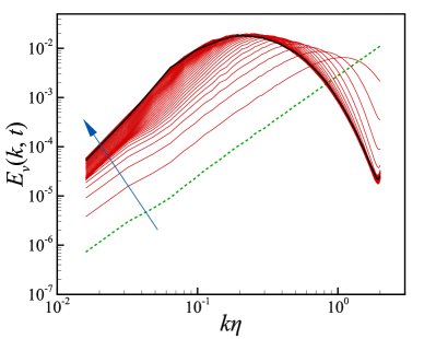
Figure 4: Left: Short time evolution of $E_{v}(k,t)$ for $t$ between $0$ and approximately $20\tau$, with the dashed line showing $E_{v}(k,t=0)$ and the black thick line showing $E_{v}(k,t)$ for $t\approx 20\tau$. The arrow indicates the increasing direction of time. Right: average energy spectra $\langle E_{v}\rangle$ for the unconditional LLV, with the vertical dashed line marking the value $k\eta=0.2$.

Finding the threshold wavenumber $k_{c}$ via the conditional LLEs requires considerable computational cost, as it entails calculating $\lambda(k_{m})$ for many $k_{m}$. On this issue, Li et al. (2024b) made an interesting observation in the context of rotating turbulence. They found that the average energy spectrum of the unconditional LLV peaks at a wavenumber which appears to be close to, or the same as $k_{c}$. The observation is reproduced in Li et al. (2024a) for the synchronisation of large eddy simulations of periodic turbulence. Elementary results for the spectra of the LLV in the present study, i.e., $E_{v}(k,t)$, are shown in Fig. 4. In the left panel of Fig. 4, the early evolution of $E_{v}(k,t)$ is plotted. We initialise the Fourier modes of the perturbation with independent random numbers with identical probability distributions. As a consequence, $E_{v}(k,t=0)\sim k^{2}$ for large $k$, as the number of modes in the spherical shell with radius $k$ is proportional to the area $4\pi k^{2}$ of the shell. $E_{v}(k,0)$ is shown with the green dashed line. The spectrum at time $t$, $E_{v}(k,t)$, exhibits a period of transient evolution, as depicted by the think red lines, which show that the peak of the spectrum moves towards lower wavenumbers. At $t\approx 20\tau$, the spectrum converges towards a distribution shown with the thick black line, which then fluctuates over time. The long time average $\langle E_{v}\rangle$ is shown in the right panel of Fig. 2. Clearly, the peaks of the spectra are found at $k\eta\approx 0.2$, reproducing previous findings. The flow here is very different from the rotating turbulence investigated in Li et al. (2024b). For example, the base flow energy spectrum $\langle E\rangle(k)$ follows the $k^{-2}$ or $k^{-3}$ power laws in Li et al. (2024b), whereas here it follows the canonical $k^{-5/3}$ scaling. Therefore, it is non-trivial for the same relationship to hold in both cases. As a step towards understanding the origin of this relationship, we look into the spectral dynamics of the LLVs and the conditional LLVs in what follows.

4.2 Production and dissipation: spectral analyses

To understand the dependence of $P$ and $D$ (hence $\Lambda$) on $k_{m}$ better, we look into the production spectrum ${\mathcal{P}}_{v}(k,t)$ and the dissipation spectrum ${\mathcal{D}}_{v}(k,t)$. We first consider their non-dimensional ensemble averages

$$P_{v}(k)\equiv\tau\langle{\mathcal{P}}_{v}(k,t)\rangle,\qquad D_{v}(k)\equiv\tau\langle{\mathcal{D}}_{v}(k,t)\rangle.$$ (39)

The expression for $D_{v}(k)$ can also be written as

$$D_{v}(k)=2\bar{\nu}k^{2}\tau\langle E_{v}\rangle(k)=2(k\eta)^{2}\langle E_{v}\rangle(k).$$ (40)

The behaviours of $P_{v}$ and $D_{v}$ are related by Eq. (27). Taking the average of Eq. (27), and noting $\partial_{t}\langle E_{v}\rangle=0$, we find

$$P_{v}(k)-D_{v}(k)=2\tau\langle\gamma E_{v}\rangle.$$ (41)

Our data show that $\gamma$ is essentially uncorrelated to $E_{v}$ (figure omitted). Therefore $\langle\gamma E_{v}\rangle\approx\langle\gamma\rangle\langle E_{v}\rangle=\lambda\langle E_{v}\rangle$, and we obtain

$$P_{v}(k)=D_{v}(k)+2\Lambda\langle E_{v}\rangle=2\left[(k\eta)^{2}+\Lambda(k_{m})\right]\langle E_{v}\rangle.$$ (42)

The equation delineates the spectral balance of the energetics of the velocity perturbation. Integrating Eq. (42) over $k$, we obtain

$$\Lambda(k_{m})=\int_{0}^{\infty}P_{v}(k)dk-\int_{0}^{\infty}2(k\eta)^{2}\langle E_{v}\rangle(k)dk,$$ (43)

which makes clear that Eq. (43) is the spectral version of Eq. (38).

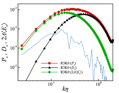
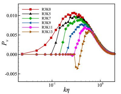
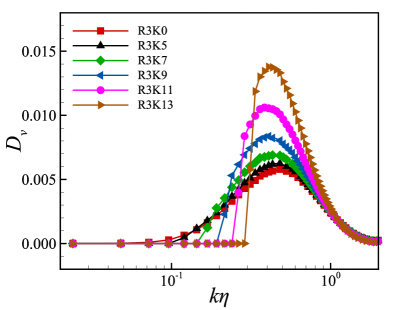
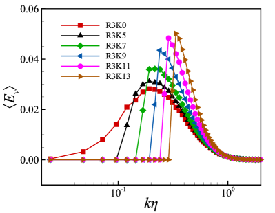
Figure 5: Top-left: production spectrum $P_{v}$, dissipation spectrum $D_{v}$ and $2\Lambda\langle E_{v}\rangle$ as a function of $k\eta$ for $k_{m}=0$ with the dashed line showing the residual $P_{v}-D_{v}-2\Lambda\langle E_{v}\rangle$. Top-right: $P_{v}$. Bottom-left: $D_{v}$. Bottom-right: $\langle E_{v}\rangle$. The non-dimensionalised coupling wavenumbers $k_{m}\eta$ are $0$, $0.12$, $0.17$, $0.22$, $0.26$, and $0.31$. For group R3.

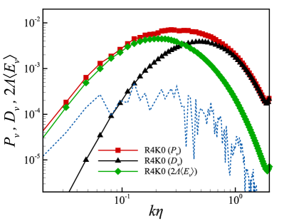
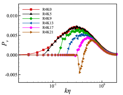
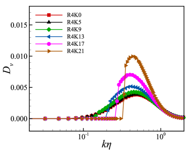
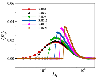
Figure 6: Same as Fig. 5 but for group R4. The non-dimensionalised coupling wavenumbers $k_{m}\eta$ are $0$, $0.08$, $0.14$, $0.21$, $0.27$, and $0.34$.

Fig. 5 shows the spectra $P_{v}$, $D_{v}$, and $\langle E_{v}\rangle$ with different $k_{m}$ for the cases in group R3. The same results for group R4 are shown in Fig. 6 as corroboration. The two figures depict same behaviours. Therefore we will only discuss Fig. 5 in detail. The top-left panel of Fig. 5 compares the three distributions for $k_{m}=0$, i.e., for the cases where no coupling is imposed. The dashed line shows the residual $P_{v}-D_{v}-2\Lambda\langle E_{v}\rangle$, which, according to Eq. (42), should be essentially zero. Though it is not exactly zero, the dashed line shows that it is negligible compared with the dominant terms at all wavenumbers. Not surprisingly, the dissipation $D_{v}$ peaks at a higher wavenumber compared with $P_{v}$ and $2\Lambda\langle E_{v}\rangle$, as dissipation dominantly comes from small scales. On the other hand, $2\Lambda\langle E_{v}\rangle$ peaks at $k\eta\approx 0.2$ (same as that of $\langle E_{v}\rangle$). The peak of $P_{v}$ is found at a wavenumber in between, which shows that the strongest production is found at wavenumbers well inside the dissipation range of the base flow. Also, $P_{v}(k)$ is positive definite, implying that the velocity perturbation is amplified by the production mechanism at all scales.

The production spectra for several different $k_{m}$ are shown in the top-right panel of Fig. 5. Because $\hat{{\bm{v}}}({\bm{k}},t)=0$ for $|{\bm{k}}|<k_{m}$ due to the coupling between the synchronised flows, $P_{v}(k)=0$ for $k<k_{m}$. What is noteworthy is that $P_{v}(k)$ is also reduced by the coupling for $k>k_{m}$, and it is increasingly smaller for larger $k_{m}$. The attenuating effect of the coupling is localised in the wavenumbers around $k_{m}$, with $P_{v}(k)$ at large $k$ little affected. To interpret this feature, we refer back to Eq. (29). Since $\hat{{\bm{v}}}(\bm{q},t)=0$ when $|\bm{q}|<k_{m}$, the summation in Eq. (29) does not include the Fourier modes with $|\bm{q}|<k_{m}$. Thus increasing $k_{m}$ means excluding more Fourier modes from the summation, which thus likely leads to smaller $P_{v}(k)$, because the top-left panel shows that the contributions from these excluded modes are likely to be positive.

Another observation is that, though $P_{v}(k)$ is positive definite for $k>k_{m}$ in most cases, it assumes negative values for some wavenumbers when $k_{m}$ is large enough (e.g. for case R$3$K$13$). This observation can be understood from Eq. (42). Obviously, $P_{v}(k)$ would be positive definite for $k>k_{m}$ if $(k\eta)^{2}+\Lambda(k_{m})>0$ for all $k>k_{m}$. This is clearly satisfied if $\Lambda(k_{m})>0$, which is the case when $k_{m}=0$ or $k_{m}$ is small. If $\Lambda(k_{m})<0$, on the other hand, then $(k\eta)^{2}+\Lambda<0$ when $k\eta<(-\Lambda)^{1/2}$. As a result, $P_{v}(k)$ would be negative for wavenumber $k$ if $k_{m}\eta<k\eta<(-\Lambda)^{1/2}$. The inequality can be satisfied by some wavenumbers if $-(k_{m}\eta)^{2}>\Lambda(k_{m})$, which is satisfied when $k_{m}\eta$ is large enough as shown in the right panel of Fig. 2. Therefore, when $k_{m}$ is large enough, the velocity perturbations at the scales just below the coupling scale would be suppressed by the production term.

The dissipation spectrum $D_{v}$ is shown in the bottom-left panel, while the energy spectrum $\langle E_{v}\rangle$ is shown in the bottom-right panel. As $D_{v}=2(k\eta)^{2}\langle E_{v}\rangle$, the two parameters are similar in many ways. The most conspicuous feature for both is that their distributions are elevated as $k_{m}$ increases. This behaviour could be a simple consequence of the normalisation condition $\langle e\rangle_{v}=1/2$ which fixes the total integral of $\langle E_{v}\rangle$. As the support of $\langle E_{v}\rangle$ is reduced when $k_{m}$ increases, its values have to increase. The values of $D_{v}(k)$, as a consequence, have to increase too. Nevertheless, there is another mechanism by which $D_{v}(k)$ is enhanced. Eq. (42) implies that

$$D_{v}(k)=P_{v}(k)\frac{(k\eta)^{2}}{(k\eta)^{2}+\Lambda(k_{m})}.$$ (44)

The above equation shows that reduced $P_{v}(k)$ tends to reduce $D_{v}(k)$. However, reduced $P_{v}(k)$ also tends to reduce $\Lambda(k_{m})$, which in turns enhances the factor $(k\eta)^{2}/[\Lambda(k_{m})+(k\eta)^{2}]$, thus potentially increases $D_{v}(k)$. That is, there is a mechanism by which $D_{v}(k)$ increases as a consequence of reduced $P_{v}(k)$. This effect is stronger at lower wavenumbers as the factor $(k\eta)^{2}/[\Lambda(k_{m})+(k\eta)^{2}]$ is more sensitive to the change in $\Lambda(k_{m})$ when $k\eta$ is smaller. Unfortunately, it is unclear which of the above two mechanisms contributes more to the enhancement of $D_{v}(k)$.

We now turn to a brief discussion on the viscous estimate $-(k_{m}\eta)^{2}$ for $\Lambda(k_{m})$. Note that $\langle E_{v}\rangle(k)=0$ for $k<k_{m}$. Therefore,

$$D =\int_{k_{m}}^{\infty}2(k\eta)^{2}\langle E_{v}\rangle dk=2(k_{m}\eta)^{2}\int_{k_{m}}^{\infty}(k/k_{m})^{2}\langle E_{v}\rangle dk$$

$$\geq 2(k_{m}\eta)^{2}\int_{k_{m}}^{\infty}\langle E_{v}\rangle dk=(k_{m}\eta)^{2},$$ (45)

which implies that $(k_{m}\eta)^{2}$ tends to underestimate the dissipation $D$. Therefore, it might not be surprising that in our simulations $\Lambda(k_{m})$ becomes smaller than $-(k_{m}\eta)^{2}$ for some $k_{m}$. The estimate $(k_{m}\eta)^{2}$ would, however, become exact if $\langle E_{v}\rangle$ was proportional to the Dirac delta function concentrated at $k_{m}$ (with the strength being $1/2$). Our results in the bottom-right panel of Fig. 5 do show a tendency for $\langle E_{v}\rangle$ to concentrate around $k_{m}$ as $k_{m}$ increases.

We have been able to present some semi-analytical discussions of the results in Fig. 5 based on Eq. (42). Deriving the relationship between the coupling wavenumber $k_{c}\eta$ and the peak wavenumber of $\langle E_{v}\rangle$ analytically requires, as a very first step, finding an analytical expression for the peak wavenumber for $\langle E_{v}\rangle$ at $k_{m}=0$. Attempts at such analyses, however, quickly run into the classical closure problem, as we do not have an expression for $P_{v}(k)$ in terms of $\langle E_{v}\rangle$. Nevertheless, some elementary results can be obtained. Since the peak wavenumber is given by $d\langle E_{v}\rangle/d(k\eta)=0$, we can find from $\langle E_{v}\rangle=P_{v}(k)/[2(k\eta)^{2}+2\Lambda(0)]$ that the peak wavenumber $k\eta$ satisfies

$$\frac{2k\eta}{(k\eta)^{2}+\Lambda(0)}=\frac{1}{P_{v}}\frac{dP_{v}}{d(k\eta)}=\frac{d\ln P_{v}}{d(k\eta)},$$ (46)

which can be solved for $k\eta$ if we have an expression for $P_{v}(k)$. Purely as a demonstration, we let $P_{v}(k)\sim a(k\eta)^{b}$, assuming the expression provides a good approximation for the slope of $\ln P_{v}(k)$ around the peak wavenumber for some constants $a$ and $b$. The peak wavenumber is then given by

$$k\eta=\left(\frac{b\Lambda(0)}{2-b}\right)^{1/2}.$$ (47)

If we let $\Lambda(0)=0.12$ (hence ignoring $\Lambda(0)$’s dependence on $Re_{\lambda}$), then $b=1/2$ would give $k\eta=0.2$. Progress may be made by developing an EDQNM-type model for $P_{v}(k)$, but this is beyond the scope of this investigation.

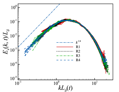
Figure 7: Normalised spectrum $E_{v}(k,t)/L_{\delta}$ as a function of $kL_{\delta}$ at different times. For cases with $k_{m}=0$ only.

We now explore some aspects of the time evolution of the spectrum $E_{v}(k,t)$. An interesting observation is made in Ge et al. (2023); Yoshimatsu & Ariki (2019), which shows that $E_{\delta}(k,t)$ evolves in a self-similar manner over a period of time. To examine this phenomenon in our simulations, we follow Ge et al. (2023), and define an integral length scale for the velocity perturbation by

$$L_{\delta}(t)=\frac{3\pi}{4K_{\delta}(t)}\int_{0}^{\infty}k^{-1}E_{\delta}(k,t)dk=\frac{3\pi}{2}\int_{0}^{\infty}k^{-1}E_{v}(k,t)dk.$$ (48)

Self-similar evolution takes place if $E_{\delta}(k,t)/K_{\delta}L_{\delta}$ is a function of $kL_{\delta}$ alone, independent of time. In terms of $E_{v}(k,t)$, it implies that we have

$$E_{v}(k,t)=L_{\delta}(t)g(kL_{\delta}),$$ (49)

for some function $g(\cdot)$. Eq. (49) implies that, $E_{v}/L_{\delta}$, when plotted against $kL_{\delta}$, should collapse on a single curve. Fig. 7 plots the results obtained from our data over a period of time spanning over $100\tau$. The immediate observation is that the curves mostly fall on each other. The agreement is the best for wavenumbers somewhat larger than the wavenumber where the curves peak. This feature is also observed in Ge et al. (2023). The discrepancies are larger at the two ends of the spectra. The peak of the normalised spectra is found approximately at $kL_{\delta}=2$, the same as in Ge et al. (2023). There are attempts to deduce analytically the slope of the spectra as $kL_{\delta}\to 0$ (Yoshimatsu & Ariki, 2019), but various values have been observed in DNS. For example, $k^{4}$ is found in Yoshimatsu & Ariki (2019), and slopes closer to $k^{3.3}$ are reported in Ge et al. (2023). For the cases in group R4, which have the largest Reynolds number in our simulations, the slope appears to scale with $k^{2.8}$, as shown by the dash-double-dotted line.

Our observation broadly agrees with those in Ge et al. (2023); Yoshimatsu & Ariki (2019). Note that the spectra shown in Fig. 7 are calculated from the long time limit of ${\bm{v}}$. In contrast, Ge et al. (2023); Yoshimatsu & Ariki (2019) observe self-similarity in an intermediate stage of the evolution of the velocity perturbation where no rescaling is applied to keep the perturbation small. The agreement between the results shows that the intermediate stage of evolution observed in the latter appears to be the same as the long time asymptotic state of an infinitesimal perturbation.

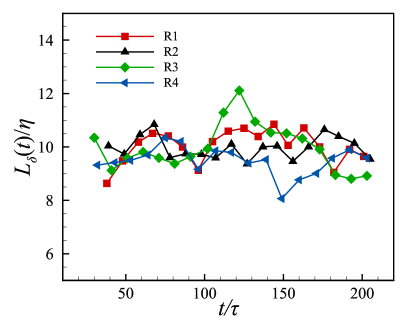
Figure 8: Normalised integral length scale $L_{\delta}/\eta$ for the perturbation velocity.

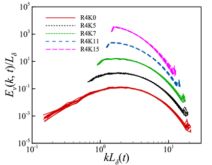
Figure 9: Normalised instantaneous energy spectrum $E_{v}(k,t)/L_{\delta}$ as a function of $kL_{\delta}$ for different $k_{m}$ at different times. For cases in group R4.

It is natural to explore the relationship between the peak location of the self-similar spectrum and the peak location of $\langle E_{v}\rangle$ shown in the right panel of Fig. 4. This can be inferred from Fig. 8, which shows that the ratio $L_{\delta}/\eta$ fluctuates around $10$. Therefore $kL_{\delta}\approx 2$ is equivalent to $k\eta\approx 0.2$, which is the peak location of $\langle E_{v}\rangle(k)$. This relationship lends further support to the conjecture that the peak wavenumber of $\langle E_{v}\rangle$ is a physically significant parameter for turbulence synchronisation. Another finding is that self-similarity is also observed for the spectra of the conditional LLVs, as shown in Fig. 9. For clarity, the curves for larger $k_{m}$ are shift upwards by a factor of $10$ successively. Evidently, there is a very good agreement between the curves at different times, as required by self-similarity.

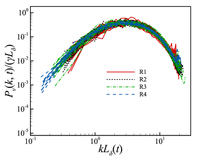
Figure 10: Normalised instantaneous production spectrum $P_{v}(k,t)/(\gamma L_{\delta})$ as a function of $kL_{\delta}$. For cases with $k_{m}=0$ only.

The self-similar evolution can be examined quantitatively via the equation for the spectrum $E_{v}(k,t)$, i.e., Eq. (27). Substituting Eq. (49) into Eq. (27), we obtain

$$g(\xi)+\xi\frac{dg}{d\xi}=\frac{P_{v}(k,t)}{\dot{L}_{\delta}}-\frac{2\bar{\nu}}{L_{\delta}\dot{L}_{\delta}}\xi^{2}g(\xi)-\frac{\gamma(t)L_{\delta}(t)}{\dot{L}_{\delta}}g(\xi),$$ (50)

where $\xi\equiv kL_{\delta}$ and $\dot{L}_{\delta}$ is the time derivative of $L_{\delta}$. Therefore, a fully self-similar solution (over all wavenumbers) is possible only if

$$\frac{P_{v}(k,t)}{\dot{L}_{\delta}}=h(\xi),\qquad\frac{2\bar{\nu}}{L_{\delta}\dot{L}_{\delta}}=\alpha,\qquad\frac{\gamma(t)L_{\delta}(t)}{\dot{L}_{\delta}}=\beta,$$ (51)

where $h(\xi)$ is some function to be determined, and $\alpha$ and $\beta$ are constants. Fig. 7 shows that $E_{v}(k,t)$ is mainly self-similar for intermediate wavenumbers. For these wavenumbers, we may drop the viscous effect, i.e., the second term on the right hand side of Eq. (50). With that, only the first and the third equations in Eq. (51) are required for there to be a self-similar solution. The third equation establishes a relation between $\gamma(t)$ and $L_{\delta}(t)$. It shows that $L_{\delta}$ grows exponentially if $\gamma(t)$ is a constant. The growth rate of $L_{\delta}$ is given by $\gamma/\beta$ and $L_{\delta}\sim\exp(\gamma t/\beta)$. This regime appears to be the one observed in Ge et al. (2023). However, Fig. 8 shows that $L_{\delta}(t)$ does not grow exponentially for our data (and $\gamma(t)$ is generally not a constant). Therefore, the self-similarity in our data belongs to a different regime, characterised more generally by the third equation in Eq. (51).

In order for the self-similar solution to exist, $P_{v}(k,t)$ must also have a self-similar form, as shown by the first equation in Eq. (51). Together with the third equation in Eq. (51), we obtain

$$P_{v}(k,t)=\dot{L}_{\delta}h(\xi)=\beta^{-1}\gamma(t)L_{\delta}(t)h(\xi)\sim\gamma(t)L_{\delta}(t)h(\xi).$$ (52)

We plot $P_{v}(k,t)/(\gamma(t)L_{\delta}(t))$ against $kL_{\delta}$ in Fig. 10. The agreement between the curves at different times is less satisfactory compared with that shown in Fig. 7, but the curves still largely fall on each other. The deviation from a clear self-similarity in $P_{v}$ could be due to the contamination from the two ends of $E_{v}(k,t)$. Note that $E_{v}(k,t)$ is self-similar mainly in the mid-wavenumber range, which means $g(\xi)$ is well-defined only for a finite range of values for $\xi$. Since $h(\xi)\sim dg/d\xi$ according to Eq. (50), it is plausible that $h(\xi)$ is well defined over a narrower range of $\xi$. This argument suggests that simulations covering a wider range of wavenumbers are required to ascertain whether strict self-similarity in $P_{v}(k,t)$ exists or not.

4.3 Production and dissipation: physical space analyses

Additional understanding of the production and dissipation of the LLV can be obtained with complementary analyses in the physical space. It has been known for a while that the spatial structures of the velocity perturbations (Nikitin, 2008, 2018; Ge et al., 2023) are non-trivial. Physical space analyses are well-suited if one is interested in the impacts of these spatial structures.

In physical space analyses, it is more meaningful to express the production term in the intrinsic coordinates formed by the eigenvectors of the strain rate tensor. Let $s^{+}_{ij}\equiv\tau s_{ij}$ be the non-dimensional strain rate tensor, so that we can write $P=-\langle v_{i}v_{j}s^{+}_{ij}\rangle$. We let $\lambda_{\alpha}\geq\lambda_{\beta}\geq\lambda_{\gamma}$ be the eigenvalues of $s^{+}_{ij}$, with corresponding eigenvectors ${\bm{e}}_{i}$ $(i=\alpha,\beta,\gamma)$. Due to incompressibility, we have $\lambda_{\alpha}+\lambda_{\beta}+\lambda_{\gamma}=0$. Thus $\lambda_{\alpha}$ is always non-negative whereas $\lambda_{\gamma}$ is always non-positive. Letting $\theta_{i}$ be the angle between ${\bm{e}}_{i}$ and ${\bm{v}}$, we may write

$$P=P_{\alpha}+P_{\beta}+P_{\gamma},$$ (53)

with

$$P_{\alpha}=-2\left\langle e\lambda_{\alpha}\cos^{2}\theta_{\alpha}\right\rangle,\quad P_{\beta}=-2\left\langle e\lambda_{\beta}\cos^{2}\theta_{\beta}\right\rangle,\quad P_{\gamma}=-2\left\langle e\lambda_{\gamma}\cos^{2}\theta_{\gamma}\right\rangle.$$ (54)

Eq. (54) captures the fact that the production hinges on the correlation among the eigenvalues of $s^{+}_{ij}$, the alignment between ${\bm{v}}$ and the eigenvectors, and the magnitude of ${\bm{v}}$.

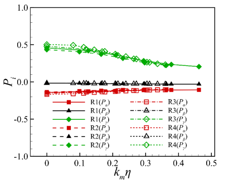
Figure 11: The $P_{\alpha}$, $P_{\beta}$ and $P_{\gamma}$ components of the mean production $P$ as functions of $k_{m}\eta$.

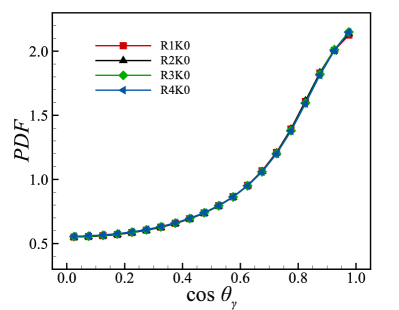
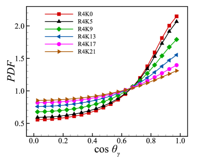
Figure 12: The PDFs of $\cos\theta_{\gamma}$. Left: cases from all groups with $k_{m}=0$. Right: cases in group R4 with different $k_{m}$.

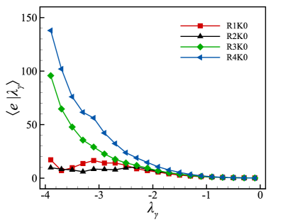
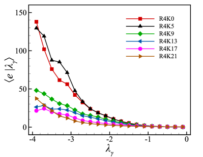
Figure 13: The conditional average $\langle e|\lambda_{\gamma}\rangle$ as a function of $\lambda_{\gamma}$. Left: cases from all groups with $k_{m}=0$. Right: cases in group R4 with different $k_{m}$.

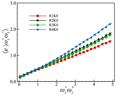
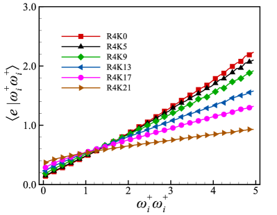
Figure 14: The conditional average $\langle e|\omega_{i}^{+}\omega_{i}^{+}\rangle$. Left: cases from all groups with $k_{m}=0$. Right: cases in group R4 with different $k_{m}$.

The production components $P_{\alpha}$, $P_{\beta}$, and $P_{\gamma}$ as functions of $k_{m}\eta$ are shown in Fig. 11. One can observe that $P_{\alpha}$, $P_{\beta}$, and $P_{\gamma}$ exhibit negligible dependence on $Re_{\lambda}$. As expected, $P_{\alpha}<0$ and $P_{\gamma}>0$. We also observe $P_{\beta}<0$ with much smaller magnitudes, and $P_{\gamma}$ is the dominant one among the three terms. Of particular note is that $P_{\alpha}$ and $P_{\beta}$ are nearly independent of $k_{m}\eta$, whereas $P_{\gamma}$ decreases as $k_{m}\eta$ increases. Thus, the change in $P$ with respect to $k_{m}\eta$ (as shown in Fig. 3) is predominantly due to the contribution from $P_{\gamma}$. As a result, we focus on $P_{\gamma}$ only in what follows.

Fig. 12 presents the PDF of $\cos\theta_{\gamma}$. As can be observed in the left panel of Fig. 12, results for different Reynolds numbers are essentially the same. The PDFs increase with $\cos\theta_{\gamma}$, suggesting a strong tendency for the eigenvector ${\bm{e}}_{\gamma}$ to align with the vector ${\bm{v}}$. There are noticeable differences between the PDFs for different $k_{m}$, as shown on the right panel of Fig. 12. As $k_{m}$ increases, the preferential alignment between ${\bm{e}}_{\gamma}$ and ${\bm{v}}$ is weakened, manifested in the lower peaks. This behaviour clearly is one of the reasons why $P$ decreases with $k_{m}$ as shown in Fig. 3. The PDFs at other Reynolds numbers exhibit similar trends, thus not shown to avoid redundancy. The behaviours shown in the right panel of Fig. 12 can be qualitatively understood from the characteristics length scales or wavenumbers of $s^{+}_{ij}$ and $v_{i}$. The characteristic wavenumber of $s^{+}_{ij}$ can be estimated by the wavenumber where the dissipation spectrum of the base flow peaks, which is found to be approximately $0.15\eta^{-1}$. The characteristic wavenumber for $v_{i}$ can be estimated by $\max(0.2\eta^{-1},k_{m})$, with $0.2\eta^{-1}$ being the peak wavenumber for $\langle E_{v}\rangle$ when it is bigger than $k_{m}$. Thus, as $k_{m}$ increases, the mismatch between the two characteristic wavenumbers tends to increases, which tends to weaken the correlation between $s^{+}_{ij}$ and $v_{i}$, hence the alignment in Fig. 12 (right).

Incidentally, the preferential alignment discussed above is reminiscent of the behaviours of the gradient of a passive scalar in isotropic turbulence, which also tends to align with ${\bm{e}}_{\gamma}$ of the strain rate tensor (Ashurst et al., 1987). However, the statistics of ${\bm{v}}$ are different from those of a passive scalar on many aspects, as we can see from the statistics of $B_{ij}$ which will be discussed later.

The impacts of the correlation between the perturbation and the strain rate tensor can be explored with suitable conditional statistics. Note that

$$P_{\gamma}=-2\int\langle e\cos^{2}\theta_{\gamma}|\lambda_{\gamma}\rangle\lambda_{\gamma}f_{\gamma}(\lambda_{\gamma})d\lambda_{\gamma},$$ (55)

where $f_{\gamma}(\lambda_{\gamma})$ is the PDF of the eigenvalue $\lambda_{\gamma}$. Therefore, how the correlation between the $\lambda_{\gamma}$, the alignment, and $e$ contributes to $P_{\gamma}$ can be understood from the conditional average $\langle e\cos^{2}\theta_{\gamma}|\lambda_{\gamma}\rangle$. Our tests show that $\langle e\cos^{2}\theta_{\gamma}|\lambda_{\gamma}\rangle$ tends to be smaller than $\langle e|\lambda_{\gamma}\rangle$ due to the factor $\cos^{2}\theta_{\gamma}$, but the two distributions display similar shapes. To keep the discussion succinct, we consider only $\langle e|\lambda_{\gamma}\rangle$, which is shown in Fig. 13. The left panel, firstly, shows that $\langle e|\lambda_{\gamma}\rangle$ changes with the Reynolds number quite significantly, in contrast to the alignment trend shown in Fig. 12. The impact of the Reynolds numbers is especially strong for large $|\lambda_{\gamma}|$, where the conditional average generally is larger for larger Reynolds numbers. This behaviour is likely due to the fact that the probability for strong strain rate increases with the Reynolds number due to the intermittency effects. The right panel plots $\langle e|\lambda_{\gamma}\rangle$ for different $k_{m}$ with a fixed Reynolds number. The conditional average increases with $|\lambda_{\gamma}|$ for all $k_{m}$, but it is generally smaller for larger $k_{m}$. This behaviour is another factor by which $P$ decreases as $k_{m}$ increases, in addition to the weakened alignment shown in the right panel of Fig. 12. The reduction in $\langle e|\lambda_{\gamma}\rangle$ as $k_{m}$ increases may also be attributed to the mismatch between the characteristics length scales of $s^{+}_{ij}$ and $v_{i}$. Overall, Fig. 13 shows that the perturbation tends to be stronger at regions with stronger strain rate (shown with larger $|\lambda_{\gamma}|$), though it is reduced as $k_{m}$ increases.

The descriptions of the velocity perturbation can be further elaborated by considering the correlation between $e$ and the base flow vorticity. Let ${\bm{\omega}}=\nabla\times{\bm{u}}$ be the vorticity of the base flow, and ${\bm{\omega}}^{+}=\tau{\bm{\omega}}$ be the non-dimensionalised version of ${\bm{\omega}}$. Fig. 14 shows the conditional average $\langle e|\omega_{i}^{+}\omega_{i}^{+}\rangle$, which characterises the correlation between the magnitude of the perturbation and the vorticity of the base flow. When $k_{m}=0$, Fig. 14 shows that the conditional average increases with the magnitude of base flow vorticity, and it depends only weakly on the Reynolds number. When $k_{m}$ is increased, the dependence of $\langle e|\omega_{i}^{+}\omega_{i}^{+}\rangle$ on $\omega_{i}^{+}\omega_{i}^{+}$ is weakened. As a result, the conditional average increases with $k_{m}$ for smaller $\omega_{i}^{+}\omega_{i}^{+}$ and decreases with $k_{m}$ for larger $\omega_{i}^{+}\omega_{i}^{+}$. Therefore, perturbations associated with regions of strong vorticity in the base flow are stronger on average, and this trend tends to be weakened as the coupling wavenumber $k_{m}$ increases. The conditional average $\langle e|\omega_{i}^{+}\omega_{i}^{+}\rangle$ depends on the Reynolds number and $k_{m}$ in the same way as $\langle e|\lambda_{\gamma}\rangle$, thus its behaviours can be explained in a similar way. The correlation between $e$ and strong strain rate and strong vorticity is also observed in channel flows to some extent (Nikitin, 2018).

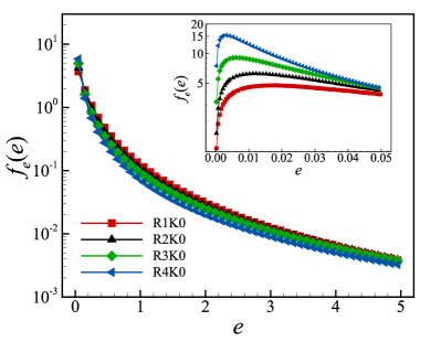
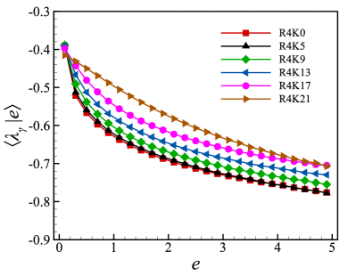
Figure 15: Left: PDFs $f_{e}(e)$ from all groups with $k_{m}=0$ with the inset showing the variation of the PDFs with the Reynolds number near $e=0$. Right: conditional average $\langle\lambda_{\gamma}|e\rangle$ for group R4 with different $k_{m}$.

To understand how the fluctuations in the perturbation velocity contribute to the mean production term, we may write the mean production as the weighted integral of the average conditioned on given $e$, i.e.,

$$P_{\gamma}=-2\int\langle\lambda_{\gamma}\cos^{2}\theta_{\gamma}|e\rangle ef_{e}(e)de,$$ (56)

where $f_{e}(e)$ is the PDF of $e$. The left panel of Fig. 15 plots $f_{e}(e)$ for different Reynolds numbers with $k_{m}=0$ only. The PDFs display very elongated tails, showing high probabilities for large fluctuations in $e$. The tail is very slightly fatter for higher Reynolds numbers. The peaks of the PDFs are found at small $e$ values, and they are slightly sharper for higher Reynolds numbers. The distributions indicate that the spatial distribution of the perturbation velocity is highly intermittent, with small fluctuations covering large part of the spatial domain and strong fluctuations observed in localised spots. The results for $\langle\lambda_{\gamma}|e\rangle$ are shown in the right panel of Fig. 15, The magnitude of the conditional average increases with $e$ and $k_{m}$. These behaviours are consistent with the results for $\langle e|\lambda_{\gamma}\rangle$. Given the highly intermittent nature of the distribution of $e$, one might ask how important are the large fluctuations to the mean production. Though its figure is omitted, one can readily see that the product $-\langle\lambda_{\gamma}\cos^{2}\theta_{\gamma}|e\rangle ef_{e}(e)\approx-\langle\lambda_{\gamma}|e\rangle ef_{e}(e)$, as a function of $e$, peaks at an intermediate value of $e$. Therefore, the main contribution to the mean production does not come from the very large fluctuations.

We now explore the behaviours of the dissipation term ${\mathcal{D}}_{e}$ in the physical space. Eq. (22) shows that ${\mathcal{N}}_{e}$ is one of the main mechanisms that determines the dissipation rate ${\mathcal{D}}_{e}$, and it will be the focus below. We let

$$N_{es}=\frac{\tau\langle{\mathcal{N}}_{es}\rangle}{\langle{\mathcal{D}}_{e}\rangle},\qquad N_{eo}=\frac{\tau\langle{\mathcal{N}}_{eo}\rangle}{\langle{\mathcal{D}}_{e}\rangle},$$ (57)

which are both dimensionless (c.f. Eq. (22)). Equivalently, we may introduce a length scale $(\bar{\nu}/\langle{\mathcal{D}}_{e}\rangle)^{1/2}$, and then define non-dimensional perturbation strain rate and perturbation vorticity, denoted by $s_{ij}^{-}$ and $\omega^{-}_{ij}$, respectively, with

$$s^{-}_{ij}=\frac{\bar{\nu}^{1/2}s^{v}_{ij}}{\langle{\mathcal{D}}_{e}\rangle^{1/2}},\qquad\omega^{-}_{ij}=\frac{\bar{\nu}^{1/2}\omega^{v}_{ij}}{\langle{\mathcal{D}}_{e}\rangle^{1/2}}.$$ (58)

Recalling that ${\bm{v}}$ is dimensionless, therefore the dimension of $s^{v}_{ij}$ and $\omega^{v}_{i}$ is that of the reciprocal of length, so that $s^{-}_{ij}$ and $\omega^{-}_{i}$ are dimensionless. As a consequence, we obtain

$$N_{es}=-4\langle s^{+}_{ij}s^{-}_{jk}s^{-}_{ki}\rangle,\quad N_{eo}=\langle s^{+}_{ij}\omega^{-}_{i}\omega^{-}_{j}\rangle.$$ (59)

In terms of $N_{es}$ and $N_{eo}$, we may re-write Eq. (24). Assuming the correlation between $\gamma$ and ${\mathcal{D}}_{e}$ is negligible, we obtain $\langle\gamma{\mathcal{D}}_{e}\rangle\approx\langle\gamma\rangle\langle{\mathcal{D}}_{e}\rangle=\lambda\langle{\mathcal{D}}_{e}\rangle$. Therefore, Eq. (24) becomes

$$2\Lambda\approx N_{es}+N_{eo}+r_{e}$$ (60)

where

$$r_{e}\equiv-\frac{2\bar{\nu}\tau\langle s^{v}_{ij}\partial^{2}_{ij}p_{e}\rangle}{\langle{\mathcal{D}}_{e}\rangle}-\frac{2\tau\langle\bar{\nu}\nabla B_{ij}\cdot\bar{\nu}\nabla B_{ij}\rangle}{\langle{\mathcal{D}}_{e}\rangle}+\frac{2\tau\bar{\nu}\langle B_{ij}\nabla\cdot({\bm{v}}A_{ij})\rangle}{\langle{\mathcal{D}}_{e}\rangle},$$ (61)

is considered a ‘residual’ term. Therefore, the values of $N_{eo}$ and $N_{es}$ can be compared with $2\Lambda$ to gauge their contributions.

The expression of $N_{eo}$ is similar to that of $P$ in form with $v_{i}$ replaced by $\omega^{-}_{i}$. It is also similar in form to the vortex stretching term $s_{ij}^{+}\omega^{+}_{i}\omega^{+}_{j}$ for the enstrophy of the base flow. Using the eigen-frame defined by the eigenvectors of $s^{+}_{ij}$ introduced previously, we may write

$$N_{eo}=N_{eo\alpha}+N_{eo\beta}+N_{eo\gamma},$$ (62)

with

$$N_{eo\alpha}=\langle\lambda_{\alpha}|{\bm{\omega}}^{-}|^{2}\cos^{2}\theta^{o}_{\alpha}\rangle,~N_{eo\beta}=\langle\lambda_{\beta}|{\bm{\omega}}^{-}|^{2}\cos^{2}\theta^{o}_{\beta}\rangle,~N_{eo\gamma}=\langle\lambda_{\gamma}|{\bm{\omega}}^{-}|^{2}\cos^{2}\theta^{o}_{\gamma}\rangle,$$ (63)

where $\theta^{o}_{i}$ ($i=\alpha,\beta,\gamma$) denotes the angle between ${\bm{\omega}}^{-}$ and ${\bm{e}}_{i}$. Eqs. (62) and (63) are similar to those for $P$. Similarly, $N_{es}$ has an expression in terms of the eigenvalues and eigenvectors of $s^{+}_{ij}$ and $s^{-}_{ij}$. Let ${\bm{e}}_{\ell}^{-}$ ($\ell=\alpha,\beta,\gamma$) be the eigenvectors of $s^{-}_{ij}$, with corresponding eigenvalues $\lambda^{-}_{\ell}$. We follow the same tradition where $\lambda^{-}_{\alpha}\geq\lambda^{-}_{\beta}\geq\lambda^{-}_{\gamma}$. Letting $\theta^{s}_{ij}$ be the angle between ${\bm{e}}^{-}_{i}$ and ${\bm{e}}_{j}$, we obtain

$$N_{es}=-4 \left[\langle(\lambda_{\alpha}^{-})^{2}\lambda_{\alpha}\cos^{2}\theta^{s}_{\alpha\alpha}\rangle+\langle(\lambda_{\alpha}^{-})^{2}\lambda_{\beta}\cos^{2}\theta^{s}_{\alpha\beta}\rangle+\langle(\lambda_{\alpha}^{-})^{2}\lambda_{\gamma}\cos^{2}\theta^{s}_{\alpha\gamma}\rangle\right.$$

$$+ \left.\phantom{[}\langle(\lambda_{\beta}^{-})^{2}\lambda_{\alpha}\cos^{2}\theta^{s}_{\beta\alpha}\rangle+\langle(\lambda_{\beta}^{-})^{2}\lambda_{\beta}\cos^{2}\theta^{s}_{\beta\beta}\rangle+\langle(\lambda_{\beta}^{-})^{2}\lambda_{\gamma}\cos^{2}\theta^{s}_{\beta\gamma}\rangle\right.$$

$$+ \left.\phantom{[}\langle(\lambda_{\gamma}^{-})^{2}\lambda_{\alpha}\cos^{2}\theta^{s}_{\gamma\alpha}\rangle+\langle(\lambda_{\gamma}^{-})^{2}\lambda_{\beta}\cos^{2}\theta^{s}_{\gamma\beta}\rangle+\langle(\lambda_{\gamma}^{-})^{2}\lambda_{\gamma}\cos^{2}\theta^{s}_{\gamma\gamma}\rangle\right].$$ (64)

The equation provides a decomposition of $N_{es}$ into contributions associated with different eigenvalues of the two tensors and makes explicit how the relative orientation of the eigenvectors affects $N_{es}$. We will use $N_{es\alpha\alpha}$, $N_{es\alpha\beta}$, … $N_{es\gamma\gamma}$ to denote the nine components on the right hand side of the equation. We also let $N_{es\alpha}=N_{es\alpha\alpha}+N_{es\alpha\beta}+N_{es\alpha\gamma}$ represent the sum of the contributions involving the eigenvalue $\lambda^{-}_{\alpha}$, $N_{es\beta}=N_{es\beta\alpha}+N_{es\beta\beta}+N_{es\beta\gamma}$ represent the sum of the contributions involving $\lambda^{-}_{\beta}$, and $N_{es\gamma}=N_{es\gamma\alpha}+N_{es\gamma\beta}+N_{es\gamma\gamma}$ represent the sum of the contributions involving $\lambda^{-}_{\gamma}$. Obviously, we have $N_{es}=N_{es\alpha}+N_{es\beta}+N_{es\gamma}$.

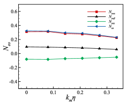
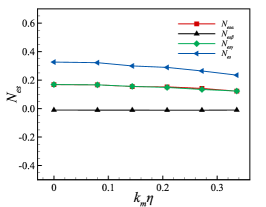
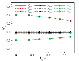
Figure 16: Left: $N_{eo}$ and its components as functions of $k_{m}\eta$. Middle: $N_{es}$ and the contributions $N_{es\alpha}$, $N_{es\beta}$ and $N_{es\gamma}$. Right: the nine components of $N_{es}$. For the cases in group R4.

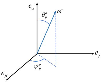
Figure 17: The definitions of $\theta^{o}_{P}$ and $\psi^{o}_{P}$.

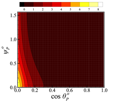
Figure 18: The alignment between ${\bm{\omega}}^{-}$ and the eigenvectors of $s^{+}_{ij}$, for case R$4$K$0$.

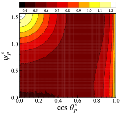
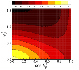
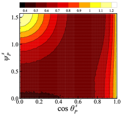
Figure 19: The joint PDFs of $\cos\theta^{s}_{P}$ and $\psi^{s}_{P}$ for ${\bm{e}}^{-}_{\alpha}$ (left) ${\bm{e}}^{-}_{\beta}$ (middle), and ${\bm{e}}^{-}_{\gamma}$ (right). For case R$4$K$0$.

The data for $N_{eo\alpha}$, $N_{eo\beta}$ and $N_{eo\gamma}$ are plotted on the left panel in Fig. 16. The magnitudes of these values decrease only slightly as $k_{m}\eta$ increases. Recalling the normalisation shown in Eq. (57) and the fact that $\langle{\mathcal{D}}_{e}\rangle$ increases as $k_{m}\eta$ increases, the conclusion one may draw is thus that the magnitudes of the non-normalised versions of $N_{eo\alpha}$, $N_{eo\beta}$ and $N_{eo\gamma}$ all increase with $k_{m}\eta$, but at rates that are slightly smaller than that of $\langle{\mathcal{D}}_{e}\rangle$, so that the magnitudes of $N_{eo\alpha}$, $N_{eo\beta}$ and $N_{eo\gamma}$ decrease slightly as $k_{m}\eta$ increases. $N_{eo\beta}$ and $N_{eo\gamma}$ have opposite signs with similar magnitudes. Consequently, $N_{eo}$ is only slightly different from $N_{eo\alpha}$.

$N_{es\alpha}$, $N_{es\beta}$, $N_{es\gamma}$, together with $N_{es}$ are shown in the middle panel of Fig. 16, In terms of the dependence on $k_{m}\eta$, these parameters all behaviour similarly to $N_{eo}$, i.e., their magnitudes all decrease with $k_{m}$, but only weakly. Among the three components, $N_{es\beta}$ is the smallest and essentially negligible. $N_{es\alpha}$ and $N_{es\gamma}$ are both much larger and they appear to be almost the same as each other. The breakdown into the nine components is given in the right panel of Fig. 16. We can see that $N_{es\beta\alpha}$, $N_{es\beta\beta}$, $N_{es\beta\gamma}$, $N_{es\gamma\beta}$, and $N_{es\alpha\beta}$ are all quite small. The largest contributions come from $N_{es\alpha\gamma}$ and $N_{es\gamma\gamma}$, which are positive by definition, and appear to be identical. The contributions from $N_{es\alpha\alpha}$ and $N_{es\gamma\alpha}$ are also significant though somewhat smaller than those from $N_{es\alpha\gamma}$ and $N_{es\gamma\gamma}$. They also appear to be identical.

The results given in the right panel shows that the close agreement between $N_{es\alpha}$ and $N_{es\gamma}$ (middle panel) is a consequence of the close agreement between $N_{es\alpha\ell}$ and $N_{es\gamma\ell}$ ($\ell=\alpha,\beta,\gamma$). The agreement between the latter two is, in fact, a mathematical consequence of the linearity of Eq. (19). The linearity of Eq. (19) dictates that $s^{-}_{ij}$ and $-s^{-}_{ij}$ must have same statistics, which implies that the largest eigenvalues of the two, $\lambda^{-}_{\alpha}$ and $-\lambda^{-}_{\gamma}$, respectively, should have the same statistics too. As a result, $N_{es\alpha\ell}=N_{es\gamma\ell}$ exactly for all $k_{m}$, which is reflected in the figure.

We will not discuss the residual term $r_{e}$ in detail to keep the scope of this investigation manageable. Nevertheless, we may use Eq. (60) to obtain an estimate of its impact by comparing the values of $N_{eo}$ and $N_{es}$ with $2\Lambda$. Recall that, according to the right panel of Fig. 2, $2\Lambda\approx 0.24$ when $k_{m}=0$. On the other hand, Fig. 16 shows that $N_{e}=N_{eo}+N_{es}\approx 0.7$ for $k_{m}=0$. Therefore, the residual term $r_{e}$ has a significant contribution, and appears to be acting to counter the effects of $N_{e}$. Furthermore, $\Lambda$ decreases from $0.12$ to $-0.20$ as $k_{m}\eta$ increases according to Fig. 2 (for cases in group R4). Though $N_{e}$ also decreases with $k_{m}$, the change is not large enough to account for the change in $\Lambda$, which shows that the dependence of $r_{e}$ on $k_{m}$ also plays a role.

Eqs. (63) and (4.3) also suggest that the relative orientations between ${\bm{\omega}}^{-}$ and $s^{+}_{ij}$ or between $s^{-}_{ij}$ and $s^{+}_{ij}$ might impact the values of $N_{eo}$ and $N_{es}$. We thus look into relevant results, for $N_{eo}$ to begin with. The alignment between ${\bm{\omega}}^{-}$ and $s^{+}_{ij}$ can be characterised by the angles $\theta^{o}_{\ell}$ ($\ell=\alpha,\beta,\gamma$) introduced previously. However, since this problem has not been investigated before, we opt for a more complete description based on the polar angle $\theta^{o}_{P}$ and the azimuthal angle $\psi^{o}_{P}$ that the vector ${\bm{\omega}}^{-}$ make in the eigen-frame formed by the eigenvectors of $s^{+}_{ij}$. The definitions of the two angles are illustrated in Fig. 17. Specifically, $\theta^{o}_{P}$ is the angle between ${\bm{\omega}}^{-}$ and the polar direction ${\bm{e}}_{\alpha}$, and $\psi^{o}_{P}$ is the angle between ${\bm{e}}_{\beta}$ and the projection of ${\bm{\omega}}^{-}$ on the equatorial plane. The relations between $(\theta^{o}_{P},\psi^{o}_{P})$ and $\theta^{o}_{i}$ can be derived readily. The joint PDF of $\cos\theta^{o}_{P}$ and $\psi^{o}_{P}$ is shown in Fig. 18. The joint PDF has a very sharp peak at the origin, i.e., at $\theta^{o}_{P}=90^{\circ}$ and $\psi^{o}_{P}=0$. Thus, ${\bm{\omega}}^{-}$ tends to very strongly align with the intermediate eigenvector ${\bm{e}}_{\beta}$ of $s^{+}_{ij}$ (c.f. Fig. 17). This geometrical feature appears to have not be reported before.

The alignment between $s^{+}_{ij}$ and $s^{-}_{ij}$ can be described by the polar angles that each individual eigenvector of $s^{-}_{ij}$ makes in the eigen-frame of $s^{+}_{ij}$. The polar angles are defined in the same way shown in Fig. 17, with ${\bm{\omega}}^{-}$ replaced by one of the eigenvectors, such as ${\bm{e}}^{-}_{\alpha}$. We use $\theta^{s}_{P}$ and $\psi^{s}_{P}$ to denote the angles. Fig. 19 plots the joint PDFs of $\cos\theta^{s}_{P}$ and $\psi^{s}_{P}$ for the three eigenvectors, ${\bm{e}}^{-}_{\alpha}$, ${\bm{e}}^{-}_{\beta}$ and ${\bm{e}}^{-}_{\gamma}$, in the left, middle, and right panels, respectively. Distinct peaks can be identified for all three distributions, though the peaks are not as sharp as in, e.g., Fig. 18. The left panel shows that ${\bm{e}}^{-}_{\alpha}$ displays a bi-modal behaviour, with the alignment switching between $(\theta^{s}_{P},\psi^{s}_{P})=(90^{\circ},90^{\circ})$ and $\theta^{s}_{P}=0^{\circ}$ (the value of $\psi^{s}_{P}$ is not defined when $\theta^{s}_{P}=0$). In the first configuration, ${\bm{e}}^{-}_{\alpha}$ aligns with ${\bm{e}}_{\gamma}$, whereas in the second configuration, ${\bm{e}}^{-}_{\alpha}$ aligns with ${\bm{e}}_{\alpha}$. The eigenvector ${\bm{e}}^{-}_{\beta}$, as shown by the middle panel, tends to align with ${\bm{e}}_{\beta}$, since the PDF peaks at $(\theta^{s}_{P},\psi^{s}_{P})=(90^{\circ},0)$. The right panel shows the joint PDF for ${\bm{e}}^{-}_{\gamma}$. Due to the linearity of the equation for ${\bm{v}}$, it should be exactly the same as the one for ${\bm{e}}^{-}_{\alpha}$ shown in the left panel. Due to statistical fluctuations, the two joint PDFs are not exactly the same, but they are very close, as expected. For example, they display exactly same peak locations.

5 Conclusions

We examine numerically the properties of the Lyapunov exponents and conditional Lyapunov exponent for the Kolmogorov flow in a periodic box. The production and dissipation of the infinitesimal velocity perturbation (i.e., the conditional leading Lyapunov vector) are the focus because they determine the values of the conditional Lyapunov exponents hence the synchronisability of the flow. The study mainly includes two parts, a spectral analysis and a physical space analysis.

In the first part, a detailed analysis of the production spectrum and the dissipation spectrum for the velocity perturbation is conducted. The impacts of the coupling wavenumber are examined. We make several observations: 1) In most cases, the production is positive at all wavenumbers, implying the perturbation is amplified at all scales. 2) Meanwhile, for large coupling wavenumbers, the production spectrum may become negative for some wavenumbers, showing the perturbation at corresponding scales are actually weakened by the production term. 3) The conditional Lyapunov exponents can be smaller than a lower bound proposed recently based on a viscous estimate. 4) The production spectrum is attenuated by coupling and, counter-intuitively, this could amplify the dissipation spectrum for some wavenumbers.

We extend previous discussions on the self-similar evolution of the perturbation spectrum. As a result, a relation required for self-similarity is derived between the local Lyapunov exponent and the integral length scale of the velocity perturbation. The self-similarity of the production spectrum is also examined; we highlight the need for simulations with wider wavenumber range in order to observe clear self-similarity in the production spectrum.

Regarding the peak wavenumber of the perturbation energy spectrum, which has been related to the threshold coupling wavenumber, an analytical relation involving the production spectrum is given. However, to obtain analytical solution for the peak wavenumber, a closure model for the production spectrum is required. We discuss the relation very briefly in a heuristic manner.

With analyses in physical space, we show that the velocity perturbation is stronger in regions in the base flow with strong vorticity or strong straining, but the correlation is weakened when the coupling wavenumber is increased. We employ the transport equation for the dissipation rate of the perturbation to identify two mechanisms that amplify the dissipation: the stretching of perturbation vorticity by the base flow strain rate, and the interaction between the perturbation and base flow strain rates. These observations bring to our attentions the roles of perturbation vorticity and perturbation strain rate that appear to have been neglected previously. The effects of the two mechanisms are then quantified. The geometrical structures of the perturbation vorticity and perturbation strain rate are also discussed.

[Acknowledgement] The authors gratefully acknowledge the anonymous referees for their insightful comments. The explanation for the weakened alignment observed in Fig. 12 is based on the suggestions of one of the referees. Professor K. Yoshida is gratefully acknowledged for providing the data forming part of the right panel of Fig. 2.

[Funding] Jian Li acknowledges the support of the National Natural Science Foundation of China (No. 12102391).

[Data availability statement]The data that support the findings of this study are available from the corresponding author upon reasonable request.

[Declaration of Interests]The authors report no conflict of interest.

References

- Ashurst et al. (1987) Ashurst, Wm.T., Chen, J.-Y. & Rogers, M.M. 1987 Pressure gradient alignment with strain rate and scalar gradient in simulated Navier-Stokes turbulence. Phys. Fluids 30, 3293.
- Boccaletti et al. (2002) Boccaletti, S., Kurths, J., Osipov, G., Valladares, D.L. & Zhou, C.S. 2002 The synchronization of chaotic systems. Phys. Rep. 366, 1–101.
- Boffetta & Musacchio (2017) Boffetta, G. & Musacchio, S. 2017 Chaos and predictability of homogeneous-isotropic turbulence. Phys. Rev. Lett. 119, 054102.
- Buzzicotti & Di Leoni (2020) Buzzicotti, M. & Di Leoni, P.C. 2020 Synchronizing subgrid scale models of turbulence to data. Phys. Fluids 32, 125116.
- Di Leoni et al. (2018) Di Leoni, P.C., Mazzino, A. & Biferale, L. 2018 Inferring flow parameters and turbulent configuration with physics-informed data assimilation and spectral nudging. Phys. Rev. Fluids 3, 104604.
- Di Leoni et al. (2020) Di Leoni, P.C., Mazzino, A. & Biferale, L. 2020 Synchronization to big data: Nudging the Navier-Stokes equations for data assimilation of turbulent flows. Phys. Rev. X 10, 011023.
- Fujisaka & Yamada (1983) Fujisaka, H. & Yamada, T. 1983 Stability theory of synchronized motion in coupled-oscillator systems. Prog. Theor. Phys. 69, 32.
- Ge et al. (2023) Ge, J., Rolland, J. & Vassilicos, J.C. 2023 The production of uncertainty in three-dimensional Navier-Stokes turbulence. J. Fluid Mech. 977, A17.
- Henshaw et al. (2003) Henshaw, W.D., Kreiss, H.-O. & Ystróm, J. 2003 Numerical experiments on the interaction between the large- and small-scale motions of the Navier-Stokes equations. Multiscale Model. Simul. 1, 119–149.
- Inubushi et al. (2023) Inubushi, M., Saiki, Y., Kobayashi, M.U. & Goto, S. 2023 Characterizing small-scale dynamics of Navier-Stokes turbulence with transverse Lyapunov exponents: A data assimilation approach. Phys. Rev. Lett. 131 (25), 254001.
- Lalescu et al. (2013) Lalescu, C.C., Meneveau, C. & Eyink, G.L. 2013 Synchronization of chaos in fully developed turbulence. Phys. Rev. Lett. 110, 084102.
- Li et al. (2024a) Li, J., Si, W., Li, Y. & Xu, P. 2024a Intrinsic relationship between synchronisation thresholds and Lyapunov vectors: evidence from large eddy simulations and shell models, arXiv: 2407.13081v2.
- Li et al. (2022) Li, J., Tian, M. & Li, Y. 2022 Synchronizing large eddy simulations with direct numerical simulations via data assimilation. Phys. Fluids 34, 065108.
- Li et al. (2024b) Li, J., Tian, M., Li, Y., Si, W. & Mohammed, H.K. 2024b The conditional Lyapunov exponents and synchronisation of rotating turbulent flows. J. Fluid Mech. 983, A1.
- Meneveau (2011) Meneveau, C. 2011 Lagrangian dynamics and models of the velocity gradient tensor in turbulent flows. Ann. Rev. Fluid Mech. 43, 219–245.
- Nikitin (2008) Nikitin, N. 2008 On the rate of spatial predictability in near-wall turbulence. J. Fluid Mech. 614, 495–507.
- Nikitin (2018) Nikitin, N. 2018 Characteristics of the leading Lyapunov vector in a turbulent channel flow. J. Fluid Mech. 849, 942–967.
- Nikolaidis & Ioannou (2022) Nikolaidis, M.-A. & Ioannou, P. J. 2022 Synchronization of low Reynolds number plane Couette turbulence. J. Fluid Mech. 933.
- Olson & Titi (2003) Olson, E. & Titi, E. S. 2003 Determining modes for continuous data assimilation in 2D turbulence. Journal of Statistical Physics 113, 799–840.
- Pope (2000) Pope, S. B. 2000 Turbulent flows. Cambridge University Press, Cambridge.
- Vela-Martin (2021) Vela-Martin, A. 2021 The synchronisation of intense vorticity in isotropic turbulence. J. Fluid Mech. 913, R8.
- Wang & Zaki (2022) Wang, M. & Zaki, T. A. 2022 Synchronization of turbulence in channel flow. J. Fluid Mech. 943, A4.
- Wang et al. (2023) Wang, Y, Yuan, Z & Wang, J 2023 A further investigation on the data assimilation-based small-scale reconstruction of turbulence. Phys. Fluids 35 (1), 015143.
- Wang et al. (2022) Wang, Y., Yuan, Z., Xie, C. & Wang, J. 2022 Temporally sparse data assimilation for the small-scale reconstruction of turbulence. Phys. Fluids 34 (6), 065115.
- Yoshida et al. (2005) Yoshida, K., Yamaguchi, J. & Kaneda, Y. 2005 Regeneration of small eddies by data assimilation in turbulence. Phys. Rev. Lett. 94, 014501.
- Yoshimatsu & Ariki (2019) Yoshimatsu, K. & Ariki, T. 2019 Error growth in three-dimensional homogeneous turbulence. J. Phys. Soc. Jpn. 88, 124401.