Supplemental Material: Synthetic Gauge Field for Ultracold Atoms Induced by Vector Beams

In this Supplemental Material (SM), we provide further details on the explicit expressions of electric fields of the tightly focused vector beams (VBs), the detailed energy level configuration, the derivation of the Hamiltonians for the single-particle and weakly interacting cases, the VB-indudced potentials for varying VB paramters, and the analysis of spin textures.

S-1 Electric fields of tightly focused vector beams

We introduce the electric fields of tightly focused VBs after passing through a high-numerical-aperture (NA) lens, as shown in Fig. 1 of the main text. The electric field at the focal plane are determined using Richards-Wolf vectorial diffraction integral [1, 2, 3] in the cylindrical coordinates $(\rho,\varphi,z)$, given by:

$$E_{x} =\mathrm{i}^{a+1}\cos(\alpha/2)\mathrm{e}^{-\mathrm{i}\beta/2}\Big{[}\mathrm{e}^{\mathrm{i}a\varphi}\mathcal{I}_{a}+\mathrm{e}^{\mathrm{i}(a+2)\varphi}\mathcal{I}^{\prime\prime}_{a+2}\Big{]}+\mathrm{i}^{b+1}\sin(\alpha/2)\mathrm{e}^{\mathrm{i}\beta/2}\Big{[}\mathrm{e}^{\mathrm{i}b\varphi}\mathcal{I}_{b}+\mathrm{e}^{\mathrm{i}(b-2)\varphi}\mathcal{I}^{\prime\prime}_{b-2}\Big{]},$$ (S1)

$$E_{y} =\mathrm{i}^{a+2}\cos(\alpha/2)\mathrm{e}^{-\mathrm{i}\beta/2}\Big{[}\mathrm{e}^{\mathrm{i}a\varphi}\mathcal{I}_{a}-\mathrm{e}^{\mathrm{i}(a+2)\varphi}\mathcal{I}^{\prime\prime}_{a+2}\Big{]}+\mathrm{i}^{b}\sin(\alpha/2)\mathrm{e}^{\mathrm{i}\beta/2}\Big{[}\mathrm{e}^{\mathrm{i}b\varphi}\mathcal{I}_{b}-\mathrm{e}^{\mathrm{i}(b-2)\varphi}\mathcal{I}^{\prime\prime}_{b-2}\Big{]},$$ (S2)

$$E_{z} =-\mathrm{i}^{a+2}\cos(\alpha/2)\mathrm{e}^{-\mathrm{i}\beta/2}\mathrm{e}^{\mathrm{i}(a+1)\varphi}\mathcal{I}^{\prime}_{a+1}-\mathrm{i}^{b}\sin(\alpha/2)\mathrm{e}^{\mathrm{i}\beta/2}\mathrm{e}^{\mathrm{i}(b-1)\varphi}\mathcal{I}^{\prime}_{b-1},$$ (S3)

where $a\equiv l-m$, and $b\equiv l+m$. $\alpha$ and $\beta$ are spherical coordinates of high-order Poincaré sphere as shown in Fig. 1 (b). $\mathcal{I}_{n}$, $\mathcal{I}^{\prime}_{n}$, and $\mathcal{I}^{\prime\prime}_{n}$ depend on spatial coordinates $\rho$ and $z$, expressed as

$$\mathcal{I}_{n} =-kF\int_{0}^{\theta_{\max}}\mathrm{d}\theta~\bar{A}_{l}(\theta)\sin\theta\cos^{1/2}(\theta)(1+\cos\theta)e^{\mathrm{i}kz\cos\theta}J_{n}(k\rho\sin\theta),$$ (S4)

$$\mathcal{I}^{\prime}_{n} =-2kF\int_{0}^{\theta_{\max}}\mathrm{d}\theta~\bar{A}_{l}(\theta)\sin^{2}\theta\cos^{1/2}(\theta)e^{\mathrm{i}kz\cos\theta}J_{n}(k\rho\sin\theta),$$ (S5)

$$\mathcal{I}^{\prime\prime}_{n} =-kF\int_{0}^{\theta_{\max}}\mathrm{d}\theta~\bar{A}_{l}(\theta)\sin\theta\cos^{1/2}(\theta)(1-\cos\theta)e^{\mathrm{i}kz\cos\theta}J_{n}(k\rho\sin\theta),$$ (S6)

where $k=2\pi/\lambda$ is the the wave number, $\lambda$ is the wavelength, and $J_{n}(x)$ denotes the $n$-th order Bessel function of the first kind. The angle $\theta$ is defined for the point $(\rho,\varphi,z=-F)$ on the plane where the high-NA lens (with focal length $F$) is located, such that $\sin\theta=\rho/F$ and $0\leq\theta\leq\theta_{\text{max}}$ with $\sin\theta_{\text{max}}=\mathrm{NA}$. The amplitude profile $\bar{A}_{l}(\theta)$ is given by

$$\bar{A}_{l}(\theta)=\sqrt{I}\left[\frac{\sqrt{2}\zeta\sin(\theta)}{\sin(\theta_{\max})}\right]^{|l|}\exp\left[-\zeta^{2}\left(\frac{\sin(\theta)}{\sin(\theta_{\max})}\right)^{2}\right],$$ (S7)

where $\zeta=F\sin(\theta_{\max})/w$ . In this work, we use a high-NA lens with $\mathrm{NA}=0.8$, $F=1.95\mathrm{mm}$, and set $\zeta=8$ (or $w=0.195\mathrm{mm}$).

S-2 Single-particle Hamiltonian

We consider $N=1000$ ⁸⁷Rb atoms trapped in an optical dipole trap with trapping frequencies $\omega_{x}=\omega_{y}=\omega=2\pi\times 103.3\mathrm{Hz}$ and $\omega_{z}=10\omega$, and transverse trap size $a_{0}\approx 1.06\mathrm{\mu m}$. The system includes Zeeman sublevels $\left|\downarrow\right\rangle\equiv\left|5^{2}S_{1/2},F=1,m_{F}=0\right\rangle$ and $\left|\uparrow\right\rangle\equiv\left|5^{2}S_{1/2},F=1,m_{F}=-1\right\rangle$, and the excited states $|5^{2}P_{1/2},F=1,m_{F}=0\rangle$ and $|5^{2}P_{1/2},F=1,m_{F}=-1\rangle$, forming a double-$\Lambda$-type energy level configuration as shown in Fig. S1 and Fig. 1 (c) of the main text. The states $\left|\uparrow\right\rangle$ and $\left|\downarrow\right\rangle$ are coupled via two-photon Raman processes, obeying the selection rules for the $\sigma_{1}^{+}$ and $\pi_{2}$ components, or the $\pi_{1}$ and $\sigma_{2}^{-}$ components of the tightly focused VBs.

Figure S1: Double-$\Lambda$-type energy level configuration. Optical transitions allowed by the selection rules involve the $\sigma_{1}^{+}$ and $\pi_{2}$ components or the $\pi_{1}$ and $\sigma_{2}^{-}$ components of the tightly focused VBs with optical frequencies $\omega_{1}$ (red) and $\omega_{2}$ (blue).

The single-particle Hamiltonian is given by

$$H_{0}=-\frac{\hbar^{2}\nabla^{2}}{2M}+\frac{1}{2}M\omega^{2}\rho^{2}+\frac{1}{2}M\omega_{z}^{2}z^{2}+h_{\mathrm{eff}},$$ (S8)

where $h_{\mathrm{eff}}$ is the effective Hamiltonian for atoms in the ground-state manifold during the Raman process, expressed as [4, 5, 6, 7]

$$h_{\mathrm{eff}}=u_{s}|\tilde{\mathbf{E}}|^{2}+\frac{\mu_{B}g_{F}}{\hbar}\left(\mathbf{B}+\mathbf{B}_{\mathrm{eff}}\right)\cdot\mathbf{F}.$$ (S9)

The first term represents the scalar light shift, while the second term contains the effective magnetic field

$$\mathbf{B}_{\mathrm{eff}}=\frac{\mathrm{i}u_{v}(\tilde{\mathbf{E}}^{*}\times\tilde{\mathbf{E}})}{\mu_{B}g_{J}},$$ (S10)

which is generated by the vector light shift. $u_{s}$ and $u_{v}$ are the scalar and vector polarizabilities, respectively [4, 5, 6, 7]. The vector light shift induces coupling between different spin states. In our scheme, the total electric field experienced by the atoms is given by

$$\tilde{\mathbf{E}}=\mathbf{E}_{1}\mathrm{e}^{\mathrm{i}\omega_{1}t}+\mathbf{E}_{2}\mathrm{e}^{\mathrm{i}\omega_{2}t},$$ (S11)

where $\mathbf{E}_{1}=(E_{x1},E_{y1},E_{z1})$ and $\mathbf{E}_{2}=(E_{x2},E_{y2},E_{z2})$. We find the potential induced by scalar light shift

$$V_{\mathrm{S}}(\mathbf{r})=u_{s}(\mathbf{E}_{1}^{*}\cdot\mathbf{E}_{1}+\mathbf{E}_{2}^{*}\cdot\mathbf{E}_{2}),$$ (S12)

and the effective potential $\mathbf{B}_{\mathrm{eff}}=(B_{x},B_{y},B_{z})$ has components

$$B_{x} =\frac{\mathrm{i}u_{v}}{\mu_{B}g_{J}}\biggl{[}(E_{y1}^{*}E_{z2}-E_{z1}^{*}E_{y2})\mathrm{e}^{-\mathrm{i}(\omega_{1}-\omega_{2})t}+(E_{y2}^{*}E_{z1}-E_{z2}^{*}E_{y1})\mathrm{e}^{\mathrm{i}(\omega_{1}-\omega_{2})t}\biggr{]},$$

$$B_{y} =\frac{\mathrm{i}u_{v}}{\mu_{B}g_{J}}\biggl{[}(E_{z1}^{*}E_{x2}-E_{x1}^{*}E_{z2})\mathrm{e}^{-\mathrm{i}(\omega_{1}-\omega_{2})t}+(E_{z2}^{*}E_{x1}-E_{x2}^{*}E_{z1})\mathrm{e}^{\mathrm{i}(\omega_{1}-\omega_{2})t}\biggr{]},$$

$$B_{z} =\frac{\mathrm{i}u_{v}}{\mu_{B}g_{J}}(E_{x1}^{*}E_{y1}-E_{y1}^{*}E_{x1}+E_{x2}^{*}E_{y2}-E_{y2}^{*}E_{x2}).$$ (S13)

Here we have neglected the terms corresponding to the forbidden optical transitions.

The effective Hamiltonian is reduced to [5, 6, 7]

$$h_{\mathrm{eff}}=V_{\mathrm{S}}(\mathbf{r})+\frac{\mu_{B}g_{F}}{2}(B_{z}\sigma_{z}+B_{x}\sigma_{x}+B_{y}\sigma_{y}).$$ (S14)

After performing the rotating wave approximation and a unitary transformation with $U=e^{\mathrm{i}(\omega_{1}-\omega_{2})t\hat{\sigma}_{z}/2}$, the single-particle Hamiltonian becomes

$$H_{0}=-\frac{\hbar^{2}\nabla^{2}}{2M}+\frac{1}{2}M\omega^{2}\rho^{2}+\frac{1}{2}M\omega_{z}^{2}z^{2}+V_{\mathrm{S}}(\mathbf{r})+\frac{\delta}{2}\sigma_{z}+\begin{pmatrix}\Omega_{z}(\mathbf{r})&\Omega_{r}(\mathbf{r})\\ \Omega_{r}^{*}(\mathbf{r})&-\Omega_{z}(\mathbf{r})\end{pmatrix},$$ (S15)

where

$$V_{\mathrm{S}}(\mathbf{r}) =\Omega_{s}(\mathbf{\bar{E}}_{1}^{*}\cdot\mathbf{\bar{E}}_{1}+\mathbf{\bar{E}}_{2}^{*}\cdot\mathbf{\bar{E}}_{2}),$$ (S16)

$$\Omega_{z}(\mathbf{r}) =\Omega_{0}\mathrm{i}(\bar{E}_{x1}^{*}\bar{E}_{y1}-\bar{E}_{y1}^{*}\bar{E}_{x1}+\bar{E}_{x2}^{*}\bar{E}_{y2}-\bar{E}_{y2}^{*}\bar{E}_{x2}),$$ (S17)

$$\Omega_{r}(\mathbf{r}) =\Omega_{0}\big{[}(\bar{E}_{z2}^{*}\bar{E}_{x1}-\bar{E}_{x2}^{*}\bar{E}_{z1})+\mathrm{i}(\bar{E}_{y2}^{*}\bar{E}_{z1}-\bar{E}_{z2}^{*}\bar{E}_{y1})\big{]},$$ (S18)

and the coupling strengths are

$$\Omega_{s} =u_{s}(I_{1}+I_{2}),$$ (S19)

$$\Omega_{0} =\frac{u_{v}g_{F}\sqrt{I_{1}I_{2}}}{2g_{J}}.$$ (S20)

Here $I_{1}$ and $I_{2}$ are the light intensities of the two VBs, and $\mathbf{\bar{E}}_{j}=\mathbf{E}_{j}/\sqrt{I_{j}}=(\bar{E}_{xj},\bar{E}_{yj},\bar{E}_{zj})$ is the normalized electric fields. When interatomic interactions are weak, the motion of atoms can be approximated as a two-dimensional problem [8, 9, 10, 11]. We focus on the physics near the focal plane at $z=0$, and the potentials approximately reduce to $V_{\mathrm{S}}(\mathbf{r})=V_{\mathrm{S}}(\bm{\rho})$, $\Omega_{z}(\mathbf{r})=\Omega_{z}(\bm{\rho})$, and $\Omega_{r}(\mathbf{r})=\Omega_{r}(\bm{\rho})$.

In the main text, for the angular stripe phase in Fig. 2, we adopt a wavelength of $\lambda=797\mathrm{nm}$. $\Omega_{s}$ is set to be finite and negative, inducing annular confinement via $V_{\mathrm{S}}(\bm{\rho})$. We find the ratio $\Omega_{0}/\Omega_{s}=-\frac{u_{v}\sqrt{I_{1}I_{2}}}{8u_{s}(I_{1}+I_{2})}$, and $u_{v}/u_{s}\approx 1.42$ for $\lambda=797\mathrm{nm}$ [4]. Given $\Omega_{s}$, $\Omega_{0}$ can be tuned by adjusting the intensities $I_{1}$ and $I_{2}$ of the VBs, making the angular stripe phase experimentally accessible. In Fig. 3 of the main text, we adopt the tune-out wavelength $\lambda=790\mathrm{nm}$, where the scalar polarizability vanishes, so $\Omega_{s}\approx 0$. Here the coupling strength $\Omega_{0}$ is also tunable by adjusting two VBs’ light intensities.

S-3 Weakly interacting condensate

We now consider the weakly interacting case. The Gross-Pitaevskii (GP) equation is given by

$$\mathrm{i}\hbar\frac{\partial}{\partial t}\Psi^{\mathrm{3D}}=(H_{0}+V_{\mathrm{I}})\Psi^{3\mathrm{D}},$$ (S21)

where $V_{\mathrm{I}}$ represents the mean-field interaction:

$$V_{\mathrm{I}}(\mathbf{r})=\begin{pmatrix}g_{\uparrow\uparrow}|\psi^{\mathrm{3D}}_{\uparrow}(\mathbf{r})|^{2}+g_{\uparrow\downarrow}|\psi^{\mathrm{3D}}_{\downarrow}(\mathbf{r})|^{2}&0\\ 0&g_{\uparrow\downarrow}|\psi^{\mathrm{3D}}_{\uparrow}(\mathbf{r})|^{2}+g_{\downarrow\downarrow}|\psi^{\mathrm{3D}}_{\downarrow}(\mathbf{r})|^{2}\end{pmatrix}.$$ (S22)

Here $g_{\sigma\sigma^{\prime}}=4\pi\hbar^{2}Na_{\sigma\sigma^{\prime}}^{s}/M$ is the nonlinear interaction strength, $a_{\sigma\sigma^{\prime}}^{s}$ is the s-wave scattering length between two spins $\sigma=\uparrow,\downarrow$, and $N$ is total number of atoms.

In our scheme, we consider a pancake-shaped Bose-Einstein condensate (BEC) with the trapping frequency $\omega_{z}\gg\omega$. The wave function is approximated as

$$\Psi^{\mathrm{3D}}=\begin{pmatrix}\psi_{\uparrow}(\bm{\rho})\\ \psi_{\downarrow}(\bm{\rho})\end{pmatrix}\psi^{\mathrm{1D}}(z).$$ (S23)

Inserting Eqs. (S15), (S22) and (S23) into the GP equation, and integrating both sides with respect to $z$ [9], we obtain

$$\mathrm{i}\hbar\frac{\partial\psi_{\uparrow}}{\partial t} =\left[-\frac{\hbar^{2}\nabla_{\rho}^{2}}{2M}+\frac{1}{2}M\omega^{2}{\rho}^{2}+V_{\mathrm{S}}(\bm{\rho})+\frac{\delta}{2}+\Omega_{z}(\bm{\rho})+\eta\left(g_{\uparrow\uparrow}\left|\psi_{\uparrow}\right|^{2}+g_{\uparrow\downarrow}\left|\psi_{\downarrow}\right|^{2}\right)\right]\psi_{\uparrow}+C\psi_{\uparrow}+\Omega_{r}(\bm{\rho})\psi_{\downarrow},$$ (S24)

$$\mathrm{i}\hbar\frac{\partial\psi_{\downarrow}}{\partial t} =\left[-\frac{\hbar^{2}\nabla_{\rho}^{2}}{2M}+\frac{1}{2}M\omega^{2}{\rho}^{2}+V_{\mathrm{S}}(\bm{\rho})-\frac{\delta}{2}-\Omega_{z}(\bm{\rho})+\eta\left(g_{\uparrow\downarrow}\left|\psi_{\uparrow}\right|^{2}+g_{\downarrow\downarrow}\left|\psi_{\downarrow}\right|^{2}\right)\right]\psi_{\downarrow}+C\psi_{\downarrow}+\Omega_{r}^{\ast}(\bm{\rho})\psi_{\uparrow}.$$ (S25)

Here the constant $C$ and the dimensional reduction factor $\eta$ are defined as

$$\eta=\frac{\int_{z}\left|\psi^{\mathrm{1D}}(z)\right|^{4}dz}{\int_{z}\left|\psi^{\mathrm{1D}}(z)\right|^{2}dz},\qquad C=\frac{\hbar^{2}}{2M}\frac{\int_{z}\left|\frac{d\psi^{\mathrm{1D}}(z)}{dz}\right|^{2}dz}{\int_{z}\left|\psi^{\mathrm{1D}}(z)\right|^{2}dz}+\frac{1}{2}M\omega_{z}^{2}\frac{\int_{z}z^{2}\left|\psi^{\mathrm{1D}}(z)\right|^{2}dz}{\int_{z}\left|\psi^{\mathrm{1D}}(z)\right|^{2}dz}.$$ (S26)

Substituting $\psi_{\sigma}=\exp(-\mathrm{i}Ct/\hbar)\tilde{\psi}_{\sigma}$, and replacing $\tilde{\psi}_{\sigma}\rightarrow\psi_{\sigma}$, we obtain the reduced two-dimensional GP equation

$$\mathrm{i}\hbar\frac{\partial\psi_{\uparrow}}{\partial t} =\left[-\frac{\hbar^{2}\nabla_{\rho}^{2}}{2M}+\frac{1}{2}M\omega^{2}{\rho}^{2}+V_{\mathrm{S}}(\bm{\rho})+\frac{\delta}{2}+\Omega_{z}(\bm{\rho})+\eta\left(g_{\uparrow\uparrow}\left|\psi_{\uparrow}\right|^{2}+g_{\uparrow\downarrow}\left|\psi_{\downarrow}\right|^{2}\right)\right]\psi_{\uparrow}+\Omega_{r}(\bm{\rho})\psi_{\downarrow},$$ (S27)

$$\mathrm{i}\hbar\frac{\partial\psi_{\downarrow}}{\partial t} =\left[-\frac{\hbar^{2}\nabla_{\rho}^{2}}{2M}+\frac{1}{2}M\omega^{2}{\rho}^{2}+V_{\mathrm{S}}(\bm{\rho})-\frac{\delta}{2}-\Omega_{z}(\bm{\rho})+\eta\left(g_{\uparrow\downarrow}\left|\psi_{\uparrow}\right|^{2}+g_{\downarrow\downarrow}\left|\psi_{\downarrow}\right|^{2}\right)\right]\psi_{\downarrow}+\Omega_{r}^{\ast}(\bm{\rho})\psi_{\uparrow}.$$ (S28)

Moreover, the 1D wave function $\psi^{\mathrm{1D}}(z)$ is given by form [12]

$$\psi^{\mathrm{1D}}(z)=\frac{\mathrm{e}^{-z^{2}/2a_{0z}^{2}}}{\pi^{1/4}a_{0z}^{1/2}},$$ (S29)

where $a_{0z}\equiv\sqrt{\hbar/M\omega_{z}}$ is the trap size along the $z$-axis. Therefore, the dimensional reduction factor is $\eta=1/(\sqrt{2\pi}a_{0z})$.

S-4 The forms of $\Omega_{r}$ and $\Omega_{z}$ for varying VB parameters

To analytically demonstrate the forms of $\Omega_{r}(\bm{\rho})$ and $\Omega_{z}(\bm{\rho})$, we substitute the electric fields from Eqs. (S1)-(S3) into the last term of Eq. (S15). For simplicity, assuming both VBs have the same orientation angle $\beta_{1}=\beta_{2}=0$, we obtain

$$\Omega_{r}(\bm{\rho}) =f_{r}^{1}(\rho)\Theta_{r}^{1}(\alpha_{1},\alpha_{2})e^{\mathrm{i}\bar{l}_{1}\varphi}+f_{r}^{2}(\rho)\Theta_{r}^{2}(\alpha_{1},\alpha_{2})e^{\mathrm{i}\bar{l}_{2}\varphi}+f_{r}^{3}(\rho)\Theta_{r}^{3}(\alpha_{1},\alpha_{2})e^{\mathrm{i}\bar{l}_{3}\varphi}+f_{r}^{4}(\rho)\Theta_{r}^{4}(\alpha_{1},\alpha_{2})e^{\mathrm{i}\bar{l}_{4}\varphi},$$ (S30)

$$\Omega_{z}(\bm{\rho}) =f_{z}^{1}(\rho)\Theta_{z}^{1}(\alpha_{1})+f_{z}^{2}(\rho)\Theta_{z}^{2}(\alpha_{2})+f_{z}^{3}(\rho)\Theta_{z}^{3}(\alpha_{1})+f_{z}^{4}(\rho)\Theta_{z}^{4}(\alpha_{2})$$

$$+f_{z}^{5}(\rho)\Theta_{z}^{5}(\alpha_{1})e^{\mathrm{i}\overline{l}_{5}\varphi}+f_{z}^{6}(\rho)\Theta_{z}^{6}(\alpha_{1})e^{-\mathrm{i}\overline{l}_{5}\varphi}+f_{z}^{7}(\rho)\Theta_{z}^{7}(\alpha_{2})e^{\mathrm{i}\overline{l}_{6}\varphi}+f_{z}^{8}(\rho)\Theta_{z}^{8}(\alpha_{2})e^{-\mathrm{i}\overline{l}_{6}\varphi},$$ (S31)

with

$$f_{r}^{1}(\rho) =2\mathrm{i}^{a_{1}+1}(-\mathrm{i})^{a_{2}}(\mathcal{I}_{a_{1}}\mathcal{I}^{\prime}_{a_{2}+1}+\mathcal{I}^{\prime}_{a_{1}+1}\mathcal{I}^{\prime\prime}_{a_{2}+2}),\quad \Theta_{r}^{1}(\alpha_{1},\alpha_{2}) =\cos(\alpha_{1}/2)\cos(\alpha_{2}/2),$$

$$f_{r}^{2}(\rho) =2\mathrm{i}^{a_{1}+1}(-\mathrm{i})^{b_{2}}(\mathcal{I}^{\prime}_{a_{1}+1}\mathcal{I}_{b_{2}}-\mathcal{I}_{a_{1}}\mathcal{I}^{\prime}_{b_{2}-1}),\quad \Theta_{r}^{2}(\alpha_{1},\alpha_{2}) =\cos(\alpha_{1}/2)\sin(\alpha_{2}/2),$$

$$f_{r}^{3}(\rho) =2\mathrm{i}^{b_{1}+1}(-\mathrm{i})^{a_{2}}(\mathcal{I}^{\prime\prime}_{b_{1}-2}\mathcal{I}^{\prime}_{a_{2}+1}-\mathcal{I}^{\prime}_{b_{1}-1}\mathcal{I}^{\prime\prime}_{a_{2}+2}),\quad \Theta_{r}^{3}(\alpha_{1},\alpha_{2}) =\sin(\alpha_{1}/2)\cos(\alpha_{2}/2),$$

$$f_{r}^{4}(\rho) =-2\mathrm{i}^{b_{1}+1}(-\mathrm{i})^{b_{2}}(\mathcal{I}^{\prime}_{b_{1}-1}\mathcal{I}_{b_{2}}+\mathcal{I}^{\prime\prime}_{b_{1}-2}\mathcal{I}^{\prime}_{b_{2}-1}),\quad \Theta_{r}^{4}(\alpha_{1},\alpha_{2}) =\sin(\alpha_{1}/2)\sin(\alpha_{2}/2),$$

$$f_{z}^{1}(\rho) =-2(\mathcal{I}_{a_{1}}^{2}-\mathcal{I}_{a_{1}+2}^{\prime\prime 2}),\quad \Theta_{z}^{1}(\alpha_{1}) =\cos^{2}(\alpha_{1}/2),$$

$$f_{z}^{2}(\rho) =-2(\mathcal{I}_{a_{2}}^{2}-\mathcal{I}_{a_{2}+2}^{\prime\prime 2}),\quad \Theta_{z}^{2}(\alpha_{2}) =\cos^{2}(\alpha_{2}/2),$$

$$f_{z}^{3}(\rho) =2(\mathcal{I}_{b_{1}}^{2}-\mathcal{I}_{b_{1}-2}^{\prime\prime 2}),\quad \Theta_{z}^{3}(\alpha_{1}) =\sin^{2}(\alpha_{1}/2),$$

$$f_{z}^{4}(\rho) =2(\mathcal{I}_{b_{2}}^{2}-\mathcal{I}_{b_{2}-2}^{\prime\prime 2}),\quad \Theta_{z}^{4}(\alpha_{2}) =\sin^{2}(\alpha_{2}/2),$$

$$f_{z}^{5}(\rho) =(-\mathrm{i})^{b_{1}}\mathrm{i}^{a_{1}}(\mathcal{I}^{\prime\prime}_{a_{1}+2}\mathcal{I}_{b_{1}}-\mathcal{I}_{a_{1}}\mathcal{I}^{\prime\prime}_{b_{1}-2}),\quad \Theta_{z}^{5}(\alpha_{1}) =\sin(\alpha_{1}),$$

$$f_{z}^{6}(\rho) =(-\mathrm{i})^{a_{1}}\mathrm{i}^{b_{1}}(\mathcal{I}^{\prime\prime}_{a_{1}+2}\mathcal{I}_{b_{1}}-\mathcal{I}_{a_{1}}\mathcal{I}^{\prime\prime}_{b_{1}-2}),\quad \Theta_{z}^{6}(\alpha_{1}) =\sin(\alpha_{1}),$$

$$f_{z}^{7}(\rho) =(-\mathrm{i})^{b_{2}}\mathrm{i}^{a_{2}}(\mathcal{I}^{\prime\prime}_{a_{2}+2}\mathcal{I}_{b_{2}}-\mathcal{I}_{a_{2}}\mathcal{I}^{\prime\prime}_{b_{2}-2}),\quad \Theta_{z}^{7}(\alpha_{2}) =\sin(\alpha_{2}),$$

$$f_{z}^{8}(\rho) =(-\mathrm{i})^{a_{2}}\mathrm{i}^{b_{2}}(\mathcal{I}^{\prime\prime}_{a_{2}+2}\mathcal{I}_{b_{2}}-\mathcal{I}_{a_{2}}\mathcal{I}^{\prime\prime}_{b_{2}-2}),\quad \Theta_{z}^{8}(\alpha_{2}) =\sin(\alpha_{2}).$$

The $f$-functions with subscript $r$ only depend on the spatial variable $\rho$. Here $a_{j}=l_{j}-m_{j}$ and $b_{j}=l_{j}+m_{j}$ with $j=1,2$. $\alpha_{1}$ and $\alpha_{2}$ denote the ellipticity angles on the high-order Poincaré sphere. We define the effective topological charges as:

$$\bar{l}_{1} =l_{1}-l_{2}-m_{1}+m_{2}-1,$$

$$\bar{l}_{2} =l_{1}-l_{2}-m_{1}-m_{2}+1,$$

$$\bar{l}_{3} =l_{1}-l_{2}+m_{1}+m_{2}-3,$$

$$\bar{l}_{4} =l_{1}-l_{2}+m_{1}-m_{2}-1,$$

$$\bar{l}_{5} =2-2m_{1},$$

$$\bar{l}_{6} =2-2m_{2}.$$ (S32)

By varying the VB parameters $(l_{j},m_{j},\alpha_{j},\beta_{j})$ with $j=1,2$, we can adjust the forms of $\Omega_{r}(\bm{\rho})$ and $\Omega_{z}(\bm{\rho})$, leading to different potentials for the atoms. The specific forms of $\Omega_{r}(\bm{\rho})$ and $\Omega_{z}(\bm{\rho})$ for various VB parameters are presented in Table S1.

Table S1: $\Omega_{r}$ and $\Omega_{z}$ for different sets of VB parameters

Scenario	$\Omega_{r}/\Omega_{0}$	$\Omega_{z}/\Omega_{0}$	note
1. $\alpha_{1}=0,\alpha_{2}=0$	$f_{r}^{1}e^{\mathrm{i}\bar{l}\varphi}$	$f_{z}^{1}+f_{z}^{2}$	$\bar{l}=\bar{l}_{1}$
2. $\alpha_{1}=0,\alpha_{2}=\pi$	$f_{r}^{2}e^{\mathrm{i}\bar{l}\varphi}$	$f_{z}^{1}+f_{z}^{2}$	$\bar{l}=\bar{l}_{2}$
3. $\alpha_{1}=\pi,\alpha_{2}=0$	$f_{r}^{3}e^{\mathrm{i}\bar{l}\varphi}$	$f_{z}^{3}+f_{z}^{4}$	$\bar{l}=\bar{l}_{3}$
4. $\alpha_{1}=\pi,\alpha_{2}=\pi$	$f_{r}^{4}e^{\mathrm{i}\bar{l}\varphi}$	$f_{z}^{3}+f_{z}^{4}$	$\bar{l}=\bar{l}_{4}$
5. $\alpha_{1}=0,\alpha_{2}=\forall$	$[f_{r}^{1}\Theta_{r}^{1}+f_{r}^{2}\Theta_{r}^{2}]e^{\mathrm{i}\bar{l}\varphi}$	$f_{z}^{1}+f_{z}^{2}\Theta_{z}^{2}+f_{z}^{4}\Theta_{z}^{4}$	$\bar{l}=\bar{l}_{1}=\bar{l}_{2}$
$Cond:m_{2}=1$		$+f_{z}^{7}\Theta_{z}^{7}+f_{z}^{8}\Theta_{z}^{8}$
6. $\alpha_{1}=\pi,\alpha_{2}=\forall$	$[f_{r}^{3}\Theta_{r}^{3}+f_{r}^{4}\Theta_{r}^{4}]e^{\mathrm{i}\bar{l}\varphi}$	$f_{z}^{3}+f_{z}^{2}\Theta_{z}^{2}+f_{z}^{4}\Theta_{z}^{4}$	$\bar{l}=\bar{l}_{3}=\bar{l}_{4}$
$Cond:m_{2}=1$		$+f_{z}^{7}\Theta_{z}^{7}+f_{z}^{8}\Theta_{z}^{8}$
7. $\alpha_{1}=\forall,\alpha_{2}=0$	$[f_{r}^{1}\Theta_{r}^{1}+f_{r}^{3}\Theta_{r}^{3}]e^{\mathrm{i}\bar{l}\varphi}$	$f_{z}^{2}+f_{z}^{1}\Theta_{z}^{1}+f_{z}^{3}\Theta_{z}^{3}$	$\bar{l}=\bar{l}_{1}=\bar{l}_{3}$
$Cond:m_{1}=1$		$+f_{z}^{5}\Theta_{z}^{5}+f_{z}^{6}\Theta_{z}^{6}$
8. $\alpha_{1}=\forall,\alpha_{2}=\pi$	$[f_{r}^{2}\Theta_{r}^{2}+f_{r}^{4}\Theta_{r}^{4}]e^{\mathrm{i}\bar{l}\varphi}$	$f_{z}^{4}+f_{z}^{1}\Theta_{z}^{1}+f_{z}^{3}\Theta_{z}^{3}$	$\bar{l}=\bar{l}_{2}=\bar{l}_{4}$
$Cond:m_{1}=1$		$+f_{z}^{5}\Theta_{z}^{5}+f_{z}^{6}\Theta_{z}^{6}$
9. $\alpha_{1}\neq 0,\pi;\alpha_{2}\neq 0,\pi$
$Cond:m_{1}=m_{2}=1$	$f(\rho)e^{\mathrm{i}(2n-1)\varphi}$	0
$l_{1}=n,l_{2}=-n$	$(n\in\forall\mathbb{Z})$
10. $\alpha_{1}\neq 0,\pi;\alpha_{2}\neq 0,\pi$
$Cond:m_{1}=m_{2}=1$	$f(\rho)e^{\mathrm{i}(n-1)\varphi}$	$f_{z}(\rho)$
$l_{1}-l_{2}=n,l_{1}+l_{2}\neq 0$	$(n\in\forall\mathbb{Z})$

Scenarios 1-4. $\Omega_{r}$ simplifies to a single term with a definite effective topological charge $\bar{l}$, representing the orbital angular momentum (OAM) transfer, while $\Omega_{z}$ reduces to a superposition of two spatially dependent terms.

Scenarios 5-8. If only one of $\alpha_{1}$ and $\alpha_{2}$ is $0$ or $\pi$, both $\Omega_{r}$ and $\Omega_{z}$ still exhibit a definite effective topological charge $\bar{l}$, but include additional spatially dependent terms in $\rho$.

Scenario 9. For the general cases, with $\alpha_{1}\neq 0$ or $\pi$ and $\alpha_{2}\neq 0$ or $\pi$, we consider the case $m_{1}=m_{2}=1$ and $l_{1}=-l_{2}=n$, resulting in $\Omega_{z}=0$ and $\Omega_{r}=\Omega_{0}f(\rho)e^{\mathrm{i}(2n-1)\varphi}$, with $f(\rho)=\sum_{j^{\prime}=1}^{4}f_{r}^{j^{\prime}}\Theta_{r}^{j^{\prime}}$. Here, $\Omega_{r}$ couples atomic spin and OAM, leading to an OAM transfer $\Delta l=(2n-1)$ for transition $\left|\uparrow\right\rangle$ $\rightarrow$ $\left|\downarrow\right\rangle$ and $\Delta l=-(2n-1)$ for the reverse. This coupling resembles spin-orbit-angular-momentum coupling (SOAMC) [13, 14, 11, 15, 16, 17, 18, 9, 10], with the OAM transfer tunable via VB parameters.

Scenario 10. With $\alpha_{1}\neq 0$ or $\pi$, $\alpha_{2}\neq 0$ or $\pi$, $m_{1}=m_{2}=1$, and $l_{1}-l_{2}=n$, the effective topological charge becomes $(n-1)$. $\Omega_{z}=\Omega_{0}f_{z}(\rho)$ introduces a spatially dependent Zeeman shift, where $f_{z}(\rho)=\sum_{j^{\prime}=1}^{8}f_{z}^{j^{\prime}}\Theta_{z}^{j^{\prime}}$. Note that this feature is absent in Laguerre-Gaussian-beam (LGB)-induced scheme. Thus, VBs provide additional tunable degrees of freedom for the quantum control of ultracold atoms.

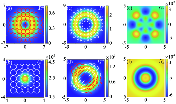
Figure S2: The polarization morphologies of incident VBs are shown for $j=1$ in (a) and $j=2$ in (c), and the tightly focused VBs on the focal plane for $j=1$ in (b) and $j=2$ in (d). The background color indicates the light intensity $I_{r}^{\rm{in}}=|\bm{\mathcal{E}}|^{2}$ and $I_{z}^{\rm{out}}=|E_{z}|^{2}$. White and red represent left-handed elliptical and right-handed elliptical polarization states, respectively. In (a) and (b), $m_{1}=2,l_{1}=-1,\alpha_{1}=\pi$; in (c) and (d), $m_{2}=1,l_{2}=3,\alpha_{2}=0.3\pi$. The spatial distributions of $\Omega_{r}$ and $\Omega_{z}$ are shown in (e) and (f), respectively. The spatial coordinates $x$ and $y$ are in units of trap size $a_{0}\equiv\sqrt{\hbar/M\omega}$.

In Fig. S2, we show the polarization and spatial distributions for specific VB parameters. In Fig. S2 (a), for $\alpha=0$ or $\pi$, the polarization distribution is homogeneous, and the VB corresponds to regular left- or right-circularly polarized light [19]. After passing through the tightly focusing system, the polarization reverses, as shown in Fig. S2 (b).

For $\alpha\neq 0$ or $\pi$, the beam exhibits a superposition of left- and right-circularly polarized components, resulting in a VB with a nonuniform polarization distribution, as shown in Fig. S2 (c). On the focal plane, this polarization distribution becomes more complex, as depicted in Fig. S2 (d). Additionally, the tight-focusing system also reduces spot size and increases intensity. Using these tightly focused VBs to couple atomic pseudospin levels, we obtain the spatial distributions of $\Omega_{r}$ and $\Omega_{z}$ shown in Fig. S2 (e) and (f).

S-5 spin texture

We analyze the spin textures in detail. Distinct from the SOAMC induced by LGBs [13, 14, 11, 15, 16, 17, 18, 9, 10], our scheme introduces a nonzero $\Omega_{z}$, resulting in a spatially dependent Zeeman shift term $\Omega_{z}\sigma_{z}$, providing an additional tunable degree of freedom. The spatial profile of $\Omega_{z}$ resembles a ring-shaped potential, as illustrated in Fig. S3 (g). The spin-up and spin-down components experience opposing external potentials, leading to a spin-polarized ground state. As $\alpha_{1}$ and $\alpha_{2}$ varies from 0 to $\pi$, the population peak locations shift, altering the density distribution of each spin component, with the positions of maximum population of spin-up or spin-down component labeled in Fig. S3 (g). For $\alpha_{1}=\alpha_{2}=0$ or $\pi$, the ground state becomes fully polarized with $\langle\sigma_{z}\rangle=\pm 1$, representing a topologically trivial structure. However, for intermediate values with $0<|\langle\sigma_{z}\rangle|<1$, the spin imbalance between the two spin states decreases. Specifically, for $\alpha_{1}=\alpha_{2}=0.37\pi$ and $0.45\pi$, we illustrate the density distributions and relative phases in Fig. S3 (a)-(f). The relative phases in Fig. S3 (c) and (f) show that the ground state exhibits a stable multiply quantized vortex with its quantized circulation to be $2\pi\times 5$.

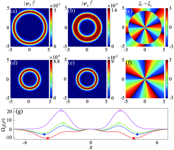
Figure S3: The ground state density profile $|\psi_{\sigma}|^{2}a_{0}^{2}/N$ and relative phase $\xi_{\uparrow}-\xi_{\downarrow}$ within the spatial range $x,y\in[-5a_{0},5a_{0}]$ for different ellipticity angles: (a)-(c) $\alpha_{1}=\alpha_{2}=0.37\pi$, (d)-(f) $\alpha_{1}=\alpha_{2}=0.45\pi$. (g) The spatial distribution of $\Omega_{z}$ along the $x$ axis at $y=0$. Red, blue, green, and magenta correspond to $\alpha_{1}=\alpha_{2}=0,0.37\pi,0.45\pi$, and $\pi$, respectively. Circle (square) labels the locations of maximum population of spin-up (spin-down) component. We set the other parameters $\beta_{1}=\beta_{2}=0$, $m_{1}=1$, $l_{1}=2$, $m_{2}=1$, $l_{2}=-4$, $\delta=0$, $\Omega_{0}=2.58\hbar\omega$, $\Omega_{s}=0$. The coordinates $x$ and $y$ are in units of trap size $a_{0}$.

The corresponding spin textures, as shown in Fig. 3 (c) and (d) of the main text, reveal topologically nontrivial giant skyrmion structures. To calculate the topological charge of skyrmion, we define a normalized complex-valued spinor $\mathbf{\chi}=[\chi_{\uparrow},\chi_{\downarrow}]^{T}=\left[|\chi_{\uparrow}|\mathrm{e}^{\mathrm{i}\xi_{\uparrow}},|\chi_{\downarrow}|\mathrm{e}^{\mathrm{i}\xi_{\downarrow}}\right]^{T}$, satisfying $|\chi_{\uparrow}|^{2}+|\chi_{\downarrow}|^{2}=1$. The wave functions can be expressed as $\psi_{\sigma}=\sqrt{\rho_{T}}\chi_{\sigma}$, with total density $\rho_{T}=|\psi_{\uparrow}|^{2}+|\psi_{\downarrow}|^{2}$. The pseudospin density is defined as $\mathbf{S}=\mathbf{\chi}^{\dagger}\vec{\sigma}_{\rm P}\mathbf{\chi}$ with $\vec{\sigma}_{\rm P}$ the Pauli matrix [20, 21, 22, 23]. The components of $\mathbf{S}$ are expressed as

$$S_{x}=2\left|\chi_{\uparrow}\right|\left|\chi_{\downarrow}\right|\cos(\xi_{\uparrow}-\xi_{\downarrow}),$$ (S33)

$$S_{y}=-2\left|\chi_{\uparrow}\right|\left|\chi_{\downarrow}\right|\sin(\xi_{\uparrow}-\xi_{\downarrow}),$$

$$S_{z}=|\chi_{\uparrow}|^{2}-|\chi_{\downarrow}|^{2},$$

and $|\mathbf{S}|^{2}=S_{x}^{2}+S_{y}^{2}+S_{z}^{2}=1$. In polar coordinates, the spin vector $\mathbf{S}$ can be written as

$$\mathbf{S}=(\sqrt{1-S_{z}^{2}}\cos(\Delta\kappa\varphi),\sqrt{1-S_{z}^{2}}\sin(\Delta\kappa\varphi),S_{z}),$$ (S34)

where the phases of two spin components can be approximately written as $\xi_{\sigma}=\kappa_{\sigma}\varphi$, with $\kappa_{\sigma}=0,1,2,...$ denoting the quantum number of the circulation of the spin component at radius $\rho$, and $\Delta\kappa=\kappa_{\uparrow}-\kappa_{\downarrow}$. For $\alpha_{1}=\alpha_{2}=0.37\pi$, $\kappa_{\uparrow}=5$, and $\kappa_{\downarrow}=0$ at the radii of both the inner and outer annular giant skyrmions. The corresponding topological charge density is written as $q(\bm{\rho})=\frac{\Delta\kappa}{4\pi\rho}\frac{dS_{z}(\rho)}{d\rho}$. Then we find the topological charges of giant skyrmions $Q_{\mathrm{in}}=\int\frac{\Delta\kappa}{4\pi\rho}\frac{dS_{z}(\rho)}{d\rho}\mathrm{d}\bm{\rho}=(\kappa_{\uparrow}-\kappa_{\downarrow})_{\mathrm{in}}=5$ and $Q_{\mathrm{out}}=-(\kappa_{\uparrow}-\kappa_{\downarrow})_{\mathrm{out}}=-5$. Increasing $\alpha_{1}$ and $\alpha_{2}$ to $\alpha_{1}=\alpha_{2}=0.45\pi$, we find a single giant skyrmion with topological charge $Q=-5$. Additionally, we perform calculations in the absence of $\Omega_{z}$, and find topologically trivial spin textures. This shows that the rich topological structures arise from the interplay of $\Omega_{z}$ and $\Omega_{r}$, demonstrating the high tunability of VB-induced gauge fields in exploring topological quantum phenomena.

References

• Richards and Wolf [1959] B. Richards and E. Wolf, Proceedings of the Royal Society of London. Series A. Mathematical and Physical Sciences 253, 358 (1959).
• Chen et al. [2012] Z. Chen, L. Hua, and J. Pu, Progress in Optics 57, 219 (2012).
• Yu et al. [2020] P. Yu, Y. Liu, Z. Wang, Y. Li, and L. Gong, Annalen Der Physik 532, 2000110 (2020).
• Le Kien et al. [2013] F. Le Kien, P. Schneeweiss, and A. Rauschenbeutel, Eur. Phys. J. D 67, 1 (2013).
• Goldman et al. [2014] N. Goldman, G. Juzeliūnas, P. Öhberg, and I. B. Spielman, Rep. Prog. Phys. 77, 126401 (2014).
• Zhai [2015] H. Zhai, Reports on Progress in Physics 78, 026001 (2015).
• Zhai [2021] H. Zhai, Ultracold atomic physics (Cambridge University Press, Cambridge, England, 2021).
• Chen et al. [2020a] K.-J. Chen, F. Wu, S.-G. Peng, W. Yi, and L. He, Physical Review Letters 125, 260407 (2020a).
• Zhang et al. [2019] D. Zhang, T. Gao, P. Zou, L. Kong, R. Li, X. Shen, X.-L. Chen, S.-G. Peng, M. Zhan, H. Pu, et al., Physical Review Letters 122, 110402 (2019).
• Chen et al. [2018] H.-R. Chen, K.-Y. Lin, P.-K. Chen, N.-C. Chiu, J.-B. Wang, C.-A. Chen, P. Huang, S.-K. Yip, Y. Kawaguchi, and Y.-J. Lin, Physical Review Letters 121, 113204 (2018).
• Qu et al. [2015] C. Qu, K. Sun, and C. Zhang, Physical Review A 91, 053630 (2015).
• Pethick and Smith [2018] C. J. Pethick and H. Smith, Bose-Einstein condensation in dilute gases (Cambridge University Press, Cambridge, England, 2018), 2nd ed.
• DeMarco and Pu [2015] M. DeMarco and H. Pu, Physical Review A 91, 033630 (2015).
• Sun et al. [2015] K. Sun, C. Qu, and C. Zhang, Physical Review A 91, 063627 (2015).
• Hu et al. [2015] Y.-X. Hu, C. Miniatura, and B. Gremaud, Physical Review A 92, 033615 (2015).
• Chen et al. [2016] L. Chen, H. Pu, and Y. Zhang, Physical Review A 93, 013629 (2016).
• Chen et al. [2020b] L. Chen, Y. Zhang, and H. Pu, Physical Review Letters 125, 195303 (2020b).
• Peng et al. [2022] S.-G. Peng, K. Jiang, X.-L. Chen, K.-J. Chen, P. Zou, and L. He, AAPPS Bulletin 32, 36 (2022).
• Rosales-Guzmán et al. [2018] C. Rosales-Guzmán, B. Ndagano, and A. Forbes, Journal of Optics 20, 123001 (2018).
• Wang et al. [2017] H. Wang, L. Wen, H. Yang, C. Shi, and J. Li, Journal of Physics B: Atomic, Molecular and Optical Physics 50, 155301 (2017).
• Jin et al. [2013] J. Jin, S. Zhang, W. Han, and Z. Wei, Journal of Physics B: Atomic, Molecular and Optical Physics 46, 075302 (2013).
• Yang et al. [2008] S.-J. Yang, Q.-S. Wu, S.-N. Zhang, and S. Feng, Physical Review A—Atomic, Molecular, and Optical Physics 77, 033621 (2008).
• Su et al. [2024] X. Su, W. Dai, T. Li, J. Wang, and L. Wen, Chaos, Solitons & Fractals 184, 114979 (2024).