Spin-imbalance induced buried topological edge currents in Mott & topological insulator heterostructures.
Abstract
We theoretically investigate the heterostructure between a ferrimagnetic Mott insulator and a time-reversal invariant topological band insulator on the two-dimensional Lieb lattice with periodic boundary conditions. Our Hartree-Fock and slave-rotor mean-field results incorporate long-range Coulomb interactions. We present charge and magnetic reconstructions at the two edges of the heterostructure and reveal how buried topological edge modes adapt to these heterostructure edge reconstructions. In particular, we demonstrate that the interface magnetic field induces a spin imbalance in the edge modes while preserving their topological character and metallic nature. We show that this imbalance leads to topologically protected buried spin and charge currents. The inherent spin-momentum locking ensures that left and right movers contribute to the current at the two buried interfaces in opposite directions. We show that the magnitude of the spin-imbalance induced charge and spin current can be tuned by adjusting the spin-orbit coupling of the bulk topological insulator relative to the correlation strength of the bulk Mott insulator. Thus, our results demonstrate a controlled conversion of a spin Hall effect into an analog of a charge Hall effect driven by band topology and interaction effects. These topologically protected charge and spin currents pave the way for advances in low-energy electronics and spintronic devices.
I Introduction
The need for sources of dissipationless current sources in electronic devices is ubiquitous. Stable spin current sources are essential for advancing spin-based electronics such as spin logic circuits to spin-based sensors and allow for increased energy efficiency Yang (2016). Spin current sources are essential in manipulating spin information within qubits, the critical ingredient of quantum computers Nayak et al. (2008). Similarly, charge currents that can flow without scattering are vital for low-energy electronics. However, the realization of dissipation-free current sources continues to face severe roadblocks. Perturbations such as spin relaxation, disorder and damping effects, temperature sensitivity, interface scattering, quantum tunneling and interference, and many-body effects are detrimental to reliable dissipationless spin and charge current sources at room temperature Hirohata et al. (2020). Protection against such generic agencies is difficult to guarantee, given the wide range of energy and length scales involved in these perturbations.
In this regard, topologically protected edge modes in time-reversal symmetric (TRS) band topological insulators (TI) that support helical edge modes with spin momentum locking are obvious candidates for dissipationless spin currents. However, magnetic impurities at the edge of a time-reversal-invariant (TRS) band-topological insulator (TI)Kane and Mele (2005a, b) can induce scattering between left and right movers due to the lifting of Kramer’s degeneracyHasan and Kane (2010). The edges are expected to lose their topological protection in such a situation. Moreover, the helical edges only support dissipationless spin-currrents in the ideal case. It is unclear if TRS-TI can be tweaked to support topologically protected charge currents. Can the magnetic field-induced TRS-breaking be turned from a foe to a friend Durnev and Tarasenko (2016); Ma et al. (2015)?
The interplay of strong correlation-induced magnetism and topology from spin-orbit has thus been actively investigated. The interplay of interaction effect on BTI edge modes has been studied on the Bernevig-Hughes-Zhang (BHZ) modelBernevig et al. (2006). Within Dynamical Mean Field Theory (DMFT)Amaricci et al. (2017, 2018) and considering interaction and spin-orbit coupling on the same region of the lattice in a strip geometry, the existence of topologically protected metallic edge mode has been established in the paramagnetic regime. The BHZ TI model kept in proximity to a paramagnetic Mott insulator (MI), has been shown to support metallic edge models along with interesting edge reconstructionsIshida and Liebsch (2014). Finally, paramagnetic DMFT solution on interacting square lattice with spin-orbit interactions sandwiched between two Mott insulators have described the nature of metallic state induced in the edge layers of the Mott insulatorsUeda et al. (2013).
However, the fate of the edge modes when the magnetic field is induced by proximity to a magnetic Mott insulator retaining the heterostructure geometry and contending with the complications from spin and charge reconstructions has received little attention. Such a situation can be engineered by considering a heterostructure of a strong-correlation-driven magnetic Mott insulator and a band topological insulator (BTI). This situation allows studying magnetic field effects on ‘buried’ helical edge modes.
From a general standpoint, heterostructures of dissimilar materials have yielded several surprises. The most striking example has been the demonstration of high mobility two-dimensional electron gasOhtomo and Hwang (2004) superconductivityGariglio et al. (2009) ferromagnetismBert et al. (2011) and magnetoresistenceBen Shalom et al. (2010) in the heterostructure of LaAlO3 and SrTiO3, a band and a Mott insulator respectively. This has spawned a huge body of investigation in correlated heterostructures Okamoto and Millis (2004a); Ueda et al. (2012); Borghi et al. (2010, 2010); Helmes et al. (2008); Euverte et al. (2012); PhysRevB.84.085103. In addition, junctions of superconductor-topological insulatorQi and Zhang (2011); Stanescu et al. (2010) and junctions between topological insulatorsRauch et al. (2013) are being actively being investigated.
In this spirit, we consider the heterostructure of a TRS-TI and a ferrimagnetic Mott insulator to examine the fate of buried topological edge modes. However, such an investigation has to tackle spin, charge, and magnetic reconstructions as is well-known in conventional MI and band insulator (BI) Chakhalian et al. (2014); Borghi et al. (2010). These reconstructions require modeling long-range Coulomb interaction along with local Hubbard-model-type interaction effectsOkamoto and Millis (2004b). Treating such interaction effects by interfacing with spin-orbit coupled TI can help answer several outstanding questions. These include how edge modes form when the TI edges hybridize with the magnetic MI (unlike TI with open boundary conditions). How do the edge modes accommodate the induced magnetization arising from the above-mentioned heterostructure edge reconstruction? What is the nature of spin and charge transport? Finally, what is the impact of different kinds of edge termination on buried edge modes? In this paper, we address these questions within the following setup.
For our study, we consider an underlying Lieb lattice in two dimensions. The heterostructure is constructed by stabilizing the Mott insulator with Hubbard repulsion on all sites on one half of the lattice and a topological insulator with spin-orbit coupling on the other. In addition, we consider long-range Coulomb interaction over the entire lattice. We employ unrestricted Hartree Fock mean field theory (HF) that allows direct access to magnetism to show that the ferrimagnetic order in the Mott insulator induces a spin imbalance among the edge modes. We compute spin-resolved edge currents to show that the proximity-induced spin imbalance induces a topologically protected spin-polarized current. We then demonstrate the tunability of the spin-polarized current with interaction and spin-orbit coupling. We support the mean-field conclusion of the existence of the edge modes for large interaction strengths using a strong interaction slave rotor (SR) mean-field approachFlorens and Georges (2004); Zhao and Paramekanti (2007) where we also incorporate long-range Coulomb interaction effects.
We report several significant findings. We demonstrate the charge and magnetic edge reconstruction at the heterostructure interface with different kinds of junction geometries. We establish that the magnetic field at the interface induces a spin imbalance in the edge modes while preserving the helical nature of the metallic edge modes. We show that the spin imbalance leads to the conversion of the pure spin current into a topologically protected charge current. We also demonstrate that the magnitude of these induced spin and charge currents can be tuned by controlling the spin-orbit coupling of the bulk topological insulator relative to the correlation strength of the bulk Mott insulator. Through this work, we thus demonstrate a controlled conversion of the spin Hall effect into an analog of the charge Hall effect, driven by band topology and interaction effects.
The paper is organized as follows: In Sec. II we present the heterostructure model, method and observables we compute. We discuss the results in Sec. III. We conclude the paper in Sec. IV.
II Model, method & Observables
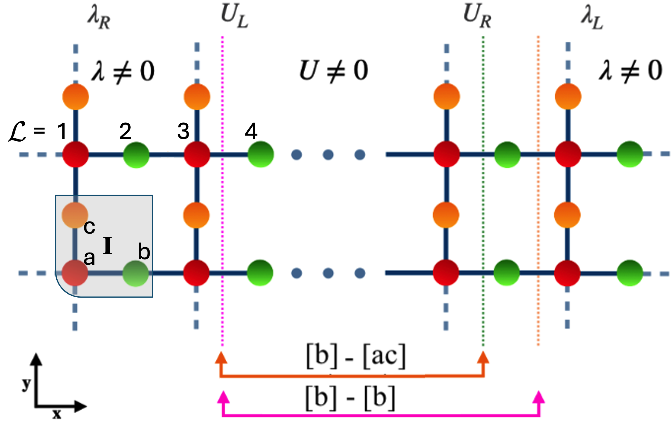
The Hamiltonian for the heterostructure defined on the Lieb lattice, Fig. 1, is as follows:
| (1) | ||||
Here, denotes the union of lattice points of whole heterostructure lattice with and are the set of the lattice sites of the and sides. and are electronic creation and annihilation operators respectively for spin state . refers to nearest neighbor hopping amplitude, while is the spin-orbit coupling involving next-nearest neighbors hopping. depending on the clockwise/anti-clockwise traversal of electrons around the ’a’ sites. This fact is encoded using and are the two unit vectors along the two nearest-neighbor bonds connecting ‘a’ sites to the ‘b’ and ‘c’ sites respectivelyWeeks and Franz (2010). Lastly, denotes the third Pauli matrix in spin space with components . We note that the spin-orbit coupling does not mix the spin species and should be considered a chirality-inducing term. The long-range Coulomb interaction between all the charges is taken into account via a self-consistent solution of the Coulomb potential. It is crucial to incorporate the long-range Coulomb interaction to control the amount of charge transferred across the interface. At a site , the Coulomb potential is defined as . The long-range Coulomb interaction Hamiltonian at a mean-field level as in literature Salafranca et al. (2008); Pradhan and Kampf (2013) is as follows:
| (2) |
where and is the Coulomb potential at site . In the definition of , are electron charge densities, runs over all lattice sites and , with and a denoting the dielectric constant and the lattice parameter, respectively. . The background charge is assumed to be for all sites. We assume a half-filled lattice with . We also employ two additional notations in the paper to analyze the results. Firstly, a unit-cell based label where is the unit cell index and refers to the atom of the unit cell and secondly a layer-label . These are shown in Fig. 1.
Hartree-Fock treatment: The interaction term in Eq. 1 is first treated within the HF mean field theory. The mean field self-consistency is carried out along the x-direction while translation invariance is assumed in the y-direction (as defined in Fig. 1). This allows us to define the eigenstates as a function of . To set up notation, we define the Hartree-Fock mean-field eigenvalues and eigenvectors as and respectively. We note that while translation invariance is imposed along the y direction, can vary with the unit cell index along x. We also construct ’layer-projected eigenvectors’ labeled by the index as indicated in Fig. 1.
The mean field solution of Hamiltonian Eq. 1 is discussed in Appendix A.1. The mean field solution is used in the calculation of the Coulomb potential as presented in Appendix A.2. Finally, in Appendix A.3, we provide details of the mean-field self-consistency and iterations.
From the HF calculations we compute the unit-cell resolved density of states (DOS) , where refers to unit-cell index along the x-direction, as discussed above. We also compute the spin resolved unit cell dependent band-dispersions, . To track unit cell dependence of magnetization, we compute the magnetization of the unit-cell averaged over sites in the unit cell.
In Appendix A.4, we derive the expression of the charge current at a unit cell of the heterostructure. A brief discussion is given below.
| (3) | ||||
where and . Now defining spin resolved current flowing in positive direction along ‘x’ as and along positive ‘y’ as , we can express the total charge current flowing in direction is . Similarly, defines the spin current along y.
Slave-rotor treatment: We use the standard SR strong-interaction mean-field approach to corroborate the Hartree-Fock results. While the SR approach cannot capture magnetic order, it allows calculation of the Mott gap and Mott to metal transition retaining charge fluctuations, which is missed in Hartree-Fock theory. In the present work, we carry out the SR approach in a non-uniform charge density background due to the Coulomb potential. The details of this calculation are given in Appendix B.1.
The main observable in our SR calculation is the unit-cell resolved density of states defined and extracted from the SR single-particle Green’s function, as derived in Appendix B.2.
III Results
We present results for two kinds of heterostructure [b]-[ac] and [b]-[b] as shown in Fig. 1. We first discuss the unrestricted Hartree-Fock (HF) mean field results and then discuss the (SR) results.
III.1 Unit cell-resolved DOS & buried topological edge modes
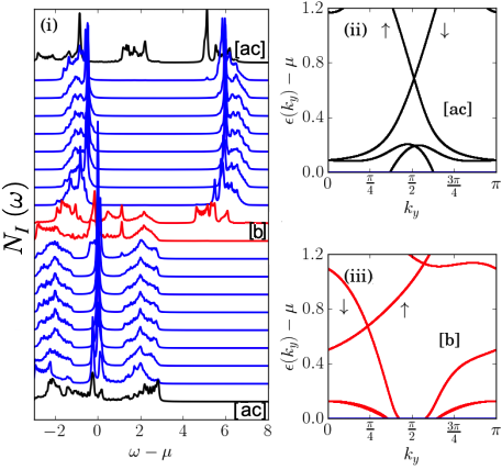
Fig. 2 (i) shows the unit-cell resolved density of states (DOS) for [b]-[ac] heterostructure from the HF calculations. The unit-cell-resolved DOS is plotted from the bottom (the terminating unit cell of the region at the or [ac] interface) to the middle with two red unit cells one on either side of the or [b] interface, and going up to the top (the remaining terminating unit cell of the region at the or [ac] interface). The DOS of the interface unit cells colored in red and black are of particular interest to us. The DOS of the remaining unit cells are shown in blue. In the plot, demarcates the global chemical potential. For the bulk unit cells, the DOS shows a bulk gap and the lower and upper Hubbard sub-bands as expected Costa et al. (2016); Oliveira-Lima et al. (2020). For the bulk, we recover the Lieb lattice spectrum supporting two dispersive bands and a flat band, with a separation of from both the dispersive bandsWeeks and Franz (2010). The DOS of the red and black unit cells both show finite spectral weight spread over in the energy regime where the respective bulk DOS have gaps. The spin-resolved band dispersion along arising out of the unit cells corresponding to the red ([b] edge) and black ([ac] edge) DOS of Fig. 2 (i) are shown in Fig. 2 (ii) and Fig. 2 (iii). Comparison with Fig. 2 (i) shows that the edge modes are constructed from the spectral weight in the energy windows of the bulk gap seen for the red and black unit cells. We find clear spin-momentum locking, as is expected, at the edge of a topological band insulator. For clarity, we have only shown the edge mode above the Fermi energy; the same spin-momentum locking is seen for the edge modes below the Fermi energy.
At the edge of a conventional time-reversal symmetric band topological band insulator, the currents for the up and the down spin carriers are equal in magnitude, and the system supports helical spin currents. However, as a main result of the paper, we demonstrate that these buried edge modes are quite different from those in the conventional case. Due to the ferrimagnetic state of the Mott insulator, a spin imbalance is induced on the edge unit cells, leading to a finite charge current instead of a pure spin current. To elucidate the physics, we first discuss the reconstruction of the charge and magnetism across the heterojunction.
III.2 Edge reconstruction
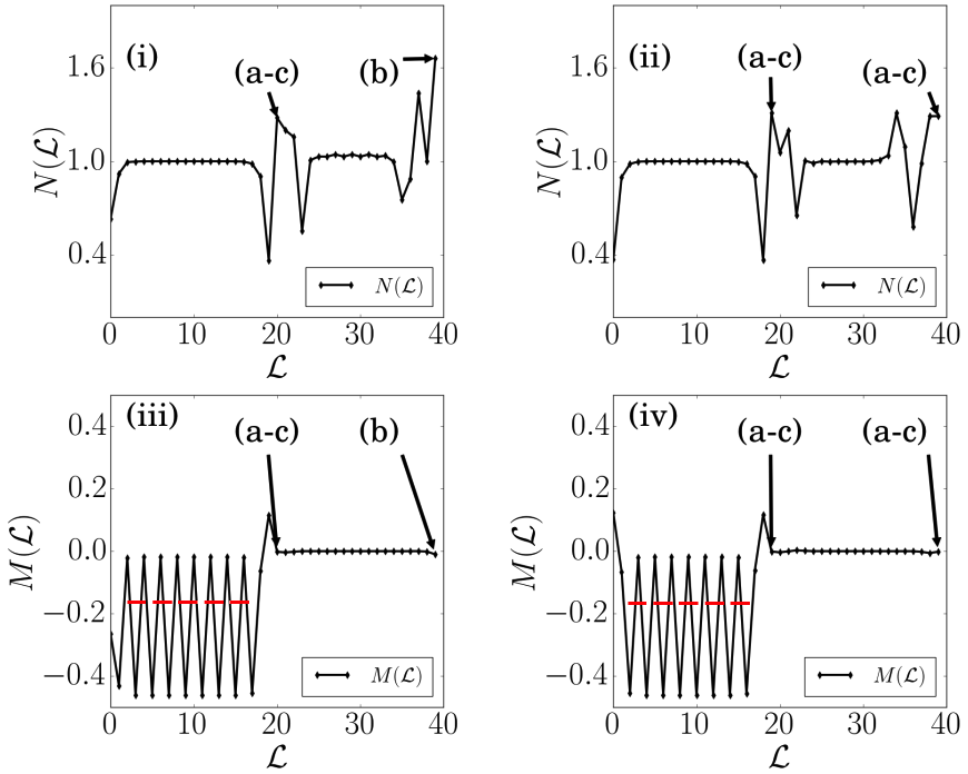
We first discuss the charge reconstruction as we traverse across the interfaces, shown in Fig. 3 (i) for the [b]-[ac] heterostructure. Fig.3 (i) and (iii) show the layer () resolved charge density profile (black curve) and magnetization for a fixed and respectively. In Fig. 3 (i) along the x-axis, alternate layers are composed of (a-c) and (b) sites as can be seen from Fig. 1. The (a-c) and (b) sites of the region interfacing with the region are marked by arrows in Fig. 3 (i). The density and the magnetization are averaged over all (a-c) sites and (b) sites in each layer.
From Fig. 3 (i), we find that the average density per site in the bulk and bulk is 1. The half-filling triggers a Mott insulating state in the bulk layer. The Mott state in the bulk region is characterized by the Mott-lobes separated by as seen in the DOS in Fig. 2 (i). Similarly, the bulk behaves as a half-filled Lieb lattice. We note substantial charge-density reconstruction at the interface that causes the filling to deviate locally from . As a result, the edge states are partially filled. For the (a-c) and (b) layers of the side interfacing with the side, the average charge densities are larger than 1 that is compensated by strong suppression of change density of the interfacing layers of the side. The charge reconstruction induces a self-doping of the interface layers contributing to the buried metallic edge modes between a Mott and a TRS topological insulator.
From Fig. 3 (iii), we find an alternating magnetization profile in the Mott regime with a non-zero average value (dashed horizontal line) as expected from the Lieb’s theoremLieb (1989), thus stabilizing a ferrimagnetic Mott insulator. We note that for the layers with (a-c) sites, the magnetization is depicted as an average value, while for the layers with (b)-sites, the magnetization is provided for the (b) site only. The net non-zero magnetization is computed by average unit cell magnetization (), defined earlier. The same convention is followed for the side. The bulk-magnetization of the side is zero. However, for the unit cells on the left [b] and right [ac] interfaces, the average unit cell magnetization for the side are -0.0026 and -0.0043, respectively. In the following subsection, we discuss the importance of this small negative magnetization on the edge currents.
In Fig.3 (ii) and (iv), we show the results for the [b]-[b] heterostructure. While the broad phenomenology remains the same, we see the change in the charge and magnetization reconstruction when the [b] edge is replaced by [ac] edge at layers and 39.
III.3 Charge & spin currents:
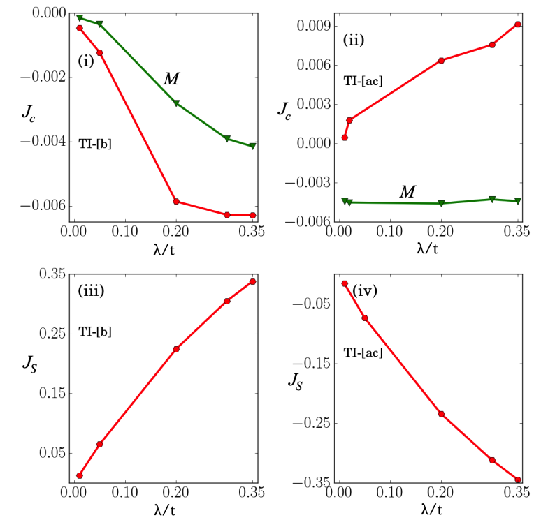
We show the edge currents and magnetization for the [b]-[ac] heterostructure in Fig. 4 for various values for the two edges on the topological side. Numerically, for the calculation parameters, the charge current (), the spin current (), and the magnetization () penetrate up to three unit cells at the interface on the TI side (along the x direction). Hence, the results are shown by averaging , and over these three unit-cells. Similarly, averaged quantities are shown for the [ac] edge.
Fig. 4 panels (i) and (ii) respectively show the charge current () and for the [b] and [ac] edges on the topological side. For all the values, the induced magnetization at the TI edge is negative. The negative magnetization induces an increased down-spin occupation of the edge states at both [b] and [ac] edges. However, from Fig. 2 (iii) and (ii), we find that the spin-momentum locking implies that the down spin electrons contribute to current along the negative y-direction for the [b] edge. In contrast, it contributes to current along positive y-direction at the [ac] edge. We emphasize that the edge modes in Fig. 2 (iii) and (ii) are also computed, including contributions from three edge unit cells. For zero magnetization of the edge (for example, a TRS TI on the Lieb lattice interfacing with vacuum, the edge currents in opposite directions would be equal in magnitude. That would imply a net zero , but a finite spin current equal to . The charge current is clearly finite in the presence of the induced negative magnetization. It flows in the negative y-direction for the [b] edge and the positive y-direction for the [ac] edge. In addition, the edges support finite . Fig. 4 (iii) and (iv) show the spin current () as a function of for for the [b] and the[ac] edge,s respectively. As expected, the spin current magnitudes for both edges increase with . However, unlike for a TRS-TI interfacing with vacuum, a part of the spin current is converted to the charge current due to the induced magnetic field at the edge. We emphasize that the full heterostructure is characterized by a common spin quantization axis, and only a weak magnetization is induced at the edge modes. Thus, the spin-momentum-locked helical nature of the edge states and the ensuing topological protection survive even in the presence of TRS breaking at the edge. Hence, we have shown a mechanism of converting a spin current into a charge current, which is equivalent to converting a spin-Hall effect to a charge Hall effect analog driven by band topology.
III.4 Slave-rotor results
The advantage is that SR mean field theory retains charge fluctuations that are not captured in HF theory. However being a paramagnetic approach, it can only capture Mott-metal transition and misses out on magnetic order, as is true for the paramagnetic DMFT calculations. Thus, the SR is used here to demonstrate the validity of the HF result of the existence of the edge modes despite the large interfacing with the TI. The SR calculations, as discussed in Appendix B, are performed on the background of the Coulomb potential.
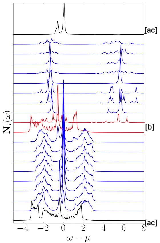
Fig. 5 shows the layer resolved DOS from SR mean-field theory for the [b]-[ac] heterostructure. The results presented are analogous to the HF results in Fig. 2 (a). The bulk of the region supports a many-body Mott gap. Note that the sharp nature of the upper and lower Hubbard sub-bands arises from a cluster treatment of the rotor Hamiltonian, as discussed in Appendix B. The bulk region shows TRS-TI band structure on the Lieb lattice. Finally, the interface layers for both the [b] and the [ac] edges show spectral weights that interpolate the bulk bands, indicating the same phenomena as in the HF theory. The appearance of the sharp peak at the Fermi energy in the interface unit-cells of the Mott regime is the well-known mid-gap resonanceKajueter et al. (1996) of doped Mott insulators. They arise out of Kondo screening of gapless spin states of Mott insulators by the carriers of the helical edges that penetrate the first unit cell of the MI at these two interfaces. Such mid-gap states have also been observed in MI/TBI heterostructureUeda et al. (2013). Note that such many-body effects in SR mean-field theory cannot be captured in the HF calculations. Thus, the SR results show the robustness of the helical edge modes even when many-body charge fluctuation effects are included.
The interplay of strong correlation-induced magnetism and topology from spin-orbit has thus been actively investigated. The interplay of interaction effect on BTI edge modes has been studied on the Bernevig-Hughes-Zhang (BHZ) modelBernevig et al. (2006). Within Dynamical Mean Field Theory (DMFT)Amaricci et al. (2017, 2018) and considering interaction and spin-orbit coupling on the same region of the lattice in a strip geometry, the existence of topologically protected metallic edge mode has been established in the paramagnetic regime. The BHZ TI model kept in proximity to a paramagnetic Mott insulator (MI), has been shown to support metallic edge models along with interesting edge reconstructionsIshida and Liebsch (2014). Finally, paramagnetic DMFT solution on interacting square lattice with spin-orbit interactions sandwiched between two Mott insulators have described the nature of metallic state induced in the edge layers of the Mott insulatorsUeda et al. (2013).
IV Conclusion
In previous works on MI/TI interfaces, electron interaction, and spin-orbit effects were simultaneously present in the TI region Amaricci et al. (2017, 2018) . Further, while inhomogeneous DMFT was employed in earlier work, long-range Coulomb interaction effects were not considered, and only paramagnetic DMFT solutions were evaluated. Thus, buried interfaces of genuine TRS band TI and MI could not be studied as the Coulomb potential is crucial in avoiding electronic phase separation. Even in the cases examined, the paramagnetic calculationsIshida and Liebsch (2014); Ueda et al. (2013) have prevented any insight into the magnetic nature of the topological edge mode. Thus, the effect of induced magnetism on TRS-TI buried edges has remained open.
We have studied the interplay between interaction effects and spin-orbit coupling at the MI-TI interface in Lieb lattice heterostructure geometry. The MI has a ferrimagnetic order, while the TI hosts a bulk topological phase. Upon hybridization, solving the Hartree-Fock problem, and self-consistent evaluation of the Coulomb potential, we find that the metallic edge modes survive despite the edges being subject to finite magnetization. The full heterostructure has a common spin quantization axis, and the induced magnetization in the helical edge modes is small. Due to this, the topological protection survives. In addition, the Hartree-Fock results show that the induced magnetization at the TI interface unit cells causes a spin imbalance in the edge modes. We demonstrate that this imbalance stabilizes a charge current at the interface that is topologically protected. The current can be controlled by tuning the spin-orbit coupling strength and the interface geometry. We also support the validity of edge modes from Hartree-Fock by using strong coupling paramagnetic slave-rotor theory that captures charge fluctuation.
The Lieb lattice is easily realized in layered transition metal oxides with perovskites structure Fina et al. (2014); Sardar et al. (2024). We envision a 3d/5d layered perovskite heterostructure as a natural candidate to realize such topologically protected partially spin-polarized charge currents. The tuning of the parameters can be achieved by choosing differing combinations of the 3d (with strong correlations) and 5d (strong spin-orbit coupling) transition metal atoms. Such controlled current sources can be used in electronics and spintronic devices to reduce heat generation.
Acknowledgements.
We acknowledge the usage of VIRGO and NOETHER computational clusters at NISER. A.M. would also like to acknowledge SERB-MATRICS grant (Grant No. MTR/2022/000636) from the Science and Engineering Research Board (SERB) for funding. K.S. would also like to acknowledge SERB-MATRICS grant (Grant No. MTR/2023/000743) from the Science and Engineering Research Board (SERB) for funding.Appendix A Hartree-Fock approach
A.1 Mean field in k-space
This section outlines the HF mean-field formalism introduced in section II. The interacting Hubbard Hamiltonian is given by
| (A1) |
We employ the mean-field approximation to simplify the two-body interaction term. This involves decoupling the product of number operators as
| (A2) |
Under this approximation, the interaction Hamiltonian takes the following form:
| (A3) |
where is the total on-site occupation and is the on-site magnetization. The second term in Eq. A3 introduces a global constant energy shift and can, therefore, be neglected as it does not affect the relative energy spectrum of the system. The resulting interacting Hamiltonian in momentum space is
| (A4) |
where is conjugate momenta along the translation invariant direction and denotes sites within the unit cell as shown in Fig.1. and respectively. Here and are calculated self consistently.
A.2 Long-range Coulomb interaction
The average electron density of the MI and TI in the heterostructure is determined by the chemical potential . The long-range Coulomb interaction between all charges is crucial in controlling the amount of charge transfer across the interfaces. To account for this effect, we solve the Coulomb potentials self-consistently at the mean-field level, following the methodology established in the literature Salafranca et al. (2008); Pradhan and Kampf (2013). The Hamiltonian describes the long-range Coulomb interaction:
| (A5) |
where,
In this equation, represents the electron charge density at the site () and is the Madelung constant, as defined in the paper. Throughout the calculations, we assume a uniform background charge . Solving self-consistently allows us to incorporate the long-range Coulomb interaction effect on the charge transfer across the MI-TI interface, ensuring that the electrostatic effects are treated consistently within the mean-field framework.
A.3 Computational details of self-consistency in Hartree-Fock approach
We performed self-consistent calculations of the mean-field parameters and . We set the convergence tolerance in energy to be . Additionally, we fixed the Madelung constant to throughout all calculations to ensure a uniform electron density within the bulk on each side of the heterostructure. We have averaged the Coulomb potential within the side, leaving two unit cells from each end of the side.
A.4 Derivation of current
In section II of the main text, we briefly outlined the prescription to calculate the current operators. In this section, we provide derivation of current operators. We start be rewriting the Hamiltonian in a slightly convenient notation. This Hamiltonian Eq. 1 can be separated into three components:
| (A6) |
where is the hopping Hamiltonian, describes the spin-orbit coupling
and represents the onsite Hubbard interaction .
In the mean-field approximation , simplifying the analysis. The hopping and spin-orbit coupling terms are rewritten in terms of the unit cell index . The hopping Hamiltonian becomes
| (A7) |
The spin-orbit coupling Hamiltonian is expressed as
| (A8) |
The local Hubbard interaction term is expressed as:
| (A9) |
where is the strength of the on-site Hubbard interaction , for . and are the next-nearest lattice translation vector relative to the unit cell in the positive and direction respectively. Using these Hamiltonians, the current operators are derived by summing over contributions from all unit cells in a specific direction. The current operator in the -direction is found to be
| (A10) | ||||
Similarly, the current operator in the -direction is
| (A11) | ||||
These expressions are derived under the assumption that adjacent layers exist on both sides of the layer that is being considered for the current calculation, i.e., for bulk layers.
Appendix B Slave-rotor mean field theory
We study the correlation effects in the heterostructure using the slave-rotor mean-field theory, as outlined in previous works Florens and Georges (2004); Zhao and Paramekanti (2007); Jana et al. (2019). To make this study self-contained, we briefly summarize the method here. The electronic creation and annihilation operators are decomposed into a direct product of a bosonic rotor degree of freedom and an auxiliary fermion. The rotor accounts for charge occupations, while the spinons preserve the antisymmetric nature of the electronic operators. To distinguish between the two sides of the heterostructure, we denote the electronic operator on the -side as and on the -side as . Specifically, the transformations are:
| (B1) |
We then apply the slave-rotor decomposition to the -side as follows:
| (B2) |
where , are spinon creation and annihilation operators and represent the rotor creation and annihilation operators. The rotor operators act on charge states as
| (B3) |
To ensure that the spin and the charge degrees of freedom add up to physical electron occupation in the unit cell, we need to restrict the rotor spectrum. At half-filling, the average occupation of every unit cell is three. To remove the unphysical states from the direct product basis, we impose the following constraint equation
| (B4) |
where the electron number is equal to the spinon number i.e. and is the identity operator.
Then, the Hamiltonian Eq. 1 is reformulated in terms of spinon and rotor operators to derive an exact expression under the slave-rotor decomposition. Subsequently, we introduce a mean-field ansatz to approximate the ground state:
| (B5) |
where the superscript denotes the collective index for the electronic operators on the -side, refers to the spinon operator on the -side, and denotes the rotor operator. The Hubbard interaction term is confined exclusively to the -side, resulting in the spinon contribution emerging solely from the -side. The next step is to compute two decoupled Hamiltonians, and . The expressions are:
| (B6) | ||||
| (B7) | ||||
where are onsite Coulomb potentials as discussed in Eq.(2). The two coupled Hamiltonians are solved self-consistently under the constraint equation. The spinon Hamiltonian refers to Eq.B6 a one-body physics, while the rotor Hamiltonian in Eq.B7 describes many-body physics which can be solved using cluster mean-field theory. Since the system is inhomogeneous, we solve using multiple unit cell clusters along the -direction and repeat this in the -direction.
B.1 Observable in Slave-rotor calculation
We express the single-particle electron Green’s function as a convolution of the spinon and rotor Green’s functionsPaul et al. (2019). By taking the imaginary part of this reconstructed Green’s function, we compute the spectral function. We define the local (on-site) retarded Matsubara Green’s function as
| (B8) |
The spinon correlation function in Eq. (B8) is
| (B9) |
where and are the spinon eigenvectors and eigenvalues, respectively. The rotor correlation function in Eq. (B8) is expressed as
| (B10) |
where and are the eigenvalues and corresponding eigenvectors of the rotor Hamiltonian, respectively. Here, is the rotor partition function
| (B11) |
The integration in Eq. (B8) performed over imaginary time . We then analytically continue back to the real frequency to obtain . The projected density of state (PDOS ) is obtained from its imaginary part of the full Green function.
References
- Yang (2016) S. A. Yang, SPIN 06, 1640003 (2016), https://doi.org/10.1142/S2010324716400038 .
- Nayak et al. (2008) C. Nayak, S. H. Simon, A. Stern, M. Freedman, and S. Das Sarma, Rev. Mod. Phys. 80, 1083 (2008).
- Hirohata et al. (2020) A. Hirohata, K. Yamada, Y. Nakatani, I.-L. Prejbeanu, B. Diény, P. Pirro, and B. Hillebrands, Journal of Magnetism and Magnetic Materials 509, 166711 (2020).
- Kane and Mele (2005a) C. L. Kane and E. J. Mele, Phys. Rev. Lett. 95, 146802 (2005a).
- Kane and Mele (2005b) C. L. Kane and E. J. Mele, Phys. Rev. Lett. 95, 226801 (2005b).
- Hasan and Kane (2010) M. Z. Hasan and C. L. Kane, Rev. Mod. Phys. 82, 3045 (2010).
- Durnev and Tarasenko (2016) M. V. Durnev and S. A. Tarasenko, Phys. Rev. B 93, 075434 (2016).
- Ma et al. (2015) E. Y. Ma, M. R. Calvo, J. Wang, B. Lian, M. Mühlbauer, C. Brüne, Y.-T. Cui, K. Lai, W. Kundhikanjana, Y. Yang, M. Baenninger, M. König, C. Ames, H. Buhmann, P. Leubner, L. W. Molenkamp, S.-C. Zhang, D. Goldhaber-Gordon, M. A. Kelly, and Z.-X. Shen, Nature Communications 6, 7252 (2015).
- Bernevig et al. (2006) B. A. Bernevig, T. L. Hughes, and S.-C. Zhang, Science 314, 1757 (2006), https://www.science.org/doi/pdf/10.1126/science.1133734 .
- Amaricci et al. (2017) A. Amaricci, L. Privitera, F. Petocchi, M. Capone, G. Sangiovanni, and B. Trauzettel, Phys. Rev. B 95, 205120 (2017).
- Amaricci et al. (2018) A. Amaricci, A. Valli, G. Sangiovanni, B. Trauzettel, and M. Capone, Phys. Rev. B 98, 045133 (2018).
- Ishida and Liebsch (2014) H. Ishida and A. Liebsch, Phys. Rev. B 90, 205134 (2014).
- Ueda et al. (2013) S. Ueda, N. Kawakami, and M. Sigrist, Phys. Rev. B 87, 161108 (2013).
- Ohtomo and Hwang (2004) A. Ohtomo and H. Y. Hwang, Nature 427, 423 (2004).
- Gariglio et al. (2009) S. Gariglio, N. Reyren, A. D. Caviglia, and J.-M. Triscone, Journal of Physics: Condensed Matter 21, 164213 (2009).
- Bert et al. (2011) J. A. Bert, B. Kalisky, C. Bell, M. Kim, Y. Hikita, H. Y. Hwang, and K. A. Moler, Nature Physics 7, 767 (2011).
- Ben Shalom et al. (2010) M. Ben Shalom, M. Sachs, D. Rakhmilevitch, A. Palevski, and Y. Dagan, Phys. Rev. Lett. 104, 126802 (2010).
- Okamoto and Millis (2004a) S. Okamoto and A. J. Millis, Phys. Rev. B 70, 241104 (2004a).
- Ueda et al. (2012) S. Ueda, N. Kawakami, and M. Sigrist, Phys. Rev. B 85, 235112 (2012).
- Borghi et al. (2010) G. Borghi, M. Fabrizio, and E. Tosatti, Phys. Rev. B 81, 115134 (2010).
- Helmes et al. (2008) R. W. Helmes, T. A. Costi, and A. Rosch, Phys. Rev. Lett. 101, 066802 (2008).
- Euverte et al. (2012) A. Euverte, F. Hébert, S. Chiesa, R. T. Scalettar, and G. G. Batrouni, Phys. Rev. Lett. 108, 246401 (2012).
- Qi and Zhang (2011) X.-L. Qi and S.-C. Zhang, Rev. Mod. Phys. 83, 1057 (2011).
- Stanescu et al. (2010) T. D. Stanescu, J. D. Sau, R. M. Lutchyn, and S. Das Sarma, Phys. Rev. B 81, 241310 (2010).
- Rauch et al. (2013) T. c. v. Rauch, M. Flieger, J. Henk, and I. Mertig, Phys. Rev. B 88, 245120 (2013).
- Chakhalian et al. (2014) J. Chakhalian, J. W. Freeland, A. J. Millis, C. Panagopoulos, and J. M. Rondinelli, Rev. Mod. Phys. 86, 1189 (2014).
- Okamoto and Millis (2004b) S. Okamoto and A. J. Millis, Nature 428, 630 (2004b).
- Florens and Georges (2004) S. Florens and A. Georges, Phys. Rev. B 70, 035114 (2004).
- Zhao and Paramekanti (2007) E. Zhao and A. Paramekanti, Phys. Rev. B 76, 195101 (2007).
- Weeks and Franz (2010) C. Weeks and M. Franz, Phys. Rev. B 82, 085310 (2010).
- Salafranca et al. (2008) J. Salafranca, M. J. Calderón, and L. Brey, Phys. Rev. B 77, 014441 (2008).
- Pradhan and Kampf (2013) K. Pradhan and A. P. Kampf, Phys. Rev. B 88, 115136 (2013).
- Costa et al. (2016) N. C. Costa, T. Mendes-Santos, T. Paiva, R. R. d. Santos, and R. T. Scalettar, Phys. Rev. B 94, 155107 (2016).
- Oliveira-Lima et al. (2020) L. Oliveira-Lima, N. C. Costa, J. P. de Lima, R. T. Scalettar, and R. R. d. Santos, Phys. Rev. B 101, 165109 (2020).
- Lieb (1989) E. H. Lieb, Phys. Rev. Lett. 62, 1927 (1989).
- Kajueter et al. (1996) H. Kajueter, G. Kotliar, and G. Moeller, Phys. Rev. B 53, 16214 (1996).
- Fina et al. (2014) I. Fina, X. Marti, D. Yi, J. Liu, J. H. Chu, C. Rayan-Serrao, S. Suresha, A. B. Shick, J. Železný, T. Jungwirth, J. Fontcuberta, and R. Ramesh, Nature Communications 5, 4671 (2014).
- Sardar et al. (2024) S. Sardar, M. Vagadia, T. M. Tank, J. Sahoo, and D. S. Rana, Journal of Applied Physics 135, 080701 (2024), https://pubs.aip.org/aip/jap/article-pdf/doi/10.1063/5.0181284/19802168/080701_1_5.0181284.pdf .
- Jana et al. (2019) S. Jana, A. Saha, and A. Mukherjee, Phys. Rev. B 100, 045420 (2019).
- Paul et al. (2019) A. Paul, A. Mukherjee, I. Dasgupta, A. Paramekanti, and T. Saha-Dasgupta, Phys. Rev. Lett. 122, 016404 (2019).