Amortized Safe Active Learning for Real-Time Decision-Making: Pretrained Neural Policies from Simulated Nonparametric Functions

Abstract

Active Learning (AL) is a sequential learning approach aiming at selecting the most informative data for model training. In many systems, safety constraints appear during data evaluation, requiring the development of safe AL methods. Key challenges of AL are the repeated model training and acquisition optimization required for data selection, which become particularly restrictive under safety constraints. This repeated effort often creates a bottleneck, especially in physical systems requiring real-time decision-making. In this paper, we propose a novel amortized safe AL framework. By leveraging a pretrained neural network policy, our method eliminates the need for repeated model training and acquisition optimization, achieving substantial speed improvements while maintaining competitive learning outcomes and safety awareness. The policy is trained entirely on synthetic data utilizing a novel safe AL objective. The resulting policy is highly versatile and adapts to a wide range of systems, as we demonstrate in our experiments. Furthermore, our framework is modular and we empirically show that we also achieve superior performance for unconstrained time-sensitive AL tasks if we omit the safety requirement.

1 Introduction

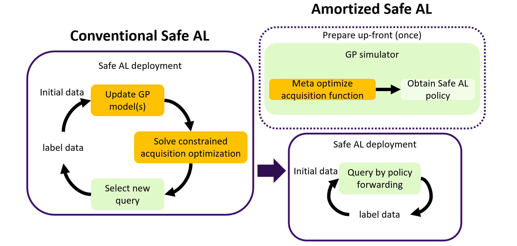
Figure 1: The conventional safe AL relies on computationally expensive (orange) GP fitting and constrained acquisition optimization. Our amortized AL approach meta trains a safe active learner up-front from synthetic data, allowing a fast, easy and real-time applicable (green) deployment.

Active learning (AL) is a sequential design of experiments, aiming to learn a task with reduced data labeling effort (Settles, 2010; Kumar & Gupta, 2020; Tharwat & Schenck, 2023). Each label is queried by optimizing an acquisition function, a function leveraging the current knowledge (typically model-based) to estimate the expected information gained from accessing new labels. AL is often discussed together with Bayesian optimization (BO), which aims to search global optima with limited evaluations (Srinivas et al., 2012; Brochu et al., 2010). The major difference is the acquisition function, where BO focuses only on candidate optima, while AL explores the complete space.

In many engineering (Zimmer et al., 2018; Berkenkamp et al., 2016) or chemical design problems (Griffiths & Hernández-Lobato, 2020), data evaluations can trigger safety concerns. The safety constraints cannot be directly mapped to the input space, motivating the development of safe AL (Schreiter et al., 2015; Zimmer et al., 2018; Li et al., 2022) and safe BO (Sui et al., 2015; Yanan Sui et al., 2018; Berkenkamp et al., 2020). These approaches introduce additional model(s) to quantify the safety conditions and leverage the safety knowledge to constrain the acquisition optimization (Figure 1 left). In these problems, Gaussian processes (GPs, Rasmussen & Williams, 2006) are a popular tool. A GP is a distribution over functions, which provides well-calibrated predictive uncertainty estimates that are well suited for modeling safety confidence (Sui et al., 2015; Schreiter et al., 2015; Zimmer et al., 2018).

Safe learning methods are prominent, capable of learning functions adaptively and safely, without requiring a parametric structure of the functions. However, the computation is heavy: (i) GPs scale cubically with the number of data points in time and are updated repeatedly; (ii) each data selection step solves an acquisition optimization, which can already be difficult for unconstrained learning (Swersky et al., 2020) and is even more complex under safety constraints (Sui et al., 2015; Schreiter et al., 2015). In particular, many physical systems require real-time decision-making (Nguyen–Tuong & Peters, 2010; Andersson et al., 2017; Lederer et al., 2021), which poses a significant challenge to employ these approaches. Various approximations have been investigated to make GP modeling more efficient (Titsias, 2009; Hensman et al., 2015; Bitzer et al., 2023), some of which have been adapted on scenarios of incremental data (Moss et al., 2023; Pescador-Barrios et al., 2024). However, and to the best of our knowledge, simplifying the repeated constrained acquisition optimization remains an open challenge.

In this paper, we focus on safe AL applications (Schreiter et al., 2015; Zimmer et al., 2018; Li et al., 2022), and we wish to amortize the effort of the data querying process. Prior to the deployment, we propose to learn an AL policy based on synthetic nonparametric functions. The policy is a neural network (NN) which suggests each new query with a simple forward pass (Figure 1 right) hereby replacing both the GP modeling and the constrained optimization. Our approach also benefits unconstrained AL of GPs, by omitting the safety constraints. Note that we use the term model to refer to the model one wishes to actively learn on a specific task, while the NN policy guides the data collections and the data are then fed to model the task.

In a nutshell, our approach (i) takes GPs as distributions of general nonparametric functions, (ii) utilizes a scalable random feature technique (Rahimi & Recht, 2007; Wilson et al., 2020) to generate functions in large scale, (iii) solves and meta learns AL decisions on those functions, and then (iv) zero-shot generalizes to real-world problems.

Contributions:

Our contributions are:

• We propose an NN policy for safe AL and, as an intermediate contribution, for unconstrained AL, that suggests new queries based on previously recorded data, hereby completely replacing the costly GP modeling and acquisition optimization steps during deployment;

• We demonstrate that our policy leads to a tremendous speed gain, allowing for real-time applications, while still (i) showing competitive data quality for both unconstrained and safe AL, i.e. collected data lead to competitive modeling performance, and (ii) being safety aware when required;

• Our policy is trained up-front exclusively on synthetic data, which represents a broad class of nonparametric functions, and generalizes to a multitude of systems;

• In order to train our safe AL policy, we propose a differentiable safety-aware acquisition criterion in closed form, which serves as an objective function in our pretraining environment.

Related works:

Safe learning often employs GPs. Gelbart et al. (2014) proposed a constrained BO, discounting the acquisition scores by a GP safety confidence, assuming the acquisition function is non-negative. Schreiter et al. (2015); Sui et al. (2015) proposed to constrain the acquisition optimization by the GP safety confidence, leading to a learning scheme with probabilistic safety guarantees. This scheme was then extended to systems with multiple safety constraints (Berkenkamp et al., 2020), to time-series modeling (Zimmer et al., 2018), and to safe multi-task learning (Li et al., 2022) as well as transfer learning (Li et al., 2024). Another scheme of constrained sequential decision-making is safe reinforcement learning (García et al., 2015; Brunke et al., 2022; Gu et al., 2024). This is often based on a constrained Markov decision process, where an agent learns to make safe actions on states (given Markov property) (Altman, 1999). These safe learning methods employ significant computations, impeding their deployment in real-time decision-making problems.

Recently, various meta learning approaches have been investigated to streamline sequential learning methods. Rothfuss et al. (2021) proposed to meta learn GP hyperparameters from existing tasks, simplifying GP modeling in safe BO. Liu et al. (2020b); Bitzer et al. (2023) proposed to pretrain from synthetic data to infer the GP model parameters. On the acquisition phase, Swersky et al. (2020) proposed to correlate acquisition optimizations of different querying steps, achieving an amortized unconstrained BO. These methods either require existing meta tasks or do not consider constrained acquisition optimization, while our method simply queries end-to-end on constrained AL.

To further streamline the entire data selection cycle, Chen et al. (2017) proposed an NN optimizer for BO tasks, which bypassed modeling and optimization by directly inferring the next query from evaluated data. Foster et al. (2021); Ivanova et al. (2021) proposed the deep adaptive design (DAD), inferring the queries for an unconstrained AL of Bayesian parametric functions (which requires a known parametric structure, in contrast to our method). Chen et al. (2017); Foster et al. (2021); Ivanova et al. (2021) trained their NN policies purely with synthetic data. However, constrained data querying was not considered.

To the best of our knowledge, no literature has so far casted a constrained sequential learning task into an end-to-end learning approach as we propose in our work, i.e. learning to safely and adaptively learn.

2 Problem Statement and Assumptions

Algorithm 1 Safe AL with NN Policy

0: $\mathcal{D}_{0}\subseteq\mathcal{X}\times\mathcal{Y}\times\mathcal{Z}$, AL policy $\phi$, $T$

1: for $t=1,...,T$ do

2:  $\bm{x}_{t}=\phi(T-t+1,\mathcal{D}_{t-1})$

3:  Query at $\bm{x}_{t}$ to get $y_{t},z_{t}$

4:  $\mathcal{D}_{t}\leftarrow\mathcal{D}_{t-1}\cup\{\bm{x}_{t},y_{t},z_{t}\}$

5: end for

6: return $\mathcal{D}_{T}$ suitable to model $f$

We are interested in a regression task of an unknown function $f:\mathcal{X}\rightarrow\mathbb{R}$, where $\mathcal{X}\subseteq\mathbb{R}^{D}$ is a $D$-dimensional input space. We have another unknown safety function $q:\mathcal{X}\rightarrow\mathbb{R}$. As one normally focuses only on a domain of interest, we assume $\mathcal{X}$ is bounded, w.l.o.g., we may say $\mathcal{X}=[0,1]^{D}$.

Our observations are always noisy: a labeled data point comprises an input $\bm{x}\in\mathcal{X}$, its corresponding output observation $y(\bm{x})=f(\bm{x})+\epsilon$, and its safety measurement $z(\bm{x})=q(\bm{x})+\epsilon_{q}$, where $f(\bm{x}),q(\bm{x})$ are functional values and $\epsilon,\epsilon_{q}$ are unknown noise values. For clarity later, let $\mathcal{Y}\subseteq\mathbb{R},\mathcal{Z}\subseteq\mathbb{R}$ denote the output space and the safety measurement space, respectively. $\mathcal{D}\subseteq\mathcal{X}\times\mathcal{Y}\times\mathcal{Z}$ is a dataset, and $space(\mathcal{X}\times\mathcal{Y}\times\mathcal{Z})\coloneqq\{\mathcal{D}|\mathcal{D}\subseteq\mathcal{X}\times\mathcal{Y}\times\mathcal{Z}\}$. We write $y_{\text{subscript}}$, $z_{\text{subscript}}$ as evaluated data at $\bm{x}_{\text{subscript}}$.

We follow a safe AL setting: a small labeled dataset $\mathcal{D}_{0}\coloneqq\{\bm{x}_{\text{init},i},y_{\text{init},i},z_{\text{init},i}\}_{i=1}^{N_{\text{init}}}$ is given, and we have budget to label $T$ more data points $\bm{x}_{1},...,\bm{x}_{T}$. The evaluations are expensive and will give us $y_{1},z_{1},...,y_{T},z_{T}$. We consider it safety critical if for any $t\in\{1,...,T\}$, $z_{t}\geq 0$ is violated. Safe AL aims to select $\bm{x}_{1},...,\bm{x}_{T}$, such that $z_{1}\geq 0,...,z_{T}\geq 0$ with high probability, and that $y_{1},...,y_{T}$ are informative, i.e. $\{\bm{x}_{\text{init},i},y_{\text{init},i}\}_{i=1}^{N_{\text{init}}}\cup\{\bm{x}_{t},y_{t}\}_{t=1}^{T}$ helps us construct a good model of $f$. In this paper, we write $\bm{x}_{1:T}\coloneqq\{\bm{x}_{t}\}_{t=1}^{T}$, $y_{1:T}\coloneqq\{y_{t}\}_{t=1}^{T}$, $z_{1:T}\coloneqq\{z_{t}\}_{t=1}^{T}$, $\bm{X}_{\text{init}}\coloneqq\{\bm{x}_{\text{init},i}\}_{i=1}^{N_{\text{init}}}$, $Y_{\text{init}}\coloneqq\{y_{\text{init},i}\}_{i=1}^{N_{\text{init}}}$, $Z_{\text{init}}\coloneqq\{z_{\text{init},i}\}_{i=1}^{N_{\text{init}}}$.

In conventional safe AL (Figure 1 left, Schreiter et al., 2015; Zimmer et al., 2018), each query at step $t+1$ is obtained by solving

$$\begin{split}\text{argmax}_{\bm{x}\in\mathcal{X}}&a(\bm{x}|Y_{\text{init}},y_{1:t})\\ s.t.\ &p(z(\bm{x})\geq 0|Z_{\text{init}},z_{1:t})\geq 1-\gamma,\end{split}$$ (1)

where $p(z(\bm{x})\geq 0|Z_{\text{init}},z_{1:t})$ is the predictive safety distribution, $a$ is an acquisition function, $\gamma\in[0,1]$ is a probability tolerance of being unsafe (usually $\gamma>0$), and the space of safe $\bm{x}$ is the safe set. The estimated safe set adapts to each new safety measurement (Sui et al., 2015; Yanan Sui et al., 2018). The acquisition function and safety distribution are computed from GPs. It is challenging to iteratively update GPs and solve the constrained optimization.

Goal:

In this paper, we aim to have a safe AL policy up-front, allowing us to replace the modeling and constrained acquisition optimization by simple policy forward passes (Figure 1 right and Algorithm 1). Formally speaking, the policy function takes as inputs a budget variable and an flexible size of observed data, and returns the next query proposal, i.e. $\phi:\mathbb{N}\times space(\mathcal{X}\times\mathcal{Y}\times\mathcal{Z})\rightarrow\mathcal{X}$. We will describe in Section 3.1.2 why a budget variable is included into the policy input. We assume no additional real data are available for the policy training.

Our paper investigates: (i) how to simulate safe AL tasks in large scale for our training, and (ii) how to design an effective training objective. We will first turn unconstrained AL into a learning problem, as inspired by Chen et al. (2017); Foster et al. (2021); Ivanova et al. (2021), and then further incorporate safety awareness. To achieve this, however, we need further assumptions on the functions $f$ and $q$.

Assumptions:

We assume the observation data are normalized to zero mean and unit variance. Furthermore, as existing safe learning methods (Sui et al., 2015; Schreiter et al., 2015), we assume that the nonparametric functions $f$ and $q$ have GP priors (Rasmussen & Williams, 2006). A GP is a distribution over functions, characterized by a mean (e.g., $\mathbb{E}[f]$) and a kernel function that specifies the covariance between function values at two input points, $\bm{x}$ and $\bm{x}^{\prime}$ (e.g., $\text{Cov}[f(\bm{x}),f(\bm{x}^{\prime})]$). A kernel function, typically parameterized, encodes the amplitude and smoothness of the functions. W.l.o.g., the prior mean is usually assumed zero, which holds true when the observation values are normalized. For the safety function, one could as well assume a zero mean prior, but a well-selected prior mean can sometimes be beneficial. For example, if the domain of interest $\mathcal{X}$ is chosen such that the center area is safe, then we may assign a prior mean which remains reasonably positive at the center but decreases to negative values at the boundary. The assumption is formally described below.

Assumption 2.1.

The unknown function $f$ has a GP prior $\mathcal{GP}(\bm{0},k_{\theta})$, and likewise $q\sim\mathcal{GP}_{\theta_{q}}(\mu_{q},k_{q})$, where $k_{\theta}$ is parameterized by $\theta$, and $\mu_{q}$ and $k_{q}$ are jointly parameterized by $\theta_{q}$. The output and safety observations at $\bm{x}$ are characterized by $y(\bm{x})=f(\bm{x})+\epsilon$, $z(\bm{x})=q(\bm{x})+\epsilon_{q}$, where $\epsilon\sim\mathcal{N}(0,\sigma^{2}),\epsilon_{q}\sim\mathcal{N}(0,\sigma_{q}^{2})$ are i.i.d. Gaussian noises (Rasmussen & Williams, 2006). Here, $k_{\theta},k_{q}:\mathcal{X}\times\mathcal{X}\rightarrow\mathbb{R}$ are kernel functions, and $\mu_{q}:\mathcal{X}\rightarrow\mathbb{R}$ is the prior mean of $q$. We further assume $k_{\theta}(\bm{x},\bm{x}^{\prime}),k_{q}(\bm{x},\bm{x}^{\prime})\leq 1$.

Bounding the kernel scales by one is not restrictive, as we assume the observations are normalized to unit variance. Due to the GP priors, any finite number of functional values (or of the safety values) are jointly Gaussian. GP distributions are provided in closed form in Appendix A.

3 Pretrain Safe AL - NN Forward to Replace GP and Constrained Acquisition

Our goal here is to train a policy $\phi$ to run Algorithm 1. In other words, we construct our preparation block illustrated in Figure 1. Here we take inspiration from DAD (Foster et al., 2021; Ivanova et al., 2021). The idea is to exploit the GP priors (2.1) before safe AL experiments. We use $p(f),p(q)$ and the Gaussian likelihoods $p(y|\bm{x},f)=\mathcal{N}\left(y|f(\bm{x}),\sigma^{2}\right)$, $p(z|\bm{x},q)=\mathcal{N}\left(z|q(\bm{x}),\sigma_{q}^{2}\right)$ to construct a simulator. Notably, we go beyond DAD by considering the safety function $q$ and nonparametric priors on $f$ and $q$. This allows us to sample functions, simulate policy-based safe AL (Algorithm 1) and then meta optimize an objective function which encodes an acquisition criterion. Since we cannot know the GP hyperparameters for an unknown deployment task, we sample the hyperparameters to ensure that the policy learns a broad range of function classes.

The major challenges are: (i) our scheme requires differentiable learning objectives, where applying existing constrained AL formulations is difficult, and (ii) sampling $f,q$ is not trivial, especially with a constraint on $q$. We summarize our approach in Algorithm 2, and give details next.

3.1 Training Objective

Assume, we are given a batch of GP functions $f$, each coupled with a safety GP function $q$. Initial evaluations $\mathcal{D}_{0}=\{\bm{X}_{\text{init}},Y_{\text{init}},Z_{\text{init}}\}$ are given, noises are denoted by $Y_{\text{init}}=f(\bm{X}_{\text{init}})+\mathcal{E}_{\text{init}},Z_{\text{init}}=q(\bm{X}_{\text{init}})+\mathcal{E}_{q,\text{init}}$. We run Algorithm 1 on each $(f,q)$ pair for $T_{\text{sim}}\leq T$ iterations to obtain $\bm{x}_{\phi,1:T_{\text{sim}}}$, evaluations $y_{\phi,1:T_{\text{sim}}}$ and $z_{\phi,1:T_{\text{sim}}}$, $y_{\phi,t}=f(\bm{x}_{\phi,t})+\epsilon_{t}$ and $z_{\phi,t}=q(\bm{x}_{\phi,t})+\epsilon_{q,t}$ for $t=1,...,T_{\text{sim}}$ (L.5-11 of Algorithm 2). In this section, we derive our training objectives (L.13 of Algorithm 2). The details of $f,q$ and $\mathcal{D}_{0}$ sampling will be described in Section 3.2 (L.1,2,4 of Algorithm 2).

3.1.1 Unconstrained AL: Simulated Acquisition

Assume for now that safety conditions are not considered. We are then dealing with an unconstrained AL problem: we collect $y_{\phi,1:T_{\text{sim}}}$ informative for $f$. The GP prior $f\sim\mathcal{GP}(\bm{0},k_{\theta})$ further turns this into an active GP learning problem. This means common acquisition functions (Seo et al., 2000; Guestrin et al., 2005; Krause et al., 2008) are valid to guide our queries to high information. Note, however, that we now optimize w.r.t. the policy where gradient is propagated from all queries jointly. A good choice here is the entropy (Seo et al., 2000; Krause & Guestrin, 2007), which (i) has closed forms, (ii) is differentiable, and (iii) is one of the gold standard acquisition criteria for GPs.

As opposed to an AL deployment, the simulated $y_{\phi,1:T_{\text{sim}}}$ are available when we optimize the queries $\bm{x}_{\phi,1:T_{\text{sim}}}$. For each AL instance, we take the following acquisition

$$\begin{split}h(y_{\phi,1:T_{\text{sim}}},Y_{\text{init}})=&-\log p(y_{\phi,1:T_{\text{sim}}},Y_{\text{init}})\\ \propto h(y_{\phi,1:T_{\text{sim}}}|Y_{\text{init}})=&-\log p(y_{\phi,1:T_{\text{sim}}}|Y_{\text{init}}),\end{split}$$ (2)

where $\mathbb{E}_{f,T_{\text{sim}},\mathcal{E}_{\text{init}},\epsilon_{1:T_{\text{sim}}}}\left[h(y_{\phi,1:T_{\text{sim}}},Y_{\text{init}})\right]$, an average of various instances, represents the policy’s entropy defined by Krause & Guestrin (2007) (originally for conventional AL). $p(\cdot)$ is a GP likelihood (Appendix A). The proportion symbol here indicates equivalency which holds by applying Bayes rule and removing the part that has no gradient w.r.t. the policy. The effect of $T_{\text{sim}}$ will be described shortly after, let us say $T_{\text{sim}}=T$ is fixed here. Maximizing this acquisition criterion means the policy selects points that are the most distinctive to each other. We will later see that this choice has the advantage of explainability in conjunction with safety constraints. In our Appendix C (Figure A.C.5), we illustrate the acquisition value with $T=1$.

The ideas until here are similar to Chen et al. (2017); Foster et al. (2021); Ivanova et al. (2021), i.e. turning the acquisition criteria we would have optimized sequentially into trainable objectives in an a priori simulated learning.

We additionally propose the regularized entropy criterion:

$$\begin{split}I(y_{\phi,1:T_{\text{sim}}}|Y_{\text{init}})=&-\log p(y_{\phi,1:T_{\text{sim}}}|Y_{\text{init}})\\ &+\log p(y_{\phi,1:T_{\text{sim}}}|Y_{\text{init}},Y_{\text{grid}}),\end{split}$$ (3)

where $Y_{\text{grid}}$ are noisy evaluations at randomly sampled $\bm{X}_{\text{grid}}\subseteq\mathcal{X}$ (with $|\bm{X}_{\text{grid}}|\gg T$). This $I(\cdot)$ is adapted from the mutual information AL criterion (Guestrin et al., 2005; Krause et al., 2008). It encourages the policy to look inside the input space and avoids over-emphasizing the border of $\mathcal{X}$, a problem of entropy. We put details into Appendix C.

3.1.2 Unconstrained AL Objective, beyond Fixed Length & Fixed Priors

One remark of the previous objectives is that they are nonmyopic (Krause & Guestrin, 2007; Foster et al., 2021), assuming a pre-defined budget $T$. The resulting queries can be suboptimal if we deploy for fewer steps. In practice, it is often unrealistic to know the precise number of queries $T$ in advance, especially if we wish to deploy the trained policy on multiple problems. To this end, we assign random AL budget to each $f$, i.e. $T_{\text{sim}}\sim\text{Uniform}[1,T]$. Then, the exploration scores are normalized by the sequence length:

$$\mathcal{H}(\phi)=\mathbb{E}_{\theta,\sigma^{2}} \mathbb{E}_{f,T_{\text{sim}},\mathcal{E}_{\text{init}},\epsilon_{1:T_{\text{sim}}}}\left[\frac{h(y_{\phi,1:T_{\text{sim}}}|Y_{\text{init}})}{N_{\text{init}}+T_{\text{sim}}}\right],$$ (4)

$$\mathcal{I}(\phi)=\mathbb{E}_{\theta,\sigma^{2}} \mathbb{E}_{f,T_{\text{sim}},\mathcal{E}_{\text{init}},\epsilon_{1:T_{\text{sim}}}}\left[\frac{I(y_{\phi,1:T_{\text{sim}}|Y_{\text{init}})}}{N_{\text{init}}+T_{\text{sim}}}\right].$$ (5)

One key aspect we provide is that the NN needs a budget variable as input to encode the number of queries. Without this budget variable, $T_{\text{sim}}=T$ must be fixed. Due to the space limit, the NN structure is described in Appendix B. Note that Eqs. (4), (5) generalize over a diverse set of functions by sampling over the GP and noise parameters $\theta,\sigma^{2}$.

Algorithm 2 Safe AL Policy Training

0: 2.1, $T$, $N_{\text{init}}$

1: sample a batch of $(\theta,\sigma^{2},\theta_{q},\sigma_{q}^{2})$

2: sample a batch of $(f,q)$ pairs per Algorithm 3

3: for each $f,q$ do

4:  given $\mathcal{D}_{0}$ per Algorithm 3

5:  sample $T_{\text{sim}}\sim\text{Uniform}[1,T]$

6:  for $t=1,...,T_{\text{sim}}$ do

7:   $\bm{x}_{\phi,t}=\phi(T_{\text{sim}}-t+1,\mathcal{D}_{t-1})$

8:   sample $\epsilon_{t}\sim\mathcal{N}(0,\sigma^{2}),y_{\phi,t}=f(\bm{x}_{\phi,t})+\epsilon_{t}$

9:   sample $\epsilon_{q,t}\sim\mathcal{N}(0,\sigma_{q}^{2}),z_{\phi,t}=q(\bm{x}_{\phi,t})+\epsilon_{q,t}$

10:   $\mathcal{D}_{t}\leftarrow\mathcal{D}_{t-1}\cup\{\bm{x}_{\phi,t},y_{\phi,t},z_{\phi,t}\}$

11:  end for

12: end for

13: compute loss per Eq. 7, update $\phi$

3.1.3 Safe AL Objective

We have obtained an entropy objective for unconstrained AL. Now we take $z_{\phi,1:T_{\text{sim}}}$ into consideration and we wish to follow the same intuition to get a safe AL objective. Recall that a conventional safe AL (Schreiter et al., 2015; Zimmer et al., 2018) solves Eq. 1 for each query. This constrained acquisition criterion has proven its effectiveness, and we next translate it into a differentiable objective compatible to our simulated environment.

If we query with our unconstrained entropy objective step-wise, the corresponding acquisition function is $a(\bm{x})=-\log p(\hat{y}(\bm{x})|y_{\phi,1:{t}},Y_{\text{init}})$, where $\hat{y}(\bm{x})$ is the simulated noisy function. Plugging this $a(\cdot)$ into Eq. 1, we see that at each step $t+1$, the conventional safe AL objective optimizes $-\log p(\hat{y}(\bm{x})|y_{\phi,1:t},Y_{\text{init}})$, constrained to $p(z(\bm{x})\geq 0|z_{\phi,1:t},Z_{\text{init}})\geq 1-\gamma$, $z(\bm{x})$ is a prediction. In a Lagrange perspective, a constrained optimization may be replaced by a dual problem where we optimize the main term regularized by a factor of the constraint term (Nocedal & Wright, 2006; Gramacy et al., 2015). The factor, i.e. Lagrange multiplier, typically needs to be optimized as well, but we take advantage of our explainability to fix it. We propose to augment the problem and twist the dual form:

1. The constraint $p(z(\bm{x})\geq 0|z_{\phi,1:t},Z_{\text{init}})\geq 1-\gamma$ is equivalent to $\log p(z(\bm{x})<0|z_{\phi,1:t},Z_{\text{init}})\leq\log(\gamma)$.

2. We consider a dual problem

   $$\text{argmax}_{\bm{x}}\{- \log p(\hat{y}(\bm{x})|y_{\phi,1:t},Y_{\text{init}})$$

   $$-\lambda \log p(z(\bm{x})<0|z_{\phi,1:t},Z_{\text{init}})+\lambda\log\gamma\},$$

   where $\lambda$ is a Lagrange multiplier. We fix $\lambda=1$ as the form itself has a reasonable interpretation: a joint negative log likelihood of events $\hat{y}$ and unsafe $z$.

3. Since $\gamma$ had no effect in the original formulation ($\log\gamma$ is constant w.r.t. $\bm{x}$), we twist the dual problem into

   $$\text{argmax}_{\bm{x}}\{ -\log p(\hat{y}(\bm{x})|y_{\phi,1:t},Y_{\text{init}})$$ (6)

   $$-\log\ \text{max}(\gamma,p(z(\bm{x})<0|z_{\phi,1:t},Z_{\text{init}}))\},$$

   to make $\gamma$ disregard the exact safety level when the likelihood of being unsafe is small enough.

4. Similar to an unconstrained AL, we sum up the step-wise safe AL acquisition scores to get a joint safe AL objective which is differentiable w.r.t. the policy.

Our safe AL training objective thus becomes

$$\mathcal{S}_{\mathcal{H}}(\phi) =\mathbb{E}_{\begin{subarray}{c}\theta,\sigma^{2},\\ \theta_{q},\sigma_{q}^{2}\end{subarray}}\mathbb{E}_{\begin{subarray}{c}f,T_{\text{sim}},\mathcal{E}_{\text{init}},\epsilon_{1:T_{\text{sim}}},\\ q,\mathcal{E}_{q,\text{init}},\epsilon_{q,1:T_{\text{sim}}}\end{subarray}}\left[\frac{S(\mathcal{D}_{T_{\text{sim}}})}{N_{\text{init}}+T_{\text{sim}}}\right],\text{with }$$ (7)

$$S(\mathcal{D}_{T_{\text{sim}}}) =-\log p(y_{\phi,1:T_{\text{sim}}}|Y_{\text{init}})$$

$$-\sum_{t=0}^{T_{\text{sim}}-1}\log\ \text{max}(\gamma,p(z(\bm{x}_{\phi,t+1})<0|z_{\phi,1:t},Z_{\text{init}})).$$

The expectation is over GP hyperparameters and AL instances, and $z_{\phi,1:0}=\emptyset$. Note that $z(\bm{x}_{\phi,t+1})$ is a prediction here, because an evaluated realization $z_{\phi,t+1}$ cannot have a likelihood of $z_{\phi,t+1}<0$.

Maximizing $\mathcal{S}_{\mathcal{H}}(\phi)$ corresponds to maximizing the exploration score of $y_{\phi,1:T_{\text{sim}}}$, while minimizing the likelihood of unsafe queries. In conventional safe AL, $\gamma\in[0,1]$ allows us to specify the level of safety criticality. Note that in our setting $\gamma=0$ means that the safety term is optimized towards $\log 0$, which dominates the loss and inhibits AL exploration (see our ablation studies in Appendix G). We therefore advise setting at least a small clamping level, e.g. $\gamma=0.05$, to help the safe AL policy balancing safety and exploration. In Appendix C, we derive one more objective and we illustrate the objectives for $T_{\text{sim}}=1$ (Figure A.C.6).

The objective function $\mathcal{S}_{\mathcal{H}}(\phi)$ can vary with the order of queried data, as the order directly impacts the safety score. Note that the Eq. 6 can itself be a constraint-aware yet differentiable safe AL acquisition criterion for conventional setup (see ablation studies in Appendix G).

3.2 Function Sampling

Algorithm 3 Function and Initial Sampling

0: 2.1, center $\mathcal{C}\subseteq\mathcal{X}$, $N_{\text{init}}$, $\mathcal{D}=\emptyset$, $\mathcal{GP}(0,k_{\theta}),\mathcal{GP}_{\theta_{q}}(\mu_{q},k_{q}),\sigma^{2},\sigma_{q}^{2}$, max_iter$=50$

1: sample $f_{0}\sim\mathcal{GP}(0,k_{\theta})$, $q_{0}\sim\mathcal{GP}(0,k_{q})$

2: $f(\cdot)=f_{0}(\cdot)-\mathbb{E}_{\bm{x}\in\mathcal{X}}[f_{0}(\bm{x})]$

3: $q(\cdot)=\mu_{q}(\cdot)+q_{0}(\cdot)-\mathbb{E}_{\bm{x}\in\mathcal{X}}[q_{0}(\bm{x})]$

4: for i=1,…, max_iter do

5:  sample $\bm{X}\sim\text{Uniform}[\mathcal{C}],|\bm{X}|=N_{\text{init}}$

6:  sample $\mathcal{E}_{\text{init}}\sim\mathcal{N}(0,\sigma^{2}I),Y=f(\bm{X})+\mathcal{E}_{\text{init}}$

7:  sample $\mathcal{E}_{q,\text{init}}\sim\mathcal{N}(0,\sigma_{q}^{2}I),Z=q(\bm{X})+\mathcal{E}_{q,\text{init}}$

8:  take those safe: $\mathcal{D}\leftarrow\mathcal{D}\cup[\bm{X},Y,Z]_{z\geq 0}$

9:  if i$=$max_iter then $\mathcal{D}\leftarrow\mathcal{D}\cup(\bm{X},Y,Z)$

10:  if $|\mathcal{D}|\geq N_{\text{init}}$ then take first $N_{\text{init}}$ and break

11: end for

12: return $f,q,\mathcal{D}_{0}=\mathcal{D}$ ($|\mathcal{D}|=N_{\text{init}}$)

In the previous section, we introduced an algorithm based on generative GP functions $f,q$, and an initial dataset $\mathcal{D}_{0}$. These functions were used to simulate safe AL deployments for policy training as summarized in Algorithm 2. Here, we detail the generative process (sampling steps: lines 1–4, 8, 9), focusing on: (i) sampling the initial dataset $\mathcal{D}_{0}$ with a suitable prior mean for the safety function $q$, and (ii) efficient GP function sampling for $f$ and $q$. The first point is critical for ensuring realistic synthetic data, the second one for efficient and stable training.

3.2.1 Safety Function $q$ and Initial Data $\mathcal{D}_{0}$

The first challenge is to ensure that that the simulated $q$ and $\mathcal{D}_{0}$ are both realistic and representative. In safe exploration problems (Sui et al., 2015; Zimmer et al., 2018; Bottero et al., 2022), the initial data are usually provided by a domain expert at the centric area of a safe set and the algorithms gradually explore towards the safe set border. Following this principle, our generative algorithm samples initial data $\mathcal{D}_{0}$ in a pre-defined safe set, and we assume w.l.o.g. that the safe set lies at the center of $\mathcal{X}$, denoted by $\mathcal{C}\subseteq\mathcal{X}$. This approach ensures that $\mathcal{D}_{0}$ closely resembles the initial datasets encountered in the deployment stage.

For this, we construct a GP prior $q\sim\mathcal{GP}_{\theta_{q}}(\mu_{q},k_{q})$ to increase the likelihood of a safe initial dataset $\mathcal{D}_{0}$. Specifically, we design a prior mean $\mu_{q}$ that ensures safety around the center, e.g. $\mathcal{C}=[0.4,0.6]^{D}$ for $\mathcal{X}=[0,1]^{D}$. As a result, $q(\mathcal{C})$ may likely have a safe region to initiate a safe AL simulation, while still allowing for a diverse set of safety functions by introducing variability within the GP. In Appendix D, we provide the exact expression for our mean function $\mu_{q}$, which is designed to allow for a safe set of varying shape and size, while maintaining consistency with the deployment problem’s normalization assumptions. Examples of $q$ are illustrated in Appendix Figure A.D.7.

When we sample the initial dataset $\mathcal{D}_{0}$ in Algorithm 3, we aim to sample safe data from $\mathcal{C}$, but once a maximum number of iteration is reached, the training algorithm proceeds regardless of whether the sampled points are safe or not.

3.2.2 Fourier Feature Functions - Efficient and Decoupled

The final step is to devise an efficient sampling strategy for the noisy GP values $y_{\phi,1:T_{\text{sim}}}$ and $z_{\phi,1:T_{\text{sim}}}$. This is not trivial because the observations are sampled iteratively, e.g. $\bm{x}_{t}=\phi(\mathcal{D}_{t-1})$, meaning $y_{\phi,1:t-1}$, $z_{\phi,1:t-1}$ are sampled before we know $\bm{x}_{t},...,\bm{x}_{T}$. One can make standard GP posterior sampling conditioned on preceding samples, e.g. $y_{t}\sim p(y(\bm{x}_{t})|\mathcal{D}_{t-1},k_{\theta},\sigma^{2})$. However, when performed naively, this posterior sampling approach is bound to the GP cubic complexity for each data point acquisition $y_{t}$, which is prohibitive. The runtime can be further reduced by using low-rank updates (Seeger, 2004). For specific objectives such as for our $\mathcal{H}$ or $\mathcal{S}_{\mathcal{H}}$, the GP posteriors can be then computed as intermediate results with minimal additional cost (see Eqs. 6 and 7). However, low-rank updates can lead to additional issues, as they make the computational graph unnecessarily complex for the loss function differentiation. To overcome these challenges, we propose a decoupled approach, which is scalable by itself and enables flexible integration of any objectives, e.g. potentially cheap approximated objectives, for future work.

The core is a decoupled function sampling technique (Rahimi & Recht, 2007; Wilson et al., 2020), where each GP function is approximated by a linear combination of Fourier features. The function value can be evaluated later at any $\bm{x}\in\mathcal{X}$ in linear time (line 8-9 of Algorithm 2). One limitation, however, is that the kernels $k_{\theta},k_{q}$ need to have Fourier transforms (e.g. stationary kernels, see Bochner’s theorem in Rasmussen & Williams, 2006). For $q\sim\mathcal{GP}(\mu_{q},k_{q})$, one may sample $q_{0}\sim\mathcal{GP}(0,k_{q})$ and set $q=\mu_{q}+q_{0}$. Note that a sampled function does not necessarily average to zero on $\mathcal{X}$, but we may compute a domain specific average analytically with usually negligible complexity (details in Section D.1). This is preferred because we consider normalized deployment problems, and such an optional mean shift improves the performance.

4 Experiments

Table 1: Model performance on standard AL tasks. Shown is the RMSE on the test set (better than random in bold). Our method shows competitive results compared to baselines, while being orders of magnitude faster (see Figure 2).

	Our AAL	DAD	GP AL	AGP AL	Random
1D: Sinus $N_{\text{init}}+T=1+20$	$\bm{0.14\pm 0.004}$	$0.49\pm 0.065$	$\bm{0.13\pm 0.009}$	$\bm{0.14\pm 0.007}$	$0.33\pm 0.055$
1D: Airline $N_{\text{init}}+T=1+20$	$\bm{0.41\pm 0.022}$	$0.43\pm 0.018$	$0.43\pm 0.038$	$0.48\pm 0.020$	$0.42\pm 0.023$
2D: Branin $N_{\text{init}}+T=1+30$	$\bm{0.21\pm 0.020}$	$0.99\pm 0.128$	$\bm{0.19\pm 0.011}$	$\bm{0.20\pm 0.022}$	$0.28\pm 0.052$
2D: LGBB $N_{\text{init}}+T=1+30$	$\bm{0.17\pm 0.013}$	$0.48\pm 0.063$	$\bm{0.17\pm 0.010}$	$0.22\pm 0.006$	$0.21\pm 0.050$

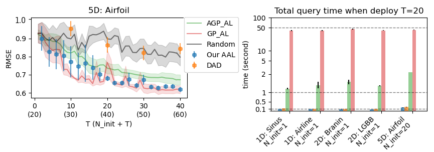
Figure 2: Empirical results on standard AL. RMSE on airfoil dataset as a function of the query points $T$ (left). We deploy our trained policy for various query steps, i.e. $T=2,4,...,40$. For the DAD baseline, an individual policy needs to be trained for each $T$ and we train at snapshots $T=10,20,30,40$. All methods improve performance as the number of queries $T$ increases. Across all datasets, our approach is significantly faster than GP-based methods (right), as deployment involves only a single NN forward pass and no GP modeling or acquisition optimization.

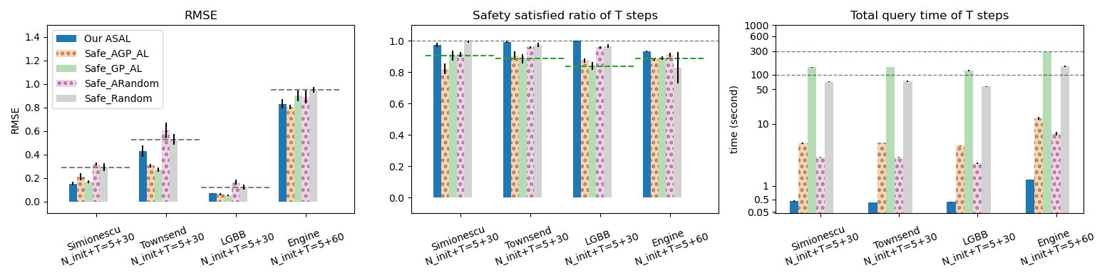
Figure 3: Empirical results on safe AL. Model performance (left): Our approach (blue) performs competitively with other safe AL methods and surpasses the Safe Random baseline across all tasks. The RMSE is evaluated on safe test data only. Safety (middle): Safety awareness is quantified as the proportion of safe queries out of the total $T$ queries. Our method reaches the required safety threshold $1-\gamma$ on all datasets. Runtime (right): Compared to its competitors, our methods refrains from GP modeling and constrained acquisition optimization during querying leading to a significant speed-up. Note that Safe Random is time-consuming as well because a GP is required to estimate the safe set.

In this section, we empirically evaluate our method. We first present unconstrained AL results, demonstrating the effectiveness of our approach in terms of AL exploration. Next, we incorporate safety constraints and show that our approach remains effective in exploration while maintaining safety requirements. All experiments confirm that our methods are well suited for AL tasks that require real-time decision making.

Experimental set-up:

We prepare the experiments by training our neural network policy utilizing Algorithm 2, corresponding to the up-front preparation block in Figure 1. We train one NN policy for each dimensionality $D$ and for each experimental setting (unconstrained, safe). The policies are then applied to all benchmark problems of their respective configuration, corresponding to the deployment block in Figure 1. Our NN policy returns points on continuous space $\mathcal{X}\subseteq\mathbb{R}^{D}$. On benchmark functions, the query $\bm{x}_{t}=\phi(\cdot)$ is used directly for data acquisition. However, for testing on real-world datasets, where only a discrete pool of data points is available, we approximate the query by selecting the nearest point from the pool using the $L2$-norm. Since our high-level goal is to model a regression task, we use the final collected dataset to train a GP model and assess its performance. All experiments report modeling performance, measured with Root Mean Squared Error (RMSE), and AL deployment time. For safe AL, we additionally study if the safety threshold is satisfied. Each AL task is repeated five times with different random seeds and initial data. We provide more experimental details including the training time in Appendix F.

4.1 Unconstrained AL

We first study our approach on standard unconstrained AL tasks, which can be achieved by training on the objective $\mathcal{I}$ (Eq. 5) and removing the safety samples from the generative process in Algorithm 2 (see Appendix Algorithm A.4 for a cleaner version of unconstrained training). We compare our amortized AL (AAL) method against (i) GP AL: AL with a standard GP, GP trained with Type II maximum likelihood (ii) AGP AL: AL with amortized GP (AGP) proposed by Bitzer et al. (2023), where GP hyperparameters are not trained but inferred (iii) Random: random selection criterion and (iv) DAD: amortized Bayesian experimental design proposed by Foster et al. (2021) (Section C.2). We run experiments on 2 benchmark functions and 3 real-world problems: Sin function (dimension $D=1$), Branin function ($D=2$), Airline dataset ($D=1$), Langley Glide-Back Booster dataset (LGBB, $D=2$), and Airfoil dataset ($D=5$).

We report the mean and standard errors on the test dataset in Tables 1 and 2, training loss values in Appendix G. We begin by comparing the model performance: As expected, AL methods generally outperform random sampling, with the exception of the Airline dataset. Among the AL methods, we observe that the performance of AGP sometimes and of DAD often deteriorates (DAD is particularly bad when $D\geq 2$). AGP (Bitzer et al., 2023) infers hyperparameters to approximate Type II maximum likelihood, which might not fully align with the exploration needs of AL tasks. Similarly, DAD is not designed for nonparametric modeling (see Section C.2). Our AAL method, along with the DAD and Random baselines, require GPs only for evaluation purposes. In contrast, GP AL and AGP AL methods rely on GP modeling and acquisition optimization during querying, which significantly increases their runtime compared to our approach (Figure 2).

In summary, our results clearly highlight the advantages of our method on time-sensitive tasks: AAL operates at least an order of magnitude faster than GP-based baselines, while remaining highly effective in exploration.

4.2 Safe AL

In this section, we study safe AL by training on the objective $\mathcal{S}_{\mathcal{H}}$ (Eq. 7) with Algorithm 2. We compare our amortized safe AL (ASAL) against the following baselines: (i) Safe GP AL (Schreiter et al., 2015; Zimmer et al., 2018; Li et al., 2022), which leverages entropy acquisition and standard GP training for the main $f$ and safety function $q$ (Eq. 1), (ii) Safe AGP AL which replaces the standard GP training by AGPs (Bitzer et al., 2023), (iii) Safe Random, where base acquisition scores are random values and a standard GP model estimates the safety values, (iv) Safe ARandom, which replaces the safety GP training by AGP. All methods are deployed with a safety level of $\gamma=0.05$.

Our method builds on the standard safe AL criteria (Eq. 1) with a focus of real-time deployment. Such criteria are usually applied to low-dimensional problems ($D\leq 2$). For higher dimensions, the acquisition optimization problem becomes highly complex and often requires approximations (Kirschner et al., 2019; Bottero et al., 2022). We deploy safe AL on two constrained benchmark functions and two real-world problems: Simionescu function ($D=2$), Townsend function ($D=2$), LGBB dataset ($D=2$) and Engine measurements ($D=3$).

Our main results are shown in Figure 3, with further analyses, including an ablation study on the effect of $\gamma$ and our novel acquisition criterion (Eq. 6) combined with conventional safe AL, presented in Appendix G. ASAL achieves comparable model performance to Safe (A)GP AL on all datasets, except for a slight disadvantage on Townsend, and outperforms Safe (A)Random across the board. It ensures safety awareness, with the proportion of safe queries exceeding the required $1-\gamma$ level on all datasets. Importantly, ASAL is at least an order of magnitude faster than all GP-based methods, including Safe (A)Random, which leverages GPs for safe set estimation. These results highlight the practical advantages of ASAL, offering a versatile solution for safe active learning in real-time applications.

5 Conclusion

We propose an amortized safe AL approach. Our approach leverages GPs to construct a simulator for pretraining the safe AL policy. The trained policy can zero-shot generalize to novel safe AL problems, enabling deployment that (i) queries informative and safe data (ii) eliminates the need for GP modeling and constrained acquisition optimization, resulting in a significant speed-up that facilitiates real-time decision making.

Many existing safe learning methods (Sui et al., 2015; Yanan Sui et al., 2018; Zimmer et al., 2018; Lederer et al., 2021) offer theoretical safety guarantees, which our method does not provide. However, these guarantees typically rely on the assumption of well-chosen GP hyperparameters a priori - an assumption that is rarely met in real-world AL applications.

Our training objectives are based on the GP likelihood, which, in its standard implementation as used here, scales cubically with dataset size. Research into linear solvers for GP training (e.g., Wang et al., 2019) offers potential alternatives to overcome this limitation. This, along with amortizable batch selection strategies (Citovsky et al., 2021), represents an active area for future research.

Future work could also extend our approach to support flexible input dimensions, as currently, a new NN policy is required for each distinct number of input features.

Appendix

Appendix A Gaussian Process: Distribution and Entropy

GP distribution:

We first write down the GP predictive distribution. Details can be seen in Rasmussen & Williams (2006). We write down a general form with a non-zero prior mean $q\sim\mathcal{GP}(\mu_{q},k_{q})$. The GP hyperparameters are omitted for brevity. One can remove $\mu_{q}$ to get a zero-mean GP distribution, e.g. for $y$.

Given a set of $N_{\text{observe}}$ data points $\mathcal{D}=\{\bm{X},Z\}\subseteq\mathcal{X}\times\mathcal{Z}$, we wish to make inference at points $\bm{X}_{\text{test}}=\{\bm{x}_{\text{test},1},...,\bm{x}_{\text{test},N_{\text{test}}}\}$. We write $Z_{\text{test}}=(z(\bm{x}_{\text{test},1}),...,z(\bm{x}_{\text{test},N_{\text{test}}}))$ for brevity. The joint distribution of $Z$ and predictive $Z_{\text{test}}$ is Gaussian:

$$\begin{split}p(Z,Z_{\text{test}})=\mathcal{N}\left(\mu_{q}(\bm{X}\cup\bm{X}_{\text{test}}),k_{q}(\bm{X}\cup\bm{X}_{\text{test}},\bm{X}\cup\bm{X}_{\text{test}})+\sigma_{q}^{2}I_{N_{\text{observe}}+N_{\text{test}}}\right)\end{split}$$ (A.8)

where $k_{q}(\bm{X}\cup\bm{X}_{\text{test}},\bm{X}\cup\bm{X}_{\text{test}})$ is a gram matrix with $[k_{q}(\bm{X}\cup\bm{X}_{\text{test}},\bm{X}\cup\bm{X}_{\text{test}})]_{i,j}=k_{q}\left([\bm{X}\cup\bm{X}_{\text{test}}]_{i},[\bm{X}\cup\bm{X}_{\text{test}}]_{j}\right)$.

This leads to the following predictive distribution (or GP posterior distribution)

$$\begin{split}p(Z_{\text{test}}|Z)&=\mathcal{N}\left(Z_{\text{test}}|\mu_{\mathcal{D}}(\bm{X}_{\text{test}}),cov_{\mathcal{D}}(\bm{X}_{\text{test}})\right),\\ \mu_{\mathcal{D}}(\bm{X}_{\text{test}})&=k_{q}\left(\bm{X}_{\text{test}},\bm{X}\right)\left[k_{q}\left(\bm{X},\bm{X}\right)+\sigma_{q}^{2}I_{N_{\text{observe}}}\right]^{-1}\left[Z-\mu_{q}\left(\bm{X}\right)\right]+\mu_{q}\left(\bm{X}_{\text{test}}\right),\\ cov_{\mathcal{D}}(\bm{X}_{\text{test}})&=k_{q}\left(\bm{X}_{\text{test}},\bm{X}_{\text{test}}\right)+\sigma_{q}^{2}I_{N_{\text{test}}}\\ &-k_{q}\left(\bm{X}_{\text{test}},\bm{X}\right)\left[k_{q}\left(\bm{X},\bm{X}\right)+\sigma_{q}^{2}I_{N_{\text{observe}}}\right]^{-1}k_{q}\left(\bm{X},\bm{X}_{\text{test}}\right).\end{split}$$ (A.9)

Elements of the predictive mean vector $\mu_{\mathcal{D}}(\bm{X}_{\text{test}})$ are the noise-free predictive function values.

Inverting a $N_{\text{observe}}\times N_{\text{observe}}$ matrix $\left[k_{q}\left(\bm{X},\bm{X}\right)+\sigma_{q}^{2}I_{N_{\text{observe}}}\right]$ has complexity $\mathcal{O}(N_{\text{observe}}^{3})$ in time.

When a GP is used to model the probability beyond a threshold, e.g. a predictive safety probability, at a test point $\bm{x}$ this is a cumulative distribution function

$$\begin{split}p(z(\bm{x})\geq 0|Z)=1-p(z(\bm{x})<0|Z)=&1/2\left[1+erf\left(\frac{\mu_{\mathcal{D}}(\bm{x})}{\sqrt{2cov_{\mathcal{D}}(\bm{x})}}\right)\right].\end{split}$$ (A.10)

The log probability density function is

$$\begin{split}\log p(Z_{\text{test}}|Z)=&-n/2\log(2\pi)-1/2\log\det(cov_{\mathcal{D}}(\bm{X}_{\text{test}}))\\ &-{\color[rgb]{0,0,1}1/2(Z_{\text{test}}-\mu_{D}(\bm{X}_{\text{test}}))^{T}\left[cov_{\mathcal{D}}(\bm{X}_{\text{test}})\right]^{-1}(Z_{\text{test}}-\mu_{D}(\bm{X}_{\text{test}}))},\end{split}$$ (A.11)

inverting $cov_{\mathcal{D}}(\bm{X}_{\text{test}})$ or computing the determinant takes $\mathcal{O}(N_{\text{test}}^{3})$ in time.

GP entropy:

If we consider $Z_{\text{test}}$ as a collection of $N_{\text{test}}$ random variables, the entropy is

$$\mathbb{H}(Z_{\text{test}}|Z)= \mathbb{E}_{p(Z_{\text{test}}|Z)}[-\log p(Z_{\text{test}}|Z)]=n/2\log(2\pi{\color[rgb]{0,0,1}e})+1/2\log\det(cov_{\mathcal{D}}(\bm{X}_{\text{test}})).$$ (A.12)

The difference between $-\log p(\cdot)$ and $\mathbb{H}(\cdot)$ is marked blue, and this comparison will be described later when we look into different training objectives. Note further that if we plug predicted function values $Z_{\text{test}}=\mu_{D}(\bm{X}_{\text{test}})$ into Eq. A.11, then the blue term becomes zero and this becomes proportional to negative entropy.

GP training:

When we deploy a conventional (safe) AL, or when we use the collected data after a deployment to model a function, we usually need to select the hyperparameters. One standard approach is to conduct a Type II maximum likelihood:

$$\text{argmax}_{\theta_{q},\sigma^{2}}\log p(Z|\bm{X})=\text{argmax}_{\theta_{q},\sigma^{2}}\log\mathcal{N}\left(Z|\mu_{q}(\bm{X}),k_{q}(\bm{X},\bm{X})+\sigma^{2}I_{N_{\text{observe}}}\right),$$

where the free variables are hyperparameters of $\mu_{q},k_{q}$. The time complexity is $\mathcal{O}\left(N_{\text{observe}}^{3}\right)$ while the exact factor depends on the number of parameters, the optimizer, and the numerical stability. We keep the prior mean $\mu_{q}$ for consistent notation even though the only place when we train GPs is during deployment where we use zero mean GPs.

Appendix B Policy NN Structure

,

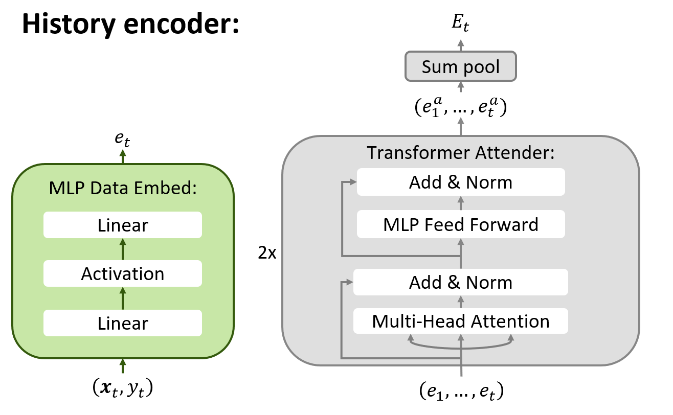
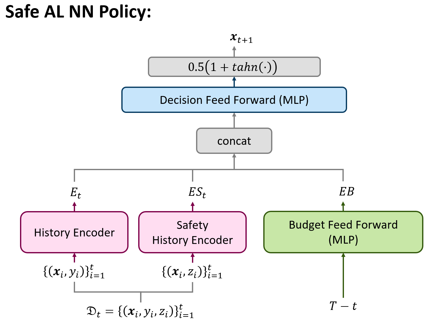
Figure A.B.4: Our NN $\phi(T-t,\mathcal{D}_{t})=\bm{x}_{t+1}$. Each observation pair $(\bm{x}_{t},y_{t})$ (or $(\bm{x}_{t},z_{t})$) is first mapped by an MLP to an embedding $e_{t}$. Data of different $t$ use the same MLP Data Embed module, i.e. one history encoder has only one MLP Data Embed. A sequence of data embeddings is then stacked and attended by a $2$-layer transformer encoder (Vaswani et al., 2017), and then a final history embedding is obtained by summing up the attended per-data embeddings $\sum_{t}e_{t}^{a}$. The sum pool ensures an invariance of input data order. Details of the history encoder are described in Foster et al. (2021); Ivanova et al. (2021). The history encoder and safety history encoder are two modules of individual parameters. The budget variable is as well mapped by a separate MLP module to a budget embedding $EB$. The history embedding $E_{t}$, safety history embedding $ES_{t}$, and the budget embedding $EB$ are stacked, mapped by another MLP module, and then refrained by a $tahn$ function to a bounded input domain $[0,1]^{D}$.

We build our NN upon the structure described in Foster et al. (2021); Ivanova et al. (2021). The final structure is sketched in Figure A.B.4. We summarize the comparison between our network and the one developed by Ivanova et al. (2021):

1. the history encoder ($\{(\bm{x}_{i},y_{i})\}_{i=1}^{t}\rightarrow E_{t}$) and the decision feed forward MLP (originally $E_{t}\rightarrow\bm{x}_{t+1}$) are taken from Ivanova et al. (2021);

2. we add a hyperbolic tangent function as the last layer to ensure the policy output is in our bounded $\mathcal{X}$, which was not needed in the original Bayesian experimental design problems;

3. we add another history encoder to handle the safety data;

4. we add a budget encoder to handle the budget variable.

Our NN structure is highly modularized. The safety history encoder can be removed to form a budget-aware unconstrained AL policy. If we intend to work on a policy under fixed budget, i.e. $T_{\text{sim}}$ is fixed to $T$ in Algorithm 2, we can remove the Budget Feed Forward module.

Appendix C Training Objectives: Details, Illustrations, More Objectives

In this section, we provide

• an illustration of our entropy objective, another version of our entropy objective and an illustration (Section C.1),

• details of our regularized entropy (mutual information) objective, another version of our regularized entropy objective (Section C.1),

• details of the DAD baseline in our GP context (Section C.2),

• an illustration of our safe AL objective, an additional safe AL objective and an illustration (Section C.3).

This section inherits the notation of Section 3.1. The objectives are computed with simulated (safe) AL instances.

C.1 Objectives: Unconstrained AL

In this section, we provide an illustration of our main unconstrained AL entropy objective, details of our regularized entropy, and additional objectives.

Note first that our unconstrained AL training does not need the safety measurements: a NN may have no safety history encoder (Figure A.B.4), and the training algorithm can operate with neither safety measurements $q$ and $z$ nor safety center $\mathcal{C}$. Therefore, our main safe AL training (Algorithm 2) can be reduced to Algorithm A.4.

Algorithm A.4 Unconstrained AL Policy Training

0: 2.1, $T$, $N_{\text{init}}$

1: sample a batch of $(\theta,\sigma^{2})$

2: sample a batch of $(f,\mathcal{D}_{0})$ per Algorithm A.5

3: for each $(f,\mathcal{D}_{0})$ do

4:  sample $T_{\text{sim}}\sim\text{Uniform}[1,T]$

5:  for $t=1,...,T_{\text{sim}}$ do

6:   $\bm{x}_{\phi,t}=\phi(T_{\text{sim}}-t+1,\mathcal{D}_{t-1})$

7:   sample $\epsilon_{t}\sim\mathcal{N}(0,\sigma^{2}),y_{\phi,t}=f(\bm{x}_{\phi,t})+\epsilon_{t}$

8:   $\mathcal{D}_{t}\leftarrow\mathcal{D}_{t-1}\cup\{\bm{x}_{\phi,t},y_{\phi,t}\}$

9:  end for

10: end for

11: compute AL loss (e.g. Eq. 5), update $\phi$

Algorithm A.5 Unconstrained Initial Sampling

0: 2.1, $N_{\text{init}}$, $\mathcal{GP}(0,k_{\theta}),\sigma^{2}$

1: sample $f_{0}\sim\mathcal{GP}(0,k_{\theta})$

2: $f(\cdot)=f_{0}(\cdot)-\mathbb{E}_{\bm{x}\in\mathcal{X}}[f_{0}(\bm{x})]$

3: sample $\bm{X}_{\text{init}}\sim\text{Uniform}[\mathcal{X}],|\bm{X}_{\text{init}}|=N_{\text{init}}$

4: sample $\mathcal{E}_{\text{init}}\sim\mathcal{N}(0,\sigma^{2}I)$

5: $Y_{\text{init}}=f(\bm{X}_{\text{init}})+\mathcal{E}_{\text{init}}$

6: $\mathcal{D}_{0}=\{\bm{X}_{\text{init}},Y_{\text{init}}\}$

7: return $f,\mathcal{D}_{0}$

C.1.1 Objectives: Unconstrained AL - Entropy

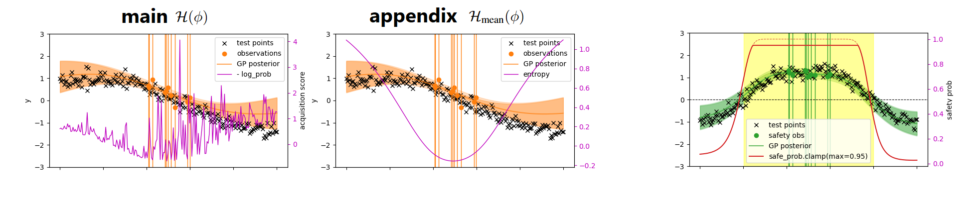
Figure A.C.5: Simulated unconstrained AL objectives and safety probability. $T_{\text{sim}}=1$. Given observed data ($y$ orange, $z$ green), we plot GP posteriors (orange, Eq. A.9), compute AL objectives (pink) and the safety likelihood $p(z(\cdot)\geq 0|z_{\text{observed}})$ (red, Eq. A.10) of the next queries (black). The yellow region is the true safe area. The objectives illustrated are meant to be maximized. Note that $y,z$ are available because our training scheme simulates AL before utilizing the evaluations for objective computations. A conventional (safe) AL optimizes queries based on inferred future evaluations.

Here, we illustrate our main entropy objective, and we introduce another version of the entropy objective.

In our main paper, we introduce the unconstrained AL meta objective

$$\mathcal{H}(\phi)\propto \mathbb{E}_{\theta,\sigma^{2}}\mathbb{E}_{f,T_{\text{sim}},\mathcal{E}_{\text{init}},\epsilon_{1:T_{\text{sim}}}}\left[\frac{-\log p(y_{\phi,1},...,y_{\phi,T_{\text{sim}}}|Y_{\text{init}})}{N_{\text{init}}+T_{\text{sim}}}\right]~\text{(\lx@cref{creftypeplural~refnum}{eq-gp_logprob_objective} and\nobreakspace\lx@cref{refnum}{eq-gp_logprob_objective_inner})}.$$

Here, we introduce another objective function which computes

$$\mathcal{H}_{\text{mean}}(\phi) =\mathbb{E}_{\theta,\sigma^{2}}\mathbb{E}_{f,T_{\text{sim}},\mathcal{E}_{\text{init}},\epsilon_{1:T_{\text{sim}}}}\left[\frac{\mathbb{H}(y(\bm{x}_{\phi,1}),...,y(\bm{x}_{\phi,T_{\text{sim}}})|Y_{\text{init}})}{N_{\text{init}}+T_{\text{sim}}}\right].$$ (A.13)

Note that entropy $\mathbb{H}$ takes random variables, not the sampled $y_{\phi,1},...,y_{\phi,T_{\text{sim}}}$. Substituting Eqs. A.11 and A.12 into the objectives, we see that the key difference (marked blue) is indeed whether the observation values $y_{\phi,1},...,y_{\phi,T}$ are taken into account. Our main $\mathcal{H}$ aims for points $y_{\phi,1},...,y_{\phi,T}$ that are the most distinctive, while $\mathcal{H}_{\text{mean}}$ aims for $\bm{x}_{\phi,1},...,\bm{x}_{\phi,T}$ that have the most uncertainty jointly (no actual function values). We suspect that having $y_{\phi,1},...,y_{\phi,T}$ in the loss (our main $\mathcal{H}$, Eq. 4) may help the policy adapt in an AL deployment. Please see Figure A.C.5 for illustrations. One can see that $\mathcal{H}$ has the evaluated $y_{\phi,1:T_{\text{sim}}}$ which encodes actual function values and noises.

The subscript name is ”mean” because $\mathbb{H}$ computes the expectation of negative log likelihood.

Note that, if we would obtain each $\bm{x}_{\phi,t+1}$ step-wise, the objectives $\mathcal{H},\mathcal{H}_{\text{mean}}$ correspond to the following acquisition function:

$$\begin{split}a_{\mathcal{H}}(\bm{x}|y_{\phi,1:t},Y_{\text{init}})&=-\log p(\hat{y}(\bm{x})|y_{\phi,1:t},Y_{\text{init}}),\\ a_{\mathcal{H}_{\text{mean}}}(\bm{x}|y_{\phi,1:t},Y_{\text{init}})&=\mathbb{E}_{y(\bm{x})|y_{\phi,1:t},Y_{\text{init}}}\left[-\log p(y(\bm{x})|y_{\phi,1:t},Y_{\text{init}})\right]\\ &=\mathbb{H}(y(\bm{x})|y_{\phi,1:t},Y_{\text{init}}).\end{split}$$ (A.14)

Here, $y(\bm{x})$ is a random variable forecasting into the next query, while $\hat{y}(\bm{x})$ is an estimated value. In a conventional scenario where the acquisition function measures the unqueried future point, one may take the GP predictive mean for $\hat{y}(\bm{x})$ resulting in $a_{\mathcal{H}}(\bm{x}|y_{\phi,1:t},Y_{\text{init}})=-1/2\log e+\mathbb{H}(y(\bm{x})|y_{\phi,1:t},Y_{\text{init}})\propto\mathbb{H}(y(\bm{x})|y_{\phi,1:t},Y_{\text{init}})$ (Eqs. A.9, A.11 and A.12). In our simulation, $\hat{y}(\bm{x})$ would be the simulated noisy function realization (not just at $\bm{x}_{\phi,t}$ but all $\bm{x}\in\mathcal{X}$) where $\hat{y}(\bm{x}_{\phi,t+1})=y_{\phi,t+1}$.

$\mathbb{H}(y(\bm{x})|y_{\phi,1:t},Y_{\text{init}})$ is the standard predictive entropy (Seo et al., 2000; Krause & Guestrin, 2007).

We refer the readers to Krause & Guestrin (2007); Krause et al. (2008) for detailed discussions of conventional GP AL methods. In these papers, the authors discuss sequential step-wise querying and joint batch querying. Our training scheme can be considered as a special case where the policy performs sequential querying while the objectives compute joint batch querying but with true evaluations.

C.1.2 Objectives: Unconstrained AL - Regularized Entropy

Here, we discuss empirical issues of unconstrained entropy and our approach using mutual information objectives (Guestrin et al., 2005; Krause et al., 2008).

Maximizing an entropy objective favors a set of distinctive points, which naturally encourages points at the border, as they are the most scattered. Guestrin et al. (2005) argued that exploring the border may be suboptimal because we would rather explore inside the space. The authors further proposed a mutual information acquisition criterion to tackle this problem, at least in conventional AL settings. In our training scheme, the objectives $\mathcal{H}(\phi)$ and $\mathcal{H}_{\text{mean}}(\phi)$ sometimes overemphasize the border and completely ignore the inner region of $\mathcal{X}$, which is clearly not desired. Part of the reasons can be the tanh layer in our NN (Figure A.B.4), which, although helping us bound the NN outputs in $\mathcal{X}$, has vanishing gradients at the boundary. To tackle this issue, we wish to derive a mutual information objective suitable for our framework.

In active GP learning, Guestrin et al. (2005) define a mutual information criterion as the reduction of entropy in an unexplored region: $\mathbb{H}(y(\bm{x}_{\phi,1}),...,y(\bm{x}_{\phi,T})|Y_{\text{init}})-\mathbb{H}(y(\bm{x}_{\phi,1}),...,y(\bm{x}_{\phi,T})|Y_{\text{init}},y(\mathcal{X}\setminus\bm{X}_{\phi}))$, $y(\mathcal{X}\setminus\bm{X}_{\phi})$ means the outputs corresponding to $\mathcal{X}\setminus\{\bm{x}_{\phi,1},...,\bm{x}_{\phi,T}\}$. The original paper considered small discrete $\mathcal{X}$ where $y(\mathcal{X}\setminus\{\bm{x}_{\phi,1},...,\bm{x}_{\phi,T}\})$ is a computable set of random variables. In our framework, $\mathcal{X}$ is a continuous space, and thus this is not well-defined. Even if $\mathcal{X}$ is discrete, conditioning on a large pool (fine discretization) is computationally heavy, i.e. GP cubic complexity $\mathcal{O}\left(|\mathcal{X}|^{3}\right)$ (Appendix A). A discrete pool also enforces a classifier-like policy $\phi$, as the policy needs to select points from a pool, which prohibits us from utilizing the current NN structure developed on top of Foster et al. (2021); Ivanova et al. (2021).

To derive mutual information objectives suitable for our learning framework, note that entropy reduction is a regularized entropy objective. We propose a simple yet effective approach: compute the regularization term only on a sparse set of $N_{\text{grid}}$ samples $\left(\bm{X}_{\text{grid}},Y_{\text{grid}}\right)\subseteq\mathcal{X}\times\mathcal{Y}$. Then we turn the acquisition functions proposed by Guestrin et al. (2005); Krause & Guestrin (2007) into the following training objectives

$$\begin{split}\mathcal{I}(\phi)=&\mathbb{E}_{\theta,\sigma^{2}}\mathbb{E}_{f,T_{\text{sim}},\mathcal{E}_{\text{init}},\epsilon_{1:T_{\text{sim}}}}\left[\frac{-\log p(y_{\phi,1:T_{\text{sim}}}|Y_{\text{init}})+\log p(y_{\phi,1:T_{\text{sim}}}|Y_{\text{init}},Y_{\text{grid}})}{N_{\text{init}}+T_{\text{sim}}}\right]~\text{(\lx@cref{creftypeplural~refnum}{eq-gp_logprob_reduction_objective} and\nobreakspace\lx@cref{refnum}{eq-gp_logprob_reduction_objective_inner})},\end{split}$$

$$\begin{split}\mathcal{I}_{\text{mean}}(\phi)=&\mathbb{E}_{\theta,\sigma^{2}}\mathbb{E}_{f,T_{\text{sim}},\mathcal{E}_{\text{init}},\epsilon_{1:T_{\text{sim}}}}\left[\frac{\mathbb{H}(y(\bm{x}_{\phi,1:T_{\text{sim}}})|Y_{\text{init}})-\mathbb{H}(y(\bm{x}_{\phi,1:T_{\text{sim}}})|Y_{\text{init}},Y_{\text{grid}})}{N_{\text{init}}+T_{\text{sim}}}\right].\end{split}$$ (A.15)

$N_{\text{grid}}$ should be much larger than $T$. Maximizing these objectives encourages $\{\bm{x}_{\phi,1},...,\bm{x}_{\phi,T}\}$ to track subsets of $\bm{X}_{\text{grid}}$. The intuition is two-fold: (i) we can view them as entropy objectives regularized by an additional search space indicator, or (ii) we can view them as imitation objectives because a subset of grid points, if happens to have small joint likelihood or large joint entropy, maximizes the objective.

Note that, to keep the policy from overfitting those sparse grid samples, which are not necessarily optimal points, we re-sample $\bm{X}_{\text{grid}}$ in each training step. We sample $\bm{X}_{\text{grid}}$ with $\text{Beta}(0.5,0.5)$, but a uniform distribution can also be used and we did not see obvious difference. Empirically, training with the two mutual information objectives are easier to converge than the entropy objectives. Entropy objectives often stick in border-only patterns, particularly when $D\geq 2$.

One drawback of such objectives is that we lack insight into the appropriate number of the grid points. When the dimension of $\mathcal{X}$ grows, $N_{\text{grid}}$ might need to be increased, which can make our mutual information objectives computationally impossible. We provide our exact $N_{\text{grid}}$ in Table A.E.2.

Our ablation study in Appendix G demonstrate the results of $\mathcal{I}_{\text{mean}}$.

Note that this regularization is meaningless to safe AL, because the border of $\mathcal{X}$ is typically less safe and the safe AL objectives already reflect this (Figure A.C.6)

C.2 Objectives: DAD Baseline

Algorithm A.6 DAD Training with GP Prior

0: 2.1, $T$, $N_{\text{init}}$

1: sample a batch of $(\theta,\sigma^{2})$

2: for each $(\theta,\sigma^{2})$ do

3:  sample $f_{0,\text{raw}}\sim\mathcal{GP}(0,k_{\theta})$

4:  $f_{0}(\cdot)=f_{0,\text{raw}}(\cdot)-\mathbb{E}_{\bm{x}\in\mathcal{X}}[f_{0,\text{raw}}(\bm{x})]$

5:  sample $\bm{X}_{\text{init}}\sim\text{Uniform}[\mathcal{X}],|\bm{X}_{\text{init}}|=N_{\text{init}}$

6:  sample $\mathcal{E}_{\text{init}}\sim\mathcal{N}(0,\sigma^{2}I),Y_{\text{init}}=f_{0}(\bm{X}_{\text{init}})+\mathcal{E}_{\text{init}}$

7:  $\mathcal{D}_{0}=\{\bm{X}_{\text{init}},Y_{\text{init}}\}$

8:  for $t=1,...,T$ do

9:   $\bm{x}_{\phi,t}=\phi(\mathcal{D}_{t-1})$

10:   sample $\epsilon_{t}\sim\mathcal{N}(0,\sigma^{2}),y_{\phi,t}=f_{0}(\bm{x}_{\phi,t})+\epsilon_{t}$

11:   $\mathcal{D}_{t}\leftarrow\mathcal{D}_{t-1}\cup\{\bm{x}_{\phi,t},y_{\phi,t}\}$

12:  end for

13:  sample $f_{l,\text{raw}}\sim\mathcal{GP}(0,k_{\theta}),l=1,...,N_{f,q}$

14:  $f_{l}(\cdot)=f_{l,\text{raw}}(\cdot)-\mathbb{E}_{\bm{x}\in\mathcal{X}}[f_{l,\text{raw}}(\bm{x})],l=1,...,N_{f,q}$

15: end for

16: compute DAD loss (Eq. A.16), update $\phi$

We describe the DAD baseline in our GP context (Foster et al., 2021). DAD is a scheme which samples tasks and learns to perform Bayesian optimal experimental design originally aiming at parametric models. Bayesian optimal experimental design aims to query data to learn about a posterior Bayesian model (Rainforth et al., 2024). In a GP learning problem, this means collecting $\bm{x}_{1:T},y_{1:T}$ to make inference $p(f(\cdot)|\bm{X}_{\text{init}},Y_{\text{init}},\bm{x}_{1:T},y_{1:T})$. DAD follows similar training procedure: we (i) sample tasks from a prior, and (ii) learn a data querying policy by optimizing the DAD objective. To train with DAD, one may use our main training algorithm because we generate more quantities than needed by the DAD objective. For clarity, however, we write down a clean version of DAD training in Algorithm A.6, which is the Algorithm 1 of Foster et al. (2021) combined with our GP prior. We summarize the comparison between DAD and our main safe AL training (Algorithm 2): (i) safety measurements are not present in DAD, (ii) the policy of DAD does not take the budget variable while $T_{\text{sim}}=T$ is fixed during the training, and (iii) functions $f_{0},...,f_{N_{f,q}}$ are sampled but the DAD objective simulates the observations $Y_{\text{init}},y_{1:T}$ on $f_{0}$ only while $f_{1},...,f_{N_{f,q}}$ are contrastive samples for noise contrastive estimations. Note that in this paper, $N_{f,q}$ denotes the number of functions $|\{(f,q)\}|$ per set of GP hyperparameters. Here, we use $N_{f,q}$ to denote the number of contrastive functions.

The objective is

$$DAD(\phi)=\mathbb{E}_{\theta,\sigma^{2}}\left[\mathbb{E}_{f_{0},...,f_{N_{f,q}},\mathcal{E}_{\text{init}},\epsilon_{1:T}}\left[\log\frac{p(Y_{\text{init}},y_{\phi,1:T}|f_{0})}{1/(N_{f,q}+1)\sum_{l=0}^{N_{f,q}}p(Y_{\text{init}},y_{\phi,1:T}|f_{l})}\right]\right].$$ (A.16)

This objective is meant to be maximized.

This objective was derived for parametric models, i.e. $p(\text{model parameters}|\text{data})$ in contrast to our $p(f|\text{data})$. Please see Foster et al. (2021) for details.

Notice that a further work, Ivanova et al. (2021), extended DAD to more general scenarios, for example, allowing intractable $p(y|f)$. However, their proposed learning objectives require another NN mapping, $\{(\mathcal{D},f)\}\rightarrow\mathbb{R}$ if described in our notation, to help estimate the involved intractable distributions. Such a mapping is not applicable for nonparametric $f$, and the objectives in Ivanova et al. (2021) were again not designed for AL of nonparametric functions. This is a different direction to what we need in this paper.

C.3 Objectives: Safe AL

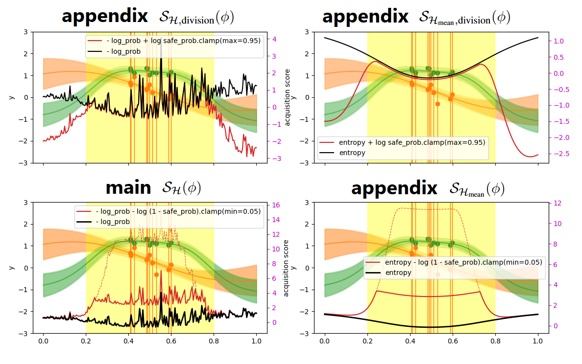
Figure A.C.6: Simulated safe AL objectives. $T_{\text{sim}}=1$. As described in Figure A.C.5, orange and green are $y,z$ and the corresponding GP predictions, while black curves are unconstrained objectives $\mathcal{H},\mathcal{H}_{\text{mean}}$. Our safe AL objectives (red) decorate the unconstrained objectives with our main min unsafe log probability (bottom, $\mathcal{S}_{\cdot}$, Eq. 7) or with the appendix max safe log probability (top, $\mathcal{S}_{\cdot,\text{division}}$, Eq. A.17). The objectives illustrated are meant to be maximized. Red dashed lines show the objectives if the safety probability is not clamped by $\gamma$. Note again that $y,z$ are available because our training scheme simulates AL before utilizing the evaluations for objective computations.

We illustrate our main safe AL objective, and we introduce more objectives.

In our main paper, we propose a safe AL objective

$$\mathcal{S_{H}}(\phi) =\mathbb{E}\left[\frac{-\log p(y_{\phi,1},...,y_{\phi,T_{\text{sim}}}|Y_{\text{init}})-\sum_{t=0}^{T_{\text{sim}}-1}\log\ \text{max}(\gamma,p(z(\bm{x}_{\phi,t+1})<0|z_{\phi,1:t},Z_{\text{init}}))}{N_{\text{init}}+T_{\text{sim}}}\right]~\text{(\lx@cref{creftype~refnum}{eq-safe_gp_logprob_objective})}.$$

This objective is a combination of an unconstrained exploration objective and a safety regularization. We are able to exchange the exploration term $-\log p(y_{\phi,1},...,y_{\phi,T_{\text{sim}}}|Y_{\text{init}})$ by any other objectives, e.g. $\mathcal{S}_{\mathcal{H}_{\text{mean}}}(\phi)$ corresponds to safety decorated $\mathcal{H}_{\text{mean}}(\phi)$.

If we take a closer look into the safety term, the objective is maximized when $\log p(z(\bm{x}_{\phi,t+1})<0|z_{\phi,1:t},Z_{\text{init}})$ is small. Ideally, the probability of being unsafe should be small (or equivalently the probability of being safe is large, Figure A.C.5). Minimizing the unsafe probability nevertheless makes the $\log$ value explode to negative infinity (if not clamped by a non-zero $\gamma$). Numerically, we suggest to add a small number to the probability to stabilize the computations; e.g., we add $10^{-5}$ for clamped and non-clamped versions for stability.

Nevertheless, another approach we consider is to change the safety term, so that we directly maximize the safety probability

$$\begin{split}&-\log p(y_{\phi,1},...,y_{\phi,T_{\text{sim}}}|Y_{\text{init}})+\sum_{t=0}^{T_{\text{sim}}-1}\log p(z(\bm{x}_{\phi,t+1})\geq 0|z_{\phi,1:t},Z_{\text{init}})\\ =&-\sum_{t=0}^{T_{\text{sim}}-1}\log\frac{p(y_{\phi,t+1}|y_{\phi,1:t},Y_{\text{init}})}{p(z(\bm{x}_{\phi,t+1})\geq 0|z_{\phi,1:t},Z_{\text{init}})},\end{split}$$

which corresponds to

$$\mathcal{S}_{\mathcal{H},\text{division}}(\phi) =\mathbb{E}\left[\frac{-\log p(y_{\phi,1},...,y_{\phi,T_{\text{sim}}}|Y_{\text{init}})+\sum_{t=0}^{T_{\text{sim}}-1}\log p(z(\bm{x}_{\phi,t+1})\geq 0|z_{\phi,1:t},Z_{\text{init}})}{N_{\text{init}}+T_{\text{sim}}}\right].$$ (A.17)

Note that $z(\bm{x}_{\phi,t+1})$ is a prediction, not the evaluated $z_{\phi,t+1}$. Similarly, we may exchange the base exploration term to get e.g. $\mathcal{S}_{\mathcal{H}_{\text{mean}},\text{division}}(\phi)$. With this objective, we do not clamp the safety probability with $\gamma$ because this has no visible effect (see Figure A.C.6). The reason is, if we would clamp the likelihood, i.e. $\text{min}(1-\gamma,p(z(\bm{x}_{\phi,t+1})\geq 0|z_{\phi,1:t},Z_{\text{init}})$ (maximizing the safety likelihood until $1-\gamma$), then the clamped term is optimized towards $p(z(\bm{x}_{\phi,t+1})\geq 0|z_{\phi,1:t},Z_{\text{init}})\geq 1-\gamma$ but for small $\gamma$, $\log(1-\gamma)\approx\log 1$.

Please see Figure A.C.6 for an illustration. Our main $\mathcal{S}_{\cdot}$ is more conservative at the safe set border while the appendix $\mathcal{S}_{\cdot,\text{division}}$ is more prone to space exploration.

In this paper, we avoid coupling $\mathcal{I},\mathcal{I}_{\text{mean}}$ with our safety terms because (i) it is rather tricky to sample $\{\bm{X}_{\text{grid}},Y_{\text{grid}},Z_{\text{grid}}\}$ (Eqs. A.15 and 5) when a safety constraint is present, (ii) we do not see an obvious intuition behind such safe AL objectives, and (iii) we do not see empirical benefit in our preliminary experiments (not shown in the paper).

We illustrate the safe AL objectives in Figure A.C.6 for $T_{\text{sim}}=1$.

Appendix D Training: GP Function Sampling

This section outlines the mathematical details of our GP function sampling, i.e. Algorithm 3.

We first introduce our GP kernel. In our paper, we always use an RBF kernel, including $k_{\theta},k_{q}$ in Algorithm 3 and the GP kernel in benchmark experiments. An RBF kernel has $D+1$ variables: the variance $v$ and a $D$ dimension lengthscale vector $\bm{l}=(l_{1},...,l_{D})$

$$k(\bm{x},\bm{x}^{\prime})=v\exp\left(-1/2\sum_{d=1}^{D}\left(\frac{[\bm{x}-\bm{x}^{\prime}]_{d}}{l_{d}}\right)^{2}\right).$$ (A.18)

D.1 Fourier Feature Functions

In Algorithm 3, the GP functions $f_{0}\sim\mathcal{GP}(0,k_{\theta}),q_{0}\sim\mathcal{GP}(0,k_{q})$ are approximated by Fourier features, which means each function sample is a linear combination of cosine functions (Rahimi & Recht, 2007; Wilson et al., 2020):

$$\text{e.g. }f_{0}(\bm{x})=\sum_{i=1}^{L}\omega_{i}\sqrt{2/L}\cos\left(\bm{a}_{i}^{T}\bm{x}+b_{i}\right),$$

$\omega_{i}\sim\mathcal{N}(0,\sqrt{v}^{2}),\bm{a}_{i}\sim\mathcal{N}(0,\text{diag}\{\bm{l}\}^{-1})$ are kernel dependent and $b_{i}\sim\text{Uniform}(0,2\pi)$. Each function has $L*(D+2)$ parameters. Larger $L$ lead to better approximations. An error bound w.r.t. $D$ and $L$ can be seen in Rahimi & Recht (2007). We set $L=100$.

Remark D.1 (running out of symbols).

We highlight that the parameters of our Fourier feature functions, $\omega_{i},\bm{a}_{i}$ and $b_{i}$, are independent of our acquisition function notation $a(\cdot)$ or other constants. The Fourier feature function parameters (except for $L$, the number of features) are used only for this subsection and will not be referred in any other part of the paper.

In our main paper, the analytical mean of window $\mathcal{X}=[0,1]^{D}$ is computed such that all functions can be shifted to zero mean in the particular domain. The analytical mean is the integral of $f_{0}(\bm{x}),q_{0}(\bm{x})$ divided by volume of $[0,1]^{D}$. We give examples for the one and two dimensional cases:

$$\sum_{i=1}^{L}\frac{1}{a_{i}}\omega_{i}\sqrt{2/L} \sin\left(a_{i}x+b_{i}\right)|_{x=0}^{1}\text{, for }D=1,$$

$$\sum_{i=1}^{L}\frac{-1}{[\bm{a}_{i}]_{1}[\bm{a}_{i}]_{2}}\omega_{i}\sqrt{2/L} \cos\left([\bm{a}_{i}]_{1}x_{1}+[\bm{a}_{i}]_{2}x_{2}+b_{i}\right)|_{x_{1}=0}^{1}|_{x_{2}=0}^{1}\text{, for }D=2,$$

higher dimensions are analogous.

It may happen that at least one component of $\bm{a}_{i}$ is zero or is close to zero, which causes a problem in the division. In this case, we replace $|1/\prod_{d=1}^{D}[\bm{a}_{i}]_{d}|$ by $100000$. The error is negligible, i.e. much smaller than noise level. We can replace $[0,1]^{D}$ by any windows of our interest.

The complexity of computing such mean is $\mathcal{O}\left(L2^{D}\right)$, and this can be distributed to time or space. With common GP and RBF kernel dimensions, e.g. $D\leq 10$, this complexity is negligible.

D.2 Prior Mean of Safety Functions

Figure A.D.7: Examples of sampled $q\sim\mathcal{GP}\left(\mu_{q},k_{q}\right)$. We run Algorithm 3 to sample $f$ (not shown) and $q$. The observations are blurred with noises. The top are five samples of $z\left([0,1]^{2}\right)$, the bottom safe and unsafe classifications $z\left([0,1]^{2}\right)\geq 0$. Black dots are the sampled initial data. The parameters of $\mu_{q},k_{q}$ leverage samplers listed in Table A.F.4. Our algorithm samples diverse safety patterns while guaranteeing stable initial safe data sampling.

As described in our main Section 3.2, we use a GP mean function $\mu_{q}$ to help us control the safety function sampling.

The overall goal is to sample functions $q\sim\mathcal{GP}_{\theta_{q}}(\mu_{q},k_{q})$, while guaranteeing a high probability of the existence of central safe data. We design $\mu_{q}$ such that it is safe at the center of the domain $\mathcal{X}$. We use the hyperbolic secant function

$$\begin{split}\mu_{q}(\bm{x})&=3.2c\left(-0.47+\text{sech}\left(\frac{1}{D}\sum_{d=1}^{D}w_{d}[\bm{u}]_{d}^{2}\right)\right),\\ \bm{u}&=Q^{T}\left(\bm{x}-\begin{pmatrix}0.5\\ \vdots\\ 0.5\end{pmatrix}\right),\end{split}$$ (A.19)

$Q\in\mathbb{R}^{D\times D}$ is an orthogonal matrix where columns of $Q$ are orthonormal, each $w_{d}>0$ is a shape parameter. We provide our design logic and the chosen parameters of this function step by step:

1. Consider $Q=I_{D}$, then $\frac{1}{D}\sum_{d=1}^{D}w_{d}[\bm{u}]_{d}^{2}=\frac{1}{D}\sum_{d=1}^{D}w_{d}([\bm{x}]_{d}-0.5)^{2}$ is an ellipsoid centering around $(0.5,...,0.5)\in\mathbb{R}^{D}$.

2. We can see that $\mu_{q}$ has the center area being a safe ellipsoid as long as $c>0$, with shape and size controlled by $w_{d}$, and the orthogonal matrix $Q$ allows us to rotate the ellipsoid around the center $(0.5,...,0.5)$. The orthogonal matrix $Q$ is obtained by performing a QR-decomposition of a sampled $A\in\mathbb{R}^{D\times D}$ (each entity from $\text{Uniform}[-1,1]$).

3. The above steps describe variables $w_{d},c,Q$, and we then describe the constants.

4. If we consider $c=1,w_{d}/D=10,\forall d\leq D$ (e.g. $w_{d}=20,D=2$) and $Q=I_{D}$, then the central safe area is a ball and it takes about half of the space, i.e. the mean function $\mu_{q}$ brings half of the space safe and half unsafe. We will later sample the shape and the half-safe space is only for an initial design.

5. With the same $c,w_{d},Q$, the constants $3.2$ and $-0.47$ ensure zero mean and unit variance of this $\mu_{q}$ function, which aligns with our setup that the deployment problems are normalized, and this provides us an estimated variance of $\mu_{q}\approx c^{2}$.

When we sample $q=\mu_{q}+q_{0}-\mathbb{E}_{\bm{x}\in\mathcal{X}}[q_{0}(\bm{x})],q_{0}\sim\mathcal{GP}(0,k_{q})$ (see Algorithm 3), we aim for mean $\mathbb{E}[q]$ around $0$ and variance of $q$ around $1$, as our deployment problems. We distribute the variance by making sure $c^{2}+v+\sigma_{q}^{2}$ is around $1$ (kernel variance $v$, observation noise level $\sigma_{q}$), in particular, we set $c^{2}=0.5$ while the kernel and the noise take the remaining half. The kernel and the noise are the main sources of functional stochasticity. The assumption of having additive variances is in fact not true for our $\mu_{q}$, but this setting is enough for the NN to learn. One may also consider the overall function variance as an amplitude of the function. The shape parameters $\bm{w}=(w_{1},...,w_{D})$ are sampled around value $20$, such that $\mu_{q}$ has around 10% to 100% of the space above safety threshold $0$. We will summarize the sampling setting later in Appendix F.

We illustrate examples of sampled $q$ in Figure A.D.7.

Appendix E Training Complexity

Table A.E.2: Batch sizes in training.

loss functions	$\mathcal{I}$	DAD	$\mathcal{S}_{\mathcal{H}}$
$N_{k}=|\{(\theta,\theta_{q})\}|$	10	10	10
$N_{f,q}=|\{(f,q)\}|$	5	200	5
$B=|\{(\mathcal{E}_{\text{init}},\epsilon_{1:T},\mathcal{E}_{q,\text{init}},\epsilon_{q,1:T})\}|$	10	10	1
$L=$num of fourier features	100	100	100
$N_{\text{grid}}$ (number of $\bm{X}_{\text{grid}}$)	100 (for NN $D\leq 2$)	N/A	N/A
	500 (for NN $D=5$)

Table A.E.3: Loss function complexities. The batch sizes $B,N_{k},N_{f,q}$ contribute linearly in time or space (but not both), and this is up to the implementation. We derive the worst case $T_{\text{sim}}=T$.

	time	space
$p(\cdot|Y_{\text{init}})$ (Eq. A.9, plug $y_{\phi,1:T}$ in later)	$\mathcal{O}\left(N_{\text{init}}^{3}\right)$	$\mathcal{O}\left(N_{\text{init}}^{2}\right)$
$p(\cdot|Y_{\text{init}},Y_{\text{grid}})$ (Eq. A.9)	$\mathcal{O}\left((N_{\text{init}}+N_{\text{grid}})^{3}\right)$	$\mathcal{O}\left((N_{\text{init}}+N_{\text{grid}})^{2}\right)$
$\log p(z(\bm{x}_{\phi,T})<0|z_{\phi,1:T-1},Z_{\text{init}})$	$\mathcal{O}\left((N_{\text{init}}+T)^{3}\right)$	$\mathcal{O}\left((N_{\text{init}}+T)^{2}\right)$
(Eqs. A.9 and A.10)
$\mathcal{H}$ (Eqs. 4 and 2)	$\mathcal{O}\left(N_{\text{init}}^{3}\right)$ $+$ $\mathcal{O}\left(T^{3}\right)$	$\mathcal{O}\left(N_{\text{init}}^{2}\right)$ $+$ $\mathcal{O}\left(T^{2}\right)$
$\mathcal{I}$ (Eqs. 5 and 3)	$\mathcal{O}\left((N_{\text{init}}+N_{\text{grid}})^{3}\right)$ $+$ $\mathcal{O}\left(T^{3}\right)$	$\mathcal{O}\left((N_{\text{init}}+N_{\text{grid}})^{2}\right)$ $+$ $\mathcal{O}\left(T^{2}\right)$
$\mathcal{S}_{\mathcal{H}}$ (Eq. 7)	$\mathcal{O}\left(N_{\text{init}}^{3}\right)$ $+$ $\mathcal{O}\left(T^{3}\right)$	$\mathcal{O}\left(N_{\text{init}}^{2}\right)$ $+$ $\mathcal{O}\left(T^{2}\right)$
	$+$ $\mathcal{O}\left((N_{\text{init}}+T)^{3}\right)$	$+$ $\mathcal{O}\left((N_{\text{init}}+T)^{2}\right)$
DAD baseline (Eq. A.16)	$\mathcal{O}\left(N_{\text{init}}+T\right)$ in time or space

Our loss functions take expectation over GP hyperparameters and functions. We summarize the batch sizes in Table A.E.2. Note that for each set of GP hyperparameters, the functional realizations consist of noise-free functions $f,q$ and noise realizations, denoted individually. The number of noise realizations, $B$, can be considered as the repetitions of simulated safe AL per function pair $(f,q)$.

The training complexities are dominated by the NN forward passes and the loss computations.

The NN forward passes takes $\mathcal{O}\left(\sum_{t=1}^{T}(N_{\text{init}}+t-1)^{2}\right)$ in time, as self attention has square complexity (Figure A.B.4, Vaswani et al., 2017). The space complexity depends on the number of NN parameters.

Table A.E.3 summarizes the complexities of computing our loss functions. Note that the conditional probability are expressed by the posterior Gaussian mean and covariance (Eq. A.9). Then we use the posterior to compute the log likelihood. We use different colors for the GP posteriors to indicate the sources of the complexities. Our appendix objectives ($\mathcal{H}_{\text{mean}},\mathcal{I}_{\text{mean}}$) have the same complexities as the main objectives ($\mathcal{H},\mathcal{I}$).

The safe AL objective $\mathcal{S}_{\mathcal{H}}$ is a combination of $\mathcal{H}$ and safety score. Note that $\log p(z(\bm{x}_{\phi,t+1})<0|z_{\phi,1:t},Z_{\text{init}})$ are all intermediate results of $\log p(z(\bm{x}_{\phi,T})<0|z_{\phi,1:T-1},Z_{\text{init}})$, which creates negligible additional complexities. The appendix safety score has the same complexity as the main, i.e. $\mathcal{S}_{\mathcal{H},\text{division}}$ and $\mathcal{S}_{\mathcal{H}}$ have the same complexities.

Appendix F Experiment Details

F.1 Policy Training

Table A.F.4: Training samplers.

samples	distributions
$f\sim\mathcal{GP}(0,k_{\theta})$	$k_{\theta}:$ RBF kernel, Eq. A.18 (parameters $\theta=(v,\bm{l})$, $\bm{l}=(l_{1},...,l_{D})$)
	$v\sim\text{Uniform}[0.9616,1.0]$
	$\forall d\leq D,(l_{d}-0.2)\sim\text{Gamma}(shape=1,rate=10)$
$\epsilon\sim\mathcal{N}(0,\sigma^{2})$	$\sigma^{2}=1.0001-v$, i.e. $0.01\leq\sigma\leq 0.2$, signal-to-noise ratio $\frac{\sqrt{v}}{\sigma}\geq 5$
$q\sim\mathcal{GP}_{\theta_{q}}(\mu_{q},k_{q})$	$\mu_{q}$: sech prior mean, Eq. A.19 (parameters $c,\bm{w},Q$, $\bm{w}=(w_{1},...,w_{D})$)
$\theta_{q}=(c,\bm{w},Q,v,\bm{l})$	$k_{q}$: RBF kernel, Eq. A.18 (parameters $v,\bm{l}$, $\bm{l}=(l_{1},...,l_{D})$)
	$Q$: QR-decomposition of $A$, $[A]_{i,j}\sim\text{Uniform}[-1,1],\forall i,j=1,...,D$
	$\forall d\leq D,w_{d}\sim\text{Uniform}[5,40]$
	$c=\sqrt{0.5}$
	$v\sim\text{Uniform}[0.9616-c^{2},1.0-c^{2}]$
	$\forall d\leq D,(l_{d}-0.2)\sim\text{Gamma}(shape=1,rate=10)$
$\epsilon_{q}\sim\mathcal{N}(0,\sigma^{2}_{q})$	$\sigma_{q}^{2}=1.0001-c^{2}-v$, i.e. $0.01\leq\sigma_{q}\leq 0.2$, $\frac{\sqrt{c^{2}+v}}{\sigma_{q}}\geq 5$
$\mathcal{I}$ (Eqs. 5 and 2)	$\bm{X}_{\text{grid}}\sim\text{Beta}(0.5,0.5)$, $Y_{\text{grid}}=f(\bm{X}_{\text{grid}})+\text{noise},\text{noise}\sim\mathcal{N}(0,\sigma^{2})$

Table A.F.5: Policy training time. We use one NVIDIA RTX3090 (24GB GPU memory) for each training.

loss functions	$\mathcal{I}$	DAD baseline	$\mathcal{S}_{\mathcal{H}}$
training steps	$10k$	$20k$	$10k$
NN 1D, 2D, $N_{\text{init}}=1,T_{\text{sim}}\leq T=30$	$\sim$ 1.5 hours
	($N_{\text{grid}}=100$)
NN 5D, $N_{\text{init}}=20,T_{\text{sim}}\leq T=40$	$\sim$ 3 hours
	($N_{\text{grid}}=500$)
NN 1D, 2D, $N_{\text{init}}=1,T=[10,20,30]$		$\sim$ [2.5, 4.5, 6.5] hours
NN 5D, $N_{\text{init}}=20,T=[10,20,30,40]$		$\sim$ [3.5, 4.5, 6.5, 10.5] hours
		Section F.1 explains why slow
NN 2D $N_{\text{init}}=5,T_{\text{sim}}\leq T=40$			$\sim$ 5.5 hours
NN 3D $N_{\text{init}}=5,T_{\text{sim}}\leq T=60$			$\sim$ 9 hours

In our current implementation, the data dimension and input bound need to be pre-defined. We fix $\mathcal{X}=[0,1]^{D}$, and we map all test problems to this domain. For each number of dimensions, $D$, we train one policy to deploy on various AL problems. We summarize all of our sampling distributions in Table A.F.4. For GP function sampling, see Appendix D for mathematical details. Our numerical setting utilizes the assumption that deployment problems are normalized to zero mean and unit variance. An implicit assumption we make here is that the functions do have information to be extracted, not just noises (so we set $\sigma\leq 0.2,\sigma_{q}\leq 0.2$). The numerical setting can be adapted according to different applications.

The gradient of all our loss functions can be computed by PyTorch autograd. This is because the GP i.i.d. noise assumption enables all our expectations to separate $f,q$ and noises, which means a derivative w.r.t. $y_{\phi,1:T},z_{\phi,1:T}$ propagates automatically through $f,q$ to $\bm{x}_{\phi,1:T}$ which are direct outputs of the NN policies.

The batch sizes we set are listed in Table A.E.2. For each training pipeline, we train with a few different seeds. The optimizer is RAdam (Liu et al., 2020a). We set a lr scheduler to discount the lr by $2\%$ every $50$ training steps. We usually train with $200*50=10000$ steps, but we give the DAD baseline more steps to converge (still not competitive on GP functions when $D\geq 2$). The exact traininig steps and times are summarized in Table A.F.5. Each training job was conducted on one NVIDIA RTX3090 (24GB GPU memory).

Unconstrained AL training:

In our unconstrained AL experiments, our policy NNs were trained without safety measurements: an NN does not have a safety history encoder (Figure A.B.4), and the training algorithm has neither safety measurements $q$ and $z$ nor safety center $\mathcal{C}$, i.e. the training Algorithm 2 is reduced to Algorithm A.4.

For the DAD baseline (described in Section C.2, Algorithm A.6), we take the code from Foster et al. (2021); Ivanova et al. (2021). The DAD implementation utilizes Pyro (Bingham et al., 2018) to condition the same sequence of queries on different functions, which however involve CPUs for each loss computation. In comparison, our loss functions are computed completely with PyTorch which requires little CPU-GPU interaction. This is why the training time per step of DAD is not necessarily faster than our objectives (Table A.F.5), despite DAD time complexity is much smaller (Table A.E.3).

F.2 Baseline Methods

The DAD baseline has to be trained up-front (Sections C.2 and F.1). In this case, we further take the budget encoder out of the NN structure (Figure A.B.4), as this is useless for DAD (and $T_{\text{sim}}=T$ is fixed). The unconstrained policies are deployed with Algorithm A.7.

Algorithm A.7 Unconstrained AL with NN Policy

0: $\mathcal{D}_{0}\subseteq\mathcal{X}\times\mathcal{Y}$, AL policy $\phi$, $T$

1: for $t=1,...,T$ do

2:  $\bm{x}_{t}=\phi(T-t+1,\mathcal{D}_{t-1})$ if $\phi$ is budget aware else $\bm{x}_{t}=\phi(\mathcal{D}_{t-1})$

3:  Query at $\bm{x}_{t}$ to get $y_{t}$

4:  $\mathcal{D}_{t}\leftarrow\mathcal{D}_{t-1}\cup\{\bm{x}_{t},y_{t}\}$

5: end for

6: return $\mathcal{D}_{T}$ suitable to model $f$

Algorithm A.8 Conventional AL

0: $\mathcal{D}_{0}\subseteq\mathcal{X}\times\mathcal{Y}$, acquisition function $a$, $T$

1: for $t=1,...,T$ do

2:  Model $\mathcal{M}_{t-1}$ with $\mathcal{D}_{t-1}$

3:  $\bm{x}_{t}=\text{argmax}_{\bm{x}\in\mathcal{X}}a(x|\mathcal{M}_{t-1},\mathcal{D}_{t-1})$

4:  Query at $\bm{x}_{t}$ to get $y_{t}$

5:  $\mathcal{D}_{t}\leftarrow\mathcal{D}_{t-1}\cup\{\bm{x}_{t},y_{t}\}$

6: end for

7: return $\mathcal{D}_{T}$

Algorithm A.8 is the conventional unconstrained AL (Settles, 2010; Kumar & Gupta, 2020; Tharwat & Schenck, 2023).

Then we write down the safe AL (Schreiter et al., 2015; Zimmer et al., 2018; Li et al., 2022).

Algorithm A.9 Conventional Safe AL

0: $\mathcal{D}_{0}\subseteq\mathcal{X}\times\mathcal{Y}\times\mathcal{Z}$, acquisition function $a$, safety threshold $0$, confidence tolerance $\gamma$, $T$

1: for $t=1,...,T$ do

2:  Model $\mathcal{M}_{t-1}$, $\mathcal{M}_{\text{safety},t-1}$ with $\mathcal{D}_{t-1}$

3:  $\bm{x}_{t}=\text{argmax}_{\bm{x}\in\mathcal{X}}a(x|\mathcal{M}_{t-1},\mathcal{D}_{t-1})$ subject to $p(z(\bm{x})\geq 0|\mathcal{M}_{\text{safety},t-1},\mathcal{D}_{t-1})\geq 1-\gamma$

4:  Query at $\bm{x}_{t}$ to get $y_{t},z_{t}$

5:  $\mathcal{D}_{t}\leftarrow\mathcal{D}_{t-1}\cup\{\bm{x}_{t},y_{t},z_{t}\}$

6: end for

7: return $\mathcal{D}_{T}$

We fix a safety tolerance of $\gamma=0.05$, if not particularly described.

The base acquisition function $a$ is the predictive entropy $\mathbb{H}(y(\bm{x})|\mathcal{D}_{t-1})$ (Eq. A.12). The models $\mathcal{M}_{t-1},\mathcal{M}_{\text{safety},t-1}$ are GPs updated in every iteration. We perform different GP updating strategies as described later in Section F.4.

The benchmark problems consist of continuous functions and discrete datasets.

For the datasets, the (constrained) acquisition optimizations are solved by an exhaustive search, as done in safe learning literature (Sui et al., 2015; Berkenkamp et al., 2020; Li et al., 2022). In other words, we compute the acquisition scores and the safety distributions on the entire pool of unseen data, and we use the values to solve the (constrained) acquisition optimization.

For function problems, since a fine discretization with exhaustive search is computationally possible, we discretize the space densely by randomly sampling $5000$ input points. Then we solve the (constrained) acquisition optimization problems as if these are pools. Please be aware that the discretization is inherited from conventional safe learning methods (Sui et al., 2015; Berkenkamp et al., 2020; Li et al., 2022)) to solve the constrained acquisition optimization problem. In the main paper, our policies propose queries on continuous space, which requires no discretization.

F.3 Deployment Hardware & Complexities

All of our (safe) AL deployments, based on trained NN policies or GP acquisition optimizations, are run on the same personal computer without a GPU.

The (safe) AL deployment complexities are listed below.

• amortized (safe) AL (Algorithms 1 and A.7): NN forward passes take $\mathcal{O}\left((N_{\text{init}}+t-1)^{2}\right)$ at each $t=1,...,T$, dominated by the transformer attender layers (Figure A.B.4, Vaswani et al., 2017);

• conventional GP (safe) AL (Algorithms A.8 and A.9): at each $t=1,...,T$, GP modeling takes $\mathcal{O}\left((N_{\text{init}}+t-1)^{3}\right)$ in time, exact factor depends on GP training methods;

• conventional GP (safe) AL (Algorithms A.8 and A.9): at each $t=1,...,T$, (constrained) acquisition optimization via exhaustive search takes $\mathcal{O}\left(N_{\text{pool}}(N_{\text{init}}+t-1)^{2}\right)$ due to GP inferences, where $N_{\text{pool}}$ is the size of the search pool.

F.4 GP Models

In our experiments, GPs are required in the following scenarios. We always use a GP of zero mean and RBF kernel.

1. Our AAL, our ASAL, DAD, Random: we deploy our amortized (safe) AL or the DAD, Random baselines to collect data. After the specified $T$ data points are collected, we use the initial and queried data to fit a GP model with Type II maximum likelihood.

2. GP AL, Safe GP AL, Safe Random: We deploy conventional AL and safe AL (Algorithms A.8 and A.9), which update GP iteratively with Type II maximum likelihood.

3. AGP AL, Safe AGP AL, Safe ARandom: We deploy conventional AL and safe AL (Algorithms A.8 and A.9), which update GP iteratively with an amortized inference developed by Bitzer et al. (2023) (AGP). Bitzer et al. (2023) sampled GP data and trained a transformer model to approximate the Type II maximum likelihood. This AGP is a model with a transformer module. Whenever an observation dataset is given, the transformer module infers the kernel structure (which we fix to an RBF) together with the kernel hyperparameters. Afterward, one can apply Eq. A.9 in order to compute the predictive distribution. Bitzer et al. (2023) provides a trained model attached to their code.

We want to point out that the cubic complexity is inevitable as long as we compute a GP distribution. The only difference of GP and AGP is that training a GP computes the gram matrix multiple times while AGP computes the gram matrix only once. Our Amortized (safe) AL methods take GP computation completely out of the deployment cycle.

F.5 Benchmark Problems

We run AL and safe AL experiments over the following benchmark problems. All problems are mapped to $\mathcal{X}=[0,1]^{D}$ if they are not originally defined on such domain.

AL, continuous - sin function:

This is a one dimension problem $x\in[0,1]$,

$$f(x)=\sin(20x).$$

In the experiments, we sample Gaussian noise $\epsilon\sim\mathcal{N}\left(0,0.1^{2}\right)$.

We randomly sample 50 test points to evaluate the modeling RMSE.

AL, continuous - branin function:

This function is defined over $(x_{1},x_{2})\in[-5,10]\times[0,15]$,

$$f_{a,b,c,r,s,t}\left((x_{1},x_{2})\right) =a(x_{2}-bx_{1}^{2}+cx_{1}-r)+s(1-t)\cos(x_{1})+s,$$

where $(a,b,c,r,s,t)=(1,\frac{5.1}{4\pi^{2}},\frac{5}{\pi},6,10,\frac{1}{8\pi})$ are constants. We sample noise free data points and use the samples to normalize our output

$$f_{a,b,c,r,s,t}\left((x_{1},x_{2})\right)_{normalize} =\frac{f_{a,b,c,r,s,t}\left((x_{1},x_{2})\right)-mean(f_{a,b,c,r,s,t})}{std(f_{a,b,c,r,s,t})}.$$

$std$ is a standard deviation. In the experiments, we sample Gaussian noise $\epsilon\sim\mathcal{N}\left(0,0.1^{2}\right)$.

We randomly sample 200 test points to evaluate the modeling RMSE.

AL, pool - airline passenger dataset:

This is a publically available time series dataset . Each data point has a date input (year and month) and a number of passengers as output. We convert the input into real number as $year+(month-1)/12$, and then rescale the entire input space to $[0,1]$ (the earliest date becomes $0$ while the latest becomes $1$). The output data are again normalized to zero mean and unit variance.

This is a dataset of $144$ measurements. Before the experiments, we randomly pick $50$ points as test data to evaluate RMSE, $N_{\text{init}}$ initial data, and the remaining forms the pool.

AL, pool - Langley Glide-Back Booster (LGBB) dataset:

This is a two dimension dataset described in Rogers et al. (2003). The dataset has multiple outputs and we take the ”lift” to run our experiments (after normalized to zero mean and unit variance). The inputs are $x_{1}$ (mach) and $x_{2}$ (alpha), which are normalized by

$$x_{1} =mach/6,$$

$$x_{2} =(alpha+5)/35.$$

After doing this, the input space is $[0,1]^{2}$.

This is a dataset of around $850$ measurements. Before the experiments, we randomly pick $200$ points as test data to evaluate RMSE, $N_{\text{init}}$ initial data, and the remaining forms the pool.

AL, pool - Airfoil dataset:

This is a five dimension NASA dataset available on UCI datasets. The first five channels are taken as inputs, after mapped to $[0,1]^{5}$. The last channel is an output which needs to be normalized to zero mean and unit variance. This is a dataset of around $1500$ measurements. Before the experiments, we randomly pick $500$ points as test data to evaluate RMSE, $N_{\text{init}}$ initial data, and the remaining forms the pool.

Safe AL, continuous - Simionescu function:

This is a constrained problem (Simionescu, 2014) defined over $(x_{1},x_{2})\in[-1.25,1.25]^{2}$. The main function is

$$f(x_{1},x_{2})=0.1x_{1}x_{2}$$

We sample noise free data points and use the samples to normalize our output

$$f\left((x_{1},x_{2})\right)_{normalize} =\frac{f\left((x_{1},x_{2})\right)-mean(f)}{std(f)}.$$

$std$ is a standard deviation. In the experiments, we sample Gaussian noise $\epsilon\sim\mathcal{N}\left(0,0.1^{2}\right)$.

The task is subject to a constraint function:

$$q(x_{1},x_{2}) =\left[1+0.2\cos\left(8\arctan(x_{1}/x_{2})\right)\right]^{2}-x_{1}^{2}-x_{2}^{2},$$

$$q\left((x_{1},x_{2})\right)_{normalize} =\frac{q\left((x_{1},x_{2})\right)}{std(q)}.$$

$std$ is a standard deviation. The constraint is $q\geq 0$, and we normalize only the standard deviation to ensure the constraint level remains the same. In the experiments, we sample Gaussian noise $\epsilon_{q}\sim\mathcal{N}\left(0,0.1^{2}\right)$.

We randomly sample 200 safe test points to evaluate the modeling RMSE. The initial data points of each deployment are sampled at a central area $\mathcal{C}=[0.4,0.6]^{2}\subseteq\mathcal{X}$ (standardized $\mathcal{X}=[0,1]^{2}$), under constraint $z\geq 0$.

Safe AL, continuous - Townsend function:

This is a constrained problem (Townsend, 2017)  defined over $(x_{1},x_{2})\in[-2.25,2.25]\times[-2.5,1.75]$. The main function is

$$f(x_{1},x_{2})=-\left[\cos((x_{1}-0.1)x_{2})\right]^{2}-x_{1}\sin(3x_{1}+x_{2}).$$

We sample noise free data points and use the samples to normalize our output

$$f\left((x_{1},x_{2})\right)_{normalize} =\frac{f\left((x_{1},x_{2})\right)-mean(f)}{std(f)}.$$

$std$ is a standard deviation. In the experiments, we sample Gaussian noise $\epsilon\sim\mathcal{N}\left(0,0.1^{2}\right)$.

The task is subject to a constraint function:

$$q(x_{1},x_{2}) =\left(2\cos(b)-\frac{1}{2}\cos(2b)-\frac{1}{4}\cos(3b)-\frac{1}{8}\cos(4b)\right)^{2}+\left(2\sin(b)\right)^{2}-x_{1}^{2}-x_{2}^{2},$$

$$b =\text{arctan2}(x1,x2)=\begin{cases}\arctan(x_{1}/x_{2})&\text{, if }x_{2}>0\\ \arctan(x_{1}/x_{2})+\text{sign}(x_{1})\pi&\text{, if }x_{2}<0,\text{ say }\text{sign}(0)=1\\ \text{sign}(x_{1})\pi/2&\text{, if }x_{1}\neq 0,x_{2}=0\\ 0&\text{, if }x_{1}=0,x_{2}=0\end{cases},$$

$$q\left((x_{1},x_{2})\right)_{normalize} =\frac{q\left((x_{1},x_{2})\right)}{std(q)}.$$

$std$ is a standard deviation. The constraint is $q\geq 0$, and we normalize only the standard deviation to ensure the constraint level remains the same. In the experiments, we sample Gaussian noise $\epsilon_{q}\sim\mathcal{N}\left(0,0.1^{2}\right)$.

We randomly sample 200 safe test points to evaluate the modeling RMSE. The initial data points of each deployment are sampled at a central area $\mathcal{C}=[0.4,0.6]^{2}\subseteq\mathcal{X}$ (standardized $\mathcal{X}=[0,1]^{2}$), under constraint $z\geq 0$.

Safe AL, pool - Langley Glide-Back Booster (LGBB) dataset:

As described above for unconstrained AL, this dataset has multiple outputs and ”lift” is taken as $y$ We additionally take ”pitch” as $z$ (pitching moment coefficient, see Pamadi et al., 2004). We take a threshold $z\geq 0$, corresponding to around 60% of the space.

The pitching moment coefficient is a quantity in aerodynamics, which is not necessarily safety critical but is important for the stability. Collecting data under the constraint $z\geq 0$ means we model more carefully for larger and positive pitching moment coefficient.

This is a dataset of around $850$ measurements. Before the experiments, we randomly pick $200$ safe points as test data to evaluate RMSE, $N_{\text{init}}$ initial data, and the remaining forms the pool. The initial data points of each deployment are sampled at a central area $\mathcal{C}=[0.4,0.6]^{2}\subseteq\mathcal{X}$, under constraint $z\geq 0$.

Safe AL, pool - Engine dataset:

This is a dataset published by Bosch. We use the second file from the link (engine2). We take engine_speed, engine_load, air_fuel_ratio as inputs, engine_roughness_s as output $y$, and temperature_exhaust_manifold as constraint $-z$. The negative sign ($-z$) is added because we want a small temperature, and thus a large negative temperature $z$. The inputs need to be mapped to $[0,1]^{2}$, $y$ and $z$ are already normalized by Bosch. We shift the constraint by $0.2$ so that $z-0.2\geq 0$ is around half of the space.

This is a dataset of around $800$ measurements. Before the experiments, we randomly pick $200$ safe points as test data to evaluate RMSE, $N_{\text{init}}$ initial data, and the remaining forms the pool. The initial data points of each deployment are sampled at a central area $\mathcal{C}=[0.4,0.6]^{3}\subseteq\mathcal{X}$, under constraint $z-0.2\geq 0$.

Appendix G Ablation Studies

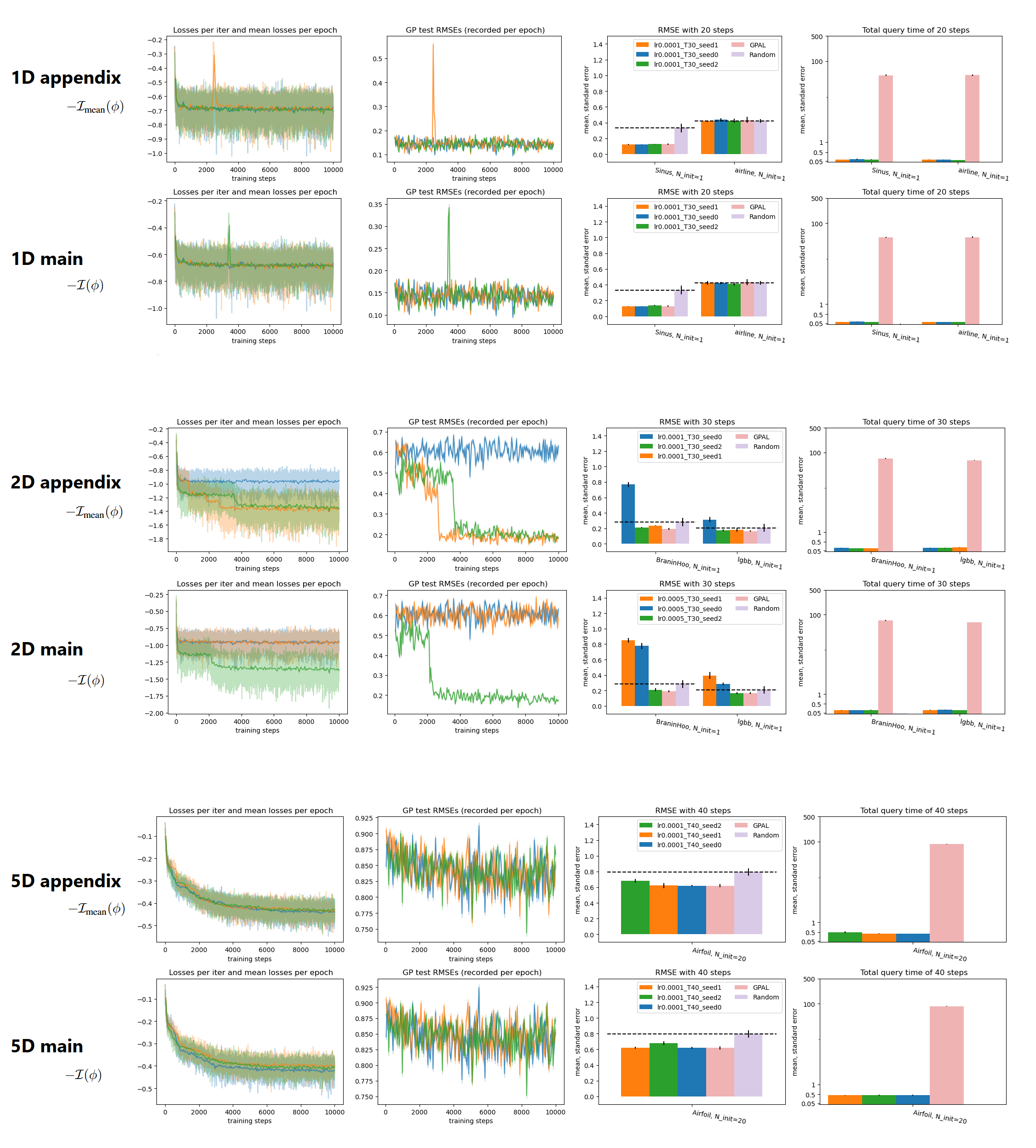
Figure A.G.8: Unconstrained AL results of objectives main $\mathcal{I}$ (Eq. 5) and appendix $\mathcal{I}_{\text{mean}}$ (Eq. A.15). The numerical congifurations (e.g. $D,T$) are identical for both objectives (Tables A.E.2, A.F.4 and A.E.3).We deploy the policy with $T=20$ for $1D$, $T=30$ for $2D$, and $T=40$ for $5D$ problems. The first column shows the training losses $-\mathcal{I}$ or $-\mathcal{I}_{\text{mean}}$ per training step and per epoch mean (mean of 50 steps). At the end of each epoch, we sample a batch of GP functions, not for training, but we deploy the policy for $T$ steps (e.g. train $T_{\text{sim}}\leq T=30$, then deploy $T=30$) and evaluate the GP RMSE against the ground truth. The GP RMSEs per training epoch are shown in the second column. After the training, we deploy each policy on benchmark problems and the results are the third and fourth columns (time illustrated in seconds).

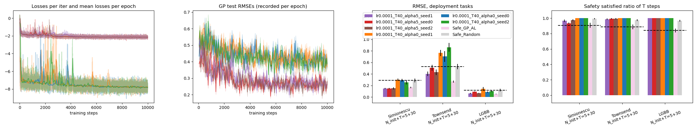
Figure A.G.9: The main safe AL objective $\mathcal{S}_{\mathcal{H}}$ with $\gamma=0.05$ vs $\gamma=0$, on $2D$ problems. The training loss values $-\mathcal{S}_{\mathcal{H}}$ are dominated by the minimized likelihood of unsafe queries if $\gamma=0$ (first column), and the AL exploration is deteriorated in the training, as indicated by the RMSEs against ground truth GPs (second column). After the training, the policies are deployed on three problems, and the results show similar exploration and safety trade-off as observed during the training (third and fourth columns). The deployment colored bars are sorted according to the averaged training losses of the last 10 epochs (left to right: highest to lowest losses). The baseline methods Safe GP AL and Safe Random are deployed with $\gamma=0.05$. When $\gamma=0$, a conventional safe AL cannot operates because the entire input space will be identified unsafe.

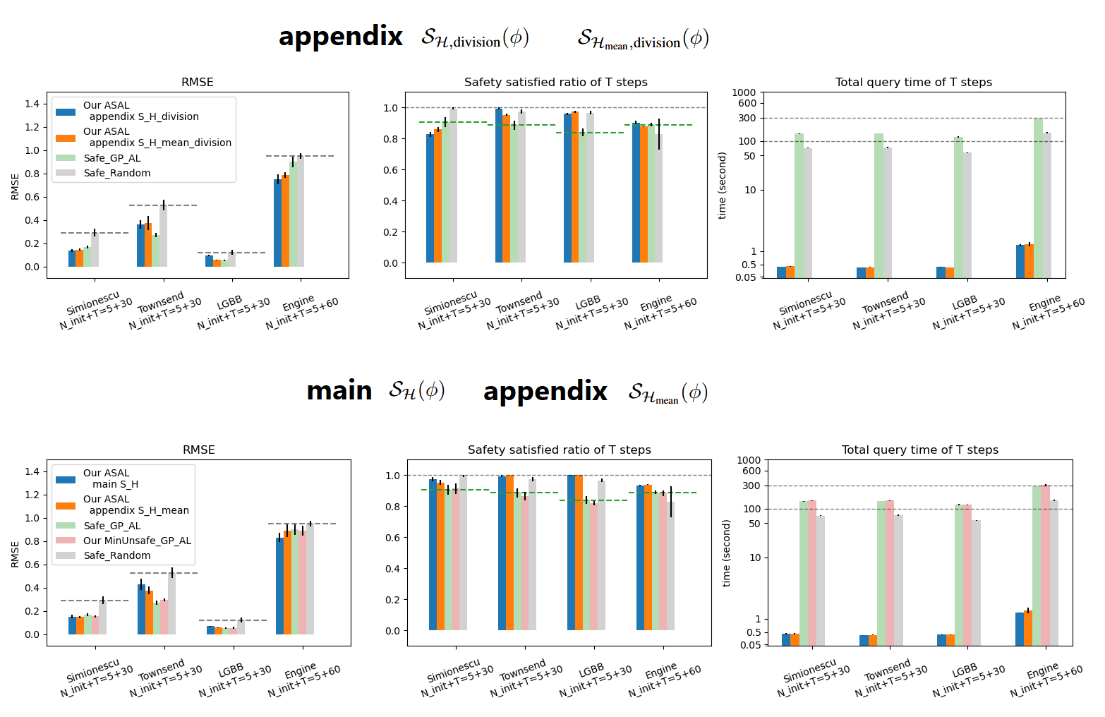
Figure A.G.10: Results of different amortized safe AL objectives and the safe AL of MinUnsafe criterion. Our safe AL policies are trained on four objectives: main $\mathcal{S}_{\mathcal{H}},\gamma=0.05$, appendix $\mathcal{S}_{\mathcal{H}_{\text{mean}}},\gamma=0.05$, and appendix $\mathcal{S}_{\mathcal{H},\text{division}},\mathcal{S}_{\mathcal{H}_{\text{mean}},\text{division}}$ which have no $\gamma$ clamping. As ordered in Figure A.C.6, $\mathcal{S}_{\mathcal{H},\text{division}},\mathcal{S}_{\mathcal{H}_{\text{mean}},\text{division}}$ are on the top and $\mathcal{S}_{\mathcal{H}},\mathcal{S}_{\mathcal{H}_{\text{mean}}}$ are at the bottom. The MinUnsafe acquisition function corresponds to $\mathcal{S}_{\mathcal{H}},\mathcal{S}_{\mathcal{H}_{\text{mean}}}$ objectives and is thus shown at the bottom.

G.1 Unconstrained AL Objectives, Main vs Appendix

This experiment provide two pieces of information: (i) how the training is monitored, and (ii) comparison of the main objective and appendix objective.

We compare the two objectives $\mathcal{I},\mathcal{I}_{\text{mean}}$ (Eqs. 5 and A.15) under the same numerical setup as described in Tables A.E.2 and A.F.4. These objectives have the same complexity (Table A.E.3).

At the end of each training epoch, we sample GP functions, deploy the policy for $T$ steps, where this $T$ is the training max sequence length, and then we use the ground truth GP and the $T$ queries to evaluate the modeling RMSE. We call this the GP test RMSE. Please be aware of the difference that we deploy policies on benchmarks problems after training, and such deployment RMSE requires GP fitting as ground truth is not available.

In Figure A.G.8, we demonstrate the training losses (negative training objectives) as well as the deployment results. The behavior of the two objectives do not seem to have obvious differences. Note that this paper use RBF kernels, which means the functions are assumed stationary. To avoid confusion, we perform only Type II maximum likelihood (no AGP) for the deployment GP modeling.

The training loss and GP test RMSE appear to be good indicators of the training performance, as the $1D$ and $2D$ examples show good deployments for policies of good training loss or GP test RMSE (Figure A.G.8). The $2D$ policies sometimes get stuck in patterns where queries are put only at the border of $\mathcal{X}$, namely those with worse training losses and GP test RMSEs. This pattern happens way more often if we train with the entropy losses $\mathcal{H},\mathcal{H}_{\text{mean}}$ (results not shown).

The policies shown in our main paper are the one here with the best average training loss in the last 10 epochs (last 500 training steps).

G.2 Main Safe AL Objective, $\gamma=0.05$ vs $\gamma=0$

We train on $2D$ with $\mathcal{S}_{\mathcal{H}},\gamma=0.05$ or $\gamma=0$ (Eq. 7). To avoid confusion, we perform only Type II maximum likelihood for GP modeling. We see from Figure A.G.9 that $\gamma=0$ makes the safety scores dominate the loss values. As a result, the deployment is safer but the collected data lead to worse modeling performance.

Please be aware that our policy still does not need GP to deploy, which means we are faster than all the GP-based baselines, including Safe Random. Overall, we should specify $\gamma$ depending on the safety criticality.

We train with a few different random seed values. In our main paper, we again select the policy based on the average loss values of the last 10 epochs (last 500 training steps).

G.3 Amortized Safe AL Objectives Main vs Appendix, Safe AL of Minimum Unsafe Criterion Eq. 6

We compare a couple of methods:

1. safe AL of policy trained on our main $\mathcal{S}_{\mathcal{H}}$, $\gamma=$5% (Eq. 7),

2. safe AL of policy trained on our appendix $\mathcal{S}_{\mathcal{H}_{\text{mean}}}$, $\gamma=$5% (unconstrained $\mathcal{H}_{\text{mean}}$ decorated with our main min unsafe likelihood, see Figure A.C.6),

3. safe AL of policy trained on our appendix $\mathcal{S}_{\mathcal{H},\text{division}}$ (unconstrained $\mathcal{H}$ decorated with our appendix max safe likelihood, see Eqs. A.17 and A.C.6),

4. safe AL of policy trained on our appendix $\mathcal{S}_{\mathcal{H}_{\text{mean}},\text{division}}$ (unconstrained $\mathcal{H}_{\text{mean}}$ decorated with our appendix max safe likelihood, see Figure A.C.6), and

5. conventional GP based safe AL (Algorithm A.9) but we add the unconstrained safety-aware acquisition criterion (Eq. 6), named MinUnsafe GP AL: $\bm{x}_{t}=\text{argmax}\{\mathbb{H}[y(\bm{x})|y_{1:t-1},Y_{\text{init}}]-\log\text{max}(\gamma,p(z(\bm{x})<0|z_{1:t-1},Z_{\text{init}}))\}$ ($\gamma=0.05$, this is the same as Eq. 6 if we take expectation over the forecasted $y(\bm{x})$, and this corresponds to objectives $\mathcal{S}_{\mathcal{H}},\mathcal{S}_{\mathcal{H}_{\text{mean}}}$, see the paragraph of Eqs. 6 and 7).

All objectives are leveraged under the same numerical setup as described in Tables A.E.2 and A.F.4. These objectives have the same complexity (Table A.E.3).

To avoid confusion, we perform only Type II maximum likelihood for GP modeling. We demonstrate the result on $2D$ problems (Figure A.G.10). Firstly, the performance of Safe GP AL (constrained predictive entropy acquisition) does not seem to have obvious empirical differences from MinUnsafe GP AL. This shows an advantage of MinUnsafe GP AL because its acquisition criterion is safety-aware but unconstrained, and an unconstrained optimization is much easier to be solved. Note that, for a fair comparison, our paper solves the acquisition optimization of MinUnsafe GP AL on discretized set.

Our ASAL policies trained with different objectives all seem to query reasonable data. In average, minimizing unsafe likelihood ($\mathcal{S}_{\mathcal{H}},\mathcal{S}_{\mathcal{H}_{\text{mean}}}$) prioritizes safety over AL exploration. This is consistent to what we observe from the objective values (Figure A.C.6).

References

- Altman (1999) Altman, E. Constrained markov decision processes. Routledge, 1999.
- Andersson et al. (2017) Andersson, O., Wzorek, M., and Doherty, P. Deep learning quadcopter control via risk-aware active learning. AAAI Conference on Artificial Intelligence, 2017.
- Berkenkamp et al. (2016) Berkenkamp, F., Schoellig, A. P., and Krause, A. Safe controller optimization for quadrotors with gaussian processes. International Conference on Robotics and Automation, 2016.
- Berkenkamp et al. (2020) Berkenkamp, F., Krause, A., and Schoellig, A. P. Bayesian optimization with safety constraints: Safe and automatic parameter tuning in robotics. Machine Learning, 2020.
- Bingham et al. (2018) Bingham, E., Chen, J. P., Jankowiak, M., Obermeyer, F., Pradhan, N., Karaletsos, T., Singh, R., Szerlip, P., Horsfall, P., and Goodman, N. D. Pyro: Deep Universal Probabilistic Programming. Journal of Machine Learning Research, 2018.
- Bitzer et al. (2023) Bitzer, M., Meister, M., and Zimmer, C. Amortized inference for gaussian process hyperparameters of structured kernels. Conference on Uncertainty in Artificial Intelligence, 2023.
- Bottero et al. (2022) Bottero, A., Luis, C., Vinogradska, J., Berkenkamp, F., and Peters, J. R. Information-theoretic safe exploration with gaussian processes. Advances in Neural Information Processing Systems, 2022.
- Brochu et al. (2010) Brochu, E., Cora, V. M., and de Freitas, N. A tutorial on bayesian optimization of expensive cost functions, with application to active user modeling and hierarchical reinforcement learning. arXiv, 2010.
- Brunke et al. (2022) Brunke, L., Greeff, M., Hall, A. W., Yuan, Z., Zhou, S., Panerati, J., and Schoellig, A. P. Safe learning in robotics: From learning-based control to safe reinforcement learning. Annual Review of Control, Robotics, and Autonomous Systems, 2022.
- Chen et al. (2017) Chen, Y., Hoffman, M. W., Colmenarejo, S. G., Denil, M., Lillicrap, T. P., Botvinick, M., and de Freitas, N. Learning to learn without gradient descent by gradient descent. International Conference on Machine Learning, 2017.
- Citovsky et al. (2021) Citovsky, G., DeSalvo, G., Gentile, C., Karydas, L., Rajagopalan, A., Rostamizadeh, A., and Kumar, S. Batch active learning at scale. Advances in Neural Information Processing Systems, 2021.
- Foster et al. (2021) Foster, A., Ivanova, D. R., Malik, I., and Rainforth, T. Deep Adaptive Design: Amortizing Sequential Bayesian Experimental Design. International Conference on Machine Learning, 2021.
- García et al. (2015) García, J., Fern, and o Fernández. A comprehensive survey on safe reinforcement learning. Journal of Machine Learning Research, 2015.
- Gelbart et al. (2014) Gelbart, M. A., Snoek, J., and Adams, R. P. Bayesian optimization with unknown constraints. Conference on Uncertainty in Artificial Intelligence, 2014.
- Gramacy et al. (2015) Gramacy, R. B., Gray, G. A., Digabel, S. L., Lee, H. K. H., Ranjan, P., Wells, G., and Wild, S. M. Modeling an augmented lagrangian for blackbox constrained optimization. arXiv, 2015.
- Griffiths & Hernández-Lobato (2020) Griffiths, R.-R. and Hernández-Lobato, J. M. Constrained Bayesian optimization for automatic chemical design using variational autoencoders. Chemical Science, 2020.
- Gu et al. (2024) Gu, S., Yang, L., Du, Y., Chen, G., Walter, F., Wang, J., and Knoll, A. A review of safe reinforcement learning: Methods, theories and applications. IEEE Transactions on Pattern Analysis and Machine Intelligence, 2024.
- Guestrin et al. (2005) Guestrin, C., Krause, A., and Singh, A. P. Near-optimal sensor placements in gaussian processes. International Conference on Machine Learning, 2005.
- Hensman et al. (2015) Hensman, J., Matthews, A., and Ghahramani, Z. Scalable Variational Gaussian Process Classification. International Conference on Artificial Intelligence and Statistics, 2015.
- Ivanova et al. (2021) Ivanova, D. R., Foster, A., Kleinegesse, S., Gutmann, M. U., and Rainforth, T. Implicit Deep Adaptive Design: Policy-Based Experimental Design without Likelihoods. Advances in Neural Information Processing Systems, 2021.
- Kirschner et al. (2019) Kirschner, J., Mutny, M., Hiller, N., Ischebeck, R., and Krause, A. Adaptive and safe Bayesian optimization in high dimensions via one-dimensional subspaces. International Conference on Machine Learning, 2019.
- Krause & Guestrin (2007) Krause, A. and Guestrin, C. Nonmyopic active learning of gaussian processes: An exploration-exploitation approach. International Conference on Machine Learning, 2007.
- Krause et al. (2008) Krause, A., Singh, A., and Guestrin, C. Near-optimal sensor placements in gaussian processes: Theory, efficient algorithms and empirical studies. Journal of Machine Learning Research, 2008.
- Kumar & Gupta (2020) Kumar, P. and Gupta, A. Active learning query strategies for classification, regression, and clustering: A survey. Journal of Computer Science and Technology, 2020.
- Lederer et al. (2021) Lederer, A., Conejo, A. J. O., Maier, K. A., Xiao, W., Umlauft, J., and Hirche, S. Gaussian process-based real-time learning for safety critical applications. International Conference on Machine Learning, 2021.
- Li et al. (2022) Li, C.-Y., Rakitsch, B., and Zimmer, C. Safe active learning for multi-output gaussian processes. International Conference on Artificial Intelligence and Statistics, 2022.
- Li et al. (2024) Li, C.-Y., Duennbier, O., Toussaint, M., Rakitsch, B., and Zimmer, C. Global safe sequential learning via efficient knowledge transfer. arXiv, 2024.
- Liu et al. (2020a) Liu, L., Jiang, H., He, P., Chen, W., Liu, X., Gao, J., and Han, J. On the variance of the adaptive learning rate and beyond. International Conference on Learning Representations, 2020a.
- Liu et al. (2020b) Liu, S., Sun, X., Ramadge, P. J., and Adams, R. P. Task-agnostic amortized inference of gaussian process hyperparameters. Advances in Neural Information Processing Systems, 2020b.
- Moss et al. (2023) Moss, H. B., Ober, S. W., and Picheny, V. Inducing point allocation for sparse gaussian processes in high-throughput bayesian optimisation. International Conference on Artificial Intelligence and Statistics, 2023.
- Nguyen–Tuong & Peters (2010) Nguyen–Tuong, D. and Peters, J. Incremental sparsification for real-time online model learning. International Conference on Artificial Intelligence and Statistics, 2010.
- Nocedal & Wright (2006) Nocedal, J. and Wright, S. J. Numerical optimization. Springer, 2006.
- Pamadi et al. (2004) Pamadi, B. N., Covell, P. F., Tartabini, P. V., and Murphy, K. J. Aerodynamic characteristics and glide-back performance of langley glide-back booster. Applied Aerodynamics Conference and Exhibit, 2004.
- Pescador-Barrios et al. (2024) Pescador-Barrios, G., Filippi, S., and van der Wilk, M. ”how big is big enough?” adjusting model size in continual gaussian processes. arXiv, 2024.
- Rahimi & Recht (2007) Rahimi, A. and Recht, B. Random features for large-scale kernel machines. Advances in Neural Information Processing Systems, 2007.
- Rainforth et al. (2024) Rainforth, T., Foster, A., Ivanova, D. R., and Smith, F. B. Modern Bayesian Experimental Design. Statistical Science, 2024.
- Rasmussen & Williams (2006) Rasmussen, C. and Williams, C. Gaussian processes for machine learning. MIT Press, 2006.
- Rogers et al. (2003) Rogers, S. E., Aftosmis, M. J., Pandya, S. A., Chaderjian, N. M., T., E. T., and Ahmad, J. U. Automated cfd parameter studies on distributed parallel computers. AIAA Computational Fluid Dynamics Conference, 2003.
- Rothfuss et al. (2021) Rothfuss, J., Fortuin, V., Josifoski, M., and Krause, A. Pacoh: Bayes-optimal meta-learning with pac-guarantees. International Conference on Machine Learning, 2021.
- Schreiter et al. (2015) Schreiter, J., Nguyen-Tuong, D., Eberts, M., Bischoff, B., Markert, H., and Toussaint, M. Safe exploration for active learning with gaussian processes. Machine Learning and Knowledge Discovery in Databases, 2015.
- Seeger (2004) Seeger, M. Low rank updates for the cholesky decomposition. 2004.
- Seo et al. (2000) Seo, S., Wallat, M., Graepel, T., and Obermayer, K. Gaussian process regression: active data selection and test point rejection. International Joint Conference on Neural Networks, 2000.
- Settles (2010) Settles, B. Active learning literature survey. University of Wisconsin-Madison, 2010.
- Simionescu (2014) Simionescu, P. Computer-aided graphing and simulation tools for autocad users. Computer-Aided Graphing and Simulation Tools for AutoCAD Users, 2014.
- Srinivas et al. (2012) Srinivas, N., Krause, A., Kakade, S. M., and Seeger, M. W. Information-theoretic regret bounds for gaussian process optimization in the bandit setting. IEEE Transactions on Information Theory, 2012.
- Sui et al. (2015) Sui, Y., Gotovos, A., Burdick, J., and Krause, A. Safe exploration for optimization with gaussian processes. International Conference on Machine Learning, 2015.
- Swersky et al. (2020) Swersky, K., Rubanova, Y., Dohan, D., and Murphy, K. Amortized bayesian optimization over discrete spaces. Conference on Uncertainty in Artificial Intelligence, 2020.
- Tharwat & Schenck (2023) Tharwat, A. and Schenck, W. A survey on active learning: State-of-the-art, practical challenges and research directions. Mathematics, 2023.
- Titsias (2009) Titsias, M. Variational learning of inducing variables in sparse gaussian processes. International Conference on Artificial Intelligence and Statistics, 2009.
- Townsend (2017) Townsend, A. Constrained optimization in chebfun. chebfun.org, 2017.
- Vaswani et al. (2017) Vaswani, A., Shazeer, N., Parmar, N., Uszkoreit, J., Jones, L., Gomez, A. N., Kaiser, L. u., and Polosukhin, I. Attention is all you need. Advances in Neural Information Processing Systems, 2017.
- Wang et al. (2019) Wang, K., Pleiss, G., Gardner, J., Tyree, S., Weinberger, K. Q., and Wilson, A. G. Exact gaussian processes on a million data points. Advances in Neural Information Processing Systems, 2019.
- Wilson et al. (2020) Wilson, J. T., Borovitskiy, V., Terenin, A., Mostowsky, P., and Deisenroth, M. P. Efficiently sampling functions from gaussian process posteriors. International Conference on Machine Learning, 2020.
- Yanan Sui et al. (2018) Yanan Sui, Vincent Zhuang, Joel W. Burdick, and Yisong Yue. Stagewise Safe Bayesian Optimization with Gaussian Processes. International Conference on Machine Learning, 80, 2018.
- Zimmer et al. (2018) Zimmer, C., Meister, M., and Nguyen-Tuong, D. Safe active learning for time-series modeling with gaussian processes. Advances in Neural Information Processing Systems, 2018.