Visual Generation Without Guidance

Abstract

Classifier-Free Guidance (CFG) has been a default technique in various visual generative models, yet it requires inference from both conditional and unconditional models during sampling. We propose to build visual models that are free from guided sampling. The resulting algorithm, Guidance-Free Training (GFT), matches the performance of CFG while reducing sampling to a single model, halving the computational cost. Unlike previous distillation-based approaches that rely on pretrained CFG networks, GFT enables training directly from scratch. GFT is simple to implement. It retains the same maximum likelihood objective as CFG and differs mainly in the parameterization of conditional models. Implementing GFT requires only minimal modifications to existing codebases, as most design choices and hyperparameters are directly inherited from CFG. Our extensive experiments across five distinct visual models demonstrate the effectiveness and versatility of GFT. Across domains of diffusion, autoregressive, and masked-prediction modeling, GFT consistently achieves comparable or even lower FID scores, with similar diversity-fidelity trade-offs compared with CFG baselines, all while being guidance-free. Code will be available at https://github.com/thu-ml/GFT.

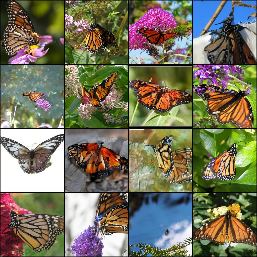
$\beta=1.0$

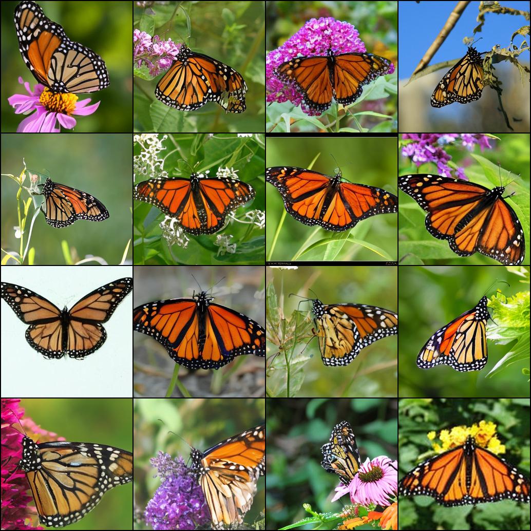
$\beta=0.5$

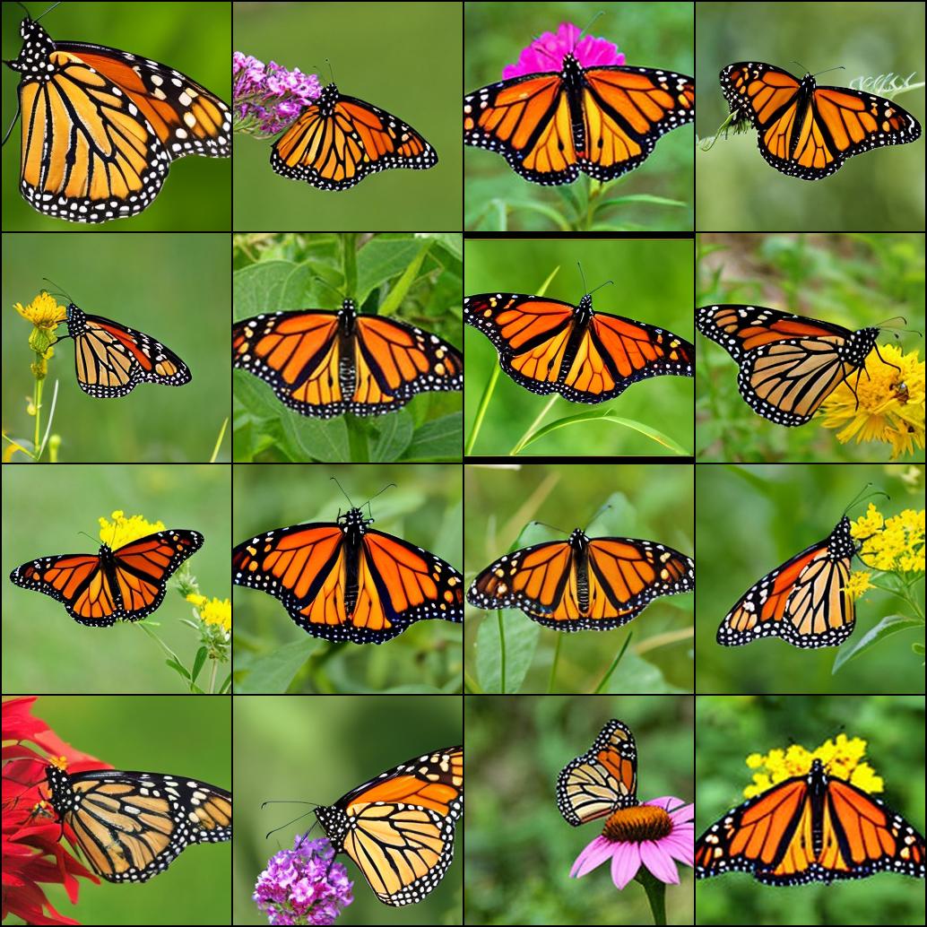
$\beta=0.25$

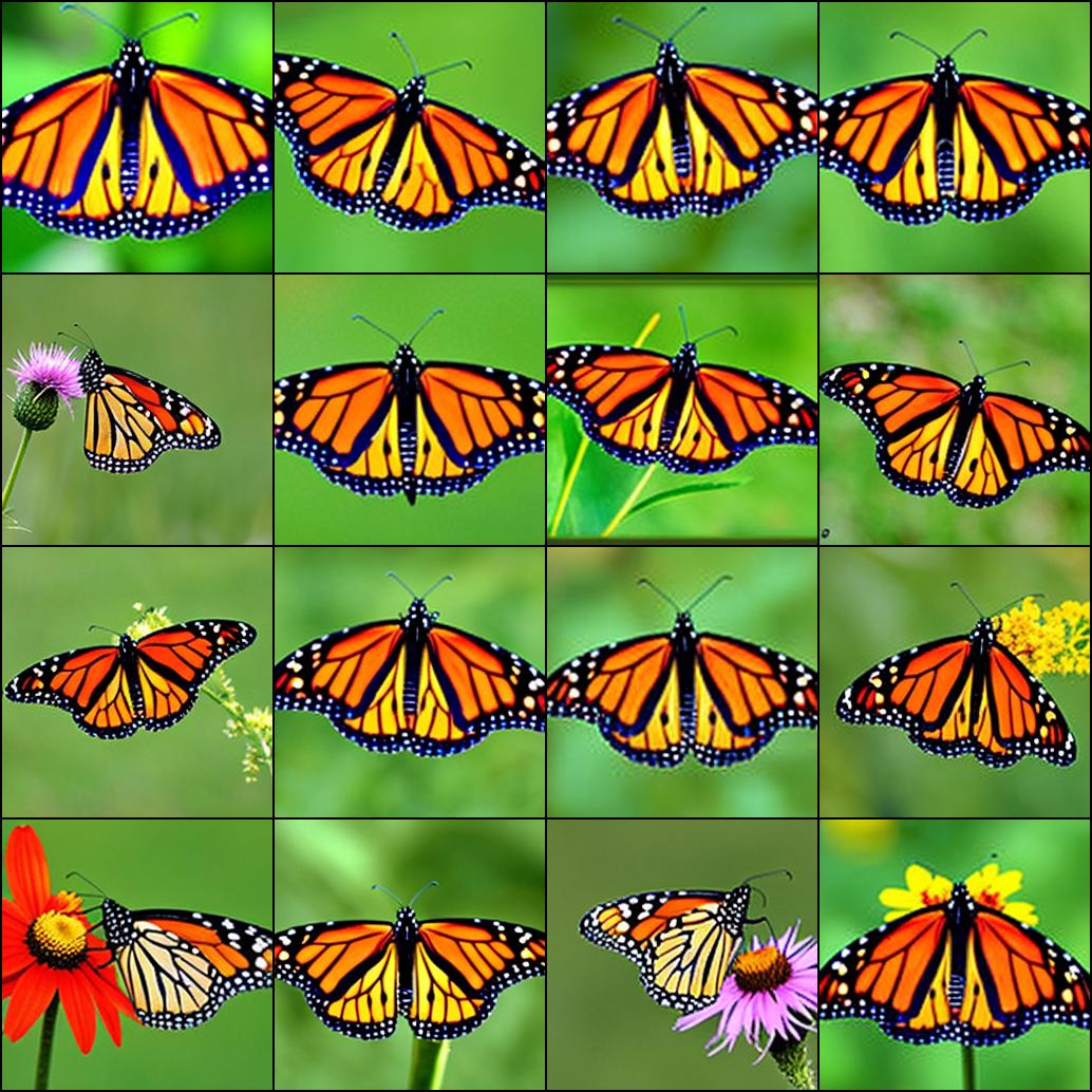
$\beta=0.1$

Figure 1: Impact of adjusting sampling temperature $\beta$ for DiT-XL/2 after applying GFT. More examples are in Figure 11.

1 Introduction

Low-temperature sampling is a critical technique for enhancing generation quality by focusing only on the model’s high-likelihood areas. Visual models mainly achieved this through Classifier-Free Guidance (CFG) (Ho & Salimans, 2022). CFG jointly optimizes both conditional and unconditional models during training and combines them to define the sampling process. By altering the guidance scale, it can flexibly trade off image fidelity and diversity at inference time, while significantly improving sample quality. Due to its effectiveness, CFG has been a default technique for a wide spectrum of visual generative models, including diffusion (Ho et al., 2020), autoregressive (AR) (Chen et al., 2020; Tian et al., 2024), and masked-prediction models (Chang et al., 2022; Li et al., 2023).

Despite the wide application, CFG requires inferencing both conditional and unconditional models to achieve the sampling distribution. This not only doubles the sampling cost but also complicates the post-training of visual models: When distilling pretrained diffusion models (Meng et al., 2023; Luo et al., 2023; Yin et al., 2024b) for fast inference or applying RLHF techniques (Black et al., 2023; Chen et al., 2024b), CFG requires the extra unconditional model to be additionally considered in the algorithm design.

It’s also worth noting that for language models (LMs), a single model is sufficient to represent sampling distributions across various temperatures. However, similarly following LMs’ approach to divide model output by a constant temperature value has largely been found ineffective in visual sampling (Dhariwal & Nichol, 2021), even for visual AR models with similar architecture to LMs (Sun et al., 2024). This leaves us wondering, how can we control the sampling temperature for visual models using only one model?

Existing attempts mainly include distillation methods for diffusion models (Meng et al., 2023; Luo et al., 2023; Yin et al., 2024b) and alignment methods for AR models (Chen et al., 2024b). These methods rely heavily on pretrained CFG networks for loss definition and do not support training guidance-free models from scratch. Their two-stage optimization pipeline may also lead to performance loss compared with CFG, even after extensive tuning. Generalizability is also a concern. Current methods are tailored for either continuous diffusion models or discrete AR models, lacking the versatility to cover all domains.

We propose Guidance-Free Training (GFT) as a foundational algorithm for building guidance-free visual generative models. GFT matches CFG in performance while requiring only a single model for temperature-controlled sampling (Figure 1), effectively halving sampling costs. It offers stable and efficient training with the same convergence rate as CFG, almost no extra memory usage, and only 10–20% additional computation per training update. Notably, GFT is highly versatile, applicable in all visual domains within CFG’s scope, including diffusion, AR, and masked models.

The core idea behind GFT is straightforward (Figure 2). GFT and CFG optimize the same conditional loss. CFG parameterizes an independent conditional model and combines it with another unconditional model for guided sampling. Contrastively, GFT does not explicitly define a conditional model. Instead, it constructs the conditional model as a linear interpolation between a sampling model and the unconditional model. By training this implicit network, GFT directly optimizes the underlying sampling model, which is then employed for visual generation without guidance. In essence, one can consider GFT simply as a conditional parameterization technique in CFG training. This perspective makes GFT extremely easy to implement based on existing codebases, requiring only a few lines of modifications and with most design choices and hyperparameters inherited.

We verify the effectiveness and efficiency of GFT in both class-to-image and text-to-image tasks, spanning 5 distinctive types of visual models: DiT (Peebles & Xie, 2023), VAR (Tian et al., 2024), LlamaGen (Sun et al., 2024), MAR (Li et al., 2024) and LDM (Rombach et al., 2022). Across all models, GFT enjoys almost lossless FID in fine-tuning existing CFG models into guidance-free models (Sec. 5.2). For instance, we achieve a guidance-free FID of 1.99 for the DiT-XL model with only 2% of pretraining epochs, while the CFG performance is 2.11. This surpasses previous distillation and alignment methods in their respective application domains. GFT also demonstrates great superiority in building guidance-free models from scratch. With the same amount of training epochs, GFT models generally match or even outperform CFG models, despite being $50\%$ cheaper in sampling (Sec. 5.3). By taking in a temperature parameter as model input, GFT can achieve a flexible diversity-fidelity trade-off similar to CFG (Sec. 5.4).

Our main contribution is GFT as a fundamental visual generative modeling objective. GFT enables effective low-temperature visual generation without guided sampling. We hope it leads to a new paradigm of visual generative training.

2 Background

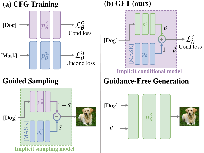
Figure 2: Comparison of GFT and CFG method. GFT shares CFG’s training objective but has a different parameterization technique for the conditional model. This enables direct training of an explicit sampling model.

2.1 Visual Generative Modeling

Continuous diffusion models.

Diffusion models (Ho et al., 2020) define a forward process that gradually injects noises into clean images from data distribution $p({\bm{x}})$:

$${\bm{x}}_{t}=\alpha_{t}{\bm{x}}+\sigma_{t}\bm{\epsilon},$$

where $t\in[0,1]$, and $\bm{\epsilon}$ is standard Gaussian noise. $\alpha_{t},\sigma_{t}$ defines the denoising schedule. We have

$$p_{t}({\bm{x}}_{t})=\int{\mathcal{N}}({\bm{x}}_{t}|\alpha_{t}{\bm{x}},\sigma_{t}^{2}{\bm{I}})p({\bm{x}})\mathrm{d}{\bm{x}},$$

where $p_{0}({\bm{x}})=p({\bm{x}})$ and $p_{1}\approx{\mathcal{N}}(0,1)$.

Given dataset $p({\bm{x}},{\bm{c}})$, we can train conditional diffusion models by predicting the Gaussian noise added to ${\bm{x}}_{t}$.

$$\min_{\theta}\mathbb{E}_{p({\bm{x}},{\bm{c}}),t,\bm{\epsilon}}\left[\|\epsilon_{\theta}({\bm{x}}_{t}|{\bm{c}})-\bm{\epsilon}\|_{2}^{2}\right].$$ (1)

More formally, Song et al. (2021) proved that Eq. 1 is essentially performing maximum likelihood training with evidence lower bound (ELBO). Also, the denoising model $\epsilon_{\theta}^{*}$ eventually converges to the data score function:

$$\epsilon_{\theta}^{*}({\bm{x}}_{t}|{\bm{c}})=-\sigma_{t}\nabla_{{\bm{x}}_{t}}\log p_{t}({\bm{x}}_{t}|{\bm{c}})$$ (2)

Given condition ${\bm{c}}$, $\epsilon_{\theta}$ can be leveraged to generate images from $p_{\theta}({\bm{x}}|{\bm{c}})$ by denoising noises from $p_{1}$ iteratively.

Discrete AR & masked models.

AR models (Chen et al., 2020) and masked-prediction models (Chang et al., 2022) function similarly. Both discretize images ${\bm{x}}$ into token sequences ${\bm{x}}_{1:N}$ and then perform token prediction. Their maximum likelihood training objective can be unified as

$$\min_{\theta}\mathbb{E}_{p({\bm{x}}_{1:N},{\bm{c}})}-\sum_{i}p_{\theta}({\bm{x}}_{n}|{\bm{x}}_{<n},{\bm{c}}).$$ (3)

For AR models, ${\bm{x}}_{<n}$ represents the first $i$ tokens in a pre-determined order, and ${\bm{x}}_{i}$ is the next token to be predicted. For masked models, ${\bm{x}}_{i}$ represents all the unknown tokens that are randomized masked during training, while ${\bm{x}}_{<n}$ are the unmasked ones. Due to discrete modeling, the data likelihood $p_{\theta}$ in Eq. 3 can be easily calculated.

2.2 Classifier-Free Guidance

In diffusion modeling, vanilla temperature sampling (dividing model output by a constant value) is generally found ineffective in improving generation quality (Dhariwal & Nichol, 2021). Current methods typically employ CFG (Ho & Salimans, 2022), which redefines the sampling denoising function $\epsilon_{\theta}^{\text{s}}({\bm{x}}_{t}|c)$ using two denoising models:

$$\epsilon_{\theta}^{\text{s}}({\bm{x}}_{t}|c):=\epsilon_{\theta}^{\text{c}}({\bm{x}}_{t}|c)+s[\epsilon_{\theta}^{\text{c}}({\bm{x}}_{t}|c)-\epsilon_{\theta}^{\text{u}}({\bm{x}}_{t})],$$ (4)

where $\epsilon_{\theta}^{c}$ and $\epsilon_{\theta}^{\text{u}}$ respectively model the conditional data distribution $p(x|c)$ and the unconditional data distribution $p(x)$. In practice, $\epsilon_{\theta}^{\text{u}}$ can be jointly trained with $\epsilon_{\theta}^{c}$, by randomly masking the conditioning data in Eq. 1 with some fixed probability.

According to Eq. 2, CFG’s sampling distribution $p^{\text{s}}({\bm{x}}|c)$ has shifted from standard conditional distribution $p({\bm{x}}|{\bm{c}})$ to

$$p^{\text{s}}({\bm{x}}|c)\propto p({\bm{x}}|{\bm{c}})\left[\frac{p({\bm{x}}|{\bm{c}})}{p({\bm{x}})}\right]^{s}.$$ (5)

CFG offers an effective approach for lowering sampling temperature in visual generation by simply increasing $s>0$, thereby substantially improving sample quality.

Besides diffusion, CFG is also a critical sampling technique in discrete visual modeling (Chang et al., 2022; Team, 2024; Tian et al., 2024; Xie et al., 2024).

3 Method

Despite its effectiveness, CFG requires inferencing an extra unconditional model to guide the sampling process, directly doubling the computation cost.

Moreover, CFG complicates the post-training of visual generative models because the unconditional model needs to be additionally considered in algorithm design (Meng et al., 2023; Black et al., 2023).

We propose Guidance-Free Training (GFT) as an alternative method of CFG for improving sample quality in visual generation without guided sampling. GFT matches CFG in performance but only leverages a single model $\epsilon_{\theta}^{\text{s}}({\bm{x}}|c,s)$ to represent CFG’s sampling distribution $p^{\text{s}}({\bm{x}}|c)$.

We derive GFT’s training objective for diffusion models in Sec. 3.1, discuss its practical implementation in Sec. 3.2, and explain how it can be extended to discrete AR and masked models in Sec. 3.3.

3.1 Algorithm Derivation

The key challenge in directly learning sampling model $\epsilon_{\theta}^{s}$ is the absence of a dataset that aligns with distribution $p^{\text{s}}({\bm{x}}|c)$ in Eq. 5. It is impractical to optimize maximum-likelihood-training objectives like

$$\min_{\theta}\mathbb{E}_{\color[rgb]{1,0,0}{p^{s}({\bm{x}},{\bm{c}})}\color[rgb]{0,0,0},t,\bm{\epsilon}}\left[\|\epsilon_{\theta}^{s}({\bm{x}}_{t}|{\bm{c}})-\bm{\epsilon}\|_{2}^{2}\right].$$

because we cannot draw samples from $p^{\text{s}}$.

In contrast, training $\epsilon_{\theta}^{c}({\bm{x}}|{\bm{c}})$ and $\epsilon_{\theta}^{u}({\bm{x}})$ separately as in CFG is feasible because their corresponding datasets, $\{({\bm{x}},{\bm{c}})\sim p({\bm{x}},{\bm{c}})\}$ and $\{{\bm{x}}\sim p({\bm{x}})\}$, can be easily obtained.

To address this, we reformulate Eq. 4 by simple algebra:

$$\underbrace{\epsilon_{\theta}^{\text{c}}({\bm{x}}_{t}|c)}_{\begin{subarray}{c}\;\color[rgb]{0,0,1}p({\bm{x}}|{\bm{c}})\\ \text{Learnable}\end{subarray}}\;=\;\frac{1}{1+s}\underbrace{\epsilon_{\theta}^{\text{s}}({\bm{x}}_{t}|c)}_{\begin{subarray}{c}\color[rgb]{1,0,0}p^{s}({\bm{x}}|{\bm{c}})\\ \text{{\hskip-28.45274pt$\leftarrow$ \hskip 14.22636pt Target sampling model\hskip 14.22636pt +\hskip-28.45274pt}}\end{subarray}}\;+\;\frac{s}{1+s}\underbrace{\epsilon_{\theta}^{\text{u}}({\bm{x}}_{t})}_{\begin{subarray}{c}p({\bm{x}})\\ \text{Learnable}\end{subarray}}.$$ (6)

Although learning $\epsilon_{\theta}^{\text{s}}$ directly is difficult, we note it can be combined with an unconditional model $\epsilon_{\theta}^{\text{u}}$ to represent the standard conditional $\epsilon_{\theta}^{\text{c}}$, which is learnable. Thus, we can leverage the same conditional loss in Eq. 1 to train $\epsilon_{\theta}^{\text{s}}$:

$$\min_{\theta}\mathbb{E}_{\color[rgb]{0,0,1}p({\bm{x}},{\bm{c}})\color[rgb]{0,0,0},t,\bm{\epsilon}}\left[\|\frac{1}{1+s}\epsilon_{\theta}^{s}({\bm{x}}_{t}|{\bm{c}})+\frac{s}{1+s}\epsilon_{\theta}^{u}({\bm{x}}_{t})-\bm{\epsilon}\|_{2}^{2}\right],$$ (7)

where $\bm{\epsilon}$ is standard Gaussian noise, ${\bm{x}}_{t}=\alpha_{t}{\bm{x}}+\sigma_{t}\bm{\epsilon}$ are diffused images. $\alpha_{t}$ and $\sigma_{t}$ define the forward process.

To this end, we have a practical algorithm for directly learning guidance-free models $\epsilon_{\theta}^{s}$. However, unlike CFG which allows controlling sampling temperature by adjusting guidance scale $s$ to trade off fidelity and diversity, our method still lacks similar inference-time flexibility as Eq. 7 is performed for a specific $s$.

To solve this problem, we define a pseudo-temperature $\beta:=1/(1+s)$ and further condition our sampling model $\epsilon_{\theta}^{s}({\bm{x}}_{t}|{\bm{c}},\beta)$ on the extra $\beta$ input. We can randomly sample $\beta\in[0,1]$ during training, corresponding to $s\in[0,+\infty)$. The GFT objective in Eq. 7 now becomes:

$$\min_{\theta}\mathbb{E}_{p({\bm{x}},{\bm{c}}),t,\bm{\epsilon},\beta}\left[\|\beta\epsilon_{\theta}^{s}({\bm{x}}_{t}|{\bm{c}},\beta)+(1-\beta)\epsilon_{\theta}^{u}({\bm{x}}_{t})-\bm{\epsilon}\|_{2}^{2}\right].$$ (8)

When $\beta=1$, Eq. 8 reduces to conditional diffusion loss $\|\epsilon_{\theta}^{s}({\bm{x}}_{t}|{\bm{c}},\beta)-\bm{\epsilon}\|_{2}^{2}$. When $\beta=0$, Eq. 8 becomes an unconditional loss $\|\epsilon_{\theta}^{u}({\bm{x}}_{t})-\bm{\epsilon}\|_{2}^{2}$. This allows simultaneous training of both conditional and unconditional models.

As pseudo-temperature $\beta$ decreases $1\to 0$, the modeling target for $\epsilon_{\theta}^{s}$ gradually shifts from conditional data distribution $p({\bm{x}}|{\bm{c}})$ to lower-temperature distribution $p^{s}({\bm{x}}|{\bm{c}})$ as defined by Eq. 5.

3.2 Practical Implementation

Algorithm 1 Guidance-Free Training (Diffusion)

1: Initialize $\theta$ from pretrained models or from scratch.

2: for each gradient step do

3:   // CFG training w/ pseudo-temperature $\beta$

4:  ${\bm{x}},{\bm{c}}\sim p({\bm{x}},{\bm{c}})$

5:  $\beta\sim U(0,1)$, $t\sim U(0,1)$

6:  $\bm{\epsilon}\sim{\mathcal{N}}(\mathbf{0},{\bm{I}}^{2})$

7:  ${\bm{x}}_{t}=\alpha_{t}{\bm{x}}+\sigma_{t}\bm{\epsilon}$

8:  ${\bm{c}}_{\varnothing}={\bm{c}}$ masked by $\varnothing$ with $10\%$ probability

9:  Calculate $\epsilon_{\theta}^{s}({\bm{x}}_{t}|{\bm{c}}_{\varnothing},\beta)$ in training mode

10:   // Additional to CFG

11:   Calculate $\epsilon_{\theta}^{u}({\bm{x}}_{t}|\varnothing,1)$ in evaluation mode

12:  $\bm{\epsilon}_{\theta}=\beta\epsilon_{\theta}^{s}({\bm{x}}_{t}|{\bm{c}}_{\varnothing},\beta)+(1-\beta)\mathrm{\mathbf{sg}}[\epsilon_{\theta}^{u}({\bm{x}}_{t}|\varnothing,1)]$

13:   // Standard Maximum Likelihood Training

14:  $\theta\leftarrow\theta-\lambda\nabla_{\theta}\|\bm{\epsilon}_{\theta}-\bm{\epsilon}\|_{2}^{2}$    (Eq. 3.2)

15: end for

Eq. 3.2 presents a practical loss function of GFT. The implementation is in Algorithm 1.

$${\mathcal{L}}_{\theta}^{\text{diff}}({\bm{x}},{\bm{c}}_{\varnothing},t,\bm{\epsilon},\beta)$$

$$=\|\beta\epsilon_{\theta}^{s}({\bm{x}}_{t}|{\bm{c}}_{\varnothing},\beta)+(1-\beta)\mathrm{\mathbf{sg}}[\epsilon_{\theta}^{u}({\bm{x}}_{t}|\varnothing,1)]-\bm{\epsilon}\|_{2}^{2}.$$ (9)

Stopping the unconditional gradient.

The main difference between Eq. 3.2 and Eq. 8 is that $\epsilon_{\theta}^{u}$ is computed in evaluation mode, with model gradients stopped by the $\mathrm{\mathbf{sg}}[\cdot]$ operation. To train the model unconditionally, we randomly mask conditions ${\bm{c}}$ with $\varnothing$ when computing $\epsilon_{\theta}^{s}$. We show this design does not affect the training convergence point:

Theorem 1 (GFT Optimal Solution).

Given unlimited model capacity and training data, the optimal $\epsilon_{\theta^{*}}^{s}$ for optimizing Eq. 3.2 and Eq. 8 are the same. Both satisfy

$$\epsilon_{\theta^{*}}^{s}({\bm{x}}_{t}|{\bm{c}},\beta)$$

$$=-\sigma_{t}\left[\frac{1}{\beta}\nabla_{{\bm{x}}_{t}}\log p_{t}({\bm{x}}_{t}|{\bm{c}})-(\frac{1}{\beta}-1)\nabla_{{\bm{x}}_{t}}\log p_{t}({\bm{x}}_{t})\right]$$

Proof.

In Appendix B. ∎

The stopping-gradient technique has the following benefits:

(1) Alignment with CFG. The practical GFT algorithm (Eq. 3.2) differs from CFG training by a single unconditional inference step. This allows us to implement GFT with only a few lines of code based on existing codebases.

(2) Computational efficiency. Since the extra unconditional calculation is gradient-free. GFT requires virtually no extra GPU memory and only 19% additional train time per update vs. CFG (Figure 3). This stands in contrast with the naive implementation without gradient stopping (Eq. 8), which is equivalent to doubling the batch size for CFG training.

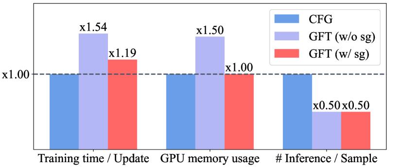
Figure 3: Comparison of computational efficiency between GFT and CFG. Estimated based on the DiT-XL model.

(3) Training stability. We empirically observe that stopping the gradient for the unconditional model could lead to better training stability and thus improved performance.

Table 1: Comparison of GFT (ours) and other guidance-free methods. Numbers are reported based on experiments for the DiT-XL model or the VAR-d30 model. We use 8$\times$80GB H100 GPU cards.

Method	Guidance Distillation	Condition Contrastive Alignment	Guidance-Free Training
Modeling target	$p_{\phi}^{c}+p_{\phi}^{u}\to p^{s}_{\theta}({\bm{x}}|{\bm{c}})$	$p_{\theta}^{s}+p_{\phi}^{c}\to\frac{p({\bm{x}}|{\bm{c}})}{p({\bm{x}})}$	$p_{\theta}^{s}+p_{\theta}^{u}\to p({\bm{x}}|{\bm{c}})$
Applicable area	Diffusion	AR & Masked	All
Loss form	$\left\|\bm{\epsilon}_{\theta}^{s}-[(1\!+\!s)\bm{\epsilon}_{\phi}^{c}-s\bm{\epsilon}_{\phi}^{u}]\right\|_{2}^{2}$	$-\!\log\!\sigma(r_{\theta}^{p})\!-\!\log\!\sigma(-r_{\theta}^{n});$ $r_{\theta}\!=\!\frac{1}{s}\log\frac{p_{\theta}^{s}}{p_{\phi}^{c}}$	$\beta f_{\theta}^{s}\!+\!(1\!\!-\!\!\beta)f_{\theta}^{u}$ + Diff/AR Loss
Train from scratch?	Not allowed	Not allowed	Allowed
# Inference / Update	3	4	2
Train time / Update	$\times$1.19	$\times$1.69	$\times$1.00
GPU memory usage	$\times$1.15	$\times$1.39	$\times$1.00

Input of $\beta$.

GFT requires an extra pseudo-temperature input in comparison with CFG. For this, we first process $\beta$ using the similar Fourier embedding method for diffusion time $t$ (Dhariwal & Nichol, 2021; Meng et al., 2023). This is followed by some MLP layers. Finally, the temperature embedding is added to the model’s original time or class embedding. If fine-tuning, we apply zero initialization for the final MLP layer so that $\beta$ would not affect model output at the start of training.

Hyperparameters.

Due to the high similarity between CFG and GFT training, we inherit most hyperparameter choices used for existing CFG models and mainly adjust parameters like learning rate during finetuning. When training from scratch, we find simply keeping all parameters the same with CFG is enough to yield good performance.

Training epochs.

When fine-tuning pretrained CFG models, we find 1% - 5% of pretraining epochs are sufficient to achieve nearly lossless FID performance. When from scratch, we always use the same training epochs compared with the CFG baseline.

3.3 GFT for AR and Masked Models

CFG is also a standard decoding method for discrete AR or masked visual models, critical to improving their sample quality (Chang et al., 2022; Li et al., 2023; Tian et al., 2024). Different from diffusion models which apply CFG in the score field, AR and masked models perform guided sampling on model logits:

$$\ell_{\theta}^{\text{s}}({\bm{x}}_{n}|{\bm{x}}_{<n},{\bm{c}})=$$

$$\ell_{\theta}^{\text{c}}({\bm{x}}_{n}|{\bm{x}}_{<n},{\bm{c}})+s[\ell_{\theta}^{\text{c}}({\bm{x}}_{n}|{\bm{x}}_{<n},{\bm{c}})-\ell_{\theta}^{\text{u}}({\bm{x}}_{n}|{\bm{x}}_{<n})].$$

Here ${\bm{x}}_{n}$ represents the $i$-th token of a tokenized image ${\bm{x}}$. $\ell_{\theta}$ are unnormalized model logits.

Similar to Sec. 3.1, we can derive the GFT objective for AR and masked models as standard cross-entropy loss:

$${\mathcal{L}}_{\theta}^{\text{AR}}({\bm{x}},{\bm{c}}_{\varnothing},\beta) =-\sum_{i}\log p_{\theta}^{s}({\bm{x}}_{n}|{\bm{x}}_{<n},{\bm{c}}_{\varnothing},\beta)$$ (10)

$$=-\sum_{i}\log\frac{e^{\ell_{\theta}^{s}({\bm{x}}_{n}|{\bm{x}}_{<n},{\bm{c}}_{\varnothing},\beta)}}{\sum_{w\in\mathcal{V}}e^{\ell_{\theta}^{s}(w|{\bm{x}}_{<n},{\bm{c}}_{\varnothing},\beta)}},$$ (11)

where $w$ is a token in the vocabulary $\mathcal{V}$, and

$$\ell_{\theta}^{s}(w|{\bm{x}}_{<n},{\bm{c}}_{\varnothing},\beta)$$

$$:=\beta\ell_{\theta}^{s}(w|{\bm{x}}_{<n},{\bm{c}}_{\varnothing},\beta)+(1-\beta)\mathrm{\mathbf{sg}}[\ell_{\theta}^{u}(w|{\bm{x}}_{<n})].$$ (12)

In Sec. 5, we apply GFT to a wide spectrum of visual generative models, including diffusion, AR, and masked models, demonstrating its versatility.

4 Connection with Other Guidance-Free Methods

Previous attempts to remove guided sampling from visual generation mainly include distillation methods for diffusion models and alignment methods for AR models. Alongside GFT, these methods all transform the sampling distribution $p^{s}$ into simpler, learnable forms, differing mainly in how they decompose the sampling distribution and set up modeling targets (Table 1).

Guidance Distillation (Meng et al., 2023) is quite straightforward, it simply learns a single model to match the output of pretrained CFG targets using L2 loss:

$${\mathcal{L}}_{\theta}^{\text{GD}}=\left\|\bm{\epsilon}_{\theta}^{s}({\bm{x}}_{t}|{\bm{c}},s)-\left[(1\!+\!s)\bm{\epsilon}_{\phi}^{c}({\bm{x}}_{t}|{\bm{c}})\!-\!s\bm{\epsilon}_{\phi}^{u}({\bm{x}}_{t})\right]\right\|_{2}^{2},$$ (13)

where $\bm{\epsilon}_{\phi}^{u}$ and $\bm{\epsilon}_{\phi}^{c}$ are pretrained models. ${\mathcal{L}}_{\theta}^{\text{GD}}$ breaks down the sampling model into a linear combination of conditional and unconditional models, which can be separately learned.

Despite being effective, Guidance distillation relies on pretrained CFG models as teacher models, and cannot be leveraged for from-scratch training. This results in an indirect, two-stage pipeline for learning guidance-free models. In comparison, our method unifies guidance-free training in one singular loss, allowing learning in an end-to-end style. Besides, GFT no longer requires learning an explicit conditional model $\bm{\epsilon}^{c}_{\theta}$. This saves training computation and VRAM usage. A detailed comparison is in Table 1.

Table 2: Model comparisons on the class-conditional ImageNet $256\times 256$ benchmark.

Model Type	FID $\downarrow$
	w/o Guidance	w/ Guidance
Diffusion Models
ADM  (Dhariwal & Nichol, 2021)	7.49	3.94
LDM-4  (Rombach et al., 2022)	10.56	3.60
U-ViT-H/2  (Bao et al., 2023)	–	2.29
MDTv2-XL/2  (Gao et al., 2023)	5.06	1.58
DiT-XL/2  (Peebles & Xie, 2023)	9.34	2.11
$\quad+$Distillation  (Meng et al., 2023)	2.11	–
$\quad+$GFT (Ours)	1.99	–
Autoregressive Models
VQGAN  (Esser et al., 2021)	15.78	5.20
ViT-VQGAN  (Yu et al., 2021)	4.17	3.04
RQ-Transformer  (Lee et al., 2022)	7.55	3.80
LlamaGen-3B  (Sun et al., 2024)	9.44	2.22
$\quad+$CCA  (Chen et al., 2024b)	2.69	–
$\quad+$GFT (Ours)	2.21	–
VAR-d30  (Tian et al., 2024)	5.26	1.92
$\quad+$CCA  (Chen et al., 2024b)	2.54	–
$\quad+$GFT (Ours)	1.91	–
Masked Models
MaskGIT  (Chang et al., 2022)	6.18	–
MAGVIT-v2  (Yu et al., 2023b)	3.65	1.78
MAGE  (Li et al., 2023)	6.93	–
MAR-B  (Li et al., 2024)	4.17	2.27
$\quad+$GFT (Ours)	2.39	–

Condition Contrastive Alignment (Chen et al., 2024b) constructs a preference pair for each image ${\bm{x}}$ in the dataset and applies similar preference alignment techniques for language models (Rafailov et al., 2023; Chen et al., 2024a) to fine-tune visual AR models:

$${\mathcal{L}}_{\theta}^{\text{CCA}}=-\!\log\!\sigma\left[r_{\theta}({\bm{x}},{\bm{c}}^{p})\right]\!-\!\log\!\sigma\left[-r_{\theta}({\bm{x}},{\bm{c}}^{n})\right],$$ (14)

where ${\bm{c}}^{p}$ is the preferred positive condition corresponding to the image ${\bm{x}}$, ${\bm{c}}^{n}$ is a negative condition randomly and independently sampled from the dataset. Given a conditional reference model $p_{\phi}^{c}$, the implicit reward $r_{\theta}$ is defined as

$$r_{\theta}({\bm{x}},{\bm{c}}):=\!\frac{1}{s}\log\frac{p_{\theta}^{s}({\bm{x}}|{\bm{c}})}{p_{\phi}^{c}({\bm{x}}|{\bm{c}})}.$$

CCA proves the optimal solution for solving Eq. 14 is $r_{\theta}^{*}=\log\frac{p({\bm{x}}|{\bm{c}})}{p({\bm{x}})}$, thus the convergence point for $p_{\theta}^{s}({\bm{x}}|{\bm{c}})$ also satisfies Eq. 5.

Both CCA and GFT train sampling model $p^{s}_{\theta}$ directly by combining it with another model to represent a learnable distribution. GFT leverages $\beta p^{s}_{\theta}+(1-\beta)p^{u}_{\theta}$ to represent standard conditional distribution $p({\bm{x}}|{\bm{c}})$, while CCA combines $p^{s}_{\theta}$ and pretrained $p_{\phi}({\bm{x}}|{\bm{c}})$ to represent the conditional residual $\log\frac{p({\bm{x}}|{\bm{c}})}{p({\bm{x}})}$. They also differ in applicable areas. CCA is based on language alignment losses, which requires calculating model likelihood $\log p_{\theta}$ during training. This forbids its direct application to diffusion models, where calculating exact likelihood is infeasible.

Table 3: Zero-shot text-to-image generation performance comparison on COCO 2014 validation set.

Text to Image Models	FID $\downarrow$
	w/o Guidance	w/ Guidance
GLIDE  (Nichol et al., 2021)	–	12.24
LDM  (Rombach et al., 2022)	–	12.63
DALL$\cdot$E 2  (Ramesh et al., 2022)	–	10.39
Stable Diffusion 1.5  (Rombach et al., 2022)	22.55	8.30
$\quad+$GFT (Ours)	8.32	–

5 Experiments

Our experiments aim to investigate:

1. GFT’s effectiveness and efficiency in fine-tuning CFG models into guidance-free variants (Sec. 5.2)

2. GFT’s ability in training guidance-free models from scratch, compared with classic CFG training (Sec. 5.3)

3. GFT’s capacity in controlling diversity-fidelity trade-off through temperature parameter $\beta$. (Sec. 5.4)

w/o Guidance

GFT (w/o Guidance)

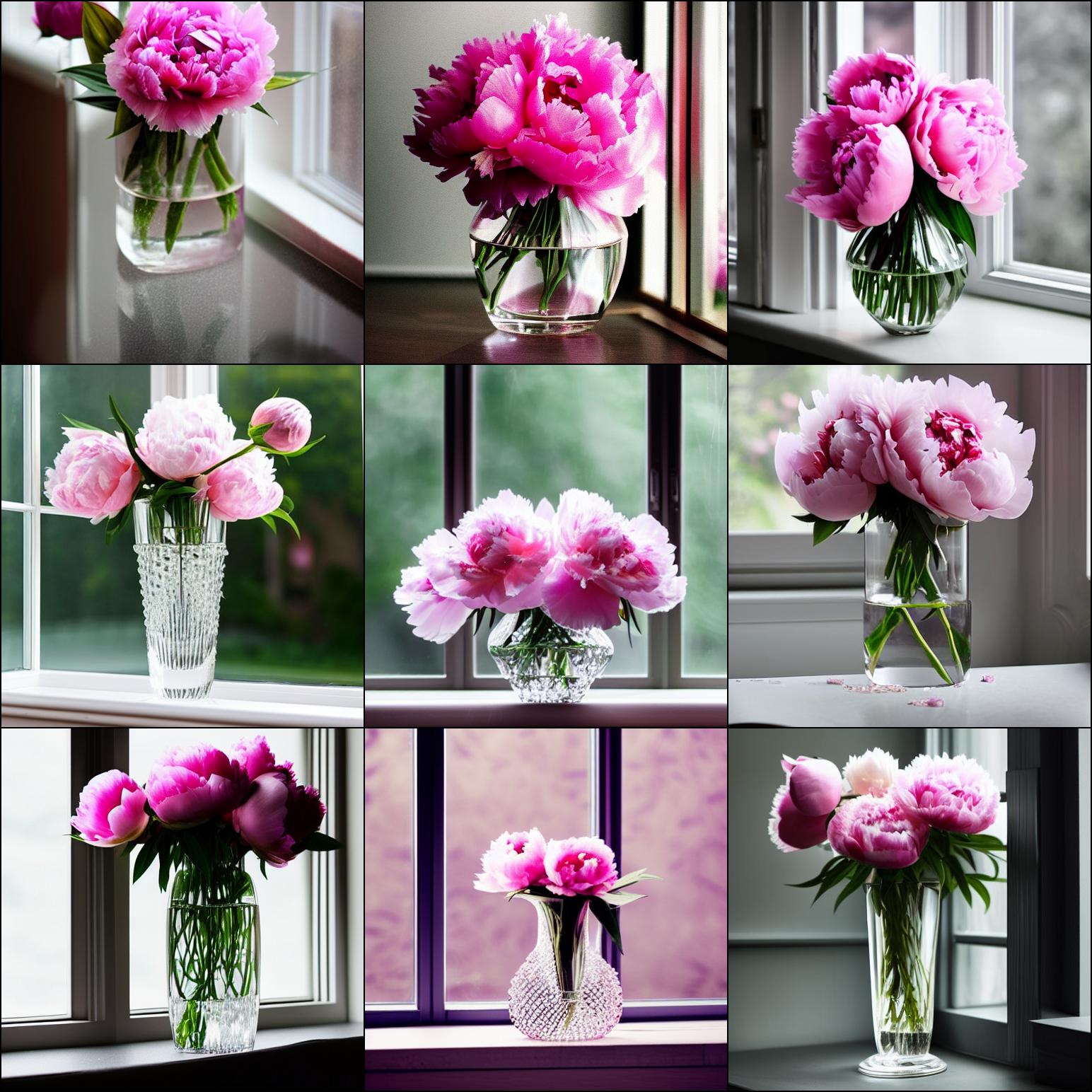
w/ CFG Guidance

Figure 4: Qualitative T2I comparison between vanilla conditional generation, GFT, and CFG on Stable Diffusion 1.5 with the prompt “Elegant crystal vase holding pink peonies, soft raindrops tracing paths down the window behind it”. More examples are in Figure 12.

5.1 Experimental Setups

Tasks & Models.

We evaluate GFT in both class-to-image (C2I) and text-to-image (T2I) tasks. For C2I, we experiment with diverse architectures: DiT (Peebles & Xie, 2023) (transformer-based latent diffusion model), MAR (Li et al., 2024) (masked-token prediction model with diffusion heads), and autoregressive models: VAR (Tian et al., 2024) and LlamaGen (Sun et al., 2024). For T2I, we use Stable Diffusion 1.5 (Rombach et al., 2022), a text-to-image model based on the U-Net architecture (Ronneberger et al., 2015), to provide a comprehensive evaluation of GFT’s performance across various conditioning modalities. All these models rely on guided sampling as a critical component.

Training & Evaluation.

We train C2I models on ImageNet-256x256 (Deng et al., 2009). For T2I models, we use a subset of the LAION-Aesthetic $5+$ (Schuhmann et al., 2022), consisting of 12.8 million image-text pairs. Our codebases are directly modified from the official CFG implementation of each respective baseline, keeping most hyperparameters consistent with CFG training. We use official OPENAI evaluation scripts to evaluate our C2I models. For T2I models, we evaluate our model on zero-shot COCO 2014 (Lin et al., 2014). The training and evaluation details for each model can be found in Appendix D.

5.2 Make CFG Models Guidance-Free

Method Effectiveness.

In Table 2 and 3, we apply GFT to fine-tune a wide spectrum of visual generative models. With less than 5% pretraining computation, the fine-tuned models achieve comparable FID scores to CFG while being 2× faster in sampling. Figure 4 visually demonstrates this quality improvement.

Comparison with other guidance-free approaches.

GFT achieves comparable performance to guidance distillation (designed for diffusion models) while outperforming AR alignment method in both performance (Table 2) and efficiency (Table 1). We attribute this effectiveness to GFT’s end-to-end training style, and to the nice convergence property of its maximum likelihood training objective.

Finetuning Efficiency

Figure 5 tracks the FID progression of DiT-XL/2 during fine-tuning. The guidance-free FID rapidly improves from 9.34 to 2.22 in the first epoch, followed by steady optimization. After three epochs, our model achieves a better FID than the CFG baseline (2.05 vs 2.11). This computational is almost negligible compared with pretraining, demonstrating GFT’s efficiency.

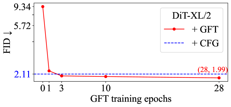
Figure 5: Efficient convergence of FID scores for GFT using DiT-XL/2 model across training epochs.

5.3 Building Guidance-Free Models from Scratch

Method	Guidance	DiT-B/2		MAR-B		LlamaGen-L		VAR-d16
		(Peebles & Xie, 2023)		(Li et al., 2024)		(Sun et al., 2024)		(Tian et al., 2024)
		FID $\downarrow$	IS $\uparrow$	FID $\downarrow$	IS $\uparrow$	FID $\downarrow$	IS $\uparrow$	FID $\downarrow$	IS $\uparrow$
Base	w/o	44.8	30.7	4.17	175.4	19.0	64.7	11.97	105.5
$\quad+$CFG	w/	9.72	161.5	2.27	260.7	3.06	257.1	3.36	280.1
$\quad+$GFT	w/o	10.9	128.5	2.39	264.7	2.88	238.4	3.28	251.3
GFT	w/o	9.04	166.6	2.27	279.5	2.52	270.5	3.42	254.8

Table 4: Performance comparison between GFT from-scratch training, CFG, and GFT fine-tuning variants across different model architectures. GFT and the base model are trained for the same number of epochs.

Training Guidance-Free Models from scratch is more tempting than the two-stage pipeline adopted by Sec 5.2. However, this is also more challenging due to higher requirements for the algorithm’s stability and convergence speed. We investigate this by comparing from-scratch GFT training with classic supervised training using CFG across various architectures, maintaining consistent training epochs. We mainly focus on smaller models due to computational constraints.

Performance.

Table 4 shows that GFT models trained from scratch outperform CFG baselines across DiT-B/2, MAR-B, and LlamaGen-L models, while reducing evaluation costs by 50%. Notably, these from-scratch models outperform their fine-tuned counterparts, demonstrating the advantages of direct guidance-free training.

Training stability.

An informative indicator of an algorithm’s stability and scalability is its loss convergence speed. With consistent hyperparameters, we find GFT convergences at least as fast as CFG for both diffusion and autoregressive modeling (Figure 6). Direct loss comparison is valid as both methods optimize the same objective: the conditional modeling loss for the dataset distribution. The only difference is that the conditional model for CFG is a single end-to-end model, while for GFT it is constructed as a linear interpolation of two model outputs.

Based on the above observations, we believe that GFT is at least as stable and reliable as CFG algorithms, providing a new training paradigm and a viable alternative for visual generative models.

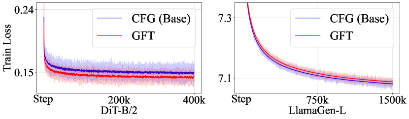
Figure 6: Comparison of training dynamics between GFT and CFG on diffusion and autoregressive models.

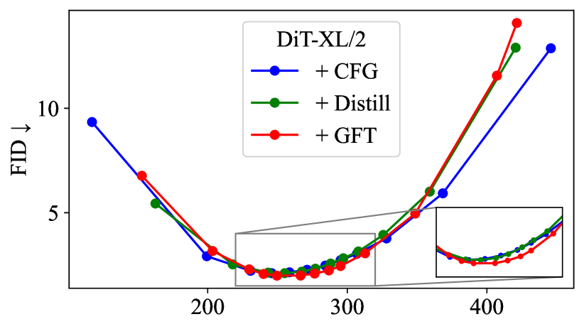
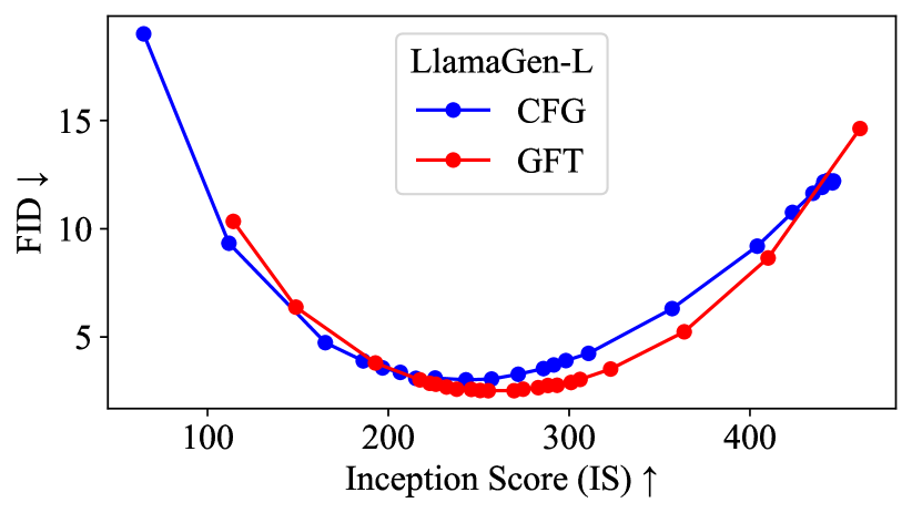
Figure 7: FID-IS trade-off comparisons on ImageNet. Upper: DiT-XL/2 with GFT (fine-tuned), CFG, and Guidance Distillation. Lower: LlamaGen-L with GFT (trained from scratch) and CFG.

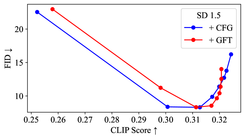
Figure 8: FID-CLIP trade-off comparison on COCO-2014 validation set. Methods compared using Stable Diffusion 1.5 (SD 1.5).

5.4 Sampling Temperature for Visual Generation

A key advantage of CFG is its flexible sampling temperature for diversity-fidelity trade-offs. Our results demonstrate that GFT models share this capability.

We evaluate diversity-fidelity trade-offs across various models, with FID-IS trade-off for c2i models and FID-CLIP trade-off for t2i models. Results for DiT-XL/2 (fine-tuning), LlamaGen-L (from-scratch training) and Stable Diffusion 1.5 (fine-tuning) are shown in Figures 7 and 8, with additional trade-off curves provided in Appendix C. For DiT-XL/2, we also compare GFT with Guidance Distillation, showing that GFT achieves results comparable to both CFG and Guidance Distillation in the diversity-fidelity trade-off.

Figure 1 shows how adjusting temperature $\beta$ produces effects similar to adjusting CFG’s scale $s$. This similarity results from both methods aiming to model the same distribution (Eq. 5). The key difference is that GFT directly learns a series of sampling distributions controlled by $\beta$ through training, while CFG modifies the sampling process to achieve comparable results.

6 Conclusion

In this work, we proposed Guidance-Free Training (GFT) as an alternative to guided sampling in visual generative models, achieving comparable performance to Classifier-Free Guidance (CFG). GFT reduces sampling computational costs by 50%. The method is simple to implement, requiring minimal modifications to existing codebases. Unlike previous distillation-based methods, GFT enables direct training from scratch.

Our extensive evaluation across multiple types of visual models demonstrates GFT’s effectiveness. The approach maintains high sample quality while offering flexible control over the diversity-fidelity trade-off through temperature adjustment. GFT represents an advancement in making high-quality visual generation more efficient and accessible.

Impact Statement

Our Guidance-Free Training (GFT) method significantly reduces the computational costs of visual generative models by eliminating the need for dual inference during sampling, contributing to more sustainable AI development and reduced environmental impact. However, since our method accelerates the sampling process of generative models, it could potentially be misused to create harmful content more efficiently, emphasizing the importance of establishing appropriate safety measures and deploying these models responsibly with proper oversight mechanisms.

Appendix A Related Work

Visual generation model with guidance.

Visual generative modeling has witnessed significant advancements in recent years. Recent explicit-likelihood approaches can be broadly categorized into diffusion-based models (Ho et al., 2020; Song et al., 2020b; Dhariwal & Nichol, 2021; Kingma et al., 2021; Rombach et al., 2022; Ramesh et al., 2022; Saharia et al., 2022; Karras et al., 2022; Bao et al., 2023; Peebles & Xie, 2023; Esser et al., 2024; Xie et al., 2024), auto-regressive models (Chen et al., 2020; Esser et al., 2021; Ramesh et al., 2021; Yu et al., 2021; Tian et al., 2024; Team, 2024; Sun et al., 2024; Ma et al., 2024; Zhang et al., 2024; Tang et al., 2024), and masked-prediction models (Chang et al., 2022; Yu et al., 2023a; Chang et al., 2023; Li et al., 2024; Yu et al., 2024; Fan et al., 2024). The introduction of guidance techniques has substantially improved the capabilities of these models. These include classifier guidance (Dhariwal & Nichol, 2021), classifier-free guidance (Ho & Salimans, 2022), energy guidance (Chung et al., 2022; Zhao et al., 2022; Lu et al., 2023; Song et al., 2023), and various advanced guidance methods (Kynkäänniemi et al., 2024; Karras et al., 2024; Chung et al., 2024; Koulischer et al., ; Shenoy et al., 2024).

Guidance distillation.

To address the computational overhead introduced by classifier-free guidance (CFG), One widely used approach to remove CFG is guidance distillation (Meng et al., 2023), where a student model is trained to directly learn the output of a pre-trained teacher model that incorporates guidance. This idea of guidance distillation has been widely adopted in methods aimed at accelerating diffusion models (Luo et al., 2023; Yin et al., 2024b, a; Zhou et al., 2024). By integrating the teacher model’s guided outputs into the training process, these approaches achieve efficient few-step generation without guidance.

Condition Contrastive Alignment.

Beyond guidance distillation, Condition Contrastive Alignment (CCA) (Chen et al., 2024b) could also significantly enhance the guidance-free performance of visual AR models through alignment (Rafailov et al., 2023; Chen et al., 2024a) in a self-contrastive manner.

Appendix B Proof of Theorem 1

We first copy the training objective in Eq. 3.2 and Eq. 8.

$${\mathcal{L}}_{\theta}^{\text{raw}}=\mathbb{E}_{p({\bm{x}},{\bm{c}}),t,\bm{\epsilon},\beta}\left[\|\beta\epsilon_{\theta}^{s}({\bm{x}}_{t}|{\bm{c}},\beta)+(1-\beta)\epsilon_{\theta}^{u}({\bm{x}}_{t})-\bm{\epsilon}\|_{2}^{2}\right].$$ (15)

$${\mathcal{L}}_{\theta}^{\text{practical}}=\mathbb{E}_{p({\bm{x}},{\bm{c}}_{\varnothing}),t,\bm{\epsilon},\beta}\|\beta\epsilon_{\theta}^{s}({\bm{x}}_{t}|{\bm{c}}_{\varnothing},\beta)+(1-\beta)\mathrm{\mathbf{sg}}[\epsilon_{\theta}^{u}({\bm{x}}_{t}|\varnothing,1)]-\bm{\epsilon}\|_{2}^{2}.$$ (16)

Theorem 1 (GFT Optimal Solution).

Given unlimited model capacity and training data, the optimal $\epsilon_{\theta^{*}}^{s}$ for optimizing Eq. 15 and Eq. 16 are the same. Both satisfy

$$\epsilon_{\theta^{*}}^{s}({\bm{x}}_{t}|{\bm{c}},\beta)=-\sigma_{t}\left[\frac{1}{\beta}\nabla_{{\bm{x}}_{t}}\log p_{t}({\bm{x}}_{t}|{\bm{c}})-(\frac{1}{\beta}-1)\nabla_{{\bm{x}}_{t}}\log p_{t}({\bm{x}}_{t})\right]$$

Proof.

The proof is quite straightforward.

First consider the unconditional part of the model. Let $\beta=1$ in ${\mathcal{L}}_{\theta}^{\text{raw}}$, we have

$${\mathcal{L}}_{\theta}^{\text{raw}}=\mathbb{E}_{p({\bm{x}},{\bm{c}}),t,\bm{\epsilon},\beta=1}\left[\|\epsilon_{\theta}^{u}({\bm{x}}_{t})-\bm{\epsilon}\|_{2}^{2}\right],$$

which is standard unconditional diffusion loss. According to Eq. 2 we have

$$\epsilon_{\theta^{*}}^{u}({\bm{x}}_{t})=-\sigma_{t}\nabla_{{\bm{x}}_{t}}\log p_{t}({\bm{x}}_{t})$$ (17)

Then we prove stopping the unconditional gradient does not change this optimal solution. Taking derivatives of ${\mathcal{L}}_{\theta}^{\text{practical}}$ we have:

$$\nabla_{\theta}{\mathcal{L}}_{\theta}^{\text{practical}}({\bm{c}}_{\varnothing}=\varnothing) =\mathbb{E}_{p({\bm{x}}),t,\bm{\epsilon},\beta}\nabla_{\theta}\|\beta\epsilon_{\theta}^{s}({\bm{x}}_{t}|\varnothing,1)+(1-\beta)\mathrm{\mathbf{sg}}[\epsilon_{\theta}^{u}({\bm{x}}_{t}|\varnothing,1)]-\bm{\epsilon}\|_{2}^{2}$$

$$=\mathbb{E}_{p({\bm{x}}),t,\bm{\epsilon},\beta}2\beta[\nabla_{\theta}\epsilon_{\theta}^{s}({\bm{x}}_{t}|\varnothing,1)]\|\beta\epsilon_{\theta}^{s}({\bm{x}}_{t}|\varnothing,1)+(1-\beta)\epsilon_{\theta}^{u}({\bm{x}}_{t}|\varnothing,1)-\bm{\epsilon}\|_{2}$$

$$=\mathbb{E}_{p({\bm{x}}),t,\bm{\epsilon},\beta}2\beta[\nabla_{\theta}\epsilon_{\theta}^{s}({\bm{x}}_{t}|\varnothing,1)]\|\epsilon_{\theta}^{s}({\bm{x}}_{t}|\varnothing,1)-\bm{\epsilon}\|_{2}$$

$$=[2\mathbb{E}\beta]\nabla_{\theta}\mathbb{E}_{p({\bm{x}},{\bm{c}}),t,\bm{\epsilon},\beta=1}\left[\|\epsilon_{\theta}^{u}({\bm{x}}_{t})-\bm{\epsilon}\|_{2}^{2}\right]$$

$$=[2\mathbb{E}\beta]\nabla_{\theta}{\mathcal{L}}_{\theta}^{\text{raw}}(\beta=1)$$

Since $[2\mathbb{E}\beta]$ is a constant, this does not change the convergence point of ${\mathcal{L}}_{\theta}^{\text{raw}}$. The optimal unconditional solution for ${\mathcal{L}}_{\theta}^{\text{practical}}$ remains the same.

For the conditional part of the model, since both ${\mathcal{L}}_{\theta}^{\text{raw}}$ and ${\mathcal{L}}_{\theta}^{\text{practical}}$ are standard conditional diffusion loss, we have

$$\beta\epsilon_{\theta^{*}}^{s}({\bm{x}}_{t}|{\bm{c}},\beta)+(1-\beta)\epsilon_{\theta^{*}}^{u}({\bm{x}}_{t})=-\sigma_{t}\nabla_{{\bm{x}}_{t}}\log p_{t}({\bm{x}}_{t}|{\bm{c}})$$

Combining Eq. 17, we have

$$\epsilon_{\theta^{*}}^{s}({\bm{x}}_{t}|{\bm{c}},\beta)=-\sigma_{t}\left[\frac{1}{\beta}\nabla_{{\bm{x}}_{t}}\log p_{t}({\bm{x}}_{t}|{\bm{c}})-(\frac{1}{\beta}-1)\nabla_{{\bm{x}}_{t}}\log p_{t}({\bm{x}}_{t})\right].$$

Let $s=\frac{1}{\beta}-1$, we can see that GFT models the same sampling distribution as CFG (Eq. 4). ∎

Appendix C Additional Experiment Results.

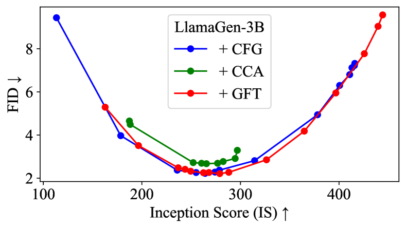
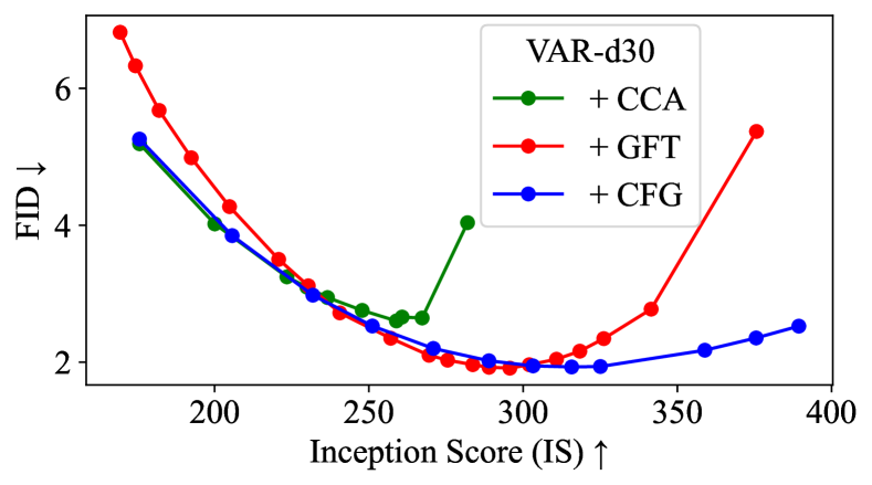
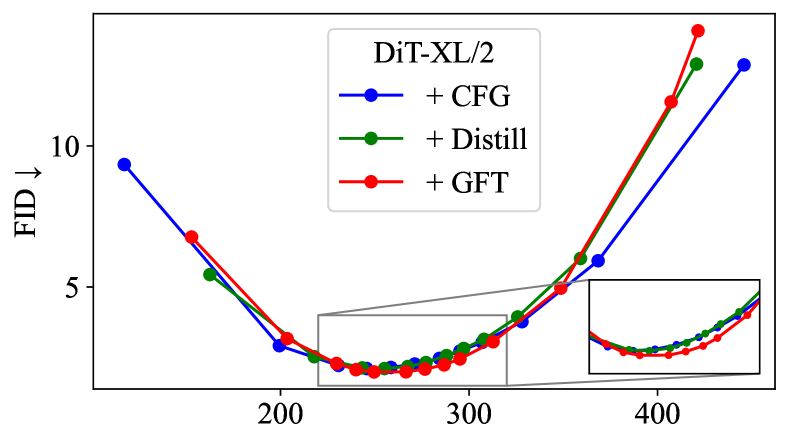
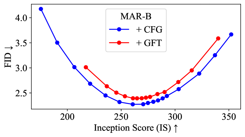
Figure 9: FID-IS trade-off comparison in fine-tuning experiments.

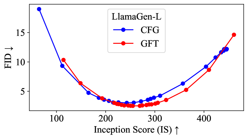
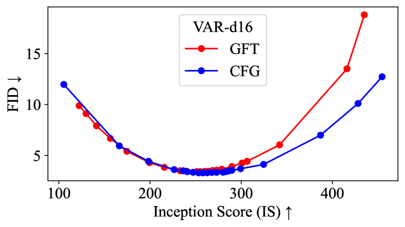
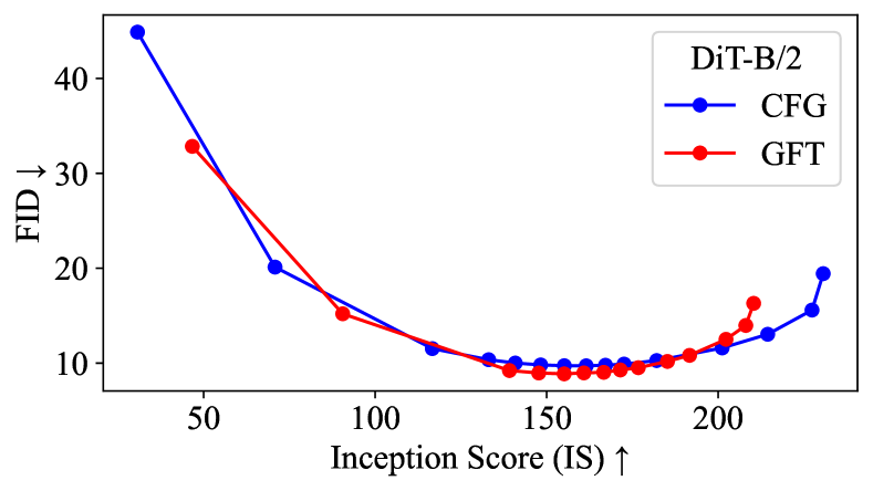
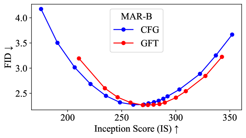
Figure 10: FID-IS trade-off comparison in from-scratch-training experiments.

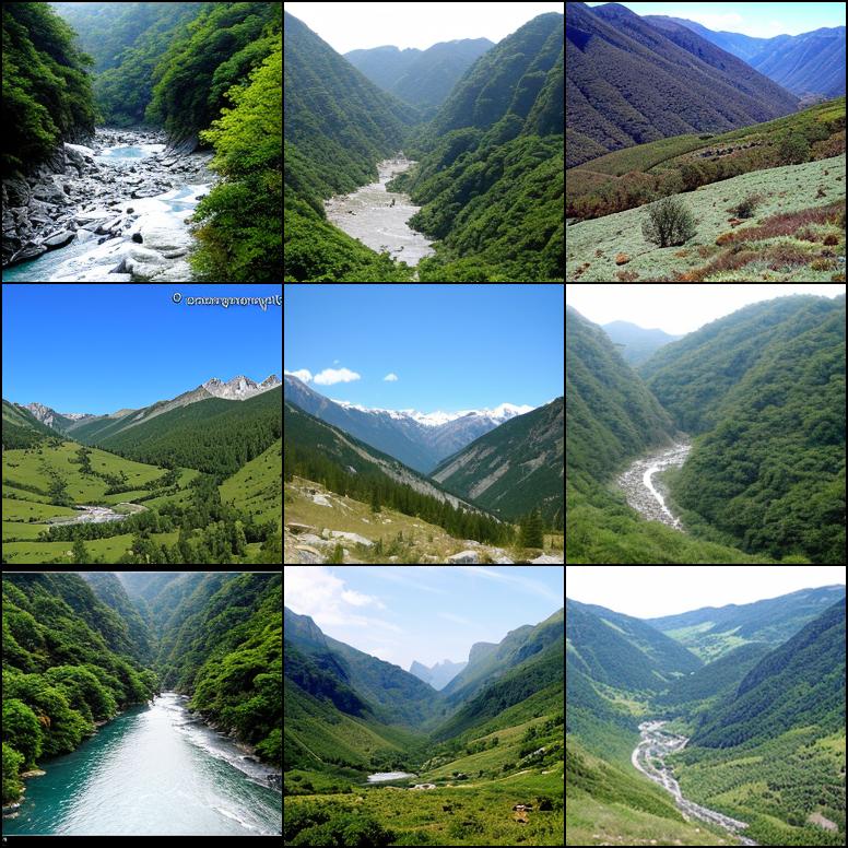
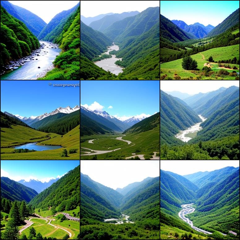
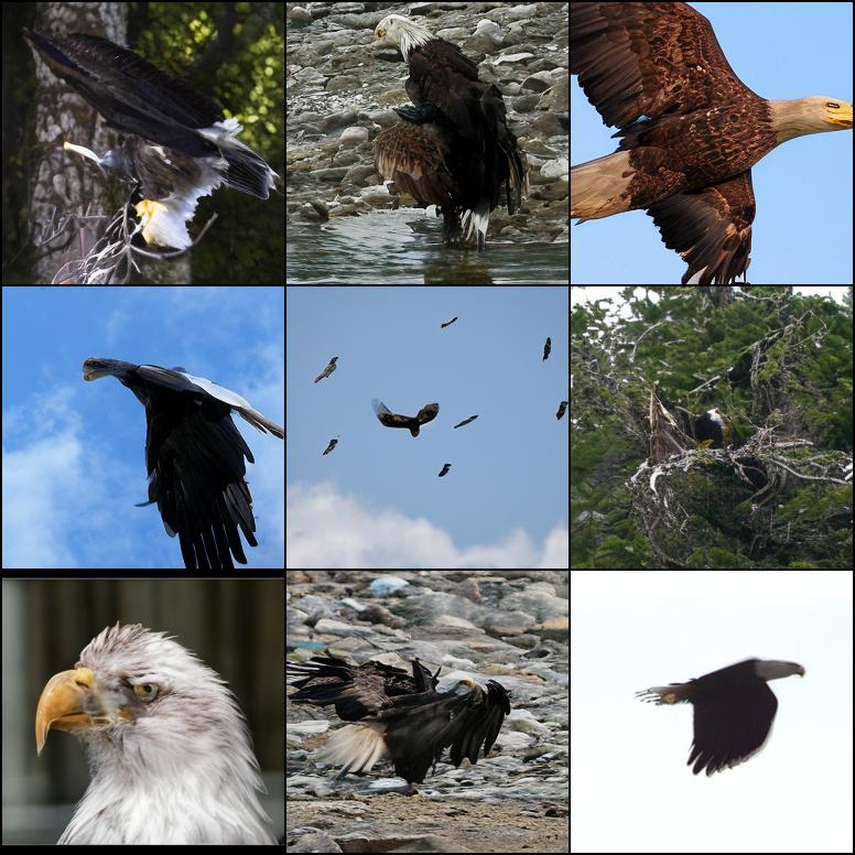
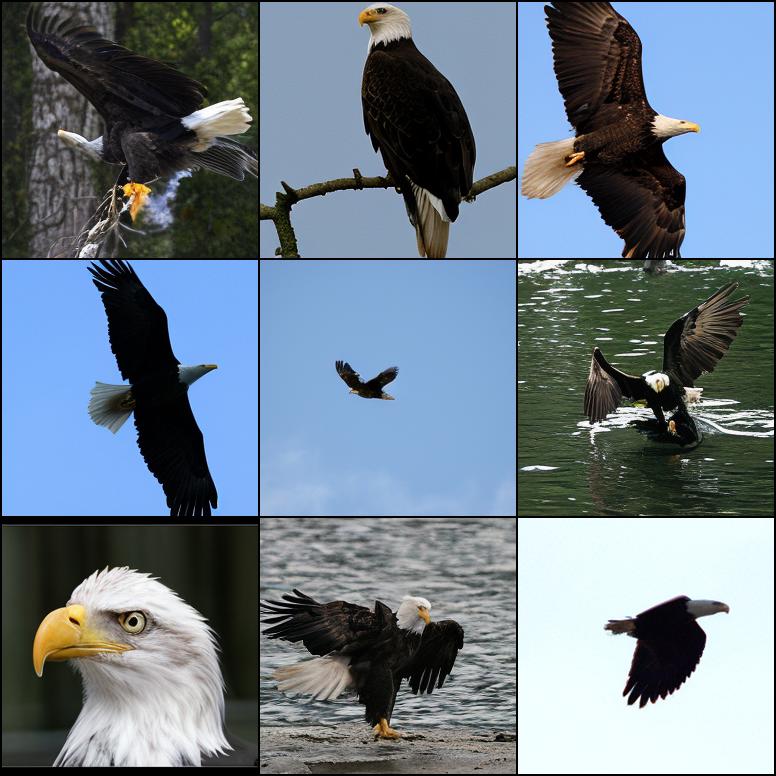
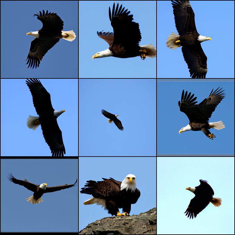
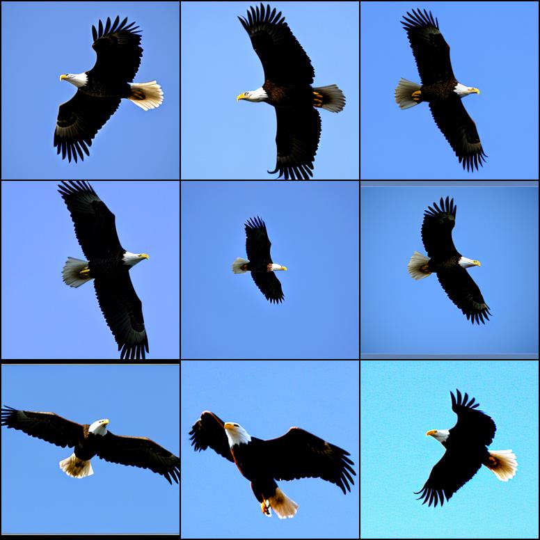
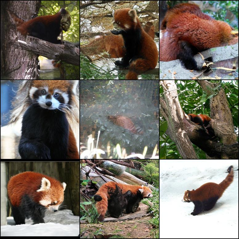
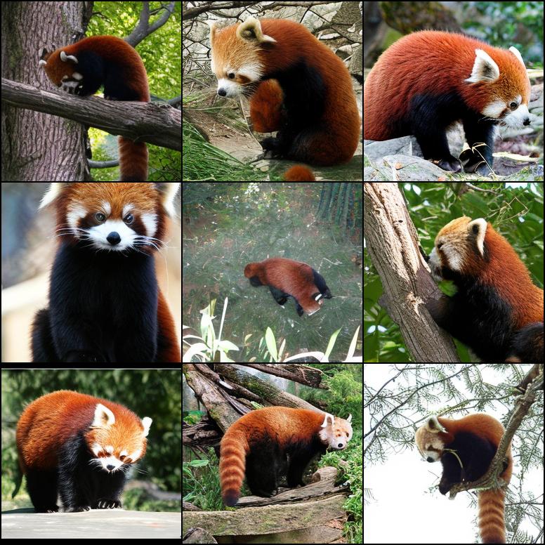
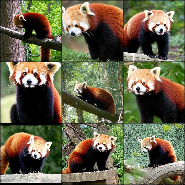
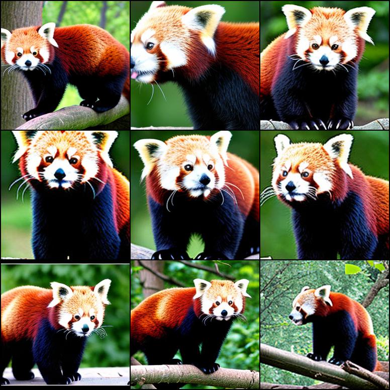
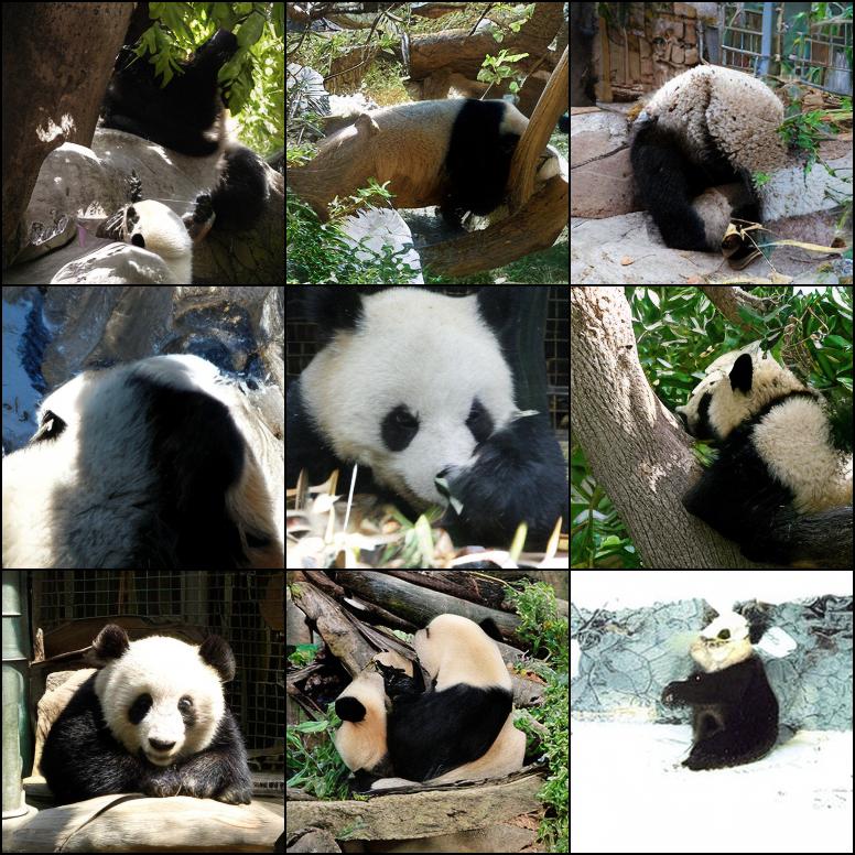
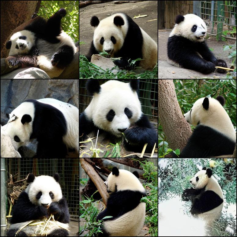
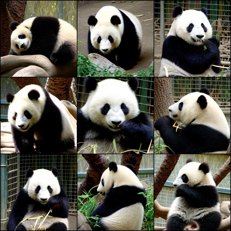
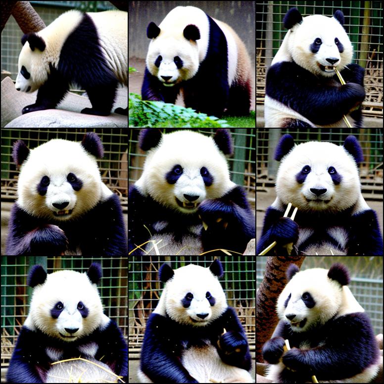
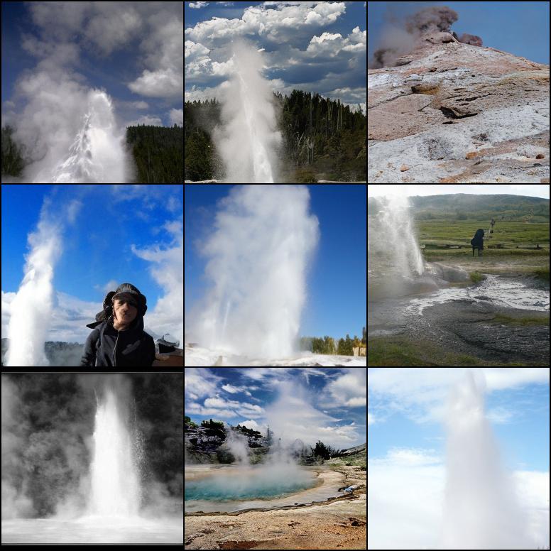
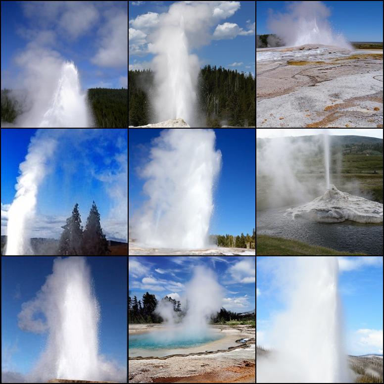
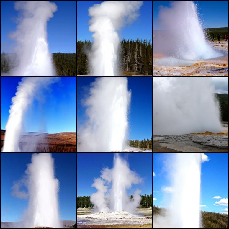
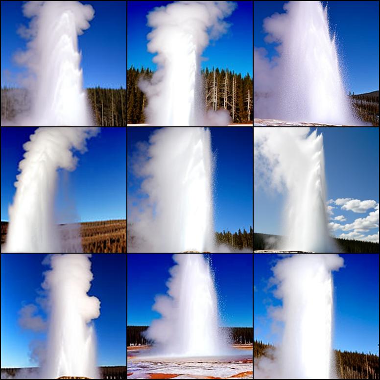
$\beta=1.0$

$\beta=0.5$

$\beta=0.25$

$\beta=0.1$

Figure 11: Additional results of temperature sampling ($\beta$) impact on DiT-XL/2 after applying GFT.

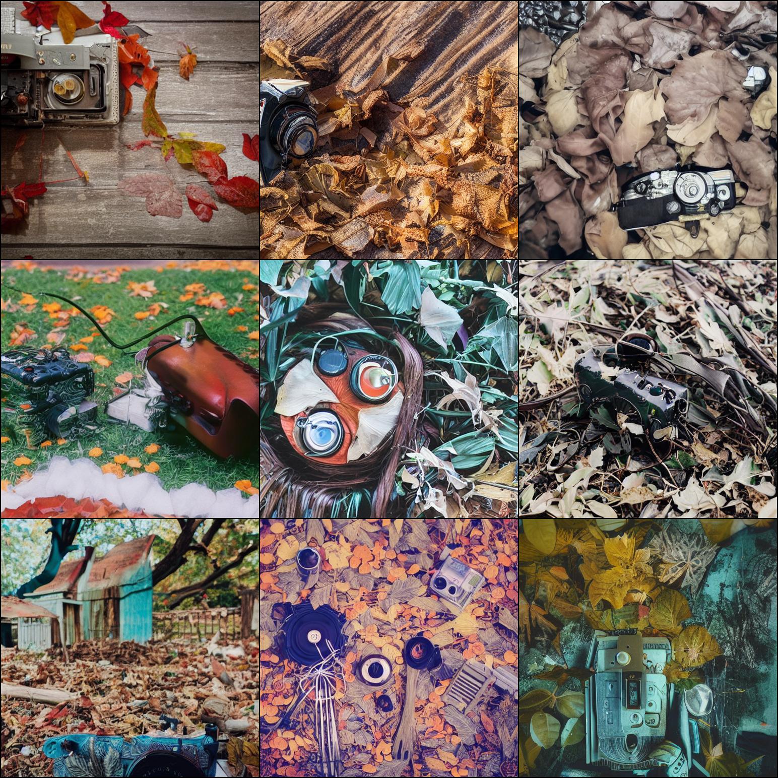
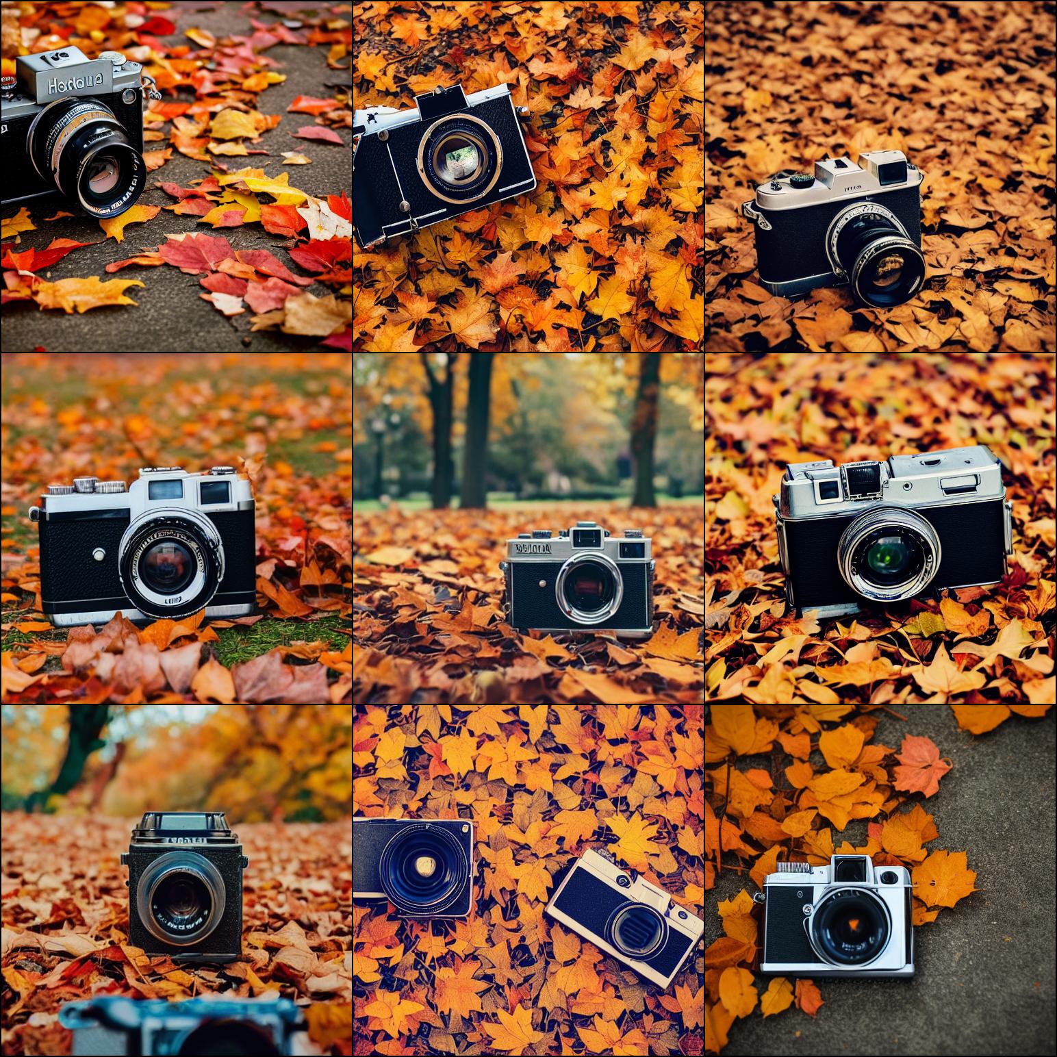
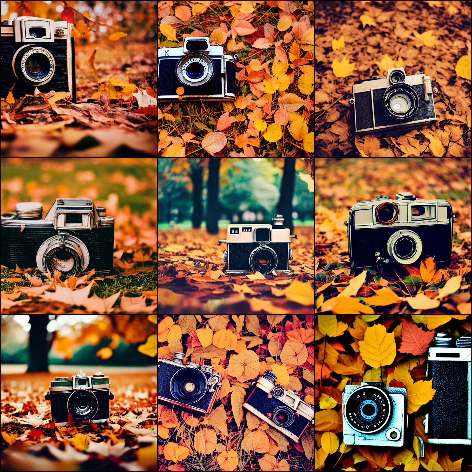
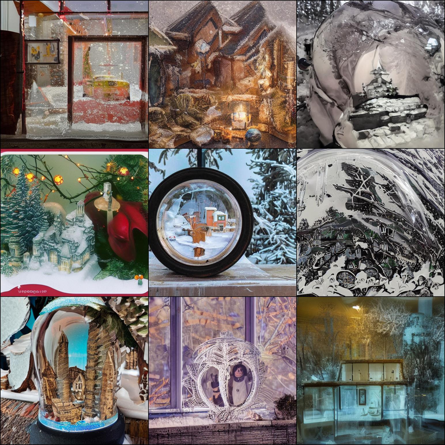
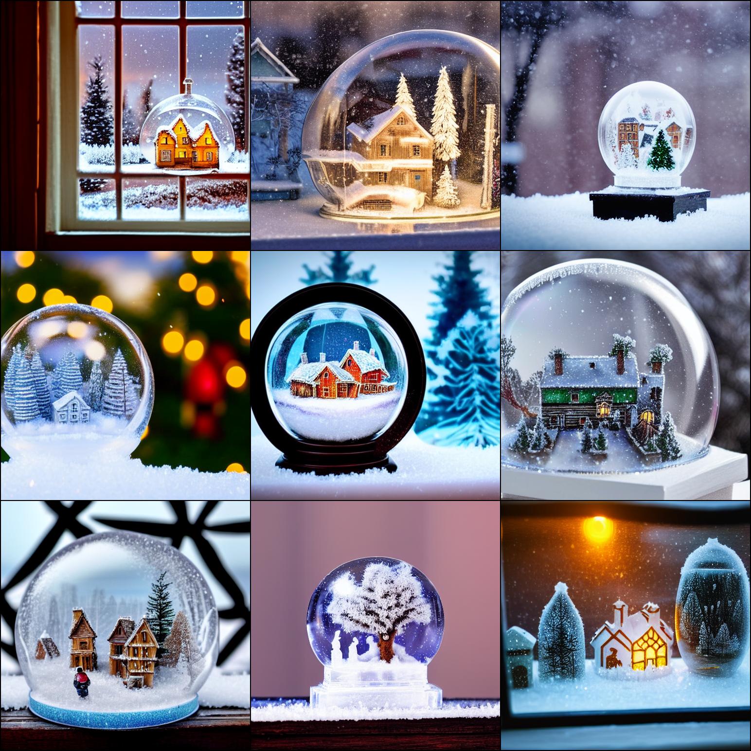
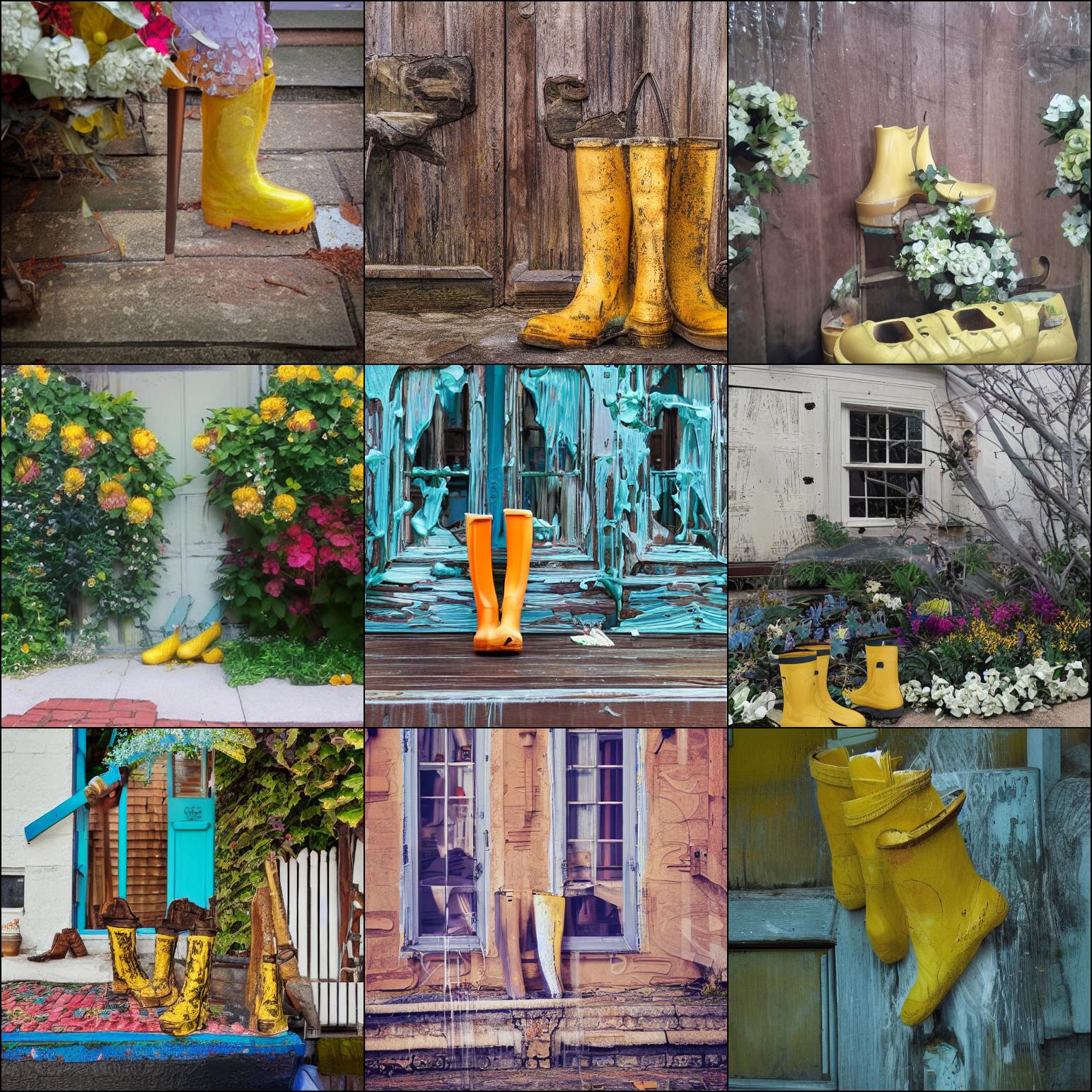
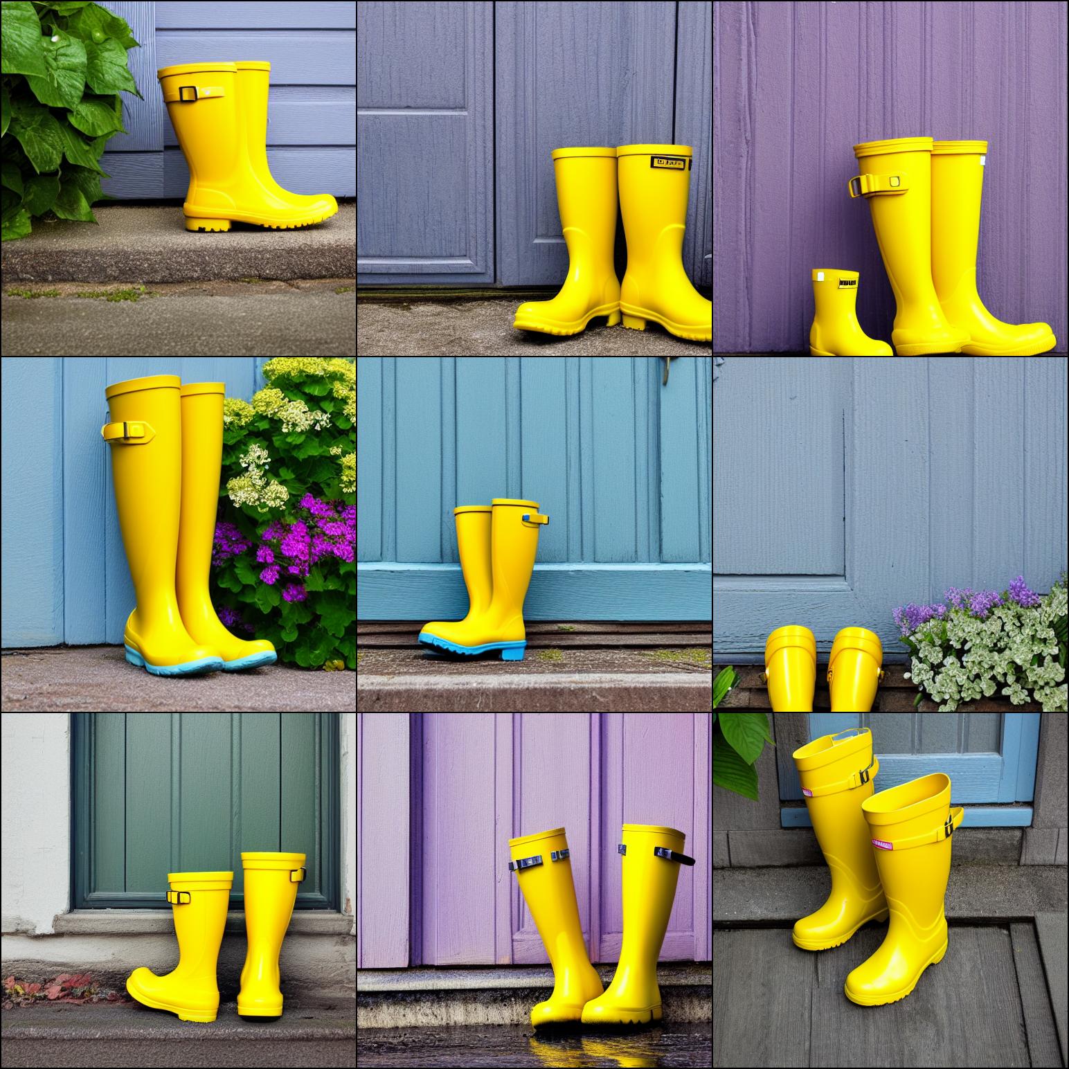
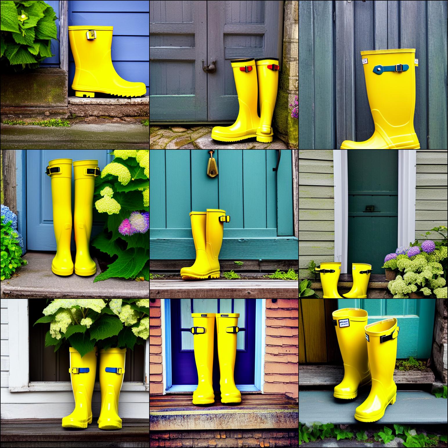
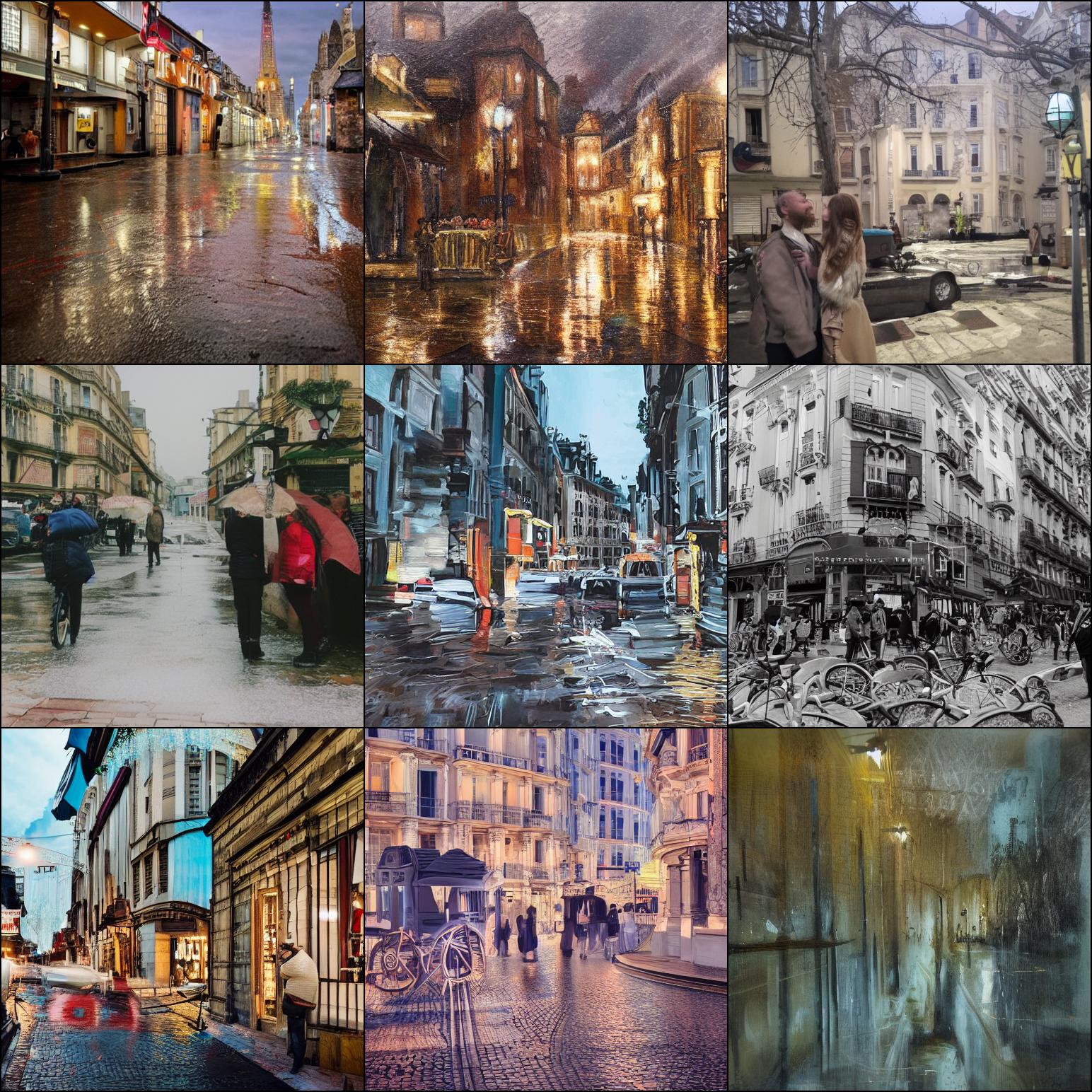
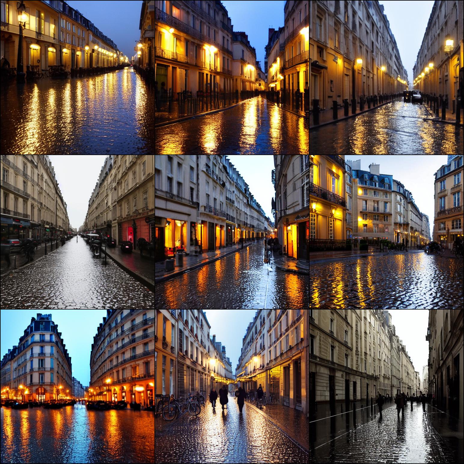
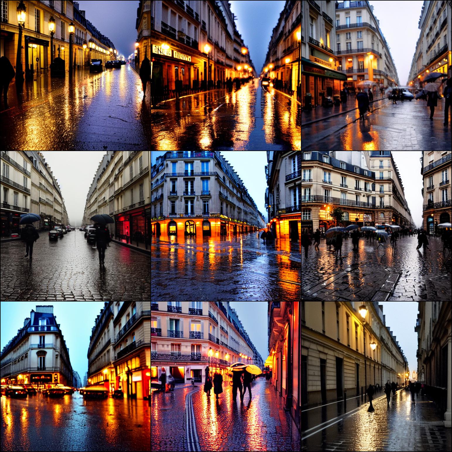
w/o Guidance

GFT (w/o Guidance)

w/ CFG Guidance

Figure 12: Additional results of qualitative T2I comparison between vanilla conditional generation, GFT, and CFG on Stable Diffusion 1.5.

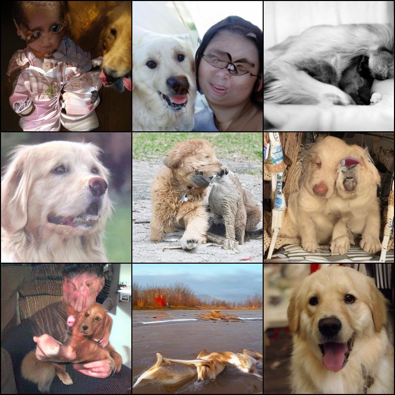
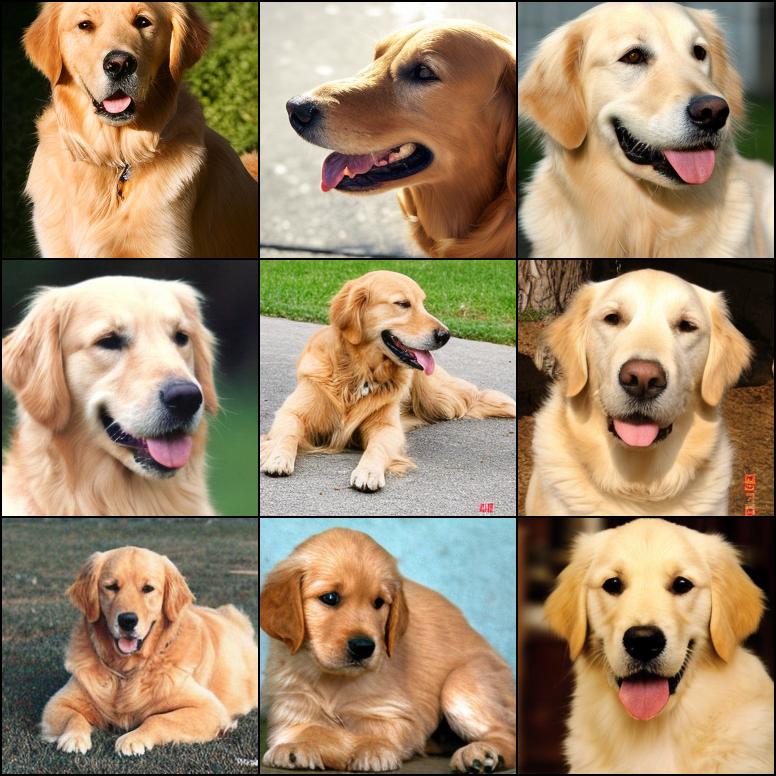
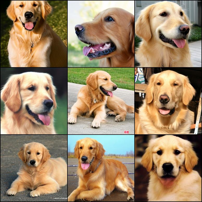
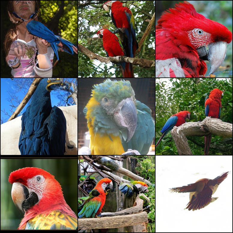
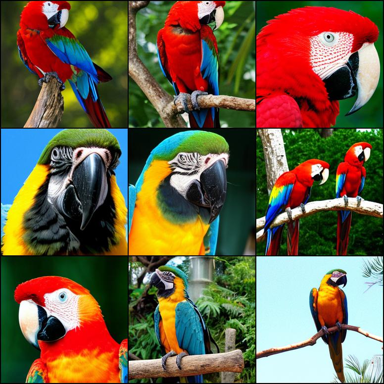
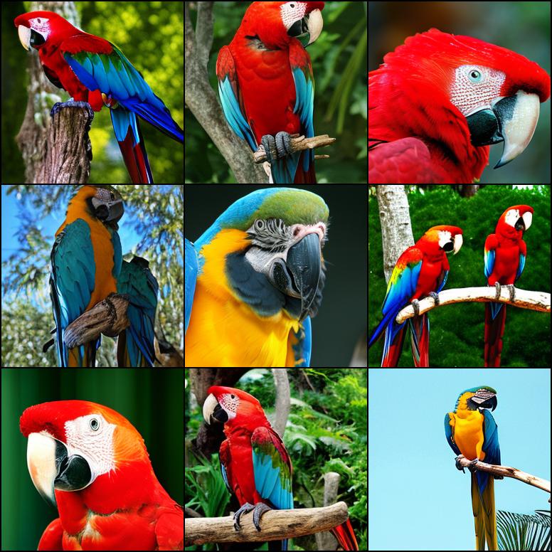
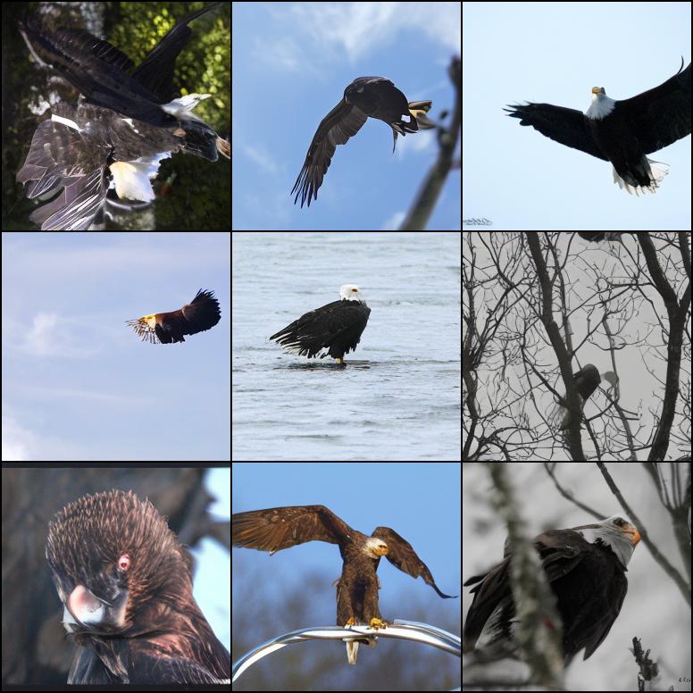
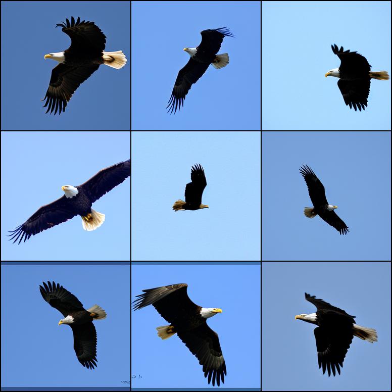
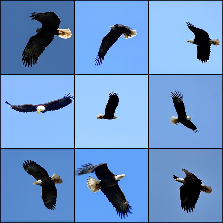
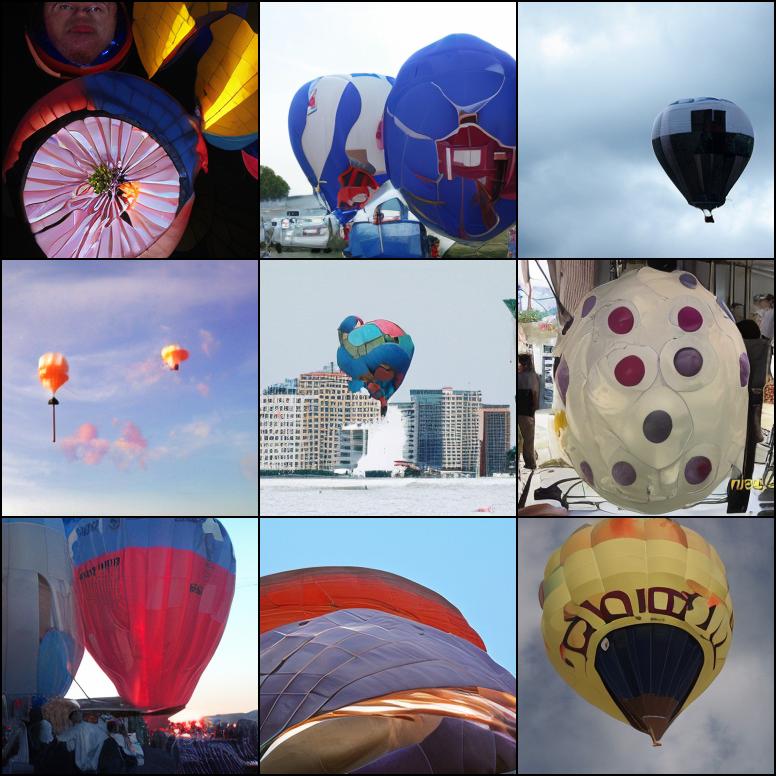
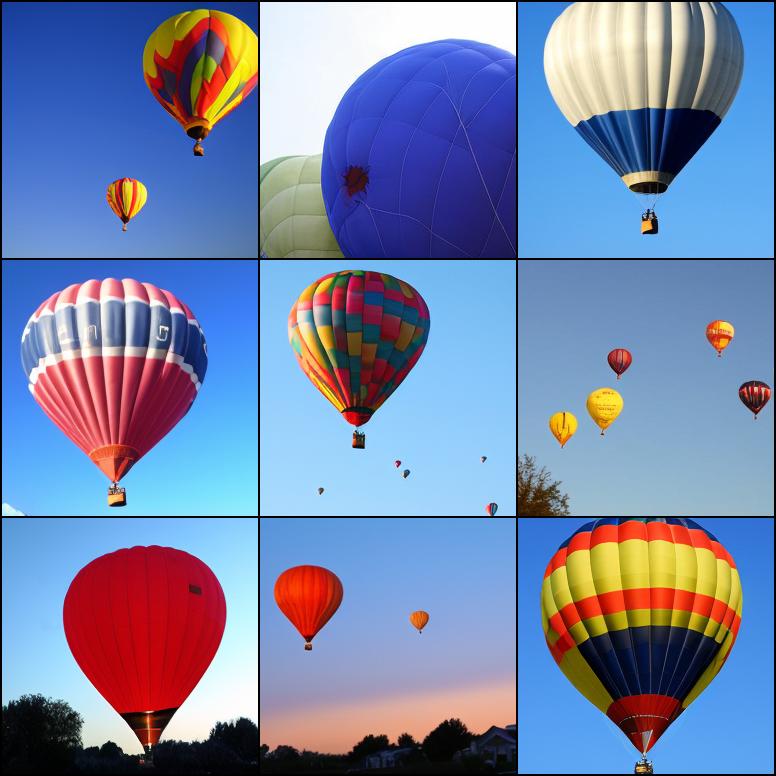
w/o Guidance

GFT (w/o Guidance)

w/ CFG Guidance

Figure 13: Additional results of qualitative C2I comparison between vanilla conditional generation, GFT, and CFG on DiT-XL/2.

Appendix D Implementation Details.

For all models, we keep training hyperparameters and other design choices consistent with their official codebases if not otherwise stated. We employ a mix of H100, A100 and A800 GPU cards for experimentation.

DiT.

We mainly apply GFT to fine-tune DiT-XL/2 (28 epochs, 2% of pretraining epochs) and train DiT-B/2 from scratch (80 epochs, following the original DiT paper’s settings (Peebles & Xie, 2023)). Since the DiT-B/2 pretraining checkpoint is not publicly available, we reproduce its pretraining experiment. For all experiments, we use a batch size of 256 and a learning rate of $1e-4$. For DiT-XL/2 fine-tuning experiments, we employ a cosine-decay learning rate scheduler.

For comparison, we also fine-tune DiT-XL/2 using guidance distillation, with a scale range from 1 to 5, while keeping all other hyperparameters aligned with GFT.

The original DiT uses the old-fashioned DDPM (Ho et al., 2020) which learns both the mean and variance, while GFT is only concerned about the mean. We therefore abandon the variance output channels and related losses during training and switch to the Dpm-solver++ (Lu et al., 2022) sampler with 50 steps at inference. For reference, our baseline, DiT-XL/2 with CFG, achieves an FID of 2.11 using DPM-solver++, compared with 2.27 reported in the original paper. All results are evaluated with EMA models. The EMA decay rate is set to 0.9999.

VAR.

We mainly apply GFT to fine-tune VAR-d30 models (15 epochs) or train VAR-d16 models from scratch (200 epochs). Batch size is 768. The initial learning rate is $1e-5$ in fine-tuning experiments and $1e-4$ in pretraining experiments. Following VAR (Tian et al., 2024), we employ a learning rate scheduler including a warmup and a linear decay process (minimal is 1% of the initial).

VAR by default adopts a pyramid CFG technique on predicted logits. The guidance scale $0$ decreases linearly during the decoding process. Specifically, let n be the current decoding step index, and N be the total steps. The $n$-step guidance scale $s_{n}$ is

$$s_{n}=\frac{n}{N-1}s_{0}.$$

We find pyramid CFG is crucial to an ideal performance of VAR, and thus design a similar pyramid $\beta$ schedule during training:

$$\beta_{n}=\left[(\frac{n}{N-1})^{\alpha}(\frac{1}{\beta_{0}}-1)+1\right]^{-1},$$

where $\beta_{n}$ represents the token-specific $\beta$ value applied in the GFT AR loss (Eq. 12). $\alpha\geq 0$ is a hyperparameter to be tuned.

When $\alpha=0$, we have $\beta_{n}=\beta_{0}$, standing for standard GFT. When $\alpha=1.0$, we have $\frac{1}{\beta_{n}}-1=(\frac{n}{N-1})(\frac{1}{\beta_{0}}-1)$, corresponding to the default pyramid CFG technique applied by VAR. In practice, we set $\alpha=1.5$ in GFT training and find this slightly outperforms $\alpha=1.0$.

LlamaGen.

We mainly apply GFT to fine-tune LlamaGen-3B models (15 epochs) or train LlamaGen-L models from scratch (300 epochs). For fine-tuning, the batch size is 256, and the learning rate is $2e-4$. For pretraining, the batch size is 768, and the learning rate is $1e-4$. We adopt a cosine-decay learning rate scheduler in all experiments.

MAR.

We apply GFT to MAR-B, including both fine-tuning (10 epochs) and training from scratch (800 epochs). We find the batch size crucial for MAR and use 2048 following the original paper. For fine-tuning, we employ a learning rate scheduler including a 5-epoch linear warmup to $8e-4$ and a cosine decay process to $1e-4$. For training from scratch, we employ a 100-epoch linear lr warmup to $8e-4$, followed by a constant lr schedule, which is the same configuration as the original MAR pretraining.

The original MAR follows the old-fashioned DDPM (Ho et al., 2020) which learns both the mean and variance, while GFT is only concerned about the mean. We therefore abandon the variance output channels and related losses during training and switch to the DDIM (Song et al., 2020a) sampler with 100 steps at inference. As the $\beta$ condition may not precisely capture the effects of the guidance scale after training, we tune the inference $\beta$ schedule to maximize the performance. Specifically, we adopt a power-cosine schedule

$$\beta_{n}=\left[\frac{1-\cos((n/(N-1))^{\alpha}\pi)}{2}(\frac{1}{\beta_{0}}-1)+1\right]^{-1}$$

where we choose $\alpha=0.4$.

Stable Diffusion 1.5.

We apply GFT to fine-tune Stable Diffusion 1.5 (SD1.5) (Rombach et al., 2022) for 50,000 gradient updates with a batch size of 256 and constant learning rate of $1e-5$ with 1,000 warmup steps. We disable conditioning dropout as we find it improves CLIP score.

For evaluation, following GigaGAN (Kang et al., 2023) and DMD (Yin et al., 2024b), we generate images using 30K prompts from the COCO2014 (Lin et al., 2014) validation set, downsample them to 256×256, and compare with 40,504 real images from the same validation set. We use clean-FID (Parmar et al., 2022) to calculate FID and OpenCLIP-G (Ilharco et al., 2021; Cherti et al., 2023) to calculate CLIP score (Radford et al., 2021). All results are evaluated using 50 steps DPM-solver++ (Lu et al., 2022) with EMA models. The EMA decay rate is set to 0.999 for insufficient training steps.

Appendix E Prompts for Figure 12

We use the following prompts for Figure 12.

• A vintage camera in a park, autumn leaves scattered around it.

• Pristine snow globe showing a winter village scene, sitting on a frost-covered pine windowsill at dawn.

• Vibrant yellow rain boots standing by a cottage door, fresh raindrops dripping from blooming hydrangeas.

• Rain-soaked Parisian streets at twilight.

References

- Bao et al. (2023) Bao, F., Nie, S., Xue, K., Cao, Y., Li, C., Su, H., and Zhu, J. All are worth words: A vit backbone for diffusion models. In Proceedings of the IEEE/CVF conference on computer vision and pattern recognition, pp. 22669–22679, 2023.
- Black et al. (2023) Black, K., Janner, M., Du, Y., Kostrikov, I., and Levine, S. Training diffusion models with reinforcement learning. arXiv preprint arXiv:2305.13301, 2023.
- Chang et al. (2022) Chang, H., Zhang, H., Jiang, L., Liu, C., and Freeman, W. T. Maskgit: Masked generative image transformer. In Proceedings of the IEEE/CVF Conference on Computer Vision and Pattern Recognition, pp. 11315–11325, 2022.
- Chang et al. (2023) Chang, H., Zhang, H., Barber, J., Maschinot, A., Lezama, J., Jiang, L., Yang, M.-H., Murphy, K., Freeman, W. T., Rubinstein, M., et al. Muse: Text-to-image generation via masked generative transformers. arXiv preprint arXiv:2301.00704, 2023.
- Chen et al. (2024a) Chen, H., He, G., Su, H., and Zhu, J. Noise contrastive alignment of language models with explicit rewards. Advances in neural information processing systems, 2024a.
- Chen et al. (2024b) Chen, H., Su, H., Sun, P., and Zhu, J. Toward guidance-free ar visual generation via condition contrastive alignment. arXiv preprint arXiv:2410.09347, 2024b.
- Chen et al. (2020) Chen, M., Radford, A., Child, R., Wu, J., Jun, H., Luan, D., and Sutskever, I. Generative pretraining from pixels. In International conference on machine learning, pp. 1691–1703. PMLR, 2020.
- Cherti et al. (2023) Cherti, M., Beaumont, R., Wightman, R., Wortsman, M., Ilharco, G., Gordon, C., Schuhmann, C., Schmidt, L., and Jitsev, J. Reproducible scaling laws for contrastive language-image learning. In Proceedings of the IEEE/CVF Conference on Computer Vision and Pattern Recognition, pp. 2818–2829, 2023.
- Chung et al. (2022) Chung, H., Kim, J., Mccann, M. T., Klasky, M. L., and Ye, J. C. Diffusion posterior sampling for general noisy inverse problems. arXiv preprint arXiv:2209.14687, 2022.
- Chung et al. (2024) Chung, H., Kim, J., Park, G. Y., Nam, H., and Ye, J. C. Cfg++: Manifold-constrained classifier free guidance for diffusion models. arXiv preprint arXiv:2406.08070, 2024.
- Deng et al. (2009) Deng, J., Dong, W., Socher, R., Li, L.-J., Li, K., and Fei-Fei, L. Imagenet: A large-scale hierarchical image database. In 2009 IEEE conference on computer vision and pattern recognition, pp. 248–255. Ieee, 2009.
- Dhariwal & Nichol (2021) Dhariwal, P. and Nichol, A. Diffusion models beat gans on image synthesis. Advances in neural information processing systems, 34:8780–8794, 2021.
- Esser et al. (2021) Esser, P., Rombach, R., and Ommer, B. Taming transformers for high-resolution image synthesis. In Proceedings of the IEEE/CVF conference on computer vision and pattern recognition, pp. 12873–12883, 2021.
- Esser et al. (2024) Esser, P., Kulal, S., Blattmann, A., Entezari, R., Müller, J., Saini, H., Levi, Y., Lorenz, D., Sauer, A., Boesel, F., Podell, D., Dockhorn, T., English, Z., Lacey, K., Goodwin, A., Marek, Y., and Rombach, R. Scaling rectified flow transformers for high-resolution image synthesis, 2024.
- Fan et al. (2024) Fan, L., Li, T., Qin, S., Li, Y., Sun, C., Rubinstein, M., Sun, D., He, K., and Tian, Y. Fluid: Scaling autoregressive text-to-image generative models with continuous tokens. arXiv preprint arXiv:2410.13863, 2024.
- Gao et al. (2023) Gao, S., Zhou, P., Cheng, M.-M., and Yan, S. Masked diffusion transformer is a strong image synthesizer. In Proceedings of the IEEE/CVF International Conference on Computer Vision, pp. 23164–23173, 2023.
- Ho & Salimans (2022) Ho, J. and Salimans, T. Classifier-free diffusion guidance. arXiv preprint arXiv:2207.12598, 2022.
- Ho et al. (2020) Ho, J., Jain, A., and Abbeel, P. Denoising diffusion probabilistic models. Advances in neural information processing systems, 33:6840–6851, 2020.
- Ilharco et al. (2021) Ilharco, G., Wortsman, M., Carlini, N., Taori, R., Dave, A., Shankar, V., Namkoong, H., Miller, J., Hajishirzi, H., Farhadi, A., and Schmidt, L. Openclip, July 2021. URL https://doi.org/10.5281/zenodo.5143773.
- Kang et al. (2023) Kang, M., Zhu, J.-Y., Zhang, R., Park, J., Shechtman, E., Paris, S., and Park, T. Scaling up gans for text-to-image synthesis. In Proceedings of the IEEE/CVF Conference on Computer Vision and Pattern Recognition, pp. 10124–10134, 2023.
- Karras et al. (2022) Karras, T., Aittala, M., Aila, T., and Laine, S. Elucidating the design space of diffusion-based generative models. Advances in neural information processing systems, 35:26565–26577, 2022.
- Karras et al. (2024) Karras, T., Aittala, M., Kynkäänniemi, T., Lehtinen, J., Aila, T., and Laine, S. Guiding a diffusion model with a bad version of itself. arXiv preprint arXiv:2406.02507, 2024.
- Kingma et al. (2021) Kingma, D., Salimans, T., Poole, B., and Ho, J. Variational diffusion models. Advances in neural information processing systems, 34:21696–21707, 2021.
- (24) Koulischer, F., Deleu, J., Raya, G., Demeester, T., and Ambrogioni, L. Dynamic negative guidance of diffusion models: Towards immediate content removal. In Neurips Safe Generative AI Workshop 2024.
- Kynkäänniemi et al. (2024) Kynkäänniemi, T., Aittala, M., Karras, T., Laine, S., Aila, T., and Lehtinen, J. Applying guidance in a limited interval improves sample and distribution quality in diffusion models. arXiv preprint arXiv:2404.07724, 2024.
- Langley (2000) Langley, P. Crafting papers on machine learning. In Langley, P. (ed.), Proceedings of the 17th International Conference on Machine Learning (ICML 2000), pp. 1207–1216, Stanford, CA, 2000. Morgan Kaufmann.
- Lee et al. (2022) Lee, D., Kim, C., Kim, S., Cho, M., and Han, W.-S. Autoregressive image generation using residual quantization. In Proceedings of the IEEE/CVF Conference on Computer Vision and Pattern Recognition, pp. 11523–11532, 2022.
- Li et al. (2023) Li, T., Chang, H., Mishra, S., Zhang, H., Katabi, D., and Krishnan, D. Mage: Masked generative encoder to unify representation learning and image synthesis. In Proceedings of the IEEE/CVF Conference on Computer Vision and Pattern Recognition, pp. 2142–2152, 2023.
- Li et al. (2024) Li, T., Tian, Y., Li, H., Deng, M., and He, K. Autoregressive image generation without vector quantization. arXiv preprint arXiv:2406.11838, 2024.
- Lin et al. (2014) Lin, T.-Y., Maire, M., Belongie, S., Hays, J., Perona, P., Ramanan, D., Dollár, P., and Zitnick, C. L. Microsoft coco: Common objects in context. In Computer Vision–ECCV 2014: 13th European Conference, Zurich, Switzerland, September 6-12, 2014, Proceedings, Part V 13, pp. 740–755. Springer, 2014.
- Lu et al. (2022) Lu, C., Zhou, Y., Bao, F., Chen, J., Li, C., and Zhu, J. Dpm-solver++: Fast solver for guided sampling of diffusion probabilistic models. arXiv preprint arXiv:2211.01095, 2022.
- Lu et al. (2023) Lu, C., Chen, H., Chen, J., Su, H., Li, C., and Zhu, J. Contrastive energy prediction for exact energy-guided diffusion sampling in offline reinforcement learning. In International Conference on Machine Learning, pp. 22825–22855. PMLR, 2023.
- Luo et al. (2023) Luo, S., Tan, Y., Huang, L., Li, J., and Zhao, H. Latent consistency models: Synthesizing high-resolution images with few-step inference. arXiv preprint arXiv:2310.04378, 2023.
- Ma et al. (2024) Ma, X., Zhou, M., Liang, T., Bai, Y., Zhao, T., Chen, H., and Jin, Y. Star: Scale-wise text-to-image generation via auto-regressive representations. arXiv preprint arXiv:2406.10797, 2024.
- Meng et al. (2023) Meng, C., Rombach, R., Gao, R., Kingma, D., Ermon, S., Ho, J., and Salimans, T. On distillation of guided diffusion models. In Proceedings of the IEEE/CVF Conference on Computer Vision and Pattern Recognition (CVPR), pp. 14297–14306, June 2023.
- Nichol et al. (2021) Nichol, A., Dhariwal, P., Ramesh, A., Shyam, P., Mishkin, P., McGrew, B., Sutskever, I., and Chen, M. Glide: Towards photorealistic image generation and editing with text-guided diffusion models. arXiv preprint arXiv:2112.10741, 2021.
- Parmar et al. (2022) Parmar, G., Zhang, R., and Zhu, J.-Y. On aliased resizing and surprising subtleties in gan evaluation. In Proceedings of the IEEE/CVF Conference on Computer Vision and Pattern Recognition, pp. 11410–11420, 2022.
- Peebles & Xie (2023) Peebles, W. and Xie, S. Scalable diffusion models with transformers. In Proceedings of the IEEE/CVF International Conference on Computer Vision, pp. 4195–4205, 2023.
- Radford et al. (2021) Radford, A., Kim, J. W., Hallacy, C., Ramesh, A., Goh, G., Agarwal, S., Sastry, G., Askell, A., Mishkin, P., Clark, J., et al. Learning transferable visual models from natural language supervision. In International conference on machine learning, pp. 8748–8763. PMLR, 2021.
- Rafailov et al. (2023) Rafailov, R., Sharma, A., Mitchell, E., Manning, C. D., Ermon, S., and Finn, C. Direct preference optimization: Your language model is secretly a reward model. In Thirty-seventh Conference on Neural Information Processing Systems, 2023.
- Ramesh et al. (2021) Ramesh, A., Pavlov, M., Goh, G., Gray, S., Voss, C., Radford, A., Chen, M., and Sutskever, I. Zero-shot text-to-image generation. In International Conference on Machine Learning, pp. 8821–8831. PMLR, 2021.
- Ramesh et al. (2022) Ramesh, A., Dhariwal, P., Nichol, A., Chu, C., and Chen, M. Hierarchical text-conditional image generation with clip latents. arXiv preprint arXiv:2204.06125, 1(2):3, 2022.
- Rombach et al. (2022) Rombach, R., Blattmann, A., Lorenz, D., Esser, P., and Ommer, B. High-resolution image synthesis with latent diffusion models. In Proceedings of the IEEE/CVF conference on computer vision and pattern recognition, pp. 10684–10695, 2022.
- Ronneberger et al. (2015) Ronneberger, O., Fischer, P., and Brox, T. U-net: Convolutional networks for biomedical image segmentation. In Medical image computing and computer-assisted intervention–MICCAI 2015: 18th international conference, Munich, Germany, October 5-9, 2015, proceedings, part III 18, pp. 234–241. Springer, 2015.
- Saharia et al. (2022) Saharia, C., Chan, W., Saxena, S., Li, L., Whang, J., Denton, E. L., Ghasemipour, K., Gontijo Lopes, R., Karagol Ayan, B., Salimans, T., et al. Photorealistic text-to-image diffusion models with deep language understanding. Advances in Neural Information Processing Systems, 35:36479–36494, 2022.
- Schuhmann et al. (2022) Schuhmann, C., Beaumont, R., Vencu, R., Gordon, C., Wightman, R., Cherti, M., Coombes, T., Katta, A., Mullis, C., Wortsman, M., et al. Laion-5b: An open large-scale dataset for training next generation image-text models. Advances in Neural Information Processing Systems, 35:25278–25294, 2022.
- Shenoy et al. (2024) Shenoy, R., Pan, Z., Balakrishnan, K., Cheng, Q., Jeon, Y., Yang, H., and Kim, J. Gradient-free classifier guidance for diffusion model sampling. arXiv preprint arXiv:2411.15393, 2024.
- Song et al. (2020a) Song, J., Meng, C., and Ermon, S. Denoising diffusion implicit models. arXiv preprint arXiv:2010.02502, 2020a.
- Song et al. (2023) Song, J., Zhang, Q., Yin, H., Mardani, M., Liu, M.-Y., Kautz, J., Chen, Y., and Vahdat, A. Loss-guided diffusion models for plug-and-play controllable generation. In International Conference on Machine Learning, pp. 32483–32498. PMLR, 2023.
- Song et al. (2020b) Song, Y., Sohl-Dickstein, J., Kingma, D. P., Kumar, A., Ermon, S., and Poole, B. Score-based generative modeling through stochastic differential equations. arXiv preprint arXiv:2011.13456, 2020b.
- Song et al. (2021) Song, Y., Durkan, C., Murray, I., and Ermon, S. Maximum likelihood training of score-based diffusion models. Advances in neural information processing systems, 34:1415–1428, 2021.
- Sun et al. (2024) Sun, P., Jiang, Y., Chen, S., Zhang, S., Peng, B., Luo, P., and Yuan, Z. Autoregressive model beats diffusion: Llama for scalable image generation. arXiv preprint arXiv:2406.06525, 2024.
- Tang et al. (2024) Tang, H., Wu, Y., Yang, S., Xie, E., Chen, J., Chen, J., Zhang, Z., Cai, H., Lu, Y., and Han, S. Hart: Efficient visual generation with hybrid autoregressive transformer. arXiv preprint arXiv:2410.10812, 2024.
- Team (2024) Team, C. Chameleon: Mixed-modal early-fusion foundation models. arXiv preprint arXiv:2405.09818, 2024.
- Tian et al. (2024) Tian, K., Jiang, Y., Yuan, Z., Peng, B., and Wang, L. Visual autoregressive modeling: Scalable image generation via next-scale prediction. arXiv preprint arXiv:2404.02905, 2024.
- Xie et al. (2024) Xie, J., Mao, W., Bai, Z., Zhang, D. J., Wang, W., Lin, K. Q., Gu, Y., Chen, Z., Yang, Z., and Shou, M. Z. Show-o: One single transformer to unify multimodal understanding and generation. arXiv preprint arXiv:2408.12528, 2024.
- Yin et al. (2024a) Yin, T., Gharbi, M., Park, T., Zhang, R., Shechtman, E., Durand, F., and Freeman, W. T. Improved distribution matching distillation for fast image synthesis. arXiv preprint arXiv:2405.14867, 2024a.
- Yin et al. (2024b) Yin, T., Gharbi, M., Zhang, R., Shechtman, E., Durand, F., Freeman, W. T., and Park, T. One-step diffusion with distribution matching distillation. In Proceedings of the IEEE/CVF Conference on Computer Vision and Pattern Recognition, pp. 6613–6623, 2024b.
- Yu et al. (2021) Yu, J., Li, X., Koh, J. Y., Zhang, H., Pang, R., Qin, J., Ku, A., Xu, Y., Baldridge, J., and Wu, Y. Vector-quantized image modeling with improved vqgan. arXiv preprint arXiv:2110.04627, 2021.
- Yu et al. (2023a) Yu, L., Cheng, Y., Sohn, K., Lezama, J., Zhang, H., Chang, H., Hauptmann, A. G., Yang, M.-H., Hao, Y., Essa, I., et al. Magvit: Masked generative video transformer. In Proceedings of the IEEE/CVF Conference on Computer Vision and Pattern Recognition, pp. 10459–10469, 2023a.
- Yu et al. (2023b) Yu, L., Lezama, J., Gundavarapu, N. B., Versari, L., Sohn, K., Minnen, D., Cheng, Y., Gupta, A., Gu, X., Hauptmann, A. G., et al. Language model beats diffusion–tokenizer is key to visual generation. arXiv preprint arXiv:2310.05737, 2023b.
- Yu et al. (2024) Yu, Q., Weber, M., Deng, X., Shen, X., Cremers, D., and Chen, L.-C. An image is worth 32 tokens for reconstruction and generation. arXiv preprint arXiv:2406.07550, 2024.
- Zhang et al. (2024) Zhang, Q., Dai, X., Yang, N., An, X., Feng, Z., and Ren, X. Var-clip: Text-to-image generator with visual auto-regressive modeling. arXiv preprint arXiv:2408.01181, 2024.
- Zhao et al. (2022) Zhao, M., Bao, F., Li, C., and Zhu, J. Egsde: Unpaired image-to-image translation via energy-guided stochastic differential equations. Advances in Neural Information Processing Systems, 35:3609–3623, 2022.
- Zhou et al. (2024) Zhou, M., Wang, Z., Zheng, H., and Huang, H. Long and short guidance in score identity distillation for one-step text-to-image generation. arXiv preprint arXiv:2406.01561, 2024.