Constraining Disk-to-Corona Power Transfer Fraction, Soft X-ray Excess Origin, and Black Hole Spin Population of Type-1 AGN across Mass Scales

Abstract

Understanding the nature of the accretion disk, its interplay with the X-ray corona, and assessing black hole spin demographics are some open challenges in astrophysics. In this work, we examine the predictions of the standard $\alpha$-disk model, origin of the soft X-ray excess, and measure the black hole spin parameter by applying the updated high-density disk reflection model to the XMM-Newton/NuSTAR broadband (0.3$-$78 keV) X-ray spectra of a sample of Type-1 AGN. Our Bayesian analysis confirms that the high-density relativistic reflection model with a broken power-law emissivity profile can simultaneously fit the soft X-ray excess, broad iron K line, and Compton hump for $\sim$70% of the sample, while an additional warm Comptonization model is still required to describe the observed soft X-ray excess for the remaining sources. Our first-ever calculation of the disk-to-corona power transfer fraction reveals that the fraction of power released from the accretion disk into the hot corona can have diverse values, the sample median of which is $0.7_{-0.4}^{+0.2}$. We find that the transferred power from the accretion disk can potentially soften the X-ray spectrum of the hot corona. The median values of the hot coronal temperature and optical depth for the sample are estimated to be $63_{-11}^{+23}$ keV and $0.85_{-0.27}^{+0.12}$, respectively. Finally, through joint XMM-Newton+NuSTAR relativistic reflection spectroscopy, we systematically constrain the black hole spin parameter across the broad range of black hole masses, $\log(M_{\rm BH}/M_{\odot})\sim 5.5-9.0$, and increase the available spin measurements in the AGN population by $\sim$20%.

1 Introduction

Active galactic nuclei (AGN) are the most luminous ($10^{41}-10^{48}~{\rm erg~s^{-1}}$), compact regions at the center of galaxies, fed by mass accretion from their host galaxies onto supermassive black holes (SMBHs) of mass $M_{\rm BH}\sim 10^{5-10}M_{\odot}$ (e.g. Lynden-Bell 1969; Gurzadian & Ozernoi 1979; Rees 1984; Reines et al. 2013). The gradual loss of angular momentum causes the inflowing matter to move toward the center of gravity, forming an accretion disk around the SMBH, which is believed to be the engine that powers AGN (e.g. Frank et al. 2002). The observed correlation between SMBH mass and host-galaxy bulge velocity dispersion (e.g. Ferrarese & Merritt 2000; Gültekin et al. 2009; Kormendy & Ho 2013) implies that the growth of the host galaxy is coupled with the energy output from the central SMBH, and feedback from AGN can play a key role in the evolution of galaxies (e.g. Di Matteo et al. 2005; Hopkins & Elvis 2010; Fabian 2012; Heckman & Best 2014). Indeed, the AGN accretion disk can influence the evolution of the host galaxy via a sustained release of gravitational energy in the form of radiation or outflows (e.g. Silk & Rees 1998; Tombesi et al. 2011; Parker et al. 2017; Pinto et al. 2018). However, understanding the nature and dynamics of the accretion disk remains an open question in both theoretical and observational astrophysics.

AGN are inherently multi-wavelength phenomena (Elvis et al., 1994), and their spectral energy distributions (SEDs) at different energies are the outcome of various physical processes arising from distinct regions, dominating the observed emission for different AGN sub-classes. However, the most effective way to probe the immediate vicinity of the central SMBH or innermost regions of AGN is to study the X-ray emission from Type-1 AGN, the line of sight of which is not obscured by the molecular torus (e.g. Pier & Krolik 1993; Cappi et al. 2006; Combes et al. 2019). In the unified view of AGN (Antonucci, 1993; Netzer, 2015), the primary X-ray emission is produced by Compton up-scattering of the optical/UV seed photons in an optically thin, hot plasma (Sunyaev & Titarchuk, 1980; Haardt & Maraschi, 1993) called ‘corona’ surrounding the SMBH as also suggested by the global radiation magnetohydrodynamic (MHD) simulations (Jiang et al., 2019b), where the seed photons are thought to be supplied by the accretion disk (Page & Thorne, 1974). However, it is not well known how the accretion disk and corona are coupled and what fraction of power from the accretion disk gets transported into the corona. When this coronal radiation illuminates the accretion disk, it produces an intrinsic reflection spectrum containing a forest of fluorescent emission lines below $\sim 2$ keV, narrow iron (Fe) K emission lines (K_α/K_β), and a Compton scattering hump above $10$ keV (George & Fabian, 1991; Ross & Fabian, 2005; García & Kallman, 2010). If the disk is close to the black hole, the intrinsic reflection spectrum gets smeared by the strong gravitational field and produces the blurred or relativistic reflection spectrum containing a soft X-ray excess below around 1$-$2 keV, a broad Fe K emission line (6$-$7 keV), and the Compton hump (15$-$30 keV) (e.g. Fabian et al. 2000; García et al. 2014; Matt et al. 2014). Currently, relativistic reflection spectroscopy of the innermost accretion disk is the only means of measuring massive black hole spins in AGN (e.g. Brenneman & Reynolds 2006; Reynolds 2021; Bambi et al. 2021; Mallick et al. 2022), which is crucial for studying the formation and growth channels of SMBHs (e.g. Volonteri et al. 2005; Berti & Volonteri 2008; Volonteri et al. 2013; Pacucci & Loeb 2020). Thus, it is of central importance to model the disk reflection signatures precisely and assess the demographics of black hole spin in AGN.

The origin of the soft X-ray excess observed below $\sim$ 1$-$2 keV in AGN is still unknown despite its discovery nearly 40 years ago by Singh et al. (1985) and Arnaud et al. (1985). At first, it was thought to be the high-energy tail of the standard disk emission. However, the soft excess temperature is much higher than the maximum disk temperature and remains constant within the range of $\sim$ 0.1$-$0.3 keV, irrespective of the black hole mass (see Gierliński & Done 2004 for high-mass quasars and Mallick et al. 2022 for low-mass dwarf AGN).

Currently, two models are used to describe the soft X-ray excess emission. One model requires low-temperature Comptonization of optical/UV disk photons in an optically thick, warm corona (e.g. Mallick et al. 2017; Petrucci et al. 2018; Chalise et al. 2022). On the other hand, the reflection model naturally produces soft X-ray excess as relativistically smeared, broadened fluorescent lines arising from the innermost accretion disk (e.g. Crummy et al. 2006; García et al. 2014; Mallick & Dewangan 2018). However, in some AGN, relativistic reflection alone cannot model the entire soft X-ray excess, and a warm Comptonization component is still required, particularly when the density of the accretion disk is fixed at the canonical value of $n_{\rm e}=10^{15}~\rm{cm}^{-3}$ (e.g. Ark 120: Mallick et al. 2017; Porquet et al. 2018, Mrk 110: Porquet et al. 2024). This issue was tackled by employing a high-density disk reflection model (García et al., 2016), which can potentially fit the entire soft X-ray excess by boosting the strength of the excess emission below $\sim$1 keV in the model, where the density parameter can reach as high as $\log[n_{\rm e}/\rm{cm}^{-3}]=20$, first implemented by Mallick et al. (2022). For a geometrically thin and optically thick standard accretion disk (Shakura & Sunyaev 1973; hereafter SS73), the gas density of the inner disk is likely to be higher than $10^{15}$ cm^-3. Moreover, the theoretical work of Svensson & Zdziarski (1994) (hereafter SZ94) proposed that the inner disk density would be even higher than that predicted by the SS73 model after including the fraction of power transferred from the accretion disk to the corona, i.e., the disk-to-corona power transfer fraction. While higher-density disk reflection has become more prevalent in explaining the origin of the soft X-ray excess in AGN (Mallick et al., 2018; García et al., 2019; Mallick et al., 2022), the disk-to-corona power transfer fraction has yet to be explored.

In this paper, we study the broadband (0.3$-$78 keV) spectra of a sample of Type-1 AGN across the central SMBH mass scales of $M_{\rm BH}\approx 10^{5.5-9}M_{\rm\odot}$, employing both XMM-Newton (0.3$-$10 keV; Jansen et al. 2001) and NuSTAR (3$-$78 keV; Harrison et al. 2013) data available in the public archive as of July 2024. Previously, Jiang et al. (2019a) (hereafter JJ19) fit the averaged 0.5$-$10 keV spectra extracted solely from the XMM-Newton observations conducted before 2016 for the sample. They utilized a preliminary version of the high-density disk reflection model (relxillD v.1.2.0), where gas density was variable in the range of $\log[n_{\rm e}/{\rm cm^{-3}}]=15-19$. The earlier versions of the model did not have coronal temperature as a parameter, as it assumed a simple power law without a cut-off energy for the incident continuum. Our work employs the latest high-density disk reflection model (relxillCp v.2.3), where the disk density can freely vary from $\log[n_{\rm e}/{\rm cm^{-3}}]=15-20$. This new model also incorporates the coronal temperature as a variable parameter that can only be measured via NuSTAR spectroscopy. We will verify whether high-density disk reflection is robust enough to explain both hard and soft X-ray excess self-consistently or if an extra warm Comptonization model is still required to fit the soft X-ray excess component. We will test the validity of the standard $\alpha$-disk model, calculate the disk-to-corona power transfer fraction, and study its impact on coronal X-ray production, thus probing the coupling between the accretion disk and corona for the AGN sample. We will utilize the unique capability of NuSTAR to unambiguously probe the hard band reflection associated with the broad Fe K emission together with XMM-Newton’s lower-energy coverage to reveal the soft X-ray reflected continuum and measure the SMBH spin population spanning almost the complete SMBH mass range. Modeling the broadband reflection components through joint XMM-Newton+NuSTAR spectroscopy is currently the most effective technique for constraining the SMBH spin parameter in AGN.

The paper is organized in the following way. In Section 2, we describe the sample selection criteria with source properties, details of the observations analyzed in this work, and spectral extraction methods from the raw XMM-Newton and NuSTAR data. Section 3 provides the detailed steps of our broadband (0.3$-$78 keV) X-ray spectral fitting approach along with Markov Chain Monte Carlo (MCMC) analysis for exploring the complete parameter space and Bayesian analysis to verify the significance of the higher-density disk over the canonical ($n_{\rm e}=10^{15}$ cm^-3) disk reflection model as well as an additional warm Comtonization component for the origin of soft X-ray excess. In Section 4, we discuss our results and their implications. We summarize our conclusions in Section 5. The future prospects of this study are outlined in Section 6.

Table 1: Details of the AGN sample employed. The columns show (1) source name, (2) right ascension, (3) declination, (4) logarithmic of the central black hole mass, (5) source redshift, (6) Galactic hydrogen column density along the source line of sight in units of $10^{20}\rm{cm}^{-2}$(Willingale et al., 2013), (7) dimensionless mass accretion rate ($\dot{m}=\frac{\dot{M}}{\dot{M}_{\rm E}}$) taken from JJ19, and (8) source type based on optical classification. The RA, DEC, redshift, and source type are obtained from NED [NASA/IPAC Extragalactic Database (2019) NED]. The BH masses are taken from the AGN Black Hole Mass Database (Bentz & Katz 2015) and measured through optical reverberation mapping using the most updated scaling factor of 4.8 given by Batiste et al. (2017).

Source	$\alpha_{2000}$ [Degree]	$\delta_{2000}$ [Degree]	$\log[\frac{M_{\rm BH}}{M_{\rm\odot}}]$	Redshift ($z$)	$N_{\rm H,Gal}$	Dimensionless Mass	Optical Type
					$\left[10^{20}\rm{cm}^{-2}\right]$	Accretion Rate ($\dot{m}$)
(1)	(2)	(3)	(4)	(5)	(6)	(7)	(8)
UGC 6728	$176.317$	$79.682$	$5.91_{-0.42}^{+0.19}$	$0.0065$	$5.48$	$0.58_{-0.21}^{+0.76}$	Sy1.2
Mrk 1310	$180.31$	$-3.678$	$6.26_{-0.09}^{+0.07}$	$0.0196$	$2.66$	$0.6_{-0.1}^{+0.14}$	BLS1
NGC 4748	$193.052$	$-13.415$	$6.46_{-0.18}^{+0.11}$	$0.0146$	$4.07$	$2.2_{-0.5}^{+1.2}$	NLS1
Mrk 110	$141.304$	$52.286$	$7.34_{-0.1}^{+0.1}$	$0.0353$	$1.39$	$0.9_{-0.19}^{+0.23}$	NLS1
Mrk 279	$208.264$	$69.308$	$7.48_{-0.13}^{+0.1}$	$0.0305$	$1.72$	$0.75_{-0.16}^{+0.27}$	BLS1
Mrk 590	$33.64$	$-0.767$	$7.62_{-0.07}^{+0.06}$	$0.0264$	$2.92$	$0.31_{-0.05}^{+0.06}$	BLS1
Mrk 79	$115.637$	$49.81$	$7.66_{-0.14}^{+0.11}$	$0.0222$	$6.73$	$0.13_{-0.07}^{+0.05}$	Sy 1.2
PG 1229+204	$188.015$	$20.158$	$7.81_{-0.22}^{+0.18}$	$0.0636$	$2.92$	$0.5_{-0.2}^{+0.4}$	BLS1
PG 0844+349	$131.927$	$34.751$	$7.91_{-0.23}^{+0.15}$	$0.064$	$3.13$	$1.2_{-0.4}^{+1.0}$	BLS1
PG 0804+761	$122.744$	$76.045$	$8.78_{-0.05}^{+0.05}$	$0.1$	$3.31$	$1.13_{-0.12}^{+0.15}$	BLS1
PG 1426+015	$217.277$	$1.285$	$9.06_{-0.16}^{+0.11}$	$0.0866$	$2.88$	$0.28_{-0.06}^{+0.13}$	BLS1

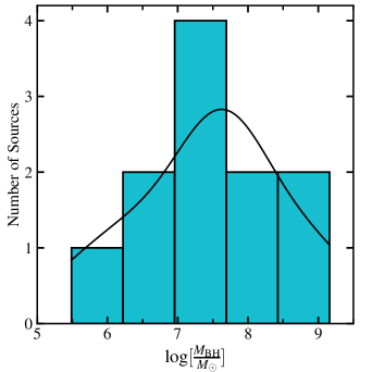
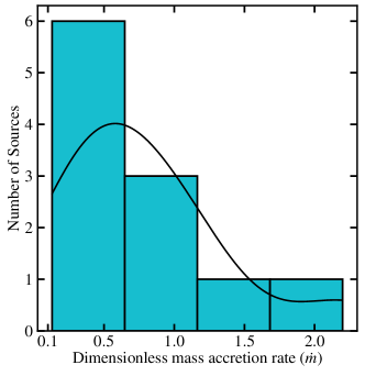
Figure 1: Distribution of black hole mass (left panel) and dimensionless mass accretion rate (right panel) of the AGN sample employed in this work.

2 Sample Selection and Data Processing

We selected the AGN sample from JJ19, who performed high-density disk reflection modeling of 17 AGN using only XMM-Newton data in the energy range of 0.5–10 keV. To better understand the accretion disk/corona coupling and probe the origin of the puzzling soft X-ray excess with the updated high-density disk reflection model as well as test the relevance of additional warm Comptonization, we selected the 11 AGN from the JJ19 sample that do not show absorption in the spectra extracted from the charge-coupled device (CCD) data of XMM-Newton (0.3–10 keV). Additionally, we employed the available NuSTAR (3$-$78 keV) data to probe the hard X-ray excess emission and constrain the broadband primary X-ray continuum in the sample.

The basic characteristics of the selected 11 AGN are presented in Table 1. Two key parameters crucial for this work are the black hole mass and dimensionless mass accretion rate, which are given in columns (4) and (7), respectively. The black hole masses are measured through optical reverberation mapping and obtained from the AGN Black Hole Mass Database (Bentz & Katz 2015). The dimensionless mass accretion rate was estimated using the observed optical luminosity for each source (see JJ19 for details) and not from the bolometric luminosity due to large uncertainties of the bolometric conversion factor (Vasudevan & Fabian, 2007) and radiative efficiency in AGN (Raimundo et al., 2012). Figure 1 shows the distribution of black hole mass, ${\rm log}[M_{{\rm BH}}/M_{\odot}]$, and dimensionless mass accretion rate ($\dot{m}$) of the 11 AGN employed in our work.

For the selected AGN sample, we utilize archival data from both XMM-Newton (0.3$-$10 keV) and NuSTAR (3$-$78 keV) observatories. This will allow us to apply the updated variable density relativistic disk reflection model to the broadband (0.3$-$78 keV) X-ray spectra of the sample for the first time in a systematic way. We will investigate the origin of both the hard and soft X-ray excess emission, testing whether broadband relativistic reflection from a higher-density inner disk is robust enough or an extra warm Comptonization model is still required to model the observed soft X-ray excess of the AGN sample, compute the disk-to-corona power transfer fraction for the first time in any accreting objects, and constrain the SMBH spin population across mass scales utilizing joint XMM-Newton/NuSTAR reflection spectroscopy. The observation details of the sample are presented in Table A1.

2.1 XMM-Newton Data Extraction

We start our work by collecting all the raw data of our sample from the XMM-Newton observatory available in the HEASARC archive. We process the raw data from the European Photon Imaging Camera (EPIC) onboard XMM-Newton in the Scientific Analysis System (SAS v.21.0.0) with the most recent calibration files as of July 2024. First, we generated raw event files from EPIC-pn and MOS data with SAS tasks epproc and emproc, respectively. To exclude the background flares, we created good time intervals (GTI) above 10 keV for the full field using the technique detailed in Mallick et al. (2021). We extracted flare-filtered clean event files by applying the flare-corrected GTI and unflagged events with PATTERN$\leq 4$ for EPIC-pn and PATTERN$\leq 12$ for EPIC-MOS. The EPIC-pn data have much better sensitivity above 6 keV and suffer less from pile-up effects compared to the EPIC-MOS data. Therefore, we concentrate on the EPIC-pn data of the sample. However, we notice that the EPIC-pn events of UGC 6728 are flaring background-dominated. Hence, we consider the EPIC-MOS data only for UGC 6728. The source and background events are extracted from a circular region of radius 35 arcsec centered on the point source and nearby source-free area, respectively. We checked for the presence of pile-up effects using the epatplot task. Whenever pile-up was detected, we removed the central bright pixels by choosing an annular source region. We choose the inner radius of the annulus such that the distributions of the observed data match the model curves produced by epatplot. We generate the redistribution matrix file (rmf) and ancillary response file (arf), source, and background spectra using the SAS task especget. We binned the source spectra including background with the FTOOL task ftgrouppha, where we set grouptype=optsnmin and groupscale=5. The grouptype=optsnmin uses the optimal binning algorithm of Kaastra & Bleeker (2016) with an additional requirement of a minimum signal-to-noise ratio per grouped bin set by groupscale. We fit the XMM-Newton/EPIC spectra in the entire energy range of 0.3$-$10 keV. The EPIC camera, Obs. ID, start time of the observation, total elapsed time, net exposure, net count rate, and net counts in the 0.3$-$10 keV band for each source are listed in Table A1.

2.2 NuSTAR Data Extraction

NuSTAR observed all the sources in our sample with its two co-aligned Focal Plane Modules, A (FPMA) and B (FPMB). We acquired all the available data from the HEASARC archive and reduced the raw (level 1) data in the NuSTAR Data Analysis Software (NuSTARDAS v.2.1.2). We produced the cleaned and calibrated event files with the nupipeline task using the latest (as of 2024 July 24) calibration database (CALDB version: 20240701). We employed conservative criteria, saamode=optimized and tentacle=yes, to treat the high background levels induced by the South Atlantic Anomaly (SAA) region. To maximize the signal-to-noise ratio, we determine the optimal radius of a circular extraction region centered on the source using the NuSTAR tool nustar-gen-utils for each observation. The corresponding background extraction region was selected from the same-sized circular off-source region. We produced the response matrices (rmf and arf), source, and background spectra for both FPMA and FPMB with the nuproducts task. Finally, we generated background-subtracted binned spectra using the ftgrouppha tool, where we employ the optimal binning algorithm of Kaastra & Bleeker (2016) and minimum signal-to-noise ratio of 5 per grouped bin for both FPMA and FPMB. We fit the calibrated energy range of 3$-$78 keV for NuSTAR/FPMA and FPMB spectra. The Obs. ID, observation start time, total elapsed time, net exposure time, net count rate, and net counts in the 3$-$78 keV range for both modules are shown in Table A1.

3 Broadband X-ray Spectroscopy

3.1 Spectral Modeling Procedure

We fit all the XMM-Newton and NuSTAR spectral data together for each source in our sample in the software package XSPEC v.12.13.1 (Arnaud, 1996). We included a constant component (constant) to consider the cross-calibration uncertainties between FPMA and FPMB throughout this work. For simultaneous or quasi-simultaneous XMM-Newton and NuSTAR observations, we multiplied a constant component (constant) to account for the cross-calibration uncertainties between XMM-Newton’s EPIC and NuSTAR’s FPM spectra. The constant component was variable, and all other parameters were tied between simultaneous/quasi-simultaneous EPIC and FPM spectra. In those cases where XMM-Newton and NuSTAR observations were non-simultaneous, we set the photon index of the primary continuum and flux/normalization of each model component to vary between observations. We account for the neutral photoelectric absorption ($N_{\rm H,Gal}$) along the line of sight (LOS) of the source by using the Galactic absorption model TBabs. We set the cosmic elemental abundances of Wilms et al. (2000) and photoionization cross-sections of Verner et al. (1996) in the model TBabs. The Galactic hydrogen column density ($N_{\rm H,Gal}$) accounts for the column density of both the atomic ($N_{\rm{HI}}$) and molecular ($N_{\rm H2}$) hydrogen. The $N_{\rm H,Gal}$ value for each source is obtained from Willingale et al. (2013) (listed in Table 1) and kept fixed throughout the spectral fitting. We apply the Cash statistic ($C$-stat, Cash 1979) to find the best-fit model parameters and the $\chi^{2}$ statistic to test the goodness of fits. Once the best-fit model parameters are found, we run Markov Chain Monte Carlo (MCMC) analyses to determine the parameter uncertainties. The quoted uncertainties on each best-fit parameter represent 90% confidence intervals.

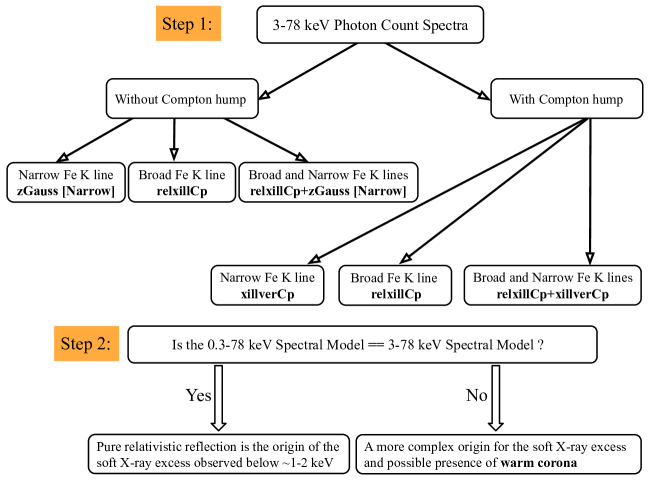
Figure 2: The flowchart depicts our step-by-step spectral fitting methodology, which unambiguously probes the origin of the soft X-ray excess in the sample containing diverse spectral features.

3.2 Basic Spectral Exploration

To unambiguously detect any spectral features, we first consider the continuum bands, 3$-$5 keV and 7$-$10 keV, solely dominated by the primary coronal emission. We fit the 3$-$5 keV and 7$-$10 keV bands by the Galactic absorption corrected power-law model (TBabs$*$zpowerlw). In search of various spectral features, we extrapolate the best-fit primary power-law continuum model over the whole 0.3$-$78 keV energy range. The XMM-Newton EPIC-pn (MOS for UGC 6728) and NuSTAR FPMA/B spectral data, the Galactic absorption corrected power-law continuum model, and data-to-model ratio plots for the sample are shown in Fig. A1. The ratio plots reveal a soft X-ray excess below $\sim 1-2$  keV and Fe K emission in the $\sim 6-7$  keV band for all AGN. We detected a prominent Compton hump in the range of $\sim 15-30$  keV for most sources in our sample.

3.3 Probing the Hard X-ray Excess Emission: 3$-$78 keV Spectral Modeling

As evident from Fig. A1, the X-ray photon count spectra of the sample are complex, with an excess emission in the soft X-ray band. Therefore, we start our spectral modeling first considering the hard X-ray (3$-$78 keV) photon count spectra and probe the Fe K emission as well as the Compton hump. We describe the hard X-ray primary continuum by the physically motivated nthComp model (Zdziarski et al., 1996), which produces a power-law like continuum due to the thermal Comptonization of disk seed photons in a hot corona of electrons. The free parameters of the nthComp model are photon index ($\Gamma$), electron temperature ($kT_{\rm e}$), and normalization.

In the 6$-$7 keV band, we can obtain either narrow or broad or both narrow and broad Fe K emission features. However, the narrow Fe K emission features are never resolved in low-resolution CCD data. Therefore, while performing progressive spectral fitting to assess the presence of Fe emission from the torus or other distant material, we first add a simple Gaussian line zGauss[Narrow] with its width fixed at $10$ eV (see e.g. Mallick et al. 2017), which is smaller than the resolution of EPIC-pn at $\sim 6-7$  keV or utilize a distant reflection model to fit the narrow Fe K emission features. Any additional contribution to the line profile would then come from material closer to the black hole, which is characterized by relativistic disk reflection.

We notice that the Compton hump is either very weak or undetected for some AGN in the sample. When the Compton hump is not detected, and the Fe K band contains only a narrow emission feature at $\sim 6.4$ keV, we use the simple narrow Gaussian line zGauss[Narrow]. In this case, we can write the best-fit hard X-ray spectral model of the source as nthcomp$+$zGauss[Narrow]. The broad emission feature in the Fe K band is characteristic of relativistic reflection from the inner accretion disk (Fabian et al., 1989, 2002). Therefore, we apply the relativistic disk reflection model relxillCp (García et al., 2016, 2014; Dauser et al., 2014) to fit the detected broad Fe K emission. We set refl$\_$frac$=-1$ in the relxillCp model to fit only the reprocessed emission from the accretion disk. The parameters (photon index $\Gamma$ and electron temperature $kT_{\rm e}$) that describe the properties of the corona are tied between relxillCp and nthComp models. The relxillCp table model is calculated with the seed photon temperature of the accretion disk fixed at 50 eV. Accordingly, we set the input disk seed photon temperature at 50 eV in the nthComp model for consistency. The relevant input parameters of the relxillCp model are:

• Electron density ($n_{\rm e}$) of the accretion disk.

• Iron abundance ($A_{\rm Fe}$) in the disk relative to solar.

• The dimensionless spin ($a^{\ast}$) of the black hole, which is measured by setting the inner radius ($r_{\rm in}$) of the accretion disk at the innermost stable circular orbit ($r_{\rm isco}$). To meet the criterion, we need to set Rin=-1 in the model.

• Inclination angle ($\theta^{\circ}$) of the disk relative to the line of sight.

• Disk ionization parameter, $\xi=\frac{4\pi F}{n_{\rm e}}$, where $F$ is the illuminating continuum flux.

• The emissivity profile of the accretion disk, which is a measure of the reflected flux as a function of disk radius and is parameterized by a broken power law: $\epsilon(r)\propto r^{-q_{\rm in}}$ for $r_{\rm in}\leq r\leq r_{\rm br}$, and $\epsilon(r)\propto r^{-q_{\rm out}}$ for $r_{\rm br}\leq r\leq r_{{\rm{\rm out}}}$. The inner emissivity index ($q_{\rm in}$) is a free parameter in the model. Over the outer disk, the emissivity profile falls as $r^{-3}$, as expected in flat spacetime. Therefore, we fix the outer emissivity index at $q_{\rm out}=3$. The break radius corresponds to the radial extent of the corona and is fixed at $r_{\rm br}=6r_{\rm g}$, a typical value for the coronal radius in AGN (Mallick et al., 2021, 2022).

In the absence of a prominent Compton hump, when the Fe K band reveals both the narrow 6.4 keV line emission and relativistically broad emission feature, we find that the model, relxillCp$+$zGauss[Narrow]$+$nthcomp, describes the hard X-ray spectra the best. A flowchart of our spectral fitting methodology is demonstrated in Figure 2. When the Compton hump is detected, we employ the non-relativistic reflection model (xillverCp, García et al. 2013) to fit the narrow Fe K emission line(s) together with the Compton hump. Within xillverCp, we set refl$\_$frac$=-1$ and tied the coronal parameters (photon index $\Gamma$ and electron temperature $kT_{\rm e}$) to those in nthComp. The density of the reflector in the distant reflection model (xillverCp) is kept fixed at the canonical value of $n_{\rm e}=10^{15}~\rm{cm}^{-3}$ throughout the spectral fitting. The distant reflector is assumed to be near-neutral ($\log\xi=0$) and has a high inclination angle of $\theta=60^{\circ}$ (e.g. Mallick et al. 2018; Zhao et al. 2021). When both the broad Fe K emission line and Compton hump are detected, the hard X-ray (3$-$78 keV) spectra are best described by either model relxillCp$+$nthcomp or relxillCp$+$xillverCp$+$nthcomp, where the relativistic disk reflection (relxillCp) models the broad Fe K line, and the Compton hump is fitted by either relativistic disk reflection (relxillCp) or by a combination of both relativistic (relxillCp) and distant (xillverCp) reflection models. We link the coronal parameters of the nthComp model with those in relxillCp and xillverCp. The iron abundance ($A_{\rm Fe}$) in the disk was tied between relxillCp and xillverCp. When the Compton hump is detected, and the Fe K band contains both the narrow and broad emission lines, the model that best explains the hard X-ray spectral data is relxillCp$+$xillverCp$+$nthcomp. Figure 2 (Step 1) illustrates our methods of fitting various spectral features in the hard X-ray (3$-$78 keV) photon count spectra.

3.4 Probing Both Soft and Hard X-ray Excess: 0.3$-$78 keV Spectral Modeling

Once the hard X-ray best-fit spectral models have been found for the sample, we extrapolate that model down to 0.3 keV, to see whether the same model can fit the whole 0.3$-$78 keV spectra or not. When the hard X-ray best-fit spectral model of an AGN can also explain the soft X-ray excess emission without the need for any extra blackbody or low-temperature Comptonization model, it will justify that the same physical mechanism is responsible for the origin of the soft X-ray excess emission, i.e., the relativistic reflection from an accretion disk with variable density. If the hard X-ray spectral model cannot fully describe the soft X-ray band and a warm Comptonization model is indeed needed, we can conclude that the origin of the observed soft X-ray excess is the relativistic disk reflection together with a warm coronal emission. We present our methodology of fitting the hard-to-soft X-ray excess emission as a flowchart in Fig. 2 (Step 2). The 0.3$-$78 keV joint XMM-Newton/NuSTAR spectral modeling of the sample shows that higher-density relativistic disk reflection can simultaneously fit the soft X-ray excess, broad Fe K emission line, and Compton hump for 8 out of 11 AGN in our sample. For the remaining 3 AGN, an additional warm Comtonization model (compTT) is still required to fit the soft X-ray excess. Fig. A2 shows the XMM-Newton/EPIC, NuSTAR/FPMA, and FPMB photon count spectra, the best-fit count spectral models of the sample along with the model components. We present the best-fit flux spectral model with components in Fig. A3. The best-fit broadband (0.3$-$78 keV) spectral model parameters for each source are presented in Table A2. In Appendix A, we discuss the hard-to-soft X-ray spectral fitting details for each source in the sample.

3.5 Relative contributions of relativistic and distant reflection in the Fe K band

We characterize the relative contributions of the relativistic and distant reflection components in the $5-7$ keV Fe K band to comprehend their respective strengths. Figure 3 demonstrates the relativistic disk reflected flux vs. the non-relativistic or distant reflection flux relative to the primary continuum flux in the Fe K band. The 1:1 line denotes the equal relative contributions of the relativistic and distant reflection to the continuum, i.e.,

$$\left(\frac{F_{\rm relativistic~reflection}}{F_{\rm primary~continnum}}\right)_{[5-7{\rm~keV}]}=\left(\frac{F_{\rm distant~reflection}}{F_{\rm primary~continnum}}\right)_{[5-7{\rm~keV}]}.$$

From Fig. 3, we can see that relativistic reflection contributes more than the distant reflection in the Fe K band for all sources in the diagram except for Mrk 79 and some observations of Mrk 279, possibly because these two sources show both Fe K_α and Fe K_β emission lines. Additionally, we notice the variable nature of the relativistic disk reflected flux responsible for the broad Fe K emission whenever we have multiple flux measurements of a source. However, as expected, the distant reflection flux characterizing the narrow Fe K emission line(s) appears non-variable or constant within error bars.

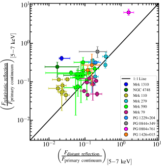
Figure 3: The flux of the relativistic reflection (relxillCp) model versus non-relativistic or distant reflection (either zGauss[Narrow] or xillverCp) model relative to the primary continuum (nthComp) flux in the $5-7$ keV band, demonstrating the relative contributions of the relativistic and distant reflection components in the Fe K band. The $1:1$ line represents $\left(\frac{F_{\rm relativistic~reflection}}{F_{\rm primary~continnum}}\right)_{[5-7{\rm~keV}]}=\left(\frac{F_{\rm distant~reflection}}{F_{\rm primary~continnum}}\right)_{[5-7{\rm~keV}]}$. We included observations with constrained flux values.

Table 2: Details of the Bayesian statistical test performed to examine the significance of a higher-density (variable $\log n_{e}$) accretion disk over the canonical ($n_{\rm e}=10^{15}$ cm^-3) disk reflection model and the relevance of an extra warm Comptonization for soft X-ray excess against the higher-density disk reflection model. Columns (2) and (3) show the Deviance Information Criteria, ${\rm DIC}_{1}$ and ${\rm DIC}_{2}$, for the fixed low-density and variable higher-density disk reflection models, respectively. Column (4) shows the difference between ${\rm DIC}_{1}$ and ${\rm DIC}_{2}$. Column (5) shows the relevance of higher-density against the canonical disk. Column (6) shows the Deviance Information Criterion, ${\rm DIC}_{3}$, for the higher-density disk reflection plus the warm Comptonization model. Columns (7) and (8) report the difference between ${\rm DIC}_{2}$ and ${\rm DIC}_{3}$, and the relevance of an extra warm Comptonization for the origin of soft X-ray excess against the higher-density disk reflection model.

Source	${\rm DIC}_{\rm 1}$	${\rm DIC}_{\rm 2}$	$\Delta{\rm DIC_{12}}$	Evidence of higher-density disk	${\rm DIC}_{\rm 3}$	$\Delta{\rm DIC_{23}}$	Relevance of additional
			${\rm DIC}_{\rm 1}-{\rm DIC}_{\rm 2}$	against canonical low-density		${\rm DIC}_{\rm 2}-{\rm DIC}_{\rm 3}$	warm corona over the
							higher-density disk
(1)	(2)	(3)	(4)	(5)	(6)	(7)	(8)
UGC 6728	$543.4$	$543.9$	$-0.5$	Negative [$\Delta{\rm DIC}<0$]	$545.2$	$-1.3$	Negative [$\Delta{\rm DIC}<0$]
Mrk 1310	$299.4$	$299.2$	$0.2$	Neutral [$\Delta{\rm DIC}<2$]	$311.5$	$-12.3$	Negative [$\Delta{\rm DIC}<0$]
NGC 4748	$329.3$	$306.7$	$22.6$	Very Strong [$\Delta{\rm DIC}>10$]	$290.6$	$16.1$	Very Strong [$\Delta{\rm DIC}>10$]
Mrk 110	$2125.8$	$1995.2$	$130.6$	Very Strong [$\Delta{\rm DIC}>10$]	$1861.4$	$133.8$	Very Strong [$\Delta{\rm DIC}>10$]
Mrk 279	$1473.6$	$1463.2$	$10.4$	Very Strong [$\Delta{\rm DIC}>10$]	$1507.5$	$-44.3$	Negative [$\Delta{\rm DIC}<0$]
Mrk 590	$2328.0$	$2319.3$	$8.7$	Strong [$\Delta{\rm DIC}=6-10$]	$2341.0$	$-21.7$	Negative [$\Delta{\rm DIC}<0$]
Mrk 79	$1706.8$	$1211.0$	$495.8$	Very Strong [$\Delta{\rm DIC}>10$]	$1296.0$	$-85.0$	Negative [$\Delta{\rm DIC}<0$]
PG 1229+204	$191.1$	$184.7$	$6.4$	Strong [$\Delta{\rm DIC}=6-10$]	$193.0$	$-8.3$	Negative [$\Delta{\rm DIC}<0$]
PG 0844+349	$228.4$	$225.1$	$3.3$	Positive [$\Delta{\rm DIC}=2-6$]	$234.5$	$-9.4$	Negative [$\Delta{\rm DIC}<0$]
PG 0804+761	$371.6$	$295.6$	$76.0$	Very Strong [$\Delta{\rm DIC}>10$]	$298.5$	$-2.9$	Negative [$\Delta{\rm DIC}<0$]
PG 1426+015	$669.1$	$575.8$	$93.3$	Very Strong [$\Delta{\rm DIC}>10$]	$534.6$	$41.2$	Very Strong [$\Delta{\rm DIC}>10$]

3.6 MCMC Analysis for Parameter Space Exploration

To confirm that the parameters are not clustering at any local minima, we conduct an MCMC analysis on the best-fit model and explore the complete parameter space for each source. We draw the parameter distributions and determine confidence intervals for each free parameter from the converged MCMC chains. To run the MCMC chains, we use the algorithm of Goodman & Weare (2010) implemented in XSPEC. We run MCMC chains with 100-300 walkers for $\sim 10^{6}-10^{7}$ iterations and burn the first $\sim[1-10]$% iterations until the chains were converged. We notice the number of walkers needed to be at least four times greater than the number of free parameters in the model for faster convergence of chains. We ensured that the chains converged with Gelman–Rubin’s MCMC convergence test, which resulted in the potential scale reduction factor being less than 1.1 for each parameter. The full posterior distributions of various model parameters and contour plots between each pair of parameters for all sources in the sample are shown in Figures A4 and A5. The dark, medium, and light blue contours represent 68.3%, 90%, and 95% confidence levels, respectively.

3.7 Bayesian Analysis for Model Selection

First, we test the relevance of the high-density disk (variable $\log n_{e}$) over the canonical ($\log[n_{\rm e}/\rm{cm}^{-3}]=15$) disk reflection model by fixing the density parameter in the best-fit spectral model at the canonical value of $n_{\rm e}=10^{15}$ cm^-3 and refit all the spectra for each source, which resulted in higher fit statistics. However, comparing only the fit statistics between two models is inconclusive because one model might over-fit the data for having more free parameters or under-fit the data, resulting in a higher $\chi^{2}$-statistic. Therefore, we implement a Bayesian model selection approach, where the posterior distributions of the models are computed from MCMC simulations. We employ the Deviance Information Criterion, DIC (Spiegelhalter et al., 2002), which is a Bayesian model selection metric and defined by

$${\rm DIC}=\overline{D(\theta)}+p_{D},$$

where $D(\theta)=-2\log\left(p(y|\theta)\right)$ and $p_{D}=\overline{D(\theta)}-D(\bar{\theta})$. Here $p(y|\theta)$ is the likelihood function, $D(\theta)$ is the deviance of a model parameter $\theta$, $y$ represent the data and $p_{D}$ is the effective number of parameters in the model.

DIC considers both the goodness of fit evaluated by the likelihood function and an effective number of model parameters. DIC is a hierarchical modeling generalization of the Akaike information criterion, AIC (Akaike, 1974). However, DIC does not penalize a model for parameters unconstrained by the data (Kass & Raftery, 1995) because it uses an effective number of parameters, unlike AIC. DIC considers a model parameter only if it affects the goodness of fit to the data and is altered by varying that parameter. The degree to which different parameters are constrained is reflected in the non-integer nature of the effective number of model parameters.

In order to confirm whether a higher-density disk is preferred over the canonical disk reflection model, we compare the DIC calculated from these two models. Statistically, the model with a lower DIC is preferred by the data, and the difference in DIC, $\Delta{\rm DIC}$, between the two models measures the strength of the preference. According to a scale proposed by Jeffreys (1961) and updated by Kass & Raftery (1995), the $\Delta{\rm DIC}$ values between 0 and 2 hint only marginal evidence, $\Delta{\rm DIC}$ between 2 and 6 provides positive evidence, $\Delta{\rm DIC}$ between 6 and 10 suggests strong evidence, and $\Delta{\rm DIC}$ greater than 10 shows very strong evidence for one model over another. In Table 2, columns (2), (3), (4), and (5), respectively, show the ${\rm DIC}_{\rm 1}$ and ${\rm DIC}_{\rm 2}$ computed from fixed low-density and variable higher-density disk reflection models, their difference $\Delta{\rm DIC_{12}}={\rm DIC}_{\rm 1}-{\rm DIC}_{\rm 2}$ and the DIC scale determining the evidence of the higher-density disk against the canonical disk reflection model. As a next step, to test the significance of warm coronal emission for the origin of soft X-ray excess, we add warm Comptonization to the high-density disk reflection model, refit all the spectra, and evaluate DIC for the higher-density disk reflection plus the warm Comptonization model for each source, which is denoted as ${\rm DIC}_{\rm 3}$ in column (6) of Table 2. The difference between DICs without and with warm Comptonization is presented as $\Delta{\rm DIC_{23}}={\rm DIC}_{\rm 2}-{\rm DIC}_{\rm 3}$ in column (7) of Table 2. The DIC scale in column (8) of Table 2 indicates the significance of additional warm Comptonization over the high-density disk reflection model for the origin of the observed soft X-ray excess.

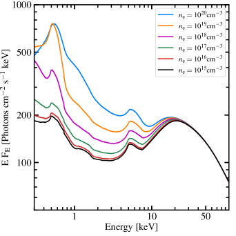
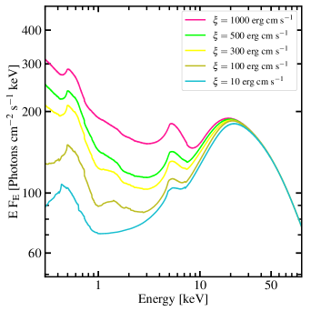
Figure 4: The left panel shows the spectra calculated by the relativistic reflection model, relxillCp, for a range of disk densities, $\log[n_{\rm e}/\rm{cm}^{-3}]=15$, $16$, $17$, $18$, $19$, and $20$. The standard model parameters are assumed to be $\Gamma=2$, $kT_{\rm e}=300$ keV, $\xi=500$ erg cm s^-1, $q_{\rm in}=8$, $a^{\ast}=0.9$, $\theta=45^{\circ}$, and $A_{\rm Fe}=1$. We can see a significant boost in the strength of the soft X-ray component from the disk density of $n_{\rm e}=10^{17}\rm{cm}^{-3}$ onward. The right panel depicts the spectra for various ionization states ($\xi/{\rm erg~cm~s^{-1}}=10$, $100$, $300$, $500$, and $1000$) of the accretion disk in the relxillCp model calculated for $\Gamma=2$, $kT_{\rm e}=300$ keV, $\log[n_{\rm e}/\rm{cm}^{-3}]=17$, $q_{\rm in}=8$, $a^{\ast}=0.9$, $\theta=45^{\circ}$, and $A_{\rm Fe}=1$. Even for the same disk density, the soft X-ray excess flux is enhanced with a broader Fe K line as the disk becomes more ionized upto $\log[\xi/$erg cm s${}^{-1}]=3$.

4 Results and Discussion

In this section, we discuss all the results derived from our broadband X-ray spectral modeling, the implications of the physical reflection model for the origin of the soft X-ray excess, the validity of the standard SS73 accretion disk theory, the first-time calculation of the disk-to-corona power transfer fraction, coronal properties, and black hole spin population across mass scales ($\log M_{\rm BH}\sim 5.5-9.0$). The details of broadband spectral modeling for each source in the sample are presented in Appendix A. In Table A2, we report the best-fit source spectral model parameters and their 90% confidence intervals determined through MCMC parameter space exploration of the best-fit model. Fig. A2 shows the broadband XMM-Newton/NuSTAR spectra, the best-fit count spectral model with components, and the corresponding residuals. The best-fit spectral energy flux models with components are presented in Fig. A3.

4.1 Physical Origin of the Soft X-ray Excess Emission: High-density disk reflection or warm Comptonization

Two models have been proposed to explain the observed soft X-ray excess. One model is the relativistic reflection or reprocessing of the incident hot coronal emission in the innermost part of the accretion disk (George & Fabian, 1991; Ross & Fabian, 2005; García et al., 2014). The other model considers Compton up-scattering of the optical/UV disk photons in a low-temperature ($kT\sim 0.1-2$ keV), optically thick ($\tau>1$) Comptonzing medium or warm corona (Done et al., 2012; Petrucci et al., 2018). However, the relativistic reflection as the origin of the soft X-ray excess is a more consistent explanation since it is the only model that can explain the broad Fe K line and Compton hump together with the soft X-ray excess. However, it was shown that the entire soft X-ray excess may not be well-fitted solely by relativistic reflection (e.g. Ark 120: Mallick et al. 2017; Porquet et al. 2018), especially when the disk density is low and fixed at $\log[n_{\rm e}/\rm{cm}^{-3}]=15$. Furthermore, fitting of soft X-ray excess with a fixed low-density relativistic disk reflection model resulted in unphysically high ($A_{\rm Fe}>10$) iron abundance in some sources (e.g. 1H 0707-495: Dauser et al. 2012). To resolve these issues, García et al. (2016) developed a new model where the density of the accretion disk is a free parameter varying in the range of $\log[n_{\rm e}/\rm{cm}^{-3}]=15-20$, first implemented by Mallick et al. (2022). When the innermost part of the disk becomes radiation-pressured dominated, extra heating produced by the free-free emission increases the disk density, thus boosting the strength of the observed soft X-ray excess below 1 keV (Ross & Fabian, 2007; García et al., 2016). In Fig. 4 (left), we show the flux spectra calculated from the variable density disk reflection model relxillCp for the disk density of $\log[n_{\rm e}/\rm{cm}^{-3}]=15$, $16$, $17$, $18$, $19$, and $20$. The standard parameters assumed for the model calculations are $\Gamma=2$, $kT_{\rm e}=300$ keV, $\xi=500$ erg cm s^-1, $q_{\rm in}=8$, $a^{\ast}=0.9$, $\theta=45^{\circ}$, and $A_{\rm Fe}=1$. Even with the solar iron abundance, model flux is noticeably enhanced at the soft X-ray band when the disk density is higher than $n_{\rm e}=10^{15}\rm{cm}^{-3}$, and the difference from the canonical disk reflection model becomes more prominent for $n_{\rm e}\geq 10^{17}\rm{cm}^{-3}$.

Disk ionization is also an important physical parameter in the relativistic disk reflection model (relxillCp) and affects the strength of the observed soft X-ray excess. To illustrate how it affects the spectral components, especially the soft X-ray excess and broad Fe K line, we show the flux spectra for the disk ionization of $\xi/{\rm erg~cm~s^{-1}}=10$, $100$, $300$, $500$, and $1000$ in the right panel of Fig. 4. The other standard parameters considered for the model calculations are $\Gamma=2$, $kT_{\rm e}=300$ keV, $\log[n_{\rm e}/\rm{cm}^{-3}]=17$, $q_{\rm in}=8$, $a^{\ast}=0.9$, $\theta=45^{\circ}$, and $A_{\rm Fe}=1$. Evidently, as the disk becomes more ionized, the soft X-ray flux is enhanced with a broader Fe K line, even for the same electron density of the accretion disk.

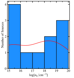
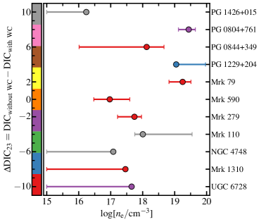
Figure 5: The left panel shows the distribution of the measured electron density of the accretion disk for our sample. The colorbar in the right panel depicts the difference between the Deviance Information Criteria, ${\rm DIC}_{{\rm without~WC}}$ and ${\rm DIC}_{{\rm with~WC}}$, for the variable density disk reflection model without and with warm Comptonization, respectively. The Bayesian model selection metric supports the relevance of additional warm Comptonization for the origin of soft X-ray excess in 3 AGN (Mrk 110, NGC 4748, and PG 1426$+$015), marked in grey color.

The distribution of the disk density parameter for the sample is shown in Fig. 5 (left panel). Through Bayesian analysis, we find positive-to-very strong evidence for variable higher-density disk against the canonical one with $\Delta{\rm DIC_{12}}$ ranging from 2 to above 10, as shown in columns (2)–(5) of Table 2. We obtained disk density measurements higher than the canonical value of $\log[n_{\rm e}/{\rm cm^{-3}]}=15$ with 90% confidence for all sources except four: UGC 6728, Mrk 1310, NGC 4748 and PG 1426$+$015. Out of these four AGN, UGC 6728 and Mrk 1310 did not show strong relativistic reflection features in the X-ray spectra. The other two AGN, NGC 4748 and PG 1426$+$015, exhibited strong relativistic reflection features (broad Fe K line, Compton hump) yet required a warm Comptonization component for soft X-ray excess in addition to the variable density relativistic disk reflection where the 90% lower limit of the density parameter reached $\log[n_{{\rm e}}/{\rm cm^{-3}]}=15$. However, we notice that for one AGN, i.e., Mrk 110, both the high-density relativistic disk reflection with well-constrained $\log[n_{{\rm e}}/{\rm cm^{-3}]}=18.0_{-0.3}^{+1.5}$ and warm Comptonization are required to explain its broadband spectral emission comprehensively. The right panel in Fig. 5 shows $\Delta{\rm DIC_{23}}$ versus disk density for the sample, confirming the relevance of the warm coronal emission for the origin of the observed soft X-ray excess in 3 (NGC 4748, Mrk 110, and PG 1426$+$015) out of 11 AGN. The temperature and optical depth of the warm corona for these 3 AGN are found to be in the range of $kT_{\rm wc}\sim 0.25-2$ keV and $\tau_{\rm wc}\sim 4-17$, respectively, which agree with the properties of the warm corona constrained from a sample of AGN (see Fig. 5 of Petrucci et al. 2018). Through joint XMM-Newton+NuSTAR broadband spectroscopy, we find that the high-density relativistic reflection can self-consistently explain both the broad Fe K line and soft X-ray excess in 8 out of 11 AGN. The inner accretion disk is found to be ionized and dense, with the median ionization of $\xi\sim 10^{2.5}$ erg cm s^-1, median density of $n_{\rm e}\sim 10^{17.8}\rm{cm}^{-3}$, and near-solar iron abundance of $A_{\rm Fe}\sim 2$ for the sample.

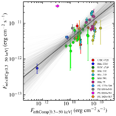
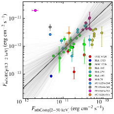
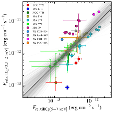
Figure 6: The left panel shows the variation in relativistic disk reflected flux with the directly observed continuum flux in the 0.3–50 keV range. The solid black line depicts the best-fit model and has the form $F_{\rm relxillCp[0.3-50~keV]}\propto F_{\rm nthComp[0.3-50~keV]}^{0.63\pm 0.15}$. The variation in relativistic disk reflected flux in the soft X-ray excess dominated 0.3–2 keV band as a function of the directly observed continuum flux in the 2–50 keV band is presented in the middle panel, where the solid black line shows the best-fit model and follows the form $F_{\rm relxillCp[0.3-2~keV]}\propto F_{\rm nthComp[2-50~keV]}^{1.4\pm 0.6}$. Both these plots demonstrate a positive correlation between relativistic disk reflection and primary continuum flux in the soft (0.3–2 keV), hard (2–50 keV), and broad (0.3–50 keV) energy bands. The right panel shows the variation in relativistic disk reflected flux in the soft X-ray excess dominated 0.3–2 keV band versus the broad Fe K line dominated 5–7 keV band. The best-fit model shown in the solid black line has the form $F_{\rm relxillCp[0.3-2~keV]}\propto F_{\rm relxillCp[5-7~keV]}^{1.2\pm 0.2}$, suggesting correlated variability between the broad Fe K line and soft X-ray excess emission, which is expected if they both have relativistic disk reflection origin. In all these three plots, we included observations for which both X and Y values are constrained.

4.2 Energy-dependent Correlated Variability of Reflected and Direct Continuum Flux

In this section, we explore the variations of relativistic disk reflection and direct continuum in different energy bands and their interconnection for the sample. First, we probe the dependence of relativistic disk reflection on the direct continuum in the broad 0.3–50 keV range since this energy range includes all three relativistic reflection features: soft X-ray excess, broad Fe K line, and Compton hump. The left panel in Figure 6 shows the variation in relativistic disk reflected flux $\left(F_{\rm relxillCp[0.3-50~keV]}\right)$ as a function of the directly observed continuum flux $\left(F_{\rm nthComp[0.3-50~keV]}\right)$ in the 0.3–50 keV energy range of the sample. We assess the correlation between relativistic disk reflection and primary continuum by performing a Spearman’s rank correlation test on the sample and find a positive correlation between $F_{\rm relxillCp[0.3-50~keV]}$ and $F_{\rm nthComp[0.3-50~keV]}$ with a Spearman correlation coefficient of $\rho_{s}=0.52$ and a null hypothesis (p-value) probability of $9.4\times 10^{-5}$. Though the degree of correlation is moderate due to an outlier (Fig. 6, left), the significance of the observed correlation is high, as indicated by the p-value. If we discard the outlier, we obtain an even stronger correlation with the Spearman correlation coefficient of $\rho_{\rm s}=0.61$ and a p-value of $2.9\times 10^{-6}$. We also perform a Bayesian linear regression analysis, which considers errors in both independent and dependent variables (Kelly, 2007). The best-fit $\log F_{\rm relxillCp[0.3-50~keV]}$ versus $\log F_{\rm nthComp[0.3-50~keV]}$ Bayesian regression model for the sample is

$$\log F_{{\rm relxillCp[0.3-50~keV]}}=\log F_{{\rm nthComp[0.3-50~keV]}}^{0.63\pm 0.15}-(4.5\pm 1.6).$$

The black solid line and grey shaded area in the left panel of Fig. 6, respectively, show the best-fit model and corresponding $1\sigma$ confidence interval. The best-fit model $F_{\rm relxillCp[0.3-50~keV]}\propto F_{\rm nthComp[0.3-50~keV]}^{0.63\pm 0.15}$ suggests a correlated variability between the disk reflected and directly observed continuum flux, which is in agreement with the relativistic reflection scenario (Wilkins et al. 2014; Mallick & Dewangan 2018). When the primary X-ray source or corona is close to the black hole, strong light bending causes a greater fraction of the rays from the corona to be focused onto the inner regions of the accretion disk, producing the relativistic disk reflected emission. Therefore, if the intrinsic luminosity of the source remains constant, the reflected flux will increase as the primary continuum flux increases (see Wilkins et al. 2014).

In the relativistic disk reflection scenario, if the observed soft X-ray excess is produced due to irradiation of the inner accretion disk by the primary X-ray source, we expect a correlated variability between soft X-ray excess and direct continuum. Hence, we explore the variation in the relativistic disk reflected flux $\left(F_{\rm relxillCp[0.3-2~keV]}\right)$ in the 0.3–2 keV band as a function of the directly observed continuum flux $\left(F_{\rm nthComp[2-50~keV]}\right)$ in the 2–50 keV for the sample (Fig. 6, middle), where the 0.3–2 keV and 2–50 keV energy bands are mainly dominated by soft X-ray excess and primary X-ray source emission, respectively. We measure the correlation between $F_{\rm relxillCp[0.3-2~keV]}$ and $F_{\rm nthComp[2-50~keV]}$ for the sample, which provided a Spearman correlation coefficient of $\rho_{s}=0.47$ and a null hypothesis (p-value) probability of $6\times 10^{-4}$, implying a moderate positive correlation with high significance. After discarding the one outlier (marked in magenta color), we obtain a more significant and stronger correlation between $F_{\rm relxillCp[0.3-2~keV]}$ and $F_{\rm nthComp[2-50~keV]}$ with $\rho_{s}=0.56$ and p-value $=3\times 10^{-5}$. The best-fit Bayesian linear regression model representing the $\log F_{{\rm relxillCp[0.3-2~keV]}}$ versus $\log F_{{\rm nthComp[2-50~keV]}}$ relation of the sample is

$$\log F_{{\rm relxillCp[0.3-2~keV]}}=\log F_{{\rm nthComp[2-50~keV]}}^{1.4\pm 0.6}+(3.2\pm 6.2),$$

where the best-fit model and associated $1\sigma$ confidence interval are shown by the black solid line and grey shaded area in the middle panel of Fig. 6. The best-fit relation $F_{\rm relxillCp[0.3-2~keV]}\propto F_{\rm nthComp[2-50~keV]}^{1.4\pm 0.6}$ shows that soft X-ray excess flux varies with the directly observed continuum flux, which conforms with the relativistic reflection scenario where the soft X-ray excess results from the extreme relativistic blurring of the reflected emission from the inner regions of the accretion disk.

It is the same relativistic reflection that produces both the broad Fe K line and soft X-ray excess. Therefore, we expect correlated variability between relativistic disk reflected flux in the broad Fe K line dominated 5–7 keV band and that in the soft X-ray excess dominated 0.3–2 keV band. The right panel in Fig. 6 shows the variation in $\log F_{\rm relxillCp[0.3-2~keV]}$ as a function of $\log F_{\rm relxillCp[5-7~keV]}$. The measured Spearman correlation coefficient between $\log F_{\rm relxillCp[0.3-2~keV]}$ and $\log F_{\rm relxillCp[5-7~keV]}$ for the sample is $\rho_{s}=0.71$ with a null hypothesis (p-value) probability of $4.8\times 10^{-9}$, which corroborates a strong positive correlation between these two variables. The best-fit $\log F_{\rm relxillCp[0.3-2~keV]}$ versus $\log F_{\rm relxillCp[5-7~keV]}$ relation as obtained from the Bayesian linear regression analysis of the sample is

$$\log F_{{\rm relxillCp[0.3-2~keV]}}=\log F_{{\rm relxillCp[5-7~keV]}}^{1.2\pm 0.2}+(3.1\pm 2.7).$$

In Fig. 6 (right), we show the best-fit model and corresponding $1\sigma$ confidence interval by the black solid line and grey shaded region, respectively. The best-fit relation $F_{\rm relxillCp[0.3-2~keV]}\propto F_{\rm relxillCp[5-7~keV]}^{1.2\pm 0.2}$ confirms that both soft X-ray excess and broad Fe K line emission vary in a correlated manner. This is possible if the relativistic reflection producing the broad Fe K line is responsible for the soft X-ray excess or contributes significantly to this excess emission.

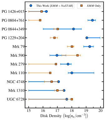
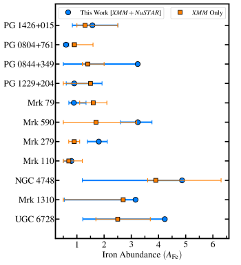
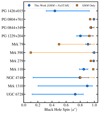
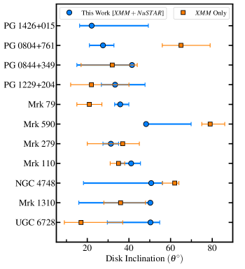
Figure 7: Comparison of disk density, iron abundance, black hole spin, and disk inclination angle obtained from our broadband (0.3–78 keV) joint XMM-Newton+NuSTAR spectral modeling and the previous 0.5–10 keV XMM-Newton spectral fitting of the sample by JJ19. For UGC 6728, Mrk 1310, and PG 1426$+$015, JJ19 fixed the spin parameter at $a^{\ast}=0.998$. Therefore, we cannot compare their spin measurements, and orange squares are absent for these three sources in the bottom left panel. Similarly, no comparison of disk inclination angle is made for PG 1426$+$015 in the bottom right panel since it was a fixed parameter in JJ19.

4.3 Comparison with Previous Study of the Sample with XMM-Newton Only

The comparison of four key parameters, i.e., disk density, iron abundance, black hole spin, and disk inclination angle of the AGN sample obtained from our broadband joint XMM-Newton+NuSTAR spectral modeling and previous analyses using only XMM-Newton data, are presented in Fig. 7. As evident from the top left panel in Fig. 7, the disk density we measured using joint XMM-Newton/NuSTAR data is higher than the one derived from the XMM-Newton spectral fitting alone. This is because the additional spectral features across the broad bandpass let us more accurately disentangle the reflection from the continuum. Moreover, some sources (e.g., Mrk 79) in the previous XMM-Newton data did not show broad Fe K line emission due to short exposure. In this work, with more data from both XMM-Newton and NuSTAR, we prominently detected the broad Fe K emission feature, the modeling of which resulted in an enhanced contribution of the disk reflection component.

The iron abundances measured through our joint XMM-Newton+NuSTAR high-density reflection spectroscopy are consistent with those derived from the high-density reflection modeling of the previous XMM-Newton data of the sample (Fig. 7, top middle). We measure solar or near-solar iron abundance for the sample with a median of $A_{\rm Fe}\sim 2$, which is expected since the higher-density reflection model can decrease the inferred iron abundance by increasing the continuum in the reflection component.

The comparison of the black hole spin parameter with that inferred from the previous high-density spectral fitting of only XMM-Newton data provides consistent results within 90% confidence limits (Fig. 7, bottom middle). Previously, JJ19 fixed the spin parameter at $a^{\ast}=0.998$ while performing the XMM-Newton spectral modeling for three sources (UGC 6728, Mrk 1310, and PG 1426$+$015) due to the non-detection of the broad Fe K line in the XMM-Newton data or unavailability of the hard X-ray data above 10 keV. In this work, the inclusion of the NuSTAR data and hence reflection Compton hump constraints the continuum emission better, which can potentially impact the determination of the red wing of the broad Fe K line and thus affect the black hole spin measurements. As a result, our broadband spectroscopy increases both the accuracy and precision of the black hole spin for all sources in the sample. Moreover, through the joint XMM-Newton/NuSTAR high-density relativistic reflection spectroscopy, we provide the first measurements of black hole spin for three AGN: UGC 6728, Mrk 1310, and PG 1426$+$015.

Previous measurements of the disk inclination angle only using XMM-Newton data provided extreme values that were either too low (minimum of $5^{\circ}$) or too high (maximum of $90^{\circ}$) for the sample, as shown in Fig. 7 (bottom right). However, through the joint XMM-Newton/NuSTAR spectroscopy, we derived typical values for the disk inclination angle, which clusters around $45^{\circ}$. The sample median value for the disk inclination angle is found to be $\theta^{\circ}=40\pm 9$ with 90% confidence. The precise measurement of the disk inclination angle depends on the blue wing of the broad Fe K emission line, which gets better constrained when the continuum and Compton hump are well constrained. With the inclusion of the NuSTAR data, we not only constrain the broadband continuum but also model the broad Fe K emission line and Compton hump well.

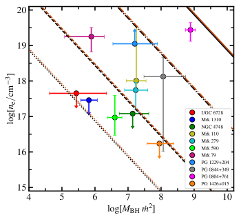
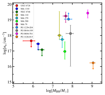
Figure 8: Theoretically, the electron density ($n_{\rm e}$) of the accretion disk depends on five parameters: $M_{\rm BH}$, $\dot{m}$, $f$, $r$, and $r_{\rm in}$. The left panel shows how the disk density changes as a function of the BH mass times the accretion rate squared, $M_{\rm BH}\dot{m}^{2}$ in logarithmic scale. The density solutions for a radiation pressure-dominated disk at $r=6r_{\rm s}$ (in black) and $r=10r_{\rm s}$ (in brown) for $f=0$, $0.7$, $0.95$, and $0.99$ are shown by the dotted, dashed, dash-dotted, and solid lines, respectively. The inner disk radius ($r_{\rm in}$) is set at the sample averaged value of $r_{\rm isco}=2.4r_{\rm s}$. The right panel shows the dependence of $\log n_{\rm e}$ on $\log M_{\rm BH}$ for the sample. There is no evident correlation between these parameters.

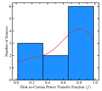
Figure 9: The fraction ($f$) of power transferred from the disk into the corona, measured at $r=10r_{\rm s}$, is plotted as a function of $\log[M_{\rm BH}$ $\dot{m}^{2}$] and $\log[M_{\rm BH}$/$M_{\odot}$] in the left panel. We find a strong positive correlation between $f$ and $\log[M_{\rm BH}$ $\dot{m}^{2}$] with a Spearman rank correlation coefficient of $0.73$ [p-value $=0.01$]. The right panel shows the distribution of the $f$-parameter, which has a median value of $f=0.7_{-0.4}^{+0.2}$.

4.4 Disk Density & Disk-to-Corona Power Transfer Fraction

The electron density of the standard SS73 $\alpha$-disk model (Shakura & Sunyaev, 1973) with a radiation pressure-dominated inner region, including a fraction of power transferred out of the disk to a corona, was derived by Svensson & Zdziarski (1994):

$$n_{\rm e}=\frac{1}{\sigma_{{\rm T}}r_{{\rm s}}}\frac{256\sqrt{2}}{27}\alpha^{-1}r^{3/2}\dot{m}^{-2}\Big{[}1-(r_{{\rm in}}/r)^{1/2}\Big{]}^{-2}(1-f)^{-3},$$ (1)

where $f$ is the disk-to-corona power transfer fraction and represents the fraction of power released from the accretion disk into the corona. The range of the $f$-parameter is $[0,1)$. The $f=0$ solution can provide a non-zero value of the electron density according to SZ94. However, the $f=1$ solution is forbidden in the model. The viscosity parameter is denoted by $\alpha$ and is assumed to be 0.1 (see e.g. Salvesen et al. 2016). The Thomson scattering cross-section is $\sigma_{\rm T}=6.64\times 10^{-25}$ cm². The radius ($r$) of the accretion disk is in the unit of Schwarzschild radius $r_{\rm s}=\frac{2GM_{\rm BH}}{c^{2}}$. The inner disk radius ($r_{\rm in}$) is at the innermost stable circular orbit in the relativistic disk reflection model, the average of which is estimated to be $\langle r_{\rm isco}\rangle\sim 2.4r_{\rm s}$ for the sample. $\dot{m}=\frac{\dot{M}}{\dot{M}_{\rm E}}$ denotes the dimensionless mass accretion rate.

Theoretically, the disk density depends on five parameters: $M_{\rm BH}$, $\dot{m}$, $r_{\rm in}$, $r$, and $f$. The black hole mass and dimensionless mass accretion rate for each source are obtained from the literature and presented in Table 1. In the relativistic reflection model, the inner disk radius ($r_{\rm in}$) is at the innermost stable circular orbit ($r_{\rm isco}$), which can be directly estimated from the black hole spin parameter, reported in Table A2. Therefore, the two unknown parameters involved in the disk density of the standard disk model are the disk-to-corona power transfer fraction ($f$) and radius ($r$) of the accretion disk.

To test the validity of the standard $\alpha$-disk model, we first examine the dependence of disk density on the black hole mass and accretion rate for specific disk radius and $f$-parameter values. Fig. 8 shows the variation in measured disk density with black hole mass times the accretion rate squared ($M_{\rm BH}\dot{m}^{2}$) and black hole mass ($M_{\rm BH}$) in logarithmic scale for the sample. The dotted, dashed, dash-dotted, and solid lines represent the density solutions for $f=0$, $0.7$, $0.95$, and $0.99$, respectively, calculated at $r=6r_{\rm s}$ (in black) and $r=10r_{\rm s}$ (in brown). As evident from Fig. 8 (left panel), the impact of disk radius ($r$) on density is much less than that of the disk-to-corona power transfer fraction, $f$. If the standard $\alpha$-disk theory is valid and the intrinsic scatter associated with the $f$-parameter is negligible, then $\log n_{\rm e}$ and $\log[M_{\rm BH}\dot{m}^{2}]$ have the relation $\log n_{\rm e}\propto-\log[M_{\rm BH}\dot{m}^{2}]$, and we expect an anti-correlation between $\log n_{\rm e}$ and $\log[M_{\rm BH}\dot{m}^{2}]$ as well as between $\log n_{\rm e}$ and $\log M_{\rm BH}$. However, we did not find any correlation between these parameters, which means the intrinsic scatter due to the $f$-parameter is large, and the $f$-values are distinct for different sources in the sample. In principle, disk density is the most influenced by the $f$-parameter with $n_{\rm e}\propto(1-f)^{-3}$ or, $\log n_{\rm e}\propto-3\log(1-f)$. Next, we evaluate the model density for various values of the $f$-parameter as a function of disk radius and compare that with the measured disk density for each source in the sample, as presented in Fig. A6. The model density agrees with the measured density for unique values of the $f$-parameter for different sources. The point of agreement between the model and measured density is found to be at $r=10r_{\rm s}$ for all sources in the sample. Therefore, we calculate the $f$-values from the measured disk density at $r=10r_{\rm s}$ for each source using equation (1) and present them in Table 3. As it stands, we have taken care of all the model intrinsic scatters involved, and if the standard $\alpha$-disk model is valid, we expect a correlation between $f$ and $\log[M_{\rm BH}\dot{m}^{2}]$. In Fig. 9 (left), we show the derived $f$-values for the sample as a function of $\log[M_{\rm BH}\dot{m}^{2}]$ and $\log M_{\rm BH}$. To assess the correlation between these parameters, we perform Spearman’s rank correlation test. The Spearman coefficient value for the $f-\log[M_{\rm BH}\dot{m}^{2}]$ correlation is $\rho_{\rm s}=0.73$, with the null hypothesis (p-value) probability of $0.01$, suggesting a strong positive correlation between these parameters, thus validating the prediction of the standard $\alpha$-disk model with variable disk-to-corona power transfer fraction for the AGN sample. The distribution of the $f$-parameter for the sample is shown in Fig. 9 (right), for which the median value is estimated to be $f=0.7_{-0.4}^{+0.2}$ with $2\sigma$ confidence. From the density solution of SZ94 in equation (1), we notice that if all other input parameters remain constant, the black hole mass with a range of $\log M_{\rm BH}\sim 5.5-9.0$ for the sample can provide around $2$ orders of magnitude variation in disk density. The dimensionless mass accretion rate ($\dot{m}$) of the sample ranges from $\sim 0.1-2.5$ and can alone offer around $3$ orders of magnitude variation in measured density. However, the $f$-parameter varying in the range of $\sim 0.01-0.99$ can cause up to $6$ orders of magnitude variation in the density parameter, justifying a large range of fitted disk densities for the sample.

Table 3: The disk-to-corona power transfer fraction ($f$-parameter) in percent measured at $r=10r_{\rm s}$ for each source in the sample.

Source Name	$f$-parameter [percent]
UGC 6728	$\leq 1.9$
Mrk 1310	$\leq 15.1$
NGC 4748	$\leq 58.9$
Mrk 110	$81.4_{-4.0}^{+12.9}$
Mrk 279	$77.0_{-11.5}^{+3.6}$
Mrk 590	$32.3_{-31.6}^{+25.7}$
Mrk 79	$79.7_{-7.9}^{+3.7}$
PG 1229+204	$\geq 91.4$
PG 0844+349	$90.9_{-36.8}^{+3.1}$
PG 0804+761	$98.2_{-0.5}^{+0.3}$
PG 1426+015	$\leq 57.8$

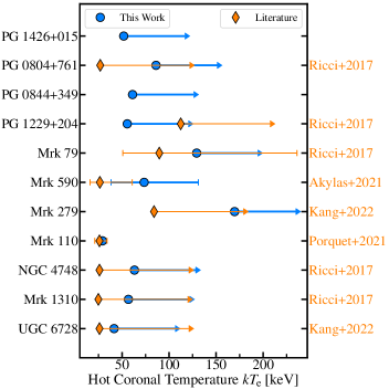
Figure 10: Comparison of the electron temperature (blue circles) of hot corona obtained from our broadband XMM-Newton+NuSTAR spectral modeling of the sample and their previous measurements (orange diamonds) from the literature (Ricci et al. 2017; Akylas & Georgantopoulos 2021; Porquet et al. 2021; Kang & Wang 2022), labeled on the right-hand side of the Y-axis. Orange diamonds are absent for PG 0844+349 and PG 1426+015 since no estimate of their coronal temperature is available in the literature.

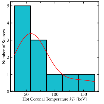
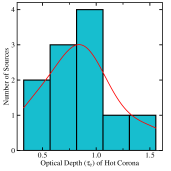
Figure 11: Distribution of measured temperature ($kT_{\rm e}$) and inferred optical depth ($\tau_{\rm e}$) of the hot corona for 11 AGN from this work. The median values of hot coronal temperature and optical depth for the sample are $kT_{\rm e}=63_{-11}^{+23}$ keV and $\tau_{\rm e}=0.85_{-0.27}^{+0.12}$, respectively.

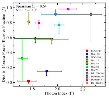
Figure 12: Disk-to-corona power transfer fraction ($f$) as a function of the photon index ($\Gamma$) of the primary continuum. A moderate positive correlation exists between the $f$-parameter and photon index, which can be explained in the context of inverse-Compton scattering of disk photons in the hot corona.

4.5 Coronal Properties and Disk-Corona Interplay

The spectrum of the primary X-ray source or hot corona that illuminates the accretion disk and produces reflection features in the relxillCp and xillverCp models is the thermally Comptoinzed continuum model nthComp. The key parameters of the nthComp model are the spectral shape ($\Gamma$) of the primary continuum and the electron temperature ($kT_{\rm e}$) of the hot corona, which are presented in Table A2. First, we compare the hot coronal temperature measured through our XMM-Newton+NuSTAR broadband spectral modeling of the sample with their previous measurements available in the literature (Ricci et al. 2017; Akylas & Georgantopoulos 2021; Porquet et al. 2021; Kang & Wang 2022), as shown in Figure 10. For AGN when only a cut-off energy ($E_{\rm c}$) estimate is available, we convert it to the electron temperature using $kT_{\rm e}=E_{\rm c}/2.5$ since the cut-off energy of the primary continuum is commonly estimated to be $\sim$2–3 times the electron temperature (Petrucci et al., 2001). No temperature comparison is made for PG 0844+349 and PG 1426+015 since their coronal temperature or cut-off energy measurements are unavailable in the literature. Our broadband spectroscopy provides the first measurement of the coronal temperature in these two AGN. As is evident from Fig. 10, the electron temperature of the hot corona we measure in this work agrees well with that available from the literature within 90% confidence levels. The left panel in Fig. 11 shows our measured temperature distribution of the hot corona for the sample, which has a median value of $63_{-11}^{+23}$ keV with $2\sigma$ confidence.

Another physical parameter that characterizes the corona is the optical depth. However, optical depth is not a free parameter in the nthComp model. Therefore, we need to estimate the optical depth ($\tau_{\rm e}$) of the hot corona, which is related to the electron temperature ($kT_{\rm e}$) and photon index ($\Gamma$) of the nthComp model via the formula:

$$\tau_{\rm e}=\sqrt{2.25+\frac{3}{\frac{kT_{{\rm e}}}{m_{{\rm e}}c^{2}}\times\left[(\Gamma+0.5)^{2}-2.25\right]}}-1.5$$ (2)

The anti-correlation between $kT_{\rm e}$ and $\tau_{\rm e}$ is expected from equation (2) itself. We, therefore, did not perform any correlation analysis between these two parameters. Such correlation analysis is conducted if $\tau_{\rm e}$ is independently measured via models, as shown by Tortosa et al. (2018). The calculated optical depth ($\tau_{\rm e}$) of the hot corona for the sample lies in the range of $\sim 0.3-1.6$, with a mean value of $\sim 0.85$, which agrees well with the AGN employed in Fabian et al. (2015), where the inferred optical depth ranges from $\sim 0.2-1.8$. The distribution of the optical depth for our AGN sample is shown in Fig. 11 (right), the median of which is found at $0.85_{-0.27}^{+0.12}$ with $2\sigma$ confidence. The range of optical depth inferred for the hot corona in this work is reasonable, as demonstrated by the numerical simulations of Haardt & Maraschi (1993). Furthermore, the optical depth of the hot corona is required to be less than one or close to unity for the inner disk relativistic reflection features to be well observed, as argued by Fabian (1994).

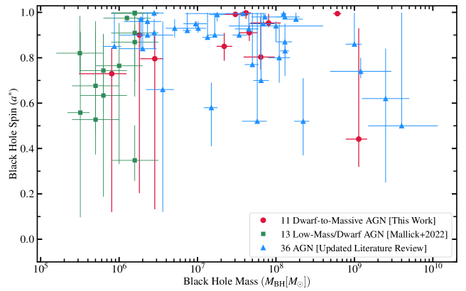
Figure 13: Evolution of dimensionless black hole spin as a function of black hole mass constructed using the most updated spin and mass measurements. The red squares show the spin measurements of the 11 AGN from this work. The green squares and blue triangles denote the spin measurements of the low-mass AGN (including dwarf AGN) from Mallick et al. (2022) and the updated literature review, respectively. The error bars on the measured spin parameter are at 90% confidence levels.

We calculated the disk-to-corona power transfer fraction ($f$) in section 4.4. To further explore the coupling between the accretion disk and corona, we examine the dependence of the $f$-parameter on the photon index ($\Gamma$) of the primary X-ray continuum. Fig. 12 shows the variation in the $f$-parameter with photon index ($\Gamma$), which reveals a moderate positive correlation with a Spearman correlation coefficient of $0.65$ and a null hypothesis (p-value) probability of $0.03$, suggesting that the significance of the observed correlation is marginal yet acceptable. As more photons from the accretion disk are transported into the corona, the number of inverse-Compton scattering increases, considering no changes in disk or coronal geometry. Thus, it makes the corona colder, which results in softer spectra. Likewise, when the corona is extended, it will have a bigger cross-section for scattering photons from the accretion disk. Thus, the corona tends to cool down and the X-ray spectrum gets softer, justifying a positive trend between the photon index and disk-to-corona power transfer fraction.

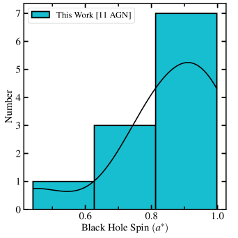
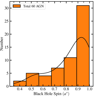
Figure 14: Distribution of black hole spin for 11 AGN from this work and all 60 AGN with updated spin measurements, including those 11 AGN. Our spin measurements increase the spin population by $\sim 20$%.

4.6 Black Hole Spin Measurements from the Relativistic Reflection Features

We estimated the black hole spin by modeling the relativistic reflection features, primarily the broad Fe K line and soft X-ray excess, using the relxillCp model with the assumption that light comes from the innermost stable circular orbit. The accuracy of spin measurements depends on the red wing of the broad Fe K line. We detected a prominent broad Fe K line, which resulted in high spins ($a^{\ast}>0.9$) for most sources in the sample. When the red wing of the broad Fe K line was weak or absent in some AGN (e.g., UGC 6728, Mrk 1310), the spin parameter was found to have large uncertainties. In Fig. 13, we plot the dimensionless black hole spin parameter as a function of black hole mass for 11 AGN from this work, together with the 13 low-mass dwarf AGN from Mallick et al. (2022) and 36 AGN with the most updated spin-mass measurements. With the addition of 11 new spin measurements through joint XMM-Newton/NuSTAR reflection spectroscopy, the total spin sample size has reached $N=60$. Thus, this work is increasing the number of AGN for which a spin measurement is available by around around 20%. The distribution of the black hole spin for our sample is presented in Fig. 14 (left panel), which has a median of $0.89_{-0.09}^{+0.10}$ at the $2\sigma$ confidence level. The right panel in Fig. 14 displays the spin distribution of all $60$ AGN, for which the median is estimated to be $0.88_{-0.05}^{+0.04}$ with $2\sigma$ confidence.

The measurement of high spins is not the shortcoming of the relativistic reflection model. We have previously measured spin parameters in faint dwarf AGN with the same relativistic reflection spectroscopy and obtained low-to-moderate spins (Mallick et al., 2022). A fundamental parameter that is governed by black hole spin is the radiative efficiency of the accretion flow. In the case of a Newtonian disk model, the radiative efficiency can be simplified as

$$\eta\simeq\frac{r_{\rm g}}{2r_{\rm isco}}.$$ (3)

For prograde orbits restricted to $\theta=\pi/2$ plane, the formula for $r_{\rm isco}$ as derived by Bardeen et al. (1972) is:

$$r_{{\rm isco}}=\left(3+Z_{2}-\left[(3-Z_{1})(3+Z_{1}+2Z_{2})\right]^{1/2}\right)r_{{\rm g}},$$ (4)

where,

$$Z_{1}=1+(1-{a^{\ast}}^{2})^{1/3}\left[(1+a^{\ast})^{1/3}+(1-a^{\ast})^{1/3}\right],$$ (5)

$$Z_{2}=\left(3{a^{\ast}}^{2}+Z_{1}^{2}\right)^{1/2}.$$ (6)

As evident from the above equations, the radiative efficiency is purely a function of black hole spin. AGN with high spins ($a^{\ast}>0.9$) have high radiative efficiency ($\eta>0.2$). Not just spin, the radiative efficiency also impacts the luminosity of an accreting object. For a steady-state accretion flow, total radiated luminosity is $L=\eta\dot{M}c^{2}$, where $\dot{M}$ is the accretion rate. Highly spinning black holes have high radiative efficiency, which makes them more luminous even if they have a comparable accretion rate. Therefore, accreting black holes with high spins are more likely to dominate the flux-limited sample (e.g. Vasudevan et al. 2016).

5 Summary & Conclusions

In this paper, we apply the updated higher-density disk reflection model to joint XMM-Newton+NuSTAR broadband spectra of a sample of Type-1 AGN spanning almost the complete range of central black hole mass from $M_{\rm BH}\sim 10^{5.5}M_{\odot}$ to $10^{9}M_{\odot}$. We systematically study the origin of hard and soft X-ray excess for all sources in the sample and, for the first time, verify the relevance of both the high-density disk reflection and warm Comptonization for soft X-ray excess by employing a Bayesian approach. We calculate the disk-to-corona power transfer fraction for the first time in any accreting objects, and probe the accretion disk/corona coupling by exploring its impact on the primary X-ray source or hot corona. Furthermore, we constrain the SMBH spin population across mass scales using broadband reflection spectroscopy. The main results and conclusions of our work are summarized below:

1. The relativistic reflection model from a variable density accretion disk with a broken power-law emissivity profile can describe the soft X-ray excess for 8 out of 11 AGN together with the broad Fe K line and Compton hump whenever detected. A second low-temperature or warm Comptonization component is still required to fit the soft X-ray excess for the remaining 3 sources (NGC 4748, Mrk 110, and PG 1426$+$015) in the sample.

2. The temperature and optical depth of the warm corona measured for those 3 AGN in the sample are measured to be in the range of $T_{\rm wc}\sim 0.25-2$ keV and $\tau_{\rm wc}\sim 4-17$, respectively. Out of these 3 AGN, the measured disk density is significantly higher than the canonical value of $n_{\rm e}=10^{15}$ cm^-3, even with the presence of a warm corona in Mrk 110. This finding is made for the first time in any AGN. For the other two AGN (NGC 4748, PG 1426$+$015), the lower limit of disk density has reached its canonical value.

3. The inner accretion disk of the AGN sample is found to be ionized and dense with a median ionization of $\xi\sim 10^{2.5}$ erg cm^-2 s^-1 and a median density of $n_{\rm e}\sim 10^{17.8}\rm{cm}^{-3}$ without requiring a very high super-solar iron abundance. The iron abundance of the accretion disk is near-solar for the sample, with a median value of $\sim 2$ relative to the solar abundance.

4. We did not find any anti-correlation between the disk density and black hole mass times the accretion rate squared or black hole mass, which implies that the intrinsic scatter in the fraction of power transferred out of the accretion disk to the corona is substantial, and the sample contains diverse disk-to-corona power transfer fractions.

5. For the first time, we calculate the disk-to-corona power transfer fraction for each source, which provides a sample median of $f=0.7_{-0.4}^{+0.2}$ with $2\sigma$ confidence. Moreover, we notice a strong positive correlation between the $f$-parameter and black hole mass times the accretion rate squared, $\log(M_{\rm BH}\dot{m}^{2})$, as expected for a radiation pressure-supported accretion disk.

6. The coupling between the accretion disk and corona is directly evident from the fraction of the disk power transferred into the corona, where the transferred power from the accretion disk can potentially soften the X-ray spectrum of the hot corona. The electron temperature and optical depth of the hot corona are measured to have medians of $63_{-11}^{+23}$ keV and $0.85_{-0.27}^{+0.12}$, respectively, for the sample.

7. With joint XMM-Newton+NuSTAR high-density disk reflection spectroscopy, we are increasing the AGN population for which a spin measurement is available by around 20% across the mass scales of $\log M_{\rm BH}\sim 5.5-9.0$, thus enabling us to achieve a total spin sample size of $60$. We obtain high spins ($a^{\ast}>0.9$) for most sources in the sample when a prominent broad Fe K line is detected. In about 35% of sources in our sample, where the red wing of the broad Fe K line was weak or absent, the measured spin is found to be below $0.9$ with large uncertainties. The median spin of all $60$ AGN is estimated to be $0.88_{-0.05}^{+0.04}$ with $2\sigma$ confidence.

6 Future Prospects

Next-generation X-ray observatories, such as NewAthena (Cruise et al., 2025), AXIS (Reynolds et al., 2023) and Colibrí (Heyl et al., 2020) will significantly advance the scope of this study in multiple ways. Overall, these future missions will allow similar analyses to be performed at a significantly higher redshift, with better accuracy in parameter determination and faster processing.

Focusing on AXIS, which NASA recently selected for Phase A development, its advanced sensitivity in soft X-rays and high spatial resolution will extend the results of this study to fainter AGN populations, thereby probing the disk-to-corona power transfer in lower luminosity regimes, even for non-central, gas-starved supermassive black holes (see e.g. Di Matteo et al. 2023). Overall, AXIS will also provide tighter constraints on the warm and hot coronal temperatures by observing a larger, more diverse sample of AGN across different redshifts and mass scales.

Both NewAthena and AXIS will play a pivotal role in refining spin measurements for a significantly higher number of supermassive black holes (e.g. Cappelluti et al. 2024), especially for high(er)-redshift AGN, which remain underrepresented in current spin demographic studies. Those constraints will also be crucial to improving our knowledge of the population of black hole seeds (e.g. Pacucci & Loeb 2022), typically formed at redshifts $z=20-30$ (Barkana & Loeb, 2001).

Additionally, Colibrí and AXIS will be instrumental in testing competing models for the soft X-ray excess (high-density disk reflection versus warm Comptonization) due to its superior capability to resolve these components spectroscopically. The determination of the X-ray spectral energy distribution of the faint AGN population recently discovered by JWST (see e.g. Harikane et al. 2023) will also open up new possibilities to investigate peculiar spectral shapes and assess the spectral impact of super-Eddington accretors as recently investigated by several studies (see e.g. Pacucci & Narayan 2024).

In summary, several future X-ray facilities, particularly AXIS, will offer immense possibilities for enhancing and expanding the work performed in this paper.

7 acknowledgments

L.M. acknowledges joint support from a CITA National Fellowship (reference #DIS-2022-568580) administered by the University of Toronto and NSERC’s Canada Research Chairs (CRC) Program at the University of Manitoba. L.M. also acknowledges unlimited High-Performance Computing (HPC) support from CITA.

C.P. acknowledges support from PRIN MUR SEAWIND funded by European Union - NextGenerationEU and INAF Grant BLOSSOM.

A.G.M. acknowledges partial support from Narodowe Centrum Nauki (NCN) grants 2018/31/G/ST9/03224 and 2019/35/B/ST9/03944.

S.S.H. acknowledges support from CITA, NSERC’s CRC and Discovery Grant Programs.

F.P. acknowledges support from a Clay Fellowship administered by the Smithsonian Astrophysical Observatory. F.P. also acknowledges support from the BHI Fellowship administered by the Black Hole Initiative at Harvard University.

This research has made use of archival data from XMM-Newton and NuSTAR observatories through the High Energy Astrophysics Science Archive Research Center (HEASARC) Online Service provided by the NASA Goddard Space Flight Center (GSFC). This research has used NuSTAR Data Analysis Software (NuSTARDAS) jointly developed by the ASI Science Data Center (ASDC, Italy) and the California Institute of Technology (USA).

XMM-Newton, NuSTAR

Appendix A Modeling Details of Individual AGN

Here, we discuss the hard-to-soft X-ray spectral fitting details for individual AGN in the sample.

A.0.1 UGC 6728

The source shows a soft X-ray excess below $\sim 2$ keV in XMM-Newton spectra and a broad iron emission line in the 6$-$7 keV range of NuSTAR spectra (Fig. A1). We noticed only a weak Compton hump in the 15$-$30 keV range. Therefore, the hard X-ray (3$-$78 keV) spectral fitting needed mainly the relativistic reflection model (relxillCp) to fit the broad Fe K line, and the model TBabs*(relxillCp+nthComp) provided the best-fit with $\chi^{2}/\rm{dof}=375.8/360$. Once we extrapolate the hard X-ray best-fit model down to 0.3 keV, we find that the relxillCp model can self-consistently fit the soft X-ray excess emission, yielding a very good fit with $\chi^{2}/\rm{dof}=514.7/460$. No structural residuals are seen in the entire energy band. To test the relevance of the warm coronal emission for the origin of soft X-ray excess, we employ a Bayesian approach and added the warm Comptonization model compTT, which provided ${\rm DIC}_{\rm with~WC}=545.2$. The difference between the Deviance Information Criteria without and with the warm Comptonization model is found to be $\Delta{\rm DIC}={\rm DIC}_{\rm without~WC}-{\rm DIC}_{\rm with~WC}=543.9-545.2=-1.3$, implying that an extra warm Comptonization is not required to fit the observed soft X-ray excess in UGC 6728. Considering the LOS Galactic absorption (TBabs), the broadband best-fit model expression is

$${\tt TBabs*(relxillCp+nthComp)}.$$

Fig. A2 shows the broadband 0.3$-$78 keV XMM-Newton/NuSTAR spectra, the best-fit count spectral model with components, and the corresponding residuals. We plot the best-fit spectral energy flux model with relxillCp and nthcomp components in Fig. A3. The best-fit spectral model parameters and their 90% confidence intervals determined through MCMC parameter exploration are presented in Table A2. The best-fit values of disk density, iron abundance, black hole spin, and disk inclination angle are $\log[n_{\rm e}/\rm{cm}^{-3}]\leq 17.7$, $A_{\rm Fe}\leq 4.3$, $a^{\ast}=0.73_{-0.61}^{+0.114}$, and $\theta^{\circ}=50_{-21}^{+4}$, respectively. The temperature of the hot corona is found to be $kT_{\rm e}\geq 42$ keV. The Bayesian analysis suggested no difference between the high-density and canonical disk reflection models, which is supported by the disk density parameter reaching its lower limit of $\log[n_{\rm e}/\rm{cm}^{-3}]=15$.

A.0.2 Mrk 1310

The source revealed only a narrow Fe K_α emission line in the hard X-ray (3$-$78 keV) band (Fig. A1). Compton hump was not detected in the NuSTAR spectra. Therefore, the hard X-ray spectra of Mrk 1310 are best described by the model, TBabs*(zGauss[Narrow]$+$nthComp), with $\chi^{2}/\rm{dof}=199.6/165$. The centroid energy of the Gaussian line is $E_{\rm c}=6.40_{-0.21}^{+0.09}$ keV with the width fixed at $\sigma=10$ eV. It also shows a soft X-ray excess below $\sim 1.5$ keV, which is well-fitted by relxillCp. The model, TBabs*(relxillCp$+$zGauss[Narrow]$+$nthComp), describes the broadband (0.3$-$78 keV) X-ray spectra of Mrk 1310 well with $\chi^{2}/\rm{dof}=272.2/226$. No significant features are seen in the residual plot. We then tested the presence of a warm coronal emission by adding the warm Comptonization model (compTT) and obtained ${\rm DIC}_{\rm with~WC}=311.5$ through the Bayesian analysis. The measured difference between the Deviance Information Criteria without and with warm Comptonization component is $\Delta{\rm DIC}={\rm DIC}_{\rm without~WC}-{\rm DIC}_{\rm with~WC}=299.2-311.5=-12.3<0$. Therefore, the Bayesian model selection metric suggests an extra warm Comptonization is not required to model soft X-ray excess in Mrk 1310. The broadband best-fit model expression, including the LOS Galactic absorption (TBabs), can be written as

$${\tt TBabs*(relxillCp+zGauss[Narrow]+nthComp)}.$$

In Fig. A2, we show the broadband XMM-Newton/NuSTAR spectra, the best-fit count spectral model with components, and the corresponding residual plot. Fig. A3 shows the best-fit spectral energy flux model with relxillCp, zGauss[Narrow], and nthcomp components. In Table A2, we show the best-fit spectral model parameters and their 90% confidence intervals obtained from the MCMC calculation. The best-fit values of disk density, iron abundance, black hole spin, and disk inclination angle are $\log[n_{\rm e}/\rm{cm}^{-3}]\leq 17.5$, $A_{\rm Fe}\leq 3.2$, $a^{\ast}=0.9_{-0.697}^{+0.072}$, and $\theta^{\circ}\leq 50$, respectively. The lower limit on the temperature of the hot corona is estimated to be 57 keV. Most of the parameters remain unconstrained, likely because of the low signal-to-noise of the data. The Bayesian analysis did not find any difference between the high-density and canonical disk reflection models since the density parameter is pegged at the lower bound of $\log[n_{\rm e}/\rm{cm}^{-3}]=15$.

A.0.3 NGC 4748

The XMM-Newton/NuSTAR spectra of NGC 4748 revealed a narrow Fe K_α core at $\sim$ 6.4 keV with a broad Fe K emission feature in the 6$-$7 keV band, a Compton hump above 15 keV, and soft X-ray excess emission below 2 keV, as shown in Fig. A1. The narrow 6.4 keV Fe K_α line and part of the Compton hump are modeled by the distant reflection model xillverCp, while the broad Fe K line and most of the Compton hump are modeled by the relativistic reflection model relxillCp. Therefore, the model, TBabs*(relxillCp$+$xillverCp$+$nthComp), best explains the hard X-ray (3$-$78 keV) spectra with $\chi^{2}/\rm{dof}=207.2/197$. The extrapolation of the hard X-ray best-fit model can fit the broadband (0.3$-$78 keV) X-ray spectra with $\chi^{2}/\rm{dof}=281.0/242$, where the soft X-ray excess is modeled by relxillCp. However, we notice some excess emission in the hard X-ray band, which means relxillCp cannot explain both the soft and hard X-ray excess emission self-consistently. We then add the warm Comptonization model compTT and find that the spectral model, TBabs*(compTT+relxillCp+xillverCp+nthComp), explains the broadband spectra the best with $\chi^{2}/\rm{dof}=258.3/238$. There are no structural residuals in the entire energy band. The Bayesian model selection metric very strongly prefers warm Comptonization over the high-density disk reflection for fitting of soft X-ray excess with $\Delta{\rm DIC}={\rm DIC}_{\rm without~WC}-{\rm DIC}_{\rm with~WC}=306.7-290.6=16.1>10$. Fig. A2 shows the broadband XMM-Newton/NuSTAR spectra, the best-fit count spectral model with components, and the corresponding residual plot. We plot the best-fit spectral energy flux model with compTT, relxillCp, xillverCp, and nthcomp components in Fig. A3. The expression for the broadband best-fit model considering the LOS Galactic absorption (TBabs),

$${\tt TBabs*(compTT+relxillCp+xillverCp+nthComp)}.$$

The best-fit source spectral model parameters and their 90% confidence intervals are obtained through MCMC computation and presented in Table A2. The best-fit values of disk density, iron abundance, black hole spin, and disk inclination angle are estimated to be $\log[n_{\rm e}/\rm{cm}^{-3}]\leq 17.1$, $A_{\rm Fe}\leq 4.9$, $a^{\ast}=0.796_{-0.663}^{+0.123}$, and $\theta^{\circ}=51_{-33}^{+5}$, respectively. We also find a lower limit on the hot coronal electron temperature at 63 keV. Our joint XMM-Newton/NuSTAR spectral modeling better constrained the spin parameter, which was previously not constrained by JJ19’s XMM-Newton spectroscopy alone.

A.0.4 Mrk 110

The source shows soft X-ray excess below $\sim$ 2 keV and a narrow Fe K_α core at $\sim$ 6.37 keV along with a broad iron emission component in the 6$-$7 keV band (Fig. A1). We noticed a hump-like structure around 15$-$30 keV resembling Compton hump, albeit the strength is weak. Therefore, we did not employ the distant reflection model xillverCp and modeled the narrow Fe K_α core using a simple Gaussian line zGauss[Narrow] with the width fixed at $\sigma=10$ eV. The line centroid energy is at $E_{\rm c}=6.37_{-0.02}^{+0.01}$ keV. The broad iron emission feature along with the weak Compton hump are well fitted by the relativistic disk reflection model relxillCp. We find that the model, TBabs*(relxillCp$+$zGauss[Narrow]$+$nthComp), best represents the hard X-ray (3$-$78 keV) spectra of the source with $\chi^{2}/\rm{dof}=1217.0/1154$. By extrapolating the hard X-ray best-fit model down to 0.3 keV, we find that the model is unable to fit the broadband (0.3$-$78 keV) spectra satisfactorily with significant residuals observed in the hard X-ray band, providing $\chi^{2}/\rm{dof}=1901.2/1433$. This suggests that the relativistic reflection model relxillCp cannot self-consistently fit both the soft and hard X-ray excess emission, and an extra warm Comptonization for soft X-ray excess is perhaps needed, as found by Porquet et al. (2024). Hence, we add the warm Comptonization model compTT and find that the model TBabs*(compTT$+$relxillCp$+$zGauss[Narrow]$+$nthComp) represents the broadband spectra well with $\chi^{2}/\rm{dof}=1707.4/1424$, where the soft X-ray excess is fitted by compTT, and relxillCp describes the broad iron emission feature together with the Compton hump. The Bayesian analysis strongly prefers the warm coronal origin of soft X-ray excess over the high-density disk reflection with $\Delta{\rm DIC}={\rm DIC}_{\rm without~WC}-{\rm DIC}_{\rm with~WC}=1995.2-1861.4=133.8>10$. In Fig. A2, we show the broadband XMM-Newton/NuSTAR spectra, the best-fit count spectral model with components, and the corresponding residuals. Fig. A3 presents the best-fit spectral energy flux model with relxillCp, zGauss[Narrow], and nthcomp components. With the LOS Galactic absorption (TBabs), we can write the broadband best-fit model as

$${\tt TBabs*(compTT+relxillCp+xillverCp+nthComp)}.$$

Table A2 presents the best-fit spectral model parameters and their 90% confidence intervals, obtained by exploring the complete parameter space through MCMC. The best-fit values of disk density, iron abundance, black hole spin, and disk inclination angle are $\log[n_{\rm e}/\rm{cm}^{-3}]=18.0_{-0.3}^{+1.5}$, $A_{\rm Fe}\leq 0.8$, $a^{\ast}=0.85_{-0.063}^{+0.059}$, and $\theta^{\circ}=41_{-5}^{+4}$, respectively. The temperature of the hot corona is estimated to be $kT_{\rm e}=29_{-4}^{+4}$ keV. Through joint XMM-Newton/NuSTAR spectroscopy, we can constrain the disk density for which only an upper limit was calculated by JJ19’s XMM-Newton spectral modeling alone. We also show that the Bayesian analysis strongly supports the higher-density disk over the canonical disk reflection model with $\Delta{\rm DIC}>10$.

A.0.5 Mrk 279

The XMM-Newton/NuSTAR spectra of Mrk 279 show two narrow lines at $\sim$ 6.38 keV and $\sim$ 6.95 keV corresponding to Fe K_α and Fe K_β emission lines, respectively, one broad Fe K emission line at $\sim$ 6.7 keV, a mild Compton hump above 15 keV, and a soft X-ray excess below 2 keV (Fig. A1). To fit the hard X-ray (3$-$78 keV) spectra of the source, we employ the model TBabs*(relxillCp$+$xillverCp$+$nthComp), which provided the best-fit with $\chi^{2}/\rm{dof}=1031.3/956$. Here the two narrow Fe K emission lines and part of the Compton hump are modeled by the distant reflection xillverCp, and the relativistic disk reflection model relxillCp fits the broad Fe K emission and most of the Compton hump. Self-consistently, the soft X-ray excess is explained by the relxillCp model, and the hard X-ray best-fit spectral model represents the broadband (0.3$-$78 keV) X-ray spectra well with $\chi^{2}/\rm{dof}=1376.9/1181$. We did not see any additional features or structural residuals in the whole energy band. To test the warm coronal origin of soft X-ray excess, we added the warm Comptonization model compTT to the model TBabs*(relxillCp$+$xillverCp$+$nthComp) and performed a Bayesian analysis, which finds that the difference between the Deviance Information Criteria without and with warm Comptonization is $\Delta{\rm DIC}={\rm DIC}_{\rm without~WC}-{\rm DIC}_{\rm with~WC}=1463.2-1507.5=-44.3<0$. Thus, the Bayesian analysis strongly supports the high-density disk reflection origin of the observed soft X-ray excess in Mrk 279. Including the LOS Galactic absorption (TBabs), the broadband best-fit model expression is

$${\tt TBabs*(relxillCp+xillverCp+nthComp)}.$$

The broadband XMM-Newton/NuSTAR spectra, the best-fit count spectral model along with all components, and the residual plot are shown in Fig. A2. We plot the best-fit spectral energy flux model with relxillCp, xillverCp, and nthcomp components in Fig. A3. We explore the complete parameter space through the MCMC method and list the best-fit source spectral model parameters and their 90% confidence intervals in Table A2. The best-fit values of disk density, iron abundance, black hole spin, and disk inclination angle are $\log[n_{\rm e}/\rm{cm}^{-3}]=17.7_{-0.5}^{+0.2}$, $A_{\rm Fe}=1.8_{-0.4}^{+0.3}$, $a^{\ast}=0.992_{-0.005}^{+0.004}$, and $\theta^{\circ}=31_{-4}^{+4}$, respectively. The lower boundary on the electron temperature of the hot corona is measured at 170 keV. The Bayesian analysis strongly preferred the higher-density disk against the canonical disk with $\Delta{\rm DIC}>10$. The joint XMM-Newton/NuSTAR spectroscopy constrained all the disk reflection model parameters, particularly the disk density and black hole spin, which were not constrained by JJ19’s XMM-Newton spectral fitting of the source, as shown in Fig. 7.

A.0.6 Mrk 590

In the XMM-Newton/NuSTAR spectra of the source, we find a narrow Fe K_α core at $\sim$ 6.38 keV with a broad emission feature in the 6$-$7 keV band and soft X-ray excess below 2 keV (Fig. A1). There is no Compton hump observed in the NuSTAR spectra. The narrow Fe K_α core was fitted by a simple Gaussian line zGauss[Narrow] with the width fixed at $\sigma=10$ eV. The centroid energy of the line is $E_{\rm c}=6.39_{-0.01}^{+0.01}$ keV. We fit the broad iron emission component by the relativistic disk reflection model relxillCp. Therefore, the model TBabs*(relxillCp$+$zGauss[Narrow]$+$nthComp) best describes the hard X-ray (3$-$78 keV) spectra of the source, providing $\chi^{2}/\rm{dof}=1675.7/1642$. Once we extrapolate the hard X-ray best-fit model down to 0.3 keV, the same model can fit the broadband (0.3$-$78 keV) spectra well, providing a reasonable fit with $\chi^{2}/\rm{dof}=2150.1/2047$. Self-consistently, relativistic disk reflection (relxillCp) explains the soft X-ray excess. We then add the warm Comptonization model (compTT) and test its relevance for soft X-ray excess through Bayesian analysis. The estimated difference between the Deviance Information Criteria without and with the warm Comptonization component is $\Delta{\rm DIC}={\rm DIC}_{\rm without~WC}-{\rm DIC}_{\rm with~WC}=2319.3-2341.0=-21.7<0$, confirming that the high-density disk reflection is sufficient enough to fit the observed soft X-ray excess and an extra warm Comptonization is not required. Considering the LOS Galactic absorption (TBabs), the broadband best-fit model expression can written as

$${\tt TBabs*(relxillCp+zGauss[Narrow]+nthComp)}.$$

We show the broadband XMM-Newton/NuSTAR spectra, the best-fit count spectral model with components, and the corresponding residuals in Fig. A2. The best-fit spectral energy flux model with relxillCp, zGauss[Narrow], and nthcomp components are presented in Fig. A3. Table A2 shows the best-fit spectral model parameters and their 90% confidence intervals, where the complete parameter space is explored through MCMC. The best-fit values of disk density, iron abundance, black hole spin, and disk inclination angle are found to be $\log[n_{\rm e}/\rm{cm}^{-3}]=17.0_{-0.5}^{+0.6}$, $A_{\rm Fe}=3.2_{-0.6}^{+0.5}$, $a^{\ast}\geq 0.972$, and $\theta^{\circ}\geq 48$, respectively. The electron temperature of the hot corona is measured to be $kT_{\rm e}=73_{-35}^{+58}$ keV. Through Bayesian analysis, we verify that the higher-density disk is preferred over the canonical disk reflection model with $\Delta{\rm DIC}=8.7$.

A.0.7 Mrk 79

The source Mrk 79 shows two narrow emission lines and one broad emission line in the iron band (6$-$7 keV), a Compton hump in the $\sim 15-30$ keV range, and variable soft X-ray excess emission below $\sim 2$ keV (Fig. A1). The line energies of the two detected narrow lines are at $\sim 6.38$ keV and $\sim 6.95$ keV, which correspond to Fe K_α and Fe K_β emission lines, respectively. The hard X-ray (3$-$78 keV) spectra of the source are best described by the model TBabs*(relxillCp$+$xillverCp$+$nthcomp) with $\chi^{2}/\rm{dof}=715.1/718$, where xillverCp models Fe K_α and Fe K_β emission lines together with the Compton hump and the broad Fe K emission is modeled by relxillCp. When extrapolated down to 0.3 keV, the hard X-ray best-fit model self-consistently fits the broadband (0.3$-$78 keV) X-ray spectra with $\chi^{2}/\rm{dof}=1138.6/972$, where the relativistic disk reflection model relxillCp describes the soft X-ray excess. When we add the warm Comptonization model (compTT) to test the warm coronal origin of soft X-ray excess, the Bayesian model selection metric finds that the difference between the Deviance Information Criteria without and with the warm Comptonization component is $\Delta{\rm DIC}={\rm DIC}_{\rm without~WC}-{\rm DIC}_{\rm with~WC}=1211.0-1296.0=-85.0<0$. Thus, the Bayesian analysis confirms that an extra warm Comptonization over the higher-density disk reflection is not required to explain the soft X-ray excess in Mrk 79. Therefore, we can write the broadband best-fit model expression as

$${\tt TBabs*(relxillCp+xillverCp+nthComp)}.$$

Fig. A2 shows the broadband XMM-Newton/NuSTAR spectra, the best-fit count spectral model with components, and the corresponding residuals. We present the best-fit spectral energy flux model with relxillCp, xillverCp, and nthcomp components in Fig. A3. The best-fit spectral model parameters and their 90% confidence intervals derived through MCMC are presented in Table A2. Our MCMC analysis confirms that all the reflection model parameters are well-constrained with the best-fit values of disk density, iron abundance, black hole spin, and disk inclination angle are $\log[n_{\rm e}/\rm{cm}^{-3}]=19.3_{-0.4}^{+0.3}$, $A_{\rm Fe}=0.9_{-0.2}^{+0.4}$, $a^{\ast}=0.91_{-0.036}^{+0.034}$, and $\theta^{\circ}=36_{-3}^{+4}$, respectively. We obtained more precise and accurate measurements of the black hole spin parameter, which was not constrained by the relativistic reflection spectroscopy of only XMM-Newton spectra (see Fig. 7). The Bayesian model selection metric strongly supports the higher-density disk reflection model against the canonical one with $\Delta{\rm DIC}>10$.

A.0.8 PG 1229+204

The XMM-Newton/NuSTAR spectra of PG 1229+204 unveiled one narrow line at $\sim 6.4$ keV corresponding to Fe K_α emission, a broad Fe K line in the 5$-$7 keV band, a Compton hump above 15 keV, and a strong soft X-ray excess below 2 keV (Fig. A1). The hard X-ray (3$-$78 keV) spectra of the source are best modeled by TBabs*(relxillCp$+$xillverCp$+$nthcomp) with $\chi^{2}/\rm{dof}=122.8/111$. The narrow Fe K_α emission line and most of the Compton hump are fitted by the distant reflection model xillverCp. The relativistic disk reflection model, relxillCp, accounts for the broad Fe K line emission and part of the Compton hump. Once we extrapolate the hard X-ray best-fit model down to 0.3 keV, we can fit the complete 0.3$-$78 keV energy band by the same model, providing a perfect fit with $\chi^{2}/\rm{dof}=152.7/152$ and the relativistic disk reflection (relxillCp) explains the soft X-ray excess self-consistently. However, we still tested the relevance of warm corona for soft X-ray excess and added the warm Comptonization model compTT. The Bayesian analysis finds that the difference between the Deviance Information Criteria without and with the warm Comptonization model is $\Delta{\rm DIC}={\rm DIC}_{\rm without~WC}-{\rm DIC}_{\rm with~WC}=184.7-193.0=-8.3<0$, confirming that the high-density disk reflection is sufficient for the modeling of soft X-ray excess and an additional warm Comptonization component is not required. Considering the LOS Galactic absorption (TBabs), the broadband best-fit model can be written as

$${\tt TBabs*(relxillCp+xillverCp+nthComp)}.$$

The broadband XMM-Newton/NuSTAR spectra, the best-fit count spectral model with components, and the corresponding residual plot are shown in Fig. A2. We plot the best-fit spectral energy flux model with relxillCp, xillverCp, and nthcomp components in Fig. A3. The complete parameter space of the best-fit model was explored using MCMC computation. In Table A2, we present the best-fit spectral model parameters and their 90% confidence intervals. The best-fit values of disk density, iron abundance, black hole spin, and disk inclination angle are $\log[n_{\rm e}/\rm{cm}^{-3}]\geq 19.0$, $A_{\rm Fe}=0.9_{-0.3}^{+1.0}$, $a^{\ast}=0.803_{-0.055}^{+0.175}$, and $\theta^{\circ}=33_{-7}^{+14}$, respectively. The temperature of the hot corona is estimated to be $kT_{\rm e}\geq 56$ keV. As confirmed by our Bayesian analysis, the evidence of the higher-density disk over the canonical disk reflection model is strong with $\Delta{\rm DIC}=6.4$ (Table 2).

A.0.9 PG 0844+349

In the XMM-Newton/NuSTAR spectra of the source, there exists a narrow Fe K_α core at 6.4 keV along with a broad Fe K emission feature in the 5$-$7 keV band, a Compton hump above 10 keV and variable soft X-ray excess below around 1-2 keV (Fig. A1). Therefore, we model the hard X-ray (3$-$78 keV) spectra using TBabs*(relxillCp$+$xillverCp$+$nthcomp), which provided the best-fit with $\chi^{2}/\rm{dof}=87.9/83$. The relativistic disk reflection model relxillCp fits the broad Fe K emission, and the distant reflection model xillverCp fits the narrow Fe K_α core together with the Compton hump. Once the hard X-ray best-fit model is found, we extrapolate it down to 0.3 keV and fit the broadband (0.3$-$78 keV) spectra with that model, which provided a reasonable fit with $\chi^{2}/\rm{dof}=172.0/152$, where the soft X-ray excess is self-consistently modeled by relxillCp. We did not notice any structural residuals in the complete energy band. We then add the warm Comptonization model (compTT) to test the relevance of warm corona for the origin of soft X-ray excess through Bayesian analysis and find that the difference between the Deviance Information Criteria without and with warm Comptonization is $\Delta{\rm DIC}={\rm DIC}_{\rm without~WC}-{\rm DIC}_{\rm with~WC}=225.1-234.5=-9.4<0$. As confirmed by the Bayesian model selection metric, the modeling of soft X-ray excess does not require an additional warm Comptonization over the high-density relativistic disk reflection model. The broadband best-fit model containing the LOS Galactic absorption (TBabs) can be expressed as

$${\tt TBabs*(relxillCp+xillverCp+nthComp)}.$$

Fig. A2 shows the broadband XMM-Newton/NuSTAR spectra, the best-fit count spectral model with components, and the corresponding residuals. In Fig. A3, we present the best-fit spectral energy flux model with relxillCp, xillverCp, and nthcomp components. The best-fit spectral model parameters and their 90% confidence intervals are presented in Table A2, where we explore the complete parameter space and calculate the parameter uncertainties using the MCMC method. The best-fit values of disk density, iron abundance, black hole spin, and disk inclination angle are $\log[n_{\rm e}/\rm{cm}^{-3}]=18.1_{-2.1}^{+0.5}$, $A_{\rm Fe}\leq 3.2$, $a^{\ast}=0.953_{-0.019}^{+0.04}$, and $\theta^{\circ}\leq 41$, respectively. The estimated lower limit of the hot coronal temperature is at 61 keV. Our Bayesian analysis suggests that the evidence of the higher-density disk against the canonical disk reflection model is positive with $\Delta{\rm DIC}=3.3$ (Table 2).

A.0.10 PG 0804+761

The source revealed a narrow Fe K_α emission line at $\sim 6.4$ keV with a broad emission feature in the 5$-$7 keV band, a Compton hump above 15 keV, and a soft X-ray excess below 2 keV, as shown in Fig. A1. To fit the narrow Fe K_α line emission and Compton hump, we employ the distant reflection model xillverCp. We fit the broad iron emission feature with the relativistic disk reflection model relxillCp. Therefore, the hard X-ray (3$-$78 keV) spectral data of the source are best described by the model, TBabs*(relxillCp$+$xillverCp$+$nthcomp), with $\chi^{2}/\rm{dof}=159.3/192$. We extrapolated the same model down to 0.3 keV and successfully fit broadband (0.3$-$78 keV) spectral data, which provided a perfect fit with $\chi^{2}/\rm{dof}=267.4/278$. No features are seen in the residual spectra. Self-consistently, the relativistic reflection model (relxillCp) can explain the soft X-ray excess emission in the source. However, we still investigate the warm coronal origin of soft X-ray excess and add the warm Comptonization model compTT. As found by our Bayesian analysis, the difference between the Deviance Information Criteria without and with warm Comptonization is $\Delta{\rm DIC}={\rm DIC}_{\rm without~WC}-{\rm DIC}_{\rm with~WC}=295.6-298.5=-3.0<0$, confirming the high-density disk reflection origin of soft X-ray excess. The broadband best-fit model expression incorporating the LOS Galactic absorption (TBabs) is

$${\tt TBabs*(relxillCp+xillverCp+nthComp)}.$$

In Fig. A2, we show the broadband XMM-Newton/NuSTAR spectra, the best-fit count spectral model with components, and the corresponding residual plot. The best-fit source spectral energy flux model with components are plotted in Fig. A3. In Table A2, we present the best-fit spectral model parameters and their 90% confidence intervals obtained through MCMC parameter space exploration of the best-fit model. The best-fit values of disk density, iron abundance, black hole spin, and disk inclination angle are estimated to be $\log[n_{\rm e}/\rm{cm}^{-3}]=19.4_{-0.3}^{+0.2}$, $A_{\rm Fe}=0.6_{-0.1}^{+0.1}$, $a^{\ast}=0.995_{-0.007}^{+0.003}$, and $\theta^{\circ}=28_{-7}^{+5}$, respectively. We measured a lower limit on the electron temperature of the hot corona at 86 keV. We obtain constraints on both the disk density and black hole spin parameters, which were not constrained through the XMM-Newton spectral modeling alone, as depicted in Fig. 3. Through Bayesian analysis, we confirm that the evidence of the higher-density disk against the canonical disk reflection is very strong with $\Delta{\rm DIC}>10$.

A.0.11 PG 1426+015

In the XMM-Newton/NuSTAR spectra of the source, we detect a narrow line at $\sim 6.4$ keV corresponding to the Fe K_α emission along with a broad iron emission feature in the 6$-$7 keV band, a strong Compton hump in the 15$-$30 keV range, and a soft X-ray excess below 2 keV (see Fig. A1). We model the hard X-ray (3$-$78 keV) spectra of the source with TBabs*(relxillCp$+$xillverCp$+$nthcomp) and obtain the best-fit with $\chi^{2}/\rm{dof}=372.8/349$. The distant reflection model (xillverCp) explains the narrow Fe K_α line emission and part of the Compton hump. The broad Fe K feature and most of the Compton hump are described by the relativistic reflection model relxillCp. The extrapolation of the hard X-ray best-fit model is unable to explain the broadband (0.3$-$78 keV) X-ray spectra well, yielding $\chi^{2}/\rm{dof}=524.9/420$ with significant residuals in the hard X-ray band which implies that the relxillCp model cannot fit both soft and hard X-ray excess self-consistently. Therefore, we add the warm Comptonization model (compTT) for soft X-ray excess and find that the model TBabs*(compTT+relxillCp+xillverCp+nthComp) fits the broadband spectra well with $\chi^{2}/\rm{dof}=477.8/415$. No structures or features are seen in the residual spectra. The Bayesian model selection metric confirms the relevance of warm Comptonization over the high-density disk reflection for soft X-ray excess since the difference between the Deviance Information Criteria without and with the warm Comptonization component is $\Delta{\rm DIC}={\rm DIC}_{\rm without~WC}-{\rm DIC}_{\rm with~WC}=575.8-534.6=41.2>0$. We can write the broadband best-fit model considering the LOS Galactic absorption (TBabs) as

$${\tt TBabs*(compTT+relxillCp+xillverCp+nthComp)}.$$

Fig. A2 shows the broadband XMM-Newton/NuSTAR spectra, the best-fit count spectral model with components, and the corresponding residuals. We plot the best-fit source spectral energy flux model with all four (compTT, relxillCp, xillverCp, and nthcomp) components in Fig. A3. Our MCMC analysis explored the complete parameter space of the best-fit model. The resulting best-fit spectral model parameters and their 90% confidence intervals are presented in Table A2. The best-fit values of disk density, iron abundance, black hole spin, and disk inclination angle are $\log[n_{\rm e}/\rm{cm}^{-3}]\leq 16.2$, $A_{\rm Fe}=1.6_{-0.7}^{+0.9}$, $a^{\ast}=0.442_{-0.122}^{+0.488}$, and $\theta^{\circ}=22_{-6}^{+27}$, respectively. We measured the electron temperature of the hot corona at $kT_{\rm e}\geq 52$ keV. While performing the XMM-Newton spectral modeling of the source, JJ19 fixed the spin parameter at 0.998. Through joint XMM-Newton/NuSTAR relativistic reflection spectroscopy, we provide the first measurement of the black hole spin parameter for PG 1426+015.

Table 4: Observing Log of the AGN sample.

Source	Observatory	Camera	Obs. ID	Start Time	Elapsed Time	Net Exposure	Net Count Rate	Net Counts
				[MJD]	[ks]	[ks]	[ct/s]
UGC 6728	XMM-Newton	EPIC-MOS1	0312191601	53789.8	12.15	8.22	0.87	7.16E+03
		EPIC-MOS2			11.58	8.74	0.87	7.60E+03
	NuSTAR	FPMA	60376007002	58039.8	68.39	51.80	0.40	2.07E+04
		FPMB				50.73	0.37	1.86E+04
		FPMA	60160450002	57579.5	27.59	21.20	0.19	3.95E+03
		FPMB				21.36	0.17	3.72E+03
Mrk 1310	XMM-Newton	EPIC-pn	0831790501	58487.3	24.16	16.32	1.76	2.88E+04
		EPIC-pn	0723100301	56635.4	55.18	33.74	0.15	4.97E+03
	NuSTAR	FPMA	60160465002	57556.5	38.57	21.13	0.23	4.86E+03
		FPMB				21.08	0.21	4.49E+03
NGC 4748	XMM-Newton	EPIC-pn	0723100401	56671.3	65.38	26.42	4.21	1.11E+05
	NuSTAR	FPMA	60663002002	59238.4	154.82	79.91	0.18	1.41E+04
		FPMB				79.07	0.16	1.27E+04
Mrk 110	XMM-Newton	EPIC-pn	0201130501	53324.2	46.97	32.30	21.18	6.84E+05
		EPIC-pn	0852590101	58804.4	42.64	29.03	19.48	5.65E+05
		EPIC-pn	0852590201	58946.0	46.64	31.69	15.23	4.83E+05
		EPIC-pn	0840220801	58792.4	41.14	28.37	14.53	4.12E+05
		EPIC-pn	0840220901	58794.4	38.74	26.35	15.48	4.08E+05
		EPIC-pn	0840220701	58790.4	41.74	28.41	10.07	2.86E+05
	NuSTAR	FPMA	60201025002	57776.8	386.30	177.33	1.09	1.93E+05
		FPMB				176.53	1.03	1.82E+05
		FPMA	60502022002	58803.2	163.20	86.77	0.75	6.50E+04
		FPMB				85.97	0.69	5.93E+04
		FPMA	60502022004	58944.6	168.44	88.67	0.64	5.66E+04
		FPMB				87.75	0.59	5.15E+04
Mrk 279	XMM-Newton	EPIC-pn	0302480401	53689.7	59.37	40.58	19.33	7.85E+05
		EPIC-pn	0302480501	53691.7	59.37	37.76	16.56	6.25E+05
		EPIC-pn	0302480601	53694.0	37.77	21.76	17.50	3.81E+05
		EPIC-pn	0872391301	59203.3	28.64	19.60	11.47	2.25E+05
		EPIC-pn	0083960101	52401.5	30.07	13.00	3.22	4.19E+04
	NuSTAR	FPMA	60601011004	59066.5	317.27	199.41	0.16	3.21E+04
		FPMB				197.85	0.14	2.77E+04
		FPMA	60160562002	58785.4	37.75	27.28	0.66	1.81E+04
		FPMB				27.07	0.63	1.71E+04
		FPMA	60601011006	59073.0	79.61	52.38	0.21	1.09E+04
		FPMB				51.97	0.19	9.94E+03
		FPMA	60601011002	59064.9	97.04	58.24	0.17	9.74E+03
		FPMB				58.05	0.15	8.58E+03
Mrk 590	XMM-Newton	EPIC-pn	0201020201	53190.9	61.45	41.85	3.37	1.41E+05
		EPIC-pn		53190.4	45.31	29.23	3.17	9.27E+04
		EPIC-pn	0865470301	59217.5	25.14	17.10	3.84	6.56E+04
		EPIC-pn	0865470201	59034.6	25.14	17.25	3.23	5.58E+04
		EPIC-pn	0870840301	59981.2	36.14	24.73	2.01	4.97E+04
		EPIC-pn	0912400101	59788.4	25.14	17.26	2.75	4.75E+04
		EPIC-pn	0870840101	59437.1	8.94	6.04	5.65	3.41E+04
		EPIC-pn	0870840401	59439.1	5.34	3.64	6.69	2.43E+04
		EPIC-pn	0870840201	59603.1	23.94	16.34	1.12	1.83E+04
		EPIC-pn	0109130301	52275.5	10.00	6.80	2.43	1.65E+04
	NuSTAR	FPMA	80502630002	58726.4	136.75	65.02	0.35	2.29E+04
		FPMB				64.05	0.31	2.00E+04
		FPMA	80502630004	58869.5	97.75	50.03	0.36	1.79E+04
		FPMB				49.64	0.33	1.66E+04
		FPMA	80502630006	59224.5	84.21	41.26	0.17	7.13E+03
		FPMB				41.00	0.16	6.41E+03
		FPMA	80602604002	59571.0	114.55	53.05	0.13	7.05E+03
		FPMB				52.42	0.12	6.41E+03
		FPMA	60761012002	59444.2	39.76	18.65	0.34	6.40E+03
		FPMB				16.96	0.32	5.39E+03
		FPMA	80402610002	58418.4	38.50	21.07	0.25	5.26E+03
		FPMB				20.96	0.23	4.78E+03
		FPMA	80602604004	59981.1	84.75	40.58	0.12	4.69E+03
		FPMB				39.88	0.11	4.31E+03
		FPMA	90201043002	57724.5	95.57	50.62	0.08	4.20E+03
		FPMB				50.45	0.07	3.46E+03
		FPMA	60160095002	57423.7	39.03	21.21	0.08	1.60E+03
		FPMB				21.16	0.07	1.39E+03
Mrk 79	XMM-Newton	EPIC-pn	0870880101	59117.6	29.64	20.11	12.72	2.56E+05
		EPIC-pn	0400070201	54008.5	20.67	13.84	15.11	2.09E+05
		EPIC-pn	0400070401	54178.1	20.31	13.57	10.24	1.39E+05
		EPIC-pn	0400070301	54040.6	19.97	13.92	9.95	1.39E+05
		EPIC-pn	0103860801	51826.2	2.41	1.61	11.46	1.84E+04
		EPIC-pn	0103862101	52025.8	5.12	3.52	5.21	1.83E+04
	NuSTAR	FPMA	60601010002	59115.5	125.42	64.44	0.63	4.08E+04
		FPMB				64.45	0.58	3.72E+04
		FPMA	60601010004	59117.2	73.09	38.19	0.65	2.47E+04
		FPMB				38.10	0.59	2.25E+04
PG 1229+204	XMM-Newton	EPIC-pn	0301450201	53560.5	25.07	17.17	2.74	4.71E+04
	NuSTAR	FPMA	60061229002	57597.4	37.52	18.61	0.09	1.75E+03
		FPMB				18.39	0.09	1.58E+03
PG 0844+349	XMM-Newton	EPIC-pn	0103660201	51853.0	21.24	5.98	2.38	1.43E+04
		EPIC-pn	0554710101	54954.2	12.67	11.33	0.42	4.72E+03
	NuSTAR	FPMA	60463024002	59224.0	41.43	17.70	0.05	8.14E+02
		FPMB				17.59	0.04	7.46E+02
PG 0804+761	XMM-Newton	EPIC-pn	0605110101	55265.5	44.50	16.18	10.36	1.68E+05
		EPIC-pn	0605110201	55267.5	36.25	15.56	7.88	1.23E+05
	NuSTAR	FPMA	60160322002	57480.1	26.30	16.94	0.18	3.13E+03
		FPMB				16.87	0.18	2.96E+03
PG 1426+015	XMM-Newton	EPIC-pn	0852210101	58872.5	106.14	70.48	3.05	2.15E+05
		EPIC-pn	0102040501	51753.5	6.06	0.68	4.16	2.85E+03
	NuSTAR	FPMA	60501049002	58871.9	202.55	94.12	0.17	1.56E+04
		FPMB				93.82	0.16	1.48E+04
		FPMA	60061254002	58340.4	62.21	32.48	0.20	6.62E+03
		FPMB				32.32	0.19	6.05E+03

Table A2: The best-fit model parameters obtained from the joint fitting of the broadband (0.3$-$78 keV) XMM-Newton+NuSTAR spectra for each source.

Object Name: Source Spectral Model with Components
UGC 6728: Model $\equiv$ relxillCp [relativistic reflection] $+$ nthComp [hot corona]
	$T_{\rm start}$	$q_{\rm in}$	$\theta$	$a^{\ast}$	$\log n_{\rm e}$	$A_{\rm Fe}$	$\log\xi$	$F_{\rm rel}$	$\Gamma$	$kT_{\rm e}$	$F_{\rm nth}$	$\frac{\chi^{2}}{d.o.f}$
EPIC	$53789.8$	$\geq 3.3$	$50_{-21}^{+4}$	$0.73_{-0.61}^{+0.114}$	$\leq 17.7$	$\leq 4.3$	$1.8_{-1.2}^{+0.7}$	$8.4_{-1.7}^{+1.7}$	$1.82_{-0.09}^{+0.04}$	$\geq 42$	$18.1_{-0.5}^{+0.5}$	$\frac{514.7}{460}$
FPM	$58039.8$	$-$	$50^{\ast}$	$0.73^{\ast}$	$-$	$4.2^{\ast}$	$1.8^{\ast}$	$7.5_{-0.9}^{+0.9}$	$1.78_{-0.05}^{+0.07}$	$-$	$45.1_{-0.9}^{+0.8}$
FPM	$57579.5$	$-$	$50^{\ast}$	$0.73^{\ast}$	$-$	$4.2^{\ast}$	$1.8^{\ast}$	$2.5_{-1.1}^{+1.1}$	$1.71_{-0.12}^{+0.08}$	$-$	$23.9_{-1.0}^{+1.0}$
Mrk 1310: Model $\equiv$ relxillCp [relativistic reflection] $+$ nthComp [hot corona] $+$ zGauss[Narrow Fe Kα emission line]
	$T_{\rm start}$	$q_{\rm in}$	$\theta^{\circ}$	$a^{\ast}$	$\log n_{\rm e}$	$A_{\rm Fe}$	$\log\xi$	$F_{\rm rel}$	$\Gamma$	$kT_{\rm e}$	$F_{\rm nth}$	$E_{\rm c}$	$F_{\rm NGa}$	$\frac{\chi^{2}}{d.o.f}$
EPIC	$58487.3$	$5.1_{-1.7}^{+4.5}$	$\leq 50$	$0.9_{-0.697}^{+0.072}$	$\leq 17.5$	$\leq 3.2$	$\leq 0.5$	$4.0_{-0.5}^{+0.5}$	$1.99_{-0.08}^{+0.04}$	$\geq 57$	$8.0_{-0.1}^{+0.1}$	$6.42_{-0.2}^{+0.07}$	$1.2_{-0.2}^{+0.8}$	$\frac{272.2}{226}$
EPIC	$56635.4$	$5.1^{\ast}$	$-$	$0.9^{\ast}$	$-$	$-$	$-$	$0.6_{-0.2}^{+0.2}$	$1.98_{-0.11}^{+0.07}$	$-$	$0.6_{-0.02}^{+0.02}$	$6.42^{\ast}$	$1.2^{\ast}$
FPM	$57556.5$	$5.1^{\ast}$	$-$	$0.9^{\ast}$	$-$	$-$	$-$	$\leq 1.0$	$1.77_{-0.03}^{+0.24}$	$-$	$30.8_{-1.1}^{+0.7}$	$6.42^{\ast}$	$1.2^{\ast}$
NGC 4748: Model $\equiv$ relxillCp [relativistic reflection] $+$ nthComp [hot corona] $+$ xillverCp [distant reflection] $+$ CompTT [warm corona]
	$T_{\rm start}$	$q_{\rm in}$	$\theta^{\circ}$	$a^{\ast}$	$\log n_{\rm e}$	$A_{\rm Fe}$	$\log\xi$	$F_{\rm rel}$	$\Gamma$	$kT_{\rm e}$	$F_{\rm nth}$	$F_{\rm xil}$	$kT_{\rm wc}$	$\tau_{\rm wc}$	$F_{\rm wc}$	$\frac{\chi^{2}}{d.o.f}$
EPIC	$56671.3$	$\geq 3.3$	$51_{-33}^{+5}$	$0.796_{-0.663}^{+0.123}$	$\leq 17.1$	$\leq 4.9$	$3.1_{-0.7}^{+0.7}$	$3.5_{-1.5}^{+1.5}$	$1.77_{-0.21}^{+0.11}$	$\geq 63$	$23.2_{-1.0}^{+1.0}$	$1.0_{-0.6}^{+0.6}$	$1.8_{-1.0}^{+0.2}$	$4.0_{-0.7}^{+2.5}$	$12.9_{-1.1}^{+2.5}$	$\frac{258.3}{238}$
FPM	$59238.4$	$-$	$51^{\ast}$	$0.796^{\ast}$	$-$	$-$	$3.1^{\ast}$	$5.5_{-2.4}^{+1.7}$	$1.88_{-0.13}^{+0.17}$	$-$	$22.5_{-1.1}^{+1.3}$	$\leq 0.9$	$-$	$4.0^{\ast}$	$0.5_{-0.4}^{+0.1}$
Mrk 110: Model $\equiv$ relxillCp [relativistic reflection] $+$ nthComp [hot corona] $+$ zGauss[Narrow Fe Kα emission line] $+$ CompTT [warm corona]
	$T_{\rm start}$	$q_{\rm in}$	$\theta^{\circ}$	$a^{\ast}$	$\log n_{\rm e}$	$A_{\rm Fe}$	$\log\xi$	$F_{\rm rel}$	$\Gamma$	$kT_{\rm e}$	$F_{\rm nth}$	$E_{\rm c}$	$F_{\rm NGa}$	$kT_{\rm wc}$	$\tau_{\rm wc}$	$F_{\rm wc}$	$\frac{\chi^{2}}{d.o.f}$
EPIC	$53324.2$	$\geq 8.6$	$41_{-5}^{+4}$	$0.85_{-0.063}^{+0.059}$	$18.0_{-0.3}^{+1.5}$	$\leq 0.8$	$3.0_{-0.2}^{+0.1}$	$10.8_{-0.9}^{+0.9}$	$1.76_{-0.01}^{+0.01}$	$29_{-4}^{+4}$	$85.8_{-0.7}^{+0.7}$	$6.37_{-0.02}^{+0.01}$	$11.1_{-3.7}^{+3.1}$	$0.26_{-0.01}^{+0.02}$	$15.9_{-1.3}^{+0.7}$	$9.7_{-0.7}^{+0.4}$	$\frac{1707.4}{1424}$
EPIC	$58804.4$	$-$	$41^{\ast}$	$0.85^{\ast}$	$18.0^{\ast}$	$-$	$3.0^{\ast}$	$9.4_{-0.9}^{+0.9}$	$1.80_{-0.01}^{+0.01}$	$29^{\ast}$	$74.9_{-0.7}^{+0.7}$	$6.37^{\ast}$	$16.8_{-2.6}^{+2.3}$	$0.26^{\ast}$	$15.9^{\ast}$	$9.1_{-0.5}^{+0.4}$
EPIC	$58946.0$	$-$	$41^{\ast}$	$0.85^{\ast}$	$18.0^{\ast}$	$-$	$3.0^{\ast}$	$4.3_{-0.8}^{+0.8}$	$1.76_{-0.01}^{+0.01}$	$29^{\ast}$	$71.0_{-0.6}^{+0.6}$	$6.37^{\ast}$	$11.6_{-2.3}^{+2.0}$	$0.26^{\ast}$	$15.9^{\ast}$	$6.0_{-0.3}^{+0.4}$
EPIC	$58792.4$	$-$	$41^{\ast}$	$0.85^{\ast}$	$18.0^{\ast}$	$-$	$3.0^{\ast}$	$5.9_{-1.1}^{+1.1}$	$1.78_{-0.01}^{+0.01}$	$29^{\ast}$	$79.5_{-0.8}^{+0.9}$	$6.37^{\ast}$	$9.8_{-4.4}^{+3.3}$	$0.26^{\ast}$	$15.9^{\ast}$	$9.0_{-0.4}^{+0.7}$
EPIC	$58794.4$	$-$	$41^{\ast}$	$0.85^{\ast}$	$18.0^{\ast}$	$-$	$3.0^{\ast}$	$7.0_{-1.2}^{+1.2}$	$1.80_{-0.01}^{+0.01}$	$29^{\ast}$	$80.6_{-0.9}^{+0.9}$	$6.37^{\ast}$	$13.3_{-4.3}^{+3.5}$	$0.26^{\ast}$	$15.9^{\ast}$	$9.3_{-0.5}^{+0.7}$
EPIC	$58790.4$	$-$	$41^{\ast}$	$0.85^{\ast}$	$18.0^{\ast}$	$-$	$3.0^{\ast}$	$3.4_{-0.8}^{+0.8}$	$1.69_{-0.01}^{+0.01}$	$29^{\ast}$	$66.5_{-0.6}^{+0.7}$	$6.37^{\ast}$	$13.3_{-3.7}^{+3.0}$	$0.26^{\ast}$	$15.9^{\ast}$	$6.6_{-0.3}^{+0.6}$
FPM	$57776.8$	$-$	$41^{\ast}$	$0.85^{\ast}$	$18.0^{\ast}$	$-$	$3.0^{\ast}$	$7.3_{-4.8}^{+4.8}$	$1.81_{-0.01}^{+0.01}$	$29^{\ast}$	$126.1_{-4.2}^{+4.2}$	$6.37^{\ast}$	$19.9_{-3.2}^{+3.0}$	$0.26^{\ast}$	$15.9^{\ast}$	$\leq 0.9$
FPM	$58803.2$	$-$	$41^{\ast}$	$0.85^{\ast}$	$18.0^{\ast}$	$-$	$3.0^{\ast}$	$9.4^{\ast}$	$1.80^{\ast}$	$29^{\ast}$	$74.9^{\ast}$	$6.37^{\ast}$	$16.8^{\ast}$	$0.26^{\ast}$	$15.9^{\ast}$	$9.1^{\ast}$
FPM	$58944.6$	$-$	$41^{\ast}$	$0.85^{\ast}$	$18.0^{\ast}$	$-$	$3.0^{\ast}$	$4.3^{\ast}$	$1.76^{\ast}$	$29^{\ast}$	$71.0^{\ast}$	$6.37^{\ast}$	$11.6^{\ast}$	$0.26^{\ast}$	$15.9^{\ast}$	$6.0^{\ast}$
Mrk 279: Model $\equiv$ relxillCp [relativistic reflection] $+$ nthComp [hot corona] $+$ xillverCp [distant reflection]
	$T_{\rm start}$	$q_{\rm in}$	$\theta^{\circ}$	$a^{\ast}$	$\log n_{\rm e}$	$A_{\rm Fe}$	$\log\xi$	$F_{\rm rel}$	$\Gamma$	$kT_{\rm e}$	$F_{\rm nth}$	$F_{\rm xil}$	$\frac{\chi^{2}}{d.o.f}$
EPIC	$53689.7$	$7.8_{-0.3}^{+0.6}$	$31_{-4}^{+4}$	$0.991_{-0.004}^{+0.004}$	$17.7_{-0.5}^{+0.2}$	$1.8_{-0.4}^{+0.3}$	$2.0_{-0.1}^{+0.2}$	$21.1_{-0.7}^{+0.7}$	$2.06_{-0.01}^{+0.02}$	$\geq 170$	$64.6_{-0.4}^{+0.4}$	$8.8_{-0.9}^{+0.9}$	$\frac{1376.9}{1181}$
EPIC	$53691.7$	$7.8^{\ast}$	$31^{\ast}$	$0.991^{\ast}$	$17.7^{\ast}$	$1.8^{\ast}$	$2.0^{\ast}$	$19.3_{-0.7}^{+0.7}$	$2.02_{-0.01}^{+0.02}$	$-$	$59.0_{-0.4}^{+0.4}$	$8.4_{-0.9}^{+0.9}$
EPIC	$53694.0$	$7.8^{\ast}$	$31^{\ast}$	$0.991^{\ast}$	$17.7^{\ast}$	$1.8^{\ast}$	$2.0^{\ast}$	$17.6_{-0.9}^{+0.9}$	$2.06_{-0.01}^{+0.02}$	$-$	$60.0_{-0.5}^{+0.5}$	$9.8_{-1.2}^{+1.2}$
EPIC	$59203.3$	$7.8^{\ast}$	$31^{\ast}$	$0.991^{\ast}$	$17.7^{\ast}$	$1.8^{\ast}$	$2.0^{\ast}$	$10.7_{-0.8}^{+0.8}$	$2.05_{-0.01}^{+0.02}$	$-$	$38.9_{-0.4}^{+0.4}$	$5.8_{-1.0}^{+1.0}$
EPIC	$52401.5$	$7.8^{\ast}$	$31^{\ast}$	$0.991^{\ast}$	$17.7^{\ast}$	$1.8^{\ast}$	$2.0^{\ast}$	$12.5_{-2.0}^{+2.0}$	$2.07_{-0.02}^{+0.02}$	$-$	$40.1_{-1.1}^{+1.1}$	$5.5_{-2.4}^{+2.5}$
FPM	$59066.5$	$7.8^{\ast}$	$31^{\ast}$	$0.991^{\ast}$	$17.7^{\ast}$	$1.8^{\ast}$	$2.0^{\ast}$	$3.8_{-0.5}^{+0.5}$	$1.96_{-0.04}^{+0.05}$	$-$	$15.2_{-0.6}^{+0.6}$	$5.5_{-0.4}^{+0.4}$
FPM	$58785.4$	$7.8^{\ast}$	$31^{\ast}$	$0.991^{\ast}$	$17.7^{\ast}$	$1.8^{\ast}$	$2.0^{\ast}$	$6.4_{-2.6}^{+2.6}$	$2.02_{-0.07}^{+0.05}$	$-$	$74.8_{-2.9}^{+2.9}$	$10.4_{-1.4}^{+1.5}$
FPM	$59073.0$	$7.8^{\ast}$	$31^{\ast}$	$0.991^{\ast}$	$17.7^{\ast}$	$1.8^{\ast}$	$2.0^{\ast}$	$3.0_{-1.1}^{+1.1}$	$1.86_{-0.08}^{+0.06}$	$-$	$23.5_{-1.2}^{+1.3}$	$5.1_{-0.8}^{+0.8}$
FPM	$59064.9$	$7.8^{\ast}$	$31^{\ast}$	$0.991^{\ast}$	$17.7^{\ast}$	$1.8^{\ast}$	$2.0^{\ast}$	$6.1_{-1.1}^{+1.1}$	$2.01_{-0.06}^{+0.09}$	$-$	$14.7_{-1.2}^{+1.2}$	$5.0_{-0.7}^{+0.7}$
Mrk 590: Model $\equiv$ relxillCp [relativistic reflection] $+$ nthComp [hot corona] $+$ zGauss[Narrow Fe Kα emission line]
	$T_{\rm start}$	$q_{\rm in}$	$\theta^{\circ}$	$a^{\ast}$	$\log n_{\rm e}$	$A_{\rm Fe}$	$\log\xi$	$F_{\rm rel}$	$\Gamma$	$kT_{\rm e}$	$F_{\rm nth}$	$E_{\rm c}$	$F_{\rm NGa}$	$\frac{\chi^{2}}{d.o.f}$
EPIC	$53190.9$	$\geq 7.7$	$\geq 48$	$\geq 0.972$	$17.0_{-0.5}^{+0.6}$	$3.2_{-0.6}^{+0.5}$	$2.7_{-0.1}^{+0.1}$	$4.1_{-0.3}^{+0.3}$	$1.70_{-0.01}^{+0.01}$	$73_{-35}^{+58}$	$21.3_{-0.2}^{+0.3}$	$6.39_{-0.01}^{+0.01}$	$8.5_{-1.9}^{+1.8}$	$\frac{2150.1}{2047}$
EPIC	$59217.5$	$-$	$-$	$-$	$17.0^{\ast}$	$3.2^{\ast}$	$2.7^{\ast}$	$5.5_{-0.4}^{+0.4}$	$1.70_{-0.01}^{+0.02}$	$73^{\ast}$	$23.5_{-0.4}^{+0.4}$	$6.39^{\ast}$	$10.2_{-3.5}^{+3.0}$
EPIC	$59034.6$	$-$	$-$	$-$	$17.0^{\ast}$	$3.2^{\ast}$	$2.7^{\ast}$	$3.9_{-0.4}^{+0.4}$	$1.71_{-0.01}^{+0.02}$	$73^{\ast}$	$20.0_{-0.4}^{+0.4}$	$6.39^{\ast}$	$10.1_{-3.2}^{+2.8}$
EPIC	$59981.2$	$-$	$-$	$-$	$17.0^{\ast}$	$3.2^{\ast}$	$2.7^{\ast}$	$3.0_{-0.3}^{+0.3}$	$1.68_{-0.01}^{+0.02}$	$73^{\ast}$	$12.9_{-0.2}^{+0.3}$	$6.39^{\ast}$	$7.4_{-1.6}^{+1.3}$
EPIC	$59788.4$	$-$	$-$	$-$	$17.0^{\ast}$	$3.2^{\ast}$	$2.7^{\ast}$	$3.4_{-0.4}^{+0.4}$	$1.69_{-0.02}^{+0.02}$	$73^{\ast}$	$18.1_{-0.4}^{+0.4}$	$6.39^{\ast}$	$7.8_{-2.9}^{+2.7}$
EPIC	$59437.1$	$-$	$-$	$-$	$17.0^{\ast}$	$3.2^{\ast}$	$2.7^{\ast}$	$6.8_{-0.7}^{+0.8}$	$1.79_{-0.02}^{+0.03}$	$73^{\ast}$	$29.0_{-0.8}^{+0.8}$	$6.39^{\ast}$	$8.2_{-6.5}^{+5.3}$
EPIC	$59439.1$	$-$	$-$	$-$	$17.0^{\ast}$	$3.2^{\ast}$	$2.7^{\ast}$	$8.6_{-1.1}^{+1.1}$	$1.78_{-0.02}^{+0.03}$	$73^{\ast}$	$34.9_{-1.1}^{+1.1}$	$6.39^{\ast}$	$\leq 6.6$
EPIC	$59603.1$	$-$	$-$	$-$	$17.0^{\ast}$	$3.2^{\ast}$	$2.7^{\ast}$	$2.3_{-0.3}^{+0.3}$	$1.66_{-0.02}^{+0.03}$	$73^{\ast}$	$7.1_{-0.3}^{+0.3}$	$6.39^{\ast}$	$8.7_{-2.4}^{+2.2}$
EPIC	$52275.5$	$-$	$-$	$-$	$17.0^{\ast}$	$3.2^{\ast}$	$2.7^{\ast}$	$3.7_{-0.5}^{+0.6}$	$1.70_{-0.02}^{+0.04}$	$73^{\ast}$	$14.7_{-0.5}^{+0.5}$	$6.39^{\ast}$	$12.7_{-4.7}^{+4.1}$
FPM	$58726.4$	$-$	$-$	$-$	$17.0^{\ast}$	$3.2^{\ast}$	$2.7^{\ast}$	$\leq 2.2$	$1.70_{-0.02}^{+0.03}$	$73^{\ast}$	$47.7_{-1.4}^{+0.7}$	$6.39^{\ast}$	$13.9_{-3.9}^{+3.4}$
FPM	$58869.5$	$-$	$-$	$-$	$17.0^{\ast}$	$3.2^{\ast}$	$2.7^{\ast}$	$4.6_{-2.0}^{+2.0}$	$1.75_{-0.04}^{+0.03}$	$73^{\ast}$	$43.0_{-1.6}^{+1.6}$	$6.39^{\ast}$	$18.6_{-4.6}^{+3.9}$
FPM	$59224.5$	$-$	$-$	$-$	$17.0^{\ast}$	$3.2^{\ast}$	$2.7^{\ast}$	$5.4_{-1.8}^{+1.8}$	$1.78_{-0.07}^{+0.07}$	$73^{\ast}$	$19.8_{-1.4}^{+1.4}$	$6.39^{\ast}$	$12.3_{-3.8}^{+3.4}$
FPM	$59571.0$	$-$	$-$	$-$	$17.0^{\ast}$	$3.2^{\ast}$	$2.7^{\ast}$	$6.4_{-1.5}^{+1.5}$	$1.78_{-0.06}^{+0.08}$	$73^{\ast}$	$14.4_{-1.2}^{+1.2}$	$6.39^{\ast}$	$8.7_{-3.4}^{+2.7}$
FPM	$59444.2$	$-$	$-$	$-$	$17.0^{\ast}$	$3.2^{\ast}$	$2.7^{\ast}$	$4.4_{-3.5}^{+3.6}$	$1.75_{-0.06}^{+0.06}$	$73^{\ast}$	$44.5_{-2.9}^{+2.9}$	$6.39^{\ast}$	$16.7_{-8.1}^{+6.7}$
FPM	$58418.4$	$-$	$-$	$-$	$17.0^{\ast}$	$3.2^{\ast}$	$2.7^{\ast}$	$\leq 2.8$	$1.71_{-0.03}^{+0.07}$	$73^{\ast}$	$34.8_{-2.2}^{+0.8}$	$6.39^{\ast}$	$16.5_{-6.7}^{+5.1}$
FPM	$59981.1$	$-$	$-$	$-$	$17.0^{\ast}$	$3.2^{\ast}$	$2.7^{\ast}$	$3.0^{\ast}$	$1.68^{\ast}$	$73^{\ast}$	$12.9^{\ast}$	$6.39^{\ast}$	$7.4^{\ast}$
FPM	$57724.5$	$-$	$-$	$-$	$17.0^{\ast}$	$3.2^{\ast}$	$2.7^{\ast}$	$1.7_{-1.1}^{+1.1}$	$1.71_{-0.08}^{+0.07}$	$73^{\ast}$	$10.4_{-0.9}^{+0.9}$	$6.39^{\ast}$	$7.9_{-2.6}^{+2.2}$
FPM	$57423.7$	$-$	$-$	$-$	$17.0^{\ast}$	$3.2^{\ast}$	$2.7^{\ast}$	$2.4_{-1.9}^{+1.9}$	$1.71_{-0.12}^{+0.11}$	$73^{\ast}$	$10.1_{-1.5}^{+1.5}$	$6.39^{\ast}$	$5.2_{-3.8}^{+3.2}$
Mrk 79: Model $\equiv$ relxillCp [relativistic reflection] $+$ nthComp [hot corona] $+$ xillverCp [distant reflection]
	$T_{\rm start}$	$q_{\rm in}$	$\theta^{\circ}$	$a^{\ast}$	$\log n_{\rm e}$	$A_{\rm Fe}$	$\log\xi$	$F_{\rm rel}$	$\Gamma$	$kT_{\rm e}$	$F_{\rm nth}$	$F_{\rm xil}$	$\frac{\chi^{2}}{d.o.f}$
EPIC	$59117.6$	$6.5_{-0.2}^{+0.2}$	$36_{-3}^{+4}$	$0.91_{-0.036}^{+0.034}$	$19.3_{-0.4}^{+0.3}$	$0.9_{-0.2}^{+0.4}$	$2.3_{-0.3}^{+0.2}$	$7.2_{-0.2}^{+0.2}$	$1.90_{-0.01}^{+0.01}$	$\geq 129$	$65.7_{-0.3}^{+0.3}$	$10.3_{-0.9}^{+0.9}$	$\frac{1138.6}{972}$
EPIC	$54008.5$	$6.5^{\ast}$	$36^{\ast}$	$0.91^{\ast}$	$19.3^{\ast}$	$0.9^{\ast}$	$2.3^{\ast}$	$15.6_{-0.3}^{+0.3}$	$1.92_{-0.02}^{+0.02}$	$-$	$67.0_{-0.4}^{+0.4}$	$9.7_{-1.8}^{+1.8}$
EPIC	$54178.1$	$6.5^{\ast}$	$36^{\ast}$	$0.91^{\ast}$	$19.3^{\ast}$	$0.9^{\ast}$	$2.3^{\ast}$	$12.5_{-0.3}^{+0.3}$	$1.84_{-0.02}^{+0.02}$	$-$	$51.0_{-0.4}^{+0.4}$	$15.1_{-1.9}^{+2.0}$
EPIC	$54040.6$	$6.5^{\ast}$	$36^{\ast}$	$0.91^{\ast}$	$19.3^{\ast}$	$0.9^{\ast}$	$2.3^{\ast}$	$8.3_{-0.3}^{+0.3}$	$1.76_{-0.01}^{+0.01}$	$-$	$63.3_{-0.4}^{+0.4}$	$9.7_{-2.1}^{+2.2}$
EPIC	$51826.2$	$6.5^{\ast}$	$36^{\ast}$	$0.91^{\ast}$	$19.3^{\ast}$	$0.9^{\ast}$	$2.3^{\ast}$	$6.7_{-0.7}^{+0.7}$	$1.93_{-0.04}^{+0.04}$	$-$	$57.6_{-1.2}^{+1.2}$	$15.7_{-5.0}^{+5.2}$
EPIC	$52025.8$	$6.5^{\ast}$	$36^{\ast}$	$0.91^{\ast}$	$19.3^{\ast}$	$0.9^{\ast}$	$2.3^{\ast}$	$10.5_{-0.5}^{+0.5}$	$1.64_{-0.03}^{+0.03}$	$-$	$38.0_{-0.7}^{+0.8}$	$9.6_{-4.1}^{+4.3}$
FPM	$59115.5$	$6.5^{\ast}$	$36^{\ast}$	$0.91^{\ast}$	$19.3^{\ast}$	$0.9^{\ast}$	$2.3^{\ast}$	$15.4_{-9.2}^{+9.2}$	$1.99_{-0.06}^{+0.04}$	$-$	$73.1_{-3.1}^{+3.1}$	$13.6_{-1.6}^{+1.6}$
FPM	$59117.2$	$6.5^{\ast}$	$36^{\ast}$	$0.91^{\ast}$	$19.3^{\ast}$	$0.9^{\ast}$	$2.3^{\ast}$	$7.2^{\ast}$	$1.90^{\ast}$	$-$	$65.7^{\ast}$	$10.3^{\ast}$
PG 1229+204: Model $\equiv$ relxillCp [relativistic reflection] $+$ nthComp [hot corona] $+$ xillverCp [distant reflection]
	$T_{\rm start}$	$q_{\rm in}$	$\theta^{\circ}$	$a^{\ast}$	$\log n_{\rm e}$	$A_{\rm Fe}$	$\log\xi$	$F_{\rm rel}$	$\Gamma$	$kT_{\rm e}$	$F_{\rm nth}$	$F_{\rm xil}$	$\frac{\chi^{2}}{d.o.f}$
EPIC	$53560.5$	$\geq 7.7$	$33_{-7}^{+14}$	$0.803_{-0.055}^{+0.175}$	$\geq 19.0$	$0.9_{-0.3}^{+1.0}$	$2.8_{-0.2}^{+0.3}$	$4.1_{-0.1}^{+0.1}$	$1.96_{-0.08}^{+0.12}$	$\geq 56$	$7.4_{-0.2}^{+0.2}$	$1.7_{-0.6}^{+0.6}$	$\frac{152.7}{152}$
FPM	$57597.4$	$-$	$33^{\ast}$	$0.803^{\ast}$	$-$	$0.9^{\ast}$	$2.8^{\ast}$	$\leq 14.8$	$2.01_{-0.14}^{+0.18}$	$-$	$8.9_{-4.5}^{+4.6}$	$2.4_{-0.8}^{+0.8}$
PG 0844+349: Model $\equiv$ relxillCp [relativistic reflection] $+$ nthComp [hot corona] $+$ xillverCp [distant reflection]
	$T_{\rm start}$	$q_{\rm in}$	$\theta^{\circ}$	$a^{\ast}$	$\log n_{\rm e}$	$A_{\rm Fe}$	$\log\xi$	$F_{\rm rel}$	$\Gamma$	$kT_{\rm e}$	$F_{\rm nth}$	$F_{\rm xil}$	$\frac{\chi^{2}}{d.o.f}$
EPIC	$51853.0$	$\geq 6.9$	$\leq 41$	$0.953_{-0.019}^{+0.04}$	$18.1_{-2.1}^{+0.5}$	$\leq 3.2$	$2.0_{-0.1}^{+0.4}$	$7.4_{-1.8}^{+1.8}$	$2.37_{-0.11}^{+0.07}$	$\geq 61$	$12.1_{-0.9}^{+0.9}$	$2.0_{-1.3}^{+1.3}$	$\frac{172.0}{152}$
EPIC	$54954.2$	$-$	$-$	$0.953^{\ast}$	$18.1^{\ast}$	$-$	$2.0^{\ast}$	$2.6_{-0.3}^{+0.1}$	$2.09_{-0.28}^{+0.06}$	$-$	$\leq 0.13$	$1.6_{-0.4}^{+0.4}$
FPM	$59224.0$	$-$	$-$	$0.953^{\ast}$	$18.1^{\ast}$	$-$	$2.0^{\ast}$	$\leq 2.0$	$2.33_{-0.43}^{+0.12}$	$-$	$12.4_{-1.9}^{+1.4}$	$4.0_{-0.9}^{+0.9}$
PG 0804+761: Model $\equiv$ relxillCp [relativistic reflection] $+$ nthComp [hot corona] $+$ xillverCp [distant reflection]
	$T_{\rm start}$	$q_{\rm in}$	$\theta^{\circ}$	$a^{\ast}$	$\log n_{\rm e}$	$A_{\rm Fe}$	$\log\xi$	$F_{\rm rel}$	$\Gamma$	$kT_{\rm e}$	$F_{\rm nth}$	$F_{\rm xil}$	$\frac{\chi^{2}}{d.o.f}$
EPIC	$55265.5$	$9.1_{-0.9}^{+0.8}$	$28_{-7}^{+5}$	$0.995_{-0.007}^{+0.003}$	$19.4_{-0.3}^{+0.2}$	$0.6_{-0.1}^{+0.1}$	$2.9_{-0.1}^{+0.1}$	$30.4_{-0.5}^{+0.5}$	$2.07_{-0.03}^{+0.03}$	$\geq 86$	$3.5_{-0.6}^{+0.6}$	$6.4_{-0.9}^{+0.9}$	$\frac{267.4}{278}$
EPIC	$55267.5$	$9.1^{\ast}$	$28^{\ast}$	$0.995^{\ast}$	$19.4^{\ast}$	$0.6^{\ast}$	$2.9^{\ast}$	$24.1_{-0.4}^{+0.2}$	$2.11_{-0.03}^{+0.04}$	$-$	$\leq 0.6$	$8.0_{-0.8}^{+0.8}$
FPM	$57480.1$	$9.1^{\ast}$	$28^{\ast}$	$0.995^{\ast}$	$19.4^{\ast}$	$0.6^{\ast}$	$2.9^{\ast}$	$\leq 15.7$	$2.08_{-0.16}^{+0.12}$	$-$	$21.8_{-12.4}^{+0.7}$	$6.9_{-0.9}^{+0.9}$
PG 1426+015: Model $\equiv$ relxillCp [relativistic reflection] $+$ nthComp [hot corona] $+$ xillverCp [distant reflection] $+$ CompTT [warm corona]
	$T_{\rm start}$	$q_{\rm in}$	$\theta^{\circ}$	$a^{\ast}$	$\log n_{\rm e}$	$A_{\rm Fe}$	$\log\xi$	$F_{\rm rel}$	$\Gamma$	$kT_{\rm e}$	$F_{\rm nth}$	$F_{\rm xil}$	$kT_{\rm wc}$	$\tau_{\rm wc}$	$F_{\rm wc}$	$\frac{\chi^{2}}{d.o.f}$
EPIC	$58872.5$	$\geq 4.2$	$22_{-6}^{+27}$	$0.442_{-0.122}^{+0.488}$	$\leq 16.2$	$1.6_{-0.7}^{+0.9}$	$3.0_{-0.1}^{+0.2}$	$3.9_{-0.9}^{+0.9}$	$1.81_{-0.03}^{+0.04}$	$\geq 52$	$16.6_{-0.6}^{+0.6}$	$2.4_{-0.4}^{+0.4}$	$0.26_{-0.04}^{+0.03}$	$11.6_{-1.1}^{+2.2}$	$2.7_{-0.4}^{+0.3}$	$\frac{477.8}{415}$
EPIC	$51753.5$	$-$	$22^{\ast}$	$0.442^{\ast}$	$-$	$1.6^{\ast}$	$3.0^{\ast}$	$\leq 15.9$	$2.08_{-0.25}^{+0.20}$	$-$	$17.8_{-5.7}^{+5.8}$	$8.6_{-5.6}^{+6.1}$	$0.26^{\ast}$	$11.6^{\ast}$	$3.3_{-3.1}^{+3.0}$
FPM	$58871.9$	$-$	$22^{\ast}$	$0.442^{\ast}$	$-$	$1.6^{\ast}$	$3.0^{\ast}$	$3.9^{\ast}$	$1.81^{\ast}$	$-$	$16.6^{\ast}$	$2.4^{\ast}$	$0.26^{\ast}$	$11.6^{\ast}$	$2.7^{\ast}$
FPM	$58340.4$	$-$	$22^{\ast}$	$0.442^{\ast}$	$-$	$1.6^{\ast}$	$3.0^{\ast}$	$7.1_{-4.8}^{+4.8}$	$1.96_{-0.07}^{+0.15}$	$-$	$21.7_{-3.0}^{+3.0}$	$3.4_{-1.4}^{+1.4}$	$0.26^{\ast}$	$11.6^{\ast}$	$17.8_{-17.7}^{+21.2}$

Note. — The source name and the corresponding best-fit spectral model are shown in bold font. The errors represent 90% confidence intervals estimated through MCMC analyses. The ‘$\ast$’ symbol denotes the parameters tied between observations. $F_{\rm nth}$, $F_{\rm rel}$, and $F_{\rm xil}$, respectively, indicate flux of the primary continuum (nthcomp), relativistic reflection (relxillCp) and distant reflection (xillverCp) model components in units of $10^{-12}$ erg cm^-2 s^-1, and are measured in the 0.3$-$50 keV range. The observation start time, $T_{\rm start}$ is in MJD. The disk inclination angle ($\theta$), density ($n_{\rm e}$), ionization ($\xi$), and hot coronal temperature ($kT_{\rm e}$) are in units of degree, ${\rm cm^{-3}}$, ${\rm erg~cm~s^{-1}}$, and keV, respectively. The inner emissivity index ($q_{\rm in}$) and black hole spin ($a^{\ast}$) are dimensionless. The iron abundance, $A_{\rm Fe}$ is calculated relative to the solar abundance. $E_{\rm c}$ is the centroid energy of the narrow ($\sigma=10$ eV) Fe K_α emission line in  keV modeled using zGauss[Narrow]. $F_{\rm NGa}$ indicates flux of the narrow Fe K_α emission line in the unit of $10^{-14}$ erg cm^-2 s^-1 and calcuated in the 5$-$7 keV range. $F_{\rm wc}$ is in the unit of $10^{-12}$ erg cm^-2 s^-1 and denotes the warm corona flux measured in the range of 0.3–2 keV. $kT_{\rm wc}$ and $\tau_{\rm wc}$ represent the warm coronal temperature and optical depth, respectively. $\frac{\chi^{2}}{d.o.f}$ shows the best-fit model statistic.

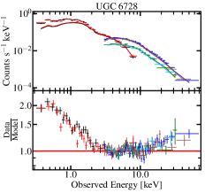
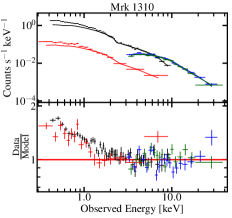
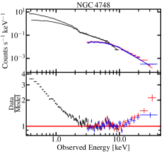
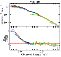
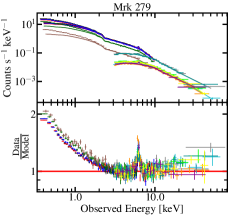
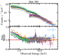
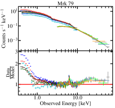
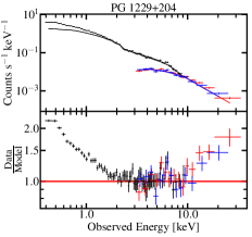
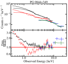
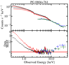
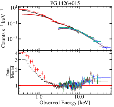
Figure 15: The top panels show the XMM-Newton EPIC and NuSTAR FPM spectral data fitted by the Galactic absorption corrected power-law model (TBabs$*$zpowerlw) in the range 3$-$5 keV and 7$-$10 keV and then extrapolated over the complete energy range for each source. The bottom panel is the corresponding data-to-model ratio. The ratio plot shows soft X-ray excess below around 1$-$2 keV and Fe K emission in the 6$-$7 keV range for each source, along with a hard X-ray excess in the 15$-$30 keV range for some sources. The spectra are re-binned to visualize and demonstrate the shape of the residuals more clearly.

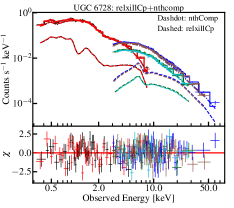
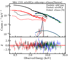
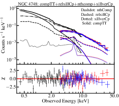
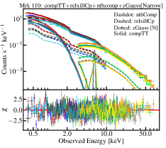
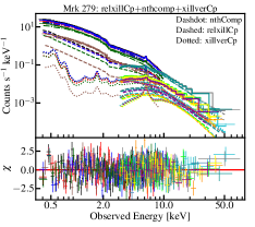
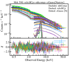
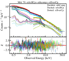
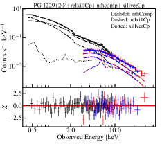
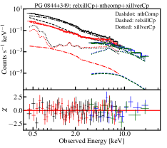
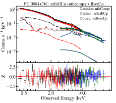
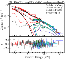
Figure 16: The XMM-Newton/EPIC, NuSTAR/FPMA, and FPMB count spectra with the best-fit models and residuals as a function of energy. Five sets of best-fit models have been obtained for the sample. Whenever the Compton hump is undetected or weak, the narrow 6.4 keV Fe K_α line is modeled by a narrow Gaussian (zGauss[Narrow]) instead of xillverCp. The spectra are binned up only for plotting purposes.

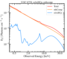
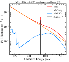
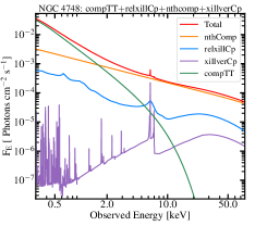
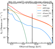
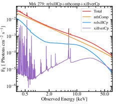
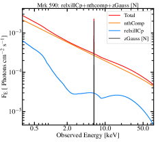
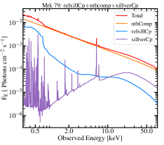
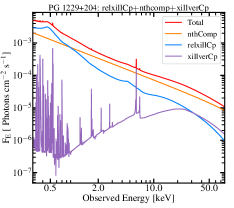
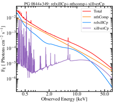
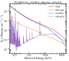
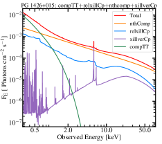
Figure 17: The best-fit spectral energy flux model (in red) with various model components for each source in the sample. The orange, blue, purple, black, and green solid lines represent the primary coronal emission, relativistic disk reflection, distant reflection, narrow Gaussian line, and warm coronal emission, respectively.

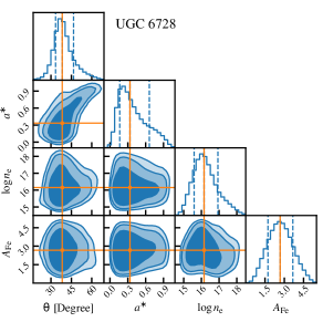
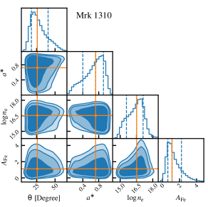
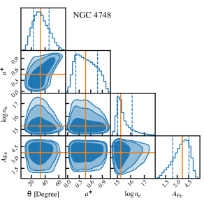
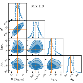
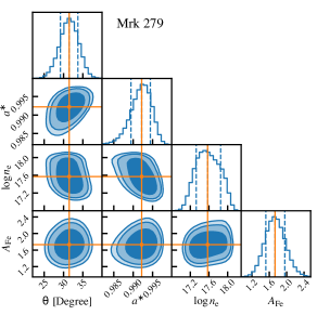
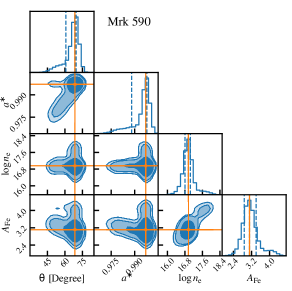
Figure 18: Corner plots for black hole spin, disk density, iron abundance, and disk inclination angle. The on-diagonal histograms demonstrate the MCMC posterior parameter distributions. The median and 68.3% confidence regions are shown in vertical lines. The off-diagonal two-dimensional projections show MCMC contour plots for each pair of parameters. The dark, medium, and light blue areas represent 68.3%, 90%, and 95% confidence levels, respectively, with square symbols indicating parameter medians.

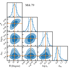
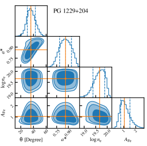
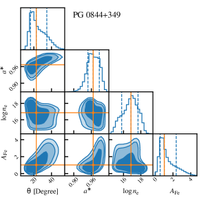
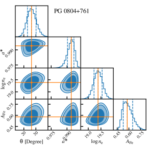
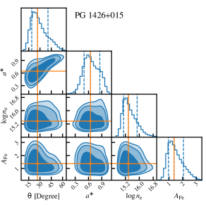
Figure 19: Same as the Figure A4.

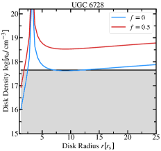
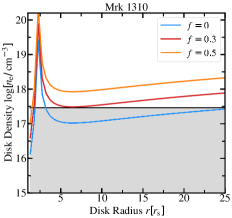
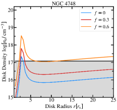
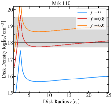
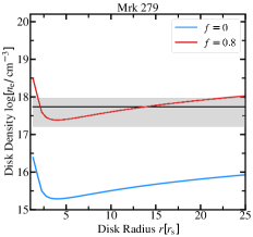
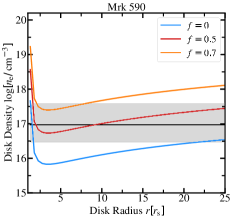
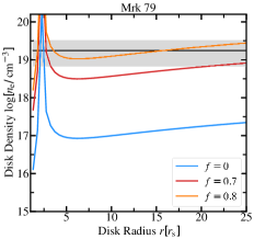
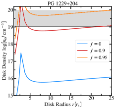
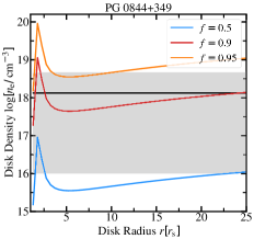
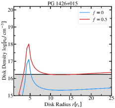
Figure 20: Electron density $\left(\log[n_{\rm e}/{\rm cm^{-3}}]\right)$ of the accretion disk as a function of disk radius ($r$) calculated at different values of disk-to-corona power transfer fraction ($f$) for each source. The black solid line and grey shaded area represent the best-fit $\log n_{e}$ and associated 90% confidence interval, respectively.

References

- Akaike (1974) Akaike, H. 1974, IEEE Transactions on Automatic Control, 19, 716
- Akylas & Georgantopoulos (2021) Akylas, A., & Georgantopoulos, I. 2021, A&A, 655, A60, doi: 10.1051/0004-6361/202141186
- Antonucci (1993) Antonucci, R. 1993, ARA&A, 31, 473, doi: 10.1146/annurev.aa.31.090193.002353
- Arnaud (1996) Arnaud, K. A. 1996, in Astronomical Society of the Pacific Conference Series, Vol. 101, Astronomical Data Analysis Software and Systems V, ed. G. H. Jacoby & J. Barnes, 17
- Arnaud et al. (1985) Arnaud, K. A., Branduardi-Raymont, G., Culhane, J. L., et al. 1985, MNRAS, 217, 105, doi: 10.1093/mnras/217.1.105
- Bambi et al. (2021) Bambi, C., Brenneman, L. W., Dauser, T., et al. 2021, Space Sci. Rev., 217, 65, doi: 10.1007/s11214-021-00841-8
- Bardeen et al. (1972) Bardeen, J. M., Press, W. H., & Teukolsky, S. A. 1972, ApJ, 178, 347, doi: 10.1086/151796
- Barkana & Loeb (2001) Barkana, R., & Loeb, A. 2001, Phys. Rep., 349, 125, doi: 10.1016/S0370-1573(01)00019-9
- Batiste et al. (2017) Batiste, M., Bentz, M. C., Raimundo, S. I., Vestergaard, M., & Onken, C. A. 2017, ApJ, 838, L10, doi: 10.3847/2041-8213/aa6571
- Bentz & Katz (2015) Bentz, M. C., & Katz, S. 2015, PASP, 127, 67, doi: 10.1086/679601
- Berti & Volonteri (2008) Berti, E., & Volonteri, M. 2008, ApJ, 684, 822, doi: 10.1086/590379
- Blackburn (1995) Blackburn, J. K. 1995, in Astronomical Society of the Pacific Conference Series, Vol. 77, Astronomical Data Analysis Software and Systems IV, ed. R. A. Shaw, H. E. Payne, & J. J. E. Hayes, 367
- Brenneman & Reynolds (2006) Brenneman, L. W., & Reynolds, C. S. 2006, ApJ, 652, 1028, doi: 10.1086/508146
- Cappelluti et al. (2024) Cappelluti, N., Foord, A., Marchesi, S., et al. 2024, Universe, 10, 276, doi: 10.3390/universe10070276
- Cappi et al. (2006) Cappi, M., Panessa, F., Bassani, L., et al. 2006, A&A, 446, 459, doi: 10.1051/0004-6361:20053893
- Cash (1979) Cash, W. 1979, ApJ, 228, 939, doi: 10.1086/156922
- Chalise et al. (2022) Chalise, S., Lohfink, A. M., Chauhan, J., et al. 2022, MNRAS, 517, 4788, doi: 10.1093/mnras/stac2953
- Combes et al. (2019) Combes, F., García-Burillo, S., Audibert, A., et al. 2019, A&A, 623, A79, doi: 10.1051/0004-6361/201834560
- Cruise et al. (2025) Cruise, M., Guainazzi, M., Aird, J., et al. 2025, arXiv e-prints, arXiv:2501.03100, doi: 10.48550/arXiv.2501.03100
- Crummy et al. (2006) Crummy, J., Fabian, A. C., Gallo, L., & Ross, R. R. 2006, MNRAS, 365, 1067, doi: 10.1111/j.1365-2966.2005.09844.x
- Dauser et al. (2014) Dauser, T., García, J., Parker, M. L., Fabian, A. C., & Wilms, J. 2014, Monthly Notices of the Royal Astronomical Society: Letters, 444, L100, doi: 10.1093/mnrasl/slu125
- Dauser et al. (2012) Dauser, T., Svoboda, J., Schartel, N., et al. 2012, MNRAS, 422, 1914, doi: 10.1111/j.1365-2966.2011.20356.x
- Di Matteo et al. (2023) Di Matteo, T., Ni, Y., Chen, N., et al. 2023, MNRAS, 525, 1479, doi: 10.1093/mnras/stad2198
- Di Matteo et al. (2005) Di Matteo, T., Springel, V., & Hernquist, L. 2005, Nature, 433, 604, doi: 10.1038/nature03335
- Done et al. (2012) Done, C., Davis, S. W., Jin, C., Blaes, O., & Ward, M. 2012, MNRAS, 420, 1848, doi: 10.1111/j.1365-2966.2011.19779.x
- Elvis et al. (1994) Elvis, M., Wilkes, B. J., McDowell, J. C., et al. 1994, ApJS, 95, 1, doi: 10.1086/192093
- Fabian (1994) Fabian, A. C. 1994, ApJS, 92, 555, doi: 10.1086/192015
- Fabian (2012) —. 2012, ARA&A, 50, 455, doi: 10.1146/annurev-astro-081811-125521
- Fabian et al. (2002) Fabian, A. C., Ballantyne, D. R., Merloni, A., et al. 2002, MNRAS, 331, L35, doi: 10.1046/j.1365-8711.2002.05419.x
- Fabian et al. (2000) Fabian, A. C., Iwasawa, K., Reynolds, C. S., & Young, A. J. 2000, PASP, 112, 1145, doi: 10.1086/316610
- Fabian et al. (2015) Fabian, A. C., Lohfink, A., Kara, E., et al. 2015, MNRAS, 451, 4375, doi: 10.1093/mnras/stv1218
- Fabian et al. (1989) Fabian, A. C., Rees, M. J., Stella, L., & White, N. E. 1989, MNRAS, 238, 729, doi: 10.1093/mnras/238.3.729
- Ferrarese & Merritt (2000) Ferrarese, L., & Merritt, D. 2000, ApJ, 539, L9, doi: 10.1086/312838
- Frank et al. (2002) Frank, J., King, A., & Raine, D. J. 2002, Accretion Power in Astrophysics: Third Edition
- Gabriel et al. (2004) Gabriel, C., Denby, M., Fyfe, D. J., et al. 2004, in Astronomical Society of the Pacific Conference Series, Vol. 314, Astronomical Data Analysis Software and Systems (ADASS) XIII, ed. F. Ochsenbein, M. G. Allen, & D. Egret, 759
- García et al. (2013) García, J., Dauser, T., Reynolds, C. S., et al. 2013, ApJ, 768, 146, doi: 10.1088/0004-637X/768/2/146
- García & Kallman (2010) García, J., & Kallman, T. R. 2010, ApJ, 718, 695, doi: 10.1088/0004-637X/718/2/695
- García et al. (2014) García, J., Dauser, T., Lohfink, A., et al. 2014, ApJ, 782, 76, doi: 10.1088/0004-637X/782/2/76
- García et al. (2016) García, J. A., Fabian, A. C., Kallman, T. R., et al. 2016, MNRAS, 462, 751, doi: 10.1093/mnras/stw1696
- García et al. (2019) García, J. A., Kara, E., Walton, D., et al. 2019, ApJ, 871, 88, doi: 10.3847/1538-4357/aaf739
- George & Fabian (1991) George, I. M., & Fabian, A. C. 1991, MNRAS, 249, 352, doi: 10.1093/mnras/249.2.352
- Gierliński & Done (2004) Gierliński, M., & Done, C. 2004, MNRAS, 349, L7, doi: 10.1111/j.1365-2966.2004.07687.x
- Goodman & Weare (2010) Goodman, J., & Weare, J. 2010, Communications in Applied Mathematics and Computational Science, 5, 65, doi: 10.2140/camcos.2010.5.65
- Gültekin et al. (2009) Gültekin, K., Richstone, D. O., Gebhardt, K., et al. 2009, ApJ, 698, 198, doi: 10.1088/0004-637X/698/1/198
- Gurzadian & Ozernoi (1979) Gurzadian, V. G., & Ozernoi, L. M. 1979, Nature, 280, 214, doi: 10.1038/280214a0
- Haardt & Maraschi (1993) Haardt, F., & Maraschi, L. 1993, ApJ, 413, 507, doi: 10.1086/173020
- Harikane et al. (2023) Harikane, Y., Zhang, Y., Nakajima, K., et al. 2023, ApJ, 959, 39, doi: 10.3847/1538-4357/ad029e
- Harrison et al. (2013) Harrison, F. A., Craig, W. W., Christensen, F. E., et al. 2013, ApJ, 770, 103, doi: 10.1088/0004-637X/770/2/103
- HEASARC (2014) HEASARC. 2014, HEAsoft: Unified Release of FTOOLS and XANADU, Astrophysics Source Code Library, record ascl:1408.004
- Heckman & Best (2014) Heckman, T. M., & Best, P. N. 2014, ARA&A, 52, 589, doi: 10.1146/annurev-astro-081913-035722
- Heyl et al. (2020) Heyl, J., Caiazzo, I., Gallagher, S., Hoffman, K., & Safi-Harb, S. 2020, in Society of Photo-Optical Instrumentation Engineers (SPIE) Conference Series, Vol. 11444, Space Telescopes and Instrumentation 2020: Ultraviolet to Gamma Ray, ed. J.-W. A. den Herder, S. Nikzad, & K. Nakazawa, 114442A, doi: 10.1117/12.2562625
- Hopkins & Elvis (2010) Hopkins, P. F., & Elvis, M. 2010, MNRAS, 401, 7, doi: 10.1111/j.1365-2966.2009.15643.x
- Jansen et al. (2001) Jansen, F., Lumb, D., Altieri, B., et al. 2001, A&A, 365, L1, doi: 10.1051/0004-6361:20000036
- Jeffreys (1961) Jeffreys, H. 1961, Theory of probability, Oxford University Press, London
- Jiang et al. (2019a) Jiang, J., Fabian, A. C., Dauser, T., et al. 2019a, MNRAS, 489, 3436, doi: 10.1093/mnras/stz2326
- Jiang et al. (2019b) Jiang, Y.-F., Blaes, O., Stone, J. M., & Davis, S. W. 2019b, ApJ, 885, 144, doi: 10.3847/1538-4357/ab4a00
- Kaastra & Bleeker (2016) Kaastra, J. S., & Bleeker, J. A. M. 2016, A&A, 587, A151, doi: 10.1051/0004-6361/201527395
- Kang & Wang (2022) Kang, J.-L., & Wang, J.-X. 2022, ApJ, 929, 141, doi: 10.3847/1538-4357/ac5d49
- Kass & Raftery (1995) Kass, R. E., & Raftery, A. E. 1995, Journal of the American Statistical Association, 90, 773. http://www.jstor.org/stable/2291091
- Kelly (2007) Kelly, B. C. 2007, ApJ, 665, 1489, doi: 10.1086/519947
- Kormendy & Ho (2013) Kormendy, J., & Ho, L. C. 2013, ARA&A, 51, 511, doi: 10.1146/annurev-astro-082708-101811
- Lynden-Bell (1969) Lynden-Bell, D. 1969, Nature, 223, 690, doi: 10.1038/223690a0
- Mallick & Dewangan (2018) Mallick, L., & Dewangan, G. C. 2018, ApJ, 863, 178, doi: 10.3847/1538-4357/aad193
- Mallick et al. (2017) Mallick, L., Dewangan, G. C., McHardy, I. M., & Pahari, M. 2017, MNRAS, 472, 174, doi: 10.1093/mnras/stx1960
- Mallick et al. (2021) Mallick, L., Wilkins, D. R., Alston, W. N., et al. 2021, MNRAS, 503, 3775, doi: 10.1093/mnras/stab627
- Mallick et al. (2018) Mallick, L., Alston, W. N., Parker, M. L., et al. 2018, MNRAS, 479, 615, doi: 10.1093/mnras/sty1487
- Mallick et al. (2022) Mallick, L., Fabian, A. C., García, J. A., et al. 2022, MNRAS, 513, 4361, doi: 10.1093/mnras/stac990
- Matt et al. (2014) Matt, G., Marinucci, A., Guainazzi, M., et al. 2014, MNRAS, 439, 3016, doi: 10.1093/mnras/stu159
- NASA/IPAC Extragalactic Database (2019) (NED) NASA/IPAC Extragalactic Database (NED). 2019, NASA/IPAC Extragalactic Database (NED), IPAC, doi: 10.26132/NED1
- Netzer (2015) Netzer, H. 2015, ARA&A, 53, 365, doi: 10.1146/annurev-astro-082214-122302
- Pacucci & Loeb (2020) Pacucci, F., & Loeb, A. 2020, ApJ, 895, 95, doi: 10.3847/1538-4357/ab886e
- Pacucci & Loeb (2022) —. 2022, MNRAS, 509, 1885, doi: 10.1093/mnras/stab3071
- Pacucci & Narayan (2024) Pacucci, F., & Narayan, R. 2024, ApJ, 976, 96, doi: 10.3847/1538-4357/ad84f7
- Page & Thorne (1974) Page, D. N., & Thorne, K. S. 1974, ApJ, 191, 499, doi: 10.1086/152990
- Parker et al. (2017) Parker, M. L., Pinto, C., Fabian, A. C., et al. 2017, Nature, 543, 83, doi: 10.1038/nature21385
- Petrucci et al. (2018) Petrucci, P. O., Ursini, F., De Rosa, A., et al. 2018, A&A, 611, A59, doi: 10.1051/0004-6361/201731580
- Petrucci et al. (2001) Petrucci, P. O., Haardt, F., Maraschi, L., et al. 2001, ApJ, 556, 716, doi: 10.1086/321629
- Pier & Krolik (1993) Pier, E. A., & Krolik, J. H. 1993, ApJ, 418, 673, doi: 10.1086/173427
- Pinto et al. (2018) Pinto, C., Alston, W., Parker, M. L., et al. 2018, MNRAS, 476, 1021, doi: 10.1093/mnras/sty231
- Porquet et al. (2024) Porquet, D., Hagen, S., Grosso, N., et al. 2024, A&A, 681, A40, doi: 10.1051/0004-6361/202347202
- Porquet et al. (2021) Porquet, D., Reeves, J. N., Grosso, N., Braito, V., & Lobban, A. 2021, A&A, 654, A89, doi: 10.1051/0004-6361/202141577
- Porquet et al. (2018) Porquet, D., Reeves, J. N., Matt, G., et al. 2018, A&A, 609, A42, doi: 10.1051/0004-6361/201731290
- Raimundo et al. (2012) Raimundo, S. I., Fabian, A. C., Vasudevan, R. V., Gandhi, P., & Wu, J. 2012, MNRAS, 419, 2529, doi: 10.1111/j.1365-2966.2011.19904.x
- Rees (1984) Rees, M. J. 1984, ARA&A, 22, 471, doi: 10.1146/annurev.aa.22.090184.002351
- Reines et al. (2013) Reines, A. E., Greene, J. E., & Geha, M. 2013, ApJ, 775, 116, doi: 10.1088/0004-637X/775/2/116
- Reynolds (2021) Reynolds, C. S. 2021, ARA&A, 59, 117, doi: 10.1146/annurev-astro-112420-035022
- Reynolds et al. (2023) Reynolds, C. S., Kara, E. A., Mushotzky, R. F., et al. 2023, in Society of Photo-Optical Instrumentation Engineers (SPIE) Conference Series, Vol. 12678, UV, X-Ray, and Gamma-Ray Space Instrumentation for Astronomy XXIII, ed. O. H. Siegmund & K. Hoadley, 126781E, doi: 10.1117/12.2677468
- Ricci et al. (2017) Ricci, C., Trakhtenbrot, B., Koss, M. J., et al. 2017, ApJS, 233, 17, doi: 10.3847/1538-4365/aa96ad
- Ross & Fabian (2005) Ross, R. R., & Fabian, A. C. 2005, MNRAS, 358, 211, doi: 10.1111/j.1365-2966.2005.08797.x
- Ross & Fabian (2007) —. 2007, MNRAS, 381, 1697, doi: 10.1111/j.1365-2966.2007.12339.x
- Salvesen et al. (2016) Salvesen, G., Simon, J. B., Armitage, P. J., & Begelman, M. C. 2016, MNRAS, 457, 857, doi: 10.1093/mnras/stw029
- Shakura & Sunyaev (1973) Shakura, N. I., & Sunyaev, R. A. 1973, A&A, 24, 337
- Silk & Rees (1998) Silk, J., & Rees, M. J. 1998, A&A, 331, L1, doi: 10.48550/arXiv.astro-ph/9801013
- Singh et al. (1985) Singh, K. P., Garmire, G. P., & Nousek, J. 1985, ApJ, 297, 633, doi: 10.1086/163560
- Spiegelhalter et al. (2002) Spiegelhalter, D. J., Best, N. G., Carlin, B. P., & Van Der Linde, A. 2002, Journal of the Royal Statistical Society: Series B (Statistical Methodology), 64, 583, doi: 10.1111/1467-9868.00353
- Sunyaev & Titarchuk (1980) Sunyaev, R. A., & Titarchuk, L. G. 1980, A&A, 86, 121
- Svensson & Zdziarski (1994) Svensson, R., & Zdziarski, A. A. 1994, ApJ, 436, 599, doi: 10.1086/174934
- Tombesi et al. (2011) Tombesi, F., Sambruna, R. M., Reeves, J. N., Reynolds, C. S., & Braito, V. 2011, MNRAS, 418, L89, doi: 10.1111/j.1745-3933.2011.01149.x
- Tortosa et al. (2018) Tortosa, A., Bianchi, S., Marinucci, A., Matt, G., & Petrucci, P. O. 2018, A&A, 614, A37, doi: 10.1051/0004-6361/201732382
- Van Rossum & Drake (2009) Van Rossum, G., & Drake, F. L. 2009, Python 3 Reference Manual (Scotts Valley, CA: CreateSpace)
- Vasudevan & Fabian (2007) Vasudevan, R. V., & Fabian, A. C. 2007, MNRAS, 381, 1235, doi: 10.1111/j.1365-2966.2007.12328.x
- Vasudevan et al. (2016) Vasudevan, R. V., Fabian, A. C., Reynolds, C. S., et al. 2016, MNRAS, 458, 2012, doi: 10.1093/mnras/stw363
- Verner et al. (1996) Verner, D. A., Ferland, G. J., Korista, K. T., & Yakovlev, D. G. 1996, ApJ, 465, 487, doi: 10.1086/177435
- Volonteri et al. (2005) Volonteri, M., Madau, P., Quataert, E., & Rees, M. J. 2005, ApJ, 620, 69, doi: 10.1086/426858
- Volonteri et al. (2013) Volonteri, M., Sikora, M., Lasota, J. P., & Merloni, A. 2013, ApJ, 775, 94, doi: 10.1088/0004-637X/775/2/94
- Wilkins et al. (2014) Wilkins, D. R., Kara, E., Fabian, A. C., & Gallo, L. C. 2014, MNRAS, 443, 2746, doi: 10.1093/mnras/stu1273
- Willingale et al. (2013) Willingale, R., Starling, R. L. C., Beardmore, A. P., Tanvir, N. R., & O’Brien, P. T. 2013, MNRAS, 431, 394, doi: 10.1093/mnras/stt175
- Wilms et al. (2000) Wilms, J., Allen, A., & McCray, R. 2000, ApJ, 542, 914, doi: 10.1086/317016
- Zdziarski et al. (1996) Zdziarski, A. A., Johnson, W. N., & Magdziarz, P. 1996, MNRAS, 283, 193, doi: 10.1093/mnras/283.1.193
- Zhao et al. (2021) Zhao, X., Marchesi, S., Ajello, M., et al. 2021, A&A, 650, A57, doi: 10.1051/0004-6361/202140297