Learning-Enhanced Safeguard Control for High-Relative-Degree Systems: Robust Optimization under Disturbances and Faults

Abstract

Merely pursuing performance may adversely affect the safety, while a conservative policy for safe exploration will degrade the performance. How to balance the safety and performance in learning-based control problems is an interesting yet challenging issue. This paper aims to enhance system performance with safety guarantee in solving the reinforcement learning (RL)-based optimal control problems of nonlinear systems subject to high-relative-degree state constraints and unknown time-varying disturbance/actuator faults. First, to combine control barrier functions (CBFs) with RL, a new type of CBFs, termed high-order reciprocal control barrier function (HO-RCBF) is proposed to deal with high-relative-degree constraints during the learning process. Then, the concept of gradient similarity is proposed to quantify the relationship between the gradient of safety and the gradient of performance. Finally, gradient manipulation and adaptive mechanisms are introduced in the safe RL framework to enhance the performance with a safety guarantee. Two simulation examples illustrate that the proposed safe RL framework can address high-relative-degree constraint, enhance safety robustness and improve system performance.

Safety guarantee, high-order reciprocal control barrier function, reinforcement learning

1 Introduction

In practice, safety, optimality and stability are three important design objectives for control systems, especially safety-critical and resource-constrained systems [1, 2]. As an effective approach to simultaneously consider stability, optimality and safety, safe optimal control has attracted increasing attention in the control community in the past few years, which aims to stabilize dynamical systems while minimizing a user-defined cost function and adhering to certain safety constraints. It has been successfully applied in various practical scenarios, such as autonomous driving [3] and trajectory optimization [4].

So far, many approaches, such as model predictive control and safety filter, to name a few [5], have been investigated to address safe optimal control problems. However, these approaches require accurate system information to project the optimal controller into the safe input set, and thus cannot rigorously guarantee safety in the presence of disturbances. As an effective tool for designing optimal controllers for uncertain systems, reinforcement learning (RL) has been studied for addressing safe optimal control problems by using some technical strategies, such as external knowledge [6], reachability analysis [7], and worst-case criterion [8].

Despite their success in practical applications, these approaches encounter a serious challenge of computational cost, especially for high-dimensional systems. To reduce the computational burden, the concept of control barrier function (CBF) was introduced in [9] as a safety constraint to certify the forward invariance of a safety set. Two notions of CBF are commonly utilized i.e., reciprocal CBF (RCBF) and zeroing CBF (ZCBF). The former goes to infinity when approaching the boundary of the safety set, while the latter vanishes.

Recently, CBF has been integrated into RL techniques to address safe, optimal control problems. The approach from [10] utilizes the barrier transformation technique to map a constrained system to an unconstrained one, allowing standard RL techniques to be applied directly. Unfortunately, these techniques are restricted to box safety constraints and cannot adequately address complex safety constraints, such as ellipsoidal and cone safety constraints [11, 12], which are frequently encountered in robotic control. Similar to the penalty method (see Chapter 2.1.1 in [13]), a barrier function-based penalty term is incorporated into the cost function in [14], taking into account both optimality and safety during the learning process. However, as argued in [15], the effectiveness of the CBF-based penalty method strongly depends on the proper design of the cost function, and an improper cost function may lead to undesirable learning results. It is also worth noting that approaches [14, 10], where safety and optimality are tightly coupled, may violate the safety constraints during the learning process.

Different from the approaches [14, 10], a recent work[16] introduces a safeguarding-based RL method that emphasizes learning a performance-driven policy while guaranteeing safety through an augmented safeguarding policy. In other words, this method simplifies the learning target by decoupling the safety objective from the learning process using a safeguarding policy. This allows the method to focus solely on optimizing performance, thus reducing the computational cost. Furthermore, as noted by [17], the safeguarding-based RL method essentially replaces the real-time calculation of the Lagrange multiplier with a constant gain, which also contributes to the reduction of computational burden. This method has been successfully applied in multi-quadrator systems to address safe human-swarm interaction problems [18]. Although this safeguarding-based RL approach can significantly reduce the computational burden, it is limited to specific safety scenarios, such as safety constraints with relative degree one, and it also leads to a more conservative solution. Using a high-order ZCBF-based safety filter to project the unsafe control policy into the set of safe policies, the RL approach from [19] can address high-relative-degree constraints, where the Lagrange multiplier is instantly calculated. Hence, the computational cost of the approach from [19] is more expensive than the approach from [16], and safety may be destroyed by disturbance/fault, which will be shown in the simulation section. The limitations discussed above motivate our in-depth investigation into safeguarding-based RL approaches. Specifically, on the basis of [16], we extend the safeguarding-based RL to address optimal control problems subject to high-relative-degree constraints. Also, given that objectives of stability/optimality and safety may be conflicting, our objective is to provide a control system that compromises between safety concerns and performance requirements. Furthermore, we explore the robustness of safeguarding-based RL to unknown disturbance/actuator fault, which is not discussed in [16].

In this paper, we propose an adaptive safeguarding-based RL framework for optimal control problems in the presence of unknown disturbance/fault and high-relative-degree safety constraints. First, inspired by the high-order ZCBFs (HO-ZCBFs) defined in [20], we introduce a new type of CBFs, termed high-order RCBFs (HO-RCBFs), which are capable of evaluating the safety of systems subject to high-relative-degree constraints. The key difference between HO-RCBFs and HO-ZCBFs is that HO-RCBFs require large power to push the system trajectory away from the boundary of the safety set, while HO-ZCBFs vanish as it approaches the boundary of the safety set. This property facilitates the integration of HO-RCBFs with RL to address constrained optimal control problems. Second, we extend the safeguarding controller from [16] to a high-order version to handle high-relative-degree safety constraints and rigorously analyze its robustness to unknown disturbance/fault. Most importantly, our approach formally achieves a weighted balance between safety and performance with theoretically guaranteed safety. This problem, which encourages user-defined greedy exploration, has been recognized as a significant challenge in safe RL [21]. It is worth noting that theoretically guaranteed safe control policy for continuous-time systems might violate the safety when the controller is practically implemented in a discrete-time manner, especially when the control frequency is not sufficiently high (see Example 3.11 in Section 3 for details). This is why we need to achieve a weighted balance between safety and performance. By doing so, the performance of the system can be reduced flexibly according to practical safety requirements. And, in contrast to existing works on safeguarding-based RL, asymptotic stability of the system can be guaranteed.

Notations: Matrix $P>0$ means $P$ is positive definite. Both the Euclidean norm of a vector and the Frobenius norm of a matrix are denoted by $\lVert\cdot\rVert$, respectively. The maximum and minimum eigenvalues of a matrix are denoted by $\bar{\sigma}(\cdot)$ and $\underline{\sigma}(\cdot)$, respectively. For a time-varying bounded signal $d(t)$, we define $\lVert d\rVert_{\infty}=\sup_{t\in\mathbb{R}}\lVert d(t)\rVert$. The inner product of any two vectors $y_{1}$ and $y_{2}$ is denoted by $\langle y_{1},y_{2}\rangle$. For a continuously differentiable function $Y(c)$, we define $\nabla_{c}Y=\partial Y/\partial c$. Given any compact set $\mathcal{V}\subset\mathbb{R}^{q}$ and a continuous mapping $p:\mathcal{V}\rightarrow\mathbb{R}^{Q}$, $\overline{\lVert p(v)\rVert}_{\mathcal{V}}=\mathop{\rm{sup}}_{v\in\mathcal{V}}\lVert p(v)\rVert$.

2 Problem formulation

Consider a continuous-time nonlinear control affine system

$$\dot{x}=f\left(x\right)+g\left(x\right)(u+u^{f})$$ (1)

and its nominal system

$$\dot{x}=f\left(x\right)+g\left(x\right)u$$ (2)

where $x\in\mathbb{R}^{n}$ and $u\in\mathbb{R}^{p}$ are the state vector and the input vector of the system, respectively; $u^{f}\in\mathbb{R}^{p}$ represents the unknown actuator fault and/or matched disturbance. The drift dynamics $f:\mathbb{R}^{n}\rightarrow\mathbb{R}^{n}$ and the control dynamics $g:\mathbb{R}^{n}\rightarrow\mathbb{R}^{n\times p}$ are locally Lipschitz. It is assumed $f(0)=0$ and the system is stabilizable. Given a stabilizing control policy $u(t)=k(x,t)$ such that $k(0,t)=0$, $f(x)+g(x)k(x,t)$ is locally Lipschitz in $x$ and piecewise continuous in $t$, for any initial state $x_{0}$ at $0$, there always exists a solution of the system satisfying

$$\dot{x}=f\left(x\right)+g\left(x\right)k(x,t), x(0)=x_{0}.$$

Assumption 1

The actuator fault/matched disturbance are bounded, continuously differentiable signals with bounded time derivative, i.e.,

$$u^{f}\in\mathcal{U}^{f}:=\{u^{f}\in\mathbb{R}^{p}\;|\;\lVert u^{f}\rVert_{\infty}\leq\eta_{1},\lVert\dot{u}^{f}\rVert_{\infty}\leq\eta_{2}\},$$

where $\eta_{1}$ and $\eta_{2}$ are unknown positive constants.

Remark 1

In practice, it is reasonable to make Assumption 1 on $u^{f}$ [22]. As an actuator fault, $u^{f}$ can represent force biases caused by motors in unmanned aerial vehicles [23], actuator bias of distributed generators in microgrids [24], and so on. In addition, $u^{f}$ can represent a matched disturbance, which is a common occurrence in several practical applications, such as permanent magnet synchronous motors [25] and unmanned vehicles [26].

2.1 Unconstrained optimal control

To seek an optimal control policy for (3), one way is to solve the following optimal control problem [27]

$$\mathop{\rm{inf}}_{u\in\mathbb{R}^{p}}J(x,u):=\int_{0}^{\infty}\underbrace{x(\tau)^{\top}Qx(\tau)+u(\tau)^{\top}Ru(\tau)}_{l\left(x(\tau),u(\tau)\right)}d\tau,$$ (3)

where $J$ is the user-defined cost function and $Q,R>0$.

To address such an optimal control problem, the optimal value function is defined as

$$V^{*}(x(t))=\mathop{\rm{inf}}\limits_{u\in\mathbb{R}^{p}}\int_{t}^{\infty}l\left(x(\tau),u(\tau)\right)d\tau.$$

and the Hamiltonian function can be obtained by differentiating the optimal value function

$$H(x,\nabla V^{*}(x),u)=\nabla V^{*}(x)^{\top}(f(x)+g(x)u)+l(x,u)$$ (4)

where $\nabla V^{*}(x)=\partial V^{*}(x)/\partial x$ and $V^{*}(0)=0$.

Provided a continuously differentiable $V^{*}(x)$ exists, it is the unique positive definite solution of the Hamilton-Jacobi-Bellman (HJB) equation

$$\mathop{\rm{inf}}\limits_{u\in\mathbb{R}^{p}}H(x,\nabla V^{*}(x),u)=0.$$ (5)

By applying the optimal condition $\partial H/\partial u=0$, the optimal control policy can be derived as

$$k^{*}(x)=-\frac{1}{2}R^{-1}g(x)^{\top}\nabla V^{*}(x).$$ (6)

2.2 Constrained optimal control

Suppose $x$ is subject to inequality constraints and can be mathematically formulated as $x\in\mathscr{C}\subset\mathbb{R}^{n}$. The set $\mathscr{C}$ is nonempty with no isolated point and it has the following form

$$\mathscr{C}=\{x\in\mathbb{R}^{n}\;|\;h(x)\geq 0\}$$

$$\mathscr{C}^{S}=\{x\in\mathbb{R}^{n}\;|\;h(x)=0\}$$

$$\operatorname{Int}(\mathscr{C})=\{x\in\mathbb{R}^{n}\;|\;h(x)>0\}$$

where $h:\mathbb{R}^{n}\rightarrow\mathbb{R}$ is $m$th-order differentiable. Then, a standard-constrained optimal control problem can be formulated as follows.

Problem 1

Consider the nominal nonlinear system (2) and a safety set $\mathscr{C}\subset\mathbb{R}^{n}$. Find an admissible control policy $u(\cdot)$ to solve the optimal control problem (3) while rendering the set $\mathscr{C}$ forward invariant [28], i.e.,

$$\inf_{u\in\mathbb{R}^{p}}\;\int_{0}^{\infty}l(x(\tau),u(\tau))d\tau$$ (7)

$$\textnormal{s.t.}\qquad x(t)\in\mathscr{C},\;\forall t\geq 0,~x(0)\in\mathscr{C}$$

For (7), the control policy (6) is optimal but generally does not satisfy the constraint. Considering the fact that directly solving (7) is computationally expensive and inefficient, CBFs are applied to provide sub-optimal, but computationally efficient, solutions to constrained optimal control problems. Before presenting CBF-based solution of the constrained control problem, we introduce some basic definitions commonly encountered in safe control methodologies.

Definition 1

[9] (Reciprocal control barrier function): A continuously differentiable function $b:\mathscr{C}\rightarrow\mathbb{R}_{\geq 0}$ is a reciprocal control barrier function (RCBF) with respect to $h(x)$ for the system (2) if there exist class $\mathcal{K}$ functions $\beta_{1},\beta_{2}$ and $\beta_{3}$ such that, for all $x\in\operatorname{Int}(\mathscr{C})$

$$\frac{1}{\beta_{1}(h(x))}\leq b(x) \leq\frac{1}{\beta_{2}(h(x))}$$

$$\mathop{\rm{inf}}\limits_{u\in\mathbb{R}^{p}}\{\mathcal{L}_{f}b(x)+\mathcal{L}_{g}b(x)u\} \leq\beta_{3}(h(x))$$

where $\nabla b(x)=\partial b(x)/\partial x$, $\mathcal{L}_{f}b(x)=\nabla b(x)^{\top}f(x)$ and $\mathcal{L}_{g}b(x)=\nabla b(x)^{\top}g(x)$ are Lie derivatives of $b(x)$ along $f(x)$ and $g(x)$, respectively.

Definition 2

(Relative degree): Given a safety set $\mathscr{C}$. An $r_{th}$-order differentiable function $h:\mathbb{R}^{n}\rightarrow\mathbb{R}$ is said to have a relative degree of $m\leq r$ with respect to (1), if $\forall x\in\mathscr{C}^{S}$, there exists a neighborhood of $x$ such that in this neighborhood

$$\lVert\mathcal{L}_{g}\mathcal{L}_{f}^{m-1}h(x)\rVert\neq 0\ \ \textnormal{and}\ \ \lVert\mathcal{L}_{g}\mathcal{L}_{f}^{k}h(x)\rVert=0,$$

$\forall k=0,1,\dots,m-2$.

Many existing works combine CBFs and RL to solve optimal control problems while guaranteeing the safety of (2). In [16], a safeguarding policy $u_{s}(x)$ is introduced to learn the unconstrained optimal control policy $k^{*}(x)$ safely, and the controller becomes

$$u(x)=\underbrace{-K_{s}R^{-1}\mathcal{L}_{g}b(x)^{\top}}_{u^{s}(x)}+k^{*}(x),$$

where $R>0$ is the same weight in (3) and $K_{s}>0$ is a user-defined safeguarding gain. For the case of $m=1$, $u^{s}(x)$ can keep the state trajectory of system (2) with $k^{*}(x)$ staying in $\operatorname{Int}(\mathscr{C})$ for any $x_{0}\in\operatorname{Int}(\mathscr{C})$. The disturbance considered in this problem can be generalized to mismatched disturbance.

However, provided that $h(x)$ has relative degree $m>1$ with respect to (2), the safeguarding controller cannot be utilized to guarantee safety, due to the absence of the control terms.

It is worth noting that many practical applications have high-relative-degree constraints, such as traffic merging [29], adaptive cruise control [30] and motion planning [31]. However, effective safeguarding policies with the ability to address high-relative-degree constraints has not been satisfactorily investigated to date. In the next section, we shall extend the safeguarding control policy to address high-relative-degree constraints.

3 Adaptive high-order safeguarding control

3.1 High-order RCBF

We define a series of functions as

$$\psi_{i}(x)=\dot{\psi}_{i-1}(x)+\alpha_{i}\left(\psi_{i-1}(x)\right), i\in\{1,2,\cdots,m\}$$ (8)

where $\psi_{0}(x)=h(x)$ and $\alpha_{1}$, $\alpha_{2}$, $\cdots$, $\alpha_{m-1}$ are sufficiently smooth extended class $\mathcal{K}$ functions such that $\psi_{i}(x_{0})>0$ for $1,2,\cdots,m-1$. Then we define a series of sets $\mathscr{C}_{i}$ of the form

$$\mathscr{C}_{i}=\{x\in\mathbb{R}^{n}\;|\;\psi_{i-1}(x)>0\}, i\in\{1,2,\cdots,m\},$$ (9)

and propose a high-order RCBF (HO-RCBF) defined as follows.

Definition 3

(HO-RCBF): Given a safety set $\mathscr{C}$, let $\psi_{i-1}(x)$ and $\mathscr{C}_{i}$ be defined as (8) and (9) for all $i\in\{1,2,\cdots,m\}$, respectively. A continuously differentiable function $B:\mathscr{C}_{m}\rightarrow\mathbb{R}$ is a HO-RCBF for the nonlinear system (2) if $\forall x_{0}\in\operatorname{Int}(\mathscr{C})$, there exist class $\mathcal{K}$ functions $\gamma_{1}$, $\gamma_{2}$ and $\gamma_{3}$ such that $\forall x\in\bar{\mathscr{C}}:=\bigcap\limits_{i=1}^{m}\mathscr{C}_{i}$,

$$\frac{1}{\gamma_{1}\left(\psi_{m-1}\right)}\leq B(\psi_{m-1}) \leq\frac{1}{\gamma_{2}\left(\psi_{m-1}\right)},$$

$$\mathop{\rm{inf}}\limits_{u\in\mathbb{R}^{p}}\left\{\mathcal{L}_{f}B(\psi_{m-1})+\mathcal{L}_{g}B(\psi_{m-1})u\right\} \leq\gamma_{3}\left(\psi_{m-1}\right),$$ (10)

where the argument $x$ of $\psi_{m-1}$ is omitted for simplicity, and,

$$\nabla B(\psi_{m-1}) =\frac{\partial B(\psi_{m-1})}{\partial\psi_{m-1}},$$

$$\mathcal{L}_{f}B(\psi_{m-1}) =\nabla B(\psi_{m-1})^{\top}\mathcal{L}_{f}\psi_{m-1},$$

$$\mathcal{L}_{g}B(\psi_{m-1}) =\nabla B(\psi_{m-1})^{\top}\mathcal{L}_{g}\psi_{m-1}.$$

When $m=1$, the HO-RCBF is reduced to a RCBF [9]. Given any $x_{0}\in\operatorname{Int}(\mathscr{C})$, one can always find $\mathcal{K}$ functions $\alpha_{i}$ such that $\psi_{i}(x_{0})>0$, $\forall i\in\{1,2,\cdots,m\}$, i.e., $x_{0}\in\bar{\mathscr{C}}$. Since $\bar{\mathscr{C}}\subset\operatorname{Int}(\mathscr{C})$, one can show $x(t)\in\operatorname{Int}(\mathscr{C}),\forall t\geq 0$ if $\bar{\mathscr{C}}$ is forward invariant. In the following Lemma, we illustrate that the existence of a HO-RCBF for (2) implies the existence of a safe policy that renders $\bar{\mathscr{C}}$ forward invariant.

Lemma 1

The set $\bar{\mathscr{C}}$ is forward invariant for system (2) under any Lipschitz continuous control policy $u\in K_{hf}(x)$ if $B(\psi_{m-1})$ is a HO-RCBF candidate, where $K_{hf}(x)=\\ \{u\in\mathbb{R}^{p}\;|\;\mathcal{L}_{f}B(\psi_{m-1})+\mathcal{L}_{g}B(\psi_{m-1})u\leq\gamma_{3}\left(\psi_{m-1}\right)\}.$

Proof 3.1.

From $\psi_{m-1}(x_{0})>0$ and a HO-RCBF candidate $B(\psi_{m-1})$, we have $B(\psi_{m-1})<\infty$ at $x_{0}$ and

$$\dot{B}(\psi_{m-1})\leq\gamma_{3}(\psi_{m-1}).$$

Thus, one has $B(\psi_{m-1})<\infty$ and further $\psi_{m-1}(x)>0$, $\forall t\in[0,\infty)$, which implies $x\in\mathscr{C}_{m}$. Based on the definition (8), $\psi_{m-1}(x)>0$, i.e.,

$$\dot{\psi}_{m-2}(x)+\alpha_{m-1}(\psi_{m-2}(x))>0,$$

implies that $x\in\mathscr{C}_{m-1}$ since $\psi_{m-2}(x_{0})>0$. Iteratively, we have $x\in\mathscr{C}_{1}$ for $\forall t\in[0,\infty)$. Therefore, $x\in\bar{\mathscr{C}}$ for all $t\geq 0$ if $x(0)\in\bar{\mathscr{C}}$. Hence, $\bar{\mathscr{C}}$ is forward invariant.

By Lemma 1, given a constrained optimal control problem with a safe initial state, one can always convert the safety objective to rendering the set $\bar{\mathscr{C}}$ forward invariant by constructing a valid HO-RCBF candidate. Taking disturbance/actuator fault into consideration, and using a HO-RCBF to certify the forward invariance of $\bar{\mathscr{C}}$, we reformulate the constrained optimal control problem as follows.

Problem 3.2.

Consider the nonlinear system (1) subject to unknown actuator bias fault and/or disturbance, and a safety set $\mathscr{C}\subset\mathbb{R}^{n}$ described by a differentiable function $h:\mathbb{R}^{n}\rightarrow\mathbb{R}$ with arbitrary relative degree $m\geq 1$. Given any $x_{0}\in\operatorname{Int}(\mathscr{C})$, define a series of functions $\psi_{i}$ (8) and a series of corresponding sets $\mathscr{C}_{i}$ (9) satisfying $\psi_{i}(x_{0})>0$, $\forall i=1,2,\cdots m$. For

$$\bar{\mathscr{C}}=\mathscr{C}_{1}\cap\cdots\cap\mathscr{C}_{m-1}\cap\mathscr{C}_{m},$$

let $B(\psi_{m-1})$ be a valid HO-RCBF with respect to (1). Find an admissible control policy to solve

$$\inf_{u\in\mathbb{R}^{p}}\;\int_{0}^{\infty}l(x(\tau),u(\tau))d\tau$$

$$\textnormal{s.t.}\quad\mathcal{L}_{f}B(\psi_{m-1})+\mathcal{L}_{g}B(\psi_{m-1})(u+u^{f})\leq\gamma_{3}\left(\psi_{m-1}\right)$$

where $u^{f}$ satisfies Assumption 1.

Before presenting the solution, we make some assumptions.

Assumption 2

Given the system (1) and the safety set $\mathscr{C}$, the following conditions hold:

1. The origin lies in $\operatorname{Int}(\mathscr{C})$, and there exists a neighborhood $N_{l}$ of the origin such that $N_{l}\cap\mathscr{C}^{S}=\emptyset$.

2. There exist positive constants $\bar{g}$ and $\underline{g}$ such that $\underline{g}\leq\lVert g(x)\rVert\leq\bar{g}$ for all $x\in\mathscr{C}_{m}$.

Remark 3.3.

The first condition in Assumption 2 is made for excluding the case where $0\in\mathscr{C}^{S}$, as RCBFs cannot guarantee the safety in this scenario. The second condition guarantees that the control gains are not required to vanish or explode to preserve the safety and stability of the system.

3.2 High-order safeguarding policy

If the optimal value function $V^{*}(x)$ exists, it is the unique positive definite solution of the following problem [15]

$$\mathop{\rm{inf}}\limits_{u\in\mathbb{R}^{p}}\;H(x,\nabla V^{*}(x),u)$$ (11)

$$\textnormal{s.t.}\quad\mathcal{L}_{f}B(\psi_{m-1})+\mathcal{L}_{g}B(\psi_{m-1})(u+u^{f})\leq\gamma_{3}\left(\psi_{m-1}\right),$$

where $H(x,\nabla V^{*}(x),u)$ is the same Hamiltonian function as (4), and $V^{*}(0)=0$. Define the Lagrangian function

$$L(x,\nabla V^{*}(x),u,u^{f},\lambda)= \ H(x,\nabla V^{*}(x),u)+\lambda^{\top}\left(\mathcal{L}_{f}B(\psi_{m-1})\right.$$

$$\left.+\mathcal{L}_{g}B(\psi_{m-1})(u+u^{f})-\gamma_{3}\left(\psi_{m-1}\right)\right)$$

where $\lambda$ is the Lagrange multiplier.

Using the Karush-Kuhn-Tucker (KKT) conditions [32], we have

$$\underbrace{\frac{\partial H}{\partial u}+\left(\mathcal{L}_{g}B(\psi_{m-1})\right)^{\top}\lambda}_{\frac{\partial L}{\partial u}}= \ 0,$$

$$\mathcal{L}_{f}B(\psi_{m-1})+\mathcal{L}_{g}B(\psi_{m-1})(u+u^{f})-\gamma_{3}\left(\psi_{m-1}\right)\leq \ 0,$$

$$\lambda^{\top}\left(\mathcal{L}_{f}B(\psi_{m-1})+\mathcal{L}_{g}B(\psi_{m-1})(u+u^{f})-\gamma_{3}\left(\psi_{m-1}\right)\right)= \ 0,$$

$$\lambda\geq \ 0.$$

Solving the above set of equations/inequalities yields the safe optimal control policy

$$u(x)=\underbrace{-\lambda R^{-1}\mathcal{L}_{g}B(\psi_{m-1})^{T}}_{u^{s}(x)}+k^{*}(x),$$ (12)

and the optimal Lagrange multiplier

$$\lambda=\max\left(\frac{\mathcal{L}_{f}B+\mathcal{L}_{g}B(k^{*}(x)+u^{f})-\gamma_{3}\left(\psi_{m-1}\right)}{\mathcal{L}_{g}BR^{-1}\mathcal{L}_{g}B^{\top}},0\right).$$

Remark 3.4.

It is noted that the controller (12) has some implementation issues. For example, $\lambda$ has to be computed in real-time, which may not work when the control board has a low bandwidth. Computation of $\lambda$ requires accurate information of the disturbance $u^{f}$ which is hard to obtain, if possible. Even if the upper bound of $u^{f}$ is known, the robust form of the HO-CBF will be subject to some conservativeness. It is shown in Section 5 that small uncertainties of the signal $u^{f}$ may lead to an inappropriate value of $\lambda$, which can potentially cause further violations of the safety constraint.

Considering the control policy (12), we replace $\lambda$ with a constant positive safeguarding gain $K_{s}$ to remove the dependency on accurate system information and reduce computational requirements. This yields the proposed high-order safeguarding controller

$$u^{s}=-K_{s}R^{-1}\mathcal{L}_{g}\psi_{m-1}^{T}\nabla\mathcal{B}(x),$$ (13)

where $\nabla\mathcal{B}(x)=\partial\mathcal{B}(x)/\partial\psi_{m-1}$, and $\mathcal{B}(x)$ is an energy function satisfying

$$\inf_{x\in\mathscr{C}_{m}}\mathcal{B}(x)\geq 0,\hskip 17.07182pt\mathcal{B}(0)=0,\hskip 17.07182pt\lim_{x\rightarrow\mathscr{C}_{m}^{S}}\mathcal{B}(x)=\infty,$$ (14)

where $\mathscr{C}_{m}^{S}=\{x\in\mathbb{R}^{n}\;|\;\psi_{m-1}(x)=0\}$. For example,

$$\mathcal{B}(x)=(B(\psi_{m-1}(x))-B(\psi_{m-1}(0)))^{2}.$$

Since $\psi_{m-1}(x)>0$ if $\mathcal{B}(x)<\infty$, the forward invariance of $\mathscr{C}_{m}$ can also be verified by $\mathcal{B}(x)$. Compared with (12), this controller does not need to compute $\lambda$, and requires no information of the disturbance $u^{f}$.

The following result illustrates that $\eqref{e3.1.3}$ always satisfy the CBF conditions as $x$ approaches the boundary of the safety set and renders $\bar{\mathscr{C}}$ forward invariant in the presence of unknown disturbance/actuator fault.

Theorem 1.

Given any $x_{0}\in\operatorname{Int}(\mathscr{C})$, let $\mathscr{C}_{i}$ and $\psi_{i-1}(x)$, $i\in\{1,2,\cdots,m\}$, be defined as (8) and (9) such that $x_{0}\in\bar{\mathscr{C}}$. Under Assumptions 1-2, the high-order safeguarding controller (13) can guarantee the safety of both the nominal system (2) and the system (1) subject to unknown disturbance/actuator fault $u^{f}$, i.e. $x(t)\in\bar{\mathscr{C}}$, $\forall t\geq 0$ and $\forall x_{0}\in\bar{\mathscr{C}}$.

Proof 3.5.

Since $h(x)$ has relative degree $m>1$, one has

$$\lVert\mathcal{L}_{g}\mathcal{L}_{f}^{i-1}h(x)\rVert=0, \forall i\in\{1,2,\cdots,m-1\}.$$

Hence, the actuator fault $u^{f}$ will not cause any construction error in the sequence of sets $\mathscr{C}_{i}$ for $i=\{1,2,\cdots,m\}$, which implies that the HO-RCBF can still be used to guarantee the forward invariance of $\bar{\mathscr{C}}$. The time derivative of $\mathcal{B}(x)$ along the state trajectories is

$$\dot{\mathcal{B}}(x)= \ \nabla\mathcal{B}(x)^{\top}\left(\mathcal{L}_{f}\psi_{m-1}+\mathcal{L}_{g}\psi_{m-1}(u_{s}(x)+u^{f})\right)$$

$$\leq \ \lVert\nabla\mathcal{B}(x)\rVert\left(\lVert\mathcal{L}_{f}\psi_{m-1}\rVert+\lVert\mathcal{L}_{g}\psi_{m-1}\rVert\lVert u^{f}\rVert\right)$$

$$-K_{s}\nabla\mathcal{B}(x)^{\top}\mathcal{L}_{g}\psi_{m-1}R^{-1}\mathcal{L}_{g}\psi_{m-1}^{\top}\nabla\mathcal{B}(x).$$

Since $\lVert u^{f}\rVert_{\infty}\leq\eta_{1}$, $\lVert\mathcal{L}_{g}\psi_{m-1}\rVert\neq 0$ and

$$\mathcal{L}_{g}\psi_{m-1}R^{-1}\mathcal{L}_{g}\psi_{m-1}^{\top}\geq\bar{\sigma}(R)^{-1}\lVert\mathcal{L}_{g}\psi_{m-1}\rVert^{2},$$

we have

$$\dot{\mathcal{B}}(x)\leq\lVert\nabla\mathcal{B}(x)\rVert^{2}\left(\frac{L_{\psi}}{\lVert\nabla\mathcal{B}(x)\rVert}-\frac{K_{s}}{\bar{\sigma}(R)}\lVert\mathcal{L}_{g}\psi_{m-1}\rVert^{2}\right),$$

where $L_{\psi}=\lVert\mathcal{L}_{f}\psi_{m-1}\rVert+\lVert\mathcal{L}_{g}\psi_{m-1}\rVert\eta_{1}$.

Consider a compact set $B_{r}=\{x\in\mathbb{R}^{n}\;|\;\lVert x\rVert\leq r\}$ for arbitrary large $r>0$ such that $B_{r}\cap\mathscr{C}_{m}^{S}\neq\emptyset$. Since $f(x)$ is locally Lipschitz, $f(x)$ is norm-bounded by $\bar{f}$ for all $x\in B_{r}$. Furthermore, $\psi_{m-1}$ is bounded in $B_{r}$ and therefore $\nabla\psi_{m-1}$ is norm-bounded. Denote the bound of $\nabla\psi_{m-1}$ as $\bar{\psi}_{\nabla}$. By

$$\lVert\mathcal{L}_{f}\psi_{m-1}\rVert\leq \lVert\nabla\psi_{m-1}\rVert\lVert f(x)\rVert$$

$$\lVert\mathcal{L}_{g}\psi_{m-1}\rVert\leq \lVert\nabla\psi_{m-1}\rVert\lVert g(x)\rVert,$$

one has

$$\lVert\mathcal{L}_{f}\psi_{m-1}\rVert\leq\bar{\psi}_{\nabla}\bar{f}\ \ \textnormal{and}\ \ \lVert\mathcal{L}_{g}\psi_{m-1}\rVert\leq\bar{\psi}_{\nabla}\bar{g}.$$

Since $\mathcal{B}(x)\rightarrow\infty$ as $\psi_{m-1}(x)\rightarrow 0$, we have $\lVert\nabla\mathcal{B}(x)\rVert\rightarrow\infty$ as $\psi_{m-1}(x)\rightarrow 0$. Then $\dot{\mathcal{B}}(x)$ becomes negative as $\psi_{m-1}(x)$ approaches $0$ according to (14), which illustrates $x$ will never escape from the safety set $\mathscr{C}_{m}$. From Lemma 1, $x\in\mathscr{C}_{m}$ for all $t\geq 0$ implies that $\bar{\mathscr{C}}$ is forward invariant.

We show how the safeguarding policy guarantees safety of the system (1) and its nominal system (2) under a nominal control policy in the following corollary.

Corollary 3.6.

Let $k(x,t)$ be a nominal control policy, which is locally Lipschitz in $x$ on $B_{r}$ and piecewise continuous in $t$, and $k(0,t)=0$. Under Assumptions 1-2, the control policy

$$u=k(x,t)+u^{s}(x)$$

can render $\operatorname{Int}(\mathscr{C})$ forward invariant for both nominal system (2) and the system (1) subject to disturbance/actuator fault.

Proof 3.7.

By regarding $g(x)k(x,t)$ as a term of the drift dynamics, the proof follows from Theorem 1.

For an optimal control problem with high-relative-degree state constraints, HO-ZCBF [20] is generally utilized to guarantee the safety, i.e., $\psi_{m}\geq 0$ for all $t\geq 0$. The presence of unknown bounded disturbance/actuator fault, $u^{f}$, introduces uncertainties in the CBF’s dynamics along the state trajectory that can be expressed as

$$\dot{\psi}_{m-1}=\mathcal{L}_{f}\psi_{m-1}+\mathcal{L}_{g}\psi_{m-1}u+\mathcal{L}_{g}\psi_{m-1}u^{f}.$$

Since $u^{f}$ is usually unknown in practice, it can be bounded to construct a conservative safety region described by a modified continuous function $\tilde{\psi}_{m-1}$ with the dynamics

$$\dot{\tilde{\psi}}_{m-1}=\mathcal{L}_{f}\psi_{m-1}+\mathcal{L}_{g}\psi_{m-1}u+\lVert\mathcal{L}_{g}\psi_{m-1}u^{f}\rVert_{\infty}.$$

However, a conservative exploration area may miss the optimal solution. Instead of constructing such a conservative safety set, our approach can guarantee safety under any unknown bounded disturbance/actuator fault since there always exists a small neighborhood of the boundary of the safety set such that

$$\mathcal{L}_{f}\mathcal{B}(\psi_{m-1})+\mathcal{L}_{g}\mathcal{B}(\psi_{m-1})(u^{s}+u^{f})<0.$$

Remark 3.8.

Interestingly, the safeguarding controller (13) can be easily extended to address safety constraints with different relative degrees. For example, let $\mathscr{H}_{l}=\{x\in\mathbb{R}^{n}|h_{l-1}(x)\geq 0\}$ for $l=1,2,...,n$ be the safety sets. Define functions $\psi_{l,j_{l}}$ ($j_{l}=0,1,\cdots,n_{l}-1$) for each safety set $\mathscr{H}_{l}$ with $n_{l}$ being the corresponding relative degree of $h_{l}(x)$, and $\psi_{l,0}=h_{l}(x)$. Here, we only need to consider the forward invariance of $\mathscr{H}_{l,n_{l}}=\{x\in\mathbb{R}^{n}|\psi_{l,n_{l}-1}(x)\geq 0\}$, where $\psi_{l,n_{l}-1}$ has a relative degree of one, for each safety set $\mathscr{H}_{l}$. After defining the HO-RCBF $\mathcal{B}_{l}(x)$ for each safety set $\mathscr{H}_{l,n_{l}}$, the safeguarding policy

$$u^{s}=-K_{s}R^{-1}\mathop{\sum}\nolimits_{i=1}^{n}\mathcal{L}_{g}\mathcal{B}(\psi_{l,n_{l}-1})$$

can be implemented to make each safety set forward invariant. This can be shown following a similar development as in the proof of Theorem 1.

3.3 Balance between safety and performance

When integrating the optimal control law $k^{*}(x)$ with the safeguarding policy $u^{s}(x)$, the control law

$$u=k^{*}(x)+u^{s}(x)$$

will guarantee the safety of the system. However, its performance ceases to be optimal, with the Hamiltonian function being

$$H(x,\nabla V^{*},k^{*}(x)+u^{s}(x))= \frac{dV^{*}}{dt}+l(x,k^{*}(x)+u^{s}(x))$$

$$= K_{s}^{2}\lVert\sqrt{R^{-1}}\mathcal{L}_{g}\mathcal{B}\rVert^{2}.$$ (15)

From the above statement, it is obvious that performance and safety are often conflicting objectives. The extent of this conflict can be described by the following gradient similarity measure

$$\rho=\cos(\theta(x))=\frac{\langle\sqrt{R^{-1}}g^{\top}\nabla V^{*},\sqrt{R^{-1}}\mathcal{L}_{g}\mathcal{B}\rangle}{\lVert\sqrt{R^{-1}}g^{\top}\nabla V^{*}\rVert\lVert\sqrt{R^{-1}}\mathcal{L}_{g}\mathcal{B}\rVert},$$ (16)

where $\theta$ is the angle between $u^{s}$ and $k^{*}$, and $\rho\in[-1,1]$ illustrates the degree of conflict between safety and performance. A larger value of $\rho$ indicates less conflict between safety and performance, while a smaller one implies that safety significantly conflicts with performance. The time derivative of $V^{*}(x)$

$$\dot{V}^{*} =\nabla V^{*T}(f(x)+g(x)(k^{*}(x)+u^{s}(x)))$$

$$=-l(x,k^{*}(x))-\rho\lVert\sqrt{R^{-1}}g^{\top}\nabla V^{*}\rVert\lVert\sqrt{R^{-1}}\mathcal{L}_{g}\mathcal{B}\rVert,$$

and the Hamiltonian function (3.3) indicate that the safeguarding policy $u^{s}$ not only increases the control cost $u^{\top}Ru$ but it also leads to a deterioration of the value function when $\rho<0$. Hence, we need to increase $\rho$ when $\theta\geq\frac{\pi}{2}$, and reduce the extra control consumption caused by $u^{s}$. By gradient projection, we can divide the safeguarding gradient into two parts, i.e.,

$$\sqrt{R^{-1}}{\mathcal{L}}_{g}\mathcal{B}=\sqrt{R^{-1}}\mathcal{L}_{g}^{-}\mathcal{B}+\sqrt{R^{-1}}\mathcal{L}_{g}^{+}\mathcal{B},$$

with

$$\sqrt{R^{-1}}\mathcal{L}_{g}^{-}\mathcal{B} =\rho\frac{\lVert\sqrt{R^{-1}}\mathcal{L}_{g}\mathcal{B}\rVert}{\lVert\sqrt{R^{-1}}g^{\top}\nabla V^{*}\rVert}\sqrt{R^{-1}}g^{\top}\nabla_{x}V^{*}$$

$$\sqrt{R^{-1}}\mathcal{L}^{+}_{g}\mathcal{B} =\sqrt{R^{-1}}\mathcal{L}_{g}\mathcal{B}-\sqrt{R^{-1}}\mathcal{L}_{g}^{-}\mathcal{B}$$

where $\mathcal{L}_{g}^{-}\mathcal{B}$ is parallel to the direction of the optimal control policy $k^{*}$ and thus affects the magnitude of $k^{*}$; and $\mathcal{L}_{g}^{+}\mathcal{B}$ is perpendicular to $k^{*}$, which can be regarded as a centripetal force to change the direction of $k^{*}$ (see Fig. 1(a)). To minimize (3.3) while simultaneously taking safety into account, we introduce a parameter $\mu\in[0,1]$ to rewrite $u^{s}$ as

$$u^{s}(x)=-K_{s}R^{-1}\tilde{\mathcal{L}}_{g}\mathcal{B}(x)$$ (17)

where $\sqrt{R^{-1}}\tilde{\mathcal{L}}_{g}\mathcal{B}=(1-\mu)\sqrt{R^{-1}}\mathcal{L}_{g}^{-}\mathcal{B}+\sqrt{R^{-1}}\mathcal{L}_{g}^{+}\mathcal{B}$ (see Fig. 1(b)).

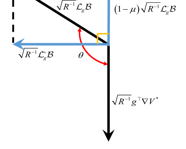
(a)

(b)

Figure 1: Gradient manipulation on $\sqrt{R^{-1}}\tilde{\mathcal{L}}_{g}\mathcal{B}$ when (a): $\mu=0$; and (b): $\mu=0.5$.

As shown in Fig.1, the gradient similarity $\rho$ increases monotonically with $\mu$ when $\theta\geq\frac{\pi}{2}$ , thus enhancing the system performance. This is rigorously analyzed in the following lemma.

Lemma 3.9.

Let $V^{*}$ be a continuously differentiable positive definite solution of (5). Then the following inequality holds

$$\int_{0}^{\infty}l(x(\tau),k^{*}(x(\tau))-K_{s}R^{-1}\mathcal{L}_{g}\mathcal{B}(x(\tau)))d\tau$$

$$\geq\int_{0}^{\infty}l(x(\tau),k^{*}(x(\tau))-K_{s}R^{-1}\tilde{\mathcal{L}}_{g}\mathcal{B}(x(\tau)))d\tau.$$ (18)

Proof 3.10.

Substituting $u(x)=k^{*}(x)-K_{s}R^{-1}\tilde{\mathcal{L}}_{g}\mathcal{B}(x)$ into (4), one has

$$H(x,\nabla V^{*},k^{*}(x)-K_{s}R^{-1}\tilde{\mathcal{L}}_{g}\mathcal{B}(x))$$

$$= \nabla_{x}V^{*T}(f(x)+g(x)(k^{*}(x)-K_{s}R^{-1}\tilde{\mathcal{L}}_{g}\mathcal{B}(x)))+x^{\top}Qx$$

$$+(k^{*}(x)-K_{s}R^{-1}\tilde{\mathcal{L}}_{g}\mathcal{B}(x)))^{\top}R(k^{*}(x)-K_{s}R^{-1}\tilde{\mathcal{L}}_{g}\mathcal{B}(x)))$$

$$= K_{s}^{2}(1-2\rho^{2}\mu+\rho^{2}\mu^{2})\lVert\sqrt{R^{-1}}\mathcal{L}_{g}\mathcal{B}\rVert^{2}.$$

Recalling (3.3) and the fact that $2\mu-\mu^{2}\geq 0$ (since $\mu\in[0,1)$), we have

$$H(x,\nabla V^{*},k^{*}(x)-K_{s}R^{-1}\tilde{\mathcal{L}}_{g}\mathcal{B}(x))$$

$$\leq H(x,\nabla V^{*},k^{*}(x)-K_{s}R^{-1}\mathcal{L}_{g}\mathcal{B}(x)).$$

Then inequality (3.9) holds according to Theorem 10.1-2 in [27].

On the other hand, additional control effort caused by $u^{s}$ can also be reduced by decreasing $K_{s}$. However, an unreasonably small $K_{s}$ can make the system unsafe. Then a natural question is how small $K_{s}$ should be. Before answering this question, we analyze how safety is affected by changes in $K_{s}$. Suppose $\psi_{m-1}(0)=0$ and then select a HO-RCBF satisfying $\lVert\nabla\mathcal{B}\rVert=\alpha_{B}(\mathcal{B})$, (e.g., $\mathcal{B}=\frac{1}{\psi_{m-1}}$ and $\lVert\nabla\mathcal{B}\rVert=\mathcal{B}^{2}$), where $\alpha_{B}$ is a class $\mathcal{K}$ function. Given $\omega\in\{x\in\mathbb{R}^{n}\;|\;\psi_{m-1}(x)=0\}$, there always exists a neighborhood $N(\omega)$ in which

$$\dot{\mathcal{B}}\leq\alpha_{B}(\mathcal{B})(\lVert\mathcal{L}_{f}\psi_{m-1}\rVert-K_{s}\bar{\sigma}(R)^{-1}\lVert\mathcal{L}_{g}\psi_{m-1}\rVert^{2}\alpha_{B}(\mathcal{B})).$$

Then we can obtain the upper bound of $\mathcal{B}$ as

$$\bar{\mathcal{B}}=\max\left(\mathcal{B}(0),\alpha_{B}^{-1}\left(\frac{\bar{\sigma}(R)\overline{\lVert\mathcal{L}_{f}\psi_{m-1}\rVert}_{N(\omega)}}{K_{s}\overline{\lVert\mathcal{L}_{g}\psi_{m-1}\rVert}_{N(\omega)}^{2}}\right)\right),$$

which implies that a small $K_{s}$ not only enhances performance but also allows a large value of $\mathcal{B}$. In practical situations, a controller is usually implemented in discrete-time using a zero-order hold (ZOH). As a result, the system under $u^{s}$ with a small $K_{s}$ can easily violate safety constraints during the sampling period if the control frequency at which the system measurements are fed back to recalculate the control input is not large enough. The influence of $K_{s}$ on safety guarantee is demonstrated in the following example.

Example 3.11.

Consider a mobile robot described by double integrator dynamics $\dot{p}=v$ and $\dot{v}=u$, where $p$ is the position, $v$ is the velocity, with the control $u=k(p,p_{d},v)+u^{s}(p,v)$, for the desired position trajectory, $p_{d}$, the control policy, $k=-v+100(p_{d}-p)$, steering $p$ to $p_{d}$ and $u^{s}$, the safeguarding policy. Suppose that the velocity constraint is described by $h(v)=v_{max}-v$, where $v_{max}$ is the maximum of $v$. We set the control frequency at $f_{c}=100$ Hz, and the sampling time at $0.01s$. We then define the RBCF as $B=\frac{1}{h(v)}$. The velocity and acceleration trajectories of the robot under different $K_{s}$ are given in Fig. 2.

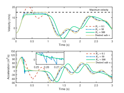
Figure 2: Velocity and acceleration trajectory of the mobile robot under $K_{s}=0.1$, $K_{s}=50$ and $K_{s}=500$. The maximum value of the velocity is $v_{max}=15m/s$.

When $K_{s}=0.1$, the safety constraint is violated due to the limitation of control frequency. Suppose $K_{s}$ is small enough such that

$$h(t_{k})=h_{\epsilon}\ \ \ \ \textnormal{and}\ \ \ \ \lVert u^{s}(t_{k})\rVert\leq k(t_{k})+\epsilon_{u}$$

for some $x\in N(\omega)$ at $t_{k}$, and $h_{\epsilon},\epsilon_{u}>0$. Then one has

$$\dot{h}(t)\leq-k(t_{k})+\lVert u^{s}(t_{k})\rVert\leq-\epsilon_{u}<0, \forall t\in[t_{k},t_{k+1})$$

which indicates $h(v)<0$ if $f_{c}<\frac{\epsilon_{u}}{h_{\epsilon}}$. Moreover, when $K_{s}=50$, the acceleration oscillates because the performance gradient and safety gradient switch rapidly when $v$ approaches $v_{max}$ (see [21] for more detailed discussion). Although a larger $K_{s}$ can address this issue, it also decreases the tracking performance by imposing a more conservative value of $v$ (see, e.g., the case when $K_{s}=500$).

Hence, a key question is how to design a suitable $K_{s}$ to guarantee the safety of the system while maintaining its performance. This motivates the following adaptive design approach. In practice, a large $K_{s,0}>0$ is initially needed to guarantee safety. Past the initial phase, the gain can then be updated adaptively to gain better system performance. To balance safety and performance, $K_{s}$ should be decreased to enhance performance when $\mathcal{B}$ is within a safety range and increased to guarantee safety when the control frequency is not large enough or the optimal control is large with a conflicting relationship $\rho<0$. Here, we define an auxiliary dynamic system for $K_{s}$ of the form

$$\dot{K}_{s}=F(x,K_{s})+G(x,K_{s})v$$ (19)

where $F:\mathbb{R}^{p+1}\rightarrow\mathbb{R}$ and $G:\mathbb{R}^{p+1}\rightarrow\mathbb{R}^{1\times q}$ are chosen such that $\lVert\mathcal{L}_{G}K_{s}\rVert\neq 0\;\forall x\in\mathbb{R}^{n},K_{s}\in\mathbb{R}$, and $v\in\mathbb{R}^{q}$ denote the control input for (19). As illustrated in Theorem 1 that the nonnegative property of $K_{s}$ can guarantee the safety of (1), we can regard the $K_{s}$ as a CBF, and define a constraint set $\mathcal{U}_{K}$ for $v$ as follows

$$\mathcal{U}_{K}=\{v\in\mathbb{R}^{q}\;|\;\mathcal{L}_{F}K_{s}+\mathcal{L}_{G}K_{s}v+\beta_{K}(K_{s})\geq 0\}$$

where $\beta_{K}$ is a class $\mathcal{K}$ function. For simplicity, let $F=0$ and $G=I$. Then we have $v\geq-\beta_{K}(K_{s})$. Hence, to guarantee $v\in\mathcal{U}_{K}$, we can directly set

$$v=-\beta_{K}(K_{s})+M(x,K_{s}),$$

where $M$ is a user-defined positive semi-definite function.

3.4 Adaptive high-order safeguarding policy

Combining the gradient manipulation approach and the adaptive mechanism of $K_{s}$, we propose an adaptive high-order safeguarding policy

$$u^{s} =-K_{s}R^{-1}\left((1-\mu)\mathcal{L}_{g}^{-}\mathcal{B}+\mathcal{L}_{g}^{+}\mathcal{B}\right)$$ (20)

$$\dot{K}_{s} =\operatorname{Proj}_{\mathcal{S}}\{-\beta_{K}(K_{s})+M(x,K_{s})\}$$ (21)

with $K_{s}(0)=K_{s,0}$ and

$$\beta_{K}(K_{s})=YK_{s}^{2}, M(x,K_{s})=\gamma e^{-h}l(x,k^{*}(x)),$$

where $\gamma>0$ is a weight used to increase $K_{s}$, ensuring safety, and $Y>0$ is a bounded value used to decrease $K_{s}$ if performance improvements are required. The operator $\operatorname{Proj}_{\mathcal{S}}\{\cdot\}$ guarantees that $K_{s}$ stays in a compact set $\mathcal{S}$, and is upper bounded by an arbitrary large $\bar{K}_{s}$, i.e., $\bar{K}_{s}=\mathop{\rm{sup}}_{K_{s}\in\mathcal{S}}\{K_{s}\}$. The function $M(x,K_{s})$ is designed to enable an increase of $K_{s}$ using a large $l(x,k^{*})$ and/or a small $h$ to balance the magnitude between a safeguarding policy and an optimal control policy. Using this adaptive safeguarding policy, we provide an adjustable control between safety and performance according to users’ requirements. By choosing a large $Y$ and a small $\gamma$, users can focus on achieving performance when the control frequency is large enough and there is no restriction on the magnitude of the input. On the other hand, choosing a small $Y$ and a large $\gamma$ allows users to emphasize safety over performance requirements.

Remark 3.12.

The HO-CBF provides a conservative safety guarantee since it serves only as a sufficient condition for ensuring the original safety requirements. To address this issue, approaches such as BarrierNet [29] and adaptive CBFs [33] have been proposed to enlarge the original safety set. In this paper, instead of addressing the conservativeness caused by HO-CBF itself, we pay more attention to conservativeness caused by the safeguarding approach in the following three ways. First, the safeguarding approach only needs to satisfy the CBF constraint

$$\mathcal{L}_{f}\mathcal{B}(\psi_{m-1})+\mathcal{L}_{g}\mathcal{B}(\psi_{m-1})u\leq\gamma_{3}\left(\psi_{m-1}\right)$$

for $x\in N(\omega)$ instead of all $x\in\{x\in\mathbb{R}^{n}\;|\;\psi_{m-1}(x)>0\}$. Second, the gradient manipulation approach is designed to enhance system performance. Third, the safeguarding gain is taken as an augmented CBF which provides the additional parameters $Y$ and $\gamma$, allowing more design freedom to balance safety and performance. BarrierNets or adaptive CBFs can be also combined with the adaptive safeguarding policy to further improve system performance.

In the following lemma, we show that the adaptive safeguarding policy (20) and $\eqref{e3.2.1b}$ can render $\bar{\mathscr{C}}$ forward invariant.

Lemma 3.13.

Given any $x_{0}\in\operatorname{Int}(\mathscr{C})$, define the functions (8) and the corresponding sets (9) satisfying $x_{0}\in\bar{\mathscr{C}}$. Under Assumptions 1-2, the adaptive safeguarding controller $\eqref{e3.2.1a}$ and $\eqref{e3.2.1b}$ can render the safety set of both the nominal system (2) and system (1) forward invariant, i.e., $x(t)\in\bar{\mathscr{C}}$ for all $t\geq 0$ and $x_{0}\in\bar{\mathscr{C}}$.

Proof 3.14.

By Assumption 2, there exists a neighborhood $N_{l}$ of the origin such that $N_{l}\cap\mathscr{C}^{S}=\emptyset$, which implies $h(x)>0\;\forall x\in N_{l}$. Therefore, one can always find some extended class $\mathcal{K}$ functions $\alpha_{1},\alpha_{2},\dots,\alpha_{m-1}$ in (8) such that

$$\psi_{1}(x),\ \psi_{2}(x),\ \dots,\ \psi_{m-1}(x)>0, \forall x\in N_{l}.$$

Hence, for the derived set $\mathscr{C}_{m}^{S}$ of $\mathscr{C}_{m}$, one has $N_{l}\cap\mathscr{C}_{m}^{S}=\emptyset$. Since $0\notin\mathscr{C}_{m}^{S}$, we consider a set $B_{l}=\{x\in\mathbb{R}^{n}\;|\;\lVert x\rVert<l\}$, where $l>0$ is an arbitrary positive constant such that $B_{l}\subset N_{l}$. For any $K_{s}(0)>0$, $h=0$ and $\forall x\in\mathbb{R}^{n}\backslash B_{l}$, one has

$$\dot{K}_{s}(t)\geq\gamma\underline{\sigma}(Q)r^{2}-Y\lVert K_{s}(t)\rVert^{2}.$$

Hence we have $K_{s}(t)\geq\frac{r^{2}}{Y}\underline{\sigma}(Q)\gamma$ for all $x\in\mathbb{R}^{n}\backslash B_{l}$ if $h$ get close to zero. The time derivative of $\mathcal{B}(x)$ along the state trajectories is

$$\dot{\mathcal{B}}(x)\leq \ \lVert\nabla\mathcal{B}(x)\rVert\left(\lVert\mathcal{L}_{f}\psi_{m-1}\rVert+\lVert\mathcal{L}_{g}\psi_{m-1}\rVert\lVert u^{f}\rVert\right)$$

$$-(1-\rho^{2}\mu)K_{s}\nabla\mathcal{B}(x)^{\top}\mathcal{L}_{g}\psi_{m-1}R^{-1}\mathcal{L}_{g}\psi_{m-1}^{\top}\nabla\mathcal{B}(x).$$

Since $\rho^{2}\leq 1$ and $\mu<1$, we have $1-\rho^{2}\mu>0$. From $\mathscr{C}_{m}^{S}\subset\mathbb{R}^{n}\backslash B_{l}$ and $(1-\rho^{2}\mu)K_{s}>0$, the safeguarding controller can guarantee ${\color[rgb]{0,0,0}\mathcal{B}}<\infty$ for both (2) and (1) according to Assumption 1 and Theorem 1. For any $x\in B_{l}$, the safety can always be guaranteed. Hence, for the nominal system (2) and system (1), the adaptive safeguarding controller (20) with its adaptation law (21) can render the set $\bar{\mathscr{C}}$ forward invariant.

The following corollary shows how the adaptive safeguarding control policy guarantees the safety of system (1) and its nominal system (2) under a stabilizing control policy.

Corollary 3.15.

Suppose Assumptions 1-2 hold. Let $k(x,t)$ be a nominal stabilizing control policy that is locally Lipschitz in $x$ on $B_{r}$ and piecewise continuous in $t$, and satisfies $k(0,t)=0$. Given any $x_{0}\in\operatorname{Int}(\mathscr{C})$, define a series of functions (8) and corresponding sets (9) such that $x_{0}\in\bar{\mathscr{C}}$. Then for the nominal system (2) and system (1), the state trajectories under $k(x,t)$ and the adaptive safeguarding policy (20), (21) always stay in $\bar{\mathscr{C}}$.

Proof 3.16.

Invoking Lemma 3.13, we can proceed following the proof of Corollary 3.6.

From Corollary 3.15, the function $\mathcal{B}(x)$ corresponding to system (2) is bounded under the optimal control policy (6) and the adaptive safeguarding policy (20), (21). Since $\mathcal{B}(x)$ is continuously differentiable, it follows that $\nabla_{x}\mathcal{B}(x)$ is bounded. Suppose that the state trajectories of (2) under the adaptive safeguarding policy (20), (21) and the optimal control policy (6) always stay in the admissible safety risk set $\mathscr{B}:=\{x\in\mathbb{R}^{n}\;|\;\lVert\nabla_{x}\mathcal{B}(x)\rVert^{2}\leq W\}$, where $W$ is a positive constant. Now we shall provide a sufficient condition to guarantee the stability of the closed-loop system.

Theorem 2.

Let $V^{*}$ be a continuously differentiable positive definite solution of (5) and $\mathscr{B}$ be the admissible safety risk set. Let $\rho$ be defined by (16). Suppose $x_{0}\in\operatorname{Int}(\mathscr{C})$, Assumption 2 holds and the optimal control policy $k^{*}(x)$ is locally Lipschitz in $x$. Applying the unconstrained optimal control policy (6), the adaptive safeguarding policy (20) and (21) to the nominal systems (2), the origin is asymptotically stable equilibrium of the closed-loop system under either of the following conditions

• $0<\gamma<1$, and $\rho(x)\geq 0,~\forall x\in\mathscr{B}$;

• $0<\gamma<1$, $0\leq\mu<1$, $Y>\frac{(1-\mu)^{2}}{1-\gamma}\frac{W\bar{g}^{2}}{\underline{\sigma}(R)}$, and $\rho(x)<0$ for some $x\in\mathscr{B}$.

Proof 3.17.

Consider the following Lyapunov function candidate $L_{x}(x,K_{s})=V^{*}(x)+K_{s}$. Under the optimal control policy (6), the safeguarding policy (20) and its adaptation law (21), the time derivative of $V^{*}(x)$ along (2) becomes

$$\dot{V}^{*}(x)=\nabla V^{*}(x)^{\top}\left(f(x)+g(x)(u^{s}(x)+k^{*}(x))\right).$$ (22)

Define $G_{R}(x)=g(x)R^{-1}g(x)^{\top}$. Combining (5), (6), (13) and (22) yields

$$\dot{V}^{*}(x)= -x^{\top}Qx-\frac{1}{4}\nabla V^{*}(x)^{\top}G_{R}(x)\nabla V^{*}(x)$$

$$-K_{s}(1-\mu)\nabla V^{*}(x)^{\top}G_{R}(x)\nabla_{x}\mathcal{B}(x).$$

According to Theorem 3.10.1 in [34], the time derivative of $L_{x}$ along (2) and (21) is

$$\dot{L}_{x}\leq -(1-\gamma)\left(x^{\top}Qx+\frac{1}{4}\lVert\sqrt{R^{-1}}g^{\top}\nabla V^{*}\rVert^{2}\right)$$

$$-YK_{s}^{2}-K_{s}(1-\mu)\nabla V^{*}(x)^{\top}G_{R}(x)\nabla_{x}\mathcal{B}(x).$$

• Under condition C1, involving (16) and $K_{s}\geq 0$, the time derivative of $V^{*}$ is

  $$\dot{V}^{*}\leq-x^{\top}Qx-\frac{1}{4}\lVert\sqrt{R^{-1}}g^{\top}\nabla V^{*}\rVert^{2},$$

  and $\dot{L}_{x}$ is given as

  $$\dot{L}_{x}\leq-(1-\gamma)\left(x^{\top}Qx+\frac{1}{4}\lVert\sqrt{R^{-1}}g^{\top}\nabla V^{*}\rVert^{2}\right)-YK_{s}^{2}.$$

  Hence, the Lyapunov stability condition is always satisfied when $\rho\geq 0$.

• Under condition C2, if a constant $K_{s}$ is adopted, the stability of the closed-loop system might be destroyed due to the conflict between $u^{s}$ and $k^{*}$, i.e., $\rho<0$. However, the stability condition of $L_{x}$ can still be guaranteed by the adaptive law (20), (21). The time derivative of $L_{x}$ can be obtained as

  $$\dot{L}_{x}\leq -(1-\gamma)\left(x^{\top}Qx+\frac{1}{4}\lVert\sqrt{R^{-1}}g^{\top}\nabla V^{*}\rVert^{2}\right)-YK_{s}^{2}$$

  $$-(1-\mu)\rho\lVert\sqrt{R^{-1}}g^{\top}\nabla V^{*}\rVert\lVert\sqrt{R^{-1}}g^{\top}\nabla_{x}\mathcal{B}(x)\rVert K_{s}.$$

  Completing the squares and considering the fact that $\lVert\rho\rVert\leq 1$, one further has

  $$\dot{L}_{x}\leq -(1-\gamma)\left(x^{\top}Qx+\frac{\lVert\sqrt{R^{-1}}g^{\top}\nabla V^{*}\rVert^{2}}{4Y}\big{(}Y\right.$$

  $$\left.-\frac{(1-\mu)^{2}}{1-\gamma}\lVert\sqrt{R^{-1}}g^{\top}\nabla_{x}\mathcal{B}(x)\rVert^{2}\big{)}\right).$$

  Since Assumption 2 holds, one has

  $$\lVert G_{R}(x)\rVert\leq\bar{g}^{2}\underline{\sigma}(R)^{-1}.$$

  Given $(1-\gamma)Y>(1-\mu)^{2}\frac{W\bar{g}^{2}}{\underline{\sigma}(R)}$ and $\gamma<1$, we have

  $$\dot{L}_{x}\leq-(1-\gamma)x^{\top}Qx,$$

  for any $x\in\mathscr{B}$.

Therefore, under both conditions C1 and C2, one has $L_{x}(t)\leq L_{x}(0),\forall t\geq 0$. According to LaSalle’s invariance principle, one can conclude that $\mathop{lim}_{t\rightarrow\infty}x(t)=0$. Hence, asymptotic stability of the system (2) is achieved under the adaptive safeguarding policy (20) and (21), and the optimal control policy (6).

4 Online implementation of adaptive safe RL

This section develops an adaptive safe exploration framework for learning $V^{*}(x)$ and $k^{*}(x)$ while guaranteeing safety and robustness based on an adaptive high-order safeguarding policy, a nonlinear disturbance/actuator fault observer and actor-critic neural networks (NNs).

4.1 Disturbance/fault observer design

To compensate for unknown disturbance/fault $u^{f}$, the following nonlinear disturbance/fault observer [22] is adopted

$$\hat{u}^{f}(t) =z(t)+\omega(x),$$

$$\dot{z}(t) =-L(x)\left(f(x)+g(x)\left(u(t)+z(t)+\omega(x)\right)\right),$$ (23)

where $\hat{u}^{f}$ is the estimation of $u^{f}$, $z$ is an auxiliary vector, $L^{\top}(x)=\partial\omega(x)/\partial x$ and $\omega(x)$ is a user-defined function.

Let the estimation error be $\tilde{u}^{f}=u^{f}-\hat{u}^{f}$. Its dynamics are given by

$$\dot{\tilde{u}}^{f}=-L(x)g(x)\tilde{u}^{f}+\dot{u}^{f}.$$

An appropriate $\omega(x)$ is chosen such that $L(x)g(x)$ is positive definite. Then one can find a positive definite function $L_{u}(\tilde{u}^{f})$ such that

$$\dot{L}_{u}(\tilde{u}^{f})\leq-K_{f}\lVert\tilde{u}^{f}\rVert^{2}+K_{d}\lVert\tilde{u}^{f}\rVert$$ (24)

for all $\tilde{u}_{f}\in\mathbb{R}^{p}$, where $K_{f},K_{d}>0$, and $K_{d}$ depends on the upper bound of $\dot{u}^{f}$, i.e., $\eta_{2}$ defined in Assumption 1. According to (24), one has $\lVert\tilde{u}_{f}\rVert\leq\bar{\tilde{u}}^{f}$, where $\bar{\tilde{u}}^{f}=\max\{{K_{d}}/{K_{f}},\lVert\tilde{u}^{f}_{0}\rVert\}$ and $\tilde{u}^{f}_{0}=u^{f}(0)-\hat{u}^{f}(0)$.

Remark 4.1.

Using observer (4.1), Assumption 1 can be relaxed to allow $u^{f}$ to be unbounded, as long as its derivative is bounded, i.e.,

$$u^{f}(t)\in\{u^{f}(t)\in\mathbb{R}^{p}\;|\;\lVert\dot{u}^{f}\rVert_{\infty}\leq\eta\},$$ (25)

where $\eta$ is an unknown positive constant. Regarding $\tilde{u}^{f}$ as a new disturbance/fault, one has

$$\dot{\mathcal{B}}(x)\leq\lVert\nabla\mathcal{B}(x)\rVert^{2}\left(\frac{L_{\psi}}{\lVert\nabla\mathcal{B}(x)\rVert}-\frac{K_{s}}{\bar{\sigma}(R)}\lVert\mathcal{L}_{g}\psi_{m-1}\rVert^{2}\right),$$

where $L_{\psi}=\lVert\mathcal{L}_{f}\psi_{m-1}\rVert+\lVert\mathcal{L}_{g}\psi_{m-1}\rVert\bar{\tilde{u}}^{f}$. From Theorem 1, the safeguarding policy (13) can still guarantee safety in the presence of any unknown unbounded $u^{f}$ with the aid of (4.1). Recalling Lemma 3.13, safety under the adaptive safeguarding policy (20) and (21) subject to an unbounded disturbance/fault, $u^{f}$, can also be guaranteed.

4.2 Actor-critic neural networks

Over a compact set $\mathcal{X}\in\mathbb{R}^{n}$, the optimal value function $V^{*}(x)$ can be approximated as

$$V^{*}(x)=W^{\top}\phi(x)+\varepsilon(x)$$

where $W\in\mathbb{R}^{s}$ is the ideal approximation weight, $\phi:\mathbb{R}^{n}\rightarrow\mathbb{R}^{s}$ is the activation function with $\phi(0)=0$ and $\nabla\phi(0)=0$, and $\varepsilon:\mathbb{R}^{n}\rightarrow\mathbb{R}$ is the approximation error. By the universal function approximation property [35], the approximation error $\varepsilon(x)$ can made be arbitrarily small and bounded by a given positive constant $\bar{\varepsilon}$.

The derivative of $V^{*}(x)$ along the state trajectory is given as follows

$$\nabla V^{*}(x)=\nabla\phi(x)^{\top}W+\nabla\varepsilon(x),$$

where $\nabla\varepsilon(x)$ is bounded by some positive constant $\bar{\varepsilon}_{\nabla}$ over the compact set $\mathcal{X}$. Since the ideal weight $W$ is unknown, a critic NN (26) and an actor NN (27) are utilized to approximate the optimal value function and the optimal stabilizing control policy

$$\hat{V}(x) =\hat{W}_{c}^{\top}\phi(x),$$ (26)

$$K(x,t) =-\frac{1}{2}R^{-1}g(x)^{\top}\nabla\phi(x)^{\top}\hat{W}_{a}(t),$$ (27)

where $\hat{W}_{c}$ is the critic NN weight and $\hat{W}_{a}$ is the actor NN weight.

4.3 Safe RL via simulation of experience

This section develops an adaptive safe exploration framework for learning the optimal value function and optimal control policy based on simulation of experience. The behavior policy is defined as

$$u=K(x,t)+u^{s}(x,K_{s})-\hat{u}^{f},$$ (28)

where the first term is the target policy, the second term is the safeguarding policy, and the last term is the estimated disturbance/fault. The Bellman error is defined as

$$\delta=\hat{W}_{c}^{\top}\varphi+l(x,u),$$ (29)

where $\nabla\phi=\partial\phi/\partial x$ and $\varphi=\nabla\phi(x)(f(x)+g(x)u)$. Given that online learning is actually off-policy since the behavior policy (28) is different from $K$, the collected data may result in an approximation error in the optimal control policy (6). Hence, the nominal system is utilized to generate simulation data to correct the approximation error and relax the PE condition as well. Denote $\{x_{i}(t)\}_{i=1}^{N}$ as a collection of $N$ state points sampled from $\mathcal{X}$ at $t\geq 0$ and $u_{i}=K(x_{i},t)$ as the exploratory policy. The Bellman error at each sampled state is obtained as

$$\delta_{i}=\hat{W}_{c}^{\top}\varphi_{i}+l(x_{i},u_{i}),$$ (30)

where $\varphi_{i}=\nabla\phi(x_{i})(f(x_{i})+g(x_{i})u_{i})$. The tuning law for the critic NN weights is

$$\dot{\hat{W}}_{c} =-\Gamma\Big{(}k_{c1}\frac{\varphi}{\rho^{2}}\delta+\frac{k_{c2}}{N}\sum_{i=1}^{N}\frac{\varphi_{i}}{\rho_{i}^{2}(t)}\delta_{i}\Big{)}$$ (31)

$$\dot{\Gamma} =\beta\Gamma-\Gamma\Big{(}k_{c1}\Lambda+\frac{k_{c2}}{N}\sum_{i=1}^{N}\Lambda_{i}\Big{)}\Gamma$$ (32)

where $\rho(t)=1+\varphi(t)^{\top}\varphi(t)$, $\rho_{i}(t)=1+\varphi_{i}(t)^{\top}\varphi_{i}(t)$,

$$\Gamma(0)>0,\ \Lambda(t)=\frac{\varphi(t){\varphi(t)}^{\top}}{\rho^{2}(t)}\ \ \textnormal{and}\ \ \Lambda_{i}(t)=\frac{\varphi_{i}(t){\varphi_{i}(t)}^{\top}}{\rho_{i}^{2}(t)},$$

are normalizing signals, $k_{c1},k_{c2}>0$ are learning gains, and $\beta>0$ is a forgetting factor. Let $G_{\phi}=\nabla\phi(x)G_{R}(x)\nabla\phi(x)^{\top}$ and $G_{\phi,i}=\nabla\phi(x_{i})G_{R}(x_{i})\nabla\phi(x_{i})^{\top}$. The tuning law of the actor NN weights is

$$\dot{\hat{W}}_{a}= \operatorname{Proj}_{\mathcal{W}}\biggl{\{}-k_{a1}\left(\hat{W}_{a}-\hat{W}_{c}\right)+\frac{k_{c1}}{4\rho^{2}}G_{\phi}\hat{W}_{a}\varphi^{\top}\hat{W}_{c}$$

$$-k_{a2}\hat{W}_{a}+\sum_{i=1}^{N}\frac{k_{c2}}{4N\rho_{i}^{2}}G_{\phi,i}\hat{W}_{a}\varphi_{i}^{\top}\hat{W}_{c}\biggl{\}},$$ (33)

where $k_{a1},k_{a2}>0$ are learning gains, and $\operatorname{Proj}_{\mathcal{W}}\{\cdot\}$ is a projection operator for keeping the actor NN estimation within a compact set $\mathcal{W}\in\mathbb{R}^{s}$.

To provide a PE-like condition that can be easily checked during the learning process, and facilitate the stability analysis, we make the following assumption.

Assumption 3

Given the NNs (26) and (27), the following conditions hold:

1. The optimal weights $W$ are norm-bounded by an unknown positive constant $\bar{W}$.

2. The activation function $\phi(x)$ and its derivative $\nabla\phi(x)$ are norm-bounded by positive constants $\bar{\phi}$ and $\bar{\phi}_{\nabla}$ on $\mathcal{X}$, respectively.

3. The sample number $N$ is large enough to satisfy the following PE-like condition

   $$\inf_{t\geq 0}\left\{\underline{\sigma}\left(\frac{1}{N}\sum_{i=1}^{N}\Lambda_{i}(t)\right)\right\}\geq\lambda_{c},$$

   where $\lambda_{c}$ is a positive constant.

Remark 4.2.

Assumption 3 is standard in solving optimal control problem using RL [36]. The first assumption is made to exclude the non-existence solution. The second assumption can be satisfied by taking sigmoid, Gaussian and other standard NN activation functions [37]. The last condition can be satisfied by choosing a large number of sampled data [38].

4.4 Safety and stability analysis

In this section, we analyze the safety and stability of the closed-loop system under the control policy (28).

Lemma 4.3.

Consider the system (1). Suppose Assumptions 2-3, condition (25) and inequality (24) hold. The control policy (28) along with the actor weight update law (4.3), the disturbance observer (4.1), and the safeguarding gain adaptive law (21) can render the safety set $\bar{\mathscr{C}}$ forward invariant for the closed-loop system

$$\dot{x}=f(x)+g(x)(K(x,t)+u^{s}(x,K_{s})).$$

Proof 4.4.

Suppose condition (25) and the inequality (24) hold. One has that $\tilde{u}^{f}$ is norm-bounded. By Assumptions 2 and 3, one has

$$\lVert g(x)^{\top}\nabla\phi(x)^{\top}\rVert\leq\bar{g}\bar{\phi}_{\nabla}.$$

Then it follows that $K(x,t)$ is norm-bounded by $\frac{1}{2\underline{\sigma}(R)}\bar{g}\bar{\phi}_{\nabla}\bar{W}_{a}$ since $\hat{W}_{a}$ is norm-bounded in a compact set using the projection operator. Recalling that $\tilde{u}^{f}(t)$ and $K(x,t)$ are norm-bounded, Lemma 1 implies that the safety set $\bar{\mathscr{C}}$ is forward invariant.

Let $V^{*}$ and $k^{*}$ be approximated on some compact set $\mathcal{X}$. Define the weight estimation errors as

$$\tilde{W}_{c}=W-\hat{W}_{c}\ \ \textnormal{and}\ \ \tilde{W}_{a}=W-\hat{W}_{a},$$

and a composite state $z=\textnormal{col}\bm{(}x,\tilde{W}_{c},\tilde{W}_{c},\tilde{u}_{f},K_{s}\bm{)}$. To guarantee that the value function approximation error $\varepsilon(x)$ and its derivative $\nabla\varepsilon(x)$ are norm-bounded during the learning process, one can construct a compact set $\mathcal{Z}\subset\mathcal{X}\times\mathbb{R}^{2s+p+1}$ that contains the composite state trajectory. Define $\bar{\varepsilon}=\overline{\lVert\varepsilon(x)\rVert}_{\mathcal{X}}$ and $\bar{\varepsilon}_{\nabla}=\overline{\lVert\nabla\varepsilon(x)\rVert}_{\mathcal{X}}$. The following theorem illustrates that the robust and adaptive safe exploration method ensures the composite state is uniformly ultimately bounded (UUB).

Theorem 3.

Consider the nonlinear system (1) and the safety set $\mathscr{C}$ with $0\in\mathscr{C}$ and $x(0)\in\operatorname{Int}(\mathscr{C})$. Define a series of functions (8) and sets (9) corresponding to the safety set $\mathscr{C}$. Let the safeguarding controller and its adaptive law be given by (20) and (21), the actuator disturbance/fault observer be constructed as (4.1), the optimal value function and corresponding control policy be approximated by NNs over a compact set $\mathcal{X}$ with the critic NN updated by (31) and (32), and the actor NN updated by (4.3), respectively. Suppose that Assumptions 2-3, condition (25) and inequality (24) hold. Then the control policy (28) guarantees that the composite state $z(t)$ is UUB.

Proof 4.5.

The closed-loop system is

$$\dot{x}=f(x)+g(x)(K(x,t)+u^{s}(x,K_{s})+\tilde{u}^{f}).$$ (34)

Consider the following Lyapunov function candidate

$$\hskip-7.22743ptP(z,t)=L_{x}(x,K_{s})+L_{c}(\tilde{W}_{c},t)+L_{a}(\tilde{W}_{a})+L_{u}(\tilde{u}^{f})$$ (35)

where $L_{c}(\tilde{W}_{c},t)=\frac{1}{2}\tilde{W}_{c}^{\top}\Gamma^{-1}(t)\tilde{W}_{c}$, $L_{a}(\tilde{W}_{a})=\frac{1}{2}\tilde{W}_{a}^{\top}\tilde{W}_{a}$ and $L_{u}(\tilde{u}^{f})$ is a positive definite function satisfying (24).

Under Assumption 3, there exist positive constants $\bar{\Gamma}$ and $\underline{\Gamma}$ such that $\bar{\Gamma}I\leq\Gamma(t)\leq\underline{\Gamma}I$, $\forall t\geq 0$ ([39], Lemma 1). Therefore, $P(z,t)$ is positive definite and hence

$$\eta_{1}(\lVert z\rVert)\leq P(z,t)\leq\eta_{2}(\lVert z\rVert)$$

for some class $\mathcal{K}$ functions $\eta_{1}$ and $\eta_{2}$ [28].

The time derivative of $V^{*}$ along the system (34) is

$$\dot{V}^{*}=\nabla{V^{*}}^{\top}\left(f(x)+g(x)(K(x,t)+u^{s}(x,K_{s})+\tilde{u}^{f})\right)$$

Noting that $H(x,\nabla V^{*},k^{*})=0$, one has

$$\dot{V}^{*}=-x^{\top}Qx-{k^{*}}^{\top}Rk^{*}+\nabla{V^{*}}^{\top}g(x)(u^{s}+\tilde{u}^{f}-\tilde{k})$$ (36)

where

$$\tilde{k}=k^{*}-K(x,t)=-\frac{1}{2}R^{-1}g(x)^{\top}(\nabla\phi^{\top}\tilde{W}_{a}+\nabla\varepsilon).$$

Taking (20), (21) and (36) into consideration, the time derivative of $L_{x}$ is

$$\dot{L}_{x}\leq -(1-\gamma)x^{\top}Qx+\frac{1}{2}W^{\top}G_{\phi}\tilde{W}_{a}-YK_{s}^{2}+\frac{\gamma}{4}\hat{W}_{a}^{\top}G_{\phi}\hat{W}_{a}$$

$$+\frac{1}{2}\nabla\varepsilon^{\top}G_{R}\nabla\phi^{\top}\tilde{W}_{a}+(W^{\top}\nabla\phi+\nabla\varepsilon^{\top})g(x)\tilde{u}_{f}$$

$$-(W^{\top}\nabla\phi+\nabla\varepsilon^{\top})G_{R}\nabla_{x}\mathcal{B}K_{s}+\bar{\varepsilon}_{1}$$

$$\leq -(1-\gamma)x^{\top}Qx-YK_{s}^{2}+\frac{\gamma}{4}\bar{G}_{\phi}\lVert W\rVert^{2}+\frac{\gamma}{4}\bar{G}_{\phi}\lVert\tilde{W}_{a}\rVert^{2}$$

$$+\frac{l_{1}}{2}\lVert\tilde{W}_{a}\rVert+l_{2}\bar{g}\lVert\tilde{u}_{f}\rVert+l_{2}\bar{K}_{s}\bar{G}_{R}\lVert\nabla_{x}\mathcal{B}\rVert_{\infty}+\bar{\varepsilon}_{1}$$ (37)

where $\bar{G}_{R}=\bar{\sigma}(R)\bar{g}^{2}$, $\bar{G}_{\phi}=\bar{G}_{R}\bar{\phi}_{\nabla}^{2}$,

$$\bar{\varepsilon}_{1} =\frac{1}{2}\overline{\lVert W^{\top}\nabla\phi G_{R}\nabla\varepsilon+G_{\varepsilon}\rVert}_{\mathcal{X}},\quad G_{\varepsilon}=\nabla\varepsilon^{\top}G_{R}\nabla\varepsilon,$$

$$l_{1} =(1-\gamma)\bar{W}\bar{G}_{\phi}+\bar{\varepsilon}_{\nabla}\bar{G}_{R}\bar{\phi}_{\nabla},\quad l_{2}=\bar{W}\bar{\phi}_{\nabla}+\bar{\varepsilon}_{\nabla}.$$

The time derivative of $L_{c}$ is

$$\dot{L}_{c}=\tilde{W}_{c}^{\top}\Gamma^{-1}\dot{\tilde{W}}_{c}-\frac{1}{2}\tilde{W}_{c}^{\top}\Gamma^{-1}\dot{\Gamma}\Gamma^{-1}\tilde{W}_{c}$$ (38)

where

$$\dot{\tilde{W}}_{c}=\Gamma\left(k_{c1}\frac{\varphi}{\rho^{2}}\delta+\frac{k_{c2}}{N}\sum_{i=1}^{N}\frac{\varphi_{i}}{\rho_{i}^{2}}\delta_{i}\right).$$ (39)

Based on the fact that

$$K^{\top}RK=\frac{1}{4}W^{\top}G_{\phi}W+\frac{1}{4}\tilde{W}_{a}^{\top}G_{\phi}\tilde{W}_{a}-\frac{1}{2}W^{\top}G_{\phi}\tilde{W}_{a}$$

and $H(x,\nabla V^{*},k^{*})=0$, one has

$$W^{\top}\nabla\phi f(x)+x^{\top}Qx-\frac{1}{4}W^{\top}G_{\phi}W$$

$$=\frac{1}{4}\varepsilon^{\top}G_{R}\varepsilon+\frac{1}{2}\nabla\varepsilon^{\top}G_{R}\nabla\phi^{\top}W-\nabla\varepsilon^{\top}f(x)$$

and then the Bellman error (29) can be rewritten as

$$\delta= -\varphi^{\top}\tilde{W}_{c}+x^{\top}Qx+u^{\top}Ru+\varphi^{\top}W$$

$$= -\varphi^{\top}\tilde{W}_{c}+\frac{1}{4}\tilde{W}_{a}^{\top}G_{\phi}\tilde{W}_{a}+\varepsilon_{H}+\xi,$$ (40)

where

$$\varepsilon_{H}=\frac{1}{4}\varepsilon^{\top}G_{R}\varepsilon+\frac{1}{2}\nabla\varepsilon^{\top}G_{R}\nabla\phi^{\top}W-\nabla\varepsilon^{\top}f(x)$$

and

$$\xi=-\tilde{W}_{a}^{\top}\nabla\phi G_{R}\nabla_{x}\mathcal{B}K_{s}-\tilde{W}_{a}^{\top}\nabla\phi g(x)u^{f}+\tilde{W}_{a}^{\top}\nabla\phi g(x)\tilde{u}^{f}$$

$$+\nabla_{x}\mathcal{B}^{\top}G_{R}\nabla_{x}\mathcal{B}K_{s}^{2}+2\nabla_{x}\mathcal{B}^{\top}g(x)u^{f}\hat{K_{s}}-2K_{s}\nabla_{x}\mathcal{B}^{\top}g(x)\tilde{u}^{f}$$

$$+u^{fT}Ru^{f}+\tilde{u}^{fT}R\tilde{u}^{f}-2u^{fT}R\tilde{u}^{f}.$$

Similarly, the Bellman error (30) estimated at $x_{i}$, sampled from the compact set $\mathcal{X}$, can be obtained as

$$\delta_{i} =\hat{W}_{c}^{\top}\nabla\phi_{i}(f_{i}(x)+g_{i}(x)K_{i})+x_{i}^{\top}Qx_{i}+K_{i}^{\top}RK_{i},$$

$$=-\varphi_{i}^{\top}\tilde{W}_{c}+\frac{1}{4}\tilde{W}_{a}^{\top}G_{\phi,i}\tilde{W}_{a}+\varepsilon_{H,i},$$ (41)

where $\varepsilon_{H,i}=\varepsilon_{H}(x_{i})$ and $K_{i}=K(x_{i})$.

Combining (39), (4.5) and (4.5), (38) can be put as

$$\dot{L}_{c}= -\frac{1}{2}\tilde{W}_{c}^{\top}\left(\beta\Gamma^{-1}+k_{c1}\Lambda+\frac{k_{c2}}{N}\sum_{i=1}^{N}\Lambda_{i}\right)\tilde{W}_{c}$$

$$+\tilde{W}_{c}^{\top}\left(k_{c1}\frac{\varphi}{\rho^{2}}\varepsilon_{H}+\frac{k_{c2}}{N}\sum_{i=1}^{N}\frac{\varphi_{i}}{\rho_{i}^{2}}\varepsilon_{H,i}\right)$$

$$+\tilde{W}_{c}^{\top}k_{c1}\frac{\varphi}{\rho^{2}}\xi+\frac{1}{4}\tilde{W}_{c}^{\top}\varrho,$$ (42)

where

$$\varrho=k_{c1}\frac{\varphi}{\rho^{2}}\tilde{W}_{a}^{\top}G_{\phi}\tilde{W}_{a}+\frac{k_{c2}}{N}\sum_{i=1}^{N}\frac{\varphi_{i}}{\rho_{i}^{2}}\tilde{W}_{a}^{\top}G_{\phi,i}\tilde{W}_{a}.$$

Since $f(x)$ is locally Lipschitz, its Lipschitz constant is bounded in the compact set $\mathcal{X}$. Define $\bar{\varepsilon}_{H}=\overline{\lVert\varepsilon_{H}\rVert}_{\mathcal{X}}$. Using the fact that the inequality

$$\left\lVert\frac{w}{(1+w^{\top}w)^{2}}\right\rVert\leq\frac{3\sqrt{3}}{16}$$

always holds for any vector $w\in\mathbb{R}^{q}$, we further have

$$\dot{L}_{c}\leq -k_{c2}\bar{\lambda}_{c}\lVert\tilde{W}_{c}\rVert^{2}+\frac{3\sqrt{3}}{16}\bar{k}_{c}\bar{\varepsilon}_{H}\lVert\tilde{W}_{c}\rVert$$

$$+\tilde{W}_{c}^{\top}k_{c1}\frac{\varphi}{\rho^{2}}\xi+\frac{1}{4}\tilde{W}_{c}^{\top}\varrho,$$ (43)

where $\bar{\lambda}_{c}=\frac{\beta}{2k_{c2}\bar{\Gamma}}+\frac{\lambda_{c}}{2}$ and $\bar{k}_{c}=k_{c1}+k_{c2}$.

Since the projector in (4.3) guarantees $\lVert\hat{W}_{a}\rVert\leq\bar{W}_{a}$ for some $\bar{W}_{a}>0$ in a compact set $\mathcal{W}$, one has

$$\lVert\tilde{W}_{a}\rVert\leq\lVert\hat{W}_{a}\rVert+\lVert W\rVert,$$

i.e., $\tilde{W}_{a}$ is norm-bounded by $\bar{W}_{a}+\bar{W}$. Due to the fact that $\tilde{W}_{a}$ and $\tilde{u}_{f}$ are norm-bounded, the inequality $\dot{L}_{x}$ (4.5) implies that $x$ and $\hat{K_{s}}$ are norm-bounded. Hence, one can obtain the following inequalities

$$\tilde{W}_{c}^{\top}k_{c1}\frac{\varphi}{\rho^{2}}\xi\leq k_{c1}\frac{3\sqrt{3}}{16}\lVert\tilde{W}_{c}\rVert\lVert\xi\rVert$$ (44)

and

$$\lVert\xi\rVert\leq \left(\bar{K}_{s}\bar{G}_{R}\lVert\nabla_{x}\mathcal{B}\rVert_{\infty}+(\eta_{1}+\bar{\tilde{u}}^{f})\bar{g}\right)\bar{\phi}_{\nabla}\lVert\tilde{W}_{a}\rVert$$

$$+2(\eta_{1}\bar{\sigma}(R)+\bar{g}\bar{K}_{s}\lVert\nabla_{x}\mathcal{B}\rVert_{\infty})\lVert\tilde{u}^{f}\rVert$$

$$+2\eta_{1}\bar{g}\lVert\nabla_{x}\mathcal{B}\rVert_{\infty}\lVert K_{s}\rVert+\bar{\sigma}(R)\left(\eta_{1}^{2}+(\bar{\tilde{u}}^{f})^{2}\right)$$

$$+\bar{K}_{s}^{2}\bar{G}_{R}\lVert\nabla_{x}\mathcal{B}\rVert_{\infty}^{2}.$$ (45)

Similarly, taking the time derivative of $L_{a}$ along (4.3) yields

$$\dot{L}_{a}\leq -\bar{k}_{a}\tilde{W}_{a}^{\top}\tilde{W}_{a}+k_{a1}\tilde{W}_{a}^{\top}\tilde{W}_{c}+k_{a2}\tilde{W}_{a}^{\top}W$$

$$-k_{c1}\tilde{W}_{a}^{\top}\frac{G_{\phi}}{4\rho^{2}}\hat{W}_{a}\varphi^{\top}\hat{W}_{c}-\frac{k_{c2}}{N}\sum_{i=1}^{N}\tilde{W}_{a}^{\top}\frac{G_{\phi,i}}{4\rho_{i}^{2}}\hat{W}_{a}\varphi_{i}^{\top}\hat{W}_{c}$$

$$= -\bar{k}_{a}\tilde{W}_{a}^{\top}\tilde{W}_{a}+k_{a1}\tilde{W}_{a}^{\top}\tilde{W}_{c}+k_{a2}\tilde{W}_{a}^{\top}W$$

$$-k_{c1}\tilde{W}_{a}^{\top}\frac{G_{\phi}}{4\rho^{2}}W\varphi^{\top}W+k_{c1}\tilde{W}_{a}^{\top}\frac{G_{\phi}}{4\rho^{2}}\tilde{W}_{a}\varphi^{\top}W$$

$$+k_{c1}\tilde{W}_{a}^{\top}\frac{G_{\phi}}{4\rho^{2}}W\varphi^{\top}\tilde{W}_{c}-\frac{k_{c2}}{N}\sum_{i=1}^{N}\tilde{W}_{a}^{\top}\frac{G_{\phi,i}}{4\rho_{i}^{2}}W\varphi_{i}^{\top}W$$

$$-\frac{1}{4}\tilde{W}_{c}^{\top}\Big{(}k_{c1}\frac{\varphi}{\rho^{2}}\tilde{W}_{a}^{\top}G_{\phi}\tilde{W}_{a}+\frac{k_{c2}}{N}\sum_{i=1}^{N}\frac{\varphi_{i}}{\rho^{2}_{i}}\tilde{W}_{a}^{\top}G_{\phi,i}\tilde{W}_{a}\Big{)}$$

$$+\frac{k_{c2}}{N}\sum_{i=1}^{N}\tilde{W}_{a}^{\top}\frac{G_{\phi,i}}{4\rho_{i}^{2}}\tilde{W}_{a}\varphi_{i}^{\top}W$$

$$+\frac{k_{c2}}{N}\sum_{i=1}^{N}\tilde{W}_{a}^{\top}\frac{G_{\phi,i}}{4\rho_{i}^{2}}W\varphi_{i}^{\top}\tilde{W}_{c},$$ (46)

where $\bar{k}_{a}=k_{a1}+k_{a2}$.

Combining (4.5) and (4.5) yields

$$\dot{L}_{c}+\dot{L}_{a}\leq -k_{c2}\bar{\lambda}_{c}\lVert\tilde{W}_{c}\rVert^{2}-(\bar{k}_{a}-\mu_{a})\lVert\tilde{W}_{a}\rVert^{2}$$

$$+\frac{3\sqrt{3}}{16}\bar{k}_{c}\bar{\varepsilon}_{H}\lVert\tilde{W}_{c}\rVert+(k_{a1}+\mu_{a})\lVert\tilde{W}_{a}\rVert\lVert\tilde{W}_{c}\rVert$$

$$+(k_{a2}+\mu_{a})\bar{W}\lVert\tilde{W}_{a}\rVert+k_{c1}\frac{3\sqrt{3}}{16}\lVert\tilde{W}_{c}\rVert\lVert\xi\rVert$$ (47)

where $\mu_{a}=\frac{3\sqrt{3}}{64}\bar{k}_{c}\bar{W}\bar{G}_{\phi}$. Define $\bar{\mu}_{a}=\mu_{a}+\frac{\gamma}{4}\bar{G}_{\phi}$. Then one has

$$\dot{P}= \dot{L}_{x}+\dot{L}_{c}+\dot{L}_{a}+\dot{L}_{u}$$

$$\leq -(1-\gamma)x^{\top}Qx-YK_{s}^{2}-k_{c2}\bar{\lambda}_{c}\lVert\tilde{W}_{c}\rVert^{2}-K_{f}\lVert\tilde{u}^{f}\rVert^{2}$$

$$-(\bar{k}_{a}-\bar{\mu}_{a})\lVert\tilde{W}_{a}\rVert^{2}+l_{c}\lVert\tilde{W}_{c}\rVert+l_{a}\lVert\tilde{W}_{a}\rVert+l_{k}\lVert K_{s}\rVert$$

$$+l_{u}\lVert\tilde{u}^{f}\rVert+l_{ac}\lVert\tilde{W}_{c}\rVert\lVert\tilde{W}_{a}\rVert+l_{kc}\lVert\tilde{W}_{c}\rVert\lVert K_{s}\rVert+\frac{\gamma}{4}\bar{G}_{\phi}\bar{W}^{2}$$

$$+l_{fc}\lVert\tilde{W}_{c}\rVert\lVert\tilde{u}^{f}\rVert+l_{2}\bar{K}_{s}\bar{G}_{R}\lVert\nabla_{x}\mathcal{B}\rVert_{\infty}+\bar{\varepsilon}_{1},$$ (48)

where

$$l_{c}= ~\frac{3\sqrt{3}}{16}\bar{k}_{c}\bar{\varepsilon}_{H}+\frac{3\sqrt{3}}{16}k_{c1}\bar{\sigma}(R)\left(\eta_{1}^{2}+(\bar{\tilde{u}}^{f})^{2}\right)$$

$$+\frac{3\sqrt{3}}{16}k_{c1}\bar{K}_{s}^{2}\bar{G}_{R}\lVert\nabla_{x}\mathcal{B}\rVert_{\infty}^{2},$$

$$l_{a}= ~\frac{l_{1}}{2}+(k_{a2}+\mu_{a})\bar{W},$$

$$l_{k}= ~l_{2}\bar{G}_{R}\lVert\nabla_{x}\mathcal{B}\rVert_{\infty},$$

$$l_{u}= ~l_{2}\bar{g}+K_{d},$$

$$l_{ac}= ~k_{a1}+\mu_{a}+\frac{3\sqrt{3}}{16}k_{c1}\left(\bar{K}_{s}\bar{G}_{R}\lVert\nabla_{x}\mathcal{B}\rVert_{\infty}\right.$$

$$\left.+(\eta_{1}+\bar{\tilde{u}}^{f})\bar{g}\right)\bar{\phi}_{\nabla},$$

$$l_{kc}= ~\frac{3\sqrt{3}}{8}k_{c1}\eta_{1}\bar{g}\lVert\nabla_{x}\mathcal{B}\rVert_{\infty},$$

$$l_{fc}= ~\frac{3\sqrt{3}}{8}k_{c1}(\eta_{1}\bar{\sigma}(R)+\bar{g}\bar{K}_{s}\lVert\nabla_{x}\mathcal{B}\rVert_{\infty}).$$

Using Young’s Inequality, (4.5) can be further written as

$$\dot{P}\leq -(1-\gamma)x^{\top}Qx-\frac{Y}{4}K_{s}^{2}-\frac{k_{c2}\bar{\lambda}_{c}}{4}\lVert\tilde{W}_{c}\rVert^{2}$$

$$-\frac{\bar{k}_{a}}{4}\lVert\tilde{W}_{a}\rVert^{2}-\frac{K_{f}}{4}\lVert\tilde{u}^{f}\rVert^{2}-yMy^{\top}+\varsigma,$$ (49)

where $y=\textnormal{col}\bm{\left}(\lVert\tilde{W}_{c}\rVert,\lVert\tilde{W}_{c}\rVert,\lVert\tilde{u}_{f}\rVert,\lVert K_{s}\rVert\bm{})$, $\varsigma=\frac{l_{c}^{2}}{2k_{c2}\lambda_{c}}+\frac{l_{a}^{2}}{2\bar{k}_{a}}+\frac{l_{k}^{2}}{2Y}+\frac{L_{u}^{2}}{2K_{f}}+\frac{\gamma}{4}\bar{G}_{\phi}\bar{W}^{2}+l_{2}\bar{K}_{s}\bar{G}_{R}\lVert\nabla_{x}\mathcal{B}\rVert_{\infty}+\bar{\varepsilon}_{1}$ and

$$M=\begin{bmatrix}\frac{k_{c2}\bar{\lambda}_{c}}{4}&-\frac{l_{ac}}{2}&-\frac{l_{kc}}{2}&-\frac{l_{fc}}{2}\\ -\frac{l_{ac}}{2}&\frac{\bar{k}_{a}}{4}-\bar{\mu}_{a}&0&0\\ -\frac{l_{kc}}{2}&0&\frac{Y}{4}&0\\ -\frac{l_{fc}}{2}&0&0&\frac{K_{f}}{4}\end{bmatrix}.$$

By designing $k_{c1},k_{c2},k_{a1},k_{a2},\beta,Y,\gamma,\omega,\Gamma(0)$ such that

$$l_{fc} \leq\frac{K_{f}}{2},\quad 2\mu_{a}+l_{ac}\leq\frac{\bar{k}_{a}}{2},$$

$$l_{kc} \leq\frac{Y}{2}\quad\textnormal{and}\quad l_{ac}+l_{kc}+l_{fc}\leq\frac{k_{c2}\bar{\lambda}_{c}}{2}$$

one has $\underline{\sigma}(M)\geq 0$ according to Geršgorin circle criterion. Then

$$\dot{P}\leq -(1-\gamma)x^{\top}Qx-\frac{Y}{4}K_{s}^{2}-\frac{k_{c2}\bar{\lambda}_{c}}{4}\lVert\tilde{W}_{c}\rVert^{2}$$

$$-\frac{\bar{k}_{a}}{4}\lVert\tilde{W}_{a}\rVert^{2}-\frac{K_{f}}{4}\lVert\tilde{u}^{f}\rVert^{2}+\varsigma$$

$$\leq -\underbrace{\operatorname{min}\Big{\{}1-\gamma,\frac{Y}{4},\frac{k_{c2}\bar{\lambda}_{c}}{4},\frac{\bar{k}_{a}}{4},\frac{K_{f}}{4}\Big{\}}}_{\kappa>0}\lVert z\rVert^{2}+\varsigma.$$ (50)

The time derivative of (35) is upper bounded as follows

$$\dot{P}\leq-\frac{\kappa}{2}\lVert z\rVert^{2}, \forall\lVert z\rVert\geq\sqrt{\frac{2\varsigma}{\kappa}}.$$

According to Theorem 4.18 in [28], one can conclude that the state trajectories $x$, the NN weights estimation errors $\tilde{W}_{c}$, $\tilde{W}_{a}$, the adaptive safeguarding gain $K_{s}$ and the fault observation error $\tilde{u}^{f}$ are UUB.

5 Simulation

In this section, we study the performance of the proposed learning method relative to other existing safe RL methods by conducting simulations involving both inverted pendulum systems and mobile robot control systems.

Example 5.1.

In this example, we seek to illustrate the robustness of our algorithm against unknown disturbance/actuator faults. To do this, we compare the performance of four algorithms to an inverted pendulum system. The techniques considered include classical RL[37], the proposed method with a constant safe-guarding gain, a RL method with a CBF-based penalty term [14], and a RL method with a safety filter [20]. The objective of safe learning is to drive the pendulum angle and its velocity to the origin while satisfying all the state constraints.

The considered inverted pendulum system [5] is

$$\dot{x}_{1} =x_{2}$$

$$\dot{x}_{2} =({g_{\theta}}/{l_{\theta}})\sin(x_{1})+({1}/{m_{\theta}l_{\theta}^{2}})(u+u^{f})$$

where $x_{1}=\theta$ is the pendulum angle, $x_{2}=\dot{\theta}$ is the angular velocity, $u$ and $u^{f}$ are the input torque applied at the base of the pendulum and the disturbance/actuator fault, respectively. The initial states are $\theta(0)=0.5$\mathrm{\SIUnitSymbolDegree}$$ and $\dot{\theta}(0)=$10\text{\,}\mathrm{\SIUnitSymbolDegree}\mathrm{/}\mathrm{s}$$. The mass is $m_{\theta}=2\;$\mathrm{k}\mathrm{g}$$, the length is $l_{\theta}=1\;$\mathrm{m}$$, and the gravitational acceleration is $g_{\theta}=10\;$\mathrm{m}\mathrm{/}\mathrm{s}^{2}$$. The state constraints are $\theta\leq 0.8$\mathrm{\SIUnitSymbolDegree}$$ and $\dot{\theta}\geq-2\,$\mathrm{\SIUnitSymbolDegree}\mathrm{s}^{-1}$$.

The relative degree of the constraint on angle is two, and the relative degree of the constraint on angular velocity is one. To guarantee the angle constraint $\dot{\theta}\geq-2$\mathrm{\SIUnitSymbolDegree}\mathrm{/}\mathrm{s}$$, the RCBF is defined as $B_{\dot{\theta}}=\frac{1}{\dot{\theta}+2}$. For the high-relative-degree constraint $\theta\leq 0.8$, we define the HO-RCBF $B_{\theta}=\frac{1}{-\dot{\theta}+100(0.8-\theta)}$. The performance weights are selected as $Q=I,R=1$. The activation function is chosen as $\phi(\theta,\dot{\theta})=\begin{bmatrix}\theta^{2}&\theta\dot{\theta}&\dot{\theta}^{2}\end{bmatrix}$. The learning gains are set as $k_{c1}=0.1,k_{c2}=1,k_{a1}=100,k_{a2}=1,\beta=0.1$, and the initial weights are designed as $\hat{W}_{c}(0)=\hat{W}_{a}(0)=[40,120,30],\Gamma(0)=1000I$. The user-defined function in the observer is selected as $\omega(\theta,\dot{\theta})=20\,\dot{\theta}$. The safeguarding gain is selected as $K_{s}=1$.

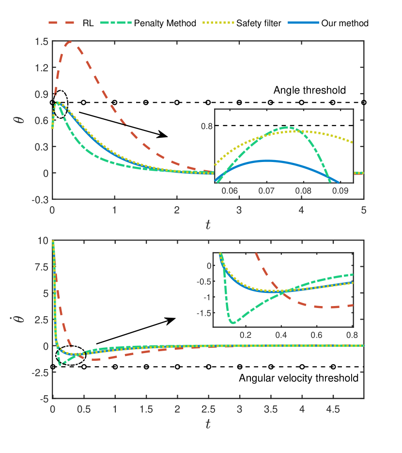
(a)

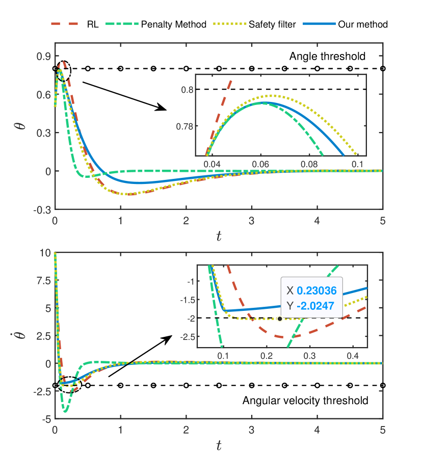
(b)

Figure 3: Trajectories of the angle and angular velocity under four algorithms, i.e., classical RL, RL with penalty term, RL with safety filter and our method. (a) without disturbance/actuator fault; (b) with disturbance/actuator fault

First, we let the disturbance $u^{f}(t)=0$. As shown in Fig.3(a), the classical RL policy will violate the constraint on angle, while all the other three safe learning methods can perform the control task without violating any state constraints.

Then, let the disturbance $u^{f}(t)=-5+0.01\sin(t)+0.03\cos(t)+0.05\sin(2t)+0.04\cos(2t)$. As shown in Fig.3(b), the classical RL policy can stabilize the system under unknown disturbance/actuator fault, but the angle constraint is violated during the learning process. The proposed method in this study can complete the control task while guaranteeing the safety of the system. When the safety filter is introduced into the RL method, the velocity constraint is violated due to $u^{f}$. The control policy learned from the RL method with a CBF-based penalty term cannot keep the velocity trajectory inside the safe region, which may be due to the choice of the penalty term, and the trade-off between the angle constraint and velocity constraint.

Example 5.2.

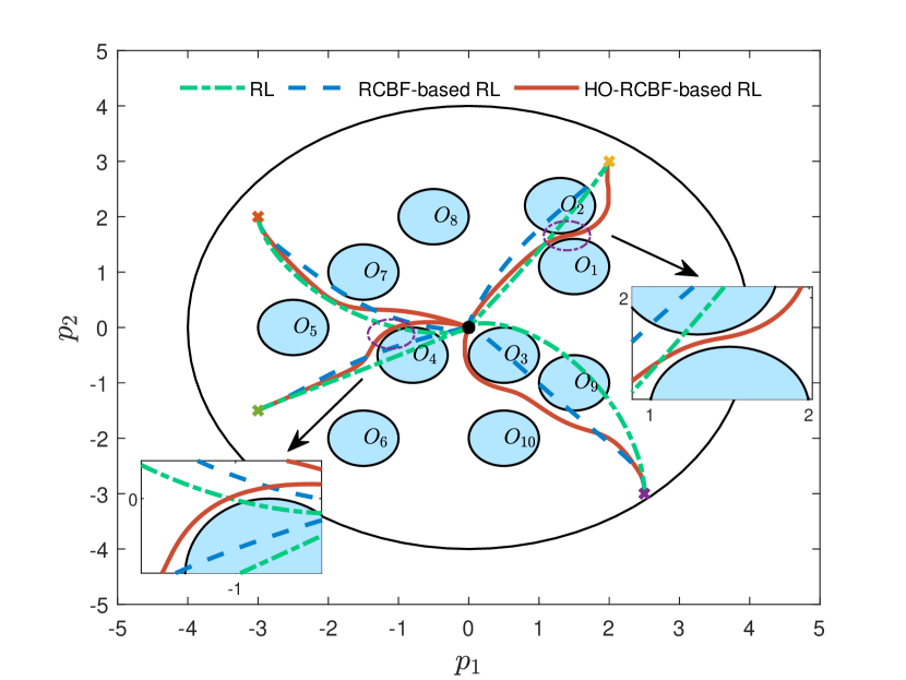
(a)

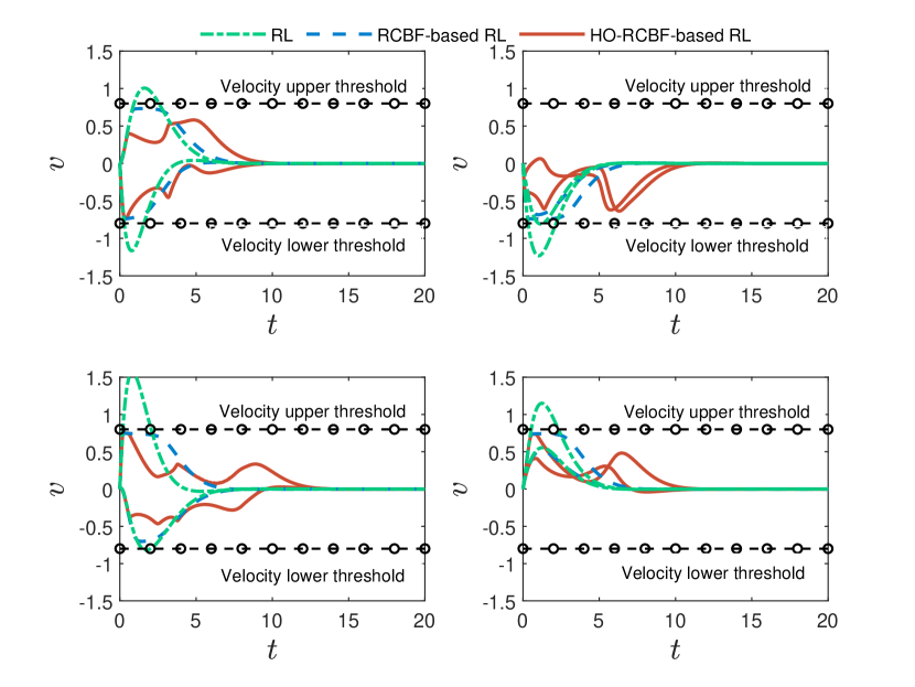
(b)

Figure 4: Position and velocity trajectories of mobile robot under RL, RCBF-based RL [16], HO-RCBF-based RL starting from different initial states.

In this example, the proposed method is shown to handle barrier functions with different relative degrees. We consider a mobile robot described by a double integrator $\dot{p}=v$ and $\dot{v}=u$, where $p=[p_{1},p_{2}]^{\top},v=[v_{1},v_{2}]^{\top}$ and $u\in\mathbb{R}^{2}$ represent the position, the velocity and the input, respectively. The task of the mobile robot is to reach the origin without leaving a circular area centered at the origin while avoiding obstacles and maintaining a defined range of velocity.

Obstacle areas $O_{i}$, $i=1,2,\cdots,N$, are placed randomly inside the circular area, and the collision avoidance constraint for $i_{th}$ obstacle area is given by $\lVert p-c_{i}\rVert^{2}\geq r_{i}^{2}$, where $c_{i}\in\mathbb{R}^{2}$ and $r_{i}\in\mathbb{R}$ are the center and radius of the $i$th obstacle, respectively. The circular area constraint is described as $\lVert p\rVert\leq r^{2}$, where $r\in\mathbb{R}$ is the radius of the area. The constraints on the robot velocity are set to $v_{j,max}\geq v_{j}\geq v_{j,min}$ for $j=1,2$. The position constraint parameter is set to $r=4$\mathrm{m}$$. The speed limit are $v_{1,max}=v_{2,max}=0.8$\mathrm{m}\mathrm{/}\mathrm{s}$$ and $v_{1,min}=v_{2,min}=-0.8$\mathrm{m}\mathrm{/}\mathrm{s}$$.

For the velocity constraint with relative degree one, we define the RCBFs as follows

$$B_{v_{j}}=\frac{1}{h_{v_{j,max}}}+\frac{1}{h_{v_{j,min}}},\ \ \textnormal{for}\ \ j=1,2,$$

where $h_{v_{j,max}}=v_{j,max}-v_{j}$ and $h_{v_{j,min}}=v_{j}-v_{j,min}$. Considering that collision avoidance constraint has relative degree two, we define

$$\psi_{o_{i},0}=h_{o_{i}}, \psi_{o_{i},1}=\dot{\psi}_{o_{i},0}+h_{o_{i}}$$

and the HO-RCBF

$$B_{o_{i}}=\frac{1}{\psi_{o_{i},1}},\ \textnormal{for}\ i=1,2,\cdots,N,$$

where $h_{o_{i}}=\lVert p-c_{i}\rVert^{2}-r_{i}^{2}$. Similarly, for the area constraint, we define

$$\psi_{area,0}=h_{area},\quad\psi_{area,1}=\dot{\psi}_{area,0}+h_{area}$$

and the HO-RCBF $B_{area}=\frac{1}{\psi_{area,1}}$, where $h_{area}=r^{2}-\lVert p\rVert^{2}$. Denote the safeguarding gain for the position constraint as $K_{s,p}$, and the safeguarding gain for the velocity constraint as $K_{s,v}$. The adaptation parameters are selected as $Y=500$ and $\gamma=0.001$, and the initial value of the safeguarding gains are $K_{s,p}(0)=10$ and $K_{s,v}(0)=0.01$. The performance weights are selected as $Q=I$ and $R=I$. The activation functions considered are given by

$$\phi(p,v)=[p_{1}^{2},p_{2}^{2},v_{1}^{2},v_{2}^{2},p_{1}p_{2},p_{1}v_{1},p_{1}v_{2},p_{2}v_{1},p_{2}v_{2},v_{1}v_{2}]^{\top}.$$

The learning gains are set to $k_{c1}=0.1,k_{c2}=1,k_{a1}=100,k_{a2}=1,\beta=0.1$, and the initial weights are $\hat{W}_{c}(0)=\hat{W}_{a}(0)=[40,120,30]$ and $\Gamma(0)=1000I$.

5.0.1 Case 1: the ability to handle constraints with different relative degrees

We compare three algorithms. They include a classical RL, a RCBF-based safe RL [16] and the proposed HO-RCBF-based safe RL. As shown in Fig.4(4(a)) and Fig.4(4(b)), classical RL can find the optimal solution while ignoring both position and velocity constraints. By adding the low-order safeguarding policy to the control policy, the RCBF-based safe RL algorithm can drive the robot to the origin keeping the velocity in the allowable range, while violating the position constraints. Using the proposed HO-RCBF-based safe RL algorithm, the robot can reach the origin without violating either safety constraints. These simulation results show that the proposed method successfully handle constraints of different relative degree.

5.0.2 Case 2: a balance between safety and performance

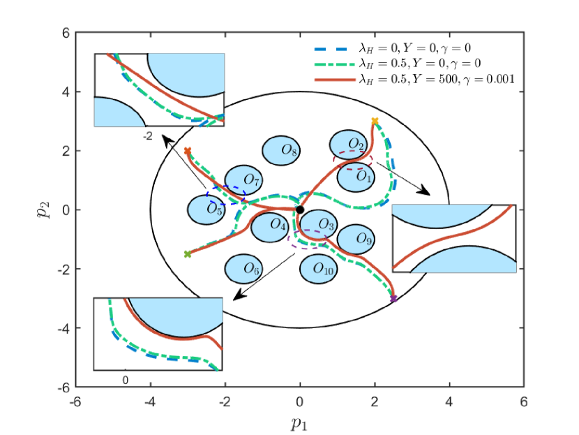
(a)

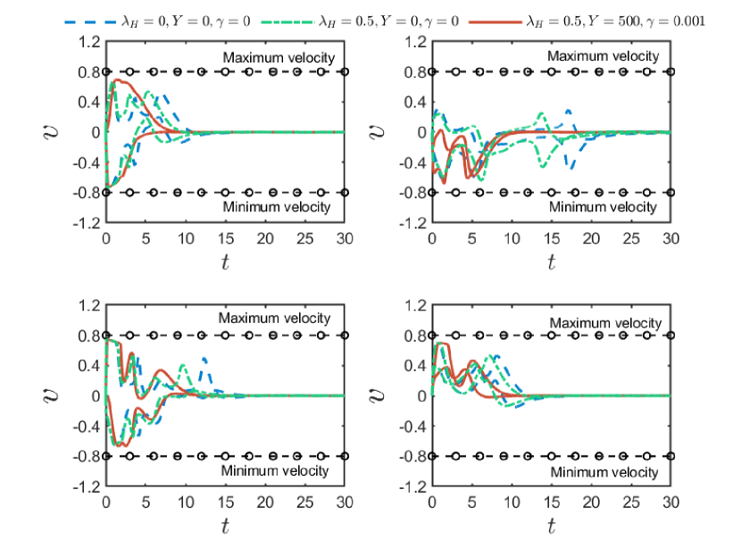
(b)

Figure 5: Position and velocity trajectories of the mobile robot under RL, HO-RCBF-based RL with a constant safeguarding gain, HO-RCBF-based RL with an adaptive safeguarding gain starting from different initial states.

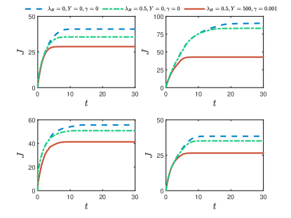
Figure 6: Cost function of the mobile robot under both HO-RBCF-based RL and adaptive HO-RBCF-based RL algorithms with different initial states.

We illustrate the improved performance of the gradient manipulation technique and the adaptive mechanism in the search for the optimal trajectory. To show this, we apply the HO-RCBF-based RL with $\mu=0,\gamma=0,Y=0$, the adaptive HO-RCBF-based RL with $\mu=0.5,\gamma=0,Y=0$, and the adaptive HO-RCBF-based RL with $\mu=0.5,Y=500,\gamma=0.001$. For all methods, $k_{s,v}$ is fixed, and $k_{s,p}$ is updated using the adaptive mechanism. As shown in Fig.5(5(a)) and Fig.5(5(b)), the robot using both the HO-RCBF-based RL algorithm and the adaptive HO-RCBF-based RL algorithm can reach the origin while avoiding all speed and position constraints. However, the position trajectory of the robot using the HO-RCBF-based RL algorithm is more conservative than that the adaptive HO-RCBF-based RL algorithm (see Fig.5(5(a))). Fig.5(5(b)) additionally shows that the robot using the adaptive HO-RCBF-based RL algorithm can reach the target much faster than the HO-RCBF-based RL algorithm. We also consider the energy consumption $J$ required by the robot to perform its task. A higher value of $J$ indicates a greater energy consumption. As shown in Fig.6, given different initial positions $\textnormal{col}(-3,-2),\textnormal{col}(2,3),\textnormal{col}(2.5,-3),\textnormal{col}(-3,-1.5)$, the accumulated cost $J$ of the robot using the adaptive HO-RCBF-based RL algorithm is always significantly less than for the HO-RCBF-based RL algorithm.

6 Conclusion

This paper proposes an adaptive robust safe learning framework that addresses the optimal control problem of nonlinear control systems subject to matching disturbances/faults, while simultaneously addressing optimization and safety requirements. The relationship between optimization and safety is quantified and a balance between these two objectives is achieved. A high-order RCBF is introduced, which can be integrated with RL to address constrained optimal control problems. The proposed safeguarding control policy can handle safety constraints with high relative degree. Interestingly, it can be integrated into any stabilizing control law, designed without considering safety issue, to guarantee the safety of the system.

[]Xinyang Wang received the M.Eng. in Control Engineering from Harbin Institute of Technology, Harbin, China, in 2022. He is currently pursuing the Ph.D. in Control Science and Control Engineering from Harbin Institute of Technology, Shenzhen, China. His current research interests include reinforcement learning, safe learning, game theory and multi-agent systems.

[]Hongwei Zhang received the Ph.D. in mechanical and automation engineering from the Chinese University of Hong Kong in 2010. Subsequently, he held postdoctoral positions with the University of Texas at Arlington, Arlington, TX, USA, and the City University of Hong Kong. From 2012 to 2020, he was with Southwest Jiaotong University, China, and then joined the Harbin Institute of Technology, Shenzhen, China, in 2020, as a Professor. His research interests include cooperative control of multiagent systems, distributed control of microgrids, and active noise control. Dr. Zhang is an Associate Editor for Neurocomputing and Transactions of the Institute of Measurement and Control.

[]Shimin Wang is currently a postdoctoral associate at Massachusetts Institute of Technology where he does research in control theory and machine learning with applications to advanced manufacturing systems. He received a B.Sc. and an M.Eng. from Harbin Engineering University in 2011 and 2014, respectively, and a Ph.D. from The Chinese University of Hong Kong in 2019. He was a recipient of the Best Conference Paper Award at the 2018 IEEE International Conference on Information and Automation and the NSERC Postdoctoral Fellowship award in 2022.

[]Wei Xiao is currently a postdoctoral associate at Massachusetts Institute of Technology. He received a B.Sc. degree from the University of Science and Technology Beijing, China in 2013, a M.Sc. degree from the Chinese Academy of Sciences (Institute of Automation), China in 2016, and a Ph.D. degree from the Boston University, Brookline, MA, USA in 2021. His research interests include control theory and machine learning, with particular emphasis on robotics and traffic control. He received an Outstanding Student Paper Award at the 2020 IEEE Conference on Decision and Control.

[]Martin Guay received a Ph.D. from Queen’s University, Kingston, ON, Canada in 1996. He is currently a Professor in the Department of Chemical Engineering at Queen’s University. His current research interests include nonlinear control systems, especially extremum-seeking control, nonlinear model predictive control, adaptive estimation and control, and geometric control. He was a recipient of the Syncrude Innovation Award, the D. G. Fisher from the Canadian Society of Chemical Engineers, and the Premier Research Excellence Award. He is a Senior Editor of IEEE Transactions on Automatic Control. He is the Editor-in-Chief of the Journal of Process Control. He is also an Associate Editor for Automatica and the Canadian Journal of Chemical Engineering.

References

- [1] A. E. Chriat and C. Sun, “On the optimality, stability, and feasibility of control barrier functions: An adaptive learning-based approach,” IEEE Robotics and Automation Letters, vol. 8, no. 11, pp. 7865–7872, 2023.
- [2] Z. Wang, X. Zhou, C. Xu, and F. Gao, “Geometrically constrained trajectory optimization for multicopters,” IEEE Transactions on Robotics, vol. 38, no. 5, pp. 3259–3278, 2022.
- [3] Z. Cao, S. Xu, X. Jiao, H. Peng, and D. Yang, “Trustworthy safety improvement for autonomous driving using reinforcement learning,” Transportation Research Part C: Emerging Technologies, vol. 138, p. 103656, 2022.
- [4] Y. K. Nakka, A. Liu, G. Shi, A. Anandkumar, Y. Yue, and S.-J. Chung, “Chance-constrained trajectory optimization for safe exploration and learning of nonlinear systems,” IEEE Robotics and Automation Letters, vol. 6, no. 2, pp. 389–396, 2021.
- [5] K. P. Wabersich, A. J. Taylor, J. J. Choi, K. Sreenath, C. J. Tomlin, A. D. Ames, and M. N. Zeilinger, “Data-driven safety filters: Hamilton-Jacobi reachability, control barrier functions, and predictive methods for uncertain systems,” IEEE Control Systems Magazine, vol. 43, no. 5, pp. 137–177, 2023.
- [6] W. Du, J. Ye, J. Gu, J. Li, H. Wei, and G. Wang, “Safelight: A reinforcement learning method toward collision-free traffic signal control,” in Proceedings of the AAAI Conference on Artificial Intelligence, vol. 37, no. 12, 2023, pp. 14 801–14 810.
- [7] M. Selim, A. Alanwar, S. Kousik, G. Gao, M. Pavone, and K. H. Johansson, “Safe reinforcement learning using black-box reachability analysis,” IEEE Robotics and Automation Letters, vol. 7, no. 4, pp. 10 665–10 672, 2022.
- [8] X. He, W. Huang, and C. Lv, “Trustworthy autonomous driving via defense-aware robust reinforcement learning against worst-case observational perturbations,” Transportation Research Part C: Emerging Technologies, vol. 163, p. 104632, 2024.
- [9] A. D. Ames, X. Xu, J. W. Grizzle, and P. Tabuada, “Control barrier function based quadratic programs for safety critical systems,” IEEE Transactions on Automatic Control, vol. 62, no. 8, pp. 3861–3876, 2017.
- [10] S. N. Mahmud, K. Hareland, S. A. Nivison, Z. I. Bell, and R. Kamalapurkar, “A safety aware model-based reinforcement learning framework for systems with uncertainties,” in Proceedings of the American Control Conference, 2021, pp. 1979–1984.
- [11] M. A. Murtaza, S. Aguilera, M. Waqas, and S. Hutchinson, “Safety compliant control for robotic manipulator with task and input constraints,” IEEE Robotics and Automation Letters, vol. 7, no. 4, pp. 10 659–10 664, 2022.
- [12] K. Long, V. Dhiman, M. Leok, J. Cortés, and N. Atanasov, “Safe control synthesis with uncertain dynamics and constraints,” IEEE Robotics and Automation Letters, vol. 7, no. 3, pp. 7295–7302, 2022.
- [13] W. Xiao, C. G. Cassandras, and C. Belta, Safe Autonomy with Control Barrier Functions: Theory and Applications. Springer, 2023.
- [14] Z. Marvi and B. Kiumarsi, “Safe reinforcement learning: A control barrier function optimization approach,” International Journal of Robust and Nonlinear Control, vol. 31, no. 6, pp. 1923–1940, 2021.
- [15] H. Almubarak, E. A. Theodorou, and N. Sadegh, “HJB based optimal safe control using control barrier functions,” in Proceedings of the 60th IEEE Conference on Decision and Control, 2021, pp. 6829–6834.
- [16] M. H. Cohen and C. Belta, “Safe exploration in model-based reinforcement learning using control barrier functions,” Automatica, vol. 147, p. 110684, 2023.
- [17] S. Bandyopadhyay and S. Bhasin, “Safe Q-learning for continuous-time linear systems,” in Proceedings of the 62nd IEEE Conference on Decision and Control, 2023, pp. 241–246.
- [18] M. Li, J. Qin, J. Li, Q. Liu, Y. Shi, and Y. Kang, “Game-based approximate optimal motion planning for safe human-swarm interaction,” IEEE Transactions on Cybernetics, vol. 54, no. 10, pp. 5649–5660, 2024.
- [19] C. Peng, X. Liu, and J. Ma, “Design of safe optimal guidance with obstacle avoidance using control barrier function-based actor–critic reinforcement learning,” IEEE Transactions on Systems, Man, and Cybernetics: Systems, vol. 53, no. 11, pp. 6861–6873, 2023.
- [20] W. Xiao and C. Belta, “High-order control barrier functions,” IEEE Transactions on Automatic Control, vol. 67, no. 7, pp. 3655–3662, 2021.
- [21] S. Gu, B. Sel, Y. Ding, L. Wang, Q. Lin, M. Jin, and A. Knoll, “Balance reward and safety optimization for safe reinforcement learning: A perspective of gradient manipulation,” in Proceedings of the AAAI Conference on Artificial Intelligence, vol. 38, no. 19, 2024, pp. 21 099–21 106.
- [22] H. Xie, L. Dai, Y. Lu, and Y. Xia, “Disturbance rejection MPC framework for input-affine nonlinear systems,” IEEE Transactions on Automatic Control, vol. 67, no. 12, pp. 6595–6610, 2021.
- [23] H.-J. Ma, Y. Liu, T. Li, and G.-H. Yang, “Nonlinear high-gain observer-based diagnosis and compensation for actuator and sensor faults in a quadrotor unmanned aerial vehicle,” IEEE Transactions on Industrial Informatics, vol. 15, no. 1, pp. 550–562, 2019.
- [24] M. Zhai, Q. Sun, B. Wang, R. Wang, Z. Liu, and H. Zhang, “Distributed secondary voltage control of microgrids with actuators bias faults and directed communication topologies: Event-triggered approaches,” International Journal of Robust and Nonlinear Control, vol. 32, no. 7, pp. 4422–4437, 2022.
- [25] Y. Yan, J. Yang, Z. Sun, C. Zhang, S. Li, and H. Yu, “Robust speed regulation for pmsm servo system with multiple sources of disturbances via an augmented disturbance observer,” IEEE/ASME Transactions on Mechatronics, vol. 23, no. 2, pp. 769–780, 2018.
- [26] Z. Peng, J. Wang, and J. Wang, “Constrained control of autonomous underwater vehicles based on command optimization and disturbance estimation,” IEEE Transactions on Industrial Electronics, vol. 66, no. 5, pp. 3627–3635, 2019.
- [27] F. L. Lewis, D. Vrabie, and V. L. Syrmos, Optimal Control. John Wiley & Sons, 2012.
- [28] H. K. Khalil, Nonlinear Systems. NJ: Printice Hall, 2002.
- [29] W. Xiao, T.-H. Wang, R. Hasani, M. Chahine, A. Amini, X. Li, and D. Rus, “Barriernet: Differentiable control barrier functions for learning of safe robot control,” IEEE Transactions on Robotics, vol. 39, no. 3, pp. 2289–2307, 2023.
- [30] L. Wang and J. Dong, “Integral concurrent learning control Lyapunov functions and high order control barrier functions and application to adaptive cruise control,” IEEE Transactions on Intelligent Transportation Systems, vol. 25, no. 5, pp. 3714–3723, 2023.
- [31] X. Kong, W. Ning, Y. Xia, Z. Sun, and H. Xie, “Adaptive high-order control barrier function-based iterative LQR for real time safety-critical motion planning,” IEEE Robotics and Automation Letters, vol. 9, no. 7, pp. 6099–6106, 2024.
- [32] S. Boyd, Convex Optimization. Cambridge UP, 2004.
- [33] W. Xiao, C. Belta, and C. G. Cassandras, “Adaptive control barrier functions,” IEEE Transactions on Automatic Control, vol. 67, no. 5, pp. 2267–2281, 2021.
- [34] P. Ioannou and B. Fidan, Adaptive Control Tutorial. SIAM, 2006.
- [35] F. L. Lewis, S. Jagannathan, and A. Yesildirek, Neural Network Control of Robot Manipulators and Nonlinear Systems. CRC Press, 1998.
- [36] H. Zhang, C. Qin, B. Jiang, and Y. Luo, “Online adaptive policy learning algorithm for state feedback control of unknown affine nonlinear discrete-time systems,” IEEE Transactions on Cybernetics, vol. 44, no. 12, pp. 2706–2718, 2014.
- [37] K. G. Vamvoudakis and F. L. Lewis, “Online actor–critic algorithm to solve the continuous-time infinite horizon optimal control problem,” Automatica, vol. 46, no. 5, pp. 878–888, 2010.
- [38] R. Kamalapurkar, P. Walters, and W. E. Dixon, “Model-based reinforcement learning for approximate optimal regulation,” Automatica, vol. 64, pp. 94–104, 2016.
- [39] R. Kamalapurkar, J. A. Rosenfeld, and W. E. Dixon, “Efficient model-based reinforcement learning for approximate online optimal control,” Automatica, vol. 74, pp. 247–258, 2016.
{IEEEbiography}
[![[Uncaptioned image]](/html/2501.15373/assets/BIO/xywang.jpg) ]Xinyang Wang received the M.Eng. in Control Engineering from Harbin Institute of Technology, Harbin, China, in 2022. He is currently pursuing the Ph.D. in Control Science and Control Engineering from Harbin Institute of Technology, Shenzhen, China. His current research interests include reinforcement learning, safe learning, game theory and multi-agent systems.