Certifying entanglement dimensionality by reduction moments

Abstract

In this paper, we combine the $k$-reduction map, the moment method, and the classical shadow method into a practical protocol for certifying the entanglement dimensionality. Our approach is based on the observation that a state with entanglement dimensionality at most $k$ must stay positive under the action of the $k$-reduction map. The core of our protocol utilizes the moment method to determine whether the $k$-reduced operator, i.e., the operator obtained after applying the $k$-reduction map on a quantum state, contains negative eigenvalues or not. Notably, we propose a systematic method for constructing reduction moment criteria, which apply to a much wider range of states than fidelity-based methods. The performance of our approach gets better and better with the moment order employed, which is corroborated by extensive numerical simulation. To apply our approach, it suffices to implement a unitary 3-design instead of a 4-design, which is more feasible in practice than the correlation matrix method. In the course of study, we show that the $k$-reduction negativity, the absolute sum of the negative eigenvalues of the $k$-reduced operator, is monotonic under local operations and classical communication for pure states.

I Introduction

Entanglement is the characteristic of quantum mechanics and a key resource in quantum information processing [1]. Certification of entanglement is crucial to many practical applications and has been an active research area since the earlier days of quantum information science [2, 3]. In the past 30 years, many entanglement criteria have been proposed, among which the positive partial transpose (PPT) criterion is particularly prominent due to its simplicity and strong capability [4, 5, 6]. However, this criterion requires full information about the density matrix, which is usually not available. To remedy this problem, more practical approaches based on partial transposed moments and randomized measurements were proposed recently [7, 8, 9, 10]. Similar approaches can also be used to estimate Rényi entanglement entropy [11], entanglement entropy [12], and entanglement negativity [13].

For many applications in quantum information processing, including quantum computation and quantum simulation for example, the mere presence of entanglement is usually not enough. Instead we need specific entanglement with desired properties, such as high-dimensional entanglement, which may serve as a benchmark for the potential of a quantum platform. Here the entanglement dimensionality is usually quantified by the Schmidt number [14]. Meanwhile, with the development of quantum technologies, preparation of sophisticated entangled states is no longer a theoretical imagination. Therefore, efficient certification of high-dimensional entanglement is a pressing task [15]. However, this task is very challenging even if the density matrix is known.

A popular tool for certifying entanglement dimensionality are Schmidt-number witnesses [14, 16], which are analogous to entanglement witnesses used for certifying entanglement. Many Schmidt-number witnesses are based on the fidelities with certain target states and are thus useful only when there is sufficient prior information about the states prepared. This requirement is a severe limitation to practical applications. To address this problem, an alternative approach based on the correlation matrix (CM) was proposed recently [17, 18, 19, 20], which does not rely on any target state and has a much wider scope of applications. In addition, the moments of the correlation matrix can be estimated by randomized measurements based on 4-designs. However, 4-designs cannot be realized by discrete groups except for one special case, and most 4-designs known in the literature are not amenable to experimental realization [21, 22, 23].

In this work we propose a practical method for certifying high-dimensional entanglement by combining the $k$-reduction map [14, 24], the moment method [25, 26], and randomized measurements [12, 10]. Our approach is based on the observation that the $k$-reduction map, as a special positive map, preserves the positivity of any density operator with Schmidt number up to $k$, that is, the $k$-reduced operator, the operator obtained after applying the $k$-reduction map is positive. Violation of the positivity condition means the Schmidt number is at least $k+1$. To certify the violation of this condition, we can employ $k$-reduction moments, the moments of the $k$-reduced operator. Moreover, the reduction moments featuring in our approach can be estimated by randomized measurements based on unitary 3-designs, say the Clifford group [27, 28], which is more appealing to experimental realization. If collective measurements are accessible, then these moments can also be estimated more efficiently by permutation tests, which can achieve constant sample complexity.

When the first $2D-1$ moments of the $k$-reduced operator are available for quantum states on a $D$-dimensional Hilbert space, our criterion based on the $k$-reduction moments is equivalent to the $k$-reduction criterion and thus can certify the Schmidt numbers of all pure states. Moreover, the Schmidt numbers of isotropic states can be certified by the third $k$-reduction moment, which represents the lowest nontrivial order. The performances of our criteria are corroborated by extensive numerical calculation in addition to theoretical analysis. In the course of study, we clarify the spectrum of the $k$-reduced operator and introduce the $k$-reduction negativity, the absolute sum of the negative eigenvalues of the $k$-reduced operator, to quantify high-dimensional entanglement. Moreover, we show that the $k$-reduction negativity is Schur concave [29] in the Schmidt spectrum of a pure state and is thus monotonic under local operations and classical communication (LOCC).

The rest of this paper is organized as follows. In Sec. II, we review the definition of Schmidt numbers and give an overview of the correlation matrix method. In Sec. III, we clarify the properties of the $k$-reduction map, $k$-reduction negativity, and $k$-reduction criterion in comparison with the correlation matrix criterion. In Sec. IV, we first review the basic idea of the moment method and then propose our certification criteria based on $k$-reduction moments. In Sec. V, we illustrate the performances of our certification criteria based on numerical simulation. In Sec. VI, we present two methods for estimating reduction moments and discuss the sample complexities. Finally, we make the conclusions in Sec. VII. A summary of main results is presented in Table 1. Some technical proofs are relegated to the Appendices.

Table 1: Comparison between different Schmidt number certification protocols for quantum states with total dimension $D$.

Method	Require knowledge about the target state	Order of unitary design	Sample complexity
Fidelity-based [16]	Yes	/	$\mathcal{O}(1)$
Correlation matrix [18, 19]	No	$\geq 4$	Unknown
Full state tomography of rank-$r$ states [30]	No	4	$\mathcal{O}(D^{2}r)$
Moments of $k$-reduced operator (This work)	No	$\geq 3$	$\mathcal{O}(D)$ Appendix E

II Background

Given a finite-dimensional Hilbert space $\mathcal{H}$, denote by $\mathcal{L}(\mathcal{H})$, $\mathcal{L}^{\mathrm{H}}(\mathcal{H})$, and $\mathcal{L}_{0}^{\mathrm{H}}(\mathcal{H})$ the set of linear operators, the set of Hermitian operators, and the set of traceless Hermitian operators on $\mathcal{H}$, respectively. The spectrum (with multiplicities taken into account) and the minimum eigenvalue of a Hermitian operator $O$ are denoted by $\sigma(O)$ and $\sigma_{\min}(O)$, respectively.

II.1 Schmidt number

Consider a bipartite system with Hilbert space $\mathcal{H}_{AB}=\mathcal{H}_{A}\otimes\mathcal{H}_{B}$. Let $d_{A}\equiv\dim(\mathcal{H}_{A})$, $d_{B}\equiv\dim(\mathcal{H}_{B})$, $D\equiv d_{A}d_{B}$, and $d\equiv\min\{d_{A},d_{B}\}$. Without loss of generality, we assume $d_{A}\leq d_{B}$ throughout this paper, which means $d=d_{A}$. The Schmidt number (also known as Schmidt rank) of a pure state $|\psi\rangle$ in $\mathcal{H}_{AB}$ is defined as

$$\mathrm{SN}(|\psi\rangle)\equiv\mathrm{rank}(\rho_{A}),$$ (1)

where $\rho_{A}=\Tr_{B}(|\psi\rangle\langle\psi|)$. Note that $\mathrm{SN}(|\psi\rangle)=1$ iff $|\psi\rangle$ is a product state. The Schmidt spectrum of $|\psi\rangle$, denoted by $\sigma(\psi)$, is the set of eigenvalues of $\rho_{A}$ (with multiplicities taken into account) [31], that is, $\sigma(\psi)\equiv\sigma(\rho_{A})$. If $|\psi\rangle$ has Schmidt decomposition

$$|\psi\rangle=\sum_{i=0}^{d-1}\sqrt{\lambda_{i}}|i\rangle_{A}\otimes|i\rangle_{B},$$ (2)

then its Schmidt spectrum reads $\sigma(\psi)=\{\lambda_{i}\}_{i=0}^{d-1}$. In addition, the vector $\boldsymbol{\lambda}=(\lambda_{0},\lambda_{1},\ldots,\lambda_{d-1})$ is called the Schmidt vector of $|\psi\rangle$. This vector can be regarded as a point on the $(d-1)$-dimensional probability simplex

$$\!\!\Delta_{d}\equiv\left\{(x_{0},x_{1},\ldots,x_{d-1}):\sum_{i=0}^{d-1}x_{i}=1,x_{i}\geq 0\right\}.$$ (3)

If $\lambda_{0}=\cdots=\lambda_{r-1}=1/r$ and $\lambda_{r}=\cdots=\lambda_{d-1}=0$, then we get the maximally entangled state with Schmidt number $r$,

$$|+_{r}\rangle\equiv\frac{1}{\sqrt{r}}\sum_{i=0}^{r-1}|i\rangle_{A}\otimes|i\rangle_{B}.$$ (4)

The concept of Schmidt number can also be generalized to mixed states. Denote by $\mathcal{S}_{r}$ the set of quantum states on $\mathcal{H}_{AB}$ that can be expressed as convex combinations of pure states with Schmidt numbers no larger than $r$. By definition we have the following hierarchy relation

$$\mathcal{S}_{1}\subset\mathcal{S}_{2}\subset\cdots\subset\mathcal{S}_{d}=\mathcal{S}(\mathcal{H}_{AB}),$$ (5)

where $\mathcal{S}(\mathcal{H}_{AB})$ denotes the set of all density operators on $\mathcal{H}_{AB}$. The Schmidt number $\mathrm{SN}(\rho)$ of $\rho\in\mathcal{S}(\mathcal{H}_{AB})$ is defined as the smallest integer $r$ such that $\rho\in\mathcal{S}_{r}$. Alternatively, $\mathrm{SN}(\rho)$ can be expressed as follows [14],

$$\mathrm{SN}(\rho)\equiv\min_{\mathbb{D}(\rho)}\max_{\phi_{i}\in\mathbb{D}(\rho)}\mathrm{SN}(\ket{\phi_{i}}),$$ (6)

where $\mathbb{D}(\rho)$ denotes a pure-state decomposition of $\rho$. A quantum state with Schmidt number $r$ can be prepared from $|+_{r}\rangle$ using LOCC, but cannot be prepared from any state with a lower Schmidt rank. Hence, the Schmidt number of a mixed state $\rho$ quantifies its entanglement dimension.

II.2 Schmidt number certification via the correlation matrix

Here we review the correlation matrix method for certifying Schmidt numbers [17, 18, 19], assuming that $d_{A}=d_{B}=d$. Let $\{P^{(A)}_{i}\}_{i=1}^{d^{2}-1}$ and $\{P^{(B)}_{i}\}_{i=1}^{d^{2}-1}$ be orthogonal operator bases of $\mathcal{L}_{0}^{\mathrm{H}}(\mathcal{H}_{A})$ and $\mathcal{L}_{0}^{\mathrm{H}}(\mathcal{H}_{B})$, respectively, that satisfy the conditions

$$\Tr(P^{(A)}_{i}) =\Tr(P^{(B)}_{i})=0,$$ (7)

$$\Tr(P^{(A)}_{i}P^{(A)}_{j}) =\Tr(P^{(B)}_{i}P^{(B)}_{j})=d\delta_{i,j}.$$

The correlation matrix $T$ of $\rho$ with respect to these bases is the $(d^{2}-1)\times(d^{2}-1)$ matrix with entries

$$T_{ij}\equiv\frac{1}{d}\Tr\left[\rho\left(P^{(A)}_{i}\otimes P^{(B)}_{j}\right)\right].$$ (8)

Suppose $T$ has singular values $\{v_{i}\}_{i=1}^{d^{2}-1}$; then its Schatten $p$-norm reads

$$\|T\|_{p}\equiv\left(\sum_{i=1}^{d^{2}-1}v_{i}^{p}\right)^{\frac{1}{p}}=\left\{\Tr[(TT^{\top})^{\frac{p}{2}}\Bigr{]}\right\}^{\frac{1}{p}}.$$ (9)

The correlation matrix criterion states that [18, 19]

$$\text{ if }\mathrm{SN}(\rho)\leq k,\text{ then }\|T\|_{1}\leq k-\frac{1}{d}.$$ (10)

Note that this criterion is independent of the specific choices of local operator bases. If the second inequality in Eq. (10) is violated, then we can conclude that $\mathrm{SN}(\rho)$ is larger than $k$.

In practice, it is very difficult to estimate the singular values of $T$ and the 1-norm $\|T\|_{1}$. Nevertheless, the second and fourth moments of the singular values, that is, $(\|T\|_{2}^{2},\|T\|_{4}^{4})$, can be estimated from the second and fourth order Haar-randomized correlators $\mathcal{C}^{(n)}$ based on a special observable $O$,

$$\!\!\!\mathcal{C}^{(n)}\equiv\int dU_{A}dU_{B}\left\{\Tr[\rho(U_{A}OU_{A}^{\dagger}\otimes U_{B}OU_{B}^{\dagger})]\right\}^{n}.$$ (11)

More precisely, we have the following relations [18, 19],

$$\mathcal{C}^{(2)} =\frac{d^{2}}{(d-1)^{2}}\|T\|_{2}^{2},$$ (12)

$$\mathcal{C}^{(4)} =\frac{2d^{4}}{3(d-1)^{4}}\|T\|_{4}^{4}+\frac{1}{3}(\mathcal{C}^{(2)})^{2}.$$

Define the region

$$\mathcal{T}_{k}\equiv\left\{(\|T\|_{2}^{2},\|T\|_{4}^{4}):\|T\|_{1}\leq k-d^{-1}\right\},$$ (13)

whose boundary can be determined by solving an optimization problem. Then a moment-based correlation matrix criterion can be formulated as follows,

$$\text{ if }\mathrm{SN}(\rho)\leq k,\text{ then }(\|T\|_{2}^{2},\|T\|_{4}^{4})\in\mathcal{T}_{k}.$$ (14)

This criterion is referred to as the moment-based CM criterion henceforth.

In addition, by virtue of the Hölder inequality we can deduce that

$$\|T\|_{2}^{2} =\sum_{i=1}^{d^{2}-1}v_{i}^{2/3}v_{i}^{4/3}\leq\left(\sum_{i=1}^{d^{2}-1}v_{i}\right)^{2/3}\left(\sum_{i=1}^{d^{2}-1}v_{i}^{4}\right)^{1/3}$$

$$=\|T\|_{1}^{2/3}\|T\|_{4}^{4/3},$$ (15)

which implies that

$$\|T\|_{1}\geq\frac{\|T\|_{2}^{3}}{\|T\|_{4}^{2}}.$$ (16)

In conjunction with Eq. (10) we can deduce an alternative moment-based criterion

$$\text{ if }\mathrm{SN}(\rho)\leq k,\text{ then }\frac{\|T\|_{2}^{3}}{\|T\|_{4}^{2}}\leq k-\frac{1}{d},$$ (17)

which is potentially weaker but simpler than the counterpart in Eq. (14).

Currently, it is still quite challenging to apply the moment-based criteria in real experiments, although it is easier than the original correlation matrix criterion. To estimate the fourth order correlator $\mathcal{C}^{(4)}$ experimentally, we need to implement unitary transformations in a unitary $4$-design. Unfortunately, the Clifford group widely used in quantum information processing fails to be a unitary $4$-design [27, 28, 22], and it is very challenging to sample from a unitary 4-design in experiments. Therefore, it is desirable to construct alternative certification protocols that do not rely on unitary 4-designs, which is a main motivation behind the current work.

III Schmidt number certification via the $k$-reduction map

III.1 $k$-positive maps

Given a finite-dimensional Hilbert space $\mathcal{H}$, an operator $X\in\mathcal{L}(\mathcal{H})$ is positive (semidefinite), denoted as $X\geq 0$, if $\langle\psi|X|\psi\rangle\geq 0$ for all $|\psi\rangle\in\mathcal{H}$. A linear map $\mathcal{M}:\mathcal{L}(\mathcal{H})\to\mathcal{L}(\mathcal{H})$ is positive if

$$\mathcal{M}(X)\geq 0\quad\forall X\geq 0.$$ (18)

A linear map $\mathcal{M}:\mathcal{L}(\mathcal{H})\to\mathcal{L}(\mathcal{H})$ is $k$-positive if the map $\mathcal{I}_{k}\otimes\mathcal{M}$ is positive, where $\mathcal{I}_{k}$ is the identity map on an auxiliary Hilbert space of dimension $k$ [32, 33, 34, 35].

Next, we turn to a bipartite system with Hilbert space $\mathcal{H}_{AB}=\mathcal{H}_{A}\otimes\mathcal{H}_{B}$ and explain the applications of $k$-positive maps in certifying high-dimensional entanglement. Let $\mathcal{I}_{A}$ be the identity map on $\mathcal{L}(\mathcal{H}_{A})$. A linear map $\mathcal{M}$ on $\mathcal{L}(\mathcal{H}_{B})$ is $k$-positive iff $\mathcal{I}_{A}\otimes\mathcal{M}(|\psi\rangle\langle\psi|)$ is positive for every pure state $|\psi\rangle\in\mathcal{H}_{AB}$ with $\mathrm{SN}(\psi)\leq k$ [14, 36]. Then we also have $\mathcal{I}_{A}\otimes\mathcal{M}(\rho)\geq 0$ for every mixed state $\rho$ with $\mathrm{SN}(\rho)\leq k$, but the converse is not necessarily true. Therefore, if $\mathcal{I}_{A}\otimes\mathcal{M}(\rho)$ is not positive, then we can conclude that $\mathrm{SN}(\rho)>k$. This fact is instrumental to constructing protocols for certifying high-dimensional entanglement.

III.2 $k$-reduction map and $k$-reduction criterion

One of the most important and common $k$-positive maps is the $k$-reduction map [33, 34], which is defined as follows,

$$\mathcal{R}_{k}(X)\equiv k\Tr(X)I-X.$$ (19)

Here we are mainly interested in the map $\mathcal{I}_{A}\otimes\mathcal{R}_{k}$ acting on $\mathcal{L}(\mathcal{H}_{\mathrm{A}}\otimes\mathcal{H}_{B})$. To simplify the following discussion, the expression $\mathcal{I}_{A}\otimes\mathcal{R}_{k}(\rho)$ will be abbreviated as $\mathcal{R}_{k}(\rho)$ and called the $k$-reduced operator associated with $\rho$. When $\rho=|\psi\rangle\langle\psi|$ is a pure state, $\mathcal{R}_{k}(\rho)$ can further be abbreviated as $\mathcal{R}_{k}(\psi)$. Our approach for certifying the Schmidt number is based on the following well-known result [14]:

Proposition 1.

If $\mathrm{SN}(\rho)\leq k$, then

$$\mathcal{R}_{k}(\rho)=k\rho_{A}\otimes I_{B}-\rho\geq 0.$$ (20)

When $\rho$ is a pure state, the condition $\mathrm{SN}(\rho)\leq k$ is also necessary to guarantee Eq. (20).

If the condition in Eq. (20), known as the $k$-reduction condition, is violated, then we can conclude that $\text{SN}(\rho)>k$. The basic idea of this criterion is analogous to the famous PPT criterion. By considering the expectation value of the $k$-reduced operator with respect to the maximally entangled state $|+_{d}\rangle$ we can deduce that

$$\text{if }\mathrm{SN}(\rho)\leq k,\quad\text{ then }\langle+_{d}|\rho|+_{d}\rangle\leq\frac{k}{d},$$ (21)

which reproduces a fidelity-based criterion.

In analogy to the entanglement negativity [36], here we define the $k$-reduction negativity of $\rho$, denoted by $\mathcal{N}_{k}(\rho)$, as the absolute value of the sum of the negative eigenvalues of $\mathcal{R}_{k}(\rho)$. When $\rho=|\psi\rangle\langle\psi|$ is a pure state, $\mathcal{N}_{k}(\rho)$ is abbreviated as $\mathcal{N}_{k}(\psi)$. Alternatively, $\mathcal{N}_{k}(\rho)$ can be expressed as follows,

$$\mathcal{N}_{k}(\rho) =\frac{1}{2}\left(\|\mathcal{R}_{k}(\rho)\|_{1}-\Tr[\mathcal{R}_{k}(\rho)]\right)$$

$$=\frac{1}{2}\left(\|\mathcal{R}_{k}(\rho)\|_{1}-kd_{B}+1\right).$$ (22)

It measures the degree to which the $k$-reduction criterion is violated. With this definition, the $k$-reduction criterion can also be formulated as follows,

$$\text{if }\mathrm{SN}(\rho)\leq k,\quad\text{ then }\mathcal{N}_{k}(\rho)=0.$$ (23)

In other words, if $\mathcal{N}_{k}(\rho)>0$, then we can deduce that $\mathrm{SN}(\rho)>k$.

III.3 $k$-reduction negativity of pure states

The $k$-reduction negativity plays an important role in certifying high-dimensional entanglement as we have seen in Sec. III.2. Here we determine the $k$-reduction negativity of a general bipartite pure state $|\psi\rangle$ in $\mathcal{H}_{AB}$ and clarify its basic properties. To this end, we need to introduce some additional notations and results.

Given two real vectors $\mathbf{x}$ and $\mathbf{y}$ in $\mathbb{R}^{d}$, we can rearrange the entries of each vector in nonincreasing order to obtain $\mathbf{x}^{\downarrow}=(x^{\prime}_{0},x^{\prime}_{1},\ldots,x^{\prime}_{d-1})$ and $\mathbf{y}^{\downarrow}=(y^{\prime}_{0},y^{\prime}_{1},\ldots,y^{\prime}_{d-1})$. If

$$\sum_{i=0}^{\ell-1}x^{\prime}_{i}\geq\sum_{i=0}^{\ell-1}y^{\prime}_{i}\quad\forall\ell,$$ (24)

and the inequality is saturated when $\ell=d$, then we say $\mathbf{x}$ majorizes $\mathbf{y}$, denoted by $\mathbf{x}\succ\mathbf{y}$ or $\mathbf{y}\prec\mathbf{x}$. A function $F$ on a subset of $\mathbb{R}^{d}$ is Schur concave if the condition $\mathbf{x}\succ\mathbf{y}$ implies that $F(\mathbf{x})\leq F(\mathbf{y})$ [29, 31].

Given $\boldsymbol{\lambda}\in\Delta_{d}$, let $\Omega_{k}(\boldsymbol{\lambda})$ be the $d\times d$ matrix with entries

$$\Omega_{k}(\boldsymbol{\lambda})_{ij}=k\lambda_{i}\delta_{ij}-\sqrt{\lambda_{i}\lambda_{j}}$$ (25)

and define

$$\theta_{k}(\boldsymbol{\lambda})\equiv\max\{0,-\sigma_{\min}(\Omega_{k}(\boldsymbol{\lambda}))\}.$$ (26)

This function is interesting because of its close relation with the $k$-reduction negativity as we shall see shortly. The basic properties of $\Omega_{k}(\boldsymbol{\lambda})$ and $\theta_{k}(\boldsymbol{\lambda})$ are summarized in Lemmas 2 and 3 in Appendix A.

Now, we can clarify the basic properties of the $k$-reduced operator $\mathcal{R}_{k}(\psi)$ as summarized in the following theorem and proved in Appendix A. Part of the results has been proved in previous works [34, 14].

Theorem 1.

Suppose $|\psi\rangle\in\mathcal{H}_{AB}$ is a pure state with Schmidt vector $\boldsymbol{\lambda}$, Schmidt number $r$, and $\tilde{r}$ distinct nonzero Schmidt coefficients. Then the $k$-reduced operator $\mathcal{R}_{k}(\psi)$ has spectrum

$$\sigma(\mathcal{R}_{k}(\psi)) =\sigma(\Omega_{k}(\boldsymbol{\lambda}))\cup[k\sigma(\psi)]^{\times(d_{B}-1)},$$ (27)

where the superscript $d_{B}-1$ denotes the multiplicity. In addition, $\mathcal{R}_{k}(\psi)$ has $2\tilde{r}$ distinct nonzero eigenvalues when $k\neq r$ and $2\tilde{r}-1$ distinct nonzero eigenvalues when $k=r$. If $k\geq r$, then $\Omega_{k}(\boldsymbol{\lambda})\geq 0$ and $\mathcal{R}_{k}(\psi)\geq 0$. If instead $1\leq k<r$, then both $\Omega_{k}(\boldsymbol{\lambda})$ and $\mathcal{R}_{k}(\psi)$ have exactly one negative eigenvalue.

Theorem 1 implies that

$$\mathcal{N}_{k}(\psi)=\max\{0,-\sigma_{\min}(\mathcal{R}_{k}(\psi))\}=\theta_{k}(\boldsymbol{\lambda}).$$ (28)

In conjunction with Lemma 2 in Appendix A, we can further clarify the properties of $\mathcal{N}_{k}(\psi)$. The following theorem is also proved in Appendix A.

Theorem 2.

Suppose $|\psi\rangle\in\mathcal{H}_{AB}$ is a pure state with Schmidt vector $\boldsymbol{\lambda}$. Then $\theta_{k}(\boldsymbol{\lambda})$ is Schur concave in $\boldsymbol{\lambda}$ and nonincreasing with $k$. If $\mathrm{SN}(\psi)=r$, then $\mathcal{N}_{k}(\psi)\leq 1-k/r$, and the inequality is saturated when $|\psi\rangle$ is a maximally entangled state with $\mathrm{SN}(\psi)=r$.

Suppose $|\psi\rangle$ and $|\psi^{\prime}\rangle$ are two pure states in $\mathcal{H}_{AB}$. According to Nielsen’s majorization criterion [37], $|\psi\rangle$ can be transformed into $|\psi^{\prime}\rangle$ under LOCC iff the Schmidt vector of $|\psi\rangle$ is majorized by that of $|\psi^{\prime}\rangle$. In conjunction with Theorem 2, we can deduce that the $k$-reduction negativity is nonincreasing under LOCC and thus can serve as a high-dimensional entanglement monotone for pure states.

By virtue of Theorem 2 we can further derive tight bounds on the $k$-reduction negativity $\mathcal{N}_{k}(\rho)$ and eigenvalues of $\mathcal{R}_{k}(\rho)$ for a general mixed state $\rho$.

Corollary 1.

Suppose $\rho\in\mathcal{S}(\mathcal{H}_{AB})$ with $d_{A}=d_{B}=d$. Then

$$\mathcal{N}_{k}(\rho)\leq 1-\frac{k}{d},\quad\left(\frac{k}{d}-1\right)I\leq\mathcal{R}_{k}(\rho)\leq kI.$$ (29)

III.4 $k$-reduction negativity of pure states with depolarizing noise

As a generalization, in this section we determine the $k$-reduction negativity of an arbitrary pure state with depolarizing noise. Suppose $|\psi\rangle\in\mathcal{H}_{AB}$ is a pure state with $\mathrm{SN}(\psi)=r$ and $\rho$ has the form

$$\rho=(1-\varepsilon)|\psi\rangle\langle\psi|+\varepsilon\frac{I}{d_{A}d_{B}},\quad\varepsilon\in[0,1].$$ (30)

Then

$$\mathcal{R}_{k}(\rho) =(1-\varepsilon)\mathcal{R}_{k}(\psi)+\varepsilon\mathcal{R}_{k}\left(\frac{I}{d_{A}d_{B}}\right)$$

$$=(1-\varepsilon)\mathcal{R}_{k}(\psi)+\frac{\varepsilon(kd_{B}-1)}{d_{A}d_{B}}I,$$ (31)

and there exists a simple linear relation between the spectrum of $\mathcal{R}_{k}(\rho)$ and the spectrum of $\mathcal{R}_{k}(\psi)$. Notably, we have

$$\sigma_{\min}(\mathcal{R}_{k}(\rho))=(1-\varepsilon)\sigma_{\min}(\mathcal{R}_{k}(\psi))+\frac{\varepsilon(kd_{B}-1)}{d_{A}d_{B}}.$$ (32)

In conjunction with Theorems 1 and 2, it is now straightforward to deduce the following result.

Proposition 2.

The $k$-reduction negativity of $\rho$ in Eq. (30) reads

$$\mathcal{N}_{k}(\rho)=\begin{cases}0,&\varepsilon\geq\varepsilon^{*},\\ (1-\varepsilon)\mathcal{N}_{k}(\psi)-\frac{\varepsilon(d_{B}k-1)}{d_{A}d_{B}},&\varepsilon<\varepsilon^{*},\end{cases}$$ (33)

where

$$\varepsilon^{*}\equiv\frac{d_{A}d_{B}\mathcal{N}_{k}(\psi)}{kd_{B}-1+d_{A}d_{B}\mathcal{N}_{k}(\psi)}.$$ (34)

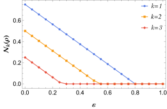
Figure 1: The $k$-reduction negativity $\mathcal{N}_{k}(\rho_{\varepsilon,r})$ as a function of $\varepsilon$ for $k=1,2,3$. Here we set $r=d_{A}=d_{B}=4$. The $k$-reduction negativity is nonincreasing in $k$ and $\varepsilon$ as expected.

Next, we turn to the special case in which $|\psi\rangle$ is a maximally entangled state of Schmidt rank $r$. Define

$$\rho_{\varepsilon,r}\equiv(1-\varepsilon)|+_{r}\rangle\langle+_{r}|+\varepsilon\frac{I}{d_{A}d_{B}},\quad\varepsilon\in[0,1].$$ (35)

The dependence of $\mathcal{N}_{k}(\rho_{\varepsilon,r})$ on $k$ and $\varepsilon$ is illustrated in Fig. 1. Define $\varepsilon_{c}^{(\mathrm{RM})}$ as the minimum value of of $\varepsilon\geq 0$ such that $\mathcal{N}_{r-1}(\rho_{\varepsilon,r})=0$. By virtue of Proposition 2 with $\mathcal{N}_{r-1}(+_{r})=1/r$ we can deduce that

$$\varepsilon_{c}^{(\mathrm{RM})}=\left(1+\frac{r^{2}-r}{d_{A}}-\frac{r}{d_{A}d_{B}}\right)^{-1}.$$ (36)

As the local dimensions $d_{A},d_{B}$ increase, $\varepsilon_{c}^{(\mathrm{RM})}$ approaches 1, so the $k$-reduction criterion can certify the Schmidt number of $\rho_{\varepsilon,r}$ with arbitrary noise strength asymptotically.

Using the $k$-reduction criterion, we can further derive the following informative lower and upper bounds for the Schmidt number of $\rho_{\varepsilon,r}$ as proved in Appendix A.4.

Proposition 3.

The Schmidt number of $\rho_{\varepsilon,r}$ in Eq. (35) satisfies

$$\left\lceil\frac{(1+u)r}{1+d_{B}ru}\right\rceil\leq\mathrm{SN}(\rho_{\varepsilon,r})\leq\left\lceil\frac{(1+u)r}{1+r^{2}u}\right\rceil,$$ (37)

where $u=\varepsilon/[(1-\varepsilon)d_{A}d_{B}]$. If $r\leq\sqrt{d_{A}}$ and $\varepsilon<1/2$, then $\mathrm{SN}(\rho_{\varepsilon,r})=r$.

III.5 Comparison with the correlation matrix criterion

In this section we compare the $k$-reduction criterion in Eq. (20) with the correlation matrix criterion in Eq. (10) under various situations. From Proposition 1, we know that the $k$-reduction criterion can certify the Schmidt number of any pure state. By contrast, the correlation matrix criterion cannot. For example, consider the following state with Schmidt rank $r=4$,

$$\sqrt{\frac{4}{5}}|00\rangle+\sqrt{\frac{1}{15}}|11\rangle+\sqrt{\frac{1}{15}}|22\rangle+\sqrt{\frac{1}{15}}|33\rangle,$$ (38)

assuming that $d_{A}=d_{B}=d=4$. The 1-norm of its correlation matrix is approximately 2.7231, which is smaller than the upper bound $r-1-d^{-1}=11/4$ in Eq. (10) with $k=r-1$. Thus, from the correlation matrix criterion, we can only conclude that its Schmidt number is at least 3, instead of the actual Schmidt number $4$.

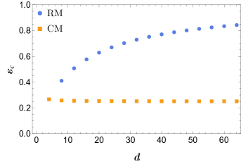
Figure 2: Noise thresholds $\varepsilon^{(\mathrm{RM})}_{c}$ and $\varepsilon^{(\mathrm{CM})}_{c}$ associated with the $k$-reduction criterion and correlation matrix criterion in certifying the Schmidt number of the state $\rho_{\varepsilon,r}$ in Eq. (35) with $r=4$. Here $d_{A}=d_{B}=d$, and $\varepsilon^{(\mathrm{RM})}_{c}$ is given in Eq. (36).

Next, we consider the state $\rho_{\varepsilon,r}$ defined in Eq. (35). According to the discussion in Sec. III.4, the $k$-reduction criterion can certify that the Schmidt number of $\rho_{\varepsilon,r}$ is $r$ when $\varepsilon$ is smaller than the threshold $\varepsilon^{(\mathrm{RM})}_{c}$ in Eq. (36). As an analogy, we define $\varepsilon^{(\mathrm{CM})}_{c}$ as the maximum value of $\varepsilon$ satisfying $\|T\|_{1}\geq r-1-d^{-1}$. The relations between the two parameters and the local dimension $d$ are illustrated in Fig. 2, which implies that the $k$-reduction criterion can tolerate much higher noise strength than the correlation matrix criterion.

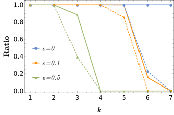
Figure 3: Detection ratios of the $k$-reduction criterion and correlation matrix criterion for the ensemble of states in Eq. (39). The solid lines correspond to the $k$-reduction criterion in Eq. (20), while the dashed lines correspond to the correlation matrix criterion in Eq. (10). Here $d_{A}=d_{B}=8$ and three different noise strengths are shown in the legend. The performances of the $k$-reduction criterion are better than the correlation matrix criterion in all cases under consideration.

We then consider Haar random pure states with depolarizing noise. Define the ensemble

$$\mathcal{E}_{\mathrm{Haar},\varepsilon}\equiv\left\{(1-\varepsilon)U|0\rangle\langle 0|U^{\dagger}+\varepsilon\frac{I}{d^{2}}:U\sim\mathrm{Haar}\right\},$$ (39)

where $|0\rangle\in\mathcal{H}_{AB}$, $d_{A}=d_{B}=d$, and $0\leq\varepsilon\leq 1$. When $\varepsilon$ is sufficiently small, a random sample $\rho$ from this ensemble almost surely has the maximum Schmidt number, that is, $\mathrm{SN}(\rho)=d$. To compare the performances of the $k$-reduction criterion and correlation matrix criterion, Fig. 3 illustrates their detection ratios determined by numerical simulation as functions of $k$ for three different noise strengths $\varepsilon$. Here the detection ratio of a criterion denotes the percentage of quantum states in a given ensemble that is certified to have $\mathrm{SN}(\rho)>k$ by this criterion. The $k$-reduction criterion has higher detection ratios than the correlation matrix criterion in all cases under consideration. In other words, the $k$-reduction criterion is more effective in certifying the Schmidt numbers of pure states with depolarizing noise.

Finally, we consider random mixed states with induced measures [38]. Let $\mathcal{H}_{C}$ be a $K$-dimensional Hilbert space. Denote by $\mathcal{E}_{D,K}$ the ensemble of mixed states on $\mathcal{H}_{AB}$ induced by Haar random pure states on $\mathcal{H}_{AB}\otimes\mathcal{H}_{C}$. Tables 3 and 3 summarize the detection ratios of the $k$-reduction criterion and correlation matrix criterion for various choices of the parameters $K$ and $k$ as determined by numerical simulation with $d_{A}=d_{B}=16$. According to the two tables, the correlation matrix criterion is stronger than the $k$-reduction criterion for large $K$, in which case the states in the ensemble $\mathcal{E}_{D,K}$ tend to have low purities. In the special case $K=2$, the two criteria have comparable performances: both of them can certify that almost all states in the ensemble $\mathcal{E}_{256,2}$ have Schmidt numbers at least $8$.

Table 2: Detection ratio of the $k$-reduction criterion in Eq. (20) for the ensemble $\mathcal{E}_{256,K}$. Here $d_{A}=d_{B}=16$.

	2	3	4	5	6
2	1	1	1	1	1
3	1	1	1	1	0.9976
4	1	1	1	0.0176	0
5	1	1	0.0006	0	0
6	1	0.1596	0	0	0
7	1	0	0	0	0
8	1	0	0	0	0
9	0.0022	0	0	0	0

Table 3: Detection ratio of the correlation matrix criterion in Eq. (10) for the ensemble $\mathcal{E}_{256,K}$. Here $d_{A}=d_{B}=16$.

	2	3	4	5	6
5	1	1	1	1	1
6	1	1	1	0	0
7	1	1	0	0	0
8	1	0	0	0	0
9	0.0034	0	0	0	0

IV Schmidt number certification via $k$-reduction moments

In this section we systematically develop the moment method, which is designed to characterize the subset of positive operators within a given set of Hermitian operators, and apply this method to certifying the Schmidt number.

IV.1 PT moments and $k$-reduction moments

Here we give an overview of how the moment method is utilized in entanglement certification [7].

The well-known PPT criterion states that if the partial transpose $\rho^{\top}$ (with respect to either party) of a bipartite state $\rho$ is not a positive operator, then $\rho$ is necessarily entangled. This criterion is proved to be useful for a large class of quantum states. However, non-complete positive maps, including the partial transpose and $k$-reduction map, are non-physical. We cannot implement them directly in the laboratory. One solution to this problem is quantum tomography. After reconstructing the entire density matrix from the outcomes of experimental measurements, we can directly test the PPT criterion or $k$-reduction criterion using a classical computer. Unfortunately, full quantum state tomography requires a huge measurement budget [39, 40, 41], which is too prohibitive for practical applications.

Recently, researchers have found more resource-efficient variants of the PPT criterion [42, 43, 12]. To apply the PPT criterion, we need to determine whether the spectrum of $\rho^{\top}$ contains a negative eigenvalue, which can be certified by the partial transposed (PT) moments:

$$p^{\top}_{n}\equiv\Tr[(\rho^{\top})^{n}],\quad n=1,2,\ldots$$ (40)

The criterion that employs the first $n$ PT moments is referred to as the $p^{\top}_{n}$-PPT criterion [7, 8, 9]. For example, the $p^{\top}_{3}$-PPT criterion states that

$$\mathrm{if}\ \rho\ \mathrm{is\ separable},\quad\mathrm{then}\ p^{\top}_{3}\leq[p^{\top}_{2}]^{2}.$$ (41)

In practice, $p_{n}^{\top}$ can be estimated efficiently using randomized measurements [10].

Likewise, we can devise protocols for certifying the Schmidt number using the following sequence of k-reduction moments:

$$Q\equiv(q_{n})_{n\in\mathbb{N}_{0}},\quad q_{n}\equiv\Tr[\mathcal{R}_{k}(\rho)^{n}].$$ (42)

According to Theorem 1, if $\rho$ is a pure state with Schmidt vector $\boldsymbol{\lambda}=(\lambda_{0},\lambda_{1},\ldots,\lambda_{d-1})$, then

$$q_{n}=\tr[\Omega_{k}(\boldsymbol{\lambda})^{n}]+(d_{B}-1)k^{n}\sum_{i=0}^{d-1}\lambda_{i}^{n},$$ (43)

where $\Omega_{k}(\boldsymbol{\lambda})$ is defined in Eq. (25). We can certify that $\mathrm{SN}(\rho)>k$ if this moment sequence satisfies certain conditions as detailed below.

IV.2 The moment method

Here we recapitulate several standard results on the moment method [25]. Denote by $\mathbb{N}$ the set of natural numbers (positive integers) and by $\mathbb{N}_{0}$ the set of nonnegative integers.

The moment problem concerns the following question: given a real sequence $S=(s_{n})_{n\in\mathbb{N}_{0}}$ and a closed subset $\mathbb{S}\subset\mathbb{R}$, when does there exist a Radon measure $\mu$ such that

$$s_{n}=\int_{\mathbb{S}}x^{n}d\mu(x)\quad\forall n\in\mathbb{N}_{0}.$$ (44)

Here the integration can be replaced by a summation when the measure $\mu$ is supported on discrete points. If such a measure exists, then $\mu$ is called a representing measure of $S$. The moment method refers to a systematic approach for solving the moment problem. The sequence $S$ is called an $[a,b]$-moment sequence if $\mathbb{S}=[a,b]$. Accordingly, the moment problem is called an $[a,b]$-moment problem. When the sequence is finite, the corresponding moment problem is called a truncated $[a,b]$-moment problem. Given $N,N_{1},N_{2}\in\mathbb{N}_{0}$ with with $N_{2}\geq N_{1}$, we shall use the following notation to represent a finite sequence truncated from an infinite sequence $S$:

$$S_{N_{1},N_{2}}\equiv(s_{N_{1}},s_{N_{1}+1},\ldots,s_{N_{2}}),\quad S_{N}\equiv S_{0,N}.$$ (45)

The arithmetic operations between sequences are defined by the corresponding operations on each entry:

$$(S\pm S^{\prime})_{i}\equiv S_{i}\pm S^{\prime}_{i}.$$ (46)

An important tool for solving the moment problem is the Hankel matrix. Given a nonnegative integer $n$ and a finite sequence $S_{2n}$, the Hankel matrix $H(S_{2n})$ is defined as follows,

$$\left[H(S_{2n})\right]_{ij}\equiv s_{i+j}\quad i,j=0,1,\ldots,n.$$ (47)

By definition, $H(S_{2n})$ is an $(n+1)\times(n+1)$ real symmetric matrix. The positivity of a Hankel matrix is determined by the corresponding moment sequence. The following lemma is a standard result on the moment problem.

Lemma 1 (Theorems 10.1 and 10.2 in [25]).

Suppose $N\in\mathbb{N}$ is even. Then $S_{N}$ is a truncated $[a,b]$-moment sequence iff

$$H(S_{N})\geq 0,\quad H(\overline{S}_{N-2})\geq 0,$$ (48)

where

$$\overline{S}_{N}\equiv(a+b)S_{1,N+2}-S_{2,N+1}-abS_{N}.$$ (49)

Suppose $N\in\mathbb{N}$ is odd. Then $S_{N}$ is a truncated $[a,b]$-moment sequence iff

$$H(S_{1,N}-aS_{N-1})\geq 0,\;\;H(bS_{N-1}-S_{1,N})\geq 0.$$ (50)

IV.3 $k$-reduction moment criteria

To formulate the certification problem as a moment problem, we need to delve into the moment sequence $Q=(q_{n})_{n\in\mathbb{N}_{0}}$ generated by the moments of the $k$-reduced operator $\mathcal{R}_{k}(\rho)$ as defined in Eq. (42). Thanks to Corollary 1, this sequence can be regarded as a $[-1,k]$-moment sequence, so $Q_{N}$ is a truncated $[-1,k]$-moment sequence. If in addition $\mathcal{R}_{k}(\rho)\geq 0$, then $Q_{N}$ is a truncated $[0,k]$-moment sequence. Now, it remains to address the technical problem: given a truncated $[-1,k]$-moment sequence, when can we conclude that it is not a truncated $[0,k]$-moment sequence?

Define

$$B_{N}[\rho,k]\equiv\begin{cases}H(Q_{1,N}),&N\text{ odd},\\ H(kQ_{1,N-1}-Q_{2,N}),&N\text{ even},\end{cases}$$ (51)

which can be abbreviated as $B_{N}$ if there is no danger of confusion. The following theorem proved in Appendix B.2 is the basis of our approach for certifying the entanglement dimensionality.

Theorem 3.

Suppose $\rho\in\mathcal{S}(\mathcal{H}_{AB})$ and $\mathrm{SN}(\rho)\leq k$. Then $B_{N}[\rho,k]\geq 0$ for all $N$.

Remark 1.

Note that the condition $B_{N}\geq 0$ comes directly from the standard result Lemma 1, but only contains the second condition in Eq. (48) and the first one in Eq. (50). The condition $H(Q_{N})\geq 0$ holds for any moment sequence of the form in Eq. (42), and the condition $H(kQ_{N-1}-Q_{1,N})\geq 0$ holds automatically because $\mathcal{R}_{k}(\rho)\leq kI$ by Corollary 1.

If $B_{N}\not\geq 0$ for some positive integer $N$, then we can conclude that $Q_{N}$ is not a truncated $[0,k]$-moment sequence, which means $\mathcal{R}_{k}(\rho)\not\geq 0$ and $\mathrm{SN}(\rho)>k$. In this way, we can construct a sequence of criteria for certifying the Schmidt number. The $N$-th order moment-based $k$-reduction criterion can be formulated as follows,

$$\text{ if }\mathrm{SN}(\rho)\leq k,\quad\text{then }B_{N}[\rho,k]\geq 0.$$ (52)

Note that $k$-reduction moments are invariant under local unitary transformations, so our criteria are also invariant under local unitary transformations, in sharp contrast with fidelity-based methods.

Input: $\rho$, $N^{*}$, and $k$.
Output: if return yes, then $\mathrm{SN}(\rho)\geq k$.

1:for $N=3,\ldots,N^{*}$ do

2:  Estimate the first $N$-th moments of $\mathcal{R}_{k-1}(\rho)$.

3:  Construct the Hankel matrix $B_{N}$ with $\{q_{n}\}_{n=1}^{N}$.

4:  If $B_{N}\not\geq 0$, return yes.

5:end for

6:Return no.

Algorithm 1 Certification of Schmidt number

Input: $\rho$, $N^{*}$, and $r$.
Output: a lower bound for $\mathrm{SN}(\rho)$.

1:$s=1$.

2:for $k=2,\ldots,r$ do

3:  Input $(\rho,N^{*},k)$ to Algorithm 1.

4:  if output is no, then

5:    Return $s$.

6:  else $s=k$.

7:  end if

8:end for

9:Return $s$.

Algorithm 2 Optimal certification of Schmidt number by the $N^{*}$-th order moment

The conditions $B_{1}\geq 0,B_{2}\geq 0$ are trivial because $B_{1}=q_{1}$ and $B_{2}=kq_{1}-q_{2}$ contain only one entry, so we usually start with $N=3$. The simplest odd-order condition is thus

$$B_{3}=\left(\begin{array}[]{cc}q_{1}&q_{2}\\ q_{2}&q_{3}\end{array}\right)\geq 0,$$ (53)

and the simplest even-order condition is

$$B_{4}=\begin{pmatrix}kq_{1}-q_{2}&kq_{2}-q_{3}\\ kq_{2}-q_{3}&kq_{3}-q_{4}\end{pmatrix}\geq 0.$$ (54)

Note that $B_{N}$ is a principal submatrix of $B_{N+2}$, which means $B_{N}\geq 0$ whenever $B_{N+2}\geq 0$, so the $(N+2)$-th order moment-based $k$-reduction criterion is strictly stronger than the $N$-th order moment-based criterion.

By virtue of Theorem 3, we can devise a simple algorithm (Algorithm 1) for certifying whether $\mathrm{SN}(\rho)\geq k$. Here we set a truncation value for $N$ because it is in general more difficult to determine higher-order moments accurately. On this basis, we can further devise an algorithm (Algorithm 2) for constructing the best lower bound for the Schmidt number $\mathrm{SN}(\rho)$ based on $k$-reduction moments.

To illustrate the detection capabilities of moment-based $k$-reduction criteria, it is instructive to consider the following family of two-qutrit pure states,

$$\sqrt{x_{1}}|00\rangle+\sqrt{x_{2}}|11\rangle+\sqrt{1-x_{1}-x_{2}}|22\rangle,$$ (55)

where $x_{1},x_{2}>0$ and $x_{1}+x_{2}<1$; all these states have Schmidt numbers equal to 3. Figure 4 illustrates the detectable region of the $N$-th order moment-based $k$-reduction criterion with $k=2$ and $N=3,4,5,6,7$. Note that the detection capability gets stronger and stronger as $N$ increases. When $N=7$, the moment-based criterion can certify the Schmidt numbers of almost all two-qutrit pure states.

Next, we show that the $N$-th order moment-based $k$-reduction criterion is equivalent to the original $k$-reduction criterion when $N$ is sufficiently large. The following theorem is proved in Appendix B.2.

Theorem 4.

Suppose $\rho\in\mathcal{S}(\mathcal{H}_{AB})$, $\mathcal{R}_{k}(\rho)$ has $\chi$ distinct nonzero eigenvalues, and $N\geq 2\chi-1$. Then $B_{N}[\rho,k]\geq 0$ iff $\mathcal{R}_{k}(\rho)\geq 0$.

Theorem 4 applies to arbitrary quantum states in $\mathcal{S}(\mathcal{H}_{AB})$. See Sec. IV.5 for additional results on pure states.

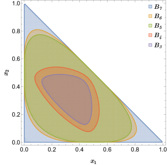
Figure 4: Detectable regions of $k$-reduction moment criteria with $k=2$. Each point represents a state with Schmidt number $3$ in the form of Eq. (55). The region of states whose Schmidt numbers can be detected by the $N$-th order moment-based criterion (that is, the set of states satisfying $B_{N}[\psi,2]\not\geq 0$) is illustrated in the plot. The higher the order is, the larger the detectable region becomes. When $N=7$, almost all states can be detected.

IV.4 The third order moment-based criterion

In this subsection, we provide more details on the third order moment-based $k$-reduction criterion, that is, $N=3$. Note that $q_{1}=kd_{B}-1>0$, so $B_{3}\geq 0$ iff $\det(B_{3}[\rho,k])\geq 0$. Accordingly, the criterion in Eq. (52) can be simplified as follows,

$$\text{ if }\mathrm{SN}(\rho)\leq k,\quad\text{then }\det(B_{3}[\rho,k])\geq 0.$$ (56)

Define

$$\begin{gathered}p_{n}\equiv\Tr(\rho^{n}),\quad a_{n}\equiv\Tr(\rho_{A}^{n}),\\ t_{2}\equiv\Tr_{A}[\rho_{A}\Tr_{B}(\rho^{2})].\end{gathered}$$ (57)

Then $\det(B_{3}[\rho,k])$ can be expressed as a polynomial of $k$ as follows,

$$\det(B_{3}[\rho,k])=\beta_{4}k^{4}+\beta_{3}k^{3}+\beta_{2}k^{2}+\beta_{1}k+\beta_{0},$$ (58)

where

$$\beta_{4} =d_{B}^{2}(a_{3}-a_{2}^{2}),$$ (59)

$$\beta_{3} =-4d_{B}(a_{3}-a_{2}^{2}),$$

$$\beta_{2} =d_{B}(3t_{2}-2a_{2}p_{2})-4a_{2}^{2}+3a_{3},$$

$$\beta_{1} =4a_{2}p_{2}-d_{B}p_{3}-3t_{2},$$

$$\beta_{0} =p_{3}-p_{2}^{2}.$$

Hence, to apply the criterion in Eq. (56), it remains to estimate the moments $p_{2},p_{3},a_{2},a_{3},t_{2}$.

IV.5 $k$-reduction moment criteria for pure states

Recall that the $k$-reduction criterion can certify the Schmidt number of any pure state. Here we clarify the performances of moment-based $k$-reduction criteria. The following theorem proved in Appendix C.1 shows that the $N$-th order moment-based $k$-reduction criterion can certify the Schmidt number of any pure state in $\mathcal{H}_{AB}$ when $N\geq 4d-1$, where $d=\min\{d_{A},d_{B}\}$. In addition, it is necessary to employ the $N$-th order moment-based $k$-reduction criterion with $N\geq 2d$ for certain pure states in $\mathcal{H}_{AB}$.

Theorem 5.

Suppose $|\psi\rangle\in\mathcal{H}_{AB}$ has Schmidt rank $r$ and $\tilde{r}$ distinct nonzero Schmidt coefficients denoted by $\{\ell_{j}\}_{j=0}^{\tilde{r}-1}$. If $N\geq 4\tilde{r}-1$, then the $N$-th order moment criterion can detect the state $|\psi\rangle$ as

$$B_{N}[\psi,k]\not\geq 0\quad\forall k=1,2,\ldots,r-1.$$ (60)

Let $L=(l_{n})_{n\in\mathbb{N}_{0}}$, $l_{n}=\sum_{j=0}^{\tilde{r}-1}\ell_{j}^{n}$, and

$$A_{0}\equiv\begin{cases}H(L_{1,N}),&N\textrm{ odd},\\ H[(r-1)L_{1,N-1}-L_{2,N}],&N\textrm{ even}.\end{cases}$$ (61)

If instead $N\leq 2\tilde{r}$ and

$$d_{B}>1+\frac{r\tilde{r}\mathcal{N}_{r-1}(\psi)}{\sigma_{\min}(A_{0})},$$ (62)

then the $N$-th order moment criterion cannot detect the state $|\psi\rangle$ as

$$B_{N}[\psi,r-1]\geq 0.$$ (63)

When $|\psi\rangle=|+_{r}\rangle$ is the maximally entangled state of Schmidt rank $r$, we have $\tilde{r}=1$, and Theorem 5 implies the following corollary. In this case, it suffices to apply the third order moment-based $k$-reduction criterion.

Corollary 2.

Given $|+_{r}\rangle$ defined in Eq. (4) and $1\leq k<r$, we have $B_{N}[+_{r},k]\not\geq 0$ for all $N\geq 3$.

IV.6 Certification of entanglement dimensionality of isotropic states

Given a Hilbert space $\mathcal{H}_{AB}$ with $d_{A}=d_{B}=d$, an isotropic state on $\mathcal{H}_{AB}$ is a state of the form

$$\rho_{F}\equiv\frac{1-F}{d^{2}-1}I+\frac{d^{2}F-1}{d^{2}-1}|+_{d}\rangle\langle+_{d}|,\quad F\in[0,1].$$ (64)

It has been proved that $\mathrm{SN}(\rho_{F})=\lceil dF\rceil$, and the $k$-reduction map can detect all isotropic states [14]. Here we show that the third order moment-based criterion is enough to certify all isotropic states as well. Meanwhile, the correlation matrix criterion and its moment-based variants in Eqs. (14) and (17) are equally effective. Propositions 4 and 5 below are proved in Appendices C and D, respectively.

Proposition 4.

Suppose $\rho_{F}$ is the isotropic state defined in Eq. (64) and $1\leq k\leq\lceil dF\rceil-1$. Then $B_{3}[\rho_{F},k]\not\geq 0$.

Proposition 5.

Suppose $\rho_{F}$ is the isotropic state defined in Eq. (64), and $T$ is its correlation matrix with respect to given local operator bases that satisfy the conditions in Eq. (7). Then all $d^{2}-1$ singular values of $T$ are equal to $(d^{2}F-1)/[d(d^{2}-1)]$ and

$$\|T\|_{1} =dF-d^{-1},\quad\|T\|_{2}^{2}=\frac{(d^{2}F-1)^{2}}{d^{2}(d^{2}-1)},$$ (65)

$$\|T\|_{4}^{4} =\frac{(d^{2}F-1)^{4}}{d^{4}(d^{2}-1)^{3}}.$$

In conjunction with the fact $\mathrm{SN}(\rho_{F})=\lceil dF\rceil$ and Eq. (10) we can conclude that the correlation matrix criterion can certify the Schmidt number of any isotropic state as well. Even if only the second and fourth moments are available, we can still deduce that $\|T\|_{1}\geq\|T\|_{2}^{3}/\|T\|_{4}^{2}=dF-d^{-1}$. Therefore, the moment-based criterion in Eq. (17) is equally effective, and so is the alternative in Eq. (14).

V Numerical results on detection ratios

To complement the theoretical analysis in Sec. IV, here we provide extensive numerical results on the detection ratios of the $N$-th order moment-based $k$-reduction criterion in Eq. (52) and moment-based CM criterion in Eq. (14). Given an ensemble $\mathcal{E}$ of quantum states, the detection ratio of the $N$-th order moment-based $k$-reduction criterion is defined as

$$\text{Pr}\left\{B_{N}[\rho,k]\not\geq 0\ :\ \rho\in\mathcal{E}\right\}.$$ (66)

Similarly, the detection ratio of the moment-based CM criterion is defined as

$$\text{Pr}\left\{(\|T\|_{2}^{2},\|T\|_{4}^{4})\not\in\mathcal{T}_{k}:\ \rho\in\mathcal{E}\right\}.$$ (67)

Not surprisingly, the detection ratios may strongly depend on the ensemble $\mathcal{E}$ under consideration. Nevertheless, for any given ensemble, a higher detection ratio is an indication of a higher performance. In the rest of this section we shall consider several concrete ensembles of quantum states, including the ensemble of pure states with a fixed Schmidt number, the ensemble of Haar random pure states with depolarizing noise, and the ensemble of mixed states with an induced measure.

V.1 Ensemble of pure states with a fixed Schmidt number

Define the ensemble

$$\mathcal{E}_{r}\equiv\left\{|\psi\rangle=\sum_{i=0}^{r-1}\sqrt{\lambda_{i}}|i\rangle_{A}\otimes|i\rangle_{B}\right\},$$ (68)

where $\{|i\rangle_{A}\},\{|i\rangle_{B}\}$ are elements of two orthonormal bases of $\mathcal{H}_{A}$ and $\mathcal{H}_{B}$, respectively, and $\{\lambda_{i}\}_{i=0}^{r-1}$ is uniformly distributed in the interior of a $(r-1)$-dimensional probability simplex [cf. Eq. (3)], which is also known as the Dirichlet distribution. By definition all states in $\mathcal{E}_{r}$ have Schmidt numbers equal to $r$. Here it is not necessary to consider local unitary transformations because the moment-based $k$-reduction criteria and correlation matrix criterion are both invariant under local unitary transformations. In numerical simulation we choose $d=d_{A}=d_{B}$.

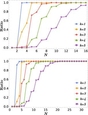
Figure 5: Detection ratio of the $N$-th order moment-based $k$-reduction criterion in Eq. (52) for the pure state ensemble $\mathcal{E}_{6}$ in Eq. (68) as a function of $N$. Here $d=8$ (upper plot) and $d=16$ (lower plot). The detection ratio increases monotonically with $N$, but decreases monotonically with $k$.

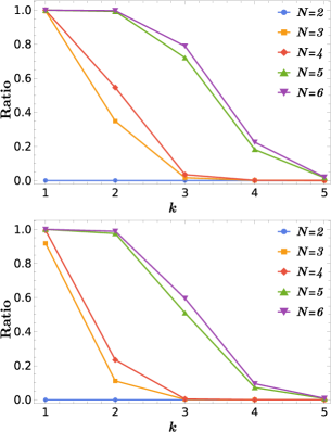
Figure 6: Detection ratio of the $N$-th order moment-based $k$-reduction criterion for the pure state ensemble $\mathcal{E}_{6}$ as a function of $k$. Here $d=8$ (upper plot) and $d=16$ (lower plot) as in Fig. 5.

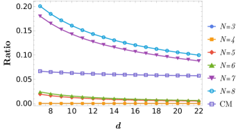
Figure 7: Detection ratios of the $N$-th order moment-based $k$-reduction criterion in Eq. (52) and moment-based CM criterion in Eq. (14) with $k=5$ for the ensemble $\mathcal{E}_{6}$ in Eq. (68) with $7\leq d\leq 22$. The $N$-th order moment-based $k$-reduction criterion has a larger detection ratio than the moment-based CM criterion when $N\geq 7$.

Figures 5 and 6 illustrate the detection ratio of the $N$-th order moment-based $k$-reduction criterion in Eq. (52) as a function of $N$ and $k$ for the ensemble $\mathcal{E}_{6}$ with two different local dimensions, namely, $d=8$ and $d=16$. As expected the detection ratio decreases monotonically with $k$, but increases monotonically with the order $N$ and eventually approaches 1 when $N$ is sufficiently large.

Now, we compare the detection ratios of the $N$-th order moment-based $k$-reduction criterion in Eq. (52) and moment-based correlation matrix criterion in Eq. (14). Figure 7 illustrates the results on the ensemble $\mathcal{E}_{6}$ as functions of the order $N$ and local dimension $d$, where $k=5$. According to this figure, the detection ratio of the moment-based correlation matrix criterion is almost independent of the local dimension, but the detection ratios of moment-based $k$-reduction criteria tend to decrease with the local dimension. Nevertheless, the $N$-th order moment-based $k$-reduction criterion has a larger detection ratio when $N$ is sufficiently large.

V.2 Ensemble of Haar random pure states with depolarizing noise

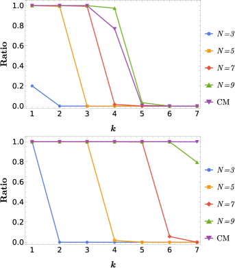
Figure 8: Detection ratios of different $k$-reduction moment criteria in Eq. (52) and moment-based CM criterion in Eq. (14) for the Haar random ensemble $\mathcal{E}_{\mathrm{Haar},0}$ in Eq. (39). Here $d=8$ (upper plot) and $d=16$ (lower plot) as in Fig. 5.

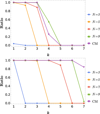
Figure 9: Detection ratios of different $k$-reduction moment criteria in Eq. (52) and moment-based CM criterion in Eq. (14) for the Haar random ensemble $\mathcal{E}_{\mathrm{Haar},0.1}$ in Eq. (39). Here $d=8$ (upper plot) and $d=16$ (lower plot) as in Fig. 5.

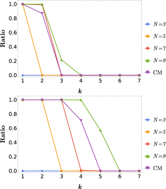
Figure 10: Detection ratios of different $k$-reduction moment criteria in Eq. (52) and moment-based CM criterion in Eq. (14) for the Haar random ensemble $\mathcal{E}_{\mathrm{Haar},0.5}$ in Eq. (39). Here $d=8$ (upper plot) and $d=16$ (lower plot) as in Fig. 5.

Next, we turn to the ensemble $\mathcal{E}_{\mathrm{Haar},\varepsilon}$ of Haar random states with depolarizing noise as defined in Eq. (39), where the parameter $\varepsilon$ characterizes the noise strength. Figures 8-10 illustrate the detection ratios of the $N$-th order moment-based $k$-reduction criterion in Eq. (52) and moment-based CM criterion in Eq. (14) for the ensemble $\mathcal{E}_{\mathrm{Haar},\varepsilon}$ with two different local dimensions and three different noise strengths. Not surprisingly, the detection ratios increase monotonically with $N$ but decrease monotonically with $k$ and $\varepsilon$. When $d=8$ and $N=9$ for example, the $N$-th order moment-based $k$-reduction criterion has a larger detection ratio than the moment-based CM criterion, but the situation is different when $d=16$.

V.3 Ensemble of mixed states with an induced measure

Table 4: Detection ratio of the $N$-th order moment-based $k$-reduction criterion in Eq. (52) with $N=16$ (corresponding to Algorithm 2 with $N^{*}=16$) for the ensemble $\mathcal{E}_{D,K}$ with $d_{A}=d_{B}=16$ and $D=d_{A}d_{B}=256$.

	2	3	4	5	6
3	1	1	1	1	1
4	1	1	1	1	0.8494
5	1	1	1	0.0014	0
6	1	1	0	0	0
7	1	0.0016	0	0	0
8	0.9390	0	0	0	0
9	0.0004	0	0	0	0

Table 5: Detection ratio of the moment-based CM criterion in Eq. (14) for the ensemble $\mathcal{E}_{D,K}$. Here $d_{A}=d_{B}=16$ and $D=d_{A}d_{B}=256$ as in Table 5.

	2	3	4	5	6
5	1	1	1	1	1
6	1	1	0.9322	0	0
7	1	0.0012	0	0	0
8	0.0042	0	0	0	0

Finally, we consider the ensemble $\mathcal{E}_{D,K}$ of mixed states with an induced measure, which is defined in Sec. III.5. In numerical simulation we choose $D=d^{2}=16^{2}$ and $K=2,3,4,5,6$. Tables 5 and 5 show the ratios of states with various lower bounds for the Schmidt numbers. The ratios in Table 5 are determined by moment-based $k$-reduction criteria described by Algorithm 2 with maximal order $N^{*}=16$ and $r=16$. The ratios in Table 5 are determined by moment-based CM criterion in Eq. (14). From the numerical results, we can see that the $k$-reduction moment criteria are weaker than moment-based CM criterion for $K=4,5,6$, but becomes stronger for $K=2$. When $K=3$, the performances are comparable.

VI Estimation of $k$-reduction moments

To certify the Schmidt number using moment-based $k$-reduction criteria, we need to estimate the $k$-reduction moments $q_{n}=\mathcal{R}_{k}(\rho)^{n}$ that appear in the entries of the Hankel matrices. Simple analysis shows that these moments can be expressed as follows,

$$\Tr\left[\text{poly}(\rho,\rho_{A}\otimes I_{B})\right].$$ (69)

In this section, we introduce two approaches for estimating these moments.

VI.1 Moment estimation by randomized measurements

Here we discuss moment estimation based on the classical shadow [12], which is a prototypical method based on randomized measurements. This method consists of two steps, namely, data acquisition and prediction. In the phase of data acquisition, we first randomly sample a unitary operator $U$ from a given unitary ensemble $\mathcal{U}$ on the Hilbert space $\mathcal{H}$ and apply it to the state $\rho$ under consideration. Then we perform a measurement in the computational basis and record the measurement outcome $b$. Based on $U$ and $b$, we can create a classical shadow of the unknown state as follows,

$$\hat{\rho}=\mathcal{M}^{-1}_{\mathrm{cs}}\left(U^{\dagger}|b\rangle\langle b|U\right).$$ (70)

Here $\mathcal{M}_{\mathrm{cs}}$ is the measurement channel, which depends on the ensemble $\mathcal{U}$, and $\mathcal{M}^{-1}_{\mathrm{cs}}$ is the inverse of $\mathcal{M}_{\mathrm{cs}}$ and is known as the reconstruction map. If $\mathcal{U}$ corresponds to the global Clifford group, then the above equation reduces to

$$\hat{\rho}=(D+1)U|b\rangle\langle b|U^{\dagger}-I,$$ (71)

where $D$ is the dimension of $\mathcal{H}$.

In the prediction phase, we need to estimate the expectation value of a given observable $O$ (generalization to more observables is straightforward). Given $M$ samples of the classical shadow we can construct an estimator based on the empirical mean as follows,

$$\hat{o}=\frac{1}{M}\sum_{m=0}^{M-1}\Tr(\hat{\rho}_{m}O).$$ (72)

The variance of this estimator is controlled by the shadow norm introduced in [12]. The worst-case variance is minimized when the ensemble $\mathcal{U}$ forms a unitary 3-design. Alternatively, we can employ the median-of-means to suppress the probability of large deviation.

In addition, the classical shadow method can be applied to estimating quadratic functions of $\rho$ that have the form $o=\Tr[O(\rho\otimes\rho)]$, where $O$ is now an operator on $\mathcal{H}^{\otimes 2}$. Here is a specific estimator [12],

$$\hat{o}=\frac{2}{M(M-1)}\sum_{m<n}^{M-1}\Tr[O(\hat{\rho}_{m}\otimes\hat{\rho}_{n})].$$ (73)

For example, the purity $\Tr(\rho^{2})$ can be estimated as follows,

$$\frac{2}{M(M-1)}\sum_{m<n}^{M-1}\Tr[\mathbb{W}_{(12)}(\hat{\rho}_{m}\otimes\hat{\rho}_{n})]$$

$$=\frac{2}{M(M-1)}\sum_{m<n}^{M-1}\Tr(\hat{\rho}_{m}\hat{\rho}_{n}),$$ (74)

where $\mathbb{W}_{(12)}$ is the swap operator on $\mathcal{H}^{\otimes 2}$. Other nonlinear functions can be estimated in a similar way.

Next, we turn to the estimation of reduction moments that are required for certifying the Schmidt number, assuming that $\mathcal{H}=\mathcal{H}_{AB}$ is a bipartite Hilbert space of dimension $D$. The following theorem clarifies the sample complexities of estimating the moments involved in the third order moment-based $k$-reduction criterion; see Appendix E for a proof.

Theorem 6.

Suppose $\rho\in\mathcal{S}(\mathcal{H}_{AB})$, $d_{A}=d_{B}=\sqrt{D}$, and we are given access to a unitary 3-design. Then the sample complexity of estimating the moments $p_{2},p_{3},a_{2},a_{3},t_{2}$ defined in Eq. (57) up to accuracy $\mathcal{O}(1)$ using the classical shadow method is $\mathcal{O}(D)$.

Note that the randomized measurements required to apply our certification protocol can be realized using a unitary 3-design, say the global Clifford group [27, 28], which is quite appealing to practical applications. By contrast, to apply the correlation matrix protocol [18, 19], it is necessary to use a unitary 4-design; moreover, a unitary 8-design is required to bound the variance.

VI.2 Moment estimation by permutation tests

Next, we show that the sample complexity of estimating the $k$-reduction moments can be reduced to $\mathcal{O}(1)$ if collective measurements based on permutation tests are accessible. Suppose $\mathcal{H}$ is a $D$-dimensional Hilbert space and $\rho_{1},\rho_{2},\ldots,\rho_{N}\in\mathcal{S}(\mathcal{H})$; then $\bigotimes_{n=1}^{N}\rho_{n}\in\mathcal{S}(\mathcal{H}^{\otimes N})$. Let $\mathbb{W}_{\pi}$ be the unitary operator tied to the standard cyclic permutation. Add an ancillary qubit prepared in the state $|+\rangle$ and apply the controlled unitary $|0\rangle\langle 0|\otimes I+|1\rangle\langle 1|\otimes\mathbb{W}_{\pi}$ on the entire system then yields

$$\frac{|0\rangle\langle 0|}{2}\otimes\bigotimes_{n=1}^{N}\rho_{n}+\frac{|1\rangle\langle 1|}{2}\otimes\mathbb{W}_{\pi}\bigotimes_{n=1}^{N}\rho_{n}\mathbb{W}^{-1}_{\pi},$$ (75)

$$+\frac{|0\rangle\langle 1|}{2}\otimes\bigotimes_{n=1}^{N}\rho_{n}\mathbb{W}^{-1}_{\pi}+\frac{|1\rangle\langle 0|}{2}\otimes\mathbb{W}_{\pi}\bigotimes_{n=1}^{N}\rho_{n}.$$

The reduced state on the ancilla qubit reads

$$\frac{I}{2}+\frac{1}{2}\Tr(\rho_{1}\rho_{2}\cdots\rho_{N})X.$$ (76)

Measure the ancilla qubit in the Pauli $X$ basis, then the probabilities of obtaining outcomes $\pm$ are given by

$$P_{\pm}=\frac{1}{2}\pm\frac{1}{2}\Tr(\rho_{1}\rho_{2}\cdots\rho_{N}),$$ (77)

which means

$$P_{+}-P_{-}=\Tr(\rho_{1}\rho_{2}\cdots\rho_{N}).$$ (78)

This result leads to a simple recipe for estimating the $N$-th moment $\Tr(\rho^{N})$ of a general quantum state $\rho\in\mathcal{S}(\mathcal{H})$, and the sample complexity is independent of the system size. This method can readily be applied to estimating all the relevant parameters featuring in the moment-based $k$-reduction criteria.

A relevant work about the quantum advantage enabled by permutation tests can be found in [44].

VII Conclusion

By virtue of the $k$-reduction map and moment method we proposed a family of criteria for certifying the entanglement dimensionality as quantified by the Schmidt number. These criteria do not require prior information about the target states, unlike fidelity-based methods. In addition, the $k$-reduction moments involved can be estimated by randomized measurements based on a unitary 3-design instead of a 4-design employed by the correlation matrix method. These features are quite appealing to practical applications. Furthermore, we showed that, if $k$-reduction moments with sufficiently high orders are accessible, then our criteria are equivalent to the $k$-reduction criterion and thus can certify the entanglement dimensionality of pure states accurately. Meanwhile, even the third $k$-reduction moment can certify the entanglement dimensionality of isotropic states. In the course of study, we clarified the basic properties of the spectrum of the $k$-reduced operator and showed that the $k$-reduction negativity is monotonic under LOCC for pure states.

Our work raises several questions that deserve further exploration. First, is the $k$-reduction negativity monotonic under LOCC for general mixed states? Second, how robust are the $k$-reduction moment criteria to statistical fluctuation. To clarify the second question would require knowledge about the perturbation theory of Hankel matrices, which we leave for future work. Third, can we construct better criteria for certifying the entanglement dimensionality by virtue of other $k$-positive maps in conjunction with the moment method? We hope that these questions can stimulate further progresses on the study of high-dimensional entanglement.

In this appendix we prove Theorems 1, 2, 4-6 and Propositions 3-5 presented in the main text.

Appendix A Proofs of Theorems 1, 2 and Proposition 3

A.1 Auxiliary lemmas

Here we introduce two auxiliary lemmas to clarify the basic properties of the matrix $\Omega_{k}(\boldsymbol{\lambda})$ defined in Eq. (25) and the function $\theta_{k}(\boldsymbol{\lambda})$ defined Eq. (26).

Lemma 2.

Suppose $k$ is a positive integer and $\boldsymbol{\lambda}\in\Delta_{d}$. Then $\Omega_{k}(\boldsymbol{\lambda})$ has at most one negative eigenvalue, and the function $\theta_{k}(\boldsymbol{\lambda})$ is Schur concave in $\boldsymbol{\lambda}$ and nonincreasing in $k$. Let $r$ be the number of positive entries in $\boldsymbol{\lambda}$; then

$$\rank(\Omega_{k}(\boldsymbol{\lambda}))=\begin{cases}r-1&k=r,\\ r&k\neq r.\end{cases}$$ (79)

If $k\geq r$, then $\Omega_{k}(\boldsymbol{\lambda})\geq 0$ and $\theta_{k}(\boldsymbol{\lambda})=0$. If $k<r$, then $-\theta_{k}(\boldsymbol{\lambda})$ is the unique negative eigenvalue of $\Omega_{k}(\boldsymbol{\lambda})$, and $\theta_{k}(\boldsymbol{\lambda})$ satisfies the following equation

$$\sum_{i=0}^{d-1}\frac{\lambda_{i}}{k\lambda_{i}+\theta_{k}(\boldsymbol{\lambda})}=1.$$ (80)

Proof.

Let $\tilde{\boldsymbol{\lambda}}$ be the vector obtained from $\boldsymbol{\lambda}$ by deleting the zero entries. Then $\Omega_{k}(\boldsymbol{\lambda})$ and $\Omega_{k}(\tilde{\boldsymbol{\lambda}})$ have the same nonzero eigenvalues, including the multiplicities, which means $\theta_{k}(\boldsymbol{\lambda})=\theta_{k}(\tilde{\boldsymbol{\lambda}})$. In addition, $\Omega_{k}(\boldsymbol{\lambda})$ and $\theta_{k}(\boldsymbol{\lambda})$ are continuous in $\boldsymbol{\lambda}$. Therefore, it suffices to prove Lemma 2 under the assumption $\boldsymbol{\lambda}>0$, which means $\lambda_{0},\lambda_{1},\ldots,\lambda_{d-1}>0$ and $r=d$.

Let $\Lambda=\operatorname{diag}(\lambda_{0},\lambda_{1},\ldots,\lambda_{d-1})$; then $\Omega_{k}(\boldsymbol{\lambda})=\Lambda^{1/2}\Omega^{\prime}\Lambda^{1/2}$, where $\Omega^{\prime}$ is the $d\times d$ matrix with entries $\Omega^{\prime}_{ij}=k\delta_{ij}-1$. Since $\Lambda$ is an invertible real diagonal matrix, $\Omega$ and $\Omega^{\prime}$ have the same rank and the same number of positive (negative) eigenvalues. It is straightforward to verify that $\Omega^{\prime}$ has $r-1$ eigenvalues equal to $k$ and one eigenvalue equal to $k-r$, which implies Eq. (79). If $k\geq r=d$, then $\Omega_{k}(\boldsymbol{\lambda})\geq 0$ and $\theta_{k}(\boldsymbol{\lambda})=0$. If $k<r$, then $\Omega_{k}(\boldsymbol{\lambda})$ has exactly one negative eigenvalue, which is equal to the smallest eigenvalue $-\theta_{k}$.

Suppose $k<r$ and $\boldsymbol{y}=(y_{0},y_{1},\dots,y_{d-1})^{\top}$ is an eigenvector of $\Omega_{k}(\boldsymbol{\lambda})$ associated with the eigenvalue $-\theta_{k}$. Then

$$k\lambda_{i}y_{i}-\sum_{j}\sqrt{\lambda_{i}\lambda_{j}}\,y_{j}=-\theta_{k}y_{i}\quad\forall i,$$ (81)

which implies that

$$y_{i}=\frac{\sqrt{\lambda_{i}}}{k\lambda_{i}+\theta_{k}}\left(\sum_{j=0}^{d-1}\sqrt{\lambda_{j}}\,y_{j}\right)\quad\forall i.$$ (82)

Note that $\sum_{j=0}^{d-1}\sqrt{\lambda_{j}}y_{j}\neq 0$, otherwise $\boldsymbol{y}$ is a zero vector. Now, we can deduce Eq. (80) by multiplying both sides with $\sqrt{\lambda_{i}}$ and summing over $i$.

Next, we prove that $\theta_{k}(\boldsymbol{\lambda})$ is nonincreasing in $k$ and Schur concave in $\boldsymbol{\lambda}$. If $k^{\prime}\geq k$, then $\Omega_{k^{\prime}}(\boldsymbol{\lambda})\geq\Omega_{k}(\boldsymbol{\lambda})$, which implies that $\theta_{k^{\prime}}(\boldsymbol{\lambda})\leq\theta_{k}(\boldsymbol{\lambda})$, so $\theta_{k}(\boldsymbol{\lambda})$ is nonincreasing in $k$.

If $k\geq d$, then $\theta_{k}(\boldsymbol{\lambda})=0$, so $\theta_{k}(\boldsymbol{\lambda})$ is Schur concave in $\boldsymbol{\lambda}$. To address the case with $k<d$, we need to introduce an auxiliary function,

$$G(y,k,\boldsymbol{\lambda})\equiv\sum_{i=0}^{d-1}\frac{\lambda_{i}}{k\lambda_{i}+y},\quad k,y>0,\quad\boldsymbol{\lambda}>0.$$ (83)

Then $\theta_{k}(\boldsymbol{\lambda})$ is the unique solution of $y>0$ to the equation $G(y,k,\boldsymbol{\lambda})=1$. Note that $G(y,k,\boldsymbol{\lambda})$ is nonincreasing in $y$, convex in each entry of $\boldsymbol{\lambda}$, and invariant under any permutation of these entries. Therefore, $G(y,k,\boldsymbol{\lambda})$ is Schur concave in $\boldsymbol{\lambda}$. Suppose $\boldsymbol{\lambda}^{\prime}\in\Delta_{d}$ and $\boldsymbol{\lambda}^{\prime}\prec\boldsymbol{\lambda}$; let $y=\theta_{k}(\boldsymbol{\lambda})$, then $G(y,k,\boldsymbol{\lambda}^{\prime})\geq G(y,k,\boldsymbol{\lambda})=1$, which implies that $\theta_{k}(\boldsymbol{\lambda}^{\prime})\geq y=\theta_{k}(\boldsymbol{\lambda})$. Therefore, $\theta_{k}(\boldsymbol{\lambda})$ is Schur concave in $\boldsymbol{\lambda}$, which completes the proof of Lemma 2. ∎

Lemma 3.

Suppose $k$ is a positive integer, $\boldsymbol{\lambda}\in\Delta_{d}$ has $r$ nonzero entries with $\tilde{r}$ distinct nonzero values labeled as $\{\ell_{j}\}_{j=0}^{\tilde{r}-1}$, where $\ell_{j}$ has multiplicity $m_{j}$. Let $\widetilde{\Omega}_{k}(\boldsymbol{\lambda})$ be the $\tilde{r}\times\tilde{r}$ matrix with entries $\widetilde{\Omega}_{k}(\boldsymbol{\lambda})_{ij}=k\ell_{i}\delta_{ij}-\sqrt{m_{i}m_{j}\ell_{i}\ell_{j}}$. Then the eigenvalues $\{\omega_{j}\}_{j=0}^{\tilde{r}-1}$ of $\widetilde{\Omega}_{k}(\boldsymbol{\lambda})$ are nondegenerate and satisfy

$$-1<\omega_{\tilde{r}-1}<k\ell_{\tilde{r}-1}<\omega_{\tilde{r}-2}<k\ell_{\tilde{r}-2}<\cdots<\omega_{0}<k\ell_{0}.$$ (84)

In addition,

$$\rank(\widetilde{\Omega}_{k}(\boldsymbol{\lambda})) =\begin{cases}\tilde{r}-1&k=r,\\ \tilde{r}&k\neq r,\end{cases}$$ (85)

$$\sigma(\Omega_{k}(\boldsymbol{\lambda})) =\bigcup_{j=0}^{\tilde{r}-1}\{k\ell_{j}\}^{\times(m_{j}-1)}\cup\sigma\bigl{(}\widetilde{\Omega}_{k}(\boldsymbol{\lambda})\bigr{)}\cup\{0\}^{\times\left(d-r\right)}.$$ (86)

Proof of Lemma 3.

According to Cauchy Interlacing theorem, the eigenvalues $\{\omega_{j}\}_{j=0}^{\tilde{r}-1}$ of $\widetilde{\Omega}_{k}(\boldsymbol{\lambda})$ satisfy

$$-1<\omega_{\tilde{r}-1}\leq k\ell_{\tilde{r}-1}\leq\omega_{\tilde{r}-2}\leq k\ell_{\tilde{r}-2}\leq\cdots\leq\omega_{0}\leq k\ell_{0}.$$ (87)

Here the first inequality holds because $\ell_{j}>0$ and $\sum_{j=0}^{\tilde{r}-1}m_{j}\ell_{j}=1$. In addition, using proof by contradiction, it is straightforward to verify that $k\ell_{j}$ is not an eigenvalue of $\widetilde{\Omega}_{k}(\boldsymbol{\lambda})$ for $j=0,1,\ldots,\tilde{r}-1$. So all the inequalities in the above equation are necessarily strict, which confirms Eq. (84) and shows that the eigenvalues $\{\omega_{j}\}_{j=0}^{\tilde{r}-1}$ of $\widetilde{\Omega}_{k}(\boldsymbol{\lambda})$ are nondegenerate.

Next, we prove Eq. (86) before Eq. (85). To this end, we need to introduce the following index sets,

$$\mathcal{I}_{j}\equiv\{i:\lambda_{i}=\ell_{j}\},\quad j=0,1,\ldots,\tilde{r}-1;\quad\mathcal{I}_{\tilde{r}}\equiv\{i:\lambda_{i}=0\}.$$ (88)

On this basis we can define the following subspaces of $\mathbb{R}^{d}$,

$$V_{j}=\biggl{\{}v\in\mathbb{R}^{d}:v_{i}=0\;\forall i\notin\mathcal{I}_{j},\;\sum_{i}v_{i}=0\biggr{\}},\quad j=0,1,\ldots,\tilde{r}-1;\quad V_{\tilde{r}}=\bigl{\{}v\in\mathbb{R}^{d}:v_{i}=0\;\forall i\notin\mathcal{I}_{\tilde{r}}\bigr{\}}.$$ (89)

Then every nonzero vector in $V_{j}$ is an eigenvector of $\Omega_{k}(\boldsymbol{\lambda})$ with eigenvalue $k\ell_{j}$, where $\ell_{\tilde{r}}=0$. In addition,

$$\dim V_{j}=|\mathcal{I}_{j}|=m_{j}-1,\quad j=0,1,\ldots,\tilde{r}-1;\quad\dim V_{\tilde{r}}=|\mathcal{I}_{\tilde{r}}|=d-r,$$ (90)

$$V_{j_{1}}\perp V_{j_{2}},\quad 0\leq j_{1}<j_{2}\leq\tilde{r}.$$ (91)

Define $W\equiv(V_{1}+V_{2}+\cdots+V_{\tilde{r}})^{\perp}$. Then $W$ is an invariant subspace of $\Omega_{k}(\boldsymbol{\lambda})$ that has dimension $\tilde{r}$ and is spanned by the following $\tilde{r}$ vectors in $\mathbb{R}^{d}$,

$$(v_{j})_{i}=\begin{cases}\frac{1}{\sqrt{m_{j}}}&i\in\mathcal{I}_{j}\\ 0&i\not\in\mathcal{I}_{j}\end{cases}\quad j=0,1,\ldots,\tilde{r}-1.$$ (92)

Now, consider the following map from $\mathbb{R}^{\tilde{r}}$ to $\mathbb{R}^{d}$,

$$x\mapsto v_{x}\equiv\sum_{j=0}^{\tilde{r}}x_{j}v_{j}.$$ (93)

Then $v_{x}$ is an eigenvector of $\Omega_{k}(\boldsymbol{\lambda})$ iff $x$ is an eigenvector of $\widetilde{\Omega}_{k}(\boldsymbol{\lambda})$ with the same eigenvalue. This observation implies Eq. (86).

Equation (85) is a simple corollary of Eqs. (79) and (86) given that $\sum_{j=0}^{\tilde{r}-1}(m_{j}-1)=r-\tilde{r}$, which completes the proof of Lemma 3. ∎

A.2 Proof of Theorem 1

Proof.

Without loss of generality we can assume that $|\psi\rangle$ has the following Schmidt decomposition: $|\psi\rangle=\sum_{i=0}^{d-1}\sqrt{\lambda_{i}}|ii\rangle$, where $d=\min\{d_{A},d_{B}\}=d_{A}$. Define $\mathcal{W}_{1}\equiv\mathrm{span}\left(\{|ii\rangle\}_{i=0}^{d-1}\right)$ and $\mathcal{W}_{2}=\mathcal{W}_{1}^{\perp}$. Then $\mathcal{W}_{1}$ and $\mathcal{W}_{2}$ have dimensions $d$ and $d(d_{B}-1)$, respectively. The $k$-reduced operator $\mathcal{R}_{k}(\rho)$ can be expressed as follows,

$$\mathcal{R}_{k}(\rho)=k\sum_{i=0}^{d-1}\lambda_{i}\ket{i}\bra{i}\otimes I_{B}-\sum_{i,j=0}^{d-1}\sqrt{\lambda_{i}\lambda_{j}}\ket{ii}\bra{jj}=R_{1}+R_{2},$$ (94)

where

$$R_{1}\equiv k\sum_{i=0}^{d-1}\lambda_{i}\ket{ii}\bra{ii}-\sum_{i,j=0}^{d-1}\sqrt{\lambda_{i}\lambda_{j}}\ket{ii}\bra{jj},\quad R_{2}\equiv k\sum_{i=0}^{d-1}\sum_{j=0,j\neq i}^{d_{B}-1}\lambda_{i}\ket{ij}\bra{ij}$$ (95)

are supported in $\mathcal{W}_{1},\mathcal{W}_{2}$, respectively. Note $\sigma(R_{1})=\sigma(\Omega_{k}(\boldsymbol{\lambda}))$ and $\sigma(R_{2})=[k\sigma(\psi)]^{\times(d_{B}-1)}$. Therefore,

$$\sigma(\mathcal{R}_{k}(\rho))=\sigma(R_{1})\cup\sigma(R_{2})=\sigma(\Omega_{k}(\boldsymbol{\lambda}))\cup\{k\sigma(\psi)\}^{\times(d_{B}-1)},$$ (96)

which confirms Eq. (27). Since all eigenvalues of $R_{2}$ are non-negative, it follows that $\mathcal{R}_{k}(\rho)$ and $\Omega_{k}(\boldsymbol{\lambda})$ have the same negative spectrum, including multiplicities. According to Lemma 2, if $k\geq r$, then $\Omega_{k}(\boldsymbol{\lambda})\geq 0$ and $\mathcal{R}_{k}(\rho)\geq 0$. If instead $1\leq k<r$, then both $\Omega_{k}(\boldsymbol{\lambda})$ and $\mathcal{R}_{k}(\rho)$ have exactly one negative eigenvalue.

Let $\{\ell_{j}\}_{j=0}^{\tilde{r}-1}$ be the set of distinct nonzero Schmidt coefficients of $|\psi\rangle$, where $\ell_{j}$ has multiplicity $m_{j}$. In conjunction with Lemma 3 we can further deduce that

$$\sigma(\mathcal{R}_{k}(\rho))=\bigcup_{j=0}^{\tilde{r}-1}\{k\ell_{j}\}^{\times(d_{B}m_{j}-1)}\cup\sigma\bigl{(}\widetilde{\Omega}_{k}(\boldsymbol{\lambda})\bigr{)}\cup\{0\}^{\times d_{B}(d-r)},$$ (97)

where $\widetilde{\Omega}_{k}(\boldsymbol{\lambda})$ is the $\tilde{r}\times\tilde{r}$ matrix defined in Lemma 3, and its eigenvalues satisfy Eq. (84). Moreover, $\widetilde{\Omega}_{k}(\boldsymbol{\lambda})$ is nonsingular when $k\neq r$ and has exactly one eigenvalue equal to 0 when $k=r$. Therefore, $\mathcal{R}_{k}(\rho)$ has $2\tilde{r}$ distinct nonzero eigenvalues when $k\neq r$ and $2\tilde{r}-1$ distinct nonzero eigenvalues when $k=r$. In any case, $\mathcal{R}_{k}(\rho)$ has at most $2\tilde{r}$ distinct nonzero eigenvalues. This observation completes the proof of Theorem 1. ∎

A.3 Proof of Theorem 2

Proof.

According to Theorem 1 and Lemma 2, $\mathcal{N}_{k}(\psi)=\theta_{k}(\boldsymbol{\lambda})$ is Schur concave in $\boldsymbol{\lambda}$ and nonincreasing in $k$. Next, suppose $\mathrm{SN}(\psi)=r$ and let $\boldsymbol{\lambda}^{\prime}\equiv\left(r^{-1},\ldots,r^{-1},0,\ldots,0\right)\in\Delta_{d}$, where the value $r^{-1}$ is repeated $r$ times. Then $\boldsymbol{\lambda}\succ\boldsymbol{\lambda}^{\prime}$, which implies that $\mathcal{N}_{k}(\boldsymbol{\lambda})=\theta_{k}(\boldsymbol{\lambda})\leq\theta_{k}(\boldsymbol{\lambda}^{\prime})=1-k/r$. ∎

A.4 Proof of Proposition 3

Proof.

Define $\mathcal{W}_{0}\equiv\mathrm{span}\left(\{|i_{A}\rangle\otimes|j_{B}\rangle\}_{i,j=0}^{r-1}\right)$. Let $I_{0}$ be the projector onto this subspace and $I_{1}=I-I_{0}$, then

$$\rho_{\varepsilon,r}=\left[(1-\varepsilon)|+_{r}\rangle\langle+_{r}|+\varepsilon\frac{I_{0}}{d_{A}d_{B}}\right]+\varepsilon\frac{I_{1}}{d_{A}d_{B}}=(1-\varepsilon^{\prime})\rho^{\mathrm{ef}}_{\varepsilon,r}+\varepsilon^{\prime}\frac{I_{1}}{d_{A}d_{B}-r^{2}},$$ (98)

where

$$\rho^{\mathrm{ef}}_{\varepsilon,r}\equiv\frac{1-\varepsilon}{1-\varepsilon^{\prime}}|+_{r}\rangle\langle+_{r}|+\frac{\varepsilon}{1-\varepsilon^{\prime}}\frac{I_{0}}{d_{A}d_{B}},\quad\varepsilon^{\prime}\equiv\varepsilon\frac{d_{A}d_{B}-r^{2}}{d_{A}d_{B}}.$$ (99)

Every pure state decomposition of $\rho^{\mathrm{ef}}_{\varepsilon,r}$ corresponds to a pure state decomposition of $\rho_{\varepsilon,r}$ with the same maximal Schmidt number. Thus, $\mathrm{SN}(\rho_{\varepsilon,r})\leq\mathrm{SN}\left(\rho^{\mathrm{ef}}_{\varepsilon,r}\right)$. Note that $\rho^{\mathrm{ef}}_{\varepsilon,r}$ is an isotropic state of a bipartite system with local dimensions both equal to $r$. It is known that the Schmidt number of

$$\frac{r^{2}F-1}{r^{2}-1}|+_{r}\rangle\langle+_{r}|+\frac{1-F}{r^{2}-1}I_{0}$$ (100)

equals $\lceil rF\rceil$ [14]. Now, suppose $F$ is determined by the equation

$$\frac{r^{2}F-1}{r^{2}-1}=\frac{1-\varepsilon}{1-\varepsilon^{\prime}}.$$ (101)

Then

$$\mathrm{SN}(\rho_{\varepsilon,r})\leq\mathrm{SN}\left(\rho^{\mathrm{ef}}_{\varepsilon,r}\right)=\lceil rF\rceil=\left\lceil\frac{r^{2}-1}{r}\cdot\frac{d_{A}d_{B}(1-\varepsilon)}{d_{A}d_{B}(1-\varepsilon)+\varepsilon r^{2}}+\frac{1}{r}\right\rceil=\left\lceil\frac{(1+u)r}{1+r^{2}u}\right\rceil,$$ (102)

which confirms the upper bound in Eq. (37).

On the other hand, if

$$k\leq\left\lceil\frac{(1+u)r}{1+d_{B}ru}\right\rceil-1,$$ (103)

then $\mathcal{N}_{k}(\rho_{\varepsilon,r})>0$ by Proposition 2, which implies that

$$\mathrm{SN}(\rho_{\varepsilon,r})\geq\frac{(1+u)r}{1+d_{B}ru}$$ (104)

and confirms the lower bound in Eq. (37).

Finally, if $r\leq\sqrt{d_{A}}$ and $\varepsilon<1/2$, then we have $u<(d_{A}d_{B})^{-1}$ and

$$\frac{(1+u)r}{1+d_{B}ru}>r-1,$$ (105)

which implies that $\mathrm{SN}(\rho_{\varepsilon,r})=r$. This observation completes the proof of Proposition 3. ∎

Appendix B Proofs of Theorems 3 and 4

B.1 An auxiliary lemma

Given $x\in\mathbb{R}$ and $l\in\mathbb{N}_{0}$, define

$$e(x,l)\equiv\left(1,x,x^{2},\ldots,x^{l}\right)^{\top}.$$ (106)

Consider the moment sequence $S=(s_{n})_{n\in\mathbb{N}_{0}}$ with $s_{n}=x^{n}$ and let $S_{k,2l+k}\equiv(s_{k},s_{k+1},\ldots,s_{2l+k})$ be a truncated subsequence. The Hankel matrix $H(S_{k,2l+k})$ has entries

$$[H(S_{k,2l+k})]_{m,n}=s_{m+n+k}=x^{k}e(x,l)_{m}e(x,l)_{n}\quad m,n=0,1,\ldots,l.$$ (107)

So the Hankel matrix itself can be expressed as follows,

$$H(S_{k,2l+k})=x^{k}e(x,l)e(x,l)^{\top}.$$ (108)

Next, as a generalization, consider the moment sequence $S^{\prime}=(s^{\prime}_{n})_{n\in\mathbb{N}_{0}}$ with $s^{\prime}_{n}=\sum_{i=0}^{\chi-1}m_{i}x_{i}^{n}$, where $x_{i}\in\mathbb{R}$ and $m_{i}\in\mathbb{N}$. By linearity, we have

$$H(S^{\prime}_{k,2l+k})=\sum_{i=0}^{\chi-1}m_{i}x_{i}^{k}e(x_{i},l)e(x_{i},l)^{\top}.$$ (109)

The following lemma is instructive to understanding the properties of the Hankel matrix $H(S^{\prime}_{k,2l+k})$.

Lemma 4.

Suppose $\{x_{i}\}_{i=0}^{\chi-1}$ is a set of distinct real numbers and $l\in\mathbb{N}_{0}$. Then

$$\rank\left(\left[e(x_{0},l),e(x_{1},l),\ldots,e(x_{\chi-1},l)\right]\right)=\min\left\{l+1,\chi\right\}.$$ (110)

If $l+1\geq\chi$, then the set $\{e(x_{i},l)\}_{i=0}^{\chi-1}$ is linearly independent.

Proof.

Let $V$ be the Vandermonde matrix associated with the set $\{x_{i}\}_{i=0}^{\chi-1}$, that is,

$$V_{ij}\equiv x_{i}^{j}\quad i,j=0,1,\ldots,\min\left\{l,\chi-1\right\}.$$ (111)

Thanks to the Vandermonde determinant formula, we have

$$\det(V)=\prod_{0\leq i<j\leq\dim(V)-1}(x_{i}-x_{j})\neq 0.$$ (112)

Therefore,

$$\min\{l+1,\chi\}=\mathrm{rank}(V)\leq\rank\left(\left[e(x_{0},l),e(x_{1},l),\ldots,e(x_{\chi-1},l)\right]\right)\leq\min\left\{l+1,\chi\right\},$$ (113)

which implies Eq. (110).

If $l+1\geq\chi$, then $\rank\left(\left[e(x_{0},l)\cdots e(x_{\chi-1},l)\right]\right)=\chi$ by Eq. (110), so the set $\{e(x_{i},l)\}_{i=0}^{\chi-1}$ is linearly independent, which completes the proof of Lemma 4. ∎

B.2 Proofs of Theorems 3 and 4

In preparation for proving Theorems 3 and 4, suppose $\rho\in\mathcal{S}(\mathcal{H}_{AB})$ and $\mathcal{R}_{k}(\rho)$ has $\chi$ distinct nonzero eigenvalues, namely, $\{x_{i}\}_{i=0}^{\chi-1}$, where $x_{i}$ has multiplicity $m_{i}$. According to the definition in Eq. (51) and the formula in Eq. (109), $B_{N}[\rho,k]$ can be expressed as follows,

$$B_{N}[\rho,k] =\sum_{i=0}^{\chi-1}m_{i}p_{N,k}(x_{i})b_{N}(x_{i})b_{N}(x_{i})^{\top},$$ (114)

where

$$b_{N}(x) \equiv e(x,\lfloor(N-1)/2\rfloor)=\left(1,x,x^{2},\ldots,x^{\lfloor\frac{N-1}{2}\rfloor}\right)^{\top},$$ (115)

$$p_{N,k}(x) \equiv\begin{cases}x,&N\textrm{ odd};\\ x(k-x),&N\textrm{ even}.\end{cases}$$ (116)

Proof of Theorem 3.

Suppose $\mathcal{R}_{k}(\rho)$ has $\chi$ different nonzero eigenvalues $\{x_{i}\}_{i=0}^{\chi-1}$, where $x_{i}$ has multiplicity $m_{i}\geq 1$. Then $B_{N}$ has the decomposition in Eq. (114) with $x_{i}\in\mathbb{R}$ and $m_{i}\in\mathbb{N}$. Since $\mathrm{SN}(\rho)\leq k$ by assumption, we have $0\leq x_{i}\leq k$ for all $i$ thanks to Theorem 1 and Corollary 1. Therefore, $m_{i}p_{N,k}(x_{i})\geq 0$ for all $i$, which means $B_{N}\geq 0$ and completes the proof of Theorem 3. ∎

Proof of Theorem 4.

Let $\{x_{i}\}_{i=0}^{\chi-1}$ be the set of distinct nonzero eigenvalues of $\mathcal{R}_{k}(\rho)$ and denote by $m_{i}$ the multiplicity of $x_{i}$. Then $B_{N}$ has the decomposition in Eq. (114) with $m_{i}\in\mathbb{N}$ and $x_{i}\in[-1+k/d,k]$ by Corollary 1. In addition, $\{b_{N}(x_{i})\}_{i=0}^{\chi-1}$ are linearly independent according to Lemma 4, given that $N\geq 2\chi-1$ by assumption. Hence, $B_{N}\geq 0$ iff $m_{i}p_{N,k}(x_{i})\geq 0$ for all $i$. Meanwhile, $m_{i}p_{N,k}(x_{i})\geq 0$ iff $x_{i}\geq 0$. Therefore, $B_{N}\geq 0$ iff $x_{i}\geq 0$ for all $i$, that is, $\mathcal{R}_{k}(\rho)\geq 0$, which completes the proof of Theorem 4. ∎

Appendix C Proofs of Theorem 5 and Proposition 4

C.1 Proof of Theorem 5

Proof of Theorem 5.

Let $k=1,2,\ldots,r-1$; then $\mathcal{R}_{k}(\psi)\not\geq 0$ and $\mathcal{R}_{k}(\psi)$ has at most $2\tilde{r}$ distinct nonzero eigenvalues according to Theorem 1. Suppose $N\geq 4\tilde{r}-1$; then $\mathcal{R}_{k}(\psi)\not\geq 0$ iff $B_{N}[\psi,k]\not\geq 0$ thanks to Theorem 4. Therefore, $B_{N}[\psi,k]\not\geq 0$, which confirms Eq. (60).

Let $\{\ell_{j}\}_{j=0}^{\tilde{r}-1}$ be the set of distinct nonzero Schmidt coefficients of $|\psi\rangle$, where $\ell_{j}$ has multiplicity $m_{j}$. According to Lemma 3, the spectrum of $\mathcal{R}_{k}(\psi)$ can be expressed as follows

$$\sigma(\mathcal{R}_{k}(\psi))=\bigcup_{j=0}^{\tilde{r}-1}\{k\ell_{j}\}^{\times(d_{B}m_{j}-1)}\cup\{\omega_{j}\}_{j=0}^{\tilde{r}-1}\cup\{0\}^{\times d_{B}(d-r)},$$ (117)

where $\omega_{j}$ for $j=0,1,\ldots,\tilde{r}-1$ are the eigenvalues of the matrix $\widetilde{\Omega}(\boldsymbol{\lambda})$ defined in Lemma 3. Note that $\sum_{j}m_{j}=r$ and

$$0<k\ell_{j}\leq k,\quad-1<\omega_{j}<k\quad\forall j=0,1,\ldots,\tilde{r}-1;\quad 0<\omega_{j}<k\quad\forall j=0,1,\ldots,\tilde{r}-2.$$ (118)

In conjunction with Eqs. (51) and (114), the Hankel matrix $B_{N}[\psi,k]$ can be expressed as follows,

$$\begin{gathered}B_{N}=B_{N}[\psi,k]=A_{1}+A_{2},\\ A_{1}\equiv\sum_{j=0}^{\tilde{r}-1}p_{N,k}(\omega_{j})b_{N}(\omega_{j})b_{N}(\omega_{j})^{\top},\quad A_{2}\equiv\sum_{j=0}^{\tilde{r}-1}(d_{B}m_{j}-1)p_{N,k}(k\ell_{j})b_{N}(k\ell_{j})b_{N}(k\ell_{j})^{\top},\end{gathered}$$ (119)

where $b_{N}$ and $p_{N,k}(x)$ are defined in Eqs. (115) and (116), respectively. Note that $p_{N,k}(k\ell_{j})\geq 0$, while $p_{N,k}(\omega_{j})$ has the same sign as $\omega_{j}$ for $j=0,1,\ldots,\tilde{r}-1$.

Now suppose $N\leq 2\tilde{r}$ and $k=r-1$. Let $\ell_{\min}\equiv\min_{j}\{\ell_{j}\}$ and $\omega_{\min}\equiv\min_{j}\{\omega_{j}\}=-\mathcal{N}_{r-1}(\psi)$; then $\omega_{\min}\in(-1,0)$. In addition, $A_{1}$, $A_{2}$, and $B_{N}$ are square matrices with at most $\tilde{r}$ rows (columns), and $1\leq\|b_{N}(\omega_{\min})\|_{2}^{2}\leq\tilde{r}$. In conjunction with Lemma 4, we can deduce that $A_{2}$ has full rank, which means $\imaginary(A_{1})\subset\imaginary(A_{2})$.

By definition in Eq. (61) we have

$$A_{0}=\sum_{j=0}^{\tilde{r}-1}p_{N,r-1}[(r-1)\ell_{j}]b_{N}[(r-1)\ell_{j}]b_{N}[(r-1)\ell_{j}]^{\top},$$ (120)

which means $\sigma_{\min}(A_{2})\geq(d_{B}-1)\sigma_{\min}(A_{0})$ given that $m_{j}\geq 1$ and $p_{N,r-1}[(r-1)\ell_{j}]\geq 0$ for all $j$. If in addition $N$ is odd, then

$$\sigma_{\min}(A_{1}) \geq p_{N,r-1}(\omega_{\min})\|b_{N}(\omega_{\min})\|_{2}^{2}\geq\tilde{r}\omega_{\min},$$ (121)

$$\sigma_{\min}\left(B_{N}\right) \geq\sigma_{\min}(A_{1})+\sigma_{\min}(A_{2})\geq\tilde{r}\omega_{\min}+(d_{B}-1)\sigma_{\min}(A_{0}).$$ (122)

If instead $N$ is even, then

$$\sigma_{\min}(A_{1}) \geq p_{N,r-1}(\omega_{\min})\|b_{N}(\omega_{\min})\|_{2}^{2}\geq r\tilde{r}\omega_{\min},$$ (123)

$$\sigma_{\min}(B_{N}) \geq r\tilde{r}\omega_{\min}+(d_{B}-1)\sigma_{\min}(A_{0}).$$ (124)

Note that $\omega_{\min}=-\mathcal{N}_{r-1}(\psi)$ and that Eq. (124) holds in both cases. If the condition in Eq. (62) is satisfied, that is, $d_{B}-1\geq r\tilde{r}\mathcal{N}_{r-1}(\psi)/\sigma_{\min}(A_{0})$, then $\sigma_{\min}(B_{N})>0$, which confirms Eq. (63) and completes the proof of Theorem 5. ∎

C.2 Proof of Proposition 4

Proof.

The $k$-reduced operator $\mathcal{R}_{k}(\rho_{F})$ has spectrum

$$\sigma(\mathcal{R}_{k}(\rho_{F}))=\left\{\lambda_{1}\right\}^{\times(d^{2}-1)}\sqcup\left\{\lambda_{0}\right\},\quad\lambda_{1}=\frac{F-1}{d^{2}-1}+\frac{k}{d}>0,\quad\lambda_{0}=\frac{k}{d}-F.$$ (125)

Note that $\mathcal{R}_{k}(\rho_{F})$ has at most two distinct nonzero eigenvalues. Given $N=3$, then $B_{N}[\rho_{F},k]\geq 0$ iff $\mathcal{R}_{k}(\rho_{F})\geq 0$ according to Theorem 4. If in addition $k\leq\lceil dF\rceil-1$, then $\lambda_{0}<0$ and $\mathcal{R}_{k}(+_{r})\not\geq 0$, which further implies that $B_{N}[+_{r},k]\not\geq 0$. ∎

Appendix D Proof of Proposition 5

Proof.

By assumption the local Hilbert spaces $\mathcal{H}_{A}$ and $\mathcal{H}_{B}$ have the same dimension $d$ and thus can be identified as two copies of a $d$-dimensional Hilbert space $\mathcal{H}$. Let $\{P_{j}\}_{j=1}^{d^{2}-1}$ be an orthogonal basis on $\mathcal{L}_{0}^{\mathrm{H}}(\mathcal{H})$ that satisfies the normalization condition $\tr(P_{j}P_{k})=d\delta_{j,k}$. Then $\{P_{j}^{*}\}_{j=1}^{d^{2}-1}$ is also an orthogonal basis on this space. In conjunction with the definition of $\rho_{F}$ in Eq. (64), the entries of its correlation matrix $T$ can be calculated as follows,

$$T_{jk} =\frac{d^{2}F-1}{d(d^{2}-1)}\langle+_{d}|P_{j}\otimes P^{*}_{k}|+_{d}\rangle=\frac{d^{2}F-1}{d^{2}(d^{2}-1)}\sum_{m,n=0}^{d-1}\langle mm|P_{j}\otimes P_{k}^{*}|nn\rangle$$

$$=\frac{d^{2}F-1}{d^{2}(d^{2}-1)}\sum_{m,n=0}^{d-1}\langle m|P_{j}|n\rangle\langle n|P_{k}^{\dagger}|m\rangle=\frac{d^{2}F-1}{d^{2}(d^{2}-1)}\Tr\bigl(P_{j}P_{k}^{\dagger}\bigr{missing})=\frac{d^{2}F-1}{d(d^{2}-1)}\delta_{j,k},$$ (126)

where $j,k=1,2,\ldots,d^{2}-1$. Therefore, all singular values of $T$ are equal to $\frac{d^{2}F-1}{d(d^{2}-1)}$, which has multiplicity $d^{2}-1$. As a simple corollary, we have

$$\|T\|_{1} =(d^{2}-1)\times\frac{d^{2}F-1}{d(d^{2}-1)}=\frac{d^{2}F-1}{d},$$ (127)

$$\|T\|_{2}^{2} =(d^{2}-1)\times\left[\frac{d^{2}F-1}{d(d^{2}-1)}\right]^{2}=\frac{(d^{2}F-1)^{2}}{d^{2}(d^{2}-1)},$$

$$\|T\|_{4}^{4} =(d^{2}-1)\times\left[\frac{d^{2}F-1}{d(d^{2}-1)}\right]^{4}=\frac{(d^{2}F-1)^{4}}{d^{4}(d^{2}-1)^{3}},$$

which completes the proof of Proposition 5. ∎

Appendix E Proof of Theorem 6

In this appendix, we will show that given access to a unitary 3-design, the sample complexity of estimating $\Tr(\rho^{2}),\Tr(\rho^{3})$ and $\Tr_{A}[\rho_{A}\Tr_{B}(\rho^{2})]$ using the classical shadow methods are $\mathcal{O}(D)$, where $D$ is the dimension of $\rho$. Note that the protocol for estimating $a_{2},a_{3}$ is identical to that of $p_{2},p_{3}$, but in a Hilbert space with dimension $\sqrt{D}$ instead. Hence, the sample complexity of estimating $a_{2},a_{3}$ is strictly smaller than that of $p_{2},p_{3}$, and the sample complexity of the third order moment-based $k$-reduction criterion is $\mathcal{O}(D)$.

E.1 An auxiliary lemma

In order to compute the variance for the estimators of $p_{2},p_{3}$ and $t_{2}$, we need to estimate the average over $k$-fold random unitaries. Given a Hilbert space $\mathcal{H}$ with dimension $D$. Let $\mu(U)$ denote Haar random distribution of unitaries on $\mathcal{H}$. It has been proved that (Proposition 2.3 in [45])

$$\Phi^{(k)}(A)\equiv\int d\mu(U)U^{\otimes k}A(U^{\dagger})^{\otimes k}=\sum_{\pi,\tau\in S_{k}}C_{\pi,\tau}\Tr(\mathbb{W}_{\pi}A)\mathbb{W}_{\tau},$$ (128)

where $\mathbb{W}_{\pi}$ is a permutation operator on $\mathcal{H}^{\otimes k}$, and the matrix $C$ is defined by

$$(C^{-1})_{\pi,\tau}\equiv D^{\#\text{cycles}(\pi\tau)}.$$ (129)

Here $\#\text{cycles}(\pi)$ is how many cycles the permutation $\pi$ can be decomposed into. For example, in $S_{3}$ group, the identity can be written as $(1)(2)(3)$, so it has 3 cycles; $(123)$ itself is a cycle, so it has 1 cycle.

In the classical shadow protocol, we first sample a random unitary $U$ from ensemble $\mathcal{U}$, then measure the rotated state $U\rho U^{\dagger}$ in the standard basis to obtain a bit string $b$. The recorded outcome is thus $U|b\rangle\langle b|U^{\dagger}$. The probability of obtaining this outcome is $\langle b|U^{\dagger}\rho U|b\rangle/|\mathcal{U}|$. Define

$$\hat{\rho}\equiv(D+1)U|b\rangle\langle b|U^{\dagger}-I,\quad R_{\rho}\equiv I\otimes I+I\otimes\rho+\rho\otimes I.$$ (130)

We also use $\mathbb{W}$ to represent $\mathbb{W}_{(12)}$ for simplicity.

Lemma 5.

Suppose $\mathcal{U}$ is a unitary 3-design, and $\hat{\rho}^{\prime}$ is an independent random variable sharing the same distribution with $\hat{\rho}$. Then $\mathbb{E}[\hat{\rho}]=\rho$, and

$$\mathbb{E}[\hat{\rho}\otimes\hat{\rho}] =\frac{D+1}{D+2}R_{\rho}\mathbb{W}-\frac{1}{D+2}R_{\rho},$$ (131)

$$\mathbb{E}[\hat{\rho}\otimes\hat{\rho}]^{2} =\frac{(D+1)^{2}+1}{(D+2)^{2}}R_{\rho}^{2}-\frac{2(D+1)}{(D+2)}R_{\rho}^{2}\mathbb{W},$$ (132)

$$\mathbb{E}[\left(\hat{\rho}\otimes\hat{\rho}^{\prime}\right)\left(\hat{\rho}^{\prime}\otimes\hat{\rho}\right)] =\frac{(D+1)^{2}}{D+2}R_{\rho}\mathbb{W}+\frac{1}{(D+2)^{2}}R_{\rho}^{2}-\frac{2(D+1)}{(D+2)^{2}}R_{\rho}^{2}\mathbb{W}.$$ (133)

Proof.

The first result $\mathbb{E}[\hat{\rho}]=\rho$ is confirmed by

$$\mathbb{E}[U|b\rangle\langle b|U^{\dagger}] =\frac{1}{|\mathcal{U}|}\sum_{U\in\mathcal{U}}\sum_{b}\langle b|U^{\dagger}\rho U|b\rangle(U|b\rangle\langle b|U^{\dagger})=\sum_{b}\Tr_{2}\left[\frac{1}{|\mathcal{U}|}\sum_{U\in\mathcal{U}}U^{\otimes 2}|b\rangle\langle b|^{\otimes 2}(U^{\dagger})^{\otimes 2}(I\otimes\rho)\right]$$

$$=\sum_{b}\Tr_{2}\left[\Phi^{(2)}\left(|b\rangle\langle b|^{\otimes 2}\right)(I\otimes\rho)\right]\quad\text{ since }\mathcal{U}\text{ is a unitary 3-design}$$

$$=\sum_{b}\Tr_{2}\left[\frac{1}{D(D+1)}(I+\mathbb{W})(I\otimes\rho)\right]=\frac{\rho+I}{D+1}.$$ (134)

Note that

$$\mathbb{E}[(U|b\rangle\langle b|U^{\dagger})^{\otimes 2}] =\frac{1}{|\mathcal{U}|}\sum_{U\in\mathcal{U}}\sum_{b}\langle b|U^{\dagger}\rho U|b\rangle(U|b\rangle\langle b|U^{\dagger})^{\otimes 2}$$

$$=\sum_{b}\Tr_{3}\left[\frac{1}{|\mathcal{U}|}\sum_{U\in\mathcal{U}}U^{\otimes 3}|b\rangle\langle b|^{\otimes 3}(U^{\dagger})^{\otimes 3}(I\otimes I\otimes\rho)\right]$$

$$=\sum_{b}\Tr_{3}\left[\Phi^{(3)}\left(|b\rangle\langle b|^{\otimes 3}\right)(I\otimes I\otimes\rho)\right]\quad\text{ since }\mathcal{U}\text{ is a unitary 3-design}$$

$$=\frac{2}{(D+1)(D+2)}[I\otimes I+\rho\otimes I+I\otimes\rho]\frac{I+\mathbb{W}}{2}.$$ (135)

The derivation of the last step can be found in Lemma 14 of [46]. Accordingly, Eq. (131) is confirmed by

$$\mathbb{E}[\hat{\rho}\otimes\hat{\rho}] =(D+1)^{2}\mathbb{E}[(U|b\rangle\langle b|U^{\dagger})^{\otimes 2}]-(D+1)\mathbb{E}[U|b\rangle\langle b|U^{\dagger}]\otimes I-(D+1)I\otimes\mathbb{E}[U|b\rangle\langle b|U^{\dagger}]+I\otimes I$$

$$=\frac{D+1}{D+2}(I\otimes I+I\otimes\rho+\rho\otimes I)\mathbb{W}-\frac{1}{D+2}(\rho\otimes I+I\otimes\rho+I\otimes I).$$ (136)

Equation (132) can be confirmed by a simple computation.

Equation (133) is confirmed by

$$\mathbb{E}[(\hat{\rho}\otimes\hat{\rho}^{\prime})(\hat{\rho}^{\prime}\otimes\hat{\rho})] =\Tr_{34}\{\mathbb{W}_{(234)}\left(\mathbb{E}[\hat{\rho}\otimes\hat{\rho}]\otimes\mathbb{E}[\hat{\rho}\otimes\hat{\rho}]\right)\mathbb{W}_{(134)}\}$$

$$=\frac{(D+1)^{2}}{D+2}R_{\rho}\mathbb{W}+\frac{1}{(D+2)^{2}}R_{\rho}\mathbb{W}R_{\rho}\mathbb{W}-\frac{2(D+1)}{(D+2)^{2}}R_{\rho}^{2}\mathbb{W},$$ (137)

where we used $R_{\rho}=\mathbb{W}R_{\rho}\mathbb{W}$. ∎

E.2 Variance of $\Tr(\rho^{2})$ by classical shadow

The same computation was done in [7]. Here we write down the computation process with our notation for the completeness of proof. Label the state estimator of each run as $\hat{\rho}_{1},\hat{\rho}_{2},\ldots,\hat{\rho}_{M}$ separately, where $M$ is the total number of samples. Then the estimator for the purity is (recall that $p_{n}\equiv\Tr(\rho^{n})$):

$$\hat{p}_{2}=\binom{M}{2}^{-1}\sum_{j<k}\Tr(\hat{\rho}_{j}\hat{\rho}_{k}).$$ (138)

Its variance $\text{Var}[\hat{p}_{2}]$ can be computed by

$$\text{Var}[\hat{p}_{2}] =\mathbb{E}[\hat{p}_{2}^{2}]-p_{2}^{2}=\binom{M}{2}^{-2}\sum_{j_{1}<k_{1},j_{2}<k_{2}}\mathbb{E}\left[\Tr(\hat{\rho}_{j_{1}}\hat{\rho}_{k_{1}})\Tr(\hat{\rho}_{j_{2}}\hat{\rho}_{k_{2}})-p_{2}^{2}\right]$$

$$=\binom{M}{2}^{-1}\left\{2(M-2)\left[\Tr\{(\rho\otimes\rho)\mathbb{E}[\hat{\rho}\otimes\hat{\rho}]\}-p_{2}^{2}\right]+\left[\Tr(\mathbb{E}[\hat{\rho}\otimes\hat{\rho}]^{2})-p_{2}^{2}\right]\right\}$$

$$\leq\frac{4(M-2)}{M(M-1)}\Tr\{(\rho\otimes\rho)\mathbb{E}[\hat{\rho}\otimes\hat{\rho}]\}+\frac{2}{M(M-1)}\Tr(\mathbb{E}[\hat{\rho}\otimes\hat{\rho}]^{2}).$$ (139)

Note that

$$\Tr(R_{\rho}\mathbb{W}R_{\rho}\mathbb{W})=\Tr(R^{2}_{\rho})=D^{2}+4D+2Dp_{2}+2,\quad\Tr(R^{2}_{\rho}\mathbb{W})=D+4+4p_{2}.$$ (140)

In conjunction with Lemma 5, we obtain

$$\Tr\{(\rho\otimes\rho)\mathbb{E}[\hat{\rho}\otimes\hat{\rho}]\} =\frac{D+1}{D+2}(p_{2}+2p_{3})-\frac{1}{D+2}(1+2p_{2})\leq p_{2}+2p_{3},$$ (141)

$$\Tr(\mathbb{E}[\hat{\rho}\otimes\hat{\rho}]^{2}) =(D+1)^{2}-\frac{D^{2}+2(D+1)(D+4)}{(D+2)^{2}}+2\frac{D^{2}-2}{D+2}p_{2}\leq(D+1)^{2}+2Dp_{2}.$$ (142)

Hence,

$$\text{Var}[\hat{p}_{2}]\leq\frac{4(M-2)}{M(M-1)}(p_{2}+2p_{3})+\frac{2}{M(M-1)}[(D+1)^{2}+2Dp_{2}].$$ (143)

To guarantee that $\text{Var}[\hat{p}_{2}]=\mathcal{O}(1)$, $M=\mathcal{O}(D)$ number of samples suffices.

E.3 Variance of $\Tr(\rho^{3})$ by classical shadow

The third moment $p_{3}$ has estimator

$$\hat{p}_{3}=\frac{1}{2}\binom{M}{3}^{-1}\sum_{i<j<k}\Tr\left(\hat{\rho}_{i}\hat{\rho}_{j}\hat{\rho}_{k}\right)+\frac{1}{2}\binom{M}{3}^{-1}\sum_{i<j<k}\Tr\left(\hat{\rho}_{j}\hat{\rho}_{i}\hat{\rho}_{k}\right).$$ (144)

Its variance is

$$\text{Var}[\hat{p}_{3}] =\frac{1}{4}\binom{M}{3}^{-2}\sum_{i_{1}<j_{1}<k_{1},i_{2}<j_{2}<k_{2}}\mathbb{E}[\Tr(\hat{\rho}_{i_{1}}\hat{\rho}_{j_{1}}\hat{\rho}_{k_{1}})\Tr(\hat{\rho}_{i_{2}}\hat{\rho}_{j_{2}}\hat{\rho}_{k_{2}})-p_{3}^{2}]$$

$$\,\hphantom{=}\,+\frac{1}{4}\binom{M}{3}^{-2}\sum_{i_{1}<j_{1}<k_{1},i_{2}<j_{2}<k_{2}}\mathbb{E}[\Tr(\hat{\rho}_{j_{1}}\hat{\rho}_{i_{1}}\hat{\rho}_{k_{1}})\Tr(\hat{\rho}_{j_{2}}\hat{\rho}_{i_{2}}\hat{\rho}_{k_{2}})-p_{3}^{2}]$$

$$\,\hphantom{=}\,+\frac{1}{2}\binom{M}{3}^{-2}\sum_{i_{1}<j_{1}<k_{1},i_{2}<j_{2}<k_{2}}\mathbb{E}[\Tr(\hat{\rho}_{i_{1}}\hat{\rho}_{j_{1}}\hat{\rho}_{k_{1}})\Tr(\hat{\rho}_{j_{2}}\hat{\rho}_{i_{2}}\hat{\rho}_{k_{2}})-p_{3}^{2}].$$ (145)

Now we analyze the expectation value of each summand with different indices. Based on how many pairs of $\hat{\rho}$ sharing the same index, we can classify the summand into 4 types:

1. All indices are distinct, then the summand equals

   $$\mathbb{E}[\Tr(\hat{\rho}_{1}\hat{\rho}_{2}\hat{\rho}_{3})\Tr(\hat{\rho}_{4}\hat{\rho}_{5}\hat{\rho}_{6})]-p_{3}^{2}=0.$$ (146)

2. There exists exactly a pair of identical indices, the summand equals

   $$\,\hphantom{=}\,\mathbb{E}[\Tr(\hat{\rho}_{1}\hat{\rho}_{2}\hat{\rho}_{3})\Tr(\hat{\rho}_{1}\hat{\rho}_{4}\hat{\rho}_{5})]=\Tr\{\mathbb{E}[\hat{\rho}\otimes\hat{\rho}](\rho^{2}\otimes\rho^{2})\}$$

   $$=\frac{D+1}{D+2}\Tr[R_{\rho}\mathbb{W}(\rho^{2}\otimes\rho^{2})]-\frac{1}{D+2}\Tr[R_{\rho}(\rho^{2}\otimes\rho^{2})]$$

   $$=\frac{D+1}{D+2}(p_{4}+2p_{5})-\frac{1}{D+2}(p_{3}^{2}+2p_{2}p_{3})=\mathcal{O}(1).$$ (147)

3. There exist exactly two pairs of identical indices, then summand has three possible values

   $$\,\hphantom{=}\,\mathbb{E}[\Tr(\hat{\rho}_{1}\hat{\rho}_{2}\hat{\rho}_{3})\Tr(\hat{\rho}_{1}\hat{\rho}_{2}\hat{\rho}_{4})]=\Tr\{\mathbb{E}[\hat{\rho}\otimes\hat{\rho}]^{2}(\rho\otimes\rho)\}$$

   $$=\frac{(D+1)^{2}}{(D+2)^{2}}\Tr[R_{\rho}\mathbb{W}R_{\rho}\mathbb{W}(\rho\otimes\rho)]+\frac{1}{(D+2)^{2}}\Tr[R_{\rho}^{2}(\rho\otimes\rho)]$$

   $$\,\hphantom{=}\,-\frac{D+1}{(D+2)^{2}}\Tr[R_{\rho}\mathbb{W}R_{\rho}(\rho\otimes\rho)]-\frac{D+1}{(D+2)^{2}}\Tr[R_{\rho}^{2}\mathbb{W}(\rho\otimes\rho)]$$

   $$=\frac{(D+1)^{2}}{(D+2)^{2}}(1+4p_{2}+2p_{2}^{2}+2p_{3})+\frac{(1+2p_{2})^{2}}{(D+2)^{2}}-\frac{2D+2}{(D+2)^{2}}(p_{2}+4p_{3}+4p_{4})=\mathcal{O}(1);$$ (148)

   $$\,\hphantom{=}\,\mathbb{E}[\Tr(\hat{\rho}_{1}\hat{\rho}_{2}\hat{\rho}_{3})\Tr(\hat{\rho}_{1}\hat{\rho}_{4}\hat{\rho}_{2})]=\Tr\{\mathbb{E}[\hat{\rho}\otimes\hat{\rho}](I\otimes\rho)\mathbb{E}[\hat{\rho}\otimes\hat{\rho}](\rho\otimes I)\}$$

   $$=\frac{(D+1)^{2}}{(D+2)^{2}}\Tr[R_{\rho}\mathbb{W}(I\otimes\rho)R_{\rho}\mathbb{W}(\rho\otimes I)]+\frac{1}{(D+2)^{2}}\Tr[R_{\rho}(I\otimes\rho)R_{\rho}(\rho\otimes I)]$$

   $$\,\hphantom{=}\,-\frac{D+1}{(D+2)^{2}}\Tr[R_{\rho}\mathbb{W}(I\otimes\rho)R_{\rho}(\rho\otimes I)]-\frac{D+1}{(D+2)^{2}}\Tr[R_{\rho}(I\otimes\rho)R_{\rho}\mathbb{W}(\rho\otimes I)]$$

   $$=\frac{(D+1)^{2}}{(D+2)^{2}}[D(p_{2}+2p_{3}+p_{4})+2p_{3}+2p_{2}+p_{2}^{2}]+\frac{(1+2p_{2})^{2}}{(D+2)^{2}}-\frac{2D+2}{(D+2)^{2}}(p_{2}+4p_{3}+4p_{4})=\mathcal{O}(D);$$ (149)

   $$\,\hphantom{=}\,\mathbb{E}[\Tr(\hat{\rho}_{1}\hat{\rho}_{2}\hat{\rho}_{3})\Tr(\hat{\rho}_{2}\hat{\rho}_{1}\hat{\rho}_{4})]=\Tr\{\mathbb{E}[(\hat{\rho}\otimes\hat{\rho}^{\prime})(\hat{\rho}^{\prime}\otimes\hat{\rho})](\rho\otimes\rho)\}$$

   $$=\frac{(D+1)^{2}}{D+2}\Tr[R_{\rho}\mathbb{W}(\rho\otimes\rho)]+\frac{1}{(D+2)^{2}}\Tr[R_{\rho}\mathbb{W}R_{\rho}\mathbb{W}(\rho\otimes\rho)]-\frac{2(D+1)}{(D+2)^{2}}\Tr[R_{\rho}^{2}\mathbb{W}(\rho\otimes\rho)]$$

   $$=\frac{(D+1)^{2}}{(D+2)}(p_{2}+4p_{3}+4p_{4})+\frac{1}{(D+2)^{2}}(1+4p_{2}+2p_{2}^{2}+2p_{3})-\frac{2(D+1)}{(D+2)^{2}}(p_{2}+4p_{3}+4p_{4})=\mathcal{O}(D).$$ (150)

4. There exist three pairs of identical indices, then the summand has two possible values

   $$\,\hphantom{=}\,\mathbb{E}[\Tr(\hat{\rho}_{1}\hat{\rho}_{2}\hat{\rho}_{3})\Tr(\hat{\rho}_{1}\hat{\rho}_{2}\hat{\rho}_{3})]=\Tr(\mathbb{E}[\hat{\rho}\otimes\hat{\rho}]^{3})$$

   $$=\frac{(D+1)^{3}}{(D+2)^{3}}\Tr(R_{\rho}\mathbb{W}R_{\rho}\mathbb{W}R_{\rho}\mathbb{W})-\frac{3(D+1)^{2}}{(D+2)^{3}}\Tr(R_{\rho}^{2}\mathbb{W}R_{\rho}\mathbb{W})+\frac{3(D+1)}{(D+2)^{3}}\Tr(R_{\rho}^{3}\mathbb{W})-\frac{1}{(D+2)^{3}}\Tr(R_{\rho}^{3})$$

   $$=\frac{(D+1)^{3}+3(D+1)}{(D+2)^{3}}(D+6+12p_{2}+8p_{3})-\frac{1+3(D+1)^{2}}{(D+2)^{3}}[D^{2}+2D(3+3p_{2}+p_{3})+6(1+p_{2})]=\mathcal{O}(D);$$ (151)

   $$\,\hphantom{=}\,\mathbb{E}[\Tr(\hat{\rho}_{1}\hat{\rho}_{2}\hat{\rho}_{3})\Tr(\hat{\rho}_{2}\hat{\rho}_{1}\hat{\rho}_{3})]=\Tr(\mathbb{E}[(\hat{\rho}\otimes\hat{\rho}^{\prime})(\hat{\rho}^{\prime}\otimes\hat{\rho})]\mathbb{E}[\hat{\rho}\otimes\hat{\rho}])$$

   $$=\frac{(D+1)^{3}}{(D+2)^{2}}\Tr(R_{\rho}^{2})+\frac{3(D+1)}{(D+2)^{3}}\Tr(R_{\rho}^{3}\mathbb{W})-\frac{2(D+1)^{2}+1}{(D+2)^{3}}\Tr(R_{\rho}^{3})-\frac{(D+1)^{2}}{(D+2)^{3}}\Tr(R_{\rho}^{2}\mathbb{W})$$

   $$=\frac{(D+1)^{3}}{(D+2)^{2}}(D^{2}+4D+2Dp_{2}+2)+\frac{3(D+1)}{(D+2)^{3}}(D+6+12p_{2}+8p_{3})$$

   $$\,\hphantom{=}\,-\frac{2(D+1)^{2}+1}{(D+2)^{3}}[D^{2}+2D(3+3p_{2}+p_{3})+6(1+p_{2})]-\frac{(D+1)^{2}}{(D+2)^{2}}(D+4+4p_{2})=\mathcal{O}(D^{3}).$$ (152)

One can verify that in Eq. (E.3), there are $\mathcal{O}(M^{6}),\mathcal{O}(M^{5}),\mathcal{O}(M^{4}),\mathcal{O}(M^{3})$ numbers of type 1,2,3,4 summands separately. Hence,

$$\mathrm{Var}[\hat{p}_{3}]=\mathcal{O}(M^{-1})+\mathcal{O}(M^{-2}D)+\mathcal{O}(M^{-3}D^{3}).$$ (153)

To guarantee $\mathrm{Var}[\hat{p}_{3}]=\mathcal{O}(1)$, we need $M=\mathcal{O}(D)$.

E.4 Variance of $\Tr_{A}[\rho_{A}\Tr_{B}(\rho^{2})]$ by classical shadow

We estimate $t_{2}=\Tr_{A}[\rho_{A}\Tr_{B}(\rho^{2})]$ using the classical shadow method in the following steps. Use $M$ samples to generate a sequence of classical shadow state estimator for $\rho$ labeled as $\hat{\rho}_{1},\hat{\rho}_{2},\ldots,\hat{\rho}_{M}$. Then use $L$ samples to generate classical shadow state estimator for $\rho_{A}$ labeled as $\hat{a}_{1},\hat{a}_{2},\ldots,\hat{a}_{L}$. The total sampling cost is $L+M$. Let $\mathcal{H}_{0}$ denote a local Hilbert space with $\dim(\mathcal{H}_{0})=\sqrt{D}$ such that $\mathcal{H}_{A}=\mathcal{H}_{B}=\mathcal{H}_{0},\mathcal{H}_{AB}=\mathcal{H}_{0}^{\otimes 2}$. Consider observable $O_{t_{2}}\in\mathcal{L}(\mathcal{H}_{0}^{\otimes 5})$:

$$O_{t_{2}}\equiv\mathbb{W}_{(135)}\otimes\mathbb{W}_{(24)}.$$ (154)

One can verify that

$$\Tr[(\rho\otimes\rho\otimes\rho_{A})O_{t_{2}}]=\Tr_{A}[\rho_{A}\Tr_{B}(\rho^{2})]=t_{2}.$$ (155)

Therefore, the estimator of $t_{2}$ is

$$\hat{t}_{2}=\frac{1}{LM(M-1)}\sum_{\ell=0}^{L-1}\sum_{i=0,j\neq i}^{M-1}\Tr\left[(\hat{\rho}_{i}\otimes\hat{\rho}_{j}\otimes\hat{a}_{\ell})O_{t_{2}}\right]=\frac{1}{LM(M-1)}\sum_{\ell=0}^{L-1}\sum_{i=0,j\neq i}^{M-1}\Tr\left[(\hat{a}_{\ell}\otimes I)\hat{\rho}_{i}\hat{\rho}_{j}\right].$$ (156)

Note that we do not require $i<j$ here hence $\hat{t}_{2}$ is a real estimator.

The variance of $\hat{t}_{2}$ is

$$\text{Var}[\hat{t}_{2}]=\frac{1}{L^{2}M^{2}(M-1)^{2}}\sum_{\ell_{1},\ell_{2}}^{L-1}\sum_{i_{1}\neq j_{1},i_{2}\neq j_{2}}^{M-1}\mathbb{E}\{\Tr[(\hat{a}_{\ell_{1}}\otimes I)\hat{\rho}_{i_{1}}\hat{\rho}_{j_{1}}]\Tr[(\hat{a}_{\ell_{2}}\otimes I)\hat{\rho}_{i_{2}}\hat{\rho}_{j_{2}}]-t_{2}^{2}\}.$$ (157)

Note that

$$\sum_{\ell_{1},\ell_{2}}^{L-1}\mathbb{E}\left[\hat{a}_{\ell_{1}}\otimes I\otimes\hat{a}_{\ell_{2}}\otimes I\right] =L(L-1)\rho_{A}\otimes I\otimes\rho_{A}\otimes I+L\mathbb{W}_{(23)}\left(\mathbb{E}[\hat{a}\otimes\hat{a}]\otimes I\otimes I\right)\mathbb{W}_{(23)},$$ (158)

$$\sum_{i_{1}\neq j_{1},i_{2}\neq j_{2}}^{M-1}\mathbb{E}[\hat{\rho}_{i_{1}}\hat{\rho}_{j_{1}}\otimes\hat{\rho}_{i_{2}}\hat{\rho}_{j_{2}}] =\mathcal{O}(M^{4})\rho^{2}\otimes\rho^{2}+\mathcal{O}(M^{2})\left\{\mathbb{E}[\hat{\rho}\otimes\hat{\rho}]^{2}+\mathbb{E}[(\hat{\rho}\otimes\hat{\rho}^{\prime})(\hat{\rho}^{\prime}\otimes\hat{\rho})]\right\}$$

$$\,\hphantom{=}\,+\mathcal{O}(M^{3})\{\mathbb{E}[\hat{\rho}\otimes\hat{\rho}](\rho\otimes\rho)+(\rho\otimes\rho)\mathbb{E}[\hat{\rho}\otimes\hat{\rho}]\}$$

$$\,\hphantom{=}\,+\mathcal{O}(M^{3})\left\{(I\otimes\rho)\mathbb{E}[\hat{\rho}\otimes\hat{\rho}](\rho\otimes I)+(\rho\otimes I)\mathbb{E}[\hat{\rho}\otimes\hat{\rho}](I\otimes\rho)\right\}.$$ (159)

In the expansion of Eq. (156), we have the following terms: (recall that $a_{n}\equiv\Tr(\rho_{A}^{n})$)

$$\,\hphantom{=}\,\Tr\{(\rho_{A}\otimes I\otimes\rho_{A}\otimes I)\mathbb{E}[\hat{\rho}\otimes\hat{\rho}]^{2}\}$$

$$=\frac{(D+1)^{2}+1}{(D+2)^{2}}\Tr[(\rho_{A}\otimes I\otimes\rho_{A}\otimes I)R_{\rho}^{2}]-\frac{2(D+1)}{(D+2)^{2}}\Tr[(\rho_{A}\otimes I\otimes\rho_{A}\otimes I)R_{\rho}^{2}\mathbb{W}_{(13)(24)}]$$

$$=\frac{(D+1)^{2}+1}{(D+2)^{2}}[(\sqrt{D}+2a_{2}+t_{2})^{2}+t_{2}^{2}-2(a_{2}+t_{2})^{2}]$$

$$\,\hphantom{=}\,-\frac{2(D+1)}{(D+2)^{2}}\{\sqrt{D}a_{2}+4a_{3}+2\Tr[\rho_{A}^{2}\Tr_{B}(\rho^{2})]+2\Tr[(\rho_{A}\otimes I)\rho(\rho_{A}\otimes I)\rho]\}=\mathcal{O}(D);$$ (160)

$$\,\hphantom{=}\,\Tr\{(\rho_{A}\otimes I\otimes\rho_{A}\otimes I)(\rho\otimes\rho)\mathbb{E}[\hat{\rho}\otimes\hat{\rho}]\}$$

$$=\frac{D+1}{D+2}\Tr[(\rho_{A}\otimes I\otimes\rho_{A}\otimes I)(\rho\otimes\rho)R_{\rho}\mathbb{W}_{(13)(24)}]-\frac{1}{D+2}\Tr[(\rho_{A}\otimes I\otimes\rho_{A}\otimes I)(\rho\otimes\rho)R_{\rho}]$$

$$=\frac{D+1}{D+2}\{\Tr[(\rho_{A}\otimes I)\rho(\rho_{A}\otimes I)\rho]+2\Tr[(\rho_{A}\otimes I)\rho(\rho_{A}\otimes I)\rho^{2}]\}-\frac{1}{D+2}(a_{2}^{2}+2a_{2}t_{2})=\mathcal{O}(1);$$ (161)

$$\,\hphantom{=}\,\Tr\{(\rho_{A}\otimes I\otimes\rho_{A}\otimes I)\mathbb{E}[(\hat{\rho}\otimes\hat{\rho}^{\prime})(\hat{\rho}^{\prime}\otimes\hat{\rho})]\}$$

$$=\frac{(D+1)^{2}}{D+2}\Tr\{(\rho_{A}\otimes I\otimes\rho_{A}\otimes I)R_{\rho}\mathbb{W}_{(13)(24)}\}$$

$$\,\hphantom{=}\,+\frac{1}{(D+2)^{2}}\Tr[(\rho_{A}\otimes I\otimes\rho_{A}\otimes I)R_{\rho}^{2}]-\frac{2(D+1)}{(D+2)^{2}}\Tr[(\rho_{A}\otimes I\otimes\rho_{A}\otimes I)R_{\rho}^{2}\mathbb{W}_{(13)(24)}]$$

$$=\frac{(D+1)^{2}}{(D+2)}(\sqrt{D}a_{2}+2a_{3})+\frac{1}{(D+2)^{2}}[(\sqrt{D}+2a_{2}+t_{2})^{2}+t_{2}^{2}-2(a_{2}+t_{2})^{2}]$$

$$\,\hphantom{=}\,-\frac{2(D+1)}{(D+2)^{2}}\{\sqrt{D}a_{2}+4a_{3}+2\Tr[\rho_{A}^{2}\Tr_{B}(\rho^{2})]+2\Tr[(\rho_{A}\otimes I)\rho(\rho_{A}\otimes I)\rho]\}=\mathcal{O}(D^{\frac{3}{2}});$$ (162)

Let $R_{A}^{(12)}\equiv R_{\rho_{A}}\otimes I\otimes I$.

$$\,\hphantom{=}\,\Tr\{\mathbb{W}_{(23)}(\mathbb{E}[\hat{a}\otimes\hat{a}]\otimes I\otimes I)\mathbb{W}_{(23)}(\rho^{2}\otimes\rho^{2})\}$$

$$=\frac{\sqrt{D}+1}{\sqrt{D}+2}\Tr[\mathbb{W}_{(23)}(R_{\rho_{A}}\mathbb{W}_{(12)}\otimes I\otimes I)\mathbb{W}_{(23)}(\rho^{2}\otimes\rho^{2})]-\frac{1}{\sqrt{D}+2}\Tr[\mathbb{W}_{(23)}R_{\rho_{A}}^{(12)}\mathbb{W}_{(23)}(\rho^{2}\otimes\rho^{2})]$$

$$=\frac{\sqrt{D}+1}{\sqrt{D}+2}\left\{\Tr_{A}[\Tr_{B}(\rho^{2})\Tr_{B}(\rho^{2})]+2\Tr_{A}[\rho_{A}\Tr_{B}(\rho^{2})\Tr_{B}(\rho^{2})]\right\}-\frac{1}{\sqrt{D}+2}(p_{2}^{2}+2p_{2}t_{2})=\mathcal{O}(1);$$ (163)

$$\,\hphantom{=}\,\Tr\{\mathbb{W}_{(23)}(\mathbb{E}[\hat{a}\otimes\hat{a}]\otimes I\otimes I)\mathbb{W}_{(23)}\mathbb{E}[\hat{\rho}\otimes\hat{\rho}]^{2}\}$$

$$=\frac{(D+1)^{2}+1}{(D+2)^{2}}\Tr[\mathbb{W}_{(23)}(\mathbb{E}[\hat{a}\otimes\hat{a}]\otimes I\otimes I)\mathbb{W}_{(23)}R_{\rho}^{2}]$$

$$\,\hphantom{=}\,-\frac{2(D+1)}{(D+2)^{2}}\Tr[\mathbb{W}_{(23)}(\mathbb{E}[\hat{a}\otimes\hat{a}]\otimes I\otimes I)\mathbb{W}_{(23)}R_{\rho}^{2}\mathbb{W}_{(13)(24)}]$$

$$=\frac{(D+1)^{2}+1}{(D+2)^{2}}\frac{\sqrt{D}+1}{\sqrt{D}+2}\Tr[\mathbb{W}_{(23)}R_{\rho_{A}}^{(12)}\mathbb{W}_{(12)}\mathbb{W}_{(23)}R_{\rho}^{2}]$$

$$\,\hphantom{=}\,+\frac{2(D+1)}{(D+2)^{2}}\frac{1}{\sqrt{D}+2}\Tr[\mathbb{W}_{(23)}R_{\rho_{A}}^{(12)}\mathbb{W}_{(23)}R_{\rho}^{2}\mathbb{W}_{(13)(24)}]$$

$$\,\hphantom{=}\,-\frac{(D+1)^{2}+1}{(D+2)^{2}}\frac{1}{\sqrt{D}+1}\Tr[\mathbb{W}_{(23)}R_{\rho_{A}}^{(12)}\mathbb{W}_{(23)}R_{\rho}^{2}]$$

$$\,\hphantom{=}\,-\frac{2(D+1)}{(D+2)^{2}}\frac{\sqrt{D}+1}{\sqrt{D}+2}\Tr[\mathbb{W}_{(23)}R_{\rho_{A}}^{(12)}\mathbb{W}_{(12)}\mathbb{W}_{(23)}R^{2}_{\rho}\mathbb{W}_{(13)(24)}]$$

$$=\frac{(D+1)^{2}+1}{(D+2)^{2}}\frac{\sqrt{D}+1}{\sqrt{D}+2}(D^{\frac{3}{2}}+2D+2\sqrt{D}+4\sqrt{D}a_{2})$$

$$=+\frac{2(D+1)}{(D+2)^{2}}\frac{1}{\sqrt{D}+2}(D+2\sqrt{D}+4+4p_{2}+8a_{2}+8t_{2})$$

$$\,\hphantom{=}\,-\frac{(D+1)^{2}+1}{(D+2)^{2}}\frac{1}{\sqrt{D}+1}(D^{2}+4D+4\sqrt{D}a_{2}+2Dt_{2}+4a_{2}+2\sqrt{D}p_{2})$$

$$\,\hphantom{=}\,-\frac{2(D+1)}{(D+2)^{2}}\frac{\sqrt{D}+1}{\sqrt{D}+2}[D^{\frac{3}{2}}+2D(2+a_{2}+t_{2})+2\sqrt{D}(2+p_{2})+4a_{2}+2p_{2}]=\mathcal{O}(D^{\frac{3}{2}});$$ (164)

$$\,\hphantom{=}\,\Tr\{\mathbb{W}_{(23)}(\mathbb{E}[\hat{a}\otimes\hat{a}]\otimes I\otimes I)\mathbb{W}_{(23)}(\rho\otimes\rho)\mathbb{E}[\hat{\rho}\otimes\hat{\rho}]\}$$

$$=\frac{D+1}{D+2}\frac{\sqrt{D}+1}{\sqrt{D}+2}\Tr[\mathbb{W}_{(23)}R_{\rho_{A}}^{(12)}\mathbb{W}_{(12)}\mathbb{W}_{(23)}(\rho\otimes\rho)R_{\rho}\mathbb{W}_{(13)(24)}]$$

$$\,\hphantom{=}\,+\frac{1}{D+2}\frac{1}{\sqrt{D}+2}\Tr[\mathbb{W}_{(23)}R_{\rho_{A}}^{(12)}\mathbb{W}_{(23)}(\rho\otimes\rho)R_{\rho}]$$

$$\,\hphantom{=}\,-\frac{D+1}{D+2}\frac{1}{\sqrt{D}+2}\Tr[\mathbb{W}_{(23)}R_{\rho_{A}}^{(12)}\mathbb{W}_{(23)}(\rho\otimes\rho)R_{\rho}\mathbb{W}_{(13)(24)}]$$

$$\,\hphantom{=}\,-\frac{1}{D+2}\frac{\sqrt{D}+1}{\sqrt{D}+2}\Tr[\mathbb{W}_{(23)}R_{\rho_{A}}^{(12)}\mathbb{W}_{(12)}\mathbb{W}_{(23)}(\rho\otimes\rho)R_{\rho}]$$

$$=\frac{D+1}{D+2}\frac{\sqrt{D+1}}{\sqrt{D}+2}\{a_{2}+2\Tr[(\rho_{A}\otimes\rho_{B})\rho]+2t_{2}+2\Tr[(\rho_{A}\otimes\Tr_{B}(\rho^{2}))\rho]+2\Tr[(\rho_{A}\otimes\rho_{B})\rho^{2}]\}$$

$$\,\hphantom{=}\,-\frac{D+1}{D+2}\frac{1}{\sqrt{D}+2}\{a_{2}+2\Tr[(\rho_{A}\otimes\rho_{B})\rho]+2t_{2}+2\Tr[(\rho_{A}\otimes\Tr_{A}(\rho^{2})+\rho_{A}\otimes\rho_{B})\rho]$$

$$\,\hphantom{=}\,+\frac{1}{D+2}\frac{1}{\sqrt{D}+2}(1+4p_{2}+2t_{2}+2p_{2}a_{2})-\frac{1}{D+2}\frac{\sqrt{D}+1}{\sqrt{D}+2}\{a_{2}+2a_{3}+2t_{2}+4\Tr[\rho_{A}^{2}\Tr_{B}(\rho^{2})]\}=\mathcal{O}(1);$$ (165)

$$\,\hphantom{=}\,\>\Tr\{\mathbb{W}_{(23)}(\mathbb{E}[\hat{a}\otimes\hat{a}]\otimes I\otimes I)\mathbb{W}_{(23)}\mathbb{E}[(\hat{\rho}\otimes\hat{\rho}^{\prime})(\hat{\rho}^{\prime}\otimes\hat{\rho})]\}$$

$$=\frac{(D+1)^{2}}{(D+2)}\frac{\sqrt{D}+1}{\sqrt{D}+2}\Tr\left[\mathbb{W}_{(23)}R_{\rho_{A}}^{(12)}\mathbb{W}_{(12)}\mathbb{W}_{(23)}R_{\rho}\mathbb{W}_{(13)(24)}\right]$$

$$\,\hphantom{=}\,+\frac{1}{(D+2)^{2}}\frac{\sqrt{D}+1}{\sqrt{D}+2}\Tr\left[\mathbb{W}_{(23)}R_{\rho_{A}}^{(12)}\mathbb{W}_{(12)}\mathbb{W}_{(23)}R_{\rho}^{2}\right]$$

$$\,\hphantom{=}\,-\frac{2(D+1)}{(D+2)^{2}}\frac{\sqrt{D}+1}{\sqrt{D}+2}\Tr\left[\mathbb{W}_{(23)}R_{\rho_{A}}^{(12)}\mathbb{W}_{(12)}\mathbb{W}_{(23)}R_{\rho}^{2}\mathbb{W}_{(13)(24)}\right]$$

$$\,\hphantom{=}\,-\frac{(D+1)^{2}}{(D+2)}\frac{1}{\sqrt{D}+2}\Tr\left[\mathbb{W}_{(23)}R_{\rho_{A}}^{(12)}\mathbb{W}_{(23)}R_{\rho}\mathbb{W}_{(13)(24)}\right]$$

$$\,\hphantom{=}\,-\frac{1}{(D+2)^{2}}\frac{1}{\sqrt{D}+2}\Tr\left[\mathbb{W}_{(23)}R_{\rho_{A}}^{(12)}\mathbb{W}_{(23)}R_{\rho}^{2}\right]$$

$$\,\hphantom{=}\,+\frac{2(D+1)}{(D+2)^{2}}\frac{1}{\sqrt{D}+2}\Tr\left[\mathbb{W}_{(23)}R_{\rho_{A}}^{(12)}\mathbb{W}_{(23)}R_{\rho}^{2}\mathbb{W}_{(13)(24)}\right]$$

$$=\frac{(D+1)^{2}}{(D+2)}\frac{\sqrt{D}+1}{\sqrt{D}+2}(D^{\frac{3}{2}}+2D+2\sqrt{D}+2\sqrt{D}a_{2}+2)$$

$$\,\hphantom{=}\,+\frac{1}{(D+2)^{2}}\frac{\sqrt{D}+1}{\sqrt{D}+2}(D^{\frac{3}{2}}+2D+2\sqrt{D}+4\sqrt{D}a_{2})$$

$$\,\hphantom{=}\,+\frac{2(D+1)}{(D+2)^{2}}\frac{1}{\sqrt{D}+2}(D+2\sqrt{D}+4+4p_{2}+8a_{2}+8t_{2})$$

$$\,\hphantom{=}\,-\frac{2(D+1)}{(D+2)^{2}}\frac{\sqrt{D}+1}{\sqrt{D}+2}[D^{\frac{3}{2}}+2D(2+a_{2}+t_{2})+2\sqrt{D}(2+p_{2})+4a_{2}+2p_{2}]$$

$$\,\hphantom{=}\,-\frac{(D+1)^{2}}{(D+2)}\frac{1}{\sqrt{D}+2}[D^{2}+2D^{\frac{3}{2}}+D(4+2p_{2}+4a_{2}+2t_{2})]$$

$$\,\hphantom{=}\,-\frac{(D+1)^{2}}{(D+2)}\frac{1}{\sqrt{D}+2}[\sqrt{D}(4+2p_{2})+2+4a_{2}]$$

$$\,\hphantom{=}\,-\frac{1}{(D+2)^{2}}\frac{1}{\sqrt{D}+2}(D^{2}+4D+4\sqrt{D}a_{2}+2Dt_{2}+4a_{2}+2\sqrt{D}p_{2})=\mathcal{O}(D^{\frac{5}{2}}).$$ (166)

Therefore,

$$\text{Var}[\hat{t}_{2}] =\frac{1}{L^{2}M^{4}}[\mathcal{O}(L^{2}M^{2}D)+\mathcal{O}(L^{2}M^{3})+\mathcal{O}(L^{2}M^{2}D^{\frac{3}{2}})+\mathcal{O}(LM^{4})+\mathcal{O}(LM^{2}D^{\frac{5}{2}})]$$

$$=\mathcal{O}(M^{-2}D)+\mathcal{O}(M^{-1})+\mathcal{O}(M^{-2}D^{\frac{3}{2}})+\mathcal{O}(L^{-1})+\mathcal{O}(L^{-1}M^{-2}D^{\frac{5}{2}}).$$ (167)

To guarantee that $\text{Var}[\hat{t}_{2}]=\mathcal{O}(1)$, we need

$$M=\mathcal{O}(D^{\frac{3}{4}}),\quad LM^{2}=\mathcal{O}(D^{\frac{5}{2}}).$$ (168)

If we choose $L=\mathcal{O}(D)$, then $L+M=\mathcal{O}(D)$ number of samples suffices.

References

- Horodecki et al. [2009] R. Horodecki, P. Horodecki, M. Horodecki, and K. Horodecki, Quantum entanglement, Rev. Mod. Phys. 81, 865 (2009).
- Gühne and Tóth [2009] O. Gühne and G. Tóth, Entanglement detection, Phys. Rep. 474, 1 (2009).
- Friis et al. [2019] N. Friis, G. Vitagliano, M. Malik, and M. Huber, Entanglement certification from theory to experiment, Nat. Rev. Phys. 1, 72 (2019).
- Peres [1996] A. Peres, Separability criterion for density matrices, Phys. Rev. Lett. 77, 1413 (1996).
- Horodecki et al. [2001] M. Horodecki, P. Horodecki, and R. Horodecki, Separability of mixed states: necessary and sufficient conditions in terms of linear maps, Phys. Lett. A 283, 1 (2001).
- Aubrun et al. [2012] G. Aubrun, S. J. Szarek, and D. Ye, Phase transitions for random states and a semicircle law for the partial transpose, Phys. Rev. A 85, 030302 (2012).
- Elben et al. [2020] A. Elben, R. Kueng, H.-Y. R. Huang, R. van Bijnen, C. Kokail, M. Dalmonte, P. Calabrese, B. Kraus, J. Preskill, P. Zoller, et al., Mixed-state entanglement from local randomized measurements, Phys. Rev. Lett. 125, 200501 (2020).
- Neven et al. [2021] A. Neven, J. Carrasco, V. Vitale, C. Kokail, A. Elben, M. Dalmonte, P. Calabrese, P. Zoller, B. Vermersch, R. Kueng, et al., Symmetry-resolved entanglement detection using partial transpose moments, Npj Quantum Inf. 7, 152 (2021).
- Yu et al. [2021] X.-D. Yu, S. Imai, and O. Gühne, Optimal entanglement certification from moments of the partial transpose, Phys. Rev. Lett. 127, 060504 (2021).
- Elben et al. [2023] A. Elben, S. T. Flammia, H.-Y. Huang, R. Kueng, J. Preskill, B. Vermersch, and P. Zoller, The randomized measurement toolbox, Nat. Rev. Phys. 5, 9 (2023).
- Brydges et al. [2019] T. Brydges, A. Elben, P. Jurcevic, B. Vermersch, C. Maier, B. P. Lanyon, P. Zoller, R. Blatt, and C. F. Roos, Probing Rényi entanglement entropy via randomized measurements, Science 364, 260 (2019).
- Huang et al. [2020] H.-Y. Huang, R. Kueng, and J. Preskill, Predicting many properties of a quantum system from very few measurements, Nat. Phys. 16, 1050 (2020).
- Zhou et al. [2020] Y. Zhou, P. Zeng, and Z. Liu, Single-copies estimation of entanglement negativity, Phys. Rev. Lett. 125, 200502 (2020).
- Terhal and Horodecki [2000] B. M. Terhal and P. Horodecki, Schmidt number for density matrices, Phys. Rev. A 61, 040301 (2000).
- Huang et al. [2016] Z. Huang, L. Maccone, A. Karim, C. Macchiavello, R. J. Chapman, and A. Peruzzo, High-dimensional entanglement certification, Sci. Rep. 6, 27637 (2016).
- Bavaresco et al. [2018] J. Bavaresco, N. Herrera Valencia, C. Klöckl, M. Pivoluska, P. Erker, N. Friis, M. Malik, and M. Huber, Measurements in two bases are sufficient for certifying high-dimensional entanglement, Nat. Phys. 14, 1032 (2018).
- Imai et al. [2021] S. Imai, N. Wyderka, A. Ketterer, and O. Gühne, Bound entanglement from randomized measurements, Phys. Rev. Lett. 126, 150501 (2021).
- Liu et al. [2023] S. Liu, Q. He, M. Huber, O. Gühne, and G. Vitagliano, Characterizing entanglement dimensionality from randomized measurements, PRX Quantum 4, 020324 (2023).
- Wyderka and Ketterer [2023] N. Wyderka and A. Ketterer, Probing the geometry of correlation matrices with randomized measurements, PRX Quantum 4, 020325 (2023).
- Liu et al. [2024] S. Liu, M. Fadel, Q. He, M. Huber, and G. Vitagliano, Bounding entanglement dimensionality from the covariance matrix, Quantum 8, 1236 (2024).
- Gross et al. [2007] D. Gross, K. Audenaert, and J. Eisert, Evenly distributed unitaries: On the structure of unitary designs, J. Math. Phys. 48, 052104 (2007).
- Zhu et al. [2016] H. Zhu, R. Kueng, M. Grassl, and D. Gross, The Clifford group fails gracefully to be a unitary 4-design (2016), arXiv:1609.08172 [quant-ph] .
- Bannai et al. [2020] E. Bannai, G. Navarro, N. Rizo, and P. H. Tiep, Unitary -groups, J. Math. Soc. Japan 72, 909 (2020).
- Sanpera et al. [2001] A. Sanpera, D. Bruß, and M. Lewenstein, Schmidt-number witnesses and bound entanglement, Phys. Rev. A 63, 050301 (2001).
- Schmüdgen [2017] K. Schmüdgen, The Moment Problem (Springer, Cham, 2017).
- Schmüdgen [2020] K. Schmüdgen, Ten Lectures on the Moment Problem (2020), arXiv:2008.12698 [math.FA] .
- Webb [2016] Z. Webb, The Clifford group forms a unitary 3-design, Quantum Info. Comput. 16, 1379–1400 (2016).
- Zhu [2017] H. Zhu, Multiqubit Clifford groups are unitary 3-designs, Phys. Rev. A 96, 062336 (2017).
- Roberts [1993] A. W. Roberts, Convex functions, in Handbook of convex geometry (Elsevier, 1993) pp. 1081–1104.
- Kueng et al. [2017] R. Kueng, H. Rauhut, and U. Terstiege, Low rank matrix recovery from rank one measurements, Appl. Comput. Harmon. Anal. 42, 88 (2017).
- Nielsen and Chuang [2010] M. A. Nielsen and I. L. Chuang, Quantum computation and quantum information: 2nd edition (Cambridge university press, 2010).
- Choi [1972] M.-D. Choi, Positive linear maps on C*-algebras, Can. J. Math. 24, 520 (1972).
- Takasaki and Tomiyama [1983] T. Takasaki and J. Tomiyama, On the geometry of positive maps in matrix algebras, Math. Zeitschrift 184, 101 (1983).
- Tomiyama [1985] J. Tomiyama, On the geometry of positive maps in matrix algebras. II, Linear Algebra Its Appl. 69, 169 (1985).
- Chruściński and Sarbicki [2014] D. Chruściński and G. Sarbicki, Entanglement witnesses: construction, analysis and classification, J. Phys. A: Math. Theor. 47, 483001 (2014).
- Vidal and Werner [2002] G. Vidal and R. F. Werner, Computable measure of entanglement, Phys. Rev. A 65, 032314 (2002).
- Nielsen [1999] M. A. Nielsen, Conditions for a class of entanglement transformations, Phys. Rev. Lett. 83, 436 (1999).
- Zyczkowski and Sommers [2001] K. Zyczkowski and H.-J. Sommers, Induced measures in the space of mixed quantum states, J. Phys. A: Math. Gen. 34, 7111 (2001).
- Gross et al. [2010] D. Gross, Y.-K. Liu, S. T. Flammia, S. Becker, and J. Eisert, Quantum state tomography via compressed sensing, Phys. Rev. Lett. 105, 150401 (2010).
- Haah et al. [2016] J. Haah, A. W. Harrow, Z. Ji, X. Wu, and N. Yu, Sample-optimal tomography of quantum states, in Proc. Annu. ACM Symp. Theory Comput. (2016) pp. 913–925.
- O’Donnell and Wright [2016] R. O’Donnell and J. Wright, Efficient quantum tomography, in Proc. Annu. ACM Symp. Theory Comput. (2016) pp. 899–912.
- Aaronson [2018] S. Aaronson, Shadow tomography of quantum states, in Proc. Annu. ACM Symp. Theory Comput. (2018) pp. 325–338.
- Aaronson and Rothblum [2019] S. Aaronson and G. N. Rothblum, Gentle measurement of quantum states and differential privacy (2019), arXiv:1904.08747 [quant-ph] .
- Liu and Wei [2024] Z. Liu and F. Wei, Separation between entanglement criteria and entanglement detection protocols (2024), arXiv:2403.01664 [quant-ph] .
- Collins and Śniady [2006] B. Collins and P. Śniady, Integration with respect to the Haar measure on unitary, orthogonal and symplectic group, Commun. Math. Phys. 264, 773 (2006).
- Grier et al. [2024] D. Grier, H. Pashayan, and L. Schaeffer, Sample-optimal classical shadows for pure states, Quantum 8, 1373 (2024).