Fairness-aware Contextual Dynamic Pricing with Strategic Buyers

Abstract

Contextual pricing strategies are prevalent in online retailing, where the seller adjusts prices based on products’ attributes and buyers’ characteristics. Although such strategies can enhance seller’s profits, they raise concerns about fairness when significant price disparities emerge among specific groups, such as gender or race. These disparities can lead to adverse perceptions of fairness among buyers and may even violate the law and regulation. In contrast, price differences can incentivize disadvantaged buyers to strategically manipulate their group identity to obtain a lower price. In this paper, we investigate contextual dynamic pricing with fairness constraints, taking into account buyers’ strategic behaviors when their group status is private and unobservable from the seller. We propose a dynamic pricing policy that simultaneously achieves price fairness and discourages strategic behaviors. Our policy achieves an upper bound of $O(\sqrt{T}+H(T))$ regret over $T$ time horizons, where the term $H(T)$ arises from buyers’ assessment of the fairness of the pricing policy based on their learned price difference. When buyers are able to learn the fairness of the price policy, this upper bound reduces to $O(\sqrt{T})$. We also prove an $\Omega(\sqrt{T})$ regret lower bound of any pricing policy under our problem setting. We support our findings with extensive experimental evidence, showcasing our policy’s effectiveness. In our real data analysis, we observe the existence of price discrimination against race in the loan application even after accounting for other contextual information. Our proposed pricing policy demonstrates a significant improvement, achieving 35.06% reduction in regret compared to the benchmark policy.

Key Words: Contextual Bandit, Dynamic Pricing, Fairness, Reinforcement Learning, Regret Bounds

1 Introduction

Contextual pricing is widely used in finance, insurance, and e-commerce, with companies customizing prices based on contextual information such as income, purchasing history, and the marketing environment. In the online setting, dynamic pricing entails learning unknown demand parameters and sequentially making pricing decisions. Specifically, at each time step $t$, a buyer enters the market and the seller observes the contextual information, i.e., products’ attributes and buyers’ characteristics. The seller decides the price based on these contextual information, and collects the purchasing feedback. In the dynamic pricing problem, the seller needs to update the pricing policy sequentially to maximize the total revenue.

However, when pricing discriminates against sensitive features such as race or gender, it may violate regulations or diminish perceived fairness, leading to heightened dissatisfaction and perceived betrayal among customers (Wu et al., 2022). In the United States, the Equal Credit Opportunity Act prohibits creditors from discriminating against credit applicants on the basis of race, color, gender, marital status, etc. The European Court of Justice rules that differences in insurance pricing based purely on a person’s gender are discriminatory and are not compatible with the EU’s Charter of Fundamental Rights. Moreover, perceived price unfairness can result in legal penalty, reputation damage, negative word of mouth, decreases in purchase intentions, or even customer revenge (Malc et al., 2016; Riquelme et al., 2019; Bambauer-Sachse and Young, 2024). No firm can afford to ignore these negative consequences. Consequently, ensuring pricing fairness in the dynamic pricing policy, particularly concerning these sensitive features, becomes imperative for sellers. Fair pricing policies may seem to yield lower revenue in a short time horizon compared to unfair counterparts. However, they offer a strategic advantage in avoiding these detrimental consequences. Fair pricing policies contribute to the establishment of trust, customer satisfaction, and long-term profitability.

Practical scenarios often involve price discrimination against specific groups, even after controlling for contextual information (Bocian et al., 2008; Zhang, 2018; Bartlett et al., 2022; Butler et al., 2023). One such example is the mortgage market. Our motivation comes from the Home Mortgage Disclosure Act (HMDA) data, where Popick (2022) found persistent group-level pricing disparities between minority applicants and borrowers from the majority race, even after accounting for credit risk factors. This suggests that minority applicants pay higher interest rates, even when other credit risk factors are held constant, underscoring the unfairness of such practices. We refer to Section 6 for more discussion of this HMDA dataset. Another instance can be seen in auto repair industry, where discrimination against female customers is prevalent (Busse et al., 2017). Nationwide, women are commonly charged more than men for the same auto repair work. In Los Angeles, 20% of auto shops surveyed quoted higher prices for women. On average, women are charged 8% more than men for repair jobs across the country.

Unfairness in the pricing policy not only can lead to losses for the seller, but also can provoke strategic behaviors among buyers. In personalized pricing, buyers should not be able to easily obtain prices intended for a different consumer group, or if they can, the process should be sufficiently costly (Lukacs et al., 2016). Our study delves into buyers’ strategic behaviors, where such behavior is defined as buyers pretending to belong to an alternative group, incurring a fixed cost in the process (Li and Li, 2023). As revealed in our analysis of HMDA data in Section 6, minority applicants tend to pay higher interest rates compared to the majority group. In response, applicants from the minority group may strategically manipulate their identity to appear as members of the majority group, aiming for a lower interest rate. Practical instances of such strategic behaviors exist in reality. For instance, homeowners from the minority race asked friends from the majority race to pretend to be homeowners during property appraisals, leading to a significant increase in property value. In cases like these, sellers often obtain buyers’ race information on the basis of buyers’ provided information, visual observation or surname. Disadvantaged buyers may seek the assistance of more advantaged friends to appear in the process of purchasing. Other strategic behaviors include manipulating device information in the presence of price discrimination on device information such as Orbitz’ s price discrimination on Mac users (Mattila and Choi, 2014), forging a student ID if there is a discount for students. When significant unfairness arises, buyers may be motivated to manipulate their group membership to gain access to a lower price, even if it incurs additional costs.

1.1 Our Contribution

To address the aforementioned contextual dynamic pricing problem with fair-minded and strategic buyers, in this paper we propose a fairness-aware pricing policy designed to deter buyers’ strategic actions by fostering a favorable fairness perception.

We first formulate a new dynamic pricing problem, where the true group status (sensitive feature) of buyers is private information and is not observable by the seller. In practice, buyers may engage in strategic behaviors by presenting a self-reported group membership to the seller. Such revealed group status might be different from the true group status. Buyers decide if it is worthwhile to manipulate the group status by learning the price disparity between the two groups based on publicly released data. In reality, certain data releases are mandated by law, as illustrated by the Home Mortgage Disclosure Act, which requires many financial institutions to maintain, report, and publicly disclose loan-level information about mortgages. The buyers’ learning process is a pivotal aspect of our framework. The price difference between the two groups, as learned by buyers, is termed “fairness perception”. A positive fairness perception towards the seller can enhance the seller’s reputation and restrain buyers’ strategic behavior. Our newly formulated problem encompasses three critical components: price fairness, buyers’ learning process and strategic behaviors. To illustrate these three components in dynamic pricing, we depict the workflow of our problem in Figure 1. At time $t$, a buyer with feature $\bm{x}_{t}$ and a private true group status $G_{t}\in\{0,1\}$ enters the market. The buyer learns the prices $\widehat{p}_{0}(\bm{x}_{t})$ and $\widehat{p}_{1}(\bm{x}_{t})$, intended for buyers with $\bm{x}_{t}$ from group 0 and group 1, respectively, from the history data. After evaluating the cost of manipulating group status in comparison to the price disparity between the two groups, the buyer decides to reveal $G_{t}^{\prime}\in\{0,1\}$. Upon receiving the feature $\bm{x}_{t}$ and group status $G_{t}^{\prime}$, the seller offers a price adhering to fairness constraints, denoted as $p_{t}=p_{G_{t}^{\prime}}(\bm{x}_{t})$. Finally, the seller receives the purchase feedback $y_{t}$, and discloses the data $(\bm{x}_{t},G_{t}^{\prime},p_{t})$ to the public.

Figure 1: Fairness-aware contextual dynamic pricing process with strategic buyers. The seller can only observe the buyer’s revealed group status $G_{t}^{\prime}$, which may differ from the true group status $G_{t}$.

To solve this problem, we propose a dynamic pricing policy aimed at achieving price fairness between two groups while deterring buyers’ manipulation of the group status. The problem faced by the seller is known as the exploration versus exploitation trade-off. On one hand, the pricing policy influences the seller’s ability to learn about demand (exploration), a knowledge that can be leveraged to increase future profits. On the other hand, the pricing policy impacts immediate revenues (exploitation). To balance the trade-off between exploration and exploitation, our policy utilizes a bandit framework and operates in two distinct phases: the exploration phase and the exploitation phase. During the exploration phase, the seller extends the same price to both groups of buyers, and collects true group status data and estimates buyers’ preference parameters. The rationale behind revealing the true group status lies in the fact that both groups of buyers receive identical prices, rendering it unprofitable for them to manipulate their group status during this phase. In the subsequent exploitation phase, the seller offers fairness-constrained prices, denoted as $p_{0}(\bm{x}_{t})$ and $p_{1}(\bm{x}_{t})$ for group 0 and group 1, respectively. Given that the true group status is unobservable by the seller, revenue loss is incurred when buyers misreport their group status. For instance, buyers from group 0 might misrepresent themselves as belonging to group 1, prompting the seller to offer the price $p_{1}(\bm{x}_{t})$ based on the observed group status. In this paper, we scrutinize the buyers’ fairness learning process, an essential element that deters group status manipulation when the price disparity learned by buyers falls below the manipulation cost, leading to the discouragement of buyers’ strategic manipulation.

In a strategic environment, the seller faces the challenge of lacking direct access to the true buyer group status. This absence of direct observation makes it difficult for the seller to offer the optimal fair price to the strategic group. To address this challenge, we formulate a fair pricing policy aimed at discouraging buyers’ strategic behavior. To ensure the effectiveness of this discouragement, another challenge is understanding how buyers perceive the fairness of the pricing policy. To tackle this difficulty, we establish that buyers’ perceived fairness level is closely aligned with the fairness level set by the seller. Moreover, the performance of the pricing policy is evaluated via the cumulative regret, which is the cumulative expected revenue loss against a clairvoyant policy that possesses complete knowledge of both the demand model parameters and the true group status of buyers in advance, and always offers the revenue-maximizing price while adhering to fairness constraints. We theoretically demonstrate that our strategic dynamic pricing policy achieves a regret upper bound of $O(\sqrt{T}+H(T))$ regret over a time horizon of $T$, where $H(T)$ arises from buyers’ assessment accuracy of the fairness of the pricing policy based on their learned price difference. Notably, when buyers can effectively learn and assess the fairness of the pricing policy, this upper bound reduces to $O(\sqrt{T})$. Traditional regret upper bound proofs typically involve bounding the difference between the proposed policy and the clairvoyant policy. However, in our proof, an additional layer of complexity arises as we need to explore the effectiveness of our pricing policy in discouraging strategic behaviors. Importantly, we establish an $\Omega(\sqrt{T})$ regret lower bound of any pricing policy in our problem setting, which indicates the optimality of our pricing policy.

1.2 Literature Review

Recently, fairness and buyers’ strategic behaviors are gaining prominence in the dynamic pricing domain, and these facets are closely related to our work. In the following paragraphs, we discuss these related literature. Table 1 outlines the distinctions between our work and other dynamic pricing research with fairness/strategic buyers. The symbol $\widetilde{O}$ denotes the order that hides the logarithmic term.

Table 1: Comparison with other dynamic pricing works

Papers	Context	Fairness	Strategic behavior	Buyers’ learning	Regret
Chen et al. (2023b)		✓			$\widetilde{O}(T^{4/5})$
Xu et al. (2023)		✓			$\widetilde{O}(\sqrt{T})$
Cohen et al. (2024)		✓			$\widetilde{O}(\sqrt{T})$
Chen et al. (2023a)	✓	✓			$O(T^{2/3})$
Liu et al. (2024)	✓		✓		$O(\sqrt{T})$
Our work	✓	✓	✓	✓	$O(\sqrt{T}+H(T))^{*}$
*$H(T)$ disappears when buyers effectively learn the fairness of the pricing policy. See Corollary 1.

Dynamic Pricing with Fairness. Dynamic pricing has been an active research area in operations research and machine learning (Luo et al., 2022; Fan et al., 2024). In the online pricing realm, Xu et al. (2023); Chen et al. (2023b); Cohen et al. (2024) have explored the non-contextual pricing problem with fairness constraint. Specifically, Chen et al. (2023b) and Cohen et al. (2024) examined pricing problems where the identical deterministic price is offered within each buyer group, while Xu et al. (2023) introduced random prices generated by probability distributions within each buyer group. Consequently, in these studies, buyers from the same group are subject to the same price or prices from the same probability distribution. In contrast, our work integrates contextual information into the pricing policy, offering prices based on features while simultaneously ensuring fairness among buyers with the same features from different groups. The work by Chen et al. (2023a) studied the contextual pricing problem with fairness constraint. In all the aforementioned literature, the true group status is observable by the seller while the true group status is unobservable in our paper. Moreover, we consider inequity-averse buyers who actively seek lower prices by manipulating their group status - an aspect not addressed in Xu et al. (2023); Chen et al. (2023a, b); Cohen et al. (2024). Another critical difference is that the aspect of how buyers learn about price fairness is overlooked in Xu et al. (2023); Chen et al. (2023a, b); Cohen et al. (2024). In contrast, our approach delves into the intricacies of how buyers learn about fairness. The existence of buyers’ strategic behaviors is well motivated in many pricing applications, rendering existing pricing tools not applicable. To address this challenge, we must devise new tools capable of handling both strategic behaviors and the learning process of fairness.

Dynamic Pricing with Strategic Buyers. Existing literature on pricing with strategic buyers has primarily focused on timing (Chen and Farias, 2018), untruthful bidding in pricing and auction design (Amin et al., 2014; Mohri and Munoz, 2015), and feature manipulation (Liu et al., 2024). Other literature also exists on feature manipulation within classification (Hardt et al., 2016; Dong et al., 2018; Chen et al., 2020; Ghalme et al., 2021; Bechavod et al., 2021). Our work specifically addresses strategic behaviors related to feature manipulation, closely related to the study by Liu et al. (2024). However, the policy presented by Liu et al. (2024) incurs a social loss as it cannot effectively curb the futile strategic manipulation. In contrast, our paper employs fairness as a tool to discourage strategic behaviors. Furthermore, Liu et al. (2024) could not enforce fairness in pricing policies and hence is not applicable to address price discrimination.

1.3 Organization

The remainder of the paper is organized as follows. In Section 2, we introduce the new problem and the necessary components: fairness and strategic behaviors. In Section 3, we propose the fairness-aware pricing policy with strategic buyers. In Section 4, we provide the theoretical analysis. In Section 5, we conduct simulation studies to examine our proposed policy. A real data analysis is provided in Section 6, followed by some discussion of future work in Section 7. All proofs are included in the supplementary materials.

2 Problem Formulation

We first introduce the setting of the contextual dynamic pricing problem. At each time $t$, a buyer with feature $\bm{x}_{t}\in\mathbb{R}^{d}$ and a group status $G_{t}\in\{0,1\}$ enters the market. The true group status of each buyer is considered as a private type, which is unobservable by the seller. The buyer can manipulate it to the other group by incurring some cost. We denote $C_{0}>0$ as the fixed minimum unit cost of manipulation, averaged over the total number of products purchased. Upon receiving $\bm{x}_{t}$ and a reported group status $G_{t}^{\prime}$, which may be different from $G_{t}$, the seller offers a price $p_{t}$. At time $t$, the demand of a buyer with feature $\bm{x}_{t}$ and group status $G_{t}=j\in\{0,1\}$ is

$$y_{jt}=\alpha_{j}p_{jt}+\bm{\beta}_{j}^{\top}\widetilde{\bm{x}}_{t}+\epsilon_{t},$$ (1)

where $\alpha_{j}$ and $\bm{\beta}_{j}$ are unknown parameters, and $\widetilde{\bm{x}}_{t}=(1,\bm{x}_{t}^{\top})^{\top}$. The demand depends on the true group status rather than the reported group status, indicating that manipulation does not affect the buyer’s demand. For convenience, we denote the unknown parameters by $\bm{\theta}_{j}=(\alpha_{j},\bm{\beta}_{j}^{\top})^{\top}$. Here, $y_{jt}$ is the demand quantity, such as the amount of the loan the borrower wants to apply for, and $p_{jt}$ is the price for the buyer with feature $\bm{x}_{t}$ in group $j$. This linear demand model has been widely considered in the pricing literature (Simchi-Levi and Wang, 2023; Chen et al., 2024). We use $\bm{x}_{t}$ to denote the feature vector (not including group status $G_{t}$) and is unchangeable by buyers. Without loss of generality, $\mathbb{E}\bm{x}_{t}$ is normalized to $\bm{0}$ (Cai et al., 2023). The noise $\epsilon_{t}$ is an independent and identical distributed $(i.i.d.)$ $\sigma^{2}_{\epsilon}$-sub-Gaussian variable and $\mathbb{E}(\epsilon_{t}|\bm{x}_{t},p_{t})=0$.

Now we consider the dynamic pricing problem with price fairness. To incorporate the price fairness, we consider a price constraint, $|p_{0t}-p_{1t}|\leq\delta$, where $\delta\geq 0$ is the parameter for the fairness level that is selected by the seller to meet the internal goal of the company or satisfy regulatory requirements. This price constraint indicates that the price difference of the buyers from two different groups should not exceed $\delta$ after controlling other features.

We evaluate the performance of a pricing policy by the revenue difference compared to the oracle pricing policy conducted by a fairness-aware clairvoyant seller who knows the true demand parameters $\bm{\theta}_{j}$ for $j\in\{0,1\}$ and the private type (group status) $G_{t}$ of each buyer. The seller’s expected revenue from the buyer with feature $\bm{x}_{t}$ in group $j$, is $R_{j}(p,\bm{x}_{t})=p(\alpha_{j}p+\bm{\beta}_{j}^{\top}\widetilde{\bm{x}}_{t})$ at price $p$. Denote the proportion of buyers from group 0 as $q\in(0,1)$. Without loss of generality, we consider group 0 as the discriminated group, i.e., $p_{0}>p_{1}$ for the same feature. At each time $t$, the fairness-aware clairvoyant seller maximizes the weighted revenue by solving the following constrained optimization problem,

$$\mathop{\max}_{p_{0},p_{1}} \ qR_{0}(p_{0},\bm{x}_{t})+(1-q)R_{1}(p_{1},\bm{x}_{t})$$ (2)

$$s.t.\ p_{0}-p_{1}\leq\delta.$$

The objective function of the weighted revenue in (2) is an extension of Xu et al. (2023) from the non-contextual setting to the contextual setting. It also includes Cohen et al. (2024); Chen et al. (2023b) as a special case with $q=1/2$.

The constrained optimization problem (2) serves as a full-information benchmark for evaluating our pricing policy. By solving (2) as detailed in Appendix S.1, we obtain the optimal prices $p_{0t}^{*}=p_{0}^{*}(\bm{x}_{t})$ and $p_{1t}^{*}=p_{1}^{*}(\bm{x}_{t})$, i.e., for $j=0,1$,

$$p_{j}^{*}(\bm{x}_{t})=\left\{\begin{aligned} &-\frac{\bm{\beta}_{j}^{\top}\widetilde{\bm{x}}_{t}}{2\alpha_{j}},&\text{if}\ \ \frac{\bm{\beta}_{1}^{\top}\widetilde{\bm{x}}_{t}}{2\alpha_{1}}-\frac{\bm{\beta}_{0}^{\top}\widetilde{\bm{x}}_{t}}{2\alpha_{0}}\leq\delta,\\ &\bm{\gamma}_{1}^{\top}\widetilde{\bm{x}}_{t}-j\cdot\delta+\gamma_{2},&\text{if}\ \ \frac{\bm{\beta}_{1}^{\top}\widetilde{\bm{x}}_{t}}{2\alpha_{1}}-\frac{\bm{\beta}_{0}^{\top}\widetilde{\bm{x}}_{t}}{2\alpha_{0}}>\delta,\end{aligned}\right.$$ (3)

where the pricing parameters are

$$\bm{\gamma}_{1}=-\frac{q\bm{\beta}_{0}+(1-q)\bm{\beta}_{1}}{2q\alpha_{0}+2(1-q)\alpha_{1}},\ \gamma_{2}=\frac{(1-q)\alpha_{1}\delta}{q\alpha_{0}+(1-q)\alpha_{1}}.$$ (4)

When $\frac{\bm{\beta}_{1}^{\top}\widetilde{\bm{x}}_{t}}{2\alpha_{1}}-\frac{\bm{\beta}_{0}^{\top}\widetilde{\bm{x}}_{t}}{2\alpha_{0}}<\delta$, the unconstrained optimal solution of (2) satisfies the fairness constraint and is applied. Otherwise, the fairness constraint becomes tight, and the constrained solution is derived. To evaluate the pricing policy, we leverage cumulative regret over a time horizon of $T$,

$$Regret_{T}=\sum_{t=1}^{T}\mathbb{E}\left\{q[R_{0}(p_{0t}^{*},\bm{x}_{t})-R_{0}(p_{0t},\bm{x}_{t})]+(1-q)[R_{1}(p_{1t}^{*},\bm{x}_{t})-R_{1}(p_{1t},\bm{x}_{t})]\right\},$$ (5)

which is the difference between the fairness-aware clairvoyant revenue and the revenue under one pricing policy. The expectation in (5) is taken with respect to randomness in the feature $\bm{x}_{t}$, the demand and the pricing policy.

Now, we discuss buyers’ strategic behavior. The group status of the buyer is considered as a private type and is unobserved. The buyers can strategically deceive the seller about the group status to pursue a lower price. Remind that the cost of manipulating group status is $C_{0}>0$, which is public information. Given that group 0 is the discriminated group, only the buyers from group 0 are likely to manipulate the group status. Let $\widehat{p}_{0}(\bm{x})$ and $\widehat{p}_{1}(\bm{x})$ be the prices for group 0 and group 1 that the buyer has estimated using the history data. For a buyer from group 0 with feature $\bm{x}$, the total estimated cost is $\widehat{p}_{0}(\bm{x})$ without group manipulation and $\widehat{p}_{1}(\bm{x})+C_{0}$ after group manipulation. Therefore, the buyer from group 0 will strategically report the group status as

$$G^{\prime}=\left\{\begin{array}[]{rcl}0,&&\text{if}\ \widehat{p}_{0}(\bm{x})-\widehat{p}_{1}(\bm{x})\leq C_{0},\\ 1,&&\text{if}\ \widehat{p}_{0}(\bm{x})-\widehat{p}_{1}(\bm{x})>C_{0}.\end{array}\right.$$ (6)

We aim to design a pricing policy to restrain buyers’ strategic behavior. Intuitively, the price difference should not exceed the manipulating cost $C_{0}$. To discourage the strategic behavior, the seller chooses $\delta$ in (2) such that $\delta<C_{0}$. In the next section, we show that the pricing policy would incur a linear regret if the seller ignored the buyer’s strategic behavior.

2.1 Linear Regret for Existing Fair Pricing Policy

Consideration of buyers’ fairness learning is critical in the dynamic pricing with strategic buyers. Existing fair pricing policies (Chen et al., 2023a, b; Cohen et al., 2024) do not consider buyers’ strategic behaviors and ignore buyers’ fairness learning process. In this case, even the seller provides prices with fairness constraints, the disadvantaged buyers always act strategically by manipulating the group status. In this section, we show in Theorem 1 that when buyers are strategic, a pricing policy without considering buyers’ fairness learning process incurs a linear regret lower bound of $\Omega(T)$. We now present some standard assumptions in the dynamic pricing literature. In later sections, we will show that our proposed pricing policy achieve a sub-linear regret under the same assumptions.

Assumption 1.

The prices $p_{0t},p_{1t}\in(0,B)$, the feature $\|\bm{x}_{t}\|_{2}\leq x_{max}$, the demand parameters $a_{min}\leq|\alpha_{j}|\leq a_{max}$, $\|\bm{\beta}_{j}\|_{1}\leq b_{max}$ for $j=0,1$, for some positive constants $B,x_{max},a_{min},a_{max},b_{max}$.

Assumption 1 indicates that the price, features and demand parameters are all bounded. The bounded assumptions are practical and also commonly used in pricing literature (Luo et al., 2022, 2024; Zhao et al., 2023; Wang et al., 2024; Fan et al., 2024).

Assumption 2.

Feature vectors are generated from a fixed distribution. The minimum eigenvalue of the second-moment matrix $\Sigma_{x}=\mathbb{E}(\bm{x}_{t}\bm{x}_{t}^{\top})$ is positive, i.e., $\lambda_{min}(\Sigma_{x})>0.$

Assumption 2 is mild and requires that no features are perfectly collinear in order to identify the true demand parameters (Fan et al., 2024; Liu et al., 2024; Chai et al., 2024; Zhao et al., 2024).

Theorem 1.

Let Assumptions 1 and 2 hold. Let $C_{0}$ be the manipulation cost and $q$ be the proportion of the disadvantage group. If buyers behave strategically and fail to discern the price difference imposed by the fair pricing constraint, there exist parameters $C_{0},q,\alpha_{j}$ and $\bm{\beta}_{j}$ for $j=0,1$ such that any fair pricing policy that neglects buyers’ fairness learning incurs a cumulative regret of at least $\Omega(T)$ over the time horizon $T$.

Theorem 1 shows that the fair pricing policy without buyers’ fairness learning incurs a linear regret lower bound of $\Omega(T)$, indicating the importance of studying the buyers’ learning process of fairness when designing fair pricing policies. Intuitively, when buyers from the disadvantage group do not learn the price difference, they always report a false group status. In this case, there exists a problem instance such that it always incurs $\Omega(1)$ regret whenever a buyer from the disadvantage group enters the market. Then, the cumulative regret at time $T$ is at least $\Omega(T)$. Motivated from this, in Section 3, we develop a new fair dynamic pricing policy by taking buyers’ strategic behaviors and buyers’ fairness learning process into consideration.

3 Fairness-aware Pricing with Strategic Buyers

We begin by introducing the notion of fairness perception and delving into the process of how buyers learn the price fairness. Subsequently, we present the details of our proposed pricing policy and show how our policy prevents buyers’ strategic behaviors.

3.1 Buyers’ Fairness Perception and Learning Process

Price fairness perception arises when buyers compares their paid price with the price paid by comparative others (Xia et al., 2004; Lee et al., 2011). Unfairness perceptions can emerge if buyers from one group are charged a higher price than their counterparts from another group. Therefore, understanding consumer perceptions of price unfairness is crucial. Moreover, perceived unfairness can drive strategic behaviors among buyers. Specifically, buyers from the disadvantaged group may manipulate their group type to that of the advantaged group, incurring a switching cost $C_{0}$.

If a buyer from group 0 with features $\bm{x}_{t}$ knows that the price disparity $p_{0}(\bm{x}_{t})-p_{1}(\bm{x}_{t})$ is less than the switching cost $C_{0}$, the buyer has no incentive to manipulate their group status to group 1. However, if the disparity exceeds $C_{0}$, the buyer may have an incentive to misreport their group status and claim to belong to group 1. In practice, though, the seller typically does not disclose both $p_{0}(\bm{x}_{t})$ and $p_{1}(\bm{x}_{t})$ directly to buyers. A more realistic approach is for buyers to learn $p_{0}(\bm{x}_{t})$ and $p_{1}(\bm{x}_{t})$ from the released public historical data. In our HMDA dataset, the financial institutions are required by the Home Mortgage Disclosure Act to publicly disclose loan-level information about mortgages. Based on the historical data, the buyer learns the prices $\widehat{p}_{0}(\bm{x})$ and $\widehat{p}_{1}(\bm{x})$ for group 0 and group 1, and then compare the price difference $\widehat{\delta}=\widehat{p}_{0}(\bm{x})-\widehat{p}_{1}(\bm{x})$ with $C_{0}$ to assess the fairness perception.

We adopt the notion of a general offline regression oracle (Simchi-Levi and Xu, 2022) to describe buyers’ learning process. Given a general function class $\mathcal{P}$, a general offline regression oracle associated with $\mathcal{P}$, denoted by OffReg_P is defined as a procedure that generates a prediction $\widehat{p}_{j}:\mathcal{X}\rightarrow\mathbb{R}^{+}$ for $j=0,1$. We make the following generic assumption on the statistical learning guarantee of OffReg_P.

Assumption 3.

Given $t$ training samples of the form $(\bm{x}_{i},G_{i},p_{i})$, with $p_{i}$ the price set by the seller, the offline regression oracle OffReg_P returns a prediction $\widehat{p}_{j}:\mathcal{X}\rightarrow\mathbb{R}^{+}$ for $j=0,1$. For any $0<\eta_{t}<1$, with probability at least $1-\eta_{t}$, we have

$$|\widehat{p}_{j}(\bm{x})-p_{j}(\bm{x})|\leq\mathcal{E}_{\mathcal{P},\eta_{t}}(t),$$

where the offline learning guarantee $\mathcal{E}_{\mathcal{P},\eta_{t}}(t)$ is a function that decreases to $0$ as $t\rightarrow\infty$.

The offline learning guarantee $\mathcal{E}_{\mathcal{P},\eta_{t}}(t)$ bounds the absolute distance between $\widehat{p}_{j}(\bm{x})$ and $p_{j}(\bm{x})$. Assumption 3 facilitates the flexibility of buyers’ learning methods and serves as a link between the buyer’s estimation error and the regret analysis. In general, $\mathcal{P}$ can be be any parametric or nonparametric function class. For instance, when $\mathcal{P}$ is the linear function class, the offline regression oracles can achieve the estimation error rate $O(\sqrt{t^{-1}\log(1/\eta_{t}}))$ (Lattimore and Szepesvári, 2020).

3.2 Fair Pricing Policy

In this section, we introduce a novel fair dynamic pricing policy to deter buyers’ strategic behavior. The algorithm comprises the exploration and exploitation phases. The exploration phase gathers information to learn parameters, while the exploitation phase entails implementing optimal fair pricing based on the acquired knowledge. The length of the exploration phase is $T_{0}$, and the length of the exploitation phase is $T-T_{0}$. Our fairness-aware pricing policy with strategic buyers is presented in Algorithm 1.

Algorithm 1 Fairness-aware Pricing Policy with Strategic Buyers

1: Input: $T,B,\tau,c_{\delta}$

2: $T_{0}=\tau\sqrt{T}$

3: Exploration Phase (Uniform Pricing Policy):

4: for $t=1,2,...,T_{0}$ do

5:  The buyer with feature $\bm{x}_{t}$ and group status $G_{t}\in\{0,1\}$ comes to the platform.

6:  The seller sets a price $p_{t}\sim$ Unif$(0,B)$.

7:  The seller receives a demand $y_{t}$.

8:  The seller releases $(p_{t},G_{t},\bm{x}_{t})$ the public.

9: end for

10: Denote $\widetilde{\bm{x}}_{t}=(1,\bm{x}_{t}^{\top})^{\top}$ and the seller updates the parameter estimate, for $j\in\{0,1\}$,

$$\widehat{\alpha}_{j},\widehat{\bm{\beta}}_{j}=\mathop{\arg\min}_{\alpha,\bm{\beta}}\sum_{t=1}^{T_{0}}(y_{t}-\alpha p_{t}-\bm{\beta}^{\top}\widetilde{\bm{x}}_{t})^{2}.$$ (7)

11: Exploitation Phase (Fairness-aware Optimal Pricing Policy):

12: for $t=T_{0}+1,...,T$ do

13:  The buyer with $\bm{x}_{t}$ and $G_{t}\in\{0,1\}$ comes to the platform.

14:  The buyer learns the price difference and reveals the group status $G_{t}^{\prime}$ according to (6).

15:  The seller offers the price $p_{t}=p_{G^{\prime}}(\bm{x}_{t})$ with

$$p_{G^{\prime}}(\bm{x}_{t})=\left\{\begin{aligned} &-\frac{\widehat{\bm{\beta}}_{G_{t}^{\prime}}^{\top}\widetilde{\bm{x}}_{t}}{2\widehat{\alpha}_{G_{t}^{\prime}}},&&\text{if}\ \ \frac{\widehat{\bm{\beta}}_{1}^{\top}\widetilde{\bm{x}}_{t}}{2\widehat{\alpha}_{1}}-\frac{\widehat{\bm{\beta}}_{0}^{\top}\widetilde{\bm{x}}_{t}}{2\widehat{\alpha}_{0}}\leq\delta-c_{\delta}\sqrt{\frac{\log T_{0}}{T_{0}}},\\ &\widehat{\bm{\gamma}}_{1}^{\top}\widetilde{\bm{x}}_{t}-\delta\cdot G_{t}^{\prime}+\widehat{\gamma}_{2},&&\text{if}\ \ \frac{\widehat{\bm{\beta}}_{1}^{\top}\widetilde{\bm{x}}_{t}}{2\widehat{\alpha}_{1}}-\frac{\widehat{\bm{\beta}}_{0}^{\top}\widetilde{\bm{x}}_{t}}{2\widehat{\alpha}_{0}}>\delta-c_{\delta}\sqrt{\frac{\log T_{0}}{T_{0}}},\end{aligned}\right.$$ (8)

where

$$\widehat{\bm{\gamma}}_{1}=-\frac{q\widehat{\bm{\beta}}_{0}+(1-q)\widehat{\bm{\beta}}_{1}}{2q\widehat{\alpha}_{0}+2(1-q)\widehat{\alpha}_{1}},\ \widehat{\gamma}_{2}=\frac{(1-q)\widehat{\alpha}_{1}\delta}{q\widehat{\alpha}_{0}+(1-q)\widehat{\alpha}_{1}}.$$

16:  The seller receives a demand $y_{t}$.

17:  The seller releases $(p_{t},G_{t}^{\prime},\bm{x}_{t})$ to the public.

18: end for

Algorithm 1 needs the time horizon $T$ and three additional input parameters. We can use the doubling trick (Lattimore and Szepesvári, 2020) to handle cases where $T$ is unknown, achieving the same regret bound. The first input is the upper bound of the price $B$, assumed to be known in Assumption 1, aligning with previous works such as Luo et al. (2022); Fan et al. (2024). Here, we only need an upper bound on the price and a rough upper bound $B$ is sufficient. The second input $\tau$ determined the exploration length. The third input $c_{\delta}$ relates to different price offers. We would like to mention that the choices of these hyperparameters are not sensitive and in Section 5 we provide a sensitivity test on the choices of these three input parameters. In Algorithm 1, the proportion $q$ is assumed to be fixed and known to the seller, as done in Xu et al. (2023). In practice, if $q$ is unknown, the seller can estimate it using prior information. We now delve into the exploration phase and the exploitation phase.

Exploration Phase. During this phase, the seller announces that a uniform pricing policy is implemented. At each time $t$, a buyer with $\bm{x}_{t}$ and $G_{t}$ enters the market. The seller provides the same price $p_{t}\sim$ Unif$(0,B)$ for both groups. In this case, buyers lack incentives to modify their private types and hence will reveal the true group status $G_{t}$ (Harris et al., 2022; Liu et al., 2024). After observing $p_{t}$, the buyer decides the demand $y_{t}$. The seller collects data $(\bm{x}_{t},G_{t},y_{t},p_{t})$. At the end of the exploration phase, the seller use the sale dataset $\{(\bm{x}_{t},G_{t},y_{t},p_{t})\}_{t=1}^{T_{0}}$, to estimate $\bm{\theta}_{j}=(\alpha_{j},\bm{\beta}_{j}^{\top})^{\top}$ for $j\in\{0,1\}$, see (7).

Exploitation Phase. During this phase, the seller enacts an optimal fairness-aware pricing policy. At each time $t$, a buyer with $\bm{x}_{t}$ and $G_{t}$ enters the market and reports the group status as $G_{t}^{\prime}$. The advantage group releases $G_{t}^{\prime}=G_{t}$ and the disadvantage group reports $G_{t}^{\prime}$ by (6). The seller provides a price upon observing $\bm{x}_{t}$ and $G_{t}^{\prime}$ using (8). The pricing function (8) is not simply a direct plug-in estimate of (3). Here, we discuss the intuition behind (8). The additional term $c_{\delta}\sqrt{\frac{\log T_{0}}{T_{0}}}$ accounts for the uncertainty in the estimates $\widehat{\bm{\theta}}_{0}$ and $\widehat{\bm{\theta}}_{1}$. While $\frac{\widehat{\bm{\beta}}_{1}^{\top}\widetilde{\bm{x}}_{t}}{2\widehat{\alpha}_{1}}-\frac{\widehat{\bm{\beta}}_{0}^{\top}\widetilde{\bm{x}}_{t}}{2\widehat{\alpha}_{0}}$ is not identical to $\frac{\bm{\beta}_{1}^{\top}\widetilde{\bm{x}}_{t}}{2\alpha_{1}}-\frac{\bm{\beta}_{0}^{\top}\widetilde{\bm{x}}_{t}}{2\alpha_{0}}$, Lemma 1 ensures that the two quantities are close. To minimize regret, the seller must rely on to $\frac{\widehat{\bm{\beta}}_{1}^{\top}\widetilde{\bm{x}}_{t}}{2\widehat{\alpha}_{1}}-\frac{\widehat{\bm{\beta}}_{0}^{\top}\widetilde{\bm{x}}_{t}}{2\widehat{\alpha}_{0}}$ to infer the value of $\frac{\bm{\beta}_{1}^{\top}\widetilde{\bm{x}}_{t}}{2\alpha_{1}}-\frac{\bm{\beta}_{0}^{\top}\widetilde{\bm{x}}_{t}}{2\alpha_{0}}$. When $\frac{\widehat{\bm{\beta}}_{1}^{\top}\widetilde{\bm{x}}_{t}}{2\widehat{\alpha}_{1}}-\frac{\widehat{\bm{\beta}}_{0}^{\top}\widetilde{\bm{x}}_{t}}{2\widehat{\alpha}_{0}}\leq\delta-c_{\delta}\sqrt{\frac{\log T_{0}}{T_{0}}}$, the seller can be highly confident that $\frac{\bm{\beta}_{1}^{\top}\widetilde{\bm{x}}_{t}}{2\alpha_{1}}-\frac{\bm{\beta}_{0}^{\top}\widetilde{\bm{x}}_{t}}{2\alpha_{0}}\leq\delta$ holds. After receiving the price $p_{t}$, the buyer decides the demand $y_{t}$. Finally, the seller releases $(\bm{x}_{t},G_{t}^{\prime},p_{t})$ to the public complying with the regulations.

4 Theoretical Analysis

In this section, we conduct a theoretical analysis of the proposed pricing policy. We first provide the upper bounds for the estimation errors of the demand parameters and the fairness level. Subsequently, we prove that our pricing policy achieves a sublinear upper regret bound. Finally, we establish a lower regret bound for any pricing policy that adheres to the price fairness constraint, which indicates the rate-optimality of our policy.

We start with a lemma to establish an upper bound on the estimation error of the demand parameters using (7) at the end of the exploration phase.

Lemma 1.

Suppose Assumptions 1 and 2 hold. The estimated parameter $\widehat{\bm{\theta}}_{j}=(\widehat{\alpha}_{j},\widehat{\bm{\beta}}_{j}^{\top})^{\top},j=0,1,$ is obtained by (7). Let $T_{0}$ be the length of the exploration phase and $q$ be the proportion of buyers in group 0. When $T_{0}\geq\frac{12L}{\lambda_{0}\mathop{\min}\{1-q,q\}}$, we have

$$\mathbb{E}(\|\widehat{\bm{\theta}}_{j}-\bm{\theta}_{j}\|_{2}^{2})\leq\frac{4L[\sigma_{\epsilon}^{2}+\lambda_{0}(a_{max}^{2}+b_{max}^{2})(d+2)]}{\lambda_{0}^{2}q_{j}T_{0}},$$

where $q_{0}=q$, $q_{1}=1-q$, $L=B^{2}+1+x_{max}^{2}$, and $\lambda_{0}=\mathop{\min}\{(B^{2}+3-\sqrt{B^{4}+3B^{2}+9})/6,\lambda_{min}(\Sigma_{x})\}$.

Lemma 1 indicates that the expected squared estimation error of $\widehat{\bm{\theta}}_{0}$ and $\widehat{\bm{\theta}}_{1}$ decreases with the exploration length $T_{0}$. As $T_{0}$ increases, the number of the samples used to estimate $\bm{\theta}_{0}$ and $\bm{\theta}_{1}$ becomes larger, leading to a better estimation accuracy. The expected squared estimation error is also influenced by the feature dimension $d$. With a larger $d$, more parameters are to be estimated, resulting in a less accurate estimation. Moreover, the error is affected by the proportion of buyer groups. When the proportion of one buyer group is larger, more samples are used to estimate its parameters, leading to a smaller estimation error of that corresponding group’s parameter.

The next lemma focuses on the buyer’s learning process and quantifies the estimation error of the price difference $\widehat{\delta}=\widehat{p}_{0}(\bm{x})-\widehat{p}_{1}(\bm{x})$ obtained through an offline regression oracle.

Lemma 2.

Suppose that Assumptions 1, 2 and 3 hold. At time $t$ in the exploitation phase, buyers learn the price difference $\widehat{\delta}$ using the offline regression oracle OffReg_P. There exists a positive constant $c$ such that, for $t>c$, with probability at least $1-2\eta_{t-1}$, we have $\widehat{\delta}\leq C_{0},$ where $C_{0}$ represents manipulation cost of the group status.

Now, we provide some intuitive explanations on why our algorithm is able to prevent buyers’ strategic behaviors. Lemma 2 assures that $\widehat{\delta}\leq C_{0}$ holds with high probability. By (6), buyers are deterred from manipulation, as the cost of manipulation outweighs the benefits from manipulation.

Now, we establish the upper bound of the regret of the proposed policy in Algorithm 1.

Theorem 2.

Let the assumptions of Lemma 2 hold. There exist positive constants $c_{1},c_{2},c_{3},c_{4}$ and $c_{5}$ such that when $T>c_{1}$, the total expected regret of the proposed pricing policy over the time horizon $T$ satisfies

$$Regret_{T}<\sqrt{\left[\frac{c_{2}(d+2)+c_{3}}{q(1-q)}\right]T}+(c_{4}+c_{5}q)H(T),$$

where $H(T)=\sum_{t=1}^{T}\eta_{t-1}$ with $\eta_{t}$ defined in Assumption 3.

The regret bound is influenced by several key parameters. First, the buyer group proportion ($q$) contributes to two components of regret: $\sqrt{\frac{1}{q(1-q)}}$, which arises from estimation errors in demand parameters and is minimized when $q=1/2$, indicating equal group proportions lead to the smallest average estimation error; and $q$, which represents the regret due to the proportion of strategic buyers and increases as more disadvantaged buyers manipulate their group status. Second, the feature dimension ($d$) affects the regret bound, with higher $d$ leading to greater regret due to increased parameter estimation complexity. Finally, the time horizon ($T$) influences the regret in two ways: the first term grows proportionally to $\sqrt{T}$, and the second term is $\sum_{t=1}^{T}\eta_{t-1}$, which captures buyers’ assessment accuracy of the pricing policy’s fairness from learned price differences. The next corollary will discuss detailed scenarios when this term goes to zero.

Corollary 1.

Under the assumptions of Theorem 2, if $\eta_{t}\leq\frac{1}{\sqrt{t}}$ when $t$ exceeding a certain constant, the total expected regret of the proposed pricing policy over the time horizon $T$ satisfies $Regret_{T}=O(\sqrt{T})$.

Corollary 1 follows directly from Theorem 2 under the condition $\eta_{t}\leq\frac{1}{\sqrt{t}}$ using the fact $\sum_{t=1}^{T}\frac{1}{\sqrt{t}}=O(\sqrt{T})$. This condition is attainable when buyers employ specific learning methods to learn the prices. For example, if buyers learn the price using the neural network, the condition $\eta_{t}\leq\frac{1}{\sqrt{t}}$ is met, with the offline learning guarantee $\mathcal{E}_{\mathcal{P},\eta_{t}}(t)$ decreasing over time (Ban et al., 2022). In Sections 5, we explore different learning methods used by buyers to assess our policy.

Our next theorem establishes a theoretical lower bound on the regret for any pricing policy that adheres to the price fairness constraint. We construct a problem instance by setting the second to $d$-th components of $\bm{\beta}_{j}$ to be 0, for $j=0,1$.

Theorem 3.

Consider a problem instance such that the expected demand is $\mathbb{E}(y_{t}|G_{t},p_{t})=1/2+\alpha[(G_{t}+1)p_{t}-1-G_{t}/2]$ with $\alpha\in[-1/2,-1/5]$ and $p_{t}\in[1/2,9/8]$, the group status $G_{t}=(t\bmod 2)$, $q=1/2$, and buyers can perfectly learn the price difference. For any pricing policy $\psi$ satisfying the price fairness constraint $p_{0}-p_{1}=\delta$ with $\delta=1/4$, there exists a parameter $\alpha$ such that

$$Regret_{T}\geq\frac{1}{15360}\sqrt{T}.$$

Theorem 3 gives a lower regret bound of order at least $\Omega(\sqrt{T})$ on any pricing policy satisfying the price fairness constraint over $T$ time periods. In comparison, Corollary 1 demonstrates that our proposed Algorithm 1 achieves an upper bound of order $O(\sqrt{T})$, indicating the optimality of our pricing policy when buyers are able to learn the fairness of the price policy.

Next, we provide an intuitive explanation for proving Theorem 3. The detailed proof is in Section S.6 of the appendix. The lower bound is established by constructing an uninformative price (Broder and Rusmevichientong, 2012; Xu and Wang, 2021; Fan et al., 2024). A price is deemed uninformative because all demand curves intersect at a common price, and no policy can gain information about the demand parameter. We choose the true demand parameter $\alpha$ as $\alpha_{0}=-2/5$. Using (3), we derive the optimal prices for group 0 and group 1 under the fairness constraint, denoted as $p_{0}^{*}(\alpha_{0})=1$ and $p_{1}^{*}(\alpha_{0})=3/4$, respectively. We then find that $\mathbb{E}(y_{t}|0,p_{0}^{*}(\alpha_{0}))=1/2$ and $\mathbb{E}(y_{t}|1,p_{1}^{*}(\alpha_{0}))=1/2$, indicating that all demand curves intersect at the optimal prices when the underlying parameter is $\alpha_{0}$. These optimal prices provide no information on the estimation of the demand parameter. We demonstrate that if a policy tries to learn model parameters, it must set prices away from the uninformative prices $p_{0}^{*}(\alpha_{0})$ and $p_{1}^{*}(\alpha_{0})$, thereby incurring large regret when the underlying parameter is $\alpha_{0}$. Furthermore, we establish that any policy failing to accurately learn the demand parameter $\alpha$ must also incur a cost in regret. Combining these facts, we can prove that any fair pricing policy achieves a regret lower bound $\Omega(\sqrt{T})$ in the setting presented in Theorem 3.

4.1 Outline of the Proof of Theorem 2

In the following we give an outline for the proof of Theorem 2, summarizing its main steps. The main idea behind our regret analysis is a balance between exploration and exploitation, and the discouragement of the strategic behavior. Our proof differs from existing proofs for fair dynamic pricing policies, requiring careful quantification of the regret loss due to strategic behaviors.

The time period is segmented into the exploration phase and the exploitation phase. The seller’s revenue at time $t$ is $R_{j}(p_{t})=R_{j}(p_{t},\bm{x}_{t})$ for $j=0,1$. Let $p_{0t}$ and $p_{1t}$ be the prices offered to group 0 and group 1, respectively. Let $reg_{t}=qR_{0}(p^{*}_{0t})+(1-q)R_{1}(p^{*}_{1t})-qR_{0}(p_{0t})-(1-q)R_{1}(p_{1t})$ be the instance regret under Algorithm 1 at time period $t$. Under Assumption 1, the regret at time $t$ in the exploration phase is $\mathbb{E}(reg_{t})=O(1)$.

Now, we focus on the analysis of the regret during the exploitation phase. During the exploitation phase, The pricing function (8) is equivalent to

$$p_{t}=\left\{\begin{aligned} &-\frac{\widehat{\bm{\beta}}_{G_{t}^{\prime}}^{\top}\widetilde{\bm{x}}_{t}}{2\widehat{\alpha}_{G_{t}^{\prime}}},&&\text{if}\ \ \frac{\widehat{\bm{\beta}}_{1}^{\top}\widetilde{\bm{x}}_{t}}{2\widehat{\alpha}_{1}}-\frac{\widehat{\bm{\beta}}_{0}^{\top}\widetilde{\bm{x}}_{t}}{2\widehat{\alpha}_{0}}\leq\delta-c_{\delta}\sqrt{\frac{\log T_{0}}{T_{0}}},\\ &\widehat{\bm{\gamma}}_{1}^{\top}\widetilde{\bm{x}}_{t}-\delta\cdot G_{t}^{\prime}+\widehat{\gamma}_{2},&&\text{if}\ \ \frac{\widehat{\bm{\beta}}_{1}^{\top}\widetilde{\bm{x}}_{t}}{2\widehat{\alpha}_{1}}-\frac{\widehat{\bm{\beta}}_{0}^{\top}\widetilde{\bm{x}}_{t}}{2\widehat{\alpha}_{0}}\geq\delta+c_{\delta}\sqrt{\frac{\log T_{0}}{T_{0}}},\\ &\widehat{\bm{\gamma}}_{1}^{\top}\widetilde{\bm{x}}_{t}-\delta\cdot G_{t}^{\prime}+\widehat{\gamma}_{2},&&\text{if}\ \ \delta-c_{\delta}\sqrt{\frac{\log T_{0}}{T_{0}}}<\frac{\widehat{\bm{\beta}}_{1}^{\top}\widetilde{\bm{x}}_{t}}{2\widehat{\alpha}_{1}}-\frac{\widehat{\bm{\beta}}_{0}^{\top}\widetilde{\bm{x}}_{t}}{2\widehat{\alpha}_{0}}<\delta+c_{\delta}\sqrt{\frac{\log T_{0}}{T_{0}}},\end{aligned}\right.$$

where $G_{t}^{\prime}$ signifies the disclosed group status by the buyer. Given the strategic nature of buyers, there exists the possibility of them revealing a false group status. We show that the probability $\mathbb{P}\left(\delta-c_{\delta}\sqrt{\frac{\log T_{0}}{T_{0}}}<\frac{\widehat{\bm{\beta}}_{1}^{\top}\widetilde{\bm{x}}_{t}}{2\widehat{\alpha}_{1}}-\frac{\widehat{\bm{\beta}}_{0}^{\top}\widetilde{\bm{x}}_{t}}{2\widehat{\alpha}_{0}}<\delta+c_{\delta}\sqrt{\frac{\log T_{0}}{T_{0}}}\right)$ is $O(1/T_{0})$.

The buyers from the group 1 (advantage group) do not manipulate and reveal the true group type, the price for these buyers under our policy is defined as

$$p_{1t}=\left\{\begin{aligned} &-\frac{\widehat{\bm{\beta}}_{1}^{\top}\widetilde{\bm{x}}_{t}}{2\widehat{\alpha}_{1}},&\text{if}\ \ \frac{\widehat{\bm{\beta}}_{1}^{\top}\widetilde{\bm{x}}_{t}}{2\widehat{\alpha}_{1}}-\frac{\widehat{\bm{\beta}}_{0}^{\top}\widetilde{\bm{x}}_{t}}{2\widehat{\alpha}_{0}}\leq\delta-c_{\delta}\sqrt{\frac{\log T_{0}}{T_{0}}},\\ &\widehat{\bm{\gamma}}_{1}^{\top}\widetilde{\bm{x}}_{t}-\delta+\widehat{\gamma}_{2},&\text{if}\ \ \frac{\widehat{\bm{\beta}}_{1}^{\top}\widetilde{\bm{x}}_{t}}{2\widehat{\alpha}_{1}}-\frac{\widehat{\bm{\beta}}_{0}^{\top}\widetilde{\bm{x}}_{t}}{2\widehat{\alpha}_{0}}\geq\delta+c_{\delta}\sqrt{\frac{\log T_{0}}{T_{0}}}.\end{aligned}\right.$$

The price for buyers from group 0 is contingent on the group status they reveal. Let $\widehat{\delta}$ be the price difference that the buyers from group 0 estimated based on the public data. If $\widehat{\delta}>C_{0}$, the buyers from group 0 reveal a manipulated group type. Conversely, if $\widehat{\delta}\leq C_{0}$, they disclose their true group type. Consequently, under our policy, the price for buyers in group 0 is given by

$$p_{0t}=\left\{\begin{array}[]{lr}p_{0t}^{\prime},\ \text{if}\ \widehat{\delta}\leq C_{0},\\ p_{1t},\ \text{if}\ \widehat{\delta}>C_{0},\end{array}\right.$$

where

$$p_{0t}^{\prime}=\left\{\begin{aligned} &-\frac{\widehat{\bm{\beta}}_{0}^{\top}\widetilde{\bm{x}}_{t}}{2\widehat{\alpha}_{0}},\ &\text{if}\ \ \frac{\widehat{\bm{\beta}}_{1}^{\top}\widetilde{\bm{x}}_{t}}{2\widehat{\alpha}_{1}}-\frac{\widehat{\bm{\beta}}_{0}^{\top}\widetilde{\bm{x}}_{t}}{2\widehat{\alpha}_{0}}\leq\delta-c_{\delta}\sqrt{\frac{\log T_{0}}{T_{0}}},\\ &\widehat{\bm{\gamma}}_{1}^{\top}\widetilde{\bm{x}}_{t}+\widehat{\gamma}_{2},\ &\text{if}\ \ \frac{\widehat{\bm{\beta}}_{1}^{\top}\widetilde{\bm{x}}_{t}}{2\widehat{\alpha}_{1}}-\frac{\widehat{\bm{\beta}}_{0}^{\top}\widetilde{\bm{x}}_{t}}{2\widehat{\alpha}_{0}}\geq\delta+c_{\delta}\sqrt{\frac{\log T_{0}}{T_{0}}}.\end{aligned}\right.$$

The regret of our policy depends on the probability $\mathbb{P}(\widehat{\delta}\leq C_{0})$. We define the historical information up to time $t$ as $\mathcal{H}_{t}=\{\bm{x}_{1},\cdots,\bm{x}_{t},y_{1},\cdots,y_{t},p_{1},\cdots,p_{t}\}$. We also define $\widetilde{\mathcal{H}}_{t}=\mathcal{H}_{t}\cup\{\bm{x}_{t+1}\}$ as the filtration including the feature $\bm{x}_{t+1}$. Given that the true group status at time $t$ is unknown, the expected regret at time $t$ in the exploitation phase is

$$\mathbb{E}(reg_{t}|\widetilde{\mathcal{H}}_{t-1}) \leq\underbrace{\mathbb{E}\{q[R_{0}(p^{*}_{0t})-R_{0}(p_{0t}^{\prime})]+(1-q)[R_{1}(p^{*}_{1t})-R_{1}(p_{1t})]|\widetilde{\mathcal{H}}_{t-1}\}}_{J_{1}}$$

$$~~~+\underbrace{q\mathbb{E}\{q[R_{0}(p^{*}_{0t})-R_{0}(p_{1t})]+(1-q)[R_{1}(p^{*}_{1t})-R_{1}(p_{1t})]|\widetilde{\mathcal{H}}_{t-1}\}\mathbb{P}(\widehat{\delta}>C_{0})}_{J_{2}}.$$

The expected regret at time $t$ is upper bounded by two parts: $J_{1}$ and $J_{2}$. In $J_{1}$, the price offered to group 0 is $p_{0t}=p_{0t}^{\prime}$, indicating that no strategic behavior happens. Conversely, in $J_{2}$, the price offered to group 0 is $p_{0t}=p_{1t}$, signifying that the buyer from group 0 misreports as belonging to group 1.

We can prove that $J_{1}$ is upper bounded by $\|\widehat{\bm{\theta}}_{0}-\bm{\theta}_{0}\|_{2}^{2}+\|\widehat{\bm{\theta}}_{1}-\bm{\theta}_{1}\|_{2}^{2}$. Noting that the number of samples from the exploration phase to estimate $\bm{\theta}_{0}$ and $\bm{\theta}_{0}$ is $T_{0}$, we can prove $J_{1}=O(1/T_{0})$ using Lemma 1. To establish an upper bound on $J_{2}$, we leverage Lemma 2 to upper bound $\mathbb{P}(\widehat{\delta}>C_{0})$. We can prove $J_{2}=O(\eta_{t-1})$. The expected regret at time $t$ in the exploitation phase is

$$\mathbb{E}(reg_{t})=\mathbb{E}[\mathbb{E}(reg_{t}|\widetilde{\mathcal{H}}_{t-1})]=O\left(\frac{1}{T_{0}}\right)+O(\eta_{t-1}).$$

Finally, the cumulative regret across the exploration phase and the exploitation phase is

$$Regret_{T}=O(T_{0})+O\left(\frac{T-T_{0}}{T_{0}}\right)+O\left(\sum_{t=1}^{T}\eta_{t-1}\right)=O(\sqrt{T})+O\left(\sum_{t=1}^{T}\eta_{t-1}\right),$$

where the last equality holds at $T_{0}=O(\sqrt{T})$, achieving an optimal trade-off between exploration and exploitation.

5 Simulation Study

In this section, we implement simulation studies to demonstrate the effectiveness of our policy. In the experiments (except for Section 5.2), we set the feature dimension as $d=3$. The demand parameters for buyers from group 0 is $\alpha_{0}=-1,\bm{\beta}_{0}=(2,1/2,1,1)^{\top}$. The demand parameters for buyers from group 1 is $\alpha_{1}=-1,\bm{\beta}_{1}=(1,1/4,1/2,1/2)^{\top}$. Assume the cost of manipulation is $C_{0}=0.8$. The seller would naturally select $\delta<C_{0}$ to discourage strategic behavior. In the experiments, the fairness level in the pricing policy is set to $\delta=0.799$. We denote the feature vector as $\bm{x}_{t}=(x_{1t},x_{2t},x_{3t})^{\top}$ and the features $x_{1t},x_{2t}$ and $x_{3t}$ are all i.i.d. from Unif(-2, 2). The noise distribution is $\epsilon_{t}\sim N(0,1)$.

As previous online pricing policies with fairness constraint (Xu et al., 2023; Chen et al., 2023a, b; Cohen et al., 2024) do not take strategic behaviors into consideration, they are not applicable in our problem. For the comparison, we consider the pricing policy without buyers’ fairness learning process mentioned in Section 2.1 as a benchmark fair pricing policy. In this policy, the seller provides prices with fairness constraints to strategic buyers while the buyers do not learn the fairness level. Without the fairness perception, the buyers always act strategically.

In both algorithms, we divide the time horizon into an exploration phase with length $T_{0}$, and an exploration phase with length $T-T_{0}$. In the exploration phase, the seller randomly samples $p_{t}$ at each time $t$, and obtains the estimate $\widehat{\bm{\theta}}_{0}$ and $\widehat{\bm{\theta}}_{1}$ at the end of the exploration phase. Without loss of generality, we consider that the group 0 is the disadvantaged group. During the exploitation phase, the buyers from group 0 learn the price disparity $\widehat{\delta}$ using two learning methods: decision tree regression and neural networks. In the decision tree regression approach, buyers input the feature vector $\bm{x}$ and group status $G$ into a decision tree with a maximum depth of 5, which outputs the price $p$. In the neural network approach, the feature vector $\bm{x}$ and groups status $G$ are fed into a neural network consisting of 5 hidden layers, each with 5 neurons, to predict the price $p$. The price disparity $\widehat{\delta}$ is calculated as $\widehat{\delta}=\widehat{p}_{0}(\bm{x})-\widehat{p}_{1}(\bm{x})$ using the estimated prices from the two models. If $\widehat{\delta}\leq C_{0}$, they report the true group status. Otherwise, they misreport the group status. The buyers from group 1 always report their true group status.

5.1 Regret Comparison

Buyers’ perception of fairness is crucial. In our policy, we incorporate the learning process of fairness for buyers, which discourages strategic behaviors. We set $B=3$ and $\tau=10$. Figure 2 shows the regrets of our policy and the compared benchmark policy without buyers’ fairness learning. The benchmark policy exhibits larger regrets compared to ours. When buyers use a neural network to learn the price difference, the regret is smaller compared to using decision tree regression. This is because the neural network is more effective at modeling the price, and presents a smaller $H(T)$ defined in Theorem 2, leading to a smaller regret. In all subsequent experiments, we will concentrate on using the neural network as the buyer’s learning method.

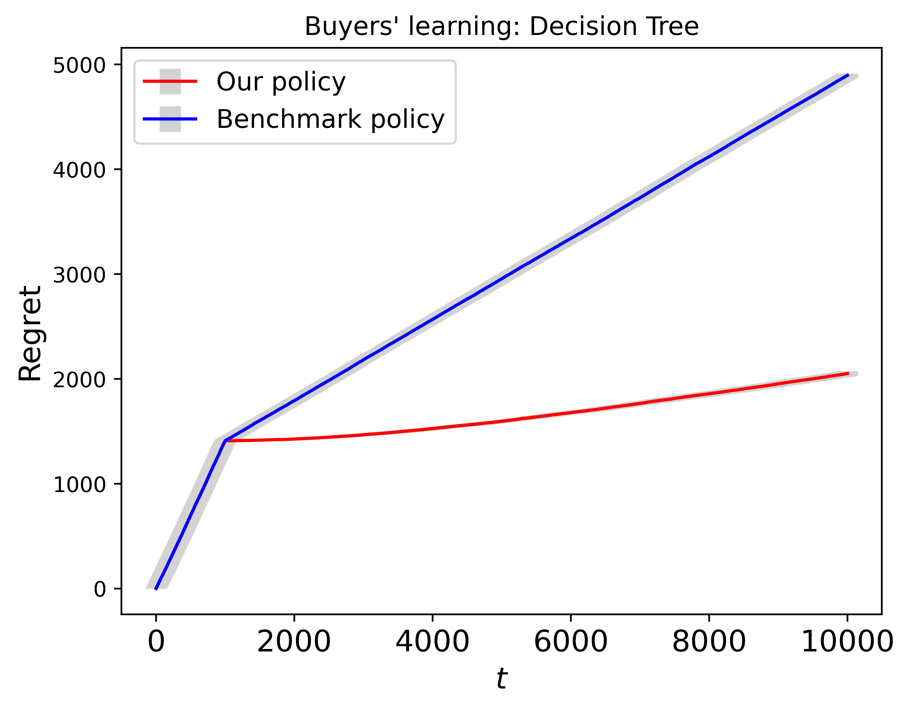
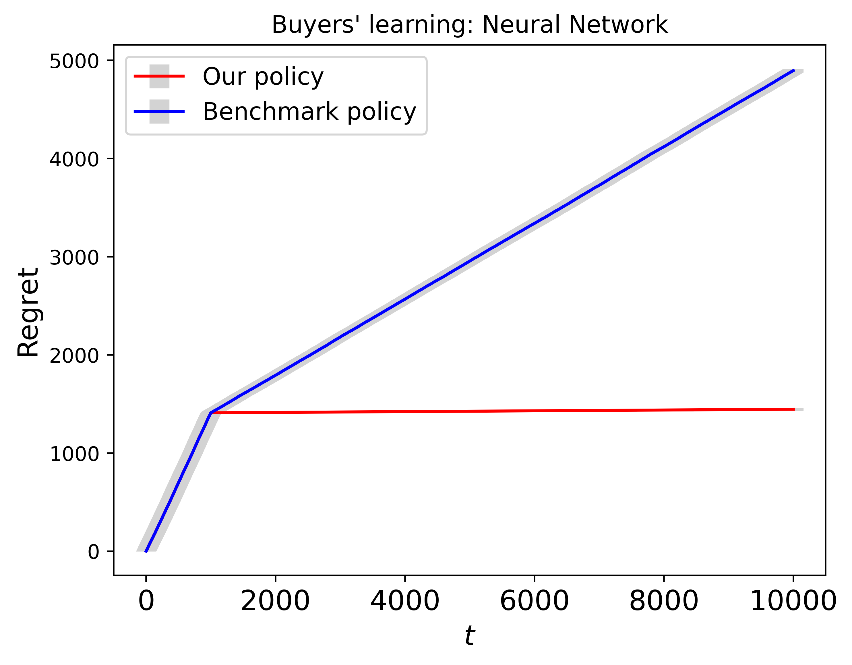
Figure 2: Regret plots for the two policies. The two subplots show the regrets of two different scenarios: decision tree regression and neural network. The red and blue lines represent the mean regret of our pricing policy and the benchmark pricing policy without buyers’ fairness learning, respectively, over 20 independent runs. The light gray areas around these lines depict the standard errors of the estimates.

5.2 Impacts of $d$ and $q$

In this section, we explore the impacts of the feature dimension $d\in\{3,10\}$ and the proportion of strategic buyers $q\in\{0.5,0.8\}$ on our proposed pricing policy. In the left sub-figure of Figure 3, we fix $q=0.5$ and vary the dimensions of feature as $d=3$ and $d=10\ (\bm{\beta}_{0}=(2,1/2,1,1,1/2,1/2,1/2,1/2,1/2,1/2,1/2)^{\top},\bm{\beta}_{1}=\bm{\beta}_{0}/2)$. We observe that our policy under the higher dimension incurs a higher regret. In the right sub-figure of Figure 3, the regret for $q=0.8$ is larger than that for $q=0.5$. When the proportion of the strategic buyers is smaller, manipulation behaviors occur less frequently, resulting in a lower regret. Besides, an equal proportion of two groups achieves the smallest average estimation error, leading to a lower regret. These observations align with the theoretical findings of Theorems 2.

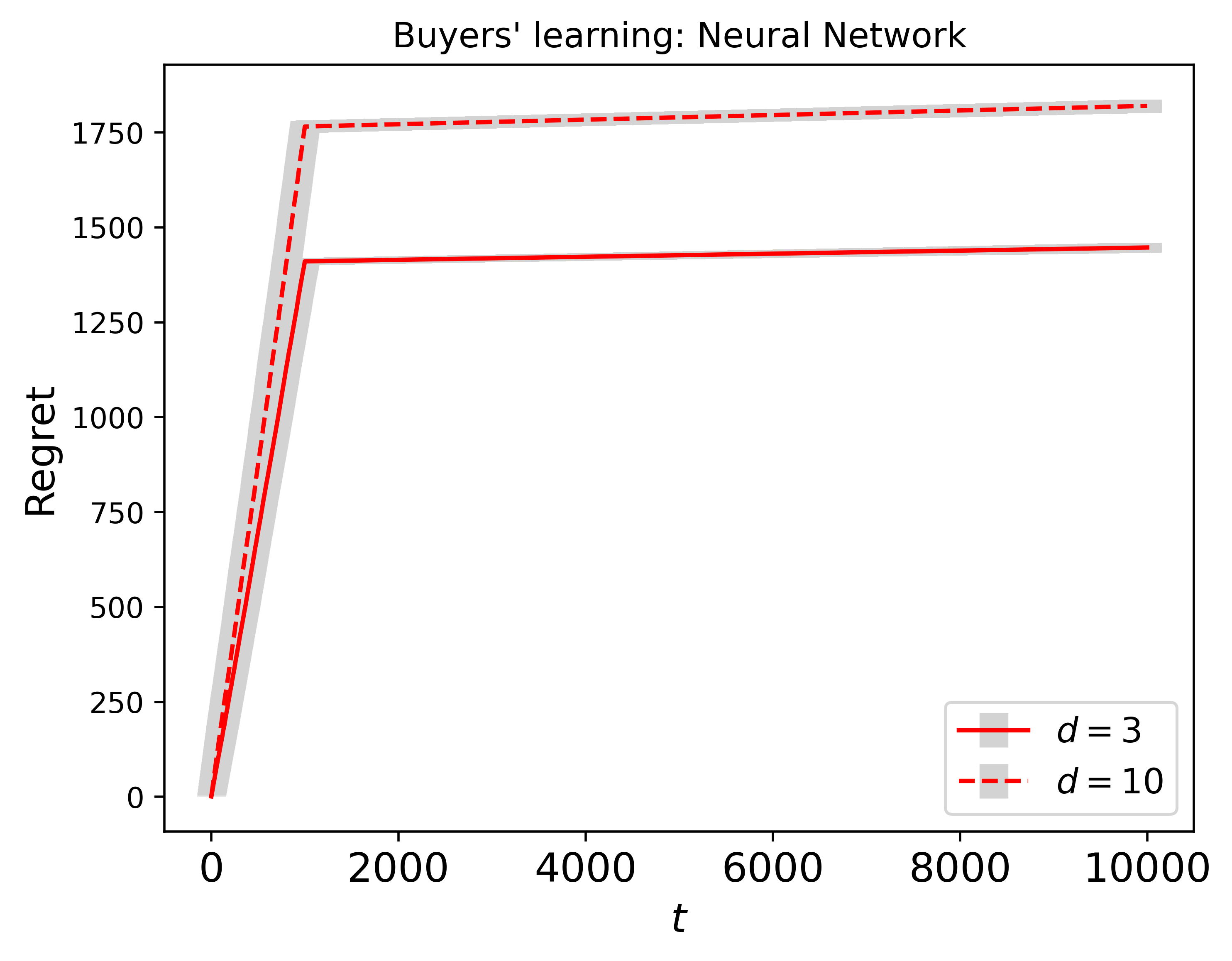
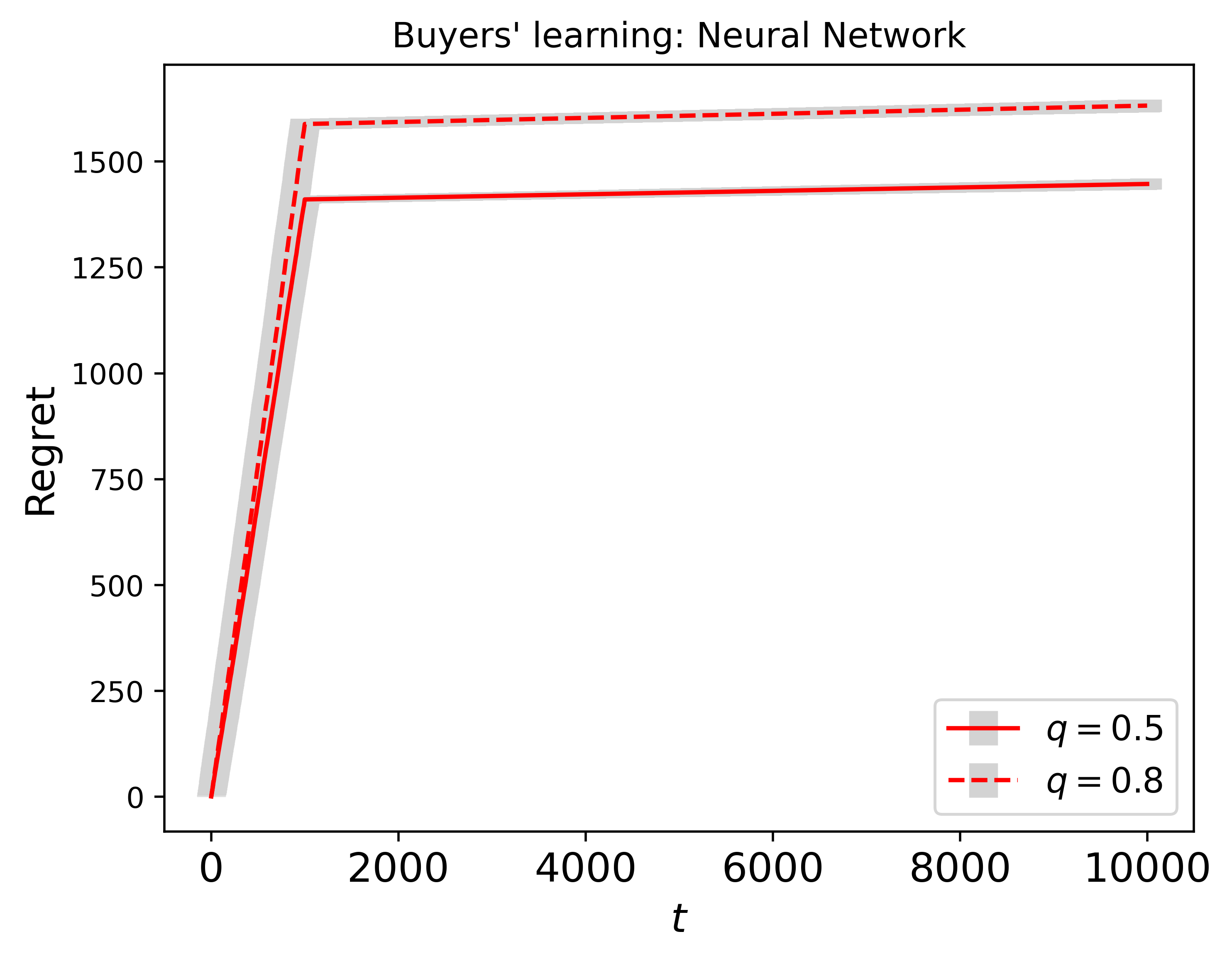
Figure 3: Regret plots for our policy. The two subplots show the regrets of the policy at different values of $d$ and $q$. The remaining caption is the same as Figure 2.

5.3 Sensitivity Tests

In this section, we investigate the sensitivity of our policy to hyperparameters $B,\tau,c_{\delta}$ required in Algorithm 1. Here, $B$ represents an upper bound on the price, and $\tau$ is a constant used in determining the exploration length, and $c_{\delta}$ is a parameter in our policy. To assess the sensitivity of our policies, we conduct experiments with different values of these hyperparameters in the setting with $q=0.5$.

First, we examine the sensitivity of $B$. For these simulations, we set $c_{\delta}=1$ and $\tau=10$. Figure 4 illustrates the regrets of the three policies under three scenarios: $B=3$, $B=4$ and $B=5$.

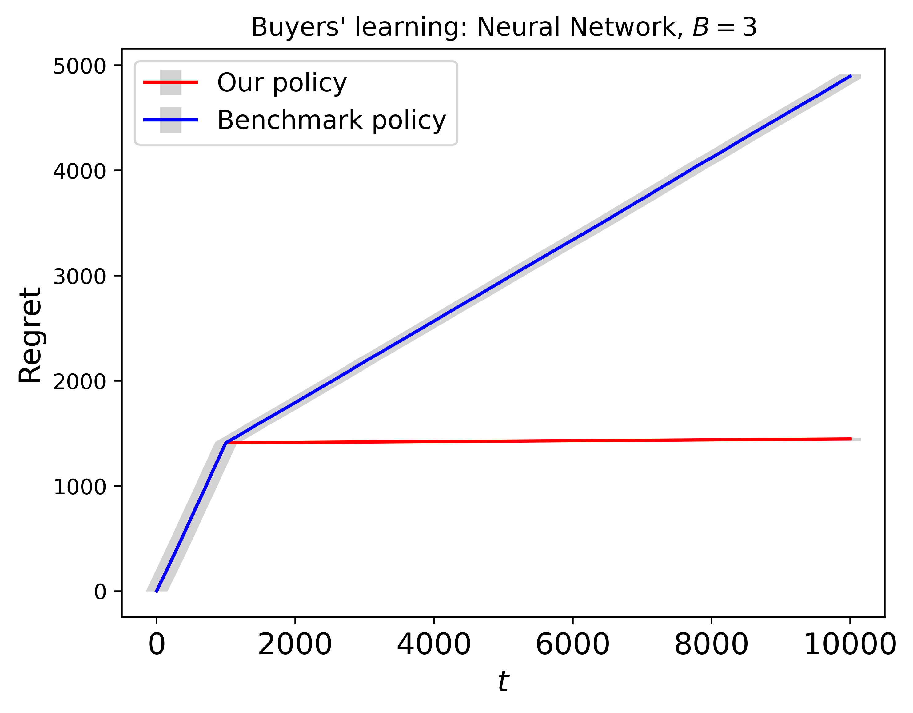
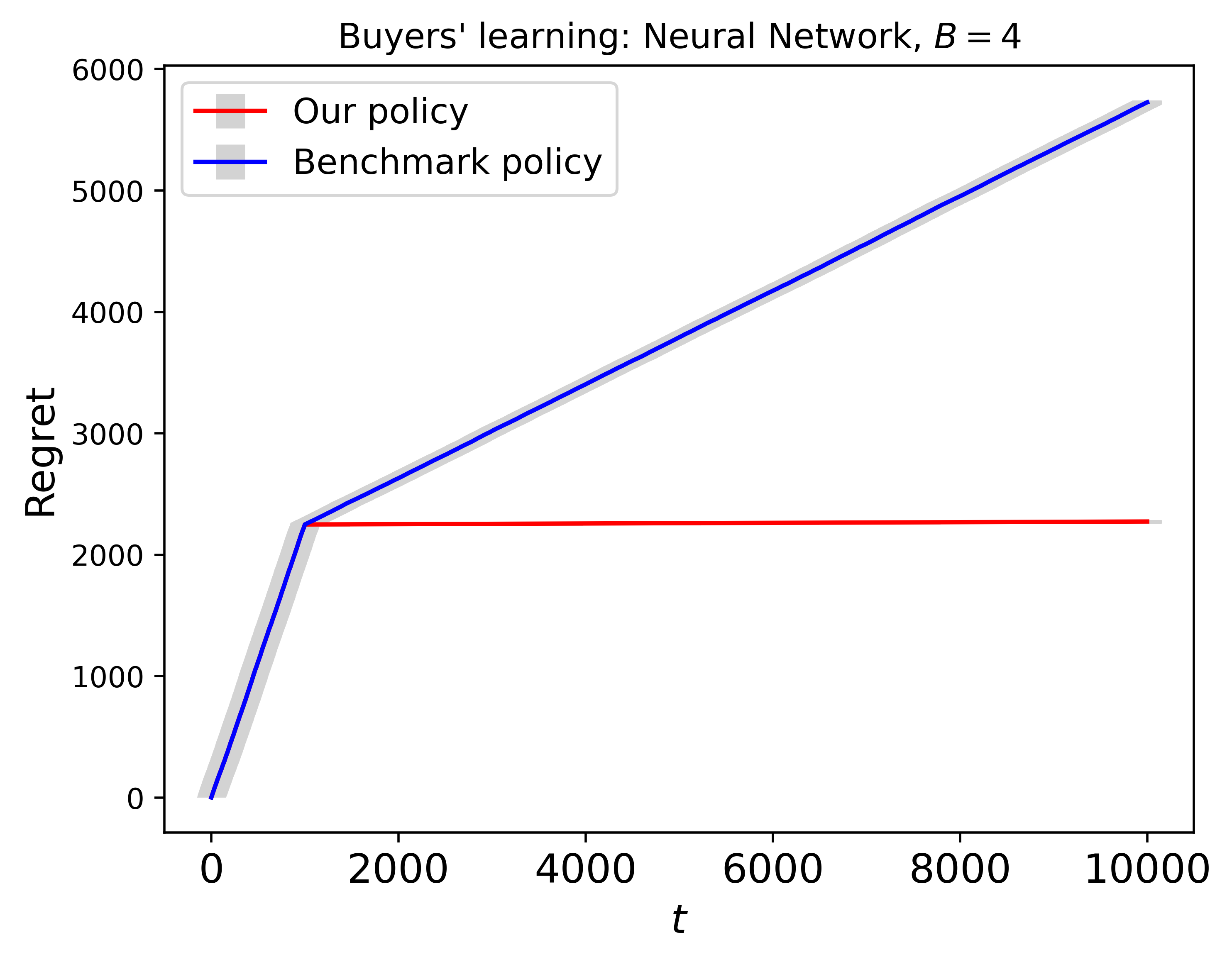
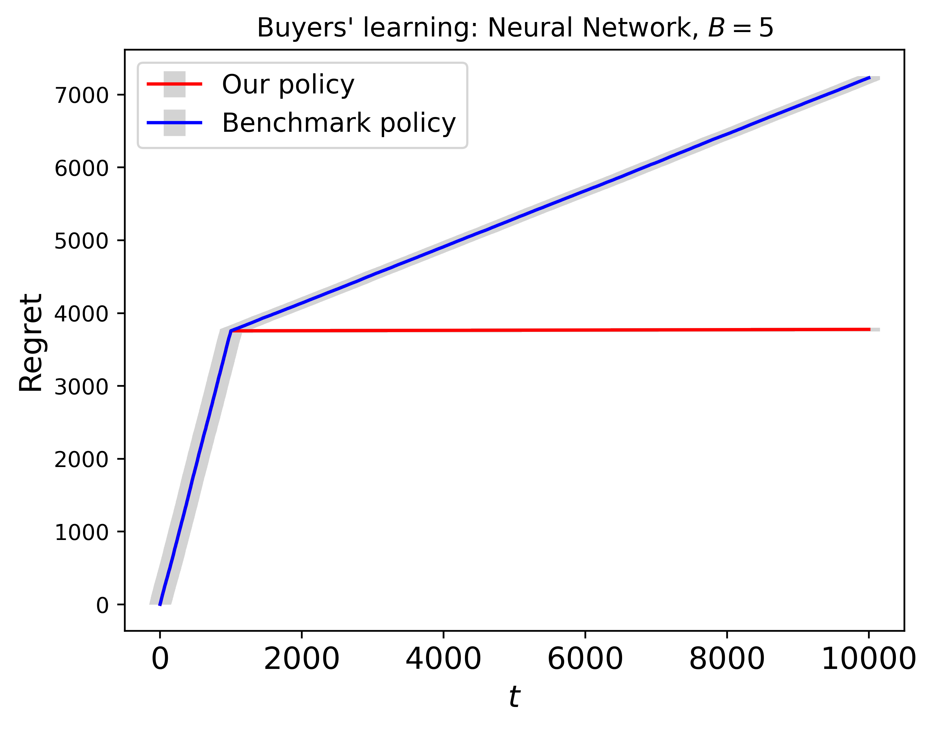
Figure 4: Regret plots for the two policies. The three subplots show the regrets of three different scenarios, $B\in\{3,4,5\}$. The remaining caption is the same as Figure 2.

Next, we examine the sensitivity of $c_{\delta}$. For these simulations, we set $B=3$ and $\tau=10$. Figure 5 illustrates the regrets of the three policies under three scenarios: $B=3$, $B=4$ and $B=5$.

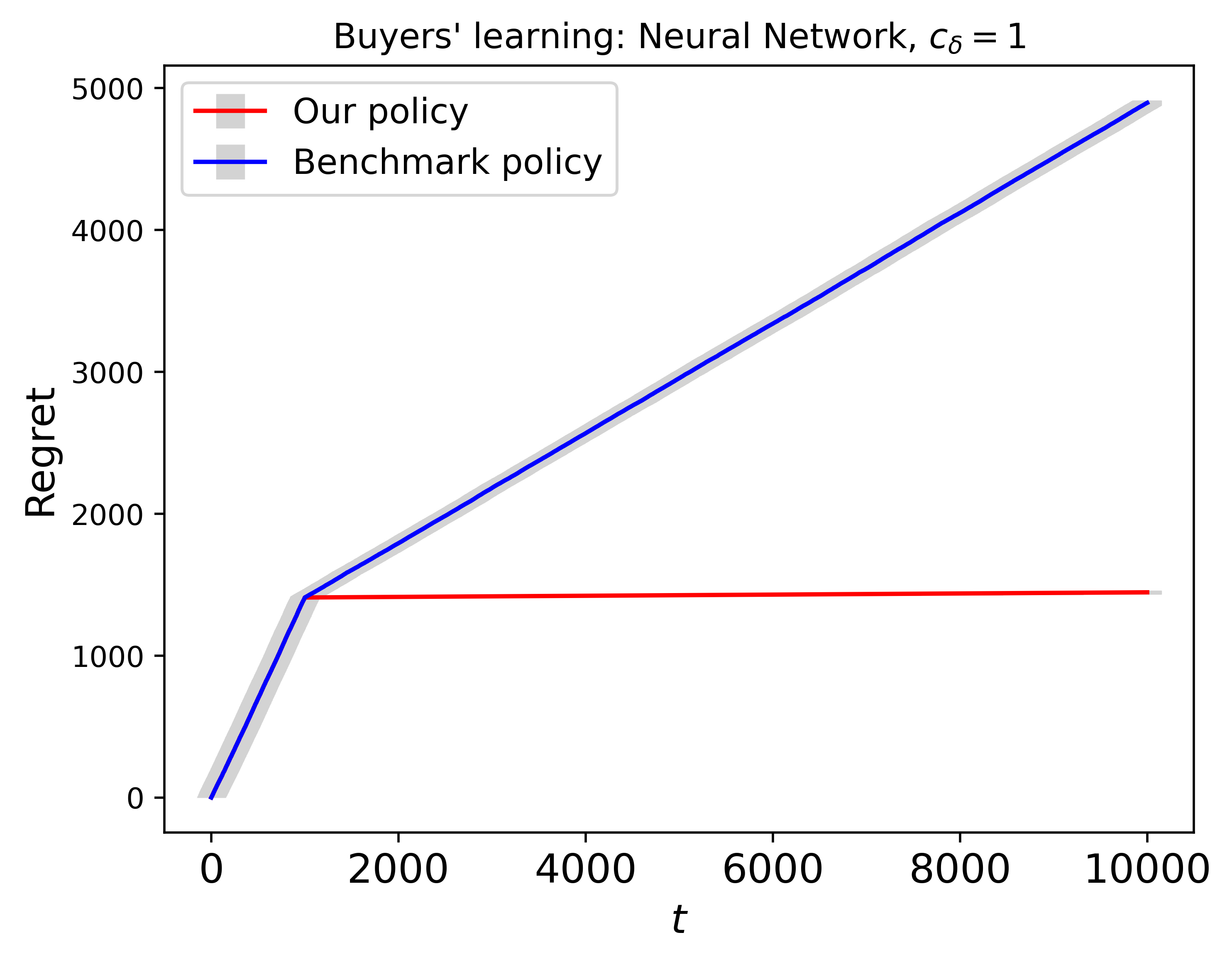
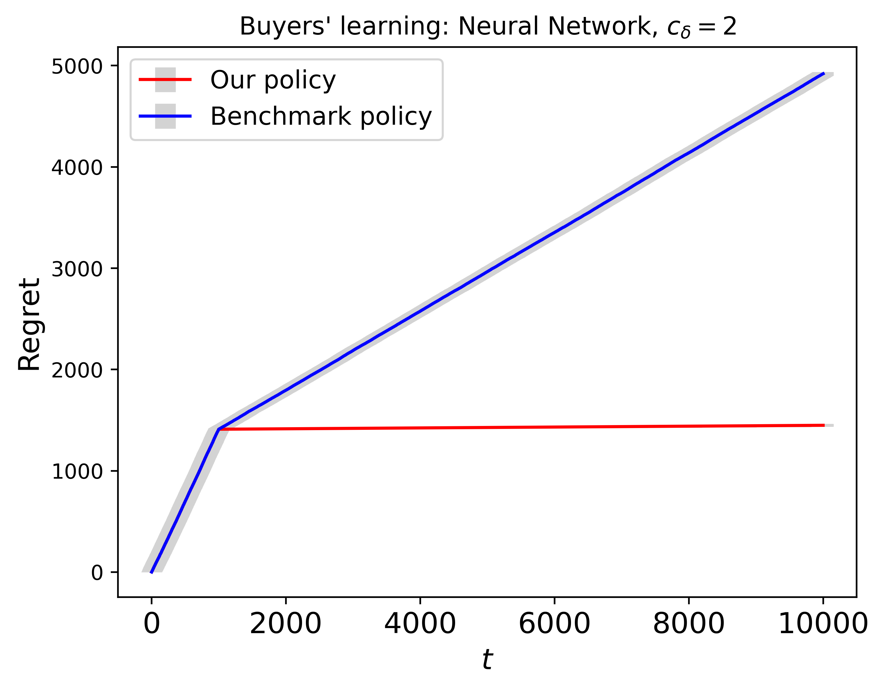
Figure 5: Regret plots for the two policies. The two subplots show the regrets of three different scenarios, $c_{\delta}\in\{1,2,3\}$. The remaining caption is the same as Figure 2.

Finally, we assess the sensitivity of $\tau$. In these simulations, we set $B=3$ and $c_{\delta}=1$. Figure 6 presents the regrets of the three policies for three different scenarios: $\tau=8$, $\tau=10$ and $\tau=12$.

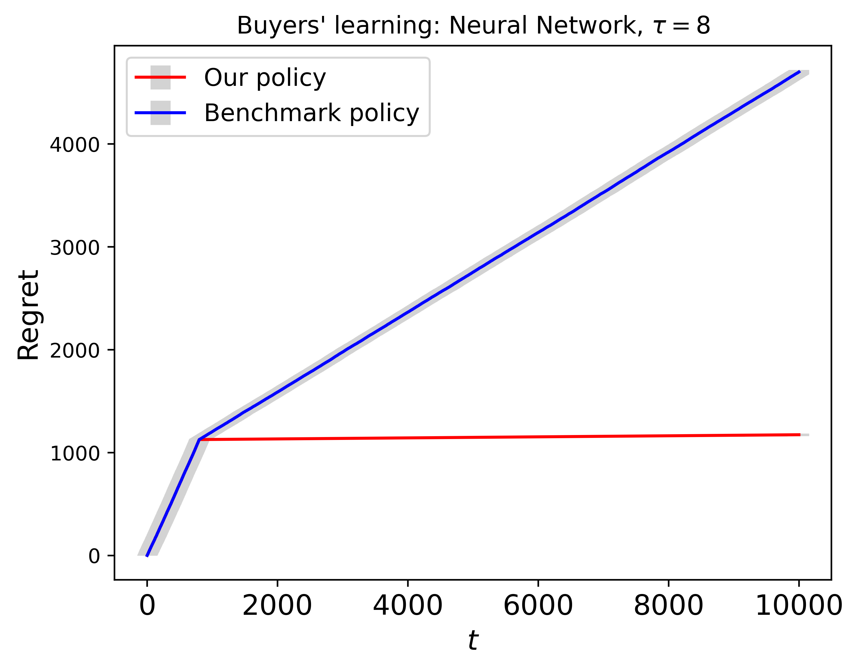
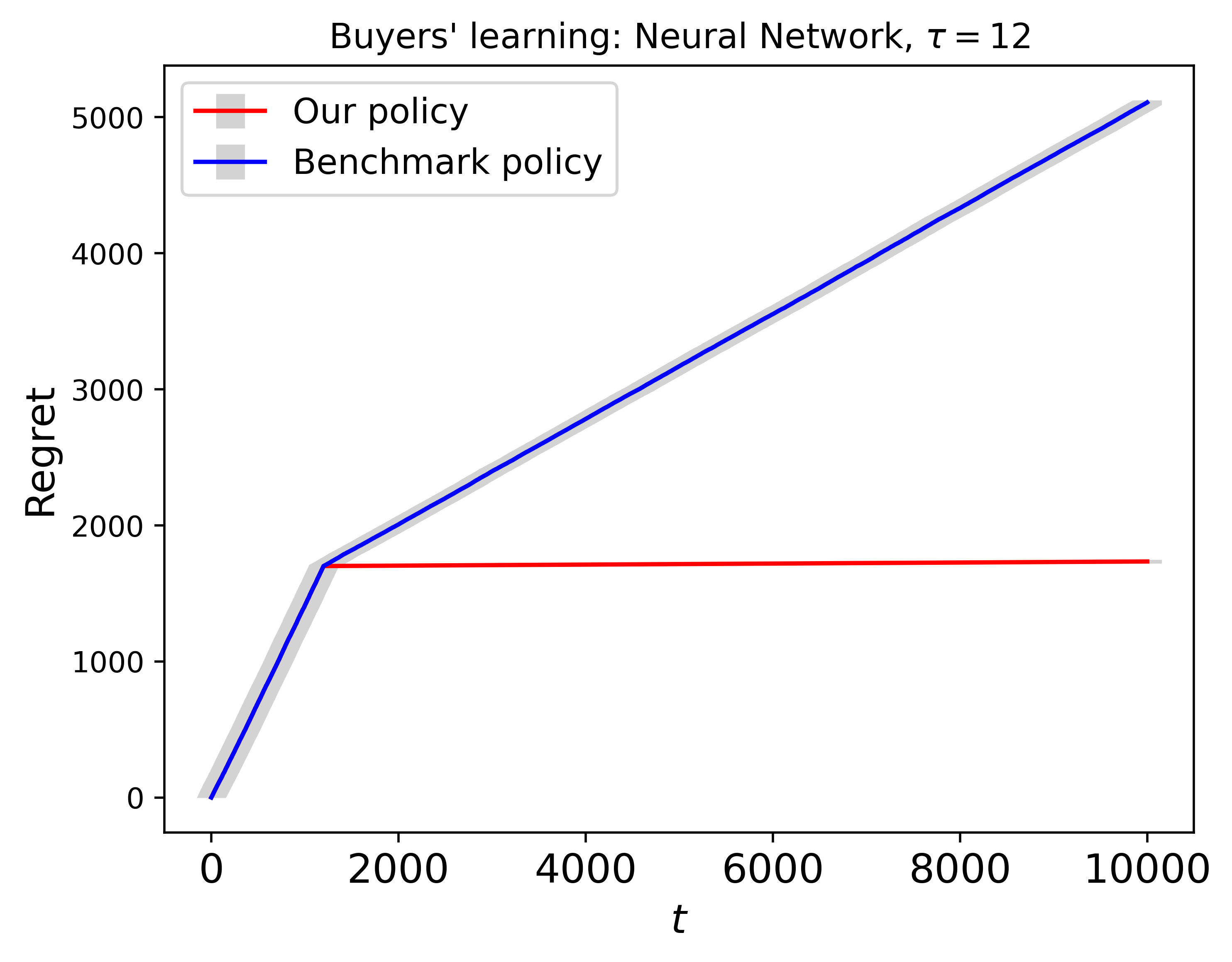
Figure 6: Regret plots for the two policies. The two subplots show the regrets of three different scenarios, $\tau\in\{8,10,12\}$. The remaining caption is the same as Figure 2.

Overall, our sensitivity analysis indicates that the performance of our policy remains consistent and robust under variations in the hyperparameters $B$, $c_{\delta},\tau$, and is always superior over the benchmark policy.

6 Real Application

In this section, we evaluate the efficacy of our policy using the public Home Mortgage Disclosure Act (HMDA) dataset that includes customer characteristics and loan features. In our study, we employ the 2022 HMDA dataset. HMDA mandates that numerous financial institutions maintain, report, and publicly disclose mortgage-related information. This dataset has been a focal point of prior research (Bocian et al., 2008; Zhang, 2018; Bartlett et al., 2022; Popick, 2022; Butler et al., 2023), revealing that borrowers from minority groups often face higher interest rates even after accounting for contextual factors.

6.1 Data Description and Preprocessing

We only retain data for loans that have been approved and disbursed to borrowers. We designate race as the group status, loan amount as the demand, interest rate as the price, and contextual information comprises income, age, property value securing the loan, debt-to-income ratio, combined loan-to-value ratio, and loan term. Race is categorized into two groups: White and non-White, encompassing Black or African American, American Indian or Alaska Native, Native Hawaiian or Other Pacific Islander, Asian and other minority races. We consider borrowers aged between 25 and 74. Initially provided in discrete intervals, we transform age into continuous data by averaging within each interval. The debt-to-income ratio is limited to the range of 20% to 60%. To ensure data integrity, we eliminate outliers, excluding the upper 5% and lower 5% of values, for loan amount, interest rate, income, property value, combined loan-to-value ratio, and loan term. Following data preprocessing, our dataset comprises 3,871,912 records. Among them, the White group constitutes 81.86% of the dataset.

6.2 Data Analysis

Before applying our pricing policy on the dataset, we employ the propensity score matching method (Ho et al., 2007, 2011) to examine the interest rate difference between the White group and the non-White group after controlling the contextual information. Let $\bar{p}_{0}$ and $\bar{p}_{1}$ be the mean prices of the non-White group and White group, respective. We test the hypothesis

$$H_{0}:\bar{p}_{1}=\bar{p}_{0},\ H_{1}:\bar{p}_{1}<\bar{p}_{0}.$$ (9)

The $p$-value of the hypothesis problem (9) is $2.2\times 10^{-16}$, indicating that the non-White group pays a higher interest rate compared to their White counterparts. This finding aligns with previous research (Bocian et al., 2008; Zhang, 2018; Bartlett et al., 2022; Popick, 2022; Butler et al., 2023).

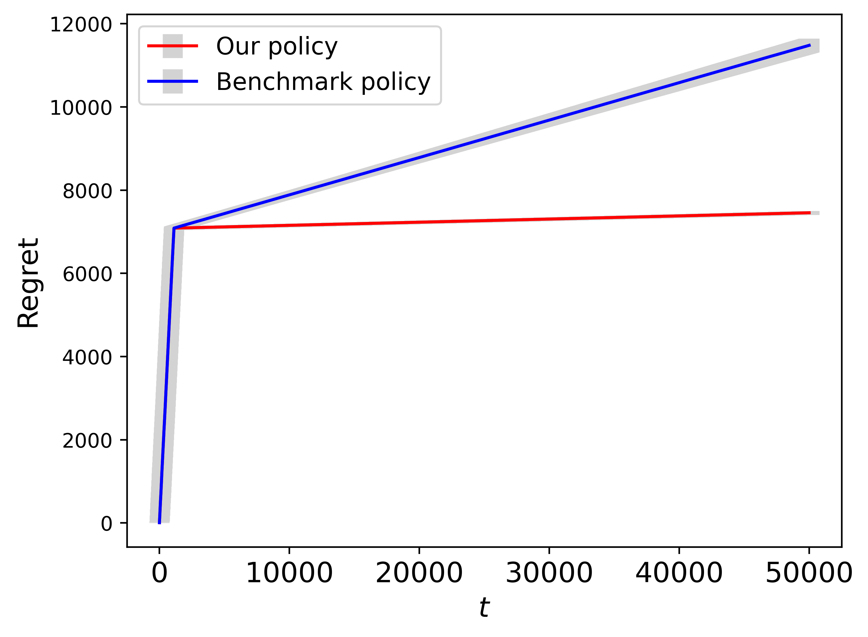
Figure 7: Regret plots for the two policies on the real data. The remaining caption is the same as Figure 2.

Now, we analyze the dataset using our online pricing policy. In practice, obtaining real-time feedback from buyers regarding any dynamic pricing strategy is challenging until the pricing policy has been executed in the data collection system. Consequently, we adhere to the calibration approach outlined in previous studies (Fan et al., 2024; Wang et al., 2024; Liu et al., 2024) by initially estimating a linear demand model. This model serves as a ground truth to evaluate dynamic pricing policies. We set the manipulation cost at $C_{0}=0.11$ and the fairness threshold to $\delta=0.1$. We assume $\epsilon_{t}\sim N(0,1)$, and fix $B=1$ and $\tau=5$. Buyers learn the price difference using a neural network. Our policy is applied with the time horizon $T=50000$ , repeated 20 times to record average cumulative regrets. We compare our policy against the benchmark pricing policy without considering buyers’ fairness learning. Figure 7 shows that the cumulative regret of the policy without buyers’ learning is much larger and grows significantly faster compared to our pricing policy, aligning with our earlier findings in simulated data. Our proposed pricing policy achieves 35.06% reduction in regret compared to the benchmark policy at the end of the time horizon.

7 Summary and Future Directions

In this paper, we study the contextual dynamic pricing problem when significant price disparities emerge among specific demographic groups such as gender or race. These disparities not only lead to legal concerns, but also incentivize disadvantaged buyers to strategically manipulate their group identity to obtain lower prices, further complicating the fairness landscape. To tackle these challenges, we propose a fairness-aware contextual dynamic pricing policy, considering scenarios where buyers’ group status is private and unobservable by the seller. Our policy addresses both price fairness and strategic behavior, simultaneously.

Looking ahead, there are several promising avenues for future exploration in this area. We can extend our investigation to incorporate additional complexities such as strategic pricing problems with censored demand (Tang et al., 2025), unobserved confounding (Yu et al., 2022; Miao et al., 2023; Qi et al., 2024; Shi et al., 2024), offline learning (Duan et al., 2021; Duan and Wainwright, 2024) and other fairness constraints (Fang et al., 2023). Exploring these avenues will aid in developing more robust and equitable dynamic pricing strategies for online retail environments.

In this supplement, we provide the detailed proofs. Section S.1 derives the solution of the optimization. Section S.2 gives the proof under the pricing policy without fairness learning, i.e., Theorem 1. Section S.3 and S.4 provide the proofs for Lemma 1 and Lemma 2. Section S.5 offers the proof for the upper regret bound of our proposed pricing policy, i.e., Theorem 2. Section S.6 presents the proof for Theorem 3, establishing a lower regret bound of any pricing policy in our problem. Section S.7 includes the supporting technical lemmas.

Appendix S.1 Derivation of (3)

The optimization problem (2) is equivalent to

$$\mathop{\min}_{p_{0},p_{1}} \ -qR_{0}(p_{0},\bm{x}_{t})-(1-q)R_{1}(p_{1},\bm{x}_{t})$$

$$s.t.\ p_{0}-p_{1}-\delta\leq 0.$$

The Lagrangian function is

$$\mathcal{L}(p_{0},p_{1},\lambda) =-qR_{0}(p_{0},\bm{x}_{t})-(1-q)R_{1}(p_{1},\bm{x}_{t})+\lambda(p_{0}-p_{1}-\delta)$$

$$=-q[p_{0}(\alpha_{0}p_{0}+\bm{\beta}_{0}^{\top}\widetilde{\bm{x}}_{t})]-(1-q)[p_{1}(\alpha_{1}p_{1}+\bm{\beta}_{1}^{\top}\widetilde{\bm{x}}_{t})]+\lambda(p_{0}-p_{1}-\delta).$$

By the Karush–Kuhn–Tucker condition, we have

$$\frac{\partial\mathcal{L}(p_{0},p_{1},\lambda)}{\partial p_{0}}=-2q\alpha_{0}p_{0}-q\bm{\beta}_{0}^{\top}\widetilde{\bm{x}}_{t}+\lambda=0,$$ (S1)

$$\frac{\partial\mathcal{L}(p_{0},p_{1},\lambda)}{\partial p_{1}}=-2(1-q)\alpha_{1}p_{1}-(1-q)\bm{\beta}_{1}^{\top}\widetilde{\bm{x}}_{t}-\lambda=0,$$

$$\lambda(p_{0}-p_{1}-\delta)=0,$$

$$p_{0}-p_{1}-\delta\leq 0,$$

$$\lambda\geq 0.$$

By solving (S1), we obtain

$$p_{j}^{*}(\bm{x}_{t})=\left\{\begin{aligned} &-\frac{\bm{\beta}_{j}^{\top}\widetilde{\bm{x}}_{t}}{2\alpha_{j}},&\text{if}\ \ \frac{\bm{\beta}_{1}^{\top}\widetilde{\bm{x}}_{t}}{2\alpha_{1}}-\frac{\bm{\beta}_{0}^{\top}\widetilde{\bm{x}}_{t}}{2\alpha_{0}}\leq\delta,\\ &\bm{\gamma}_{1}^{\top}\widetilde{\bm{x}}_{t}-j\cdot\delta+\gamma_{2},&\text{if}\ \ \frac{\bm{\beta}_{1}^{\top}\widetilde{\bm{x}}_{t}}{2\alpha_{1}}-\frac{\bm{\beta}_{0}^{\top}\widetilde{\bm{x}}_{t}}{2\alpha_{0}}>\delta,\end{aligned}\right.$$

where

$$\bm{\gamma}_{1}=-\frac{q\bm{\beta}_{0}+(1-q)\bm{\beta}_{1}}{2q\alpha_{0}+2(1-q)\alpha_{1}},\ \gamma_{2}=\frac{(1-q)\alpha_{1}\delta}{q\alpha_{0}+(1-q)\alpha_{1}}.$$

Appendix S.2 Proof of Theorem 1

We assume that the dimension of the features is $d=1$, and the expected demands of group 0 and group are $\mathbb{E}y_{0t}=2+x_{t}-p_{0t}$ and $\mathbb{E}y_{1t}=2+x_{t}-2p_{1t}$, respectively. We assume $x_{t}\sim$ Unif(-1/2, 1/2) and set $q=1/2,\delta=1/4$. By (3), the optimal prices for group 0 and group 1 under the fairness constraint are $p_{0}^{*}(x_{t})=x_{t}/3+5/6$ and $p_{1}^{*}(x_{t})=x_{t}/3+7/12$, respectively. We denote $p_{jt}^{*}=p_{jt}^{*}(\bm{x}_{t})$ and $p_{jt}=p_{jt}(\bm{x}_{t})$ for $j=0,1.$. The revenue of the optimal pricing policy at time $t$ under the fairness constraint is

$$\frac{1}{2}[R_{0}(p_{0t}^{*},x_{t})+R_{1}(p_{1t}^{*},x_{t})] =\frac{1}{2}[p_{0t}^{*}(x_{t}-p_{0t}^{*})+p_{1t}^{*}(x_{t}-2p_{1t}^{*})]$$ (S2)

$$=\frac{1}{2}\left(\frac{x_{t}}{3}+\frac{5}{6}\right)\left(\frac{2x_{t}}{3}+\frac{7}{6}\right)+\left(\frac{x_{t}}{3}+\frac{7}{12}\right)\left(\frac{x_{t}}{3}+\frac{5}{6}\right)$$

$$=\frac{x_{t}^{2}}{6}+\frac{17x_{t}}{24}+\frac{35}{48}.$$

Without the price fairness constraint, the optimal prices for group 0 and group 1 are $p_{0}^{\#}(x_{t})=(2+x_{t})/2$ and $p_{1}^{\#}(x_{t})=(2+x_{t})/4$, respectively. We set the manipulation cost as $C_{0}=5/16$. We have $p_{0}^{\#}(x_{t})-p_{1}^{\#}(x_{t})>C_{0}$. Since the buyers cannot perceive the price fairness, the buyers from group 0 consistently misreport their group status, leading to a payment of $p_{1}(x_{t})$. Therefore, the revenue of any other pricing policy without fairness learning at time $t$ is

$$\frac{1}{2}[R_{0}(p_{1t},x_{t})+R_{1}(p_{1t},x_{t})]=\frac{1}{2}[p_{1t}(2+x_{t}-p_{1t})+p_{1t}(2+x_{t}-2p_{1t})]\leq\frac{(2+x_{t})^{2}}{6}.$$ (S3)

By (S2) and (S3), the expected cumulative regret of any other pricing policy without fairness learning at time $T$ is

$$Regret_{T} =\frac{1}{2}\sum_{t=1}^{T}\mathbb{E}\{[R_{0}(p_{0t}^{*},x_{t})+R_{1}(p_{1t}^{*},x_{t})]-[R_{0}(p_{1t},x_{t})+R_{1}(p_{1t},x_{t})]\}$$

$$\leq\sum_{t=1}^{T}\mathbb{E}\left[\frac{x_{t}^{2}}{6}+\frac{17x_{t}}{24}+\frac{35}{48}-\frac{(2+x_{t})^{2}}{6}\right]$$

$$\leq\frac{T}{16}.$$

The proof is completed.

Appendix S.3 Proof of Lemma 1

Since the proofs for the estimation errors of $\bm{\theta}_{0}$ and $\bm{\theta}_{1}$ are identical, we omit the group symbol in the following proof, assuming that all variables are from the same group. To facilitate the presentation of the proof, we introduce some new notations. Let $\widetilde{p}_{t}=(1\ p_{t})^{\top}\in\mathbb{R}^{2}$ and $z_{t}=(\widetilde{p}_{t}^{\top}\ \bm{x}_{t}^{\top})^{\top}\in\mathbb{R}^{d+2}$. The prices and features from time 1 to $t$ are formulated as $Z_{t}=(z_{1},\cdots,z_{t})^{\top}\in\mathbb{R}^{t\times(d+2)}$, the demand is $Y_{t}=(y_{1},\cdots,y_{t})^{\top}\in\mathbb{R}^{t}$, and the noise sequence is $\bm{\epsilon}_{t}=(\epsilon_{1},\cdots,\epsilon_{t})^{\top}\in\mathbb{R}^{t}$. Therefore, the demand can be expressed as $Y_{t}=Z_{t}\bm{\theta}+\bm{\epsilon}_{t}$.

The OLS estimator of $\bm{\theta}$ is denoted as $\widehat{\bm{\theta}}=(Z_{t}^{\top}Z_{t})^{-1}Z_{t}^{\top}Y_{t}$. The estimation error of the parameter $\bm{\theta}$ is given by

$$\|\bm{\theta}-\widehat{\bm{\theta}}\|_{2}^{2}=\|(Z_{t}^{\top}Z_{t})^{-1}Z_{t}^{\top}\bm{\epsilon}_{t}\|_{2}^{2}=\bm{\epsilon}_{t}^{\top}Z_{t}(Z_{t}^{\top}Z_{t})^{-2}Z_{t}^{\top}\bm{\epsilon}_{t}\leq\frac{\bm{\epsilon}_{t}^{\top}Z_{t}Z_{t}^{\top}\bm{\epsilon}_{t}}{\lambda^{2}_{min}(Z_{t}^{\top}Z_{t})},$$ (S4)

where $\lambda_{min}(Z_{t}^{\top}Z_{t})$ is the minimum eigenvalue of the matrix $Z_{t}^{\top}Z_{t}$. To prove Lemma 1, we first establish an upper bound of $\lambda_{min}(Z_{t}^{\top}Z_{t})$ using the following lemma.

Lemma S3.

Let Assumptions 1 and 2 hold. Assume that $p_{1},\cdots,p_{t}$ are $i.i.d.$ from a uniform distribution $U(0,B)$, $\bm{x}_{1},\cdots,\bm{x}_{t}$ are $i.i.d.$ samples from an unknown distribution with $\mathbb{E}\bm{x}_{i}=\bm{0}$, and $p_{i}$ is independent from $\bm{x}_{i}$. Then, with a probability of at least $1-(d+2)(\frac{e}{2})^{-\frac{\lambda_{0}t}{2L}}$, the minimum eigenvalue of $Z_{t}^{\top}Z_{t}=\sum_{i=1}^{t}z_{i}z_{i}^{\top}$ is given by

$$\lambda_{min}(Z_{t}^{\top}Z_{t})\geq\frac{\lambda_{0}t}{2},$$

where

$$\lambda_{0}=\mathop{\min}\bigg{\{}\frac{B^{2}+3-\sqrt{B^{4}+3B^{2}+9}}{6},\lambda_{min}(\Sigma_{x})\bigg{\}}\textit{and}\ L=B^{2}+1+x_{max}^{2}.$$

Proof.

Note that $p_{i}$ is independent of $\bm{x}_{i}$. This together with the fact that $\mathbb{E}\bm{x}_{i}=\bm{0}$ leads to the conclusion $\mathbb{E}(p_{i}\bm{x}_{i})=\mathbb{E}p_{i}\mathbb{E}(\bm{x}_{i})=\bm{0}$. Using $z_{i}=(\widetilde{p}_{i}^{\top}\ \bm{x}_{i}^{\top})^{\top}$, we obtain

$$\mathbb{E}z_{i}z_{i}^{\top}=\begin{pmatrix}\mathbb{E}\widetilde{p}_{i}\widetilde{p}_{i}^{\top}&\mathbb{E}\widetilde{p}_{i}\bm{x}_{i}^{\top}\\ \mathbb{E}\bm{x}_{i}\widetilde{p}_{i}^{\top}&\mathbb{E}\bm{x}_{i}\bm{x}_{i}^{\top}\end{pmatrix}=\begin{pmatrix}\mathbb{E}\widetilde{p}_{i}\widetilde{p}_{i}^{\top}&\bm{0}^{\top}\\ \bm{0}&\Sigma_{x}\end{pmatrix}.$$

Recall that $\widetilde{p}_{t}=(1\ p_{t})^{\top}$. Given that $p_{i}$ follows a uniform distribution $U(0,B)$, we have

$$\mathbb{E}\widetilde{p}_{i}\widetilde{p}_{i}^{\top}=\begin{pmatrix}1&\mathbb{E}p_{i}\\ \mathbb{E}p_{i}&\mathbb{E}p_{i}^{2}\end{pmatrix}=\begin{pmatrix}1&B/2\\ B/2&B^{2}/3\end{pmatrix}.$$

By simple calculation, the minimum eigenvalue of $\mathbb{E}\widetilde{p}_{i}\widetilde{p}_{i}^{\top}$ is $\lambda_{min}(\mathbb{E}\widetilde{p}_{i}\widetilde{p}_{i}^{\top})=\frac{B^{2}+3-\sqrt{B^{4}+3B^{2}+9}}{6}>0$. Consequently, the minimum eigenvalue of $\mathbb{E}z_{i}z_{i}^{\top}$ can be expressed as

$$\lambda_{min}(\mathbb{E}z_{i}z_{i}^{\top}) =\mathop{\min}\{\lambda_{min}(\mathbb{E}\widetilde{p}_{i}\widetilde{p}_{i}^{\top}),\lambda_{min}(\Sigma_{x})\}=\mathop{\min}\bigg{\{}\frac{B^{2}+3-\sqrt{B^{4}+3B^{2}+9}}{6},\lambda_{min}(\Sigma_{x})\bigg{\}}.$$

Under Assumption 2, we know $\lambda_{min}(\Sigma_{x})>0$. Thus, $\lambda_{0}>0$. Because $\{z_{i}z_{i}^{\top}\}_{i=1}^{t}$ are $i.i.d.$, we have

$$\lambda_{min}\left(\sum_{i=1}^{t}\mathbb{E}z_{i}z_{i}^{\top}\right)=\lambda_{min}(t\mathbb{E}z_{i}z_{i}^{\top})=t\lambda_{min}(\mathbb{E}z_{i}z_{i}^{\top})=\lambda_{0}t.$$

According to Assumption 1, the maximum eigenvalue of $z_{i}z_{i}^{\top}$ is

$$\lambda_{max}(z_{i}z_{i}^{\top}) =tr(z_{i}^{\top}z_{i})=1+p_{i}^{2}+\|\bm{x}_{i}\|_{2}^{2}\leq B^{2}+1+x_{max}^{2}:=L.$$

Obviously, $\{z_{i}z_{i}^{\top}\}_{i=1}^{t}$ are independent, random, self-adjoint matrices with dimension $d+2$. According to Lemma S9 and the fact that each matrix $z_{i}z_{i}^{\top}$ is positive semi-definite, with $\zeta=1/2$, we have

$$\mathbb{P}\bigg{\{}\lambda_{min}\bigg{(}\sum_{i=1}^{t}z_{i}z_{i}^{\top}\bigg{)}\leq\frac{\lambda_{0}t}{2}\bigg{\}}\leq(d+2)\bigg{(}\frac{e}{2}\bigg{)}^{-\frac{\lambda_{0}t}{2L}}.$$

This completes the proof. ∎

We now return to the proof of Lemma 1. During the exploration phase, the price $p_{i}$ is $i.i.d.$ from $U(0,B)$, and the feature $\bm{x}_{i}$ is $i.i.d.$, with $p_{i}$ being independent from $\bm{x}_{i}$. Utilizing Lemma S3, we observe that

$$\mathbb{P}\bigg{(}\lambda_{min}(Z_{t}^{\top}Z_{t})>\frac{\lambda_{0}t}{2}\bigg{)}\geq 1-(d+2)\bigg{(}\frac{e}{2}\bigg{)}^{-\frac{\lambda_{0}t}{2L}}.$$ (S5)

Next, we establish an upper bound for $\bm{\epsilon}_{t}^{\top}Z_{t}Z_{t}^{\top}\bm{\epsilon}_{t}$. By Assumption 1, we have $\|\bm{\theta}-\widehat{\bm{\theta}}\|_{2}^{2}\leq 2(a_{max}^{2}+b_{max}^{2})$. Using (S4) and (S5), the expectation of the estimation error of $\bm{\theta}$ is given by

$$\mathbb{E}(\|\bm{\theta}-\widehat{\bm{\theta}}\|_{2}^{2}) =\mathbb{E}[\|\bm{\theta}-\widehat{\bm{\theta}}\|_{2}^{2}I(\lambda_{min}(Z_{t}^{\top}Z_{t})\geq\frac{\lambda_{0}t}{2})]+\mathbb{E}[\|\bm{\theta}-\widehat{\bm{\theta}}\|_{2}^{2}I(\lambda_{min}(Z_{t}^{\top}Z_{t})<\frac{\lambda_{0}t}{2})]$$ (S6)

$$\leq\mathbb{E}\bigg{[}\frac{\|Z_{t}^{\top}\bm{\epsilon}_{t}\|_{2}^{2}I(\lambda_{min}(Z_{t}^{\top}Z_{t})\geq\lambda_{0}t/2)}{\lambda_{min}^{2}(Z_{t}^{\top}Z_{t})}\bigg{]}+2(a_{max}^{2}+b_{max}^{2})\mathbb{P}\bigg{(}\lambda_{min}^{2}(Z_{t}^{\top}Z_{t})<\frac{\lambda_{0}t}{2}\bigg{)}$$

$$\leq\frac{4\mathbb{E}\|Z_{t}^{\top}\bm{\epsilon}_{t}\|_{2}^{2}}{\lambda_{0}^{2}t^{2}}+2(a_{max}^{2}+b_{max}^{2})(d+2)\bigg{(}\frac{e}{2}\bigg{)}^{-\frac{\lambda_{0}t}{2L}}.$$

Considering that $\epsilon_{i}$ is independent of $\epsilon_{j}$, $z_{i}$ and $z_{j}$ for $i\neq j$, and $\mathbb{E}\epsilon_{i}=0$, we have $\mathbb{E}(z_{i}^{\top}z_{j}\epsilon_{i}\epsilon_{j})=0$. Therefore,

$$\mathbb{E}\|Z_{t}^{\top}\bm{\epsilon}_{t}\|_{2}^{2}=\mathbb{E}\bigg{(}\sum_{i=1}^{t}z_{i}^{\top}z_{i}\epsilon_{i}^{2}\bigg{)}=\sigma_{\epsilon}^{2}\mathbb{E}\bigg{(}\sum_{i=1}^{t}z_{i}^{\top}z_{i}\bigg{)}\leq t\sigma_{\epsilon}^{2}(B^{2}+1+x_{max}^{2}).$$ (S7)

Combining (S6) and (S7), we have

$$\mathbb{E}(\|\bm{\theta}-\widehat{\bm{\theta}}\|_{2}^{2}) \leq\frac{4\sigma_{\epsilon}^{2}(B^{2}+1+x_{max}^{2})}{\lambda_{0}^{2}t}+2(a_{max}^{2}+b_{max}^{2})(d+2)\left(\frac{e}{2}\right)^{-\frac{\lambda_{0}t}{2L}}.$$

Noting that when $t\geq 6$, $(\frac{e}{2})^{-t}<\frac{1}{t}$. We have when $t\geq\frac{12L}{\lambda_{0}}$,

$$\mathbb{E}(\|\widehat{\bm{\theta}}-\bm{\theta}\|_{2}^{2})\leq\frac{4L[\sigma_{\epsilon}^{2}+\lambda_{0}(a_{max}^{2}+b_{max}^{2})(d+2)]}{\lambda_{0}^{2}t}.$$ (S8)

Since the length of the exploration phase is $T_{0}$ and the proportion of buyers from group 0 is $q$, the numbers of samples used to estimate $\bm{\theta}_{0}$ and $\bm{\theta}_{1}$ are $qT_{0}$ and $(1-q)T_{0}$, respectively. We substitute $t=qT_{0}$ and $t=(1-q)T_{0}$ into (S8) to obtain the estimation errors of $\bm{\theta}_{0}$ and $\bm{\theta}_{1}$. This concludes the proof.

Appendix S.4 Proof of Lemma 2

Let $p_{0}(\cdot)$ and $p_{1}(\cdot)$ be the pricing functions in (8). When $\frac{\widehat{\bm{\beta}}_{1}^{\top}\widetilde{\bm{x}}_{t}}{2\widehat{\alpha}_{1}}-\frac{\widehat{\bm{\beta}}_{0}^{\top}\widetilde{\bm{x}}_{t}}{2\widehat{\alpha}_{0}}\leq\delta-c_{\delta}\sqrt{\frac{\log T_{0}}{T_{0}}}$, the price difference is

$$\widehat{\delta} =\widehat{p}_{0}(\bm{x})-\widehat{p}_{1}(\bm{x})$$

$$=\widehat{p}_{0}(\bm{x})-p_{0}(\bm{x})+p_{1}(\bm{x})-\widehat{p}_{1}(\bm{x})+p_{0}(\bm{x})-p_{1}(\bm{x})$$

$$=\widehat{p}_{0}(\bm{x})-p_{0}(\bm{x})+p_{1}(\bm{x})-\widehat{p}_{1}(\bm{x})+\frac{\widehat{\bm{\beta}}_{1}^{\top}\widetilde{\bm{x}}_{t}}{2\widehat{\alpha}_{1}}-\frac{\widehat{\bm{\beta}}_{0}^{\top}\widetilde{\bm{x}}_{t}}{2\widehat{\alpha}_{0}}-\delta+\delta$$

$$\leq\widehat{p}_{0}(\bm{x})-p_{0}(\bm{x})+p_{1}(\bm{x})-\widehat{p}_{1}(\bm{x})-c_{\delta}\sqrt{\frac{\log T_{0}}{T_{0}}}+\delta.$$

Therefore,

$$\widehat{\delta}-C_{0}\leq\widehat{p}_{0}(\bm{x})-p_{0}(\bm{x})+p_{1}(\bm{x})-\widehat{p}_{1}(\bm{x})-c_{\delta}\sqrt{\frac{\log T_{0}}{T_{0}}}+\delta-C_{0}$$ (S9)

When $\frac{\widehat{\bm{\beta}}_{1}^{\top}\widetilde{\bm{x}}_{t}}{2\widehat{\alpha}_{1}}-\frac{\widehat{\bm{\beta}}_{0}^{\top}\widetilde{\bm{x}}_{t}}{2\widehat{\alpha}_{0}}>\delta-c_{\delta}\sqrt{\frac{\log T_{0}}{T_{0}}}$, the price difference is

$$\widehat{\delta} =\widehat{p}_{0}(\bm{x})-\widehat{p}_{1}(\bm{x})$$

$$=\widehat{p}_{0}(\bm{x})-p_{0}(\bm{x})+p_{1}(\bm{x})-\widehat{p}_{1}(\bm{x})+p_{0}(\bm{x})-p_{1}(\bm{x})$$

$$=\widehat{p}_{0}(\bm{x})-p_{0}(\bm{x})+p_{1}(\bm{x})-\widehat{p}_{1}(\bm{x})+\delta.$$

Therefore,

$$\widehat{\delta}-C_{0}=\widehat{p}_{0}(\bm{x})-p_{0}(\bm{x})+p_{1}(\bm{x})-\widehat{p}_{1}(\bm{x})+\delta-C_{0}$$ (S10)

By (S9) and (S10), we have

$$\widehat{\delta}-C_{0}\leq\widehat{p}_{0}(\bm{x})-p_{0}(\bm{x})+p_{1}(\bm{x})-\widehat{p}_{1}(\bm{x})+\delta-C_{0}.$$

At time $t$, buyers learn the price difference $\widehat{\delta}$ using $t-1$ samples. By Assumption 3, with at least probability $1-2\eta_{t-1}$, we have $|\widehat{p}_{0}(\bm{x})-p_{0}(\bm{x})|\leq\mathcal{E}_{\mathcal{P},\eta_{t-1}}(t-1)$ and $|p_{1}(\bm{x})-\widehat{p}_{1}(\bm{x})|\leq\mathcal{E}_{\mathcal{P},\eta_{t-1}}(t-1)$. Therefore, with at least probability $1-2\eta_{t-1}$,

$$\widehat{\delta}-C_{0}\leq 2\mathcal{E}_{\mathcal{P},\eta_{t-1}}(t-1)+\delta-C_{0}$$

Since $\mathcal{E}_{\mathcal{P},\eta_{t-1}}(t-1)$ decreases to 0 as $t$ increases, and $\Delta=\delta-C_{0}<0$ is a constant, when $t>c$ for some positive constant $c$, with at least probability $1-2\eta_{t-1}$, we have $\widehat{\delta}\leq C_{0}$.

Appendix S.5 Proof of Theorem 2

The time period is segmented into the exploration phase and the exploitation phase. The seller’s revenue at time $t$ is $R_{j}(p_{t})=R_{j}(p_{t},\bm{x}_{t})$ for $j=0,1$. Let

$$reg_{t}=qR_{0}(p^{*}_{0t})+(1-q)R_{1}(p^{*}_{1t})-qR_{0}(p_{0t})-(1-q)R_{1}(p_{1t})$$

be the regret under Algorithm 1 at time period $t$. by Assumption 1, we have

$$qR_{0}(p^{*}_{0t})+(1-q)R_{1}(p^{*}_{1t})-qR_{0}(p_{0t})-(1-q)R_{1}(p_{1t})\leq 2B(a_{max}B+b_{max}x_{max}).$$ (S11)

Therefore, the regret at time $t$ in the exploration phase is

$$\mathbb{E}(reg_{t})\leq 2B(a_{max}B+b_{max}x_{max}).$$ (S12)

Now, we focus on the analysis of the regret during the exploitation phase. During the exploitation phase, The pricing function (8) is equivalent to

$$p_{t}=\left\{\begin{aligned} &-\frac{\widehat{\bm{\beta}}_{G_{t}^{\prime}}^{\top}\widetilde{\bm{x}}_{t}}{2\widehat{\alpha}_{G_{t}^{\prime}}},&&\text{if}\ \ \frac{\widehat{\bm{\beta}}_{1}^{\top}\widetilde{\bm{x}}_{t}}{2\widehat{\alpha}_{1}}-\frac{\widehat{\bm{\beta}}_{0}^{\top}\widetilde{\bm{x}}_{t}}{2\widehat{\alpha}_{0}}\leq\delta-c_{\delta}\sqrt{\frac{\log T_{0}}{T_{0}}},\\ &\widehat{\bm{\gamma}}_{1}^{\top}\widetilde{\bm{x}}_{t}-\delta\cdot G_{t}^{\prime}+\widehat{\gamma}_{2},&&\text{if}\ \ \frac{\widehat{\bm{\beta}}_{1}^{\top}\widetilde{\bm{x}}_{t}}{2\widehat{\alpha}_{1}}-\frac{\widehat{\bm{\beta}}_{0}^{\top}\widetilde{\bm{x}}_{t}}{2\widehat{\alpha}_{0}}\geq\delta+c_{\delta}\sqrt{\frac{\log T_{0}}{T_{0}}},\\ &\widehat{\bm{\gamma}}_{1}^{\top}\widetilde{\bm{x}}_{t}-\delta\cdot G_{t}^{\prime}+\widehat{\gamma}_{2},&&\text{if}\ \ \delta-c_{\delta}\sqrt{\frac{\log T_{0}}{T_{0}}}<\frac{\widehat{\bm{\beta}}_{1}^{\top}\widetilde{\bm{x}}_{t}}{2\widehat{\alpha}_{1}}-\frac{\widehat{\bm{\beta}}_{0}^{\top}\widetilde{\bm{x}}_{t}}{2\widehat{\alpha}_{0}}<\delta+c_{\delta}\sqrt{\frac{\log T_{0}}{T_{0}}}.\end{aligned}\right.$$ (S13)

We now show that the probability $\mathbb{P}\left(\delta-c_{\delta}\sqrt{\frac{\log T_{0}}{T_{0}}}<\frac{\widehat{\bm{\beta}}_{1}^{\top}\widetilde{\bm{x}}_{t}}{2\widehat{\alpha}_{1}}-\frac{\widehat{\bm{\beta}}_{0}^{\top}\widetilde{\bm{x}}_{t}}{2\widehat{\alpha}_{0}}<\delta+c_{\delta}\sqrt{\frac{\log T_{0}}{T_{0}}}\right)$ is small using the following lemma.

Lemma S4.

There exists some positive constant $c_{1}$, such that when $T_{0}>c_{1}$,

$$\mathbb{P}\left(\delta-c_{\delta}\sqrt{\frac{\log T_{0}}{T_{0}}}<\frac{\widehat{\bm{\beta}}_{1}^{\top}\widetilde{\bm{x}}_{t}}{2\widehat{\alpha}_{1}}-\frac{\widehat{\bm{\beta}}_{0}^{\top}\widetilde{\bm{x}}_{t}}{2\widehat{\alpha}_{0}}<\delta+c_{\delta}\sqrt{\frac{\log T_{0}}{T_{0}}}\right)\leq\frac{4}{T_{0}}+(d+2)[(\frac{e}{2})^{-\frac{\lambda_{0}qT_{0}}{2L}}+(\frac{e}{2})^{-\frac{\lambda_{0}(1-q)T_{0}}{2L}}].$$

Proof.

We denote $\Delta_{\bm{x}_{t}}=\frac{\bm{\beta}_{0}^{\top}\widetilde{\bm{x}}_{t}}{2\alpha_{0}}-\frac{\bm{\beta}_{1}^{\top}\widetilde{\bm{x}}_{t}}{2\alpha_{1}}+\delta$. Then

$$~~~~\mathbb{P}\left(\delta-c_{\delta}\sqrt{\frac{\log T_{0}}{T_{0}}}<\frac{\widehat{\bm{\beta}}_{1}^{\top}\widetilde{\bm{x}}_{t}}{2\widehat{\alpha}_{1}}-\frac{\widehat{\bm{\beta}}_{0}^{\top}\widetilde{\bm{x}}_{t}}{2\widehat{\alpha}_{0}}<\delta+c_{\delta}\sqrt{\frac{\log T_{0}}{T_{0}}}\right)$$ (S14)

$$=\mathbb{P}\left(\delta-c_{\delta}\sqrt{\frac{\log T_{0}}{T_{0}}}<\frac{\widehat{\bm{\beta}}_{1}^{\top}\widetilde{\bm{x}}_{t}}{2\widehat{\alpha}_{1}}-\frac{\bm{\beta}_{1}^{\top}\widetilde{\bm{x}}_{t}}{2\alpha_{1}}+\frac{\bm{\beta}_{0}^{\top}\widetilde{\bm{x}}_{t}}{2\alpha_{0}}-\frac{\widehat{\bm{\beta}}_{0}^{\top}\widetilde{\bm{x}}_{t}}{2\widehat{\alpha}_{0}}+\frac{\bm{\beta}_{1}^{\top}\widetilde{\bm{x}}_{t}}{2\alpha_{1}}-\frac{\bm{\beta}_{0}^{\top}\widetilde{\bm{x}}_{t}}{2\alpha_{0}}<\delta+c_{\delta}\sqrt{\frac{\log T_{0}}{T_{0}}}\right)$$

$$=\mathbb{P}\left(\Delta_{\bm{x}_{t}}-c_{\delta}\sqrt{\frac{\log T_{0}}{T_{0}}}<\frac{\widehat{\bm{\beta}}_{1}^{\top}\widetilde{\bm{x}}_{t}}{2\widehat{\alpha}_{1}}-\frac{\bm{\beta}_{1}^{\top}\widetilde{\bm{x}}_{t}}{2\alpha_{1}}+\frac{\bm{\beta}_{0}^{\top}\widetilde{\bm{x}}_{t}}{2\alpha_{0}}-\frac{\widehat{\bm{\beta}}_{0}^{\top}\widetilde{\bm{x}}_{t}}{2\widehat{\alpha}_{0}}<\Delta_{\bm{x}_{t}}+c_{\delta}\sqrt{\frac{\log T_{0}}{T_{0}}}\right).$$

There exists some positive constant $c_{1}$ such that $\Delta_{\bm{x}_{t}}>2c_{\delta}\sqrt{\frac{\log T_{0}}{T_{0}}}$ when $T_{0}>c_{1}$. For any $T_{0}>c_{1}$, by (S14), we have

$$~~~~\mathbb{P}\left(\delta-c_{\delta}\sqrt{\frac{\log T_{0}}{T_{0}}}<\frac{\widehat{\bm{\beta}}_{1}^{\top}\widetilde{\bm{x}}_{t}}{2\widehat{\alpha}_{1}}-\frac{\widehat{\bm{\beta}}_{0}^{\top}\widetilde{\bm{x}}_{t}}{2\widehat{\alpha}_{0}}<\delta+c_{\delta}\sqrt{\frac{\log T_{0}}{T_{0}}}\right)$$

$$\leq\mathbb{P}\left(\frac{\widehat{\bm{\beta}}_{1}^{\top}\widetilde{x}_{t}}{2\widehat{\alpha}_{1}}-\frac{\bm{\beta}_{1}^{\top}\widetilde{\bm{x}}_{t}}{2\alpha_{1}}+\frac{\bm{\beta}_{0}^{\top}\widetilde{\bm{x}}_{t}}{2\alpha_{0}}-\frac{\widehat{\bm{\beta}}_{0}^{\top}\widetilde{\bm{x}}_{t}}{2\widehat{\alpha}_{0}}>\Delta_{\bm{x}_{t}}-c_{\delta}\sqrt{\frac{\log T_{0}}{T_{0}}}\right)$$

$$\leq\mathbb{P}\left(\left(\frac{\widehat{\bm{\beta}}_{1}^{\top}\widetilde{\bm{x}}_{t}}{2\widehat{\alpha}_{1}}-\frac{\bm{\beta}_{1}^{\top}\widetilde{\bm{x}}_{t}}{2\alpha_{1}}+\frac{\bm{\beta}_{0}^{\top}\widetilde{\bm{x}}_{t}}{2\alpha_{0}}-\frac{\widehat{\bm{\beta}}_{0}^{\top}\widetilde{\bm{x}}_{t}}{2\widehat{\alpha}_{0}}\right)^{2}>\left(\Delta_{\bm{x}_{t}}-c_{\delta}\sqrt{\frac{\log T_{0}}{T_{0}}}\right)^{2}\right)$$

$$\leq\mathbb{P}\left(\left(\frac{\widehat{\bm{\beta}}_{1}^{\top}\widetilde{\bm{x}}_{t}}{2\widehat{\alpha}_{1}}-\frac{\bm{\beta}_{1}^{\top}\widetilde{\bm{x}}_{t}}{2\alpha_{1}}+\frac{\bm{\beta}_{0}^{\top}\widetilde{\bm{x}}_{t}}{2\alpha_{0}}-\frac{\widehat{\bm{\beta}}_{0}^{\top}\widetilde{\bm{x}}_{t}}{2\widehat{\alpha}_{0}}\right)^{2}>\frac{c^{2}_{\delta}\log T_{0}}{T_{0}}\right).$$

Next, we have

$$\left(\frac{\widehat{\bm{\beta}}_{1}^{\top}\widetilde{\bm{x}}_{t}}{2\widehat{\alpha}_{1}}-\frac{\bm{\beta}_{1}^{\top}\widetilde{\bm{x}}_{t}}{2\alpha_{1}}+\frac{\bm{\beta}_{0}^{\top}\widetilde{\bm{x}}_{t}}{2\alpha_{0}}-\frac{\widehat{\bm{\beta}}_{0}^{\top}\widetilde{\bm{x}}_{t}}{2\widehat{\alpha}_{0}}\right)^{2} \leq 2\left(\frac{\widehat{\bm{\beta}}_{0}^{\top}\widetilde{\bm{x}}_{t}}{2\widehat{\alpha}_{0}}-\frac{\bm{\beta}_{0}^{\top}\widetilde{\bm{x}}_{t}}{2\alpha_{0}}\right)^{2}+2\left(\frac{\widehat{\bm{\beta}}_{1}^{\top}\widetilde{\bm{x}}_{t}}{2\widehat{\alpha}_{1}}-\frac{\bm{\beta}_{1}^{\top}\widetilde{\bm{x}}_{t}}{2\alpha_{1}}\right)^{2}$$ (S15)

$$\leq\frac{\mathop{\max}\{a_{max}^{2},b_{max}^{2}\}x_{max}^{2}\sum_{j=0}^{1}\|\widehat{\bm{\theta}}_{j}-\bm{\theta}_{j}\|_{2}^{2}}{a_{min}^{4}},$$

where the second inequality follows from

$$\left(\frac{\widehat{\bm{\beta}}_{j}^{\top}\widetilde{\bm{x}}_{t}}{2\widehat{\alpha}_{j}}-\frac{\bm{\beta}_{j}^{\top}\widetilde{\bm{x}}_{t}}{2\alpha_{j}}\right)^{2} =\left(\frac{\alpha_{j}\widehat{\bm{\beta}}_{j}^{\top}\widetilde{\bm{x}}_{t}-\widehat{\alpha}_{j}\bm{\beta}_{j}^{\top}\widetilde{\bm{x}}_{t}+\alpha_{j}\bm{\beta}_{j}^{\top}\widetilde{\bm{x}}_{t}-\alpha_{j}\bm{\beta}_{j}^{\top}\widetilde{\bm{x}}_{t}}{2\alpha_{j}\widehat{\alpha}_{j}}\right)^{2}$$

$$=\left(\frac{\alpha_{j}\widetilde{x}_{t}^{\top}(\widehat{\bm{\beta}}_{j}-\bm{\beta}_{j})+(\alpha_{j}-\widehat{\alpha}_{j})\bm{\beta}_{j}^{\top}\widetilde{\bm{x}}_{t}}{2\alpha_{j}\widehat{\alpha}_{j}}\right)^{2}$$

$$\leq\frac{2a_{max}^{2}x_{max}^{2}\|\widehat{\bm{\beta}}_{j}-\bm{\beta}_{j}\|_{2}^{2}+2b_{max}^{2}x_{max}^{2}\|\alpha_{j}-\widehat{\alpha}_{j}\|_{2}^{2}}{4a_{min}^{4}}$$

$$\leq\frac{\mathop{\max}\{a_{max}^{2},b_{max}^{2}\}x_{max}^{2}\|\widehat{\bm{\theta}}_{j}-\bm{\theta}_{j}\|_{2}^{2}}{2a_{min}^{4}}$$

by leveraging Assumption 1 for $j=0,1$.

Lemma S5.

Assume $0<\eta<1$. Let $T_{0}$ be the length of the exploration phase and $q$ be the proportion of buyers in group 0. $\widehat{\bm{\theta}}_{0}$ and $\widehat{\bm{\theta}}_{1}$ are obtained by (2). Under Assumptions 1 and 2, We have with probability at least $1-\eta-(d+2)(e/2)^{-\frac{\lambda_{0}qT_{0}}{2L}}$,

$$\|\widehat{\bm{\theta}}_{0}-\bm{\theta}_{0}\|_{2}^{2}\leq\frac{8(d+2)z_{max}^{2}\sigma_{\epsilon}^{2}\log(2/\eta)}{\lambda_{0}^{2}qT_{0}},$$

and with probability at least $1-\eta-(d+2)(e/2)^{-\frac{\lambda_{0}(1-q)T_{0}}{2L}}$,

$$\|\widehat{\bm{\theta}}_{1k}-\bm{\theta}_{1}\|_{2}^{2}\leq\frac{8(d+2)z_{max}^{2}\sigma_{\epsilon}^{2}\log(2/\eta)}{\lambda_{0}^{2}(1-q)T_{0}},$$

where $z_{max}=\mathop{\max}\{1,x_{max},B\}$, $\lambda_{0}=\mathop{\min}\{(B^{2}+3-\sqrt{B^{4}+3B^{2}+9})/6,\lambda_{min}(\Sigma_{x})\}$, and $L=B^{2}+1+x_{max}^{2}$.

Proof.

Recall that $Z_{t}=(z_{1},\cdots,z_{t})^{\top}\in\mathbb{R}^{t\times(d+2)}$ with $z_{t}=(1\ p_{t}\ \bm{x}_{t}^{\top})^{\top}\in\mathbb{R}^{d+2}$ from the exploration phase. We slightly abuse the notation and let $z_{ij}$ be the $(i,j)$-th elements of $Z_{t}$. Under Assumption 1, we have $|z_{ij}|\leq\mathop{\max}\{1,x_{max},B\}:=z_{max}$. Noting that $\epsilon_{i}$ is bounded independent $\sigma_{\epsilon}^{2}$-sub-Gaussian variable with mean zero, and $z_{ij}$ is independent from $\epsilon_{i}$, we know that $z_{ij}\epsilon_{i}$ is zero-mean bounded random variable with variance at most $z_{max}^{2}\sigma_{\epsilon}^{2}$. By Lemma S10, for $0<\eta_{j}<1$, we have

$$~~~~\mathbb{P}\bigg{(}\bigg{|}\sum_{i=1}^{t}z_{ij}\epsilon_{i}\bigg{|}<z_{max}\sigma_{\epsilon}\sqrt{2t\log(2/\eta_{j})}\bigg{)}$$ (S16)

$$=1-\mathbb{P}\bigg{(}\bigg{|}\sum_{i=1}^{t}z_{ij}\epsilon_{i}\bigg{|}\geq z_{max}\sigma_{\epsilon}\sqrt{2t\log(2/\eta_{j})}\bigg{)}$$

$$=1-\mathbb{P}\bigg{(}\sum_{i=1}^{t}z_{ij}\epsilon_{i}\geq z_{max}\sigma_{\epsilon}\sqrt{2t\log(2/\eta_{j})}\bigg{)}-\mathbb{P}\bigg{(}-\sum_{i=1}^{t}z_{ij}\epsilon_{i}\geq z_{max}\sigma_{\epsilon}\sqrt{2t\log(2/\eta_{j})}\bigg{)}$$

$$\geq 1-\eta_{j}.$$

Let $0<\eta<1$ and $\eta_{j}=\eta/(d+2)$ for $j=1,\cdots,(d+2)$. By (S16), with probability at least $1-\eta$, we have

$$\bm{\epsilon}_{t}^{\top}Z_{t}Z_{t}^{\top}\bm{\epsilon}_{t} =\sum_{j=1}^{d+2}\bigg{(}\sum_{i=1}^{t}z_{ij}\epsilon_{i}\bigg{)}^{2}\leq 2(d+2)z_{max}^{2}\sigma_{\epsilon}^{2}t\log(2/\eta).$$ (S17)

By (S4), (S5) and (S17), we see

$$\|\widehat{\bm{\theta}}-\bm{\theta}\|_{2}^{2}\leq\frac{\bm{\epsilon}_{t}^{\top}Z_{t}Z_{t}^{\top}\bm{\epsilon}_{t}}{\lambda^{2}_{min}(Z_{t}^{\top}Z_{t})}\leq\frac{8(d+2)z_{max}^{2}\sigma_{\epsilon}^{2}\log(2/\eta)}{\lambda_{0}^{2}t},$$ (S18)

with probability at least $1-\eta-(d+2)(e/2)^{-\frac{\lambda_{0}t}{2L}}$. Since the length of the exploration phase is $T_{0}$, and the proportion of buyers from group 0 is $q$, the numbers of samples used to estimate $\bm{\theta}_{0}$ and $\bm{\theta}_{1}$ are $qT_{0}$ and $(1-q)T_{0}$, respectively. Plugging $t=qT_{0}$ and $t=(1-q)T_{0}$ into (S18), respectively, we can obtain the estimation errors of $\bm{\theta}_{0}$ and $\bm{\theta}_{1}$. ∎

By Lemma S5 with $\eta=2/T_{0}$, we have with probability at most $\frac{4}{T_{0}}+(d+2)[(e/2)^{-\frac{\lambda_{0}qT_{0}}{2L}}+(e/2)^{-\frac{\lambda_{0}(1-q)T_{0}}{2L}}]$,

$$\frac{\mathop{\max}\{a_{max}^{2},b_{max}^{2}\}x_{max}^{2}\sum_{j=0}^{1}\|\widehat{\bm{\theta}}_{j}-\bm{\theta}_{j}\|_{2}^{2}}{a_{min}^{4}}>\frac{8(d+2)z_{max}^{2}\sigma_{\epsilon}^{2}\log(T_{0})\mathop{\max}\{a_{max}^{2},b_{max}^{2}\}x_{max}^{2}}{a_{min}^{4}\lambda_{0}^{2}q(1-q)T_{0}}.$$ (S19)

We denote $c_{\delta}=\sqrt{\frac{8(d+2)z_{max}^{2}\sigma_{\epsilon}^{2}\mathop{\max}\{a_{max}^{2},b_{max}^{2}\}x_{max}^{2}}{a_{min}^{4}\lambda_{0}^{2}q(1-q)}}$. Finally, we obtain

$$\mathbb{P}\left(\delta-c_{\delta}\sqrt{\frac{\log T_{0}}{T_{0}}}<\frac{\widehat{\bm{\beta}}_{1}^{\top}\widetilde{\bm{x}}_{t}}{2\widehat{\alpha}_{1}}-\frac{\widehat{\bm{\beta}}_{0}^{\top}\widetilde{\bm{x}}_{t}}{2\widehat{\alpha}_{0}}<\delta+c_{\delta}\sqrt{\frac{\log T_{0}}{T_{0}}}\right)\leq\frac{4}{T_{0}}+(d+2)[(\frac{e}{2})^{-\frac{\lambda_{0}qT_{0}}{2L}}+(\frac{e}{2})^{-\frac{\lambda_{0}(1-q)T_{0}}{2L}}].$$

∎

By Assumption 1, we have

$$\widehat{\bm{\gamma}}_{1}^{\top}\widetilde{\bm{x}}_{t}-\delta\cdot G_{t}^{\prime}+\widehat{\gamma}_{2}\leq\frac{b_{max}x_{max}+2a_{max}\delta}{2a_{min}}.$$ (S20)

Combining Lemma S4 and (S11), when $\delta-c_{\delta}\sqrt{\frac{\log T_{0}}{T_{0}}}<\frac{\widehat{\bm{\beta}}_{1}^{\top}\widetilde{\bm{x}}_{t}}{2\widehat{\alpha}_{1}}-\frac{\widehat{\bm{\beta}}_{0}^{\top}\widetilde{\bm{x}}_{t}}{2\widehat{\alpha}_{0}}<\delta+c_{\delta}\sqrt{\frac{\log T_{0}}{T_{0}}}$, the expected regret during the exploitation phase at time $t$ is given by

$$J_{0}:=\mathbb{E}(reg_{t}) \leq 2B(a_{max}B+b_{max}x_{max})\left\{\frac{4}{T_{0}}+(d+2)[(\frac{e}{2})^{-\frac{\lambda_{0}qT_{0}}{2L}}+(\frac{e}{2})^{-\frac{\lambda_{0}(1-q)T_{0}}{2L}}]\right\}$$ (S21)

$$\leq\frac{4B(a_{max}B+b_{max}x_{max})[(d+2)L+2\lambda_{0}q(1-q)]}{\lambda_{0}q(1-q)T_{0}},$$

where the inequality follows from the fact that when $T_{0}\geq 6,(e/2)^{-T_{0}}<1/T_{0}$.

Now, we start to analyze the cases where $\frac{\widehat{\bm{\beta}}_{1}^{\top}\widetilde{\bm{x}}_{t}}{2\widehat{\alpha}_{1}}-\frac{\widehat{\bm{\beta}}_{0}^{\top}\widetilde{\bm{x}}_{t}}{2\widehat{\alpha}_{0}}\leq\delta-c_{\delta}\sqrt{\frac{\log T_{0}}{T_{0}}}$ and $\frac{\widehat{\bm{\beta}}_{1}^{\top}\widetilde{\bm{x}}_{t}}{2\widehat{\alpha}_{1}}-\frac{\widehat{\bm{\beta}}_{0}^{\top}\widetilde{\bm{x}}_{t}}{2\widehat{\alpha}_{0}}\geq\delta+c_{\delta}\sqrt{\frac{\log T_{0}}{T_{0}}}$. Using the benchmark policy, the price for a buyer with features $\bm{x}_{t}$ from group $G_{t}=j\in\{0,1\}$ at time $t$ is determined by (3). By (S13), our policy is related to the disclosed group status $G_{t}^{\prime}$. Given the strategic nature of buyers, there exists the possibility of them revealing a false group status.

Given that the buyers from the group 1 (advantage group) do not manipulate and reveal the true group type, the price for these buyers under our policy is defined as

$$p_{1t}=\left\{\begin{aligned} &-\frac{\widehat{\bm{\beta}}_{1}^{\top}\widetilde{\bm{x}}_{t}}{2\widehat{\alpha}_{1}},&\text{if}\ \ \frac{\widehat{\bm{\beta}}_{1}^{\top}\widetilde{\bm{x}}_{t}}{2\widehat{\alpha}_{1}}-\frac{\widehat{\bm{\beta}}_{0}^{\top}\widetilde{\bm{x}}_{t}}{2\widehat{\alpha}_{0}}\leq\delta-c_{\delta}\sqrt{\frac{\log T_{0}}{T_{0}}},\\ &\widehat{\bm{\gamma}}_{1}^{\top}\widetilde{\bm{x}}_{t}-\delta+\widehat{\gamma}_{2},&\text{if}\ \ \frac{\widehat{\bm{\beta}}_{1}^{\top}\widetilde{\bm{x}}_{t}}{2\widehat{\alpha}_{1}}-\frac{\widehat{\bm{\beta}}_{0}^{\top}\widetilde{\bm{x}}_{t}}{2\widehat{\alpha}_{0}}\geq\delta+c_{\delta}\sqrt{\frac{\log T_{0}}{T_{0}}}.\end{aligned}\right.$$

The price for buyers from group 0 is contingent on the group status they reveal. Let $\widehat{\delta}$ be the price difference that the buyers in group 0 estimated based on the public data. If $\widehat{\delta}>C_{0}$, the buyers from group 0 reveal a manipulated group type. Conversely, if $\widehat{\delta}\leq C_{0}$, they disclose their true group type. Consequently, under our policy, the price for buyers in group 0 is given by

$$p_{0t}=\left\{\begin{array}[]{lr}p_{0t}^{\prime},\ \text{if}\ \widehat{\delta}\leq C_{0},\\ p_{1t},\ \text{if}\ \widehat{\delta}>C_{0},\end{array}\right.$$

where

$$p_{0t}^{\prime}=\left\{\begin{aligned} &-\frac{\widehat{\bm{\beta}}_{0}^{\top}\widetilde{\bm{x}}_{t}}{2\widehat{\alpha}_{0}},\ &\text{if}\ \ \frac{\widehat{\bm{\beta}}_{1}^{\top}\widetilde{\bm{x}}_{t}}{2\widehat{\alpha}_{1}}-\frac{\widehat{\bm{\beta}}_{0}^{\top}\widetilde{\bm{x}}_{t}}{2\widehat{\alpha}_{0}}\leq\delta-c_{\delta}\sqrt{\frac{\log T_{0}}{T_{0}}},\\ &\widehat{\bm{\gamma}}_{1}^{\top}\widetilde{\bm{x}}_{t}+\widehat{\gamma}_{2},\ &\text{if}\ \ \frac{\widehat{\bm{\beta}}_{1}^{\top}\widetilde{\bm{x}}_{t}}{2\widehat{\alpha}_{1}}-\frac{\widehat{\bm{\beta}}_{0}^{\top}\widetilde{\bm{x}}_{t}}{2\widehat{\alpha}_{0}}\geq\delta+c_{\delta}\sqrt{\frac{\log T_{0}}{T_{0}}}.\end{aligned}\right.$$

The regret of our policy depends on the probability $\mathbb{P}(\widehat{\delta}\leq C_{0})$. We define the historical information up to time $t$ as $\mathcal{H}_{t}=\{\bm{x}_{1},\cdots,\bm{x}_{t},y_{1},\cdots,y_{t},p_{1},\cdots,p_{t}\}$. We also define $\widetilde{\mathcal{H}}_{t}=\mathcal{H}_{t}\cup\{\bm{x}_{t+1}\}$ as the filtration including the feature $\bm{x}_{t+1}$. The expected regret at time $t$ in the exploitation phase is

$$\mathbb{E}(reg_{t}|\widetilde{\mathcal{H}}_{t-1}) =\mathbb{E}\{[qR_{0}(p^{*}_{0t})+(1-q)R_{1}(p^{*}_{1t})-qR_{0}(p_{0t})-(1-q)R_{1}(p_{1t})]|\widetilde{\mathcal{H}}_{t-1}\}\mathbb{I}(G_{t}=1)$$ (S22)

$$~~~+\mathbb{E}\{[qR_{0}(p^{*}_{0t})+(1-q)R_{1}(p^{*}_{1t})-qR_{0}(p_{0t})-(1-q)R_{1}(p_{1t})]|\widetilde{\mathcal{H}}_{t-1}\}\mathbb{I}(G_{t}=0)$$

$$=(1-q)\mathbb{E}\{[qR_{0}(p^{*}_{0t})+(1-q)R_{1}(p^{*}_{1t})-qR_{0}(p_{0t}^{\prime})-(1-q)R_{1}(p_{1t})]|\widetilde{\mathcal{H}}_{t-1}\}$$

$$~~~+q\mathbb{E}\{q[R_{0}(p^{*}_{0t})-R_{0}(p_{0t}^{\prime})]+(1-q)[R_{1}(p^{*}_{1t})-R_{1}(p_{1t})]|\widetilde{\mathcal{H}}_{t-1}\}\mathbb{P}(\widehat{\delta}\leq C_{0})$$

$$~~~+q\mathbb{E}\{q[R_{0}(p^{*}_{0t})-R_{0}(p_{1t})]+(1-q)[R_{1}(p^{*}_{1t})-R_{1}(p_{1t})]|\widetilde{\mathcal{H}}_{t-1}\}\mathbb{P}(\widehat{\delta}>C_{0})$$

$$\leq\underbrace{\mathbb{E}\{q[R_{0}(p^{*}_{0t})-R_{0}(p_{0t}^{\prime})]+(1-q)[R_{1}(p^{*}_{1t})-R_{1}(p_{1t})]|\widetilde{\mathcal{H}}_{t-1}\}}_{J_{1}}$$

$$~~~+\underbrace{q\mathbb{E}\{q[R_{0}(p^{*}_{0t})-R_{0}(p_{1t})]+(1-q)[R_{1}(p^{*}_{1t})-R_{1}(p_{1t})]|\widetilde{\mathcal{H}}_{t-1}\}\mathbb{P}(\widehat{\delta}>C_{0})}_{J_{2}}.$$

We first analyze $J_{1}$. For $J_{1}$, buyers report their true group status. We can rewrite $J_{1}$ as

$$J_{1} =\underbrace{J_{1}\mathbb{I}\left(\frac{\bm{\beta}_{1}^{\top}\widetilde{\bm{x}}_{t}}{2\alpha_{1}}-\frac{\bm{\beta}_{0}^{\top}\widetilde{\bm{x}}_{t}}{2\alpha_{0}}\geq\delta,\ \frac{\widehat{\bm{\beta}}_{1}^{\top}\widetilde{\bm{x}}_{t}}{2\widehat{\alpha}_{1}}-\frac{\widehat{\bm{\beta}}_{0}^{\top}\widetilde{\bm{x}}_{t}}{2\widehat{\alpha}_{0}}\geq\delta-c_{\delta}\sqrt{\frac{\log T_{0}}{T_{0}}}\right)}_{j_{1}^{(1)}}$$ (S23)

$$~~~~+\underbrace{J_{1}\mathbb{I}\left(\frac{\bm{\beta}_{1}^{\top}\widetilde{\bm{x}}_{t}}{2\alpha_{1}}-\frac{\bm{\beta}_{0}^{\top}\widetilde{\bm{x}}_{t}}{2\alpha_{0}}\leq\delta,\ \frac{\widehat{\bm{\beta}}_{1}^{\top}\widetilde{\bm{x}}_{t}}{2\widehat{\alpha}_{1}}-\frac{\widehat{\bm{\beta}}_{0}^{\top}\widetilde{\bm{x}}_{t}}{2\widehat{\alpha}_{0}}\leq\delta+c_{\delta}\sqrt{\frac{\log T_{0}}{T_{0}}}\right)}_{J_{1}^{(2)}}$$

$$~~~~+\underbrace{J_{1}\mathbb{I}\left(\frac{\bm{\beta}_{1}^{\top}\widetilde{\bm{x}}_{t}}{2\alpha_{1}}-\frac{\bm{\beta}_{0}^{\top}\widetilde{\bm{x}}_{t}}{2\alpha_{0}}\geq\delta,\ \frac{\widehat{\bm{\beta}}_{1}^{\top}\widetilde{\bm{x}}_{t}}{2\widehat{\alpha}_{1}}-\frac{\widehat{\bm{\beta}}_{0}^{\top}\widetilde{\bm{x}}_{t}}{2\widehat{\alpha}_{0}}\leq\delta-c_{\delta}\sqrt{\frac{\log T_{0}}{T_{0}}}\right)}_{J_{1}^{(3)}}$$

$$~~~~+\underbrace{J_{1}\mathbb{I}\left(\frac{\bm{\beta}_{1}^{\top}\widetilde{\bm{x}}_{t}}{2\alpha_{1}}-\frac{\bm{\beta}_{0}^{\top}\widetilde{\bm{x}}_{t}}{2\alpha_{0}}\leq\delta,\ \frac{\widehat{\bm{\beta}}_{1}^{\top}\widetilde{\bm{x}}_{t}}{2\widehat{\alpha}_{1}}-\frac{\widehat{\bm{\beta}}_{0}^{\top}\widetilde{\bm{x}}_{t}}{2\widehat{\alpha}_{0}}\geq\delta+c_{\delta}\sqrt{\frac{\log T_{0}}{T_{0}}}\right)}_{J_{1}^{(4)}}.$$

Now, we analyze $J_{1}$ in four cases.

Case 1. When $\frac{\bm{\beta}_{1}^{\top}\widetilde{\bm{x}}_{t}}{2\alpha_{1}}-\frac{\bm{\beta}_{0}^{\top}\widetilde{\bm{x}}_{t}}{2\alpha_{0}}\geq\delta$ and $\frac{\widehat{\bm{\beta}}_{1}^{\top}\widetilde{\bm{x}}_{t}}{2\widehat{\alpha}_{1}}-\frac{\widehat{\bm{\beta}}_{0}^{\top}\widetilde{\bm{x}}_{t}}{2\widehat{\alpha}_{0}}\geq\delta-c_{\delta}\sqrt{\frac{\log T_{0}}{T_{0}}}$, the price for buyers from group 0 is $p_{0t}^{\prime}=\widehat{\gamma}_{1}x_{t}+\widehat{\gamma}_{2}=p_{1t}+\delta$. Therefore,

$$J_{1}^{(1)} =\mathbb{E}\{q[R_{0}(p^{*}_{0t})-R_{0}(p_{0t}^{\prime})]\}+\mathbb{E}\{(1-q)[R_{1}(p^{*}_{1t})-R_{1}(p_{1t})]|\widetilde{\mathcal{H}}_{t-1}\}$$ (S24)

$$=\mathbb{E}\{q[p^{*}_{0t}(\alpha_{0}p^{*}_{0t}+\bm{\beta}_{0}^{\top}\widetilde{\bm{x}}_{t})-p_{0t}^{\prime}(\alpha_{0}p_{0t}^{\prime}+\bm{\beta}_{0}^{\top}\widetilde{\bm{x}})]+(1-q)[p^{*}_{1t}(\alpha_{1}p^{*}_{1t}+\bm{\beta}_{1}^{\top}\widetilde{\bm{x}}_{t})-p_{1t}(\alpha_{1}p_{1t}+\bm{\beta}_{1}^{\top}\widetilde{\bm{x}}_{t})]\}$$

$$=\mathbb{E}\{q\alpha_{0}(p_{0t}^{*2}-p_{0t}^{\prime 2})+(1-q)\alpha_{1}(p_{1t}^{*2}-p_{1t}^{2})+q\bm{\beta}_{0}^{\top}\widetilde{\bm{x}}_{t}(p_{0t}^{*}-p_{0t}^{\prime})+(1-q)\bm{\beta}_{1}^{\top}\bm{x}_{t}(p_{1t}^{*}-p_{1t})\}$$

$$=\mathbb{E}\{[q\alpha_{0}+(1-q)\alpha_{1}](p_{0t}^{*2}-p_{0t}^{\prime 2})-2(1-q)\alpha_{1}\delta(p_{0t}^{*}-p_{0t}^{\prime})+(q\bm{\beta}_{0}^{\top}\widetilde{\bm{x}}_{t}+(1-q)\bm{\beta}_{1}^{\top}\widetilde{\bm{x}}_{t})(p_{0t}^{*}-p_{0t}^{\prime})\}$$

$$=\mathbb{E}\{[(q\alpha_{0}+(1-q)\alpha_{1})(p_{0t}^{*}+p_{0t}^{\prime})-2(1-q)\alpha_{1}\delta+(q\bm{\beta}_{0}+(1-q)\bm{\beta}_{1})^{\top}\widetilde{\bm{x}}_{t}](p_{0t}^{*}-p_{0t}^{\prime})\}$$

$$=\mathbb{E}\{[(q\alpha_{0}+(1-q)\alpha_{1})(p_{0t}^{*}+p_{0t}^{\prime})-2(q\alpha_{0}+(1-q)\alpha_{1})p_{0t}^{*}](p_{0t}^{*}-p_{0t}^{\prime})$$

$$=-[q\alpha_{0}+(1-q)\alpha_{1}]\mathbb{E}(p_{0t}^{*}-p_{0t}^{\prime})^{2}$$

$$\leq a_{max}\mathbb{E}(p_{0t}^{*}-p_{0t}^{\prime})^{2}$$

The fourth equality is from $p_{1t}^{*}=p_{0t}^{*}-\delta$ and $p_{1t}=p_{0t}^{\prime}-\delta$. The last second equality is due to $2(q\alpha_{0}+(1-q)\alpha_{1})p_{0t}^{*}=2(1-q)\alpha_{1}\delta-(q\bm{\beta}_{0}+(1-q)\bm{\beta}_{1})^{\top}\widetilde{\bm{x}}_{t}$ from (3). We now upper bound the price difference between the optimal policy and our policy. By (4), we rewrite the pricing parameters as

$$\bm{\gamma}=\begin{pmatrix}\frac{2(1-q)\alpha_{1}\delta-q\bm{\beta}_{0[1]}-(1-q)\bm{\beta}_{1[1]}}{2q\alpha_{0}+2(1-q)\alpha_{1}}&-\frac{q\bm{\beta}_{0[2:d]}+(1-q)\bm{\beta}_{1[2:d]}}{2q\alpha_{0}+2(1-q)\alpha_{1}}\end{pmatrix},$$ (S25)

where $\bm{\beta}_{j[1]}$ is the first component of $\bm{\beta}_{j}$, and $\bm{\beta}_{j[2:d]}$ is the second to $d$-th components of $\bm{\beta}_{j}$ for $j=0,1$. We denote $\widehat{\bm{\gamma}}$ as the plug-in estimator of $\bm{\gamma}$. By (S25), we can express the prices as $p_{0t}^{*}=\bm{\gamma}^{\top}\widetilde{\bm{x}}_{t}$ and $p_{0t}^{\prime}=\widehat{\bm{\gamma}}^{\top}\widetilde{\bm{x}}_{t}$. Then, the square of the difference between $p^{*}_{0t}$ and $p_{0t}^{\prime}$ is

$$|p^{*}_{0t}-p_{0t}^{\prime}|^{2}=|(\bm{\gamma}-\widehat{\bm{\gamma}})^{\top}\widetilde{\bm{x}}_{t}|^{2}\leq\|\bm{\gamma}-\widehat{\bm{\gamma}}\|_{2}^{2}\|\widetilde{\bm{x}}_{t}\|_{2}^{2}\leq(1+x_{max}^{2})\|\bm{\gamma}-\widehat{\bm{\gamma}}\|_{2}^{2}.$$ (S26)

By (S25), the estimation error of $\bm{\gamma}$ can be expressed as

$$~~~~\|\widehat{\bm{\gamma}}-\bm{\gamma}\|_{2}^{2}$$ (S27)

$$=\bigg{\|}\begin{pmatrix}\frac{2(1-q)\widehat{\alpha}_{1}\delta-q\widehat{\bm{\beta}}_{0[1]}-(1-q)\widehat{\bm{\beta}}_{1[1]}}{2q\widehat{\alpha}_{0}+2(1-q)\widehat{\alpha}_{1}}-\frac{2(1-q)\alpha_{1}\delta-q\bm{\beta}_{0[1]}-(1-q)\bm{\beta}_{1[1]}}{2q\alpha_{0}+2(1-q)\alpha_{1}}&\frac{q\bm{\beta}_{0[2:d+1]}+(1-q)\bm{\beta}_{1[2:d+1]}}{2q\alpha_{0}+2(1-q)\alpha_{1}}-\frac{q\widehat{\bm{\beta}}_{0[2:d+1]}+(1-q)\widehat{\bm{\beta}}_{1[2:d+1]}}{2q\widehat{\alpha}_{0}+2(1-q)\widehat{\alpha}_{1}}\end{pmatrix}\bigg{\|}_{2}^{2}$$

$$\leq 2\delta^{2}(1-q)^{2}\bigg{|}\frac{\widehat{\alpha}_{1}}{q\widehat{\alpha}_{0}+(1-q)\widehat{\alpha}_{1}}-\frac{\alpha_{1}}{q\alpha_{0}+(1-q)\alpha_{1}}\bigg{|}^{2}+\frac{1}{2}\bigg{\|}\frac{q\widehat{\bm{\beta}}_{0}+(1-q)\widehat{\bm{\beta}}_{1}}{q\widehat{\alpha}_{0}+(1-q)\widehat{\alpha}_{1}}-\frac{q\bm{\beta}_{0}+(1-q)\bm{\beta}_{1}}{q\alpha_{0}+(1-q)\alpha_{1}}\bigg{\|}_{2}^{2}.$$

To bound the first and second terms in (S27), respectively, we proceed as follows. Start with the first term,

$$\bigg{|}\frac{\widehat{\alpha}_{1}}{q\widehat{\alpha}_{0}+(1-q)\widehat{\alpha}_{1}}-\frac{\alpha_{1}}{q\alpha_{0}+(1-q)\alpha_{1}}\bigg{|}^{2} =\bigg{|}\frac{\widehat{\alpha}_{1}[q\alpha_{0}+(1-q)\alpha_{1}]-\alpha_{1}[q\widehat{\alpha}_{0}+(1-q)\widehat{\alpha}_{1}]}{[q\widehat{\alpha}_{0}+(1-q)\widehat{\alpha}_{1}][q\alpha_{0}+(1-q)\alpha_{1}]}\bigg{|}^{2}$$ (S28)

$$=\bigg{|}\frac{q(\widehat{\alpha}_{1}\alpha_{0}-\alpha_{1}\widehat{\alpha}_{0}+\alpha_{0}\alpha_{1}-\alpha_{0}\alpha_{1})}{[q\widehat{\alpha}_{0}+(1-q)\widehat{\alpha}_{1}][q\alpha_{0}+(1-q)\alpha_{1}]}\bigg{|}^{2}$$

$$=\bigg{|}\frac{q[\alpha_{0}(\widehat{\alpha}_{1}-\alpha_{1})-\alpha_{1}(\widehat{\alpha}_{0}-\alpha_{0})}{[q\widehat{\alpha}_{0}+(1-q)\widehat{\alpha}_{1}][q\alpha_{0}+(1-q)\alpha_{1}]}\bigg{|}^{2}$$

$$\leq\frac{2q^{2}[\alpha_{0}^{2}(\widehat{\alpha}_{1}-\alpha_{1})^{2}+\alpha_{1}^{2}(\widehat{\alpha}_{0}-\alpha_{0})^{2}]}{[q\widehat{\alpha}_{0}+(1-q)\widehat{\alpha}_{1}]^{2}[q\alpha_{0}+(1-q)\alpha_{1}]^{2}}$$

$$\leq\frac{2a_{max}^{2}q^{2}(|\widehat{\alpha}_{0}-\alpha_{0}|^{2}+|\widehat{\alpha}_{1}-\alpha_{1}|^{2})}{a_{min}^{4}}.$$

Now, consider the second term,

$$~~~~\bigg{\|}\frac{q\widehat{\bm{\beta}}_{0}+(1-q)\widehat{\bm{\beta}}_{1}}{q\widehat{\alpha}_{0}+(1-q)\widehat{\alpha}_{1}}-\frac{q\bm{\beta}_{0}+(1-q)\bm{\beta}_{1}}{q\alpha_{0}+(1-q)\alpha_{1}}\bigg{\|}_{2}^{2}$$ (S29)

$$=\bigg{\|}\frac{[q\widehat{\bm{\beta}}_{0}+(1-q)\widehat{\bm{\beta}}_{1}][q\alpha_{0}+(1-q)\alpha_{1}]-[q\bm{\beta}_{0}+(1-q)\bm{\beta}_{1}][q\widehat{\alpha}_{0}+(1-q)\widehat{\alpha}_{1}]}{[q\widehat{\alpha}_{0}+(1-q)\widehat{\alpha}_{1}][q\alpha_{0}+(1-q)\alpha_{1}]}\bigg{\|}_{2}^{2}$$

$$\leq\frac{2a_{max}^{2}\|(1-q)(\widehat{\bm{\beta}}_{1}-\bm{\beta}_{1})+q(\widehat{\bm{\beta}}_{0}-\bm{\beta}_{0})\|_{2}^{2}+2b_{max}^{2}[q(\widehat{\alpha}_{0}-\alpha_{0})+(1-q)(\widehat{\alpha}_{1}-\alpha_{1})]^{2}}{a_{min}^{4}}$$

$$\leq\frac{4a_{max}^{2}[(1-q)^{2}\|\widehat{\bm{\beta}}_{1}-\bm{\beta}_{1}\|_{2}^{2}+q^{2}\|\widehat{\bm{\beta}}_{0}-\bm{\beta}_{0}\|_{2}^{2}]+4b_{max}^{2}[q^{2}|\widehat{\alpha}_{0}-\alpha_{0}|^{2}+(1-q)^{2}|\widehat{\alpha}_{1}-\alpha_{1}|^{2}]}{a_{min}^{4}}.$$

Substituting (S28) and (S29) into (S27), we obtain

$$~~~\|\widehat{\bm{\gamma}}-\bm{\gamma}\|_{2}^{2}$$ (S30)

$$\leq\frac{4\delta^{2}q^{2}a_{max}^{2}(1-q)^{2}(|\widehat{\alpha}_{0}-\alpha_{0}|^{2}+|\widehat{\alpha}_{1}-\alpha_{1}|^{2})}{a_{min}^{4}}$$

$$~~~~+\frac{4a_{max}^{2}((1-q)^{2}\|\widehat{\bm{\beta}}_{1}-\bm{\beta}_{1}\|_{2}^{2}+q^{2}\|\widehat{\bm{\beta}}_{0}-\bm{\beta}_{0}\|_{2}^{2})+4b_{max}^{2}[q^{2}|\widehat{\alpha}_{0}-\alpha_{0}|^{2}+(1-q)^{2}|\widehat{\alpha}_{1}-\alpha_{1}|^{2}]}{a_{min}^{4}}$$

$$\leq\frac{4q^{2}\mathop{\max}(\delta^{2}(1-q)^{2}a_{max}^{2}+b_{max}^{2},a_{max}^{2})\|\widehat{\bm{\theta}}_{0}-\bm{\theta}_{0}\|_{2}^{2}+4(1-q)^{2}\mathop{\max}(\delta^{2}q^{2}a_{max}^{2}+b_{max}^{2},a_{max}^{2})\|\widehat{\bm{\theta}}_{1}-\bm{\theta}_{1}\|_{2}^{2}}{a_{min}^{4}}$$

$$\leq\frac{4\mathop{\max}\{\delta^{2}a_{max}^{2}+b_{max}^{2},a_{max}^{2}\}[\|\widehat{\bm{\theta}}_{0}-\bm{\theta}_{0}\|_{2}^{2}+\|\widehat{\bm{\theta}}_{1}-\bm{\theta}_{1}\|_{2}^{2}]}{a_{min}^{4}}.$$

Combining (S30) and (S26), we obtain

$$|p^{*}_{0t}-p_{0t}^{\prime}|^{2}\leq\frac{4(1+x_{max}^{2})\mathop{\max}\{\delta^{2}a_{max}^{2}+b_{max}^{2},a_{max}^{2}\}[\|\widehat{\bm{\theta}}_{0}-\bm{\theta}_{0}\|_{2}^{2}+\|\widehat{\bm{\theta}}_{1}-\bm{\theta}_{1}\|_{2}^{2}]}{a_{min}^{4}}.$$ (S31)

By Lemma 1, we observe that when $T_{0}\geq\frac{12L}{\lambda_{0}\mathop{\min}\{1-q,q\}}$,

$$~~~~\mathbb{E}\|\widehat{\bm{\theta}}_{0}-\bm{\theta}_{0}\|_{2}^{2}+\|\widehat{\bm{\theta}}_{1}-\bm{\theta}_{1}\|_{2}^{2}]\leq\frac{4L[\sigma_{\epsilon}^{2}+\lambda_{0}(a_{max}^{2}+b_{max}^{2})(d+2)]}{\lambda_{0}^{2}q(1-q)T_{0}}.$$ (S32)

By (S24), (S31) and (S32), when $T_{0}\geq\frac{12L}{\lambda_{0}\mathop{\min}\{1-q,q\}}$, we have

$$J_{1}^{(1)} \leq\frac{16La_{max}(1+x_{max}^{2})\mathop{\max}\{\delta^{2}a_{max}^{2}+b_{max}^{2},a_{max}^{2}\}[\sigma_{\epsilon}^{2}+\lambda_{0}(a_{max}^{2}+b_{max}^{2})(d+2)]}{a_{min}^{4}\lambda_{0}^{2}q(1-q)T_{0}}.$$ (S33)

Case 2. When $\frac{\bm{\beta}_{1}^{\top}\widetilde{\bm{x}}_{t}}{2\alpha_{1}}-\frac{\bm{\beta}_{0}^{\top}\widetilde{\bm{x}}_{t}}{2\alpha_{0}}\leq\delta$ and $\frac{\widehat{\bm{\beta}}_{1}^{\top}\widetilde{\bm{x}}_{t}}{2\widehat{\alpha}_{1}}-\frac{\widehat{\bm{\beta}}_{0}^{\top}\widetilde{\bm{x}}_{t}}{2\widehat{\alpha}_{0}}\leq\delta+c_{\delta}\sqrt{\frac{\log T_{0}}{T_{0}}}$, we have $p_{0t}^{\prime}=-\frac{\widehat{\bm{\beta}}_{0}^{\top}\widetilde{\bm{x}}_{t}}{2\widehat{\alpha}_{0}}$ and $p_{0t}^{*}=-\frac{\bm{\beta}_{0}^{\top}\widetilde{\bm{x}}_{t}}{2\alpha_{0}}$. Therefore,

$$R_{0}(p^{*}_{0t})-R_{0}(p_{0t}^{\prime}) =p^{*}_{0t}(\alpha_{0}p^{*}_{0t}+\bm{\beta}_{0}^{\top}\widetilde{\bm{x}}_{t})-p_{0t}^{\prime}(\alpha_{0}p_{0t}^{\prime}+\bm{\beta}_{0}^{\top}\widetilde{\bm{x}})$$

$$=\alpha_{0}(p_{0t}^{*2}-p_{0t}^{\prime 2})+\bm{\beta}_{0}^{\top}\widetilde{\bm{x}}(p^{*}_{0t}-p_{0t}^{\prime})$$

$$=(p^{*}_{0t}-p_{0t}^{\prime})[\alpha_{0}(p^{*}_{0t}-p_{0t}^{\prime})+\bm{\beta}_{0}^{\top}\widetilde{\bm{x}}]$$

$$=-\alpha_{0}(p^{*}_{0t}-p_{0t}^{\prime})^{2}.$$

Similarly, we have $R_{1}(p^{*}_{1t})-R_{1}(p_{1t}^{\prime})=-\alpha_{1}((p^{*}_{1t}-p_{1t}^{\prime}))^{2}$. Thus,

$$J_{1}^{(2)} =\mathbb{E}\{q[R_{0}(p^{*}_{0t})-R_{0}(p_{0t}^{\prime})]\}+\mathbb{E}\{(1-q)[R_{1}(p^{*}_{1t})-R_{1}(p_{1t})]|\widetilde{\mathcal{H}}_{t-1}\}$$ (S34)

$$=-\alpha_{0}q\mathbb{E}(p^{*}_{0t}-p_{0t}^{\prime})^{2}-\alpha_{0}(1-q)\mathbb{E}(p^{*}_{1t}-p_{1t}^{\prime})^{2}$$

$$\leq a_{max}[q\mathbb{E}(p_{0t}^{*}-p_{0t}^{\prime})^{2}+(1-q)\mathbb{E}(p^{*}_{1t}-p_{1t}^{\prime})^{2}].$$

We now upper bound the price difference between the optimal policy and our policy as follows,

$$(p_{0t}^{*}-p_{0t}^{\prime})^{2} =\left(\frac{\widehat{\bm{\beta}}_{0}^{\top}\widetilde{\bm{x}}_{t}}{2\widehat{\alpha}_{0}}-\frac{\bm{\beta}_{0}^{\top}\widetilde{\bm{x}}_{t}}{2\alpha_{0}}\right)^{2}$$ (S35)

$$=\left(\frac{\alpha_{0}\widehat{\bm{\beta}}_{0}^{\top}\widetilde{\bm{x}}_{t}-\widehat{\alpha}_{0}\bm{\beta}_{0}^{\top}\widetilde{\bm{x}}_{t}+\alpha_{0}\bm{\beta}_{0}^{\top}\widetilde{\bm{x}}_{t}-\alpha_{0}\bm{\beta}_{0}^{\top}\widetilde{\bm{x}}_{t}}{2\alpha_{0}\widehat{\alpha}_{0}}\right)^{2}$$

$$=\left(\frac{\alpha_{0}\widetilde{x}_{t}^{\top}(\widehat{\bm{\beta}}_{0}-\bm{\beta}_{0})+(\alpha_{0}-\widehat{\alpha}_{0})\bm{\beta}_{0}^{\top}\widetilde{\bm{x}}_{t}}{2\alpha_{0}\widehat{\alpha}_{0}}\right)^{2}$$

$$\leq\frac{2a_{max}^{2}x_{max}^{2}\|\widehat{\bm{\beta}}_{0}-\bm{\beta}_{0}\|_{2}^{2}+2b_{max}^{2}x_{max}^{2}\|\alpha_{0}-\widehat{\alpha}_{0k}\|_{2}^{2}}{4a_{min}^{4}}$$

$$\leq\frac{\mathop{\max}\{a_{max}^{2},b_{max}^{2}\}x_{max}^{2}\|\widehat{\bm{\theta}}_{0}-\bm{\theta}_{0}\|_{2}^{2}}{2a_{min}^{4}}.$$

Similarly, we have $(p_{1t}^{*}-p_{1t}^{\prime})^{2}\leq\frac{\mathop{\max}\{a_{max}^{2},b_{max}^{2}\}x_{max}^{2}\|\widehat{\bm{\theta}}_{1}-\bm{\theta}_{1}\|_{2}^{2}}{2a_{min}^{4}}$. Therefore,

$$J_{1}^{(2)}\leq\frac{a_{max}\mathop{\max}\{a_{max}^{2},b_{max}^{2}\}x_{max}^{2}\mathbb{E}[q\|\widehat{\bm{\theta}}_{0}-\bm{\theta}_{0}\|_{2}^{2}+(1-q)\|\widehat{\bm{\theta}}_{1}-\bm{\theta}_{1}\|_{2}^{2}]}{2a_{min}^{4}}.$$

By Lemma 1, we conclude that when $T_{0}\geq\frac{12L}{\lambda_{0}\mathop{\min}\{1-q,q\}}$,

$$J_{1}^{(2)}\leq\frac{2La_{max}x_{max}^{2}\mathop{\max}\{a_{max}^{2},b_{max}^{2}\}[\sigma_{\epsilon}^{2}+\lambda_{0}(a_{max}^{2}+b_{max}^{2})(d+2)]}{a_{min}^{4}\lambda_{0}^{2}T_{0}}.$$ (S36)

Case 3. When $\frac{\bm{\beta}_{1}^{\top}\widetilde{\bm{x}}_{t}}{2\alpha_{1}}-\frac{\bm{\beta}_{0}^{\top}\widetilde{\bm{x}}_{t}}{2\alpha_{0}}\geq\delta$ and $\frac{\widehat{\bm{\beta}}_{1}^{\top}\widetilde{\bm{x}}_{t}}{2\widehat{\alpha}_{1}}-\frac{\widehat{\bm{\beta}}_{0}^{\top}\widetilde{\bm{x}}_{t}}{2\widehat{\alpha}_{0}}\leq\delta-c_{\delta}\sqrt{\frac{\log T_{0}}{T_{0}}}$, we know $p_{jt}=\bm{\gamma}_{1}^{\top}\widetilde{\bm{x}}_{t}-j\cdot\delta+\gamma_{2}$, $p_{0t}^{\prime}=-\frac{\widehat{\bm{\beta}}_{0}^{\top}\widetilde{\bm{x}}_{t}}{2\widehat{\alpha}_{0}}$ and $p_{1t}=-\frac{\widehat{\bm{\beta}}_{1}^{\top}\widetilde{\bm{x}}_{t}}{2\widehat{\alpha}_{1}}$. We calculate the probability

$$~~~~\mathbb{P}\left(\frac{\bm{\beta}_{1}^{\top}\widetilde{\bm{x}}_{t}}{2\alpha_{1}}-\frac{\bm{\beta}_{0}^{\top}\widetilde{\bm{x}}_{t}}{2\alpha_{0}}\geq\delta,\ \frac{\widehat{\bm{\beta}}_{1}^{\top}\widetilde{\bm{x}}_{t}}{2\widehat{\alpha}_{1}}-\frac{\widehat{\bm{\beta}}_{0}^{\top}\widetilde{\bm{x}}_{t}}{2\widehat{\alpha}_{0}}<\delta-c_{\delta}\sqrt{\frac{\log T_{0}}{T_{0}}}\right)$$

$$=\mathbb{P}\left(\frac{\widehat{\bm{\beta}}_{1}^{\top}\widetilde{\bm{x}}_{t}}{2\widehat{\alpha}_{1}}-\frac{\widehat{\bm{\beta}}_{0}^{\top}\widetilde{\bm{x}}_{t}}{2\widehat{\alpha}_{0}}\leq\delta-c_{\delta}\sqrt{\frac{\log T_{0}}{T_{0}}}\bigg{|}\frac{\bm{\beta}_{1}^{\top}\widetilde{\bm{x}}_{t}}{2\alpha_{1}}-\frac{\bm{\beta}_{0}^{\top}\widetilde{\bm{x}}_{t}}{2\alpha_{0}}\geq\delta\right)\mathbb{P}\left(\frac{\bm{\beta}_{1}^{\top}\widetilde{\bm{x}}_{t}}{2\alpha_{1}}-\frac{\bm{\beta}_{0}^{\top}\widetilde{\bm{x}}_{t}}{2\alpha_{0}}\geq\delta\right).$$

Given $\frac{\bm{\beta}_{1}^{\top}\widetilde{\bm{x}}_{t}}{2\alpha_{1}}-\frac{\bm{\beta}_{0}^{\top}\widetilde{\bm{x}}_{t}}{2\alpha_{0}}\geq\delta$, we have

$$\frac{\widehat{\bm{\beta}}_{1}^{\top}\widetilde{\bm{x}}_{t}}{2\widehat{\alpha}_{1}}-\frac{\widehat{\bm{\beta}}_{0}^{\top}\widetilde{\bm{x}}_{t}}{2\widehat{\alpha}_{0}} =\frac{\widehat{\bm{\beta}}_{1}^{\top}\widetilde{\bm{x}}_{t}}{2\widehat{\alpha}_{1}}-\frac{\bm{\beta}_{1}^{\top}\widetilde{\bm{x}}_{t}}{2\alpha_{1}}+\frac{\bm{\beta}_{0}^{\top}\widetilde{\bm{x}}_{t}}{2\alpha_{0}}-\frac{\widehat{\bm{\beta}}_{0}^{\top}\widetilde{\bm{x}}_{t}}{2\widehat{\alpha}_{0}}+\frac{\bm{\beta}_{1}^{\top}\widetilde{\bm{x}}_{t}}{2\alpha_{1}}-\frac{\bm{\beta}_{0}^{\top}\widetilde{\bm{x}}_{t}}{2\alpha_{0}}$$

$$\geq\frac{\widehat{\bm{\beta}}_{1}^{\top}\widetilde{\bm{x}}_{t}}{2\widehat{\alpha}_{1}}-\frac{\bm{\beta}_{1}^{\top}\widetilde{\bm{x}}_{t}}{2\alpha_{1}}+\frac{\bm{\beta}_{0}^{\top}\widetilde{\bm{x}}_{t}}{2\alpha_{0}}-\frac{\widehat{\bm{\beta}}_{0}^{\top}\widetilde{\bm{x}}_{t}}{2\widehat{\alpha}_{0}}+\delta.$$

Therefore,

$$~~~~\mathbb{P}\left(\frac{\bm{\beta}_{1}^{\top}\widetilde{\bm{x}}_{t}}{2\alpha_{1}}-\frac{\bm{\beta}_{0}^{\top}\widetilde{\bm{x}}_{t}}{2\alpha_{0}}\geq\delta,\ \frac{\widehat{\bm{\beta}}_{1}^{\top}\widetilde{\bm{x}}_{t}}{2\widehat{\alpha}_{1}}-\frac{\widehat{\bm{\beta}}_{0}^{\top}\widetilde{\bm{x}}_{t}}{2\widehat{\alpha}_{0}}<\delta-c_{\delta}\sqrt{\frac{\log T_{0}}{T_{0}}}\right)$$ (S37)

$$\leq\mathbb{P}\left(\frac{\widehat{\bm{\beta}}_{1}^{\top}\widetilde{\bm{x}}_{t}}{2\widehat{\alpha}_{1}}-\frac{\bm{\beta}_{1}^{\top}\widetilde{\bm{x}}_{t}}{2\alpha_{1}}+\frac{\bm{\beta}_{0}^{\top}\widetilde{\bm{x}}_{t}}{2\alpha_{0}}-\frac{\widehat{\bm{\beta}}_{0}^{\top}\widetilde{\bm{x}}_{t}}{2\widehat{\alpha}_{0}}\leq-c_{\delta}\sqrt{\frac{\log T_{0}}{T_{0}}}\bigg{|}\frac{\bm{\beta}_{1}^{\top}\widetilde{\bm{x}}_{t}}{2\alpha_{1}}-\frac{\bm{\beta}_{0}^{\top}\widetilde{\bm{x}}_{t}}{2\alpha_{0}}\geq\delta\right)\mathbb{P}\left(\frac{\bm{\beta}_{1}^{\top}\widetilde{\bm{x}}_{t}}{2\alpha_{1}}-\frac{\bm{\beta}_{0}^{\top}\widetilde{\bm{x}}_{t}}{2\alpha_{0}}\geq\delta\right)$$

$$=\mathbb{P}\left(\frac{\widehat{\bm{\beta}}_{1}^{\top}\widetilde{\bm{x}}_{t}}{2\widehat{\alpha}_{1}}-\frac{\bm{\beta}_{1}^{\top}\widetilde{\bm{x}}_{t}}{2\alpha_{1}}+\frac{\bm{\beta}_{0}^{\top}\widetilde{\bm{x}}_{t}}{2\alpha_{0}}-\frac{\widehat{\bm{\beta}}_{0}^{\top}\widetilde{\bm{x}}_{t}}{2\widehat{\alpha}_{0}}\leq-c_{\delta}\sqrt{\frac{\log T_{0}}{T_{0}}},\ \frac{\bm{\beta}_{1}^{\top}\widetilde{\bm{x}}_{t}}{2\alpha_{1}}-\frac{\bm{\beta}_{0}^{\top}\widetilde{\bm{x}}_{t}}{2\alpha_{0}}\geq\delta\right)$$

$$\leq\mathbb{P}\left(\frac{\widehat{\bm{\beta}}_{1}^{\top}\widetilde{\bm{x}}_{t}}{2\widehat{\alpha}_{1}}-\frac{\bm{\beta}_{1}^{\top}\widetilde{\bm{x}}_{t}}{2\alpha_{1}}+\frac{\bm{\beta}_{0}^{\top}\widetilde{\bm{x}}_{t}}{2\alpha_{0}}-\frac{\widehat{\bm{\beta}}_{0}^{\top}\widetilde{\bm{x}}_{t}}{2\widehat{\alpha}_{0}}\leq-c_{\delta}\sqrt{\frac{\log T_{0}}{T_{0}}}\right)$$

$$\leq\mathbb{P}\left(\left(\frac{\widehat{\bm{\beta}}_{1}^{\top}\widetilde{\bm{x}}_{t}}{2\widehat{\alpha}_{1}}-\frac{\bm{\beta}_{1}^{\top}\widetilde{\bm{x}}_{t}}{2\alpha_{1}}+\frac{\bm{\beta}_{0}^{\top}\widetilde{\bm{x}}_{t}}{2\alpha_{0}}-\frac{\widehat{\bm{\beta}}_{0}^{\top}\widetilde{\bm{x}}_{t}}{2\widehat{\alpha}_{0}}\right)^{2}\geq\frac{c^{2}_{\delta}\log T_{0}}{T_{0}}\right).$$

By (S11) and (S37), we have

$$\mathbb{E}J_{1}^{(3)}\leq 2B(a_{max}B+b_{max}x_{max})\mathbb{P}\left(\left(\frac{\widehat{\bm{\beta}}_{1}^{\top}\widetilde{\bm{x}}_{t}}{2\widehat{\alpha}_{1}}-\frac{\bm{\beta}_{1}^{\top}\widetilde{\bm{x}}_{t}}{2\alpha_{1}}+\frac{\bm{\beta}_{0}^{\top}\widetilde{\bm{x}}_{t}}{2\alpha_{0}}-\frac{\widehat{\bm{\beta}}_{0}^{\top}\widetilde{\bm{x}}_{t}}{2\widehat{\alpha}_{0}}\right)^{2}\geq\frac{c^{2}_{\delta}\log T_{0}}{T_{0}}\right).$$ (S38)

Case 4. When $\frac{\bm{\beta}_{1}^{\top}\widetilde{\bm{x}}_{t}}{2\alpha_{1}}-\frac{\bm{\beta}_{0}^{\top}\widetilde{\bm{x}}_{t}}{2\alpha_{0}}\leq\delta$ and $\frac{\widehat{\bm{\beta}}_{1}^{\top}\widetilde{\bm{x}}_{t}}{2\widehat{\alpha}_{1}}-\frac{\widehat{\bm{\beta}}_{0}^{\top}\widetilde{\bm{x}}_{t}}{2\widehat{\alpha}_{0}}\geq\delta+c_{\delta}\sqrt{\frac{\log T_{0}}{T_{0}}}$, we calculate the probability

$$~~~~\mathbb{P}\left(\frac{\bm{\beta}_{1}^{\top}\widetilde{\bm{x}}_{t}}{2\alpha_{1}}-\frac{\bm{\beta}_{0}^{\top}\widetilde{\bm{x}}_{t}}{2\alpha_{0}}\leq\delta,\ \frac{\widehat{\bm{\beta}}_{1}^{\top}\widetilde{\bm{x}}_{t}}{2\widehat{\alpha}_{1}}-\frac{\widehat{\bm{\beta}}_{0}^{\top}\widetilde{\bm{x}}_{t}}{2\widehat{\alpha}_{0}}\geq\delta+c_{\delta}\sqrt{\frac{\log T_{0}}{T_{0}}}\right)$$

$$=\mathbb{P}\left(\frac{\widehat{\bm{\beta}}_{1}^{\top}\widetilde{\bm{x}}_{t}}{2\widehat{\alpha}_{1}}-\frac{\widehat{\bm{\beta}}_{0}^{\top}\widetilde{\bm{x}}_{t}}{2\widehat{\alpha}_{0}}\geq\delta+c_{\delta}\sqrt{\frac{\log T_{0}}{T_{0}}}\bigg{|}\frac{\bm{\beta}_{1}^{\top}\widetilde{\bm{x}}_{t}}{2\alpha_{1}}-\frac{\bm{\beta}_{0}^{\top}\widetilde{\bm{x}}_{t}}{2\alpha_{0}}\leq\delta\right)\mathbb{P}\left(\frac{\bm{\beta}_{1}^{\top}\widetilde{\bm{x}}_{t}}{2\alpha_{1}}-\frac{\bm{\beta}_{0}^{\top}\widetilde{\bm{x}}_{t}}{2\alpha_{0}}\leq\delta\right).$$

Given $\frac{\bm{\beta}_{1}^{\top}\widetilde{\bm{x}}_{t}}{2\alpha_{1}}-\frac{\bm{\beta}_{0}^{\top}\widetilde{\bm{x}}_{t}}{2\alpha_{0}}\leq\delta$, we have

$$\frac{\widehat{\bm{\beta}}_{1}^{\top}\widetilde{\bm{x}}_{t}}{2\widehat{\alpha}_{1}}-\frac{\widehat{\bm{\beta}}_{0}^{\top}\widetilde{\bm{x}}_{t}}{2\widehat{\alpha}_{0}} =\frac{\widehat{\bm{\beta}}_{1}^{\top}\widetilde{\bm{x}}_{t}}{2\widehat{\alpha}_{1}}-\frac{\bm{\beta}_{1}^{\top}\widetilde{\bm{x}}_{t}}{2\alpha_{1}}+\frac{\bm{\beta}_{0}^{\top}\widetilde{\bm{x}}_{t}}{2\alpha_{0}}-\frac{\widehat{\bm{\beta}}_{0}^{\top}\widetilde{\bm{x}}_{t}}{2\widehat{\alpha}_{0}}+\frac{\bm{\beta}_{1}^{\top}\widetilde{\bm{x}}_{t}}{2\alpha_{1}}-\frac{\bm{\beta}_{0}^{\top}\widetilde{\bm{x}}_{t}}{2\alpha_{0}}$$

$$\leq\frac{\widehat{\bm{\beta}}_{1}^{\top}\widetilde{\bm{x}}_{t}}{2\widehat{\alpha}_{1}}-\frac{\bm{\beta}_{1}^{\top}\widetilde{\bm{x}}_{t}}{2\alpha_{1}}+\frac{\bm{\beta}_{0}^{\top}\widetilde{\bm{x}}_{t}}{2\alpha_{0}}-\frac{\widehat{\bm{\beta}}_{0}^{\top}\widetilde{\bm{x}}_{t}}{2\widehat{\alpha}_{0}}+\delta.$$

Therefore,

$$~~~~\mathbb{P}\left(\frac{\bm{\beta}_{1}^{\top}\widetilde{\bm{x}}_{t}}{2\alpha_{1}}-\frac{\bm{\beta}_{0}^{\top}\widetilde{\bm{x}}_{t}}{2\alpha_{0}}\leq\delta,\ \frac{\widehat{\bm{\beta}}_{1}^{\top}\widetilde{\bm{x}}_{t}}{2\widehat{\alpha}_{1}}-\frac{\widehat{\bm{\beta}}_{0}^{\top}\widetilde{\bm{x}}_{t}}{2\widehat{\alpha}_{0}}\geq\delta+c_{\delta}\sqrt{\frac{\log T_{0}}{T_{0}}}\right)$$ (S39)

$$\leq\mathbb{P}\left(\frac{\widehat{\bm{\beta}}_{1}^{\top}\widetilde{\bm{x}}_{t}}{2\widehat{\alpha}_{1}}-\frac{\bm{\beta}_{1}^{\top}\widetilde{\bm{x}}_{t}}{2\alpha_{1}}+\frac{\bm{\beta}_{0}^{\top}\widetilde{\bm{x}}_{t}}{2\alpha_{0}}-\frac{\widehat{\bm{\beta}}_{0}^{\top}\widetilde{\bm{x}}_{t}}{2\widehat{\alpha}_{0}}\geq c_{\delta}\sqrt{\frac{\log T_{0}}{T_{0}}}\bigg{|}\frac{\bm{\beta}_{1}^{\top}\widetilde{\bm{x}}_{t}}{2\alpha_{1}}-\frac{\bm{\beta}_{0}^{\top}\widetilde{\bm{x}}_{t}}{2\alpha_{0}}\leq\delta\right)\mathbb{P}\left(\frac{\bm{\beta}_{1}^{\top}\widetilde{\bm{x}}_{t}}{2\alpha_{1}}-\frac{\bm{\beta}_{0}^{\top}\widetilde{\bm{x}}_{t}}{2\alpha_{0}}\leq\delta\right)$$

$$=\mathbb{P}\left(\frac{\widehat{\bm{\beta}}_{1}^{\top}\widetilde{\bm{x}}_{t}}{2\widehat{\alpha}_{1}}-\frac{\bm{\beta}_{1}^{\top}\widetilde{\bm{x}}_{t}}{2\alpha_{1}}+\frac{\bm{\beta}_{0}^{\top}\widetilde{\bm{x}}_{t}}{2\alpha_{0}}-\frac{\widehat{\bm{\beta}}_{0}^{\top}\widetilde{\bm{x}}_{t}}{2\widehat{\alpha}_{0}}\geq c_{\delta}\sqrt{\frac{\log T_{0}}{T_{0}}},\ \frac{\bm{\beta}_{1}^{\top}\widetilde{\bm{x}}_{t}}{2\alpha_{1}}-\frac{\bm{\beta}_{0}^{\top}\widetilde{\bm{x}}_{t}}{2\alpha_{0}}\leq\delta\right)$$

$$\leq\mathbb{P}\left(\frac{\widehat{\bm{\beta}}_{1}^{\top}\widetilde{\bm{x}}_{t}}{2\widehat{\alpha}_{1}}-\frac{\bm{\beta}_{1}^{\top}\widetilde{\bm{x}}_{t}}{2\alpha_{1}}+\frac{\bm{\beta}_{0}^{\top}\widetilde{\bm{x}}_{t}}{2\alpha_{0}}-\frac{\widehat{\bm{\beta}}_{0}^{\top}\widetilde{\bm{x}}_{t}}{2\widehat{\alpha}_{0}}\geq c_{\delta}\sqrt{\frac{\log T_{0}}{T_{0}}}\right)$$

$$\leq\mathbb{P}\left(\left(\frac{\widehat{\bm{\beta}}_{1}^{\top}\widetilde{\bm{x}}_{t}}{2\widehat{\alpha}_{1}}-\frac{\bm{\beta}_{1}^{\top}\widetilde{\bm{x}}_{t}}{2\alpha_{1}}+\frac{\bm{\beta}_{0}^{\top}\widetilde{\bm{x}}_{t}}{2\alpha_{0}}-\frac{\widehat{\bm{\beta}}_{0}^{\top}\widetilde{\bm{x}}_{t}}{2\widehat{\alpha}_{0}}\right)^{2}\geq\frac{c_{\delta}^{2}\log T_{0}}{T_{0}}\right).$$

By (S11) and (S39), we have

$$\mathbb{E}J_{1}^{(4)}\leq 2B(a_{max}B+b_{max}x_{max})\mathbb{P}\left(\left(\frac{\widehat{\bm{\beta}}_{1}^{\top}\widetilde{\bm{x}}_{t}}{2\widehat{\alpha}_{1}}-\frac{\bm{\beta}_{1}^{\top}\widetilde{\bm{x}}_{t}}{2\alpha_{1}}+\frac{\bm{\beta}_{0}^{\top}\widetilde{\bm{x}}_{t}}{2\alpha_{0}}-\frac{\widehat{\bm{\beta}}_{0}^{\top}\widetilde{\bm{x}}_{t}}{2\widehat{\alpha}_{0}}\right)^{2}\geq\frac{c^{2}_{\delta}\log T_{0}}{T_{0}}\right).$$ (S40)

By (S38) and (S41), we have

$$\mathbb{E}[J_{1}^{(3)}+J_{1}^{(4)}]\leq 4B(a_{max}B+b_{max}x_{max})\mathbb{P}\left(\left(\frac{\widehat{\bm{\beta}}_{1}^{\top}\widetilde{\bm{x}}_{t}}{2\widehat{\alpha}_{1}}-\frac{\bm{\beta}_{1}^{\top}\widetilde{\bm{x}}_{t}}{2\alpha_{1}}+\frac{\bm{\beta}_{0}^{\top}\widetilde{\bm{x}}_{t}}{2\alpha_{0}}-\frac{\widehat{\bm{\beta}}_{0}^{\top}\widetilde{\bm{x}}_{t}}{2\widehat{\alpha}_{0}}\right)^{2}\geq\frac{c^{2}_{\delta}\log T_{0}}{T_{0}}\right).$$

By (S15) and (S19), we obtain

$$\mathbb{P}\left(\left(\frac{\widehat{\bm{\beta}}_{1}^{\top}\widetilde{\bm{x}}_{t}}{2\widehat{\alpha}_{1}}-\frac{\bm{\beta}_{1}^{\top}\widetilde{\bm{x}}_{t}}{2\alpha_{1}}+\frac{\bm{\beta}_{0}^{\top}\widetilde{\bm{x}}_{t}}{2\alpha_{0}}-\frac{\widehat{\bm{\beta}}_{0}^{\top}\widetilde{\bm{x}}_{t}}{2\widehat{\alpha}_{0}}\right)^{2}\geq\frac{c^{2}_{\delta}\log T_{0}}{T_{0}}\right)\leq\frac{4}{T_{0}}+(d+2)[(e/2)^{-\frac{\lambda_{0}qT_{0}}{2L}}+(e/2)^{-\frac{\lambda_{0}(1-q)T_{0}}{2L}}].$$

Therefore,

$$\mathbb{E}[J_{1}^{(3)}+J_{1}^{(4)}] \leq 4B(a_{max}B+b_{max}x_{max})\left[\frac{4}{T_{0}}+(d+2)[(e/2)^{-\frac{\lambda_{0}qT_{0}}{2L}}+(e/2)^{-\frac{\lambda_{0}(1-q)T_{0}}{2L}}]\right]$$ (S41)

$$\leq\frac{8B(a_{max}B+b_{max}x_{max})[2\lambda_{0}q(1-q)+(d+2)L]}{\lambda_{0}q(1-q)T_{0}},$$

where the inequality follows from the fact that when $T_{0}\geq 6,(e/2)^{-T_{0}}<1/T_{0}$. By (S21), (S23), (S33), (S36) and (S41), when $T_{0}$ is larger than some constant, we have

$$\mathbb{E}J_{0}+\mathbb{E}J_{1} \leq\frac{4B(a_{max}B+b_{max}x_{max})[(d+2)L+2\lambda_{0}q(1-q)]}{\lambda_{0}q(1-q)T_{0}}$$ (S42)

$$~~~+\frac{16La_{max}(1+x_{max}^{2})\mathop{\max}\{\delta^{2}a_{max}^{2}+b_{max}^{2},a_{max}^{2}\}[\sigma_{\epsilon}^{2}+\lambda_{0}(a_{max}^{2}+b_{max}^{2})(d+2)]}{a_{min}^{4}\lambda_{0}^{2}q(1-q)T_{0}}$$

$$~~~+\frac{2La_{max}x_{max}^{2}\mathop{\max}\{a_{max}^{2},b_{max}^{2}\}[\sigma_{\epsilon}^{2}+\lambda_{0}(a_{max}^{2}+b_{max}^{2})(d+2)]}{a_{min}^{4}\lambda_{0}^{2}T_{0}}$$

$$~~~+\frac{8B(a_{max}B+b_{max}x_{max})[2\lambda_{0}q(1-q)+(d+2)L]}{\lambda_{0}q(1-q)T_{0}}$$

$$=\frac{c^{\prime}_{2}(d+2)+c^{\prime}_{3}}{q(1-q)T_{0}}$$

for some positive constants $c^{\prime}_{2},c^{\prime}_{3}$. Now, we analyze $J_{2}$. By Lemma 2, we have

$$\mathbb{P}(\widehat{\delta}\leq C_{0})\geq 1-2\eta_{t-1}.$$

Therefore,

$$\mathbb{P}(\widehat{\delta}>C_{0})=1-\mathbb{P}(\widehat{\delta}\leq C_{0})\leq 2\eta_{t-1}.$$

We have

$$~~~~q\mathbb{E}\{q[R_{0}(p^{*}_{0t})-R_{0}(p_{1t})]+(1-q)[R_{1}(p^{*}_{1t})-R_{1}(p_{1t})]|\widetilde{\mathcal{H}}_{t-1}\}$$ (S43)

$$=q\mathbb{E}\{q[R_{0}(p^{*}_{0t})-R_{0}(p^{\prime}_{0t})]+(1-q)[R_{1}(p^{*}_{1t})-R_{1}(p_{1t})]|\widetilde{\mathcal{H}}_{t-1}\}+\mathbb{E}\{q[R_{0}(p^{\prime}_{0t})-R_{0}(p_{1t})]|\widetilde{\mathcal{H}}\}$$

$$=J_{1}+\mathbb{E}\{q[R_{0}(p^{\prime}_{0t})-R_{0}(p_{1t})]|\widetilde{\mathcal{H}}\}$$

$$\leq J_{1}+2qB(a_{max}B+b_{max}x_{max}).$$

By (S43), we have

$$J_{2} =\mathbb{E}\{q[R_{0}(p^{*}_{0t})-R_{0}(p_{1t})]+(1-q)[R_{1}(p^{*}_{1t})-R_{1}(p_{1t})]|\widetilde{\mathcal{H}}_{t-1}\}\mathbb{P}(\widehat{\delta}>C_{0})$$ (S44)

$$\leq 2[J_{1}+2qB(a_{max}B+b_{max}x_{max})]\eta_{t-1}.$$

Denote $\bar{B}=2B(a_{max}B+b_{max}x_{max})$ and $c^{\prime}_{4}=\frac{c^{\prime}_{2}(d+2)+c^{\prime}_{3}}{q(1-q)}$. We set $T_{0}=\sqrt{c^{\prime}_{4}T/\bar{B}}$. By (S21), (S12), (S22), (S42) and (S44), when $T>c_{1}$ for some positive constant $c_{1}$, the total regret at $T$ is

$$Regret_{T} =T_{0}\bar{B}+(T-T_{0})\mathbb{E}J_{1}+\sum_{t=T_{0}}^{T}\mathbb{E}J_{2}$$

$$=T_{0}\bar{B}+\frac{c^{\prime}_{4}T}{T_{0}}+2\sum_{t=T_{0}}^{T}(\frac{c^{\prime}_{4}}{T_{0}}+q\bar{B})\eta_{t-1}$$

$$=2\sqrt{c^{\prime}_{4}\bar{B}T}+2\left(\sqrt{\frac{c^{\prime}_{4}\bar{B}}{T}}+q\bar{B}\right)\sum_{t=\sqrt{c^{\prime}_{4}T/\bar{B}}}^{T}\eta_{t-1}$$

$$=\sqrt{\left[\frac{c_{2}(d+2)+c_{3}}{q(1-q)}\right]T}+(c_{4}+c_{5}q)\sum_{t=2}^{T}\eta_{t-1}$$

for some positive constants $c_{2},c_{3},c_{4}$ and $c_{5}$.

Appendix S.6 Proof of Theorem 3

Our proof is inspired by Broder and Rusmevichientong (2012). We first define some new notations. Let $p_{G_{t}}(\alpha)$ be the price for group $G_{t}\in\{0,1\}$ with the underlying parameter $\alpha$ and $p_{G_{t}}^{*}(\alpha)$ be the corresponding optimal price under the fairness constraint. We denote $d(p_{t},G_{t},\alpha)=1/2+\alpha[(G_{t}+1)p_{t}-1-G_{t}/2]$ as the expected demand for group $G_{t}$ at price $p_{t}$, and $R_{G_{t}}(p_{t},\alpha)=p_{t}d(p_{t},G_{t},\alpha)$ as the revenue from group $G_{t}$ with the underlying parameter $\alpha$. We assume $y\in\{0,1\}$, and define the price set satisfying the fairness constraint as $\mathcal{P}=\{(p_{0},p_{1}):p_{0}-p_{1}=\delta,p_{0}\in[1/2,9/8],p_{1}\in[1/2,9/8]\}$, where $p_{0}$ is the price for group 0 and $p_{1}$ is the price for group 1.

We first present some properties used in the proof of Theorem 3 in the following lemma.

Lemma S6.

Let $q=1/2,\delta=1/4$ and $\alpha_{0}=-2/5$. For any $\alpha\in[-1/2,-1/5]$, $p\in[1/2,9/8],G_{t}\in\{0,1\}$ and $(p_{0},p_{1})\in\mathcal{P}$, we have

• $p_{G_{t}}^{*}(\alpha)=\frac{7}{12}-\frac{1}{6\alpha}-\frac{G_{t}}{4}$.

• $p_{0}^{*}(\alpha_{0})=1$ and $p_{1}^{*}(\alpha_{0})=3/4$.

• $d(p_{0}^{*}(\alpha_{0}),0,\alpha)=\frac{1}{2}$ and $d(p_{1}^{*}(\alpha_{0}),1,\alpha)=\frac{1}{2}$

• $R_{0}(p_{0}^{*}(\alpha),\alpha)-R_{0}(p_{0},\alpha)+R_{1}(p_{1}^{*}(\alpha),\alpha)-R_{1}(p_{1},\alpha)\geq\frac{3}{5}(p_{0}^{*}(\alpha)-p_{0})^{2}$,

  $R_{0}(p_{0}^{*}(\alpha),\alpha)-R_{0}(p_{0},\alpha)+R_{1}(p_{1}^{*}(\alpha),\alpha)-R_{1}(p_{1},\alpha)\geq\frac{3}{5}(p_{1}^{*}(\alpha)-p_{1})^{2}$.

• $|p_{0}^{*}(\alpha)-p_{0}^{*}(\alpha_{0})|>\frac{5}{6}|\alpha-\alpha_{0}|$ and $|p_{1}^{*}(\alpha)-p_{1}^{*}(\alpha_{0})|>\frac{5}{6}|\alpha-\alpha_{0}|$.

• $|d(p,0,\alpha)-d(p,0,\alpha_{0})|\leq 2|p_{0}^{*}(\alpha_{0})-p||\alpha-\alpha_{0}|$,

  $|d(p,1,\alpha)-d(p,1,\alpha_{0})|\leq 2|p_{1}^{*}(\alpha_{0})-p||\alpha-\alpha_{0}|$.

Proof.

We prove the properties one by one.

• The expected demands for group 0 and group 1 are $\mathbb{E}(y_{t}|p,0,\alpha)=1/2-\alpha+\alpha p$ and $\mathbb{E}(y_{t}|p,1,\alpha)=1/2-3\alpha/2+2\alpha p$, respectively. By (3), the optimal price with fairness constraint for group $G$ is $p_{G_{t}}^{*}(\alpha)=\frac{7}{12}-\frac{1}{6\alpha}-\frac{G_{t}}{4}$.

• By Property 1, we get $p_{0}^{*}(\alpha_{0})=\frac{7}{12}-\frac{1}{6\alpha_{0}}=\frac{7}{12}+\frac{5}{12}=1$ and $p_{1}^{*}(\alpha_{0})=\frac{1}{3}-\frac{1}{6\alpha_{0}}=\frac{3}{4}$.

• By Property 2, we have $p_{0}^{*}(\alpha_{0})=1$ and $p_{1}^{*}(\alpha_{0})=3/4$. Therefore, $d(p_{0}^{*}(\alpha_{0}),0,\alpha)=1/2+\alpha(1-1)=1/2$ and $d(p_{1}^{*}(\alpha_{0}),0,\alpha)=1/2+\alpha(2*3/4-3/2)=1/2$.

• For simplicity, we denote $p_{0}^{*}=p_{0}^{*}(\alpha)$ and $p_{1}^{*}=p_{1}^{*}(\alpha)$.

  $$~~~R_{0}(p_{0}^{*},\alpha)-R_{0}(p_{0},\alpha)+R_{1}(p_{1}^{*},\alpha)-R_{1}(p_{1},\alpha)$$

  $$=p_{0}^{*}\left(\frac{1}{2}-\alpha+\alpha p_{0}^{*}\right)-p_{0}\left(\frac{1}{2}-\alpha+\alpha p_{0}\right)+p_{1}^{*}\left(\frac{1}{2}-\frac{3\alpha}{2}+2\alpha p_{1}^{*}\right)-p_{1}\left(\frac{1}{2}-\frac{3\alpha}{2}+2\alpha p_{1}\right)$$

  $$=\alpha(p_{0}^{*2}-p_{0}^{2})+2\alpha(p_{1}^{*2}-p_{1}^{2})+\left(\frac{1}{2}-\alpha\right)(p_{0}^{*}-p_{0})+\left(\frac{1}{2}-\frac{3\alpha}{2}\right)(p_{1}^{*}-p_{1})$$

  $$=3\alpha(p_{0}^{*2}-p_{0}^{2})-4\alpha\delta(p_{0}^{*}-p_{0})+\left(1-\frac{5\alpha}{2}\right)(p_{0}^{*}-p_{0})$$

  $$=\left[3\alpha(p_{0}^{*}+p_{0})+1-\frac{7\alpha}{2}\right](p_{0}^{*}-p_{0})$$

  $$=-3\alpha(p_{0}^{*}-p_{0})^{2}$$

  $$\geq\frac{3}{5}(p_{0}^{*}-p_{0})^{2}.$$

  The third equality is from $p_{0}^{*}-p_{1}^{*}=\delta$ and $p_{0}-p_{1}=\delta$. The fourth equality is due to $\delta=1/4$ and $6\alpha p_{0}^{*}=\frac{7\alpha}{2}-1$ derived from $p_{0}^{*}=\frac{7}{12}-\frac{1}{6\alpha}$. the last line is from $\alpha\in[-1/2,-1/5]$. Similarly, we can obtain $R_{0}(p_{0}^{*},\alpha)-R_{0}(p_{0},\alpha)+R_{1}(p_{1}^{*},\alpha)-R_{1}(p_{1},\alpha)\geq\frac{3}{5}(p_{1}^{*}-p_{1})^{2}$.

• By Property 1 and $\alpha\in[-1/2,-1/5]$, we have

  $$|p_{0}^{*}(\alpha)-p_{0}^{*}(\alpha_{0})|=\left|\frac{1}{6\alpha}-\frac{1}{6\alpha_{0}}\right|=\frac{1}{6}\left|\frac{\alpha-\alpha_{0}}{\alpha\alpha_{0}}\right|\geq\frac{5}{6}|\alpha-\alpha_{0}|,$$

  $$|p_{1}^{*}(\alpha)-p_{1}^{*}(\alpha_{0})|=\left|\frac{1}{6\alpha}-\frac{1}{6\alpha_{0}}\right|=\frac{1}{6}\left|\frac{\alpha-\alpha_{0}}{\alpha\alpha_{0}}\right|\geq\frac{5}{6}|\alpha-\alpha_{0}|.$$

• Since $d(p_{t},G_{t},\alpha)=1/2+\alpha[(G_{t}+1)p_{t}-1-G_{t}/2]$ and $p_{0}^{*}(\alpha_{0})=1$ and $p_{1}^{*}(\alpha_{0})=3/4$, we have

  $$|d(p,0,\alpha)-d(p,0,\alpha_{0})|=|(p-1)(\alpha-\alpha_{0})|=|p_{0}^{*}(\alpha_{0})-p||\alpha-\alpha_{0}|,$$

  $$|d(p,1,\alpha)-d(p,1,\alpha_{1})|=|(2p-3/2)(\alpha-\alpha_{1})|=2|p_{1}^{*}(\alpha_{0})-p||\alpha-\alpha_{0}|.$$

∎

Let $Q_{t}^{\psi,\alpha}$ denote the probability distribution of the buyer responses $\bm{Y}_{t}=(Y_{1},\cdots,Y_{t})$ in the first $t$ periods when the pricing policy $\psi$ is conducted under the parameter $\alpha$. Thus, for the sequence of demands $\bm{y}_{t}=(y_{1},\cdots,y_{t})$, we have $Q_{t}^{\psi,\alpha}(\bm{y})=\Pi_{i=1}^{t}d(p_{i},G_{i},\alpha)^{y_{i}}[1-d(p_{i},G_{i},\alpha)]^{1-y_{i}}$, where $p_{i}$ is the price at time $i$ under the pricing policy $\psi$. We define the expected cumulative regret at time $t$ for the policy $\psi$ with the parameter $\alpha$ as

$$Regret(\alpha,t,\psi)=\frac{1}{2}\sum_{s=1}^{t}\mathbb{E}_{\alpha}[R_{0}(p_{0}^{*}(\alpha),\alpha)-R_{0}(p_{0s},\alpha)+R_{1}(p_{1}^{*}(\alpha),\alpha)-R_{1}(p_{1s},\alpha)]$$

We now present a lemma to establish that learning the parameters is costly.

Lemma S7.

Let $\alpha_{0}=-2/5,G_{t}=(t\bmod 2)$ and $\delta=1/4$. For any $\alpha\in[-1/2,-1/5]$ and any pricing policy $\psi$ satisfying the fairness constraint, we have

$$\mathcal{K}(Q_{t}^{\psi,\alpha_{0}},Q_{t}^{\psi,\alpha})\leq\frac{768}{35}(\alpha_{0}-\alpha)^{2}Regret(\alpha_{0},t,\psi).$$

Proof.

We note that $G_{t}$ is determined by $t$ and hence not a random variable. Following Broder and Rusmevichientong (2012), we have

$$\mathcal{K}(Q_{t}^{\psi,\alpha_{0}},Q_{t}^{\psi,\alpha})=\sum_{s=1}^{T}\mathcal{K}(Q_{s}^{\psi,\alpha_{0}},Q_{s}^{\psi,\alpha}|\bm{Y}_{s-1})$$ (S45)

and

$$~~~\mathcal{K}(Q_{s}^{\psi,\alpha_{0}},Q_{s}^{\psi,\alpha}|\bm{Y}_{s-1})$$

$$=\sum_{\bm{y}_{s}\in\{0,1\}^{s}}Q_{s}^{\psi,\alpha_{0}}(\bm{y}_{s})\log\left[\frac{Q_{t}^{\psi,\alpha_{0}}(y_{s}|\bm{y}_{s-1})}{Q_{t}^{\psi,\alpha}(y_{s}|\bm{y}_{s-1})}\right]$$

$$=\sum_{\bm{y}_{s-1}\in\{0,1\}^{s-1}}Q_{s-1}^{\psi,\alpha_{0}}(\bm{y}_{s-1})\sum_{\bm{y}_{s}\in\{0,1\}^{s}}Q_{s}^{\psi,\alpha_{0}}(y_{s}|\bm{y}_{s-1})\log\left[\frac{Q_{t}^{\psi,\alpha_{0}}(y_{s}|\bm{y}_{s-1})}{Q_{s}^{\psi,\alpha}(y_{s}|\bm{y}_{s-1})}\right]$$

$$=\sum_{\bm{y}_{s-1}\in\{0,1\}^{s-1}}Q_{s-1}^{\psi,\alpha_{0}}(\bm{y}_{s-1})\mathcal{K}(Q_{s}^{\psi,\alpha_{0}}(y_{s}|\bm{y}_{s-1}),Q_{s}^{\psi,\alpha}(y_{s}|\bm{y}_{s-1}))$$

$$\leq\sum_{\bm{y}_{s-1}\in\{0,1\}^{s-1}}Q_{s-1}^{\psi,\alpha_{0}}(\bm{y}_{s-1})\left\{\mathbb{I}(G_{s}=0)\frac{[d(p_{s},0,\alpha_{0})-d(p_{s},0,\alpha)]^{2}}{d(p_{s},0,\alpha)[1-d(p_{s},0,\alpha)]}\right.$$

$$~~~\left.+\mathbb{I}(G_{s}=1)\frac{[d(p_{s},1,\alpha_{0})-d(p_{s},1,\alpha)]^{2}}{d(p_{s},1,\alpha)[1-d(p_{s},1,\alpha)]}\right\}$$

$$\leq\frac{64}{7}\sum_{\bm{y}_{s-1}\in\{0,1\}^{s-1}}Q_{s-1}^{\psi,\alpha_{0}}\{\mathbb{I}(G_{s}=0)[d(p_{s},0,\alpha_{0})-d(p_{s},0,\alpha)]^{2}+\mathbb{I}(G_{s}=1)[d(p_{s},1,\alpha_{0})-d(p_{s},1,\alpha)]^{2}\}$$

$$\leq\frac{128}{7}(\alpha_{0}-\alpha)^{2}\sum_{\bm{y}_{s-1}\in\{0,1\}^{s-1}}Q_{s-1}^{\psi,\alpha_{0}}(\bm{y}_{s-1})[\mathbb{I}(G_{s}=0)(p_{0}^{*}(\alpha_{0})-p_{s})^{2}+\mathbb{I}(G_{s}=1)(p_{1}^{*}(\alpha_{0})-p_{s})^{2}].$$

The first inequality follows Lemma S11. The last second line follows the fact that $d(p,G,\alpha)\in[1/8,3/4]$ derived from $\alpha\in[-1/2,-1/5]$ and $p\in[1/2,9/8]$. The last line dues to Property 6 in Lemma S6. Therefore, by (S45), we have

$$~~~\mathcal{K}(Q_{t}^{\psi,\alpha_{0}},Q_{t}^{\psi,\alpha})$$

$$=\sum_{s=1}^{t}\mathcal{K}(Q_{s}^{\psi,\alpha_{0}},Q_{s}^{\psi,\alpha}|\bm{Y}_{s-1})$$

$$\leq\frac{128}{7}(\alpha_{0}-\alpha)^{2}\sum_{s=1}^{t}\sum_{\bm{y}_{s-1}\in\{0,1\}^{s-1}}Q_{s-1}^{\psi,\alpha_{0}}[\mathbb{I}(G_{s}=0)(p_{0}^{*}(\alpha_{0})-p_{s})^{2}+\mathbb{I}(G_{s}=1)(p_{1}^{*}(\alpha_{0})-p_{s})^{2}]$$

$$\leq\frac{128}{7}(\alpha_{0}-\alpha)^{2}\sum_{s=1}^{t}\mathbb{E}_{\alpha_{0}}[\mathbb{I}(G_{s}=0)(p_{0}^{*}(\alpha_{0})-p_{s})^{2}+\mathbb{I}(G_{s}=1)(p_{1}^{*}(\alpha_{0})-p_{s})^{2}]$$

$$\leq\frac{384}{35}(\alpha_{0}-\alpha)^{2}\sum_{s=1}^{t}\mathbb{E}_{\alpha_{0}}\{\mathbb{I}(G_{s}=0)[R_{0}(p_{0}^{*}(\alpha_{0}),\alpha_{0})-R_{0}(p_{s},\alpha_{0})+R_{1}(p_{1}^{*}(\alpha_{0}),\alpha_{0})-R_{1}(p_{1s},\alpha_{0})]$$

$$~~~+\mathbb{I}(G_{s}=1)[R_{0}(p_{0}^{*}(\alpha_{0}),\alpha_{0})-R_{0}(p_{0s},\alpha_{0})+R_{1}(p_{1}^{*}(\alpha_{0}),\alpha_{0})-R_{1}(p_{s},\alpha_{0})]\}$$

$$=\frac{768}{35}(\alpha_{0}-\alpha)^{2}Regret(\alpha_{0},t,\psi).$$

The last second line is from Property 4 in Lemma S6 with $p_{1}^{*}(\alpha)=p_{0}^{*}(\alpha)-\delta,p_{1s}=p_{s}-\delta$ and $p_{0s}=p_{s}+\delta$. ∎

Now, we present a lemma to show that any pricing policy that does not reduce the uncertainty about the parameters incurs an increase in regret.

Lemma S8.

Let $\psi$ be any pricing policy satisfying the fairness constraint. For $T\geq 2,\alpha_{0}=-2/5$ and $\alpha_{1}=\alpha_{0}+\frac{1}{4T^{1/4}}$, we have

$$Regret(\alpha_{0},T,\psi)+Regret(\alpha_{1},T,\psi)\geq\frac{\sqrt{T}}{1152}e^{-\mathcal{K}(Q_{T}^{\psi,\alpha_{0}},Q_{T}^{\psi,\alpha})},$$

where $\mathcal{K}(Q_{0},Q_{1})$ denotes the KL divergence of $Q_{0}$ and $Q_{1}$.

Proof.

We define two intervals :

$$C_{\alpha_{0}}=\{p:|p_{0}^{*}(\alpha_{0})-p|\leq\frac{1}{24T^{1/4}}\}\ \text{and}\ C_{\alpha_{1}}=\{p:|p_{0}^{*}(\alpha_{1})-p|\leq\frac{1}{24T^{1/4}}\}.$$

Since $|p_{0}^{*}(\alpha)-p_{0}^{*}(\alpha_{0})|\geq\frac{5}{6}|\alpha-\alpha_{0}|=\frac{5}{24T^{1/4}}$ from Property 5 in Lemma S6, $C_{\alpha_{0}}$ and $C_{\alpha_{1}}$ are disjoint. For each $\alpha\in\{\alpha_{0},\alpha_{1}\}$, $p_{0}\in[1/2,9/8]\setminus C_{\alpha}$ and $(p_{0},p_{1})\in\mathcal{P}$, by Property 4 in Lemma S6, we obtain

$$R_{0}(p_{0}^{*}(\alpha),\alpha)-R_{0}(p_{0},\alpha)+R_{1}(p_{1}^{*}(\alpha),\alpha)-R_{1}(p_{1},\alpha)\geq\frac{3}{5}[p_{0}^{*}(\alpha)-p_{0}]^{2}\geq\frac{1}{960\sqrt{T}}.$$

Let $((p_{01},p_{11}),\cdots,(p_{0T},p_{1T}))$ be the sequence of prices generated by the pricing policy $\psi$. We define $H_{t}=\mathbb{I}(p_{0t}\in C_{\alpha_{1}})$. We have

$$~~~Regret(\alpha_{0},T,\psi)+Regret(\alpha_{1},T,\psi)$$

$$=\frac{1}{2}\sum_{t=1}^{T}[R_{0}(p_{0}^{*}(\alpha),\alpha)-R_{0}(p_{0t},\alpha)+R_{1}(p_{1}^{*}(\alpha),\alpha)-R_{1}(p_{1t},\alpha)]$$

$$\geq\frac{1}{1920\sqrt{T}}\sum_{t=1}^{T}[\mathbb{P}_{\alpha_{0}}(p_{0t}\notin C_{\alpha_{0}})+\mathbb{P}_{\alpha_{1}}(p_{0t}\notin C_{\alpha_{1}})$$

$$\geq\frac{1}{1920\sqrt{T}}\sum_{t=1}^{T}[\mathbb{P}_{\alpha_{0}}(H_{t}=1)+\mathbb{P}_{\alpha_{1}}(H_{t}=0)]$$

$$\geq\frac{1}{1920\sqrt{T}}\frac{1}{2}\sum_{t=1}^{T}e^{-\mathcal{K}(Q_{t}^{\phi,\alpha_{0}},Q_{t}^{\phi,\alpha_{1}})}$$

$$\geq\frac{\sqrt{T}}{3840}e^{-\mathcal{K}(Q_{T}^{\phi,\alpha_{0}},Q_{T}^{\phi,\alpha_{1}})}.$$

The last second inequality is from lemma S12. The last line is from the fact that $\mathcal{K}(Q_{t}^{\phi,\alpha_{0}},Q_{t}^{\phi,\alpha_{1}})$ is non-decreasing in $t$ (see proof of Lemma 3.4 in Broder and Rusmevichientong (2012)). ∎

We now continue with the proof of Theorem 3. Let $\alpha_{0}=-2/5$ and $\alpha_{1}=\alpha_{0}+\frac{1}{4T^{1/4}}$. We have $(\alpha_{0}-\alpha_{1})^{2}=\frac{1}{16\sqrt{T}}$. Therefore,

$$~~~2[Regret(\alpha_{0},T,\psi)+Regret(\alpha_{1},T,\psi)]$$

$$\geq Regret(\alpha_{0},T,\psi)+[Regret(\alpha_{0},T,\psi)+Regret(\alpha_{1},T,\psi)]$$

$$\geq\frac{35\sqrt{T}}{48}\mathcal{K}(Q_{T}^{\psi,\alpha_{0}},Q_{T}^{\psi,\alpha})+\frac{\sqrt{T}}{3840}e^{-\mathcal{K}(Q_{T}^{\psi,\alpha_{0}},Q_{T}^{\psi,\alpha}})$$

$$\geq\frac{1}{3840}\sqrt{T}.$$

The second inequality follows Lemma S7 and Lemma S8. The last line dues to the fact $x+e^{-x}\geq 1$ for all $x\in\mathbb{R}$. Then,

$$\mathop{\max}_{\alpha\{\alpha_{0},\alpha_{1}\}}Regret(\alpha,T,\psi)\geq\frac{Regret(\alpha_{0},T,\psi)+Regret(\alpha_{1},T,\psi)}{2}\geq\frac{\sqrt{T}}{15360}.$$

Appendix S.7 Support Lemmas

Lemma S9.

(Corollary 5.2 (Tropp, 2012)) Consider a finite sequence $\{\mathbf{X}_{k}\}$ of independent, random, self-adjoint matrices with dimension $d$ that satisfy

$$\mathbf{X}_{k}\succeq\bm{0}\ \textit{and}\ \lambda_{max}(\mathbf{X}_{k})\leq L\ \textit{almost surely.}$$

Compute the minimum eigenvalue of the sum of expectations, $\mu_{min}:=\lambda_{min}\bigg{(}\sum_{k}\mathbb{E}\mathbf{X}_{k}\bigg{)}$. Then for $\zeta\in[0,1]$,

$$\mathbb{P}\bigg{\{}\lambda_{min}\bigg{(}\sum_{k}\mathbf{X}_{k}\bigg{)}\leq(1-\zeta)\mu_{min}\bigg{\}}\leq d\bigg{[}\frac{e^{-\zeta}}{(1-\zeta)^{1-\zeta}}\bigg{]}^{\mu_{min}/L}.$$

Lemma S10.

(Proposition 2.5, (Wainwright, 2019)) Suppose that the variables $X_{i},i=1,\cdots,n$ are independent, and $X_{i}$ has mean $\mu_{i}$ and sub-Gaussian parameter $\sigma_{i}$. Then for all $t\geq 0$, we have

$$\mathbb{P}\bigg{[}\sum_{i=1}^{n}(X_{i}-\mu_{i})\geq t\bigg{]}\leq e^{-\frac{t^{2}}{2\sum_{i=1}^{n}\sigma_{i}^{2}}}.$$

Lemma S11.

(Lemma EC.1.2, (Broder and Rusmevichientong, 2012)) Suppose $B_{1}$ and $B_{2}$ are distributions of Bernoulli random variables with parameters $q_{1}$ and $q_{2}$, respectively, with $q_{1},q_{2}\in(0,1)$. Then

$$\mathcal{K}(B_{1};B_{2})\leq\frac{(q_{1}-q_{2})^{2}}{q_{2}(1-q_{2})}.$$

Lemma S12.

(Lemma EC.1.3, (Broder and Rusmevichientong, 2012)) Let $Q_{0}$ and $Q_{1}$ be two probability distributions on a finite space $\mathcal{Y}$, with $Q_{0}(y),Q_{1}(y)>0$ for all $y\in\mathcal{Y}$. Then for any function $J:\mathcal{Y}\rightarrow\{0,1\}$,

$$Q_{0}\{J=1\}+Q_{1}\{J=1\}\geq\frac{1}{2}e^{-\mathcal{K}(Q_{0},Q_{1})},$$

where $\mathcal{K}(Q_{0},Q_{1})$ denotes the KL divergence of $Q_{0}$ and $Q_{1}$.

References

- Amin et al. (2014) Amin, K., Rostamizadeh, A., and Syed, U. (2014), “Repeated Contextual Auctions with Strategic Buyers,” in Advances in Neural Information Processing Systems, Curran Associates, Inc., vol. 27.
- Bambauer-Sachse and Young (2024) Bambauer-Sachse, S. and Young, A. (2024), “Consumers’ Intentions to Spread Negative Word of Mouth About Dynamic Pricing for Services: Role of Confusion and Unfairness Perceptions,” Journal of Service Research, 27, 364–380.
- Ban et al. (2022) Ban, Y., Yan, Y., Banerjee, A., and He, J. (2022), “EE-Net: Exploitation-Exploration Neural Networks in Contextual Bandits,” in International Conference on Learning Representations.
- Bartlett et al. (2022) Bartlett, R., Morse, A., Stanton, R., and Wallace, N. (2022), “Consumer-lending discrimination in the FinTech Era,” Journal of Financial Economics, 143, 30–56.
- Bechavod et al. (2021) Bechavod, Y., Ligett, K., Wu, S., and Ziani, J. (2021), “Gaming Helps! Learning from Strategic Interactions in Natural Dynamics,” in Proceedings of The 24th International Conference on Artificial Intelligence and Statistics, eds. Banerjee, A. and Fukumizu, K., PMLR, vol. 130 of Proceedings of Machine Learning Research, pp. 1234–1242.
- Bocian et al. (2008) Bocian, D. G., Ernst, K. S., and Li, W. (2008), “Race, ethnicity and subprime home loan pricing,” Journal of Economics and Business, 60, 110–124.
- Broder and Rusmevichientong (2012) Broder, J. and Rusmevichientong, P. (2012), “Dynamic Pricing Under a General Parametric Choice Model,” Operations Research, 60, 965–980.
- Busse et al. (2017) Busse, M. R., Israeli, A., and Zettelmeyer, F. (2017), “Repairing the Damage: The Effect of Price Knowledge and Gender on Auto Repair Price Quotes,” Journal of Marketing Research, 54, 75–95.
- Butler et al. (2023) Butler, A. W., Mayer, E. J., and Weston, J. P. (2023), “Racial Disparities in the Auto Loan Market,” The Review of Financial Studies, 36, 1–41.
- Cai et al. (2023) Cai, J., Chen, R., Wainwright, M. J., and Zhao, L. (2023), “Doubly high-dimensional contextual bandits: An interpretable model for joint assortment-pricing,” arXiv preprint arXiv:2309.08634.
- Chai et al. (2024) Chai, J., Duan, Y., Fan, J., and Wang, K. (2024), “Localized exploration in contextual dynamic pricing achieves dimension-free regret,” arXiv preprint arXiv:2412.19252.
- Chen et al. (2024) Chen, N., Hu, M., Li, J., and Liu, S. (2024), “Data Privacy in Pricing: Estimation Bias and Implications,” Available at SSRN 4488404.
- Chen et al. (2023a) Chen, X., Simchi-Levi, D., and Wang, Y. (2023a), “Utility Fairness in Contextual Dynamic Pricing with Demand Learning,” arXiv preprint arXiv:2311.16528.
- Chen et al. (2023b) Chen, X., Zhang, X., and Zhou, Y. (2023b), “Fairness-aware Online Price Discrimination with Nonparametric Demand Models,” arXiv preprint arXiv:2111.08221.
- Chen and Farias (2018) Chen, Y. and Farias, V. F. (2018), “Robust Dynamic Pricing with Strategic Customers,” Mathematics of Operations Research, 43, 1119–1142.
- Chen et al. (2020) Chen, Y., Liu, Y., and Podimata, C. (2020), “Learning Strategy-Aware Linear Classifiers,” in Advances in Neural Information Processing Systems, eds. Larochelle, H., Ranzato, M., Hadsell, R., Balcan, M., and Lin, H., Curran Associates, Inc., vol. 33, pp. 15265–15276.
- Cohen et al. (2024) Cohen, M. C., Miao, S., and Wang, Y. (2024), “Dynamic Pricing with Fairness Constraints,” Available at SSRN 3930622.
- Dong et al. (2018) Dong, J., Roth, A., Schutzman, Z., Waggoner, B., and Wu, Z. S. (2018), “Strategic Classification from Revealed Preferences,” in Proceedings of the 2018 ACM Conference on Economics and Computation, New York, NY, USA: Association for Computing Machinery, p. 55–70.
- Duan et al. (2021) Duan, Y., Jin, C., and Li, Z. (2021), “Risk bounds and rademacher complexity in batch reinforcement learning,” in International Conference on Machine Learning, PMLR, pp. 2892–2902.
- Duan and Wainwright (2024) Duan, Y. and Wainwright, M. J. (2024), “Taming “data-hungry” reinforcement learning? Stability in continuous state-action spaces,” in The Thirty-eighth Annual Conference on Neural Information Processing Systems.
- Fan et al. (2024) Fan, J., Guo, Y., and Yu, M. (2024), “Policy Optimization Using Semiparametric Models for Dynamic Pricing,” Journal of the American Statistical Association, 119, 552–564.
- Fang et al. (2023) Fang, E. X., Wang, Z., and Wang, L. (2023), “Fairness-oriented learning for optimal individualized treatment rules,” Journal of the American Statistical Association, 118, 1733–1746.
- Ghalme et al. (2021) Ghalme, G., Nair, V., Eilat, I., Talgam-Cohen, I., and Rosenfeld, N. (2021), “Strategic Classification in the Dark,” in Proceedings of the 38th International Conference on Machine Learning, eds. Meila, M. and Zhang, T., PMLR, vol. 139 of Proceedings of Machine Learning Research, pp. 3672–3681.
- Hardt et al. (2016) Hardt, M., Megiddo, N., Papadimitriou, C., and Wootters, M. (2016), “Strategic Classification,” in Proceedings of the 2016 ACM Conference on Innovations in Theoretical Computer Science, p. 111–122.
- Harris et al. (2022) Harris, K., Podimata, C., and Wu, S. (2022), “Strategy-Aware Contextual Bandits,” in Workshop on Trustworthy and Socially Responsible Machine Learning, NeurIPS 2022.
- Ho et al. (2007) Ho, D. E., Imai, K., King, G., and Stuart, E. A. (2007), “Matching as Nonparametric Preprocessing for Reducing Model Dependence in Parametric Causal Inference,” Political Analysis, 15, 199–236.
- Ho et al. (2011) Ho, D. E., Imai, K., King, G., and Stuart, E. A. (2011), “MatchIt: Nonparametric Preprocessing for Parametric Causal Inference,” Journal of Statistical Software, 42, 1–28.
- Lattimore and Szepesvári (2020) Lattimore, T. and Szepesvári, C. (2020), Bandit Algorithms, Cambridge University Press.
- Lee et al. (2011) Lee, S., Illia, A., and Lawson-Body, A. (2011), “Perceived price fairness of dynamic pricing,” Industrial Management Data Systems, 111, 531–550.
- Li and Li (2023) Li, X. and Li, K. J. (2023), “Beating the Algorithm: Consumer Manipulation, Personalized Pricing, and Big Data Management,” Manufacturing Service Operations Management, 25, 36–49.
- Liu et al. (2024) Liu, P., Yang, Z., Wang, Z., and Sun, W. W. (2024), “Contextual Dynamic Pricing with Strategic Buyers,” Journal of the American Statistical Association, in press.
- Lukacs et al. (2016) Lukacs, P., Neubecker, L., and Rowan, P. (2016), “Price Discrimination and Cross-Subsidy in Financial Services,” FCA Occasional Paper No. 22, Available at SSRN 2848177.
- Luo et al. (2022) Luo, Y., Sun, W. W., and Liu, Y. (2022), “Contextual Dynamic Pricing with Unknown Noise: Explore-then-UCB Strategy and Improved Regrets,” in Advances in Neural Information Processing Systems.
- Luo et al. (2024) Luo, Y., Sun, W. W., and Liu, Y. (2024), “Distribution-Free Contextual Dynamic Pricing,” Mathematics of Operations Research, 49, 599–618.
- Malc et al. (2016) Malc, D., Mumel, D., and Pisnik, A. (2016), “Exploring price fairness perceptions and their influence on consumer behavior,” Journal of Business Research, 69, 3693–3697.
- Mattila and Choi (2014) Mattila, A. S. and Choi, C. (2014), “An Analysis of Consumers’ Reactions to Travel Websites’ Discrimination by Computer Platform,” Cornell Hospitality Quarterly, 55, 210–215.
- Miao et al. (2023) Miao, R., Qi, Z., Shi, C., and Lin, L. (2023), “Personalized Pricing with Invalid Instrumental Variables: Identification, Estimation, and Policy Learning,” arXiv preprint arXiv:2302.12670.
- Mohri and Munoz (2015) Mohri, M. and Munoz, A. (2015), “Revenue Optimization against Strategic Buyers,” in Advances in Neural Information Processing Systems, eds. Cortes, C., Lawrence, N., Lee, D., Sugiyama, M., and Garnett, R., Curran Associates, Inc., vol. 28.
- Popick (2022) Popick, S. J. (2022), “Did Minority Applicants Experience Worse Lending Outcomes in the Mortgage Market? A Study Using 2020 Expanded HMDA Data,” FDIC CFR Working Paper.
- Qi et al. (2024) Qi, Z., Miao, R., and Zhang, X. (2024), “Proximal Learning for Individualized Treatment Regimes Under Unmeasured Confounding,” Journal of the American Statistical Association, 119, 915–928.
- Riquelme et al. (2019) Riquelme, I. P., Román, S., Cuestas, P. J., and Iacobucci, D. (2019), “The Dark Side of Good Reputation and Loyalty in Online Retailing: When Trust Leads to Retaliation through Price Unfairness,” Journal of Interactive Marketing, 47, 35–52.
- Shi et al. (2024) Shi, C., Zhu, J., Shen, Y., Luo, S., Zhu, H., and Song, R. (2024), “Off-Policy Confidence Interval Estimation with Confounded Markov Decision Process,” Journal of the American Statistical Association, 119, 273–284.
- Simchi-Levi and Wang (2023) Simchi-Levi, D. and Wang, C. (2023), “Pricing experimental design: causal effect, expected revenue and tail risk,” in International Conference on Machine Learning, PMLR, pp. 31788–31799.
- Simchi-Levi and Xu (2022) Simchi-Levi, D. and Xu, Y. (2022), “Bypassing the monster: A faster and simpler optimal algorithm for contextual bandits under realizability,” Mathematics of Operations Research, 47, 1904–1931.
- Tang et al. (2025) Tang, J., Qi, Z., Fang, E., and Shi, C. (2025), “Offline feature-based pricing under censored demand: A causal inference approach,” Manufacturing Service Operations Management.
- Tropp (2012) Tropp, J. A. (2012), “User-Friendly Tail Bounds for Sums of Random Matrices,” Foundations of Computational Mathematics, 12, 389–434.
- Wainwright (2019) Wainwright, M. J. (2019), High-Dimensional Statistics: A Non-Asymptotic Viewpoint, Cambridge Series in Statistical and Probabilistic Mathematics, Cambridge University Press.
- Wang et al. (2024) Wang, C.-H., Wang, Z., Sun, W. W., and Cheng, G. (2024), “Online regularization toward always-valid high-dimensional dynamic pricing,” Journal of the American Statistical Association, 119, 2895–2907.
- Wu et al. (2022) Wu, Z., Yang, Y., Zhao, J., and Wu, Y. (2022), “The Impact of Algorithmic Price Discrimination on Consumers’ Perceived Betrayal,” Frontiers in Psychology, 13, 1–12.
- Xia et al. (2004) Xia, L., Monroe, K. B., and Cox, J. L. (2004), “The Price is Unfair! A Conceptual Framework of Price Fairness Perceptions,” Journal of Marketing, 68, 1–15.
- Xu et al. (2023) Xu, J., Qiao, D., and Wang, Y.-X. (2023), “Doubly Fair Dynamic Pricing,” in Proceedings of The 26th International Conference on Artificial Intelligence and Statistics, vol. 206 of Proceedings of Machine Learning Research, pp. 9941–9975.
- Xu and Wang (2021) Xu, J. and Wang, Y.-X. (2021), “Logarithmic Regret in Feature-based Dynamic Pricing,” in Advances in Neural Information Processing Systems, vol. 34, pp. 13898–13910.
- Yu et al. (2022) Yu, M., Yang, Z., and Fan, J. (2022), “Strategic decision-making in the presence of information asymmetry: Provably efficient RL with algorithmic instruments,” arXiv preprint arXiv:2208.11040.
- Zhang (2018) Zhang, Y. (2018), “Assessing Fair Lending Risks Using Race/Ethnicity Proxies,” Management Science, 64, 178–197.
- Zhao et al. (2024) Zhao, Z., Jiang, F., and Yu, Y. (2024), “Contextual Dynamic Pricing: Algorithms, Optimality, and Local Differential Privacy Constraints,” arXiv preprint arXiv:2406.02424.
- Zhao et al. (2023) Zhao, Z., Jiang, F., Yu, Y., and Chen, X. (2023), “High-Dimensional Dynamic Pricing under Non-Stationarity: Learning and Earning with Change-Point Detection,” arXiv preprint arXiv:2303.07570.
Supplementary Materials