A Game-Theoretic Framework for Distributed Load Balancing: Static and Dynamic Game Models
Abstract
Motivated by applications in job scheduling, queuing networks, and load balancing in cyber-physical systems, we develop and analyze a game-theoretic framework to balance the load among servers in both static and dynamic settings. In these applications, jobs/tasks are often held by selfish entities that do not want to coordinate with each other, yet the goal is to balance the load among servers in a distributed manner. First, we provide a static game formulation in which each player holds a job with a certain processing requirement and wants to schedule it fractionally among a set of heterogeneous servers to minimize its average processing time. We show that this static game is a potential game and admits a pure Nash equilibrium (NE). In particular, the best-response dynamics converge to such an NE after iterations, where is the number of players. We then extend our results to a dynamic game setting, where jobs arrive and get processed in the system, and players observe the load (state) on the servers to decide how to schedule their jobs among the servers in order to minimize their averaged cumulative processing time. In this setting, we show that if the players update their strategies using dynamic best-response strategies, the system eventually becomes fully load-balanced and the players’ strategies converge to the pure NE of the static game. In particular, we show that the convergence time scales only polynomially with respect to the game parameters. Finally, we provide numerical results to evaluate the performance of our proposed algorithms under both static and dynamic settings.
Games theory, Nash equilibrium, potential games, load balancing, job scheduling, distributed algorithms, best-response dynamics.
1 Introduction
Distributed and uncoordinated load balancing is challenging when a set of strategic agents compete for a set of shared resources. There is a large body of literature on load balancing, in which the proposed schemes can be either static or dynamic. In static load balancing schemes, agents use prior knowledge about the system, whereas dynamic load balancing methods make decisions based on the system’s real-time state.
Load balancing in strategic environments has been studied using game theory in the existing literature, where, in most applications, the system is often modeled as congestion games [1, 2]. In congestion games, each player’s utility is determined by the resources they select and the number of other players choosing the same resources. If all players choose the most beneficial resource, it becomes congested, and all players suffer from the congestion cost. As a result, agents may prefer to choose less profitable resources to avoid congestion. Moreover, uncoordinated competition over shared resources has also been analyzed through the lens of multi-armed bandit games [3, 4]. In such games, a set of independent decision-makers sequentially chooses among a group of arms with the goal of maximizing their expected gain, without having any prior knowledge about the properties of each arm.
One of the limitations of the aforementioned models is the assumption that subsequent rounds of these games are independent. In other words, the outcome of a given round has no effect on the outcome of future rounds [5]. However, there is a carryover effect between rounds in queuing systems, caused by the jobs remaining in the queues. In fact, the average wait time for each queue in each round depends not only on the number of tasks sent to it but also on the number of jobs remaining in the queue from previous rounds. Given these limitations and inspired by applications in job scheduling and queuing networks, we propose and analyze a game-theoretic framework to achieve load balancing between servers in both static and dynamic settings. In these scenarios, jobs are managed by self-interested players who are unwilling to coordinate; nonetheless, the objective is to distribute the load across servers in a balanced and decentralized manner.
We first introduce a static load balancing game model in which each player holds a job with a certain processing requirement and seeks to schedule it fractionally across a set of heterogeneous servers to minimize their average processing time. Next, to account for the carryover effect, we extend our model to a dynamic game setting, where jobs arrive and are processed in the system over time. In this setting, players observe the load (state) on the servers and decide how to schedule their jobs to minimize their cumulative average processing time. In both settings, we show that if players update their strategies using static or dynamic best-response at each state, the system eventually becomes load-balanced, and the players’ strategies converge to the pure Nash equilibrium (NE) of the underlying game. Notably, we show that the convergence time scales polynomially with respect to the game parameters in both settings, which is further justified using extensive numerical experiments.
1.1 Related Work
Load balancing in distributed systems has been extensively studied in the literature. Many of these studies focus on systems with a centralized scheduler [6, 7, 8, 9, 10]. Among the various load balancing approaches, join-the-shortest-queue (JSQ) stands out as one of the most thoroughly researched methods [11, 12, 13, 14, 15, 16, 17]. This approach assigns jobs to the server with the shortest queue length. Join-idle-queue (JIQ) [18, 19, 20] is another load balancing policy where jobs are sent to idle servers, if any, or to a randomly selected server. These methods might not perform well because the queue length is not always a good indicator of the servers’ wait times. Power-of--choices [9, 21, 22, 23, 24, 25, 26] queries randomly selected servers and sends the jobs to the least loaded ones. This method has been proven to yield short queues in homogeneous systems but may be unstable in heterogeneous systems.
Studying distributed load balancing through a game-theoretic lens is a natural approach. Despite its potential, relatively few studies have applied game theory to the load balancing problem [27, 28, 29, 30, 31, 32, 33, 34, 35, 36, 37]. In [38], the authors model the load balancing problem in heterogeneous systems as a non-cooperative, repeated finite game and identify a structure for the best-response policy in pure strategies. They later introduce a distributed greedy algorithm to implement the best-response policy. However, since their setting is stateless, the proposed algorithm does not necessarily perform well in dynamic games. Moreover, [39] models the load balancing problem as a cooperative game among players.
The work [40] studies the distributed load balancing problem using multi-agent reinforcement learning methods. In this approach, each server simultaneously works on multiple jobs, and the efficiency with which the server handles a job depends on its capacity and the number of jobs it processes. The problem is modeled as a stochastic system where each player has access to local information. To evaluate server efficiency, each player maintains an efficiency estimator, a vector summarizing the server’s performance, which also serves as the player’s state. The players’ policies are then formulated as functions of these states. They compare the performance of their algorithm to other existing algorithms, such as non-adaptive algorithms—i.e., algorithms where players use servers in a predetermined manner—while revealing that naive communication between players does not necessarily improve the system’s overall efficiency.
Krishnasamy et al. [41] study a variant of the multi-armed bandit problem with the carryover effect, which is suitable for queuing applications. They consider a bandit setting in which jobs queue for service, and the service rates of the different queues are initially unknown. The authors examine a queuing system with a single queue and multiple servers, where both job arrivals to the queue and the service rates of the servers follow a Bernoulli distribution. At each time slot, only one server can serve the queue, and the objective is to determine the optimal server scheduling policy for each time slot. They further evaluate the performance of different scheduling policies against the no-regret policy111The policy that schedules the optimal server in every time slot..
More recently, [5] studied the multi-agent version of the queuing system in [41]. Their setting differs from ours in the sense that, in our setting, each server has a separate queue and processes jobs with a fixed service rate. However, [5] describes a system where each player has a queue, and servers process jobs with a fixed time-independent probability. All unprocessed jobs are then sent back to their respective queues. Queues also receive bandit feedback on whether their job was cleared by their chosen server. One concern in such settings is whether the system remains stable, despite the selfish behavior of the learning players. This concern does not arise in settings with a centralized scheduler, as these systems remain stable if the sum of arrival rates is less than the sum of service rates. However, this condition does not guarantee stability in settings with strategic players. In [5], the authors show that if the capacity of the servers is high enough to allow a centralized coordinator to complete all jobs even with double the job arrival rate, and players use no-regret learning algorithms, then the system remains stable.A no-regret learning algorithm minimizes the expected difference in queue sizes relative to a strategy that knows the optimal server. They later show in [42] that stability can be guaranteed even with an extra capacity of , but only if players choose strategies that maximize their long-run success rate.
1.2 Contributions and Organization
This paper introduces a game-theoretic framework to address the problem of uncoordinated load balancing in systems with self-interested players. The key contributions of this work are as follows:
-
•
Static Game Model: We formulate a static game in which each player holds a job with specific processing requirements and aims to schedule it fractionally across a set of servers in order to minimize its average wait time. We show that this static game is a potential game, and hence admits a pure NE. Additionally, we show that the best-response dynamics converge to this pure NE after a number of iterations, where the number of iterations is equal to the number of players.
-
•
Dynamic Game Extension: To account for the carryover effect in queuing systems, we extend the static model to a dynamic game setting. In this extension, jobs arrive and are processed over time, and players update their scheduling strategies based on the current state of the servers. We show that if players use dynamic best-response strategies, the system eventually reaches a load-balanced state, and their strategies converge to the pure NE of the static game. Furthermore, we show that convergence occurs in a polynomial number of iterations.
-
•
Numerical Evaluation: We provide numerical results that evaluate the performance of our proposed algorithms in both static and dynamic settings, demonstrating the efficiency of our approach in achieving load balancing.
The remainder of the paper is organized as follows: In Section 2.1, we introduce the static game model, followed by its extension to a dynamic game setting in Section 2.2. We present our main results for the static game model in Section 3. In Section 4, we propose our algorithm for the dynamic game model and analyze its convergence properties. Section 5 presents numerical simulations to evaluate the performance of the proposed algorithms. Finally, Section 6 concludes the paper and discusses future research directions. Omitted proofs and other auxiliary results are deferred to the Appendix.
2 Problem Formulation
In this section, we first introduce the static load balancing game and subsequently extend it to a dynamic game setting.
2.1 Static Load Balancing Game
In the static load balancing game, there are a set of servers with service rates , and a set of players. Each player holds a job with processing requirement (length) . This job can be fractionally scheduled on different servers.222Since there is a one-to-one correspondence between jobs and players, we often use the terms players and jobs interchangeably. We also define and to be the maximum and minimum length of jobs among all the players, respectively.
Let be the fraction of job that is scheduled on server by player . Then, the strategy (action) set for player is given by all the vectors that belong to the probability simplex
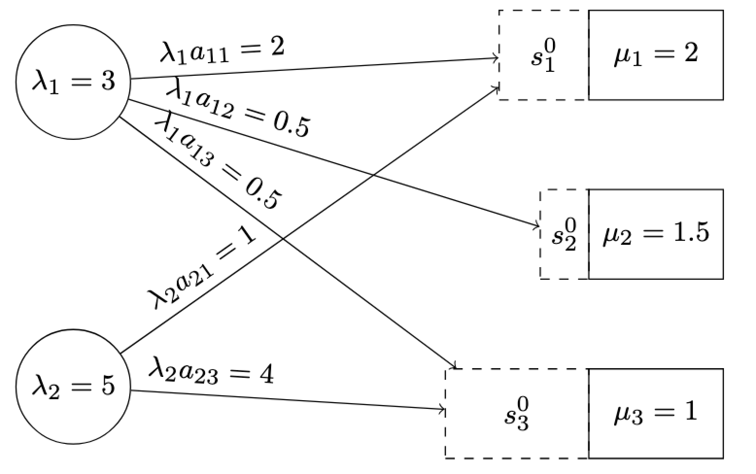
We further assume that each server is initially occupied with a load of jobs. A graphical illustration of the model is provided in Fig. 1. In this example, we consider three servers with initial loads and service rates , , and , respectively. Two players are present, with job lengths and . As shown in the figure, Player 1 has distributed 2 units of its job on Server 1, 0.5 units on Server 2, and the remaining 0.5 units on Server 3. Meanwhile, Player 2 schedules 1 unit of its job on Server 1 and the remainder on Server 3.
Now, let us suppose player has already scheduled portion of its job on server . The amount of time required by server to fully process that portion is given by . In particular, if player schedules an additional infinitesimal portion of its job on server , the delay experienced by that infinitesimal portion to be processed is . Therefore, the wait time for player when scheduling a fraction of its job on server can be calculated as:
Finally, since player schedules different fractions of its job on different servers according to its action , the average wait time of player when taking action can be written as:
| (1) |
Using the same reasoning, given an action profile of all the players, we can define the cost function for player as
| (2) |
Therefore, we obtain a noncooperative static load balancing game , where each player aims to make a decision in order to minimize its own cost function .
2.2 Dynamic Load Balancing Game
The dynamic game setting is the same as the static one, except that the scheduling process evolves over time as more jobs arrive and get processed. More specifically, in the dynamic load balancing game, at each discrete time , we assume that only one player (say player ) receives a job333For instance, if job arrivals follow a continuous random process such as a Poisson process, one may assume that at any time only one of the players receives a new job., and this player must immediately schedule it among the servers. Let us define and as the action of player and the load (state) of server at time , respectively. Moreover, we denote the state of the game at time by , which is the vector of observed loads on each of the servers at time . Now suppose that player receives a new job of length at time and schedules it among the servers according to its action . By following the same derivations as in the static game (Eq. (1)), the instantaneous average wait time for player due to its new job arrival at time equals
| (3) |
After that, the state of server changes according to
| (4) |
where . Finally, the goal for each player is to follow a certain scheduling policy to minimize its overall averaged cumulative cost given by
| (5) |
Assumption 1
In the dynamic load balancing game, we assume that .
We note that Assumption 1 is the stability condition and is crucial in the dynamic setting. Otherwise, one could always consider a worst-case instance where, regardless of any scheduling policy, the length of the waiting jobs in the server queues will grow unboundedly.
3 Main Theoretical Results for the Static Load Balancing Game
In this section, we analyze the static load balancing game and show that it belongs to the class of potential games, for which the best response dynamics are known to converge to a pure Nash equilibrium [43]. We then characterize the best response dynamics in a closed-form as a solution to a convex program. This closed-form solution will be used in the subsequent section to extend our results to the dynamic game setting.
Theorem 1
The static load balancing game is a potential game and admits a pure NE. In particular, the best response dynamics, in which players iteratively and sequentially redistribute their jobs over the servers by best responding to others’ strategies, converge to a pure NE.
Proof 3.2.
We show that the static load balancing game is an exact potential game [43], that is, we show that for any two action profiles and that only differ in the action of player , we have
| (6) |
To that end, let us consider the potential function
For simplicity, let be the effective load on server viewed from the perspective of player , where we note that since do not depend on player ’s action, they must be the same for both action profiles and . We can write
where the last equality is obtained by the expression of the cost function (2) and the definition of . Using an identical argument, we have . Finally, by subtracting this relation from the former one, we get the desired relation (6).
Since the static game is an exact potential game, it admits a pure NE. Moreover, any sequence of best-response updates, in which a player updates its strategy and strictly reduces its cost, will also reduce the potential function. As a result, the best-response dynamics will converge to a local minimum of the potential function, which must be a pure NE.
Remark 3.3.
A more intuitive way to see why serves a potential function is to note that
This in view of [43, Lemma 4.4] suggests that the static load balancing game is a potential game.
Remark 3.4.
One can show that the potential function in the proof of Theorem 1 is strongly convex with respect to each player’s action separately. However, in general, may not be jointly convex with respect to the entire action profile . Otherwise, we would have a unique pure NE.
Next, we proceed to characterize the best response of each player in a closed-form. To that end, let us define to be the relative available processing rate of server that is viewed by player , i.e.,
Then, we can rewrite the cost function (2) as
| (7) |
Given fixed strategies of the other players , a simple calculation shows that the entries of the Hessian matrix of the cost function (7) with respect to are given by
Therefore, the Hessian of with respect to is a diagonal matrix with strictly positive diagonal entries, and hence, it is a positive-definite matrix. This shows that the cost function of each player is strongly convex with respect to its own action.
Now suppose player plays its best-response action to the fixed actions of the other players (including the initial loads on the servers). As in [38], we can write a convex program whose solution gives us the best strategy for player :
| (8) | ||||
| (9) | ||||
| (10) |
Since the objective function is strongly convex with respect to the decision variable , we can use KKT optimality conditions to solve the optimization problem (8) in a closed-form. The result is stated in the following lemma.
Lemma 3.5.
Given player , assume the servers are sorted according to their available processing rates, i.e., . Then, the optimal solution of the convex program (8) is given by
| (11) |
where is the smallest integer index satisfying
Proof 3.6.
Let us consider the Lagrangian function for player , which is given by:
where and are Lagrange multiplies corresponding to the constraints in (8). Since (8) is a convex program, using KKT optimality conditions, we know that is the optimal solution (for a fixed ) if and only if:
Using the first condition, we have:
If , we know that , which results in:
If , we have
Suppose we sort the servers according to their available processing rates such that
Now, a key observation is that a server with a higher available processing rate should naturally have a higher fraction of jobs assigned to it. Under the assumption that the servers are sorted by their available processing rates, the load fractions on the servers also should follow the same ordering, i.e.,
Consequently, there may be cases where slower servers are assigned no jobs. This implies the existence of an index such that
Therefore, suppose player only distributes its job among the servers . We have
Finally, for , we have
where is the smallest index satisfying
In Theorem 1, we established that the best-response dynamics in the static game converge to a pure NE. In fact, using the closed-form characterization of the best responses in Lemma 11, we can prove a stronger result regarding the convergence time of the best-response dynamics to a pure NE in the static game. More specifically, we can show that under a mild assumption on the initial strategies, if each player updates their strategy exactly once using the best-response update rule (11), the game will reach a pure NE. This result is stated formally in the following theorem.
Theorem 3.7.
Suppose in the static load balancing game each player is initially distributing a non-zero portion of its job on each server, i.e., . Then, the action profile obtained when players update their actions exactly once (in any order) using the best-response rule in (11) is a pure NE. In other words, the best-response dynamics converge to a pure NE in iterations.
Proof 3.8.
Please see Appendix A.1 for the proof.
4 Main Theoretical Results for the Dynamic Load Balancing Game
In this section, we consider the dynamic load balancing game and present our main theoretical results. As we saw in Section 3, the static load balancing game admits a pure NE, and iterative best-response dynamics converge to one such NE point. Therefore, a natural question arises: will following the best-response dynamics in the dynamic game also lead to a NE? The main result of this section is to show that this is indeed the case, and to establish a bound on the number of iterations required for the dynamics to converge to a fully balanced distribution of loads across the servers.
Upon arrival of a new job at time to some player with job length :
-
•
Player observes the state at time , computes the available processing rates , and sorts them in an increasing order, where without loss of generality, we may assume
-
•
Player computes its best response at time by solving the convex program , whose solution is given by
where is the smallest index satisfying:
-
•
Player schedules portion of its job on server , and the game proceeds to the next step .
Algorithm 1 describes the best-response dynamics for the dynamic load balancing game. In this algorithm, at each time , the player receiving a job distributes it among the servers according to its best-response strategy relative to the current state. The following lemma establishes a key property of the update rule in Algorithm 1.
Lemma 4.9.
Suppose each player follows Algorithm 1 in the dynamic load balancing game. Then, there exists a finite time after which any player must distribute its job among all the servers, i.e., .
Proof 4.10.
Following Algorithm 1, suppose at an arbitrary time player distributes its job to the set of servers indexed by , while sending nothing to the servers in , i.e.,
| (12) |
where is the smallest index satisfying:
| (13) |
At time , let us define
| (14) |
which in view of (12) implies that
| (15) |
Therefore, according to (4), the states of the servers evolve as
| (16) |
and
| (17) |
where the last inequality is obtained using the update rule of Algorithm 1 as for , we have .
Now, either , in which case by (16) all the servers in become empty at time , or , in which case by (16) and (17), the servers would still have some load remaining on them at time . In either case, using (16) and (17), we have
| (18) |
or equivalently,
| (19) |
This shows that once a player distributes its job among a set of servers, those servers will continue to receive jobs in future iterations simply because the order of those servers in terms of available processing rates remains on the top of the list. More precisely, let us denote the set of servers that receive a job at time by , and suppose another player (say player ) updates at time and wants to distribute its job among the servers. Then, according to Algorithm 1, player would send its job to all the servers in because they all have the highest order in the list (19), and possibly more servers examined in the same order as (19). Therefore, the set of servers receiving a job at time is a superset of those that receive a job at time , and they form a nested sequence of sets over time, i.e.,
| (20) |
Next, we argue that the nested sequence (20) must grow until it eventually includes all the servers, i.e., for some . In particular, using (20), we must have , which means that all the servers must receive a job after time , completing the proof.
To show that the nested sequence (20) must grow, we first note that if a server becomes empty at some time , i.e., , then . Thus, server must receive a job at the next time step , and so by the nested property (20), it must receive a job in all subsequent iterations. Since , it means that in all iterations , server did not receive a new job and was only processing its initial load at rate . Otherwise, server must have previously received a job and thus would be in the set by the nested property (20). Therefore, the load of server at time would be . As a result, server does not belong to for at most iterations, after which its load becomes zero and according to the above discussion, it will receive a job in the next iteration. By repeating this argument for any choice of server , one can see that after at most iterations, we must have .
We are now ready to state the main result of this section.
Theorem 4.11.
If all the players follow Algorithm 1, after
iterations,444We refer to Appendix A.2 for an alternative bound on the number of iterations , which may be better for a certain range of parameters. the state of each server becomes zero (i.e., the system becomes load-balanced). In particular, the strategies of the players converge to the pure NE of the static load balancing game with zero initial loads.
Proof 4.12.
From Lemma 4.9, we know that once a player begins sending jobs to all servers, all subsequent players will continue to do so for the remainder of the time. Consider an arbitrary time , and assume that at time player receives a job and plays its best-response according to Algorithm 1. Since all servers receive jobs at time , we have
Moreover, if player schedules its job at time , then
| (21) |
There are two possible cases:
- •
-
•
If , then , and thus using (21), we have . By repeating this argument inductively, one can see that .
Using the above cases, one can see that if for some , then the value of decreases by at least in the next time step, where . Therefore, after a finite number of iterations
| (23) | ||||
| (24) |
we must have . In particular, for any time , the best-response action for the updating player takes a simple form of
that is, each server receives a fraction of the job proportional to its service rate and the load on each server would become .
Finally, we note that since for , the dynamic load balancing game reduces to the static load balancing game with zero initial loads, i.e., . Since by Theorem 1, the best-response strategy in the static game converges to a pure NE, we obtain that for any and , which is precisely the pure NE of the static game with zero initial loads.
5 Numerical Experiments
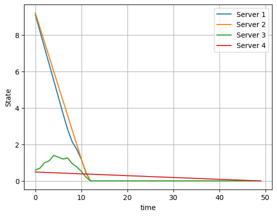
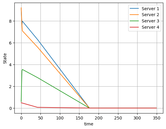
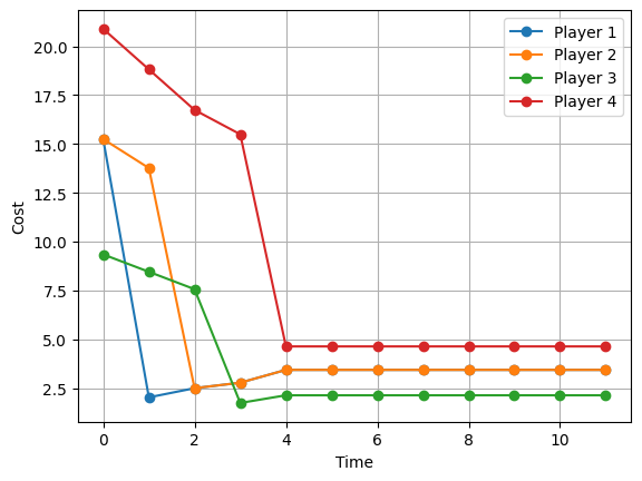
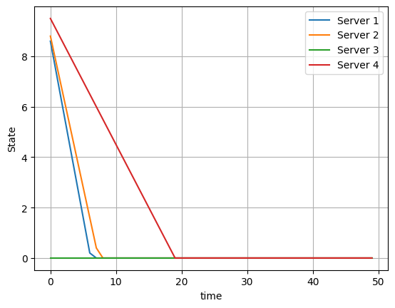
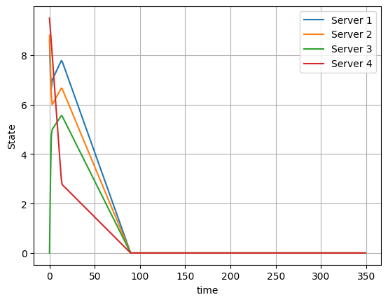
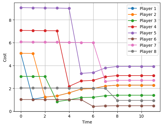
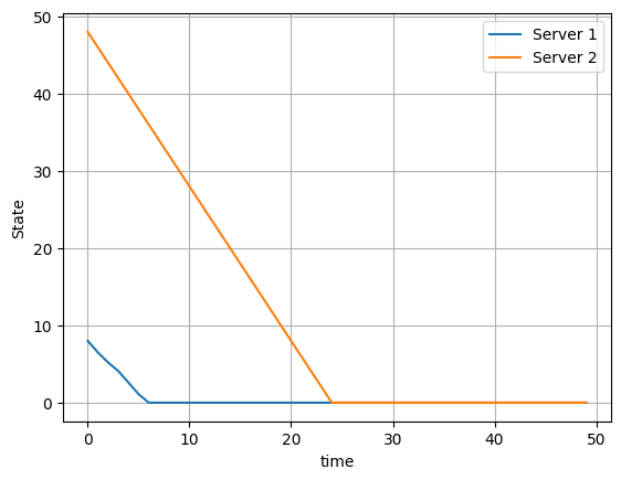
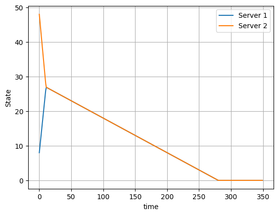
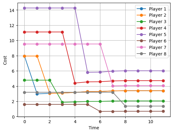
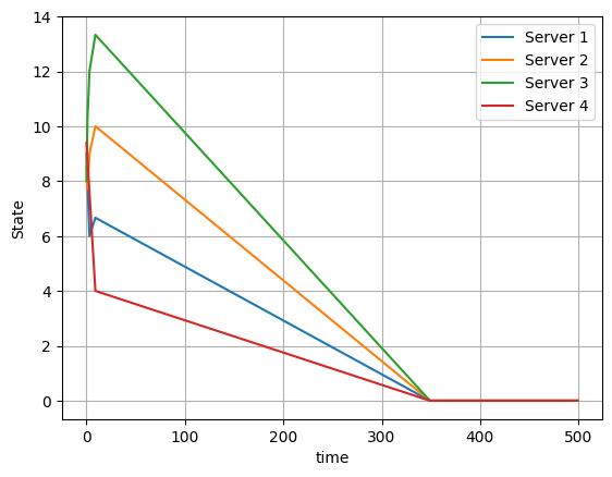
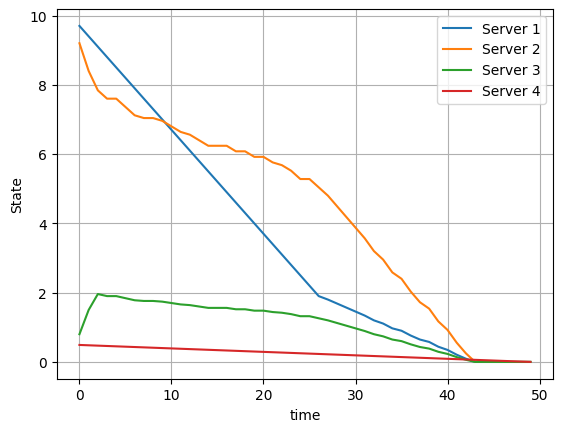
In this section, we present numerical results to evaluate the performance of the best-response dynamics under various settings of the static game, dynamic game, sequential update rule, and simultaneous update rule. In our simulations, we consider three different choice of parameters for the initial state, players’ job lengths, and servers’ service rates, where the parameters for each setting are provided in the captions of the corresponding figures. For instance, in the first row of Fig. 2, we consider a settings with four servers with initial loads and service rates , and a set of four players with job lengths .
First, we simulate the performance of Algorithm 1 for the dynamic load balancing game, where at each time step, a single player is randomly selected to distribute its job across the servers. The results of this experiment are illustrated in Figs. 2(a), 2(d), 2(g), 3(a), and 3(b). As can be seen, after sufficient time has elapsed, all states converge to zero. Once the load on all servers becomes zero, it remains at zero, indicating a stable NE. As illustrated in these figures, the convergence of the dynamics to the zero state appears to be fast and scales polynomially with respect to the game parameters, which also justifies the theoretical performance guarantee provided by Theorem 4.11.
Next, we evaluate an alternative version of Algorithm 1 for the dynamic load balancing game, in which, at each time step, all players simultaneously distribute their jobs. In this case, each player adopts the best-response strategy, considering both the current state of the system and the strategies of other players. The results of this experiment are depicted in Figs. 2(b), 2(e), and 2(h). Interestingly, the results show that the simultaneous update of the players does not hurt the overall performance of the system and the state of the game eventually converges to zero, albeit at a slower convergence rate.
Finally, in Figs. 2(c), 2(f), and 2(i), we evaluate the performance of the sequential best-response dynamics in the static load balancing game, where for all . As can be seen, the action profiles converge to a pure Nash equilibrium (NE) after exactly iterations (one update by each player), which confirms the theoretical convergence rate bound provided in Theorem 3.7.
6 Conclusions
In this work, we develop a game-theoretic framework for load balancing in static and dynamic settings, motivated by practical applications in job scheduling and cyber-physical systems. We demonstrate that the static game formulation is a potential game, which guarantees the existence of a pure Nash equilibrium, with best-response dynamics converging in a finite number of iterations. To account for the carryover effect, we extend our formulation to dynamic settings and show that players employing best-response strategies in each state can achieve a fully load-balanced system, with convergence to the Nash equilibrium of the static game occurring in polynomial time. Our numerical experiments validate the efficiency of the proposed algorithms.
These findings provide a solid foundation for further exploration into more complex load-balancing strategies in distributed systems. One promising direction for future work is to explore scenarios where all players update their strategies and distribute jobs simultaneously in each round of the dynamic game. While our numerical experiments suggest that the dynamic game would still converge to a load-balanced static game, the convergence rate is notably slower. Another interesting direction is to extend our work to stochastic settings, where servers have stochastic processing rates and process the jobs assigned to them with certain probabilities.
References
References
- [1] I. Milchtaich, “Congestion games with player-specific payoff functions,” Games and Economic Behavior, vol. 13, no. 1, pp. 111–124, 1996.
- [2] R. Holzman and N. Law-Yone, “Strong equilibrium in congestion games,” Games and Economic Behavior, vol. 21, no. 1-2, pp. 85–101, 1997.
- [3] S. Shahrampour, A. Rakhlin, and A. Jadbabaie, “Multi-armed bandits in multi-agent networks,” in 2017 IEEE International Conference on Acoustics, Speech and Signal Processing (ICASSP), 2017, pp. 2786–2790.
- [4] J. Vermorel and M. Mohri, “Multi-armed bandit algorithms and empirical evaluation,” in European conference on machine learning, 2005, pp. 437–448.
- [5] J. Gaitonde and É. Tardos, “Stability and learning in strategic queuing systems,” in Proceedings of the 21st ACM Conference on Economics and Computation, 2020, pp. 319–347.
- [6] X. Zhou, F. Wu, J. Tan, K. Srinivasan, and N. Shroff, “Degree of queue imbalance: Overcoming the limitation of heavy-traffic delay optimality in load balancing systems,” Proceedings of the ACM on Measurement and Analysis of Computing Systems, vol. 2, no. 1, pp. 1–41, 2018.
- [7] T. Hellemans and B. Van Houdt, “On the power-of-d-choices with least loaded server selection,” Proceedings of the ACM on Measurement and Analysis of Computing Systems, vol. 2, no. 2, pp. 1–22, 2018.
- [8] I. A. Horváth, Z. Scully, and B. Van Houdt, “Mean field analysis of join-below-threshold load balancing for resource sharing servers,” Proceedings of the ACM on Measurement and Analysis of Computing Systems, vol. 3, no. 3, pp. 1–21, 2019.
- [9] M. Mitzenmacher, “The power of two choices in randomized load balancing,” IEEE Transactions on Parallel and Distributed Systems, vol. 12, no. 10, pp. 1094–1104, 2001.
- [10] H.-C. Lin and C. S. Raghavendra, “A dynamic load-balancing policy with a central job dispatcher (lbc),” IEEE Transactions on Software Engineering, vol. 18, no. 2, p. 148, 1992.
- [11] V. Gupta, M. H. Balter, K. Sigman, and W. Whitt, “Analysis of join-the-shortest-queue routing for web server farms,” Performance Evaluation, vol. 64, no. 9-12, pp. 1062–1081, 2007.
- [12] P. Eschenfeldt and D. Gamarnik, “Join the shortest queue with many servers. the heavy-traffic asymptotics,” Mathematics of Operations Research, vol. 43, no. 3, pp. 867–886, 2018.
- [13] R. D. Foley and D. R. McDonald, “Join the shortest queue: stability and exact asymptotics,” Annals of Applied Probability, pp. 569–607, 2001.
- [14] M. Kogias, G. Prekas, A. Ghosn, J. Fietz, and E. Bugnion, “R2P2: Making RPCs first-class datacenter citizens,” in 2019 USENIX Annual Technical Conference (USENIX ATC 19), 2019, pp. 863–880.
- [15] M. Kogias and E. Bugnion, “Hovercraft: Achieving scalability and fault-tolerance for microsecond-scale datacenter services,” in Proceedings of the Fifteenth European Conference on Computer Systems, 2020, pp. 1–17.
- [16] K. Gardner and C. Stephens, “Smart dispatching in heterogeneous systems,” ACM SIGMETRICS Performance Evaluation Review, vol. 47, no. 2, pp. 12–14, 2019.
- [17] W. Winston, “Optimality of the shortest line discipline,” Journal of applied probability, vol. 14, no. 1, pp. 181–189, 1977.
- [18] Y. Lu, Q. Xie, G. Kliot, A. Geller, J. R. Larus, and A. Greenberg, “Join-idle-queue: A novel load balancing algorithm for dynamically scalable web services,” Performance Evaluation, vol. 68, no. 11, pp. 1056–1071, 2011.
- [19] M. Mitzenmacher, “Analyzing distributed join-idle-queue: A fluid limit approach,” in 2016 54th Annual Allerton Conference on Communication, Control, and Computing (Allerton), 2016, pp. 312–318.
- [20] B. Jennings and R. Stadler, “Resource management in clouds: Survey and research challenges,” Journal of Network and Systems Management, vol. 23, no. 3, pp. 567–619, 2015.
- [21] Q. Xie, X. Dong, Y. Lu, and R. Srikant, “Power of d choices for large-scale bin packing: A loss model,” ACM SIGMETRICS Performance Evaluation Review, vol. 43, no. 1, pp. 321–334, 2015.
- [22] K. Gardner, M. Harchol-Balter, A. Scheller-Wolf, M. Velednitsky, and S. Zbarsky, “Redundancy-d: The power of d choices for redundancy,” Operations Research, vol. 65, no. 4, pp. 1078–1094, 2017.
- [23] K. Ousterhout, P. Wendell, M. Zaharia, and I. Stoica, “Sparrow: distributed, low latency scheduling,” in Proceedings of the twenty-fourth ACM symposium on operating systems principles, 2013, pp. 69–84.
- [24] A. Roy, L. Bindschaedler, J. Malicevic, and W. Zwaenepoel, “Chaos: Scale-out graph processing from secondary storage,” in Proceedings of the 25th Symposium on Operating Systems Principles, 2015, pp. 410–424.
- [25] M. A. U. Nasir, G. D. F. Morales, D. Garcia-Soriano, N. Kourtellis, and M. Serafini, “The power of both choices: Practical load balancing for distributed stream processing engines,” in 2015 IEEE 31st International Conference on Data Engineering, 2015, pp. 137–148.
- [26] H. Zhu, K. Kaffes, Z. Chen, Z. Liu, C. Kozyrakis, I. Stoica, and X. Jin, “RackSched: A Microsecond-Scale scheduler for Rack-Scale computers,” in 14th USENIX Symposium on Operating Systems Design and Implementation (OSDI 20), 2020, pp. 1225–1240.
- [27] H. Kameda, J. Li, C. Kim, and Y. Zhang, Optimal load balancing in distributed computer systems, 2012.
- [28] T. Roughgarden, “Stackelberg scheduling strategies,” in Proceedings of the 33rd Annual ACM Symposium on Theory of Computing, 2001, pp. 104–113.
- [29] J. F. Nash Jr, “The bargaining problem,” Econometrica: Journal of the Econometric Society, pp. 155–162, 1950.
- [30] A. A. Economides, J. A. Silvester et al., “Multi-objective routing in integrated services networks: A game theory approach.” in Infocom, vol. 91, 1991, pp. 1220–1227.
- [31] A. A. Economides and J. A. Silvester, “A game theory approach to cooperative and non-cooperative routing problems,” in SBT/IEEE International Symposium on Telecommunications, 1990, pp. 597–601.
- [32] A. Orda, R. Rom, and N. Shimkin, “Competitive routing in multiuser communication networks,” IEEE/ACM Transactions on Networking, vol. 1, no. 5, pp. 510–521, 1993.
- [33] E. Altman, T. Basar, T. Jiménez, and N. Shimkin, “Routing into two parallel links: Game-theoretic distributed algorithms,” Journal of Parallel and Distributed Computing, vol. 61, no. 9, pp. 1367–1381, 2001.
- [34] Y. A. Korilis, A. A. Lazar, and A. Orda, “Capacity allocation under noncooperative routing,” IEEE Transactions on Automatic Control, vol. 42, no. 3, pp. 309–325, 1997.
- [35] E. Koutsoupias and C. Papadimitriou, “Worst-case equilibria,” in Annual symposium on theoretical aspects of computer science, 1999, pp. 404–413.
- [36] M. Mavronicolas and P. Spirakis, “The price of selfish routing,” in Proceedings of the thirty-third annual ACM Symposium on Theory of Computing, 2001, pp. 510–519.
- [37] T. Roughgarden and É. Tardos, “How bad is selfish routing?” Journal of the ACM (JACM), vol. 49, no. 2, pp. 236–259, 2002.
- [38] D. Grosu and A. T. Chronopoulos, “Noncooperative load balancing in distributed systems,” Journal of parallel and distributed computing, vol. 65, no. 9, pp. 1022–1034, 2005.
- [39] D. Grosu, A. T. Chronopoulos, and M.-Y. Leung, “Load balancing in distributed systems: An approach using cooperative games,” in In Proceedings of the 16th IEEE International Parallel and Distributed Processing Symposium, 2002, pp. 10–pp.
- [40] A. Schaerf, Y. Shoham, and M. Tennenholtz, “Adaptive load balancing: A study in multi-agent learning,” Journal of Artificial Intelligence Research, vol. 2, pp. 475–500, 1994.
- [41] S. Krishnasamy, R. Sen, R. Johari, and S. Shakkottai, “Regret of queueing bandits,” Advances in Neural Information Processing Systems, vol. 29, 2016.
- [42] J. Gaitonde and E. Tardos, “Virtues of patience in strategic queuing systems,” in Proceedings of the 22nd ACM Conference on Economics and Computation, 2021, pp. 520–540.
- [43] D. Monderer and L. S. Shapley, “Potential games,” Games and Economic Behavior, vol. 14, no. 1, pp. 124–143, 1996.
Appendix A Omitted Proofs
A.1 Proof of Theorem 3.7
Proof A.13.
Without loss of generality and by relabeling the players, let us assume that players update their strategies according to their index, i.e., the th updating player is player . Moreover, let us define to be the set of servers that receive a job from player given its action profile at time . First, we show that if players sequentially update their actions according to their best responses, then .
Consider an arbitrary player who wants to update its action at time . Since players have not updated their actions yet, player plays its best response with respect to the action profile . For each server , define
which is the relative available processing rate of server that is viewed by player at time . Thus, player sorts servers in a way that . Now suppose player sends a job to servers indexed in . We therefore have for :
where is the smallest integer index satisfying
| (25) |
Now, it is player ’s turn to update its policy and it calculates the available processing rate for each server. Thus, we have
| (26) |
There are two possible scenarios:
-
•
: This means that player distributes its job among all servers and we now want to check if player does the same thing. In this case we have
Suppose server is the server with highest , so that player sends job to it. Now, we have to check whether player also sends a job to other servers. Take server as an example. Player sends a portion of its job to server only if
(27) which obviously holds because for all , . More generally, for all and , we have
(28) (29) Thus, we conclude that player , or in other words .
-
•
: Suppose player sends job to servers indexed in . Note that can also be an empty set. We now want to see if it sends any job to servers indexed in . Take server as an example. Player sends job to server only if
(30) (31) According to (25), we already know that
(32) Since for all , we conclude that
and therefore player sends a fraction of its job to server at time . Now, to check whether player also sends a job to the rest of the servers in , let us take an arbitrary server . Then, player sends a job to server only if
(33) (34) (35) In other words, we have to check whether
(36) (37) More generally, for any and , we have
(38) (39) which holds because of (32) and the fact that for all . Since is chosen arbitrarily, we can conclude that .
To complete the proof, we note that when player updates its action, it plays its best response with respect to the action profile . Suppose it sends a portion of its job only to servers indexed in . We therefore know that for . Moreover, we know that player distributes its job in a way such that
In other words, player ensures that the normalized load is equal across all servers receiving jobs. Consequently, for all players, the servers to which they allocate jobs have identical normalized loads, which is exactly what players achieve when playing their best-response strategies. As a result, no player has an incentive to change their policy, as this distribution aligns with their best-response strategy. Thus, forms a pure NE of the static game.
A.2 An Alternative Bound for the Convergence Rate of the Dynamic Game
In this appendix, we provide an alternative bound for the convergence rate of Algorithm 1 in the dynamic load-balancing game, which, for certain ranges of game parameters, could be better than the convergence rate given in Theorem 4.11.
As before, the main idea is to analyze how quickly approaches zero. Define and . Similarly, let and . To lower-bound the amount of decrease in , we consider two cases:
-
•
Not all servers are receiving jobs. In this case, the minimum change occurs when all servers, except the slowest one (the server with the lowest processing rate), receive and process jobs completely. For these servers, we have: . Thus, only the slowest server contributes to the change in . Without loss of generality, suppose the index of this server is , i.e., . There are two possible cases:
-
(1)
: In this case we have . This gives the inequality
-
(2)
: In this case we have , thus . Moreover, since server has not received any job at time , according to (13), we have . This gives us
-
(1)
-
•
All servers are receiving jobs, but the state has not yet converged to zero: According to Theorem 4.11, in this case we have
where is the player sending job at time . Therefore, we have
Thus, putting all of the above cases together, we conclude that the number of iterations until convergence is upper-bounded by: