ToMoE: Converting Dense Large Language Models to Mixture-of-Experts through Dynamic Structural Pruning

Abstract

Large Language Models (LLMs) have demonstrated remarkable abilities in tackling a wide range of complex tasks. However, their huge computational and memory costs raise significant challenges in deploying these models on resource-constrained devices or efficiently serving them. Prior approaches have attempted to alleviate these problems by permanently removing less important model structures, yet these methods often result in substantial performance degradation due to the permanent deletion of model parameters. In this work, we tried to mitigate this issue by reducing the number of active parameters without permanently removing them. Specifically, we introduce a differentiable dynamic pruning method that pushes dense models to maintain a fixed number of active parameters by converting their MLP layers into a Mixture of Experts (MoE) architecture. Our method, even without fine-tuning, consistently outperforms previous structural pruning techniques across diverse model families, including Phi-2, LLaMA-2, LLaMA-3, and Qwen-2.5.

1 Introduction

Large Language Models (LLMs) have emerged as powerful tools in artificial intelligence, exhibiting remarkable capacity in natural language understanding and generation. By leveraging advanced neural architectures (Vaswani et al., 2017), and pretraining on vast corpora of text, these models have demonstrated a remarkable ability to perform diverse tasks, ranging from question answering and machine translation to content creation and scientific discovery (Brown, 2020; Kenton & Toutanova, 2019; Raffel et al., 2020). Examples of popular commercial or non-commercial LLMs include ChatGPT (OpenAI, 2022), Claude (Anthropic, 2023), and LLaMA (Touvron et al., 2023a). The core strength of LLMs lies in their ability to capture complicated relationships within the context, enabling them to generalize across tasks with in-context learning (Dong et al., 2022) or minimal fine-tuning (Radford et al., 2019; Kaplan et al., 2020).

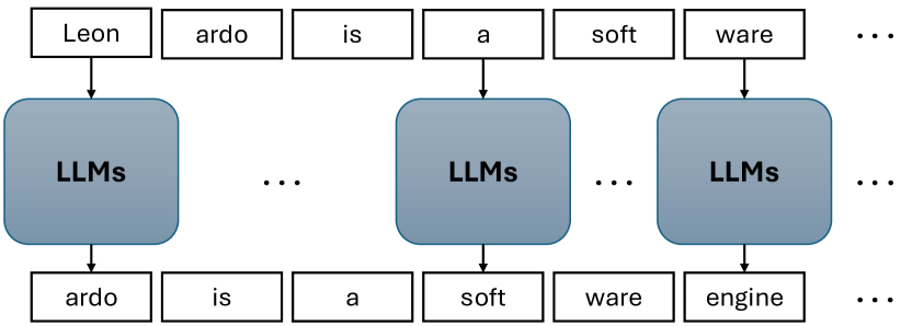
(a)

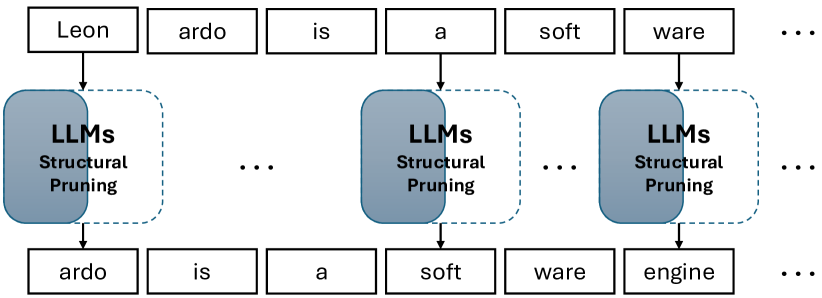
(b)

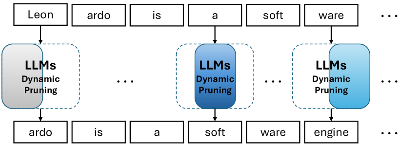
(c)

Figure 1: (a): The original LLM uses all parameters to process all the input text. (b): The static pruning for LLMs permanently removes model parameters, and the rest of the parameters are used to process all the input text. Our approach (c): LLMs with dynamic pruning use different sub-networks to process different tokens. We incorporate MoE to achieve a fixed expected budget in inference.

Although LLMs demonstrate remarkable potential, their huge model size often limits their usability on devices with limited resources. As a result, considerable efforts (Ma et al., 2023; Ashkboos et al., 2024; Frantar et al., 2022) are focused on minimizing the computational and memory costs of these models. Structural pruning (Ma et al., 2023) has emerged as a promising solution to this challenge because, unlike unstructured pruning, it achieves compression without the need for specialized implementations. However, the problem with structural pruning methods is that they will substantially reduce the model capacity resulting in an obvious performance gap compared to the dense model. The fine-tuning cost to even partially recover this gap is tremendous. To achieve a better trade-off between the number of parameters and performance, sparse Mixture of Experts (MoE) models (Shazeer et al., 2017; Lepikhin et al., 2021b) are designed to activate only a subset of the model’s parameters, corresponding to the selected experts. Recently proposed MoE models, such as DeepseekMoE (Dai et al., 2024), demonstrated that they can match the performance of dense models with a similar total parameter count while using a small number of active parameters. Following this lead, we propose that transforming dense models into MoE models could offer a promising approach to bridging the performance gap left by structural pruning methods. Unlike prior efforts to construct MoE models from dense models (Zhu et al., 2024), our findings reveal that MoEs inherently exist within dense models and can be uncovered without updating model weights (continue pretraining). Specifically, we show that these experts can be identified through dynamic structural pruning. These results represent a novel contribution that has not been demonstrated in previous studies.

The core idea of MoE models is conditional computation, where experts are dynamically selected based on input tokens. This concept aligns closely with dynamic pruning methods (Gao et al., 2019), which make pruning decisions given input features. Leveraging this connection, we propose to construct MoE models from dense models by using dynamic structural pruning. Specifically, for Multi-Head self-Attention (MHA) layers, we apply top-K routing and static pruning for compression, while for MLP layers, we transform them into MoE layers using top-1 expert routing. The routing mechanism learned for dynamic structural pruning can be directly applied to serve as the routing module for MoE layers. With differentiable discrete operations, the MoE conversion process can be formulated as a differentiable dynamic pruning problem. With this formulation, we can efficiently convert a dense model to an MoE model at a cost similar to or lower than regular structural pruning methods. The comparison between our method, static pruning, and the original LLM is shown in Fig. 1. The contributions of this work can be summarized as follows:

• Dense-to-MoE Conversion Through Dynamic Pruning: We introduce a novel approach to convert dense models into MoE models through dynamic pruning. Specifically, we implement top-k routing and static pruning for MHA layers along the head dimension and top-1 routing for MLP layers across the learned experts. This formulation ensures sparse and efficient computation while retaining model capacity.

• Joint Optimized Training for Routing and Experts: The proposed method involves jointly optimizing routing modules and expert configurations by solving a regularized optimization problem. Our approach leverages differentiable operations to enable efficient and flexible MoE constructions.

• Consistent Performance Improvements Across Tasks and Models: Our method consistently outperforms state-of-the-art structural pruning techniques on various tasks even without fine-tuning the model weights. This performance improvement is demonstrated across widely used public models such as Phi-2, LLaMA-2, LLaMA-3, and Qwen-2.5.

2 Related Works

Pruning: Structural pruning (Li et al., 2017; Kurtic et al., 2022; Ma et al., 2023) is an attractive technique for real-world deployments since it removes redundant parameters to reduce model size without requiring specialized implementations. Structural pruning methods fall into two main categories: static pruning (Anwar et al., 2017; Molchanov et al., 2019; Fang et al., 2023) and dynamic pruning (Gao et al., 2019; Chen et al., 2020; Anagnostidis et al., 2023; Dong et al., 2024a). Static pruning removes parameters based on input-agnostic importance metrics. For example, LLM-Pruner (Ma et al., 2023) eliminates non-essential coupled structures using gradient-based criteria. The problem with structural pruning is that it often creates a noticeable performance gap relative to dense models (Ma et al., 2023; Ashkboos et al., 2024). In contrast, dynamic pruning removes weights based on input-dependant metrics. Early attempts for dynamic pruning (Gao et al., 2019; Chen et al., 2020) focus on Convolutional Neural Networks, where channels are selectively activated for input samples. Recent works, such as D-LLM (Wang et al., 2024), incorporate the concept of conditional computation into LLMs by selectively skipping layers based on input tokens. The problem with dynamic pruning methods is that they do not have a fixed budget given different inputs, which creates problems when serving LLMs in a mini-batch setting or in the prefilling stage. Our method, on the other hand, converts the dense LLM to a sparse MoE model with fix per-token budget.

MoE: Sparse Mixture-of-Experts (MoE) models improve upon pure structural pruning by maintaining or even enhancing model capacity without a proportional increase in computational cost. For instance, Sparsely-Gated MoE (Shazeer et al., 2017) employs a trainable gating network to select a small subset of experts for each input, enabling the model to scale to thousands of experts efficiently (Lepikhin et al., 2021b). More recent methods like DeepSeekMoE (Dai et al., 2024) further address expert specialization, matching dense-model performance with a similar number of activated parameters. LLAMA-MoE (Zhu et al., 2024) takes a pre-trained dense LLM, splits large feed-forward layers into multiple experts, and then dynamically routes tokens to these experts via a gating network with significant additional training. Unlike LLaMA-MoE, which treats expert construction and learning routing gates (with 200B training tokens) as distinct processes, our method integrates expert construction directly into the pruning stage, eliminating the need for separate training steps.

3 ToMoE

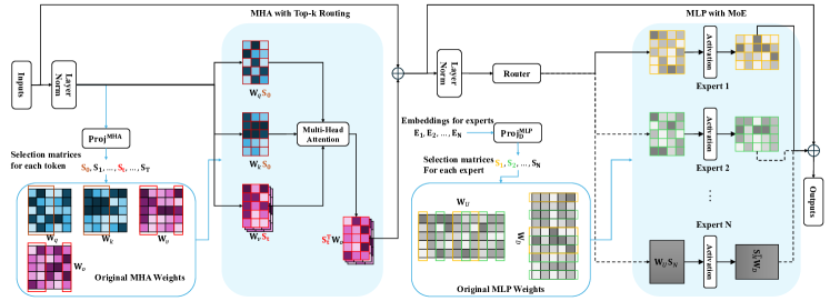
Figure 2: ToMoE uses top-1 routing for MLP layers, and static and dynamic pruning along the head dimension for MHA layers.

Most recent LLMs, like GPT (Radford et al., 2018), LLaMA (Touvron et al., 2023a), etc., adapt decoder-only architectures and thus our method focuses on decoder-only architectures. A typical decoder block consists of Multi-Head Attention (MHA) and Multi-Layer Perceptron (MLP) layers. For clarity, we let $T$, $d$, $d_{\text{mid}}$, and $H$ denote the sequence length, hidden dimension, MLP middle layer dimension, and the number of attention heads, respectively.

To reduce the computational costs of the decoder-only architecture, we propose to convert the original model into MoE models. For MHA layers, we utilize top-k routing and static pruning along the head dimension $\frac{d}{H}$. Top-k routing and static pruning for MHA layers ensure that, during prefilling, all tokens maintain the same head dimension, enabling parallel processing. For MLP layers, our approach transforms them into MoE layers along the MLP middle dimension $d_{\text{mid}}$ and employs top-1 routing. A key distinction between our method and previous dynamic pruning approaches is that the converted model maintains consistent computational costs for all inputs. This property could be crucial for efficient model serving.

3.1 Expert Embeddings

Inspired by the recent success of using hypernetworks (Ha et al., 2016; Ganjdanesh et al., 2024; Gao et al., 2024) to generate pruning decisions, we adopt a hypernetwork to generate expert embeddings:

$$~\mathbf{E}_{\text{all}}=\text{HN(z)}$$ (1)

where the $z$ is the input to the hypernetwork drawn from a random distribution, and $\mathbf{E}_{\text{all}}=[\mathbf{E}_{1},\cdots,\mathbf{E}_{l},\cdots,\mathbf{E}_{L}]$ contains embeddings for all layers and $\mathbf{E}_{l}\in\Re^{N\times d_{e}}$, where $N$ is the number of experts and $d_{e}$ is the expert embedding dimension. The purpose of having the hypernetwork to generate $\mathbf{E}_{\text{all}}$ is to introduce inter-layer dependencies across different layers and operations. This design has been shown to accelerate the learning process in practice (Gao et al., 2024). More details are given in the Appendix A.

3.2 Expert Construction

In this section, we will talk about how to construct experts from MLP layers. In a decoder layer, the formulation of MLP is: $f_{\text{MLP}}(\mathbf{X})=\sigma(\mathbf{X}\mathbf{W}_{G})\odot(\mathbf{X}\mathbf{W}_{U})\mathbf{W}_{D}$, where matrices $\mathbf{W}_{U}\in\Re^{d\times d_{\text{mid}}}$, $\mathbf{W}_{G}\in\Re^{d\times d_{\text{mid}}}$ and $\mathbf{W}_{D}\in\Re^{d_{\text{mid}}\times d}$ denote up, gated, down projection matrices, $\sigma$ denotes nonlinear activation functions and $\odot$ denotes the Hadamard product (element-wise product).

Assume we want to have $N$ experts, under the setting of structural pruning, each expert can be represented by:

$$~f_{\text{MLP}}^{i}(\mathbf{X})=\sigma(\mathbf{X}\mathbf{W}_{G}\mathbf{S}_{i})\odot(\mathbf{X}\mathbf{W}_{U}\mathbf{S}_{i})\mathbf{S}_{i}^{\top}\mathbf{W}_{D}$$ (2)

where $i=1,\ldots,N$, $\mathbf{S}_{i}=\text{Diag}(\mathbf{s}_{i})$ ($\mathbf{s}_{i}\in\Re^{d_{\text{mid}}}$, $\mathbf{S}_{i}\in\Re^{d_{\text{mid}}\times d_{\text{mid}}}$), is a diagonal matrix with 0 or 1 and it is used to select a subset of weight vectors for the $i$th expert. After we have the formulation for each expert, we need to learn the configurations of each expert as shown below:

$$~\mathbf{s}={\text{ST-GS}}(\text{Proj}_{\text{D}}^{\text{\tiny MLP}}(\mathbf{G}\mathbf{E})),\ \mathbf{G}={\text{ST-G}}(\text{Router}(\mathbf{X}))$$ (3)

where $\mathbf{G}\in\Re^{T\times N}$ is the output of the router module, $\mathbf{E}$ ($l$ is omitted for clarity) is the expert embeddings, $\text{Proj}_{\text{D}}^{\text{\tiny MLP}}:\Re^{d_{e}}\to\Re^{d_{\text{mid}}}$ is a projection module to project the latent embedding to the MLP middle dimension, and ST-GS and ST-G are Straight-Through Gumbel-Sigmoid and Gumbel-Softmax functions respectively (Jang et al., 2016). Under this setting, $\mathbf{s}_{i}$ will contain retained positions (represented by $1$) for the $i$th expert and $\mathbf{G}$ contains one-hot routing decisions for different tokens in $\mathbf{X}$.

3.3 MHA top-K Routing

A MHA layer can be represented as: $f_{\text{MHA}}(\mathbf{X})=\sum_{i=1}^{H}\sigma_{s}\left({e}(\mathbf{X}\mathbf{W}_{Q,i}){e}^{\top}(\mathbf{X}\mathbf{W}_{K,i})\right)\mathbf{X}\mathbf{W}_{V,i}{\mathbf{W}_{O,i}}$, where $\mathbf{W}_{Q,i},\mathbf{W}_{K,i},\mathbf{W}_{V,i}\in\Re^{d\times\frac{d}{H}},\mathbf{W}_{O,i}\in\Re^{\frac{d}{H}\times d}$ are the query, key, value, and output matrices for each attention head, and $\mathbf{X}\in\Re^{T\times d}$ is the input hidden states. ${e}$ and $\sigma$ denote positional embedding and the softmax function.

For MHA layers, we perform two kinds of pruning: dynamic top-K pruning and static pruning, both along the head dimension. More specifically, we can also insert selection matrices like MLP layers:

$$~\begin{split}f_{\text{MHA}}(\mathbf{X}_{t})&=\sum_{i=1}^{H}[\sigma_{s}\left({e}(\mathbf{X}_{t}\mathbf{W}_{Q,i})\mathbf{S}_{0}\mathbf{S}_{0}^{\top}{e}^{\top}(\mathbf{X}_{t}\mathbf{W}_{K,i})\right)\\ &\mathbf{X}_{t}\mathbf{W}_{V,i}\mathbf{S}_{t}]\mathbf{S}_{t}{\mathbf{W}_{O,i}}\end{split}\vskip-5.0pt$$ (4)

where $\mathbf{S}_{0}\in\Re^{\frac{d}{H}\times\frac{d}{H}}$ is the shared selection matrix for static pruning of query and key matrices and $\mathbf{S}_{t}\in\Re^{\frac{d}{H}\times\frac{d}{H}}$ is the selection matrix for the value and output matrices of the $t$th token. We apply the same selection matrix across all heads, ensuring that all heads have the same head dimensions at the inference time. To generate the selection matrix, we calculate its diagonal vector $\mathbf{s}_{t}$ as:

$$~\mathbf{s}_{t}={\text{ST-GS}}(\text{Proj}_{\text{D}}^{\text{\tiny MHA}}(\text{Proj}_{\text{E}}^{\text{\tiny MHA}}(\mathbf{X}_{t})+\frac{1}{N}\mathbf{1}^{\top}\mathbf{E})),$$ (5)

where $\mathbf{1}\in\Re^{N\times 1}$ is an all one vector, $\frac{1}{N}\mathbf{1}^{\top}\mathbf{E}$ represents the average expert embedding of size $d_{e}$, $\text{Proj}_{\text{D}}^{\text{\tiny MHA}}:\Re^{d_{e}}\to\Re^{\frac{d}{H}}$ is a project module to project the latent embedding to the head dimension and $\text{Proj}_{\text{E}}^{\text{\tiny MHA}}:\Re^{d}\to\Re^{d_{e}}$ is also a project module to project input tokens to the space of expert embeddings, and ST-GS is defined in Sec. 3.2. When $t=0$, we let $\mathbf{X}=0$, and $\mathbf{s}_{0}={\text{ST-GS}}(\text{Proj}_{\text{D}}^{\text{\tiny MHA}}(\frac{1}{N}\mathbf{1}^{\top}\mathbf{E}))$ since it is input independent.

During training, the number of ones in $\mathbf{s}$ can vary freely. After training is complete, we compute $K=\text{round}(\frac{1}{T}\sum_{t=1}^{T}\sum_{i=1}^{\frac{d}{H}}\mathbf{s}_{t,i})$ for a subset of tokens and use it for top-K routing during inference. Note that the $k$ in top-k for $\mathbf{s}_{0}$ and $\mathbf{s}_{t}$ ($t\geq 1$) can be different, allowing for larger flexibility. Also, note that $\mathbf{s}_{0}$ needs to have specific structures to comply with the position embedding $e(\cdot)$, and more details are given in the Appendix A.2.

Table 1: Perplexity comparisons of structured pruning methods and ToMoE for LLaMA-2 7B and 13B models on WikiText-2.

Method	LLaMA-2 7B (ppl: 5.12 $\downarrow$)			LLaMA-2 13B (ppl: 4.57 $\downarrow$)
	70%	60%	50%	70%	60%	50%
LLM-Pruner (Ma et al., 2023)	13.56	17.90	31.05	12.19	19.56	32.20
LLM Surgeon (van der Ouderaa et al., 2024)	7.83	10.39	15.38	6.21	7.25	9.43
ShortGPT (Men et al., 2024)	33.21	71.04	268.11	30.48	48.83	187.23
SLEB (Song et al., 2024)	11.23	29.10	103.38	8.24	11.76	27.67
SliceGPT (Ashkboos et al., 2024)	10.47	15.19	24.82	8.68	12.56	20.57
ModeGPT (Lin et al., 2024)	7.51	8.41	11.88	6.10	6.95	8.95
DISP-LLM (Gao et al., 2024)	6.85	8.11	9.84	5.77	6.59	7.11
ToMoE (ours)	6.41	7.17	8.36	5.54	6.06	6.78

3.4 Regularizations for MoE Constructions

In Sec. 3.2 and Sec. 3.3, we briefly introduced the design space for constructing MoE models using dynamic structural pruning. In this subsection, we will introduce regularizations tailored to the needs of MoE models.

Union of Experts Regularization. An ideal sparse MoE model converted from a dense model should maximize parameter utilization, which means that the total number of parameters in the MoE model should closely approximate the dense model. To add this regularization to our learning process, we push the union of experts to be closer to the original model. More specifically, we use MHA layers as an example:

$$~\mathbf{u}=\bigcup_{i=1}^{T}\mathbf{s}_{i}=1-\prod_{i=1}^{T}(1-\mathbf{s}_{i}),$$ (6)

where $\bigcup$ is the union operator, and $\mathbf{u}$ is the union of all kept positions for each token. For MLP layers, it can be calculated similarly. We than push $\frac{\sum\mathbf{u}}{|\mathbf{u}|}$ ($|\mathbf{u}|$ represents the size of $\mathbf{u}$) to 1:

$$~\mathcal{R}_{\text{U}}=\frac{1}{L}\sum_{l=1}^{L}f(\frac{\sum\mathbf{u}_{l}}{|\mathbf{u}_{l}|},1),$$ (7)

where $f(\cdot,\cdot)$ can be any regression loss functions, and we will choose $f$ later.

Parameter Regularization. For a sparse MoE model, we also need to control the number of active parameters and the number of active parameters should be fixed. To achieve this goal, we can directly penalize the maximum width from different layers. We choose the maximum width over experts instead of the mean, median, or other alternatives because the maximum provides precise control over the upper bound of the maximum number of active parameters.

Let the width of a layer be denoted as $d_{l}^{*}$, $*\in\{\text{MLP},\text{MHA}\}$. For MLP layers, it can be calculated by $d_{l}^{\text{ MLP}}=\max(\mathbf{s}\mathbf{1}_{d_{\text{mid}}})$, where $\mathbf{1}_{d_{\text{mid}}}\in\Re^{d_{\text{mid}}\times 1}$ is an all one vector of size $d_{\text{mid}}$. $\mathbf{s}\mathbf{1}_{\text{mid}}$ produces the width of all experts, and $d_{l}^{\text{ MLP}}$ represents the maximum width across all experts. The width of MHA layers can be calculated similarly. Based on $d_{l}^{*}$, we can calculate the number of active parameters in the model and we denote it as $\text{T}(\mathbf{d_{\text{MoE}}})$, where $\mathbf{d_{\text{MoE}}}=[d_{1}^{*},\cdots,d_{L}^{*}]$. To push the number of activate parameters to a predefined rate $p$, we have:

$$~\mathcal{R}_{\text{P}}=f(\text{T}(\mathbf{d_{\text{MoE}}}),p\text{T}_{\text{total}}),$$ (8)

where $\text{T}_{\text{total}}$ is the total number of parameters, and $p\in(0,1]$ represents the ratios of the active parameters. For $f$ in Eq. 8 and Eq. 7, we use the following function $f$:

$$f(x,y)=\log(\max(x,y)/\min(x,y))$$

Load Balancing Regularization. When we try to find the configurations of experts, we also apply the load balancing regularization to encourage a balanced load across experts (Lepikhin et al., 2021a; Fedus et al., 2022). We follow the load balancing loss from the Switch Transformer (Fedus et al., 2022):

$$~\mathcal{R}_{\text{L}}=N\sum_{i=1}^{N}F_{i}P_{i},$$ (9)

here, $F_{i}=\frac{1}{T}\sum_{t=1}^{T}\mathbbm{1}(\mathbf{G}_{t,i}=1)$, where $\mathbbm{1}(\cdot)$ is an indicator function and that returns $1$ if the condition is true, and $0$ otherwise. $F_{i}$ represents the fraction of tokens assigned to the $i$-th expert. $P_{i}=\frac{1}{T}\sum\sigma_{s}({G}_{t,i})$, where ${G}=\text{Router}(\mathbf{X})$ is the router output before ST-G, and $\sigma_{s}$ is the softmax function again. $P_{i}$ is the fraction of the router probability allocated for the $i$-th expert. $\mathcal{R}_{\text{L}}$ will encourages uniform routing across different experts as shown in (Fedus et al., 2022). The combination of Eq. 8 and Eq. 9 creates an interesting phenomenon where they encourage uniform allocation of width among experts.

Table 2: Comparisons with semi-structured pruning on LLaMA-2.

Method	Structure	50% (7B)	50% (13B)
SparseGPT (2:4)	Semi-structured	10.17	8.32
Wanda (2:4)	Semi-structured	11.02	8.27
Pruner-Zero (2:4)	Semi-structured	10.52	7.41
ToMoE (ours)	Structured	8.36	6.78

3.5 Learning to Construct MoEs

Based on the aforementioned techniques, we can construct MoEs from the dense LLMs by training router parameters, projection parameters, and hypernetwork parameters. At the same time, we freeze all the parameters in the original model. Doing so allows us to quickly construct an effective MoE model with a resource budget comparable to structural pruning. The overall framework of our method is shown in Fig. 2. The overall training objective function can be formulated as:

$$~\min_{\Theta}\ \mathcal{L}(f^{\prime}(x;\mathbf{E}_{\text{all}}),f(x))+\alpha\mathcal{R}_{\mathbf{P}}+\beta\mathcal{R}_{\mathbf{U}}+\gamma\mathcal{R}_{\mathbf{L}},$$ (10)

where $\Theta=[\Theta_{\text{HN}},\Theta_{\text{Router}},\Theta_{\text{Proj-MHA}},\Theta_{\text{Proj-MLP}}]$, $\Theta_{\text{HN}}$ is trainable parameters for the hypernetwork in Eq. 1, $\Theta_{\text{Router}}$ and $\Theta_{\text{Proj-MLP}}$ are trainable parameters for the Router and the project module in Eq. 3, $\Theta_{\text{Proj-MHA}}$ is the trainable parameters of the projection modules given in Eq. 5, $\mathcal{R}_{\mathbf{P}}$, $\mathcal{R}_{\mathbf{U}}$, and $\mathcal{R}_{\mathbf{L}}$ are regularization terms defined in Sec. 3.4, and $\alpha$, $\beta$ and $\gamma$ are hyperparameters to control the strength of these regularization terms. We use $f$ to represent the original dense model and use $f^{\prime}$ as the model equipped with our designed modules for MoE construction. Under this setting, we use $\mathcal{L}(\cdot,\cdot)$ to calculate the KL divergence between the logits of $f$ and $f^{\prime}$ and use it as the guidance to preserve the capacity of the dense model (Hinton et al., 2015). We also found that only using the KL divergence leads to the best performance, and this observation complies with the experimental setup in (Muralidharan et al., 2024). Also, note that we perform in-place knowledge distillation since the original model weights are frozen. Thus the knowledge distillation process does not introduce overheads in terms of GPU memory.

After learning how to construct the MoE, we prune the MLP layer to $N$ experts with shared weights. After pruning the MLP layer, we save $\frac{1}{N}\mathbf{1}^{\top}\mathbf{E}$ for MHA layers as the bias of the $\text{Proj}_{\text{E}}^{\text{\tiny MHA}}$, and we drop $\text{Proj}_{\text{D}}^{\text{\tiny MLP}}$ and convert Eq. 5 into a Top-k routing function as well as use $s_{0}$ for pruning $\mathbf{W}_{Q}$ and $\mathbf{W}_{K}$. Our construction also enables converting the MoE back into a pseudo-MoE model. The MoE model and the pseudo-MoE model are equivalent, and more details are given in the Appendix B.3.

Table 3: Zero-shot task performance of compressed LLaMA-2 7B, LLaMA-3 8B, Qwen-2.5 7B.

Model	Active Parameters	Method	ARC-e	ARC-c	PIQA	WinoG.	HellaS.	Average
			acc-norm	acc-norm	acc-norm	acc	acc-norm
LLaMA-2 7B	100%	Dense	74.58	46.25	79.11	69.06	75.99	69.00
	70%	ShortGPT (Men et al., 2024)	48.65	32.85	64.31	64.33	56.13	53.25
		SliceGPT (Ashkboos et al., 2024)	58.88	33.36	68.55	58.01	49.86	53.73
		LLM Surgeon (van der Ouderaa et al., 2024)	63.09	36.69	73.56	61.09	60.72	59.03
		DISP-LLM  (Gao et al., 2024)	59.81	33.19	71.82	62.27	63.43	58.10
		DISP-LLM Alpaca (Gao et al., 2024)	60.10	37.03	73.72	63.93	62.87	59.53
		ModeGPT (Lin et al., 2024)	63.26	38.73	70.40	67.32	63.26	60.78
		ModeGPT-Alpaca (Lin et al., 2024)	65.49	39.16	73.34	66.22	65.90	62.02
	60%	ShortGPT (Men et al., 2024)	41.16	29.94	60.12	60.46	43.67	47.07
		SliceGPT (Ashkboos et al., 2024)	36.49	24.57	54.90	53.43	34.80	40.84
		LLM Surgeon (van der Ouderaa et al., 2024)	52.31	30.29	69.26	54.38	48.04	50.86
		ModeGPT (Lin et al., 2024)	49.45	30.03	64.96	61.96	53.01	51.88
		ModeGPT-Alpaca (Lin et al., 2024)	59.76	34.73	70.35	64.40	58.63	57.58
		ToMoE (Ours)	63.64	38.74	72.85	62.51	65.84	60.72
	50%	LLM Surgeon  (van der Ouderaa et al., 2024)	44.91	26.28	64.36	52.57	40.29	45.68
		DISP-LLM  (Gao et al., 2024)	43.06	25.85	63.93	54.54	63.43	46.72
		DISP-LLM Alpaca (Gao et al., 2024)	51.14	30.20	68.34	56.20	49.35	51.05
		ToMoE (Ours)	56.65	33.87	71.00	58.56	60.26	56.07
LLaMA-3 8B	100%	Dense	77.69	53.58	80.63	72.69	79.16	72.75
	75%	ShortGPT-Alpaca (Men et al., 2024)	38.13	31.40	60.94	54.22	31.52	43.24
		SliceGPT-Alpaca (Ashkboos et al., 2024)	44.44	29.27	57.56	58.48	41.08	46.17
		ModeGPT-Alpaca (Lin et al., 2024)	67.05	41.13	75.52	69.61	66.49	63.96
	70%	ToMoE (Ours)	71.55	44.71	76.28	68.98	71.84	66.67
	60%	ToMoE (Ours)	65.87	41.64	73.61	63.30	66.42	62.17
Qwen-2.5 7B	100%	Dense	79.42	50.17	79.54	71.35	78.36	71.77
	50%	DISP-LLM Alpaca (Gao et al., 2024)	55.35	34.22	70.29	53.59	55.00	53.69
		ToMoE N=8 (Ours)	61.83	36.77	71.82	57.70	59.55	57.53
		ToMoE N=16 (Ours)	64.81	41.72	73.45	58.48	61.06	59.90
		ToMoE N=24 (Ours)	64.69	39.85	72.96	58.56	63.21	59.85
	40%	DISP-LLM Alpaca (Gao et al., 2024)	52.65	27.99	65.94	53.43	44.11	48.82
		ToMoE N=8 (Ours)	53.80	32.59	69.59	55.49	52.98	52.89
		ToMoE N=16 (Ours)	53.87	33.70	71.98	54.38	55.65	53.92
		ToMoE N=24 (Ours)	55.43	32.85	69.86	57.85	54.62	54.12

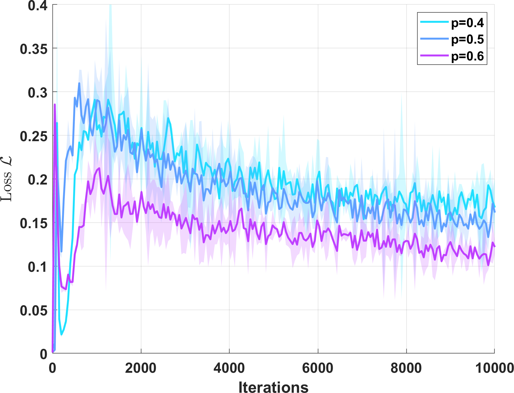
(a)

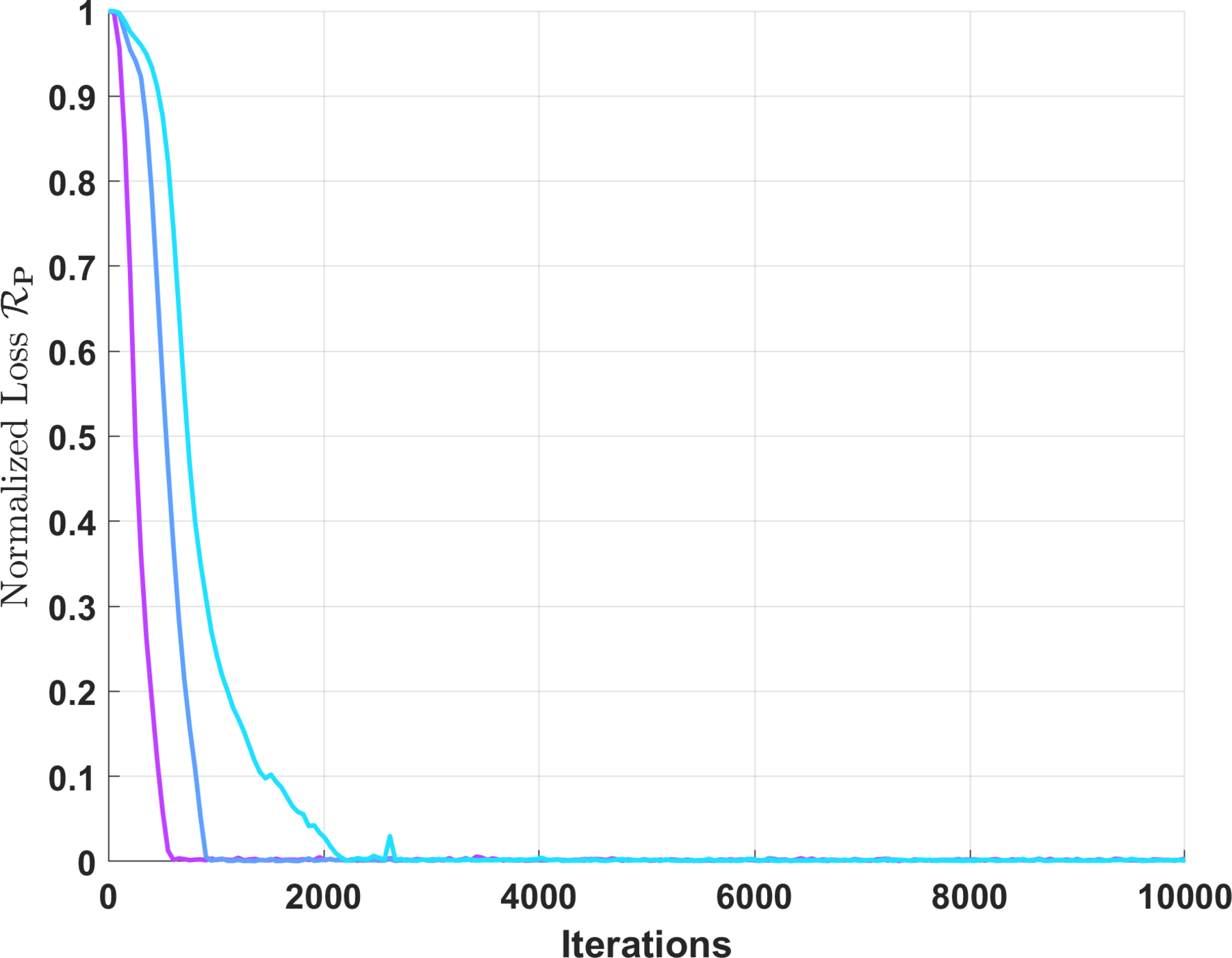
(b)

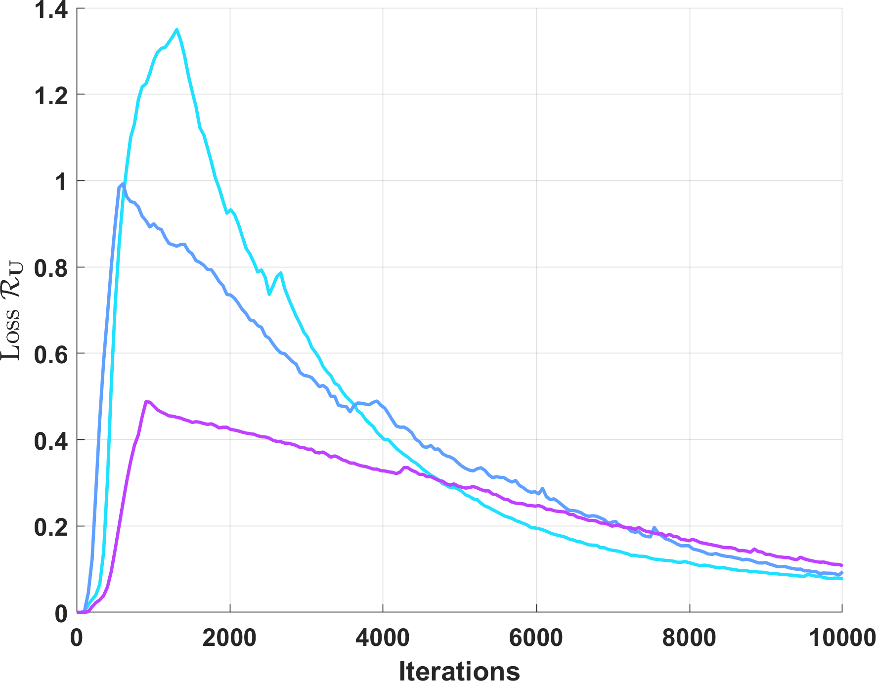
(c)

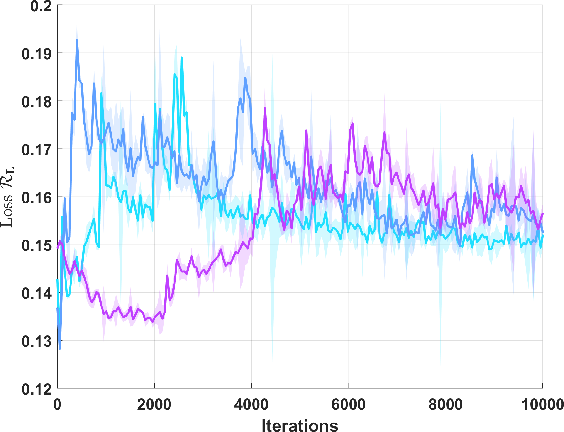
(d)

Figure 3: The training dynamics give different ratios $p$ of active parameters on the Qwen-2.5 7B model.

4 Experiments

4.1 Settings

Models. We evaluate our ToMoE method using several LLMs with decoder blocks. Specifically, we choose the following models: LLaMA-2 (Touvron et al., 2023b): LLaMA-2 7B and LLaMA-2 13B; LLaMA-3 8B (Dubey et al., 2024); Phi-2 (Javaheripi et al., 2023) (shown in Appendix D); Qwen-2.5 (Yang et al., 2024): Qwen-2.5 7B and Qwen-2.5 14B.

Implementations. We implemented ToMoE using Pytorch (Paszke et al., 2019) and Hugging Face transformer library (Wolf et al., 2020). We freeze the model weights when training the modules with learnable parameters $\Theta$ in Eq. in Obj. 10. We use the AdamW (Loshchilov & Hutter, 2019) optimizer to optimize $\Theta$. $\Theta$ is trained for 10,000 iterations for all models. For all experiments, we set $\alpha=16$, $\beta=2.0$, and $\gamma=1.0$, where $\alpha$, $\beta$, and $\gamma$ are defined in Obj. 10. Without specific descriptions, the number of experts for ToMoE is $8$ across all settings. Depending on the size of the base model, we use 1 to 4 NVIDIA A100 GPUs to train $\Theta$. More implementation details can be found in the Appendix C.

Datasets. We provide two training settings for all modules with learnable parameters $\Theta$: (1) using WikiText, and (2) using a mixed dataset comprising WikiText, Alpaca, and Code-Alpaca (mixing ratio: 1:1:1). Based on our understanding, ToMoE benefits from a diverse mixture of datasets to effectively construct experts. Following previous methods (Ashkboos et al., 2024; Gao et al., 2024), we evaluate our method and other methods on five well-known zero-shot tasks: PIQA (Bisk et al., 2020); WinoGrande (Sakaguchi et al., 2021); HellaSwag (Zellers et al., 2019); ARC-e and ARC-c (Clark et al., 2018). We use llm-eval-harness (Gao et al., 2021) to evaluate the compressed models.

Baselines. We compare ToMoE across baselines from structural pruning like LLM-Pruner (Ma et al., 2023), SliceGPT (Ashkboos et al., 2024), ShortGPT (Men et al., 2024), SLEB (Song et al., 2024), LLMSurgeon (van der Ouderaa et al., 2024), ModeGPT (Lin et al., 2024), and DISP-LLM (Gao et al., 2024). We also include semi-structure pruning baselines like SparseGPT (Frantar & Alistarh, 2023), Wanda (Sun et al., 2024), and Pruner-Zero (Dong et al., 2024b).

Table 4: ToMoE Visualization for the last layer of the LLaMA-2 7B model with 50% active parameters

Expert Color: Expert 1 Expert 2 Expert 3 Expert 4 Expert 5 Expert 6 Expert 7 Expert 8

<s> Grand Theft Auto VI is an upcoming video game in development by Rockstar Games. It is due to be the eighth main Grand Theft Auto game, following Grand Theft Auto V (2013), and the sixteenth entry overall. Set within the fictional open world state of Leonidabased on Floridaand its Miami-inspired Vice City, the story is expected to follow the criminal duo of Lucia and her male partner. \nFollowing years of speculation and anticipation, Rockstar confirmed in February 2022 that the game was in development. That September, footage from unfinished versions was leaked online in what journalists described as one of the biggest leaks in the history of the video game industry. The game was formally revealed in December 2023 and is scheduled to be released in late 2025 for the PlayStation 5 and Xbox Series X/S. \nGrand Theft Auto VI is set in the fictional open world state of Leonidabased on Floridawhich includes Vice City, a fictionalised version of Miami. Vice City was previously featured in Grand Theft Auto (1997) and as the main setting of Grand Theft Auto: Vice City (2002) and Grand Theft Auto: Vice City Stories (2006). The game world parodies 2020s American culture, with satirical depictions of social media and influencer culture, and references to Internet memes such as Florida Man. The story follows a criminal duo: Lucia, the series’ first female protagonist since 2000,and her male partner; the first trailer depicts Lucia as a prison inmate, and later evading custody with her partner.

4.2 Language Modeling

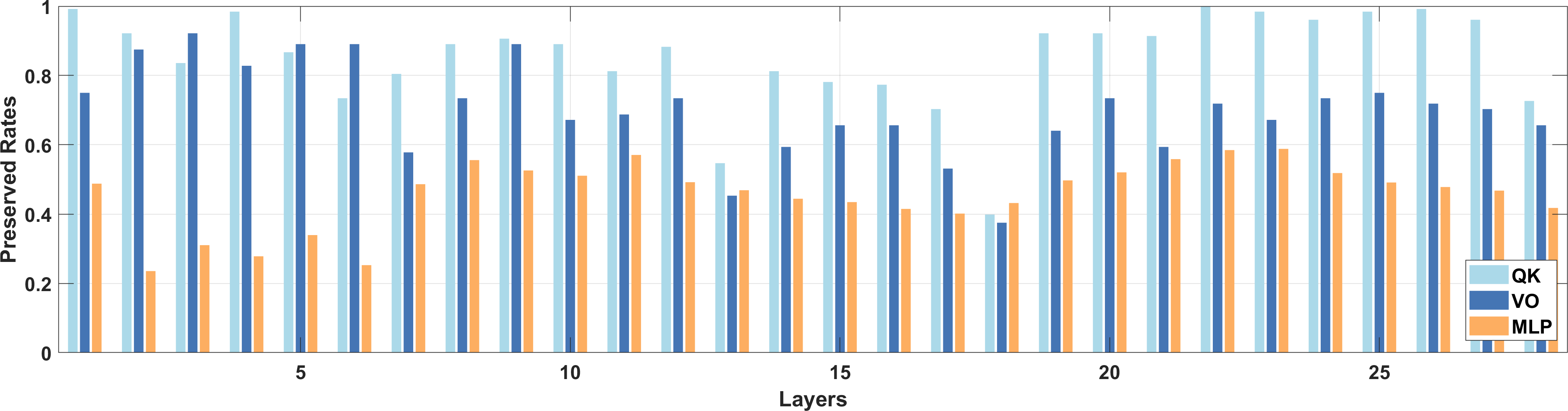
Figure 4: Model width after ToMoE for the Qwen-2.5 7B model when the number of active parameters equals 50%.

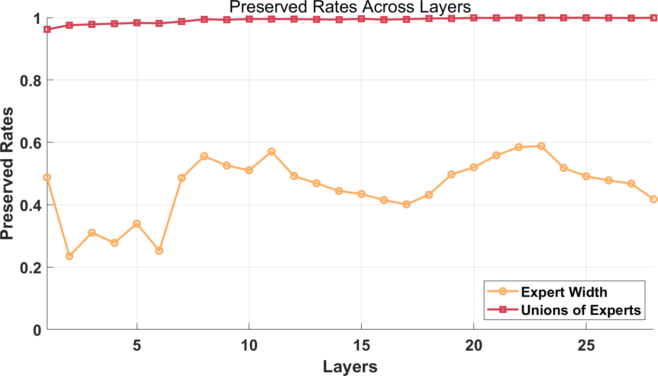
(a)

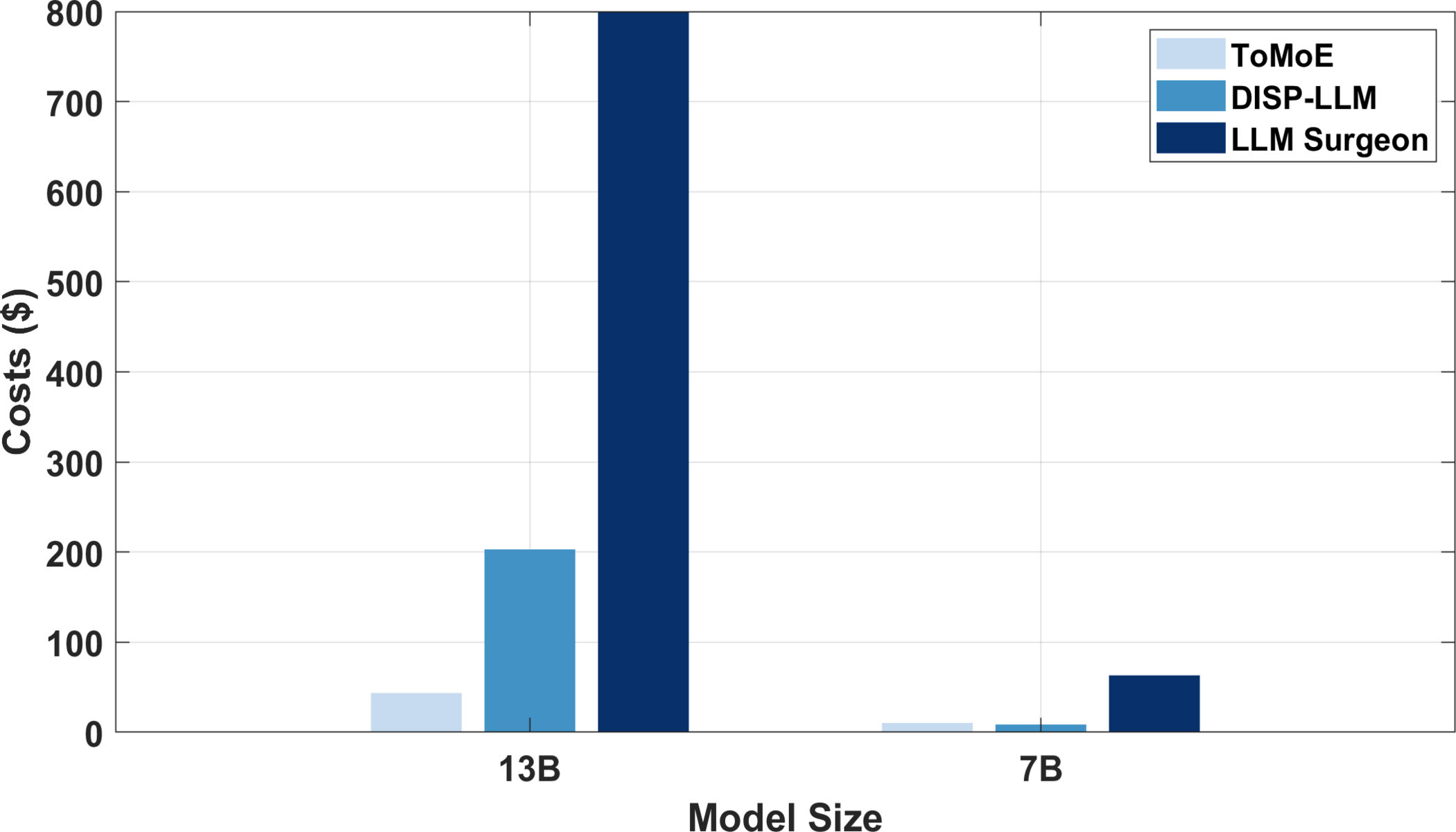
(b)

Figure 5: (a) Model width and the union of all experts. (b) Costs of different learning-based methods.

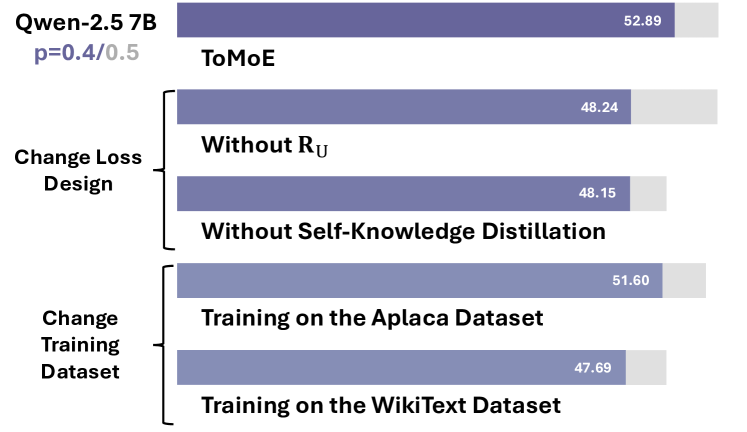
Figure 6: Ablation Study on Qwen-2.5 7B.

Tab. 1 presents the perplexity results of structured pruning methods applied to LLaMA-2 models of sizes 7B and 13B on the WikiText-2 dataset, comparing various methods with 70%, 60%, and 50% of active parameters which correspond to pruning ratios of 30%, 40%, and 50% for pruning. Across all pruning ratios, ToMoE consistently achieves the lowest perplexity compared to other methods, even outperforming many approaches with significantly larger numbers of active parameters. For instance, ToMoE with 50% active parameters achieves a perplexity of 8.36, which is superior to LLM-Pruner, ShortGPT, SLEB, and SliceGPT at a 30% pruning ratio. Furthermore, ToMoE with 50% active parameters surpasses ModeGPT and LLM Surgeon at a 40% pruning ratio. While the gap between ToMoE and DISP-LLM is smaller, it is still obvious at a 50% pruning ratio: ToMoE achieves a perplexity that is 1.48 points lower than DISP-LLM. ToMoE also exhibits superior performance with the LLaMA-2 13B model, maintaining a similar advantage over other methods as observed with the LLaMA-2 7B model. This demonstrates the effectiveness of ToMoE in maintaining strong language modeling performance, even with much fewer active parameters. Tab. 2 presents a comparison of our method against semi-structural pruning techniques. Our approach consistently achieves the lowest perplexity while retaining 50% of the active parameters. Moreover, the performance gap between our method and the semi-structural pruning methods is also obvious. On the LLaMA-2 7B model, SparseGPT achieves the second-best performance, with our method improving upon it by 1.81 in terms of perplexity. For the LLaMA-2 13B model, Pruner-Zero shows the second-best performance, while ToMoE further reduces the perplexity by 0.63. The comparison against seme-structural pruning methods further demonstrates the advantage of our method on the language modeling task.

4.3 Zero-Shot Performance

In Tab. 3, we present the zero-shot performance of various methods on LLaMA-2 7B, LLaMA-3 8B, and Qwen-2.5 7B. Our method consistently achieves the best average performance across all models. Compared to relatively weaker methods like ShortGPT and SliceGPT, our approach demonstrates higher average performance (ToMoE 50%: 56.07 vs. SliceGPT 70%: 53.73 and ShortGPT 70%: 53.25) while utilizing 20% fewer active parameters on the LLaMA-2 7B model. Against stronger baselines such as LLM Surgeon and DISP-LLM, ToMoE achieves better performance with 10% fewer active parameters on the same model. For instance, ToMoE (50%) outperforms LLM Surgeon (60%), and ToMoE (60%) outperforms both LLM Surgeon (70%) and DISP-LLM (70%). Although ModeGPT performs closer to ToMoE, the gap remains significant. With 60% active parameters, ToMoE is 3.14 better than ModeGPT. In addition, when keeping 50% active parameters, ToMoE outperforms DISP-LLM and LLM Surgeon by 5.02 and 10.39, respectively. The performance advantage of ToMoE is even larger on LLaMA-3 8B, where it reduces 5% more active parameters than ModeGPT while still achieving a 2.71 performance gain. Furthermore, when removing 15% more active parameters compared to ShortGPT and SliceGPT, ToMoE exceeds their average performance by 18.93 and 16 points, respectively.

For Qwen-2.5 7B, ToMoE significantly outperforms DISP-LLM, consistent with previous findings on other models. We further investigate the effect of the number of experts $N$ when 40% to 50% of the parameters are active. The results indicate that increasing the number of experts to 16 is beneficial. However, further increasing $N$ to 24 provides only marginal or no improvement, likely because a too-large number of experts burdens the learning process.

4.4 Analysis of ToMoE

Training Dynamics. In Fig.3, we visualize the training dynamics under different values of $p$. Across all $p$, the knowledge distillation loss $\mathcal{L}$ (Fig.3(a)), the parameter regularization loss $\mathcal{R}_{\text{P}}$, and the union of experts regularization loss $\mathcal{R}_{\text{U}}$ decrease over the course of training. Notably, the parameter regularization loss quickly drops to $0$ in the early stages of training, while using a smaller $p$ requires more iterations. The peak of the union of experts regularization loss increases when using smaller values of $p$, indicating that the initial solution tends to only cover a small portion of the dense model. Regarding the load balancing loss, it oscillates around 0.15, demonstrating that ToMoE maintains a relatively balanced load distribution during the training process.

Ablation Study. In Fig. 6, we present the average zero-shot task performance under different settings. For $p=0.4$ and $p=0.5$, replacing the knowledge distillation loss with the language modeling loss significantly impacts performance. At $p=0.4$, removing $\mathcal{R}_{\text{U}}$ also results in a substantial performance drop, whereas the impact is much smaller at $p=0.5$. We hypothesize that this difference arises because reducing $p$ makes the learning process more challenging. Without the guidance provided by $\mathcal{R}_{\text{U}}$, the model struggles to effectively utilize the parameters of the original model. Additionally, the choice of dataset affects performance, particularly when switching to the WikiText dataset. This demonstrates that a mixing dataset is beneficial to the overall performance.

Other Analysis. (1). We present the width of our ToMoE model for Qwen-2.5 7B in Fig. 4. We can see that the layer-wise configuration is highly non-uniform, showing that our method can flexibly set the width of different layers and operations. (2). In Fig. 5(a), we show that the union of experts is close to the full model capacity even though the width of experts across different layers is highly non-uniform, demonstrating the effectiveness of our loss design. (3). In Fig. 5(b), we show the costs of different learning-based methods in terms of US dollars. ToMoE has a similar cost compared to DISP-LLM with LLaMA-2 7B and 13B models, and both of them are much cheaper than LLM Surgeon. (4). Finally, we visualize the expert selection for LLaMA-2 7B in Tab. 4. We can see that each expert aligns syntax rather than semantic meanings resembling the observations in (Jiang et al., 2024).

5 Conclusion

In this paper, we propose a novel algorithm, ToMoE, for converting dense models into MoE models through dynamic structural pruning. The resulting MoE models significantly outperform state-of-the-art structural pruning methods while using similar or lower training costs compared to other learning-based pruning methods. Our findings reveal the presence of meaningful experts within the MLP layers of dense models, even without fine-tuning the model weights. ToMoE serves as a powerful tool for uncovering these experts within the original dense LLM.

Impact Statement

This paper introduces a method to reduce the active parameters of LLMs during inference, thereby lowering their computational costs. By improving efficiency, it can lead to a decrease in carbon emissions, contributing to environmental sustainability and benefiting society and industry alike. Additionally, reducing the costs associated with LLMs could make their services more affordable, broadening access to powerful AI tools and ensuring that AI development remains inclusive and widely accessible.

Appendix A Details of trainable modules

A.1 Module Configurations

Module Types	Removed?	Structures
HyperNetwork	✓	Input $z$ $\rightarrow$ Bi-GRU(32,64)
$\text{Proj}_{\text{E}}^{\text{\tiny MHA}}$	✗	Linear($d$, $d_{e}$ = 128)
$\text{Proj}_{\text{D}}^{\text{\tiny MHA}}$	✗	LayerNorm($d_{e}$ = 128)$\rightarrow$ GeLU$\rightarrow$Linear($d_{e}$ = 128, $\frac{d}{H}$)
$\text{Proj}_{\text{D}}^{\text{\tiny MLP}}$	✓	LayerNorm($d_{e}$ = 128)$\rightarrow$ GeLU$\rightarrow$Linear($d_{e}$ = 128, $d_{\text{mid}}$)
Router	✗	Linear($d$, $N$)

Table 5: Detailed configuration of trainable modules.

We present the details of trainable modules in Tab. 5. In short, we project the input tokens to a low-dimensional space and add them to the output of the HyperNetwork. The input $z$ to the HyperNetwork are fixed random vectors of size $N\times 32$ sampled from Normal Distribution. Except for the HyperNetwork, other individual trainable modules are created for each MHA and MLP layer. If we have $L$ blocks, then we will have $L$ $\text{Proj}_{\text{E}}^{\text{\tiny MHA}}$, $L$ $\text{Proj}_{\text{D}}^{\text{\tiny MHA}}$ with output size of $\frac{d}{H}$, $L$ $\text{Proj}_{\text{D}}^{\text{\tiny MHA}}$ with output size of $\frac{d}{2H}$ $L$, $\text{Proj}_{\text{D}}^{\text{\tiny MLP}}$ and $L$ Router layers. Notations of $d$, $H$, $d_{\text{mid}}$, and $N$ are already defined in Sec. 2.

After we complete the training of ToMoE, we do not have to preserve all modules. The embeddings from the HyperNetwork will be saved, so the HyperNetwork can be removed without impacting the model. $\text{Proj}_{\text{D}}^{\text{\tiny MLP}}$ brings most additional parameters, fortunately, it can also be removed. After the training of ToMoE, $\mathbf{E}$ and $\text{Proj}_{\text{D}}^{\text{\tiny MLP}}$ can be used to directly generate experts:

$$~\mathbf{s}_{\scriptstyle{\mathbf{e}}}=\text{ST-GS}(\text{Proj}_{\text{D}}^{\text{\tiny MLP}}(\mathbf{E})),$$ (11)

where ST-GS again is the Straight-Through Gumbel-Sigmoid function. $\mathbf{s}_{\scriptstyle{\mathbf{e}}}\in\{0,1\}^{N\times d_{\text{mid}}}$ is the resulting binary vectors to select experts from the dense model. Once $\mathbf{s}_{\scriptstyle{\mathbf{e}}}$ is generated, it can be reused and thus we no longer need $\text{Proj}_{\text{D}}^{\text{\tiny MLP}}$. Let $\mathbf{S}_{\scriptstyle{\mathbf{e}}}^{i}=\text{Diag}(\mathbf{s}_{\scriptstyle{\mathbf{e}}}^{i}),\ i=1,\cdots,N$. Similarly, we use $\hat{\mathbf{s}}_{\scriptstyle{\mathbf{e}}}^{i}\in\Re^{d_{\text{mid}}\times d_{\text{mid}}^{\prime}}$ to represent the actual column or row selection matrix by removing zero columns or rows, where $d_{\text{mid}}^{\prime}<d_{\text{mid}}$ and it is the width of each expert. The $i$th expert can be represented as:

$$f_{\text{MLP}}^{i}(\mathbf{X})=\sigma(\mathbf{X}\mathbf{W}_{G}\hat{\mathbf{S}}_{\scriptstyle{\mathbf{e}}}^{i})\odot(\mathbf{X}\mathbf{W}_{U}\hat{\mathbf{S}}_{\scriptstyle{\mathbf{e}}}^{i})\hat{\mathbf{S}}_{\scriptstyle{\mathbf{e}}}^{i}\mathbf{W}_{D}.\\$$ (12)

After ToMoE, given the result of the routing function $\mathbf{G}={\text{ST-G}}(\text{Router}(\mathbf{X}))$, the MLP calculation with MoE can be written as:

$$\mathbf{Y}_{t}=\mathbf{G}_{t,i}f_{\text{MLP}}^{i}(\mathbf{X}_{t}),~$$ (13)

where $\mathbf{X}_{t}$ is the feature map of $t$th token, and $i$ represents the index where $\mathbf{G}_{t,i}=1$. Note that Eq. 13 is still differentiable with respect to the parameters of the Router.

Another question is how many parameters we need after introducing Top-K routing for MHA layers and Top-1 routing for MLP layers. Analytically, the additional parameters can be calculated by $L\times d\times 128+L\times 128\times(\frac{d}{H})+L\times d\times N$. Let’s use LLaMA-2 7B as an example, $L=32$, $d=4096$, $N=8$, $H=32$, the additional parameters are $1\times 32\times 4096\times 128+32\times 128\times(128)+32\times 4096\times 8=0.0184$B. This is equivalent to $0.27\%$ of the total parameters of the LLaMA-2 7B model, and thus the additional parameter is not significant compared to the original number of parameters.

A.2 Head Dimension Pruning vs. RoPE

Rotary Position Embedding (RoPE) (Su et al., 2024) is a popular positional encoding method and it is regularly used in LLMs like LLaMA (Touvron et al., 2023b). RoPE divides the $\frac{d}{H}$ dimensional space into $\frac{d}{2H}$ sub-spaces, and they are applied on query and key. This means that if we want to perform head dimension pruning for query and key matrices, we need to follow the sub-spaces resulting from RoPE and make these two sub-spaces share the same pruning mask $\mathbf{s}_{0}$, and the final pruning mask for query and key is $\mathbf{s}_{0}^{\prime}=[{\mathbf{s}_{0}}_{[1:\frac{d}{2H}]},{\mathbf{s}_{0}}_{[1:\frac{d}{2H}]}]$, and clearly the size of ${\mathbf{s}_{0}}_{[1:\frac{d}{2H}]}$ is $\frac{d}{2H}$. In short, we simply select the first half of elements from $\mathbf{s}_{0}$ and repeat it twice to have the final pruning decision. We also found that applying dynamic pruning for query and key matrices along the head dimension is difficult and unreasonable since different tokens may have different positions after pruning. It becomes a problem when calculating the inner product between the query and key matrices given different tokens.

By applying head dimension pruning, our method also does not need to be modified when facing different attention mechanisms like GQA (Grouped-Query Attention) (Ainslie et al., 2023) and MQA (Multi-Query Attention) (Shazeer, 2019).

Table 6: Zero-shot task performance of compressed LLaMA-2 13B and Qwen-2.5 14B.

Model	Active Parameters	Method	ARC-e	ARC-c	PIQA	WinoG.	HellaS.	Average
			acc-norm	acc-norm	acc-norm	acc	acc-norm
LLaMA-2 13B	100%	Dense	77.48	49.23	80.47	72.22	79.39	71.76
	70%	SliceGPT (Ashkboos et al., 2024)	60.27	36.18	69.42	64.09	49.74	55.94
		LLM Surgeon (van der Ouderaa et al., 2024)	69.74	40.27	76.50	68.67	71.52	65.34
		DISP-LLM (Gao et al., 2024)	63.80	39.42	74.43	66.85	70.86	63.07
		DISP-LLM Alpaca (Gao et al., 2024)	68.98	44.28	77.31	67.32	68.98	65.59
		MoDeGPT-Alpaca (Lin et al., 2024)	70.24	41.47	77.15	71.27	71.84	66.39
		ToMoE (Ours)	74.58	45.14	77.97	75.44	68.19	68.26
	60%	SliceGPT (Ashkboos et al., 2024)	48.99	32.51	63.17	56.75	39.85	48.25
		LLM Surgeon (van der Ouderaa et al., 2024)	63.80	37.12	73.16	65.75	65.64	60.94
		DISP-LLM (Gao et al., 2024)	62.67	35.63	73.39	62.67	65.86	60.04
		DISP-LLM Alpaca (Gao et al., 2024)	66.79	42.75	75.30	64.25	67.52	63.32
		MoDeGPT-Alpaca (Lin et al., 2024)	63.72	38.82	71.87	66.30	62.10	60.56
		ToMoE (Ours)	67.63	41.81	75.79	66.38	73.41	65.00
	50%	LLM Surgeon (van der Ouderaa et al., 2024)	56.19	37.12	68.87	63.22	56.19	56.32
		DISP-LLM (Gao et al., 2024)	58.27	36.87	68.67	59.27	57.18	54.50
		DISP-LLM Alpaca (Gao et al., 2024)	55.72	37.54	72.20	59.59	62.39	57.49
		ToMoE (Ours)	63.51	37.97	73.29	62.59	68.30	61.13
Qwen-2.5 14B	100%	Dense	79.42	59.13	83.09	74.98	82.10	75.74
	50%	DISP-LLM (Gao et al., 2024)	65.87	37.99	72.20	58.51	60.63	59.04
		ToMoE (Ours)	66.37	39.16	74.59	60.69	65.57	61.28
	40%	DISP-LLM (Gao et al., 2024)	56.36	32.62	70.08	54.22	51.50	52.96
		ToMoE (Ours)	59.85	34.73	71.49	57.62	56.60	56.06

A.3 Details of Gumbel-Softmax and Gumbel-Sigmoid

The Gumbel-Softmax function (Jang et al., 2016) allows for differentiable sampling from a categorical distribution. Given logits $\mathbf{x}$, the Gumbel-Softmax sample $\mathbf{y}$ is computed as:

$$\mathbf{y}=\text{softmax}\left(\frac{\mathbf{x}+\mathbf{g}}{\tau}\right),$$

where each element of $\mathbf{g}$ is drawn from $\text{Gumbel}(0,1)$, and $\tau$ is the temperature parameter that controls the smoothness of the distribution. Combining Gumbel-Softmax with the Straight-Through gradient Estimator (Bengio et al., 2013), we have the following equation:

$$~\text{ST-G}(\mathbf{x})=\text{one-hot}\left(\arg\max_{i\in D}\left[\frac{x_{i}+g_{i}}{\tau}\right]\right)$$ (14)

where $D=\{1,2,\cdots,N\}$, $N$ again is the number of experts in our setting, and one-hot will assign $1$ corresponding to the position of the maximum value in $\frac{\mathbf{x}+\mathbf{g}}{\tau}$ and assign $0$ to other positions.

The Gumbel-Sigmoid function is a special case of the Gumbel-Softmax function, designed for binary distributions. Given logits $\mathbf{x}$, the Gumbel-Sigmoid sample $y$ is computed as:

$$y=\text{sigmoid}\left(\frac{\mathbf{x}+\mathbf{g}}{\tau}\right),$$

where $\mathbf{g}$ is sampled from $\text{Gumbel}(0,1)$ and $\tau$ again is the temperature parameter. Combining with the Straight-Through gradient Estimator, we have the following equation:

$$~\text{ST-GS}(\mathbf{x})=\text{round}(\text{sigmoid}\left(\frac{\mathbf{x}+\mathbf{g}+b}{\tau}\right)),$$ (15)

where $b$ is a constant bias in our implementation and it ensures that all experts start from the whole model, $\text{round}(\cdot)$ will round the input values to the nearest integer, and in our case, it rounds inputs to $0$ or $1$. For all experiments, we set $b=3.0$ in Eq. 15, and we set $\tau=0.4$ for Eq. 14 and Eq. 15.

Table 7: Zero-shot task performance of the compressed Phi-2.

Active Parameters	Method	ARC-e	ARC-c	PIQA	WinoG.	HellaS.	Avg
		acc-norm	acc-norm	acc-norm	acc	acc-norm
100%	Dense	78.24	54.01	79.11	75.61	73.86	72.17
80%	SliceGPT (Ashkboos et al., 2024)	58.00	35.32	71.87	67.80	57.76	58.15
	+Fine-tuning	56.61	38.91	71.27	67.17	54.86	57.76
	DISP-LLM (Gao et al., 2024)	68.18	44.11	74.86	67.09	62.93	63.43
75%	SliceGPT (Ashkboos et al., 2024)	53.70	31.66	69.21	65.35	52.40	54.46
	+Fine-tuning	52.78	35.49	69.91	65.19	52.48	55.17
	DISP-LLM (Gao et al., 2024)	65.93	43.34	74.27	65.11	59.95	61.72
70%	SliceGPT (Ashkboos et al., 2024)	53.03	30.29	65.94	63.14	47.56	51.99
	+Fine-tuning	46.38	32.68	66.16	63.54	49.72	51.70
	DISP-LLM (Gao et al., 2024)	63.59	38.48	73.34	65.19	54.43	59.00
	ToMoE (Ours)	70.79	43.86	77.09	66.38	62.68	64.16

Appendix B More Details of the Loss Design

B.1 Implementation of the Self-Knowledge Distillation

During the ToMoE learning process, we freeze the parameters of the original model. This approach offers the additional benefit of enabling self-knowledge distillation without the need to load an extra model. In Lst. LABEL:lst:self-kd, we present the pseudo-code for the self-knowledge distillation process. In summary, we first disable the trainable modules associated with ToMoE and compute the output logits from the original model. Next, we re-enable the trainable modules for ToMoE and perform a regular forward pass. The logits from the original model are then used to guide the learning of ToMoE.

Listing 1: Pseudo-code for self-knowledge distillation.

⬇

1with torch.no_grad():

2 # Disable trainable modules for ToMoE

3 helper.set_module_status(model, False)

4

5 # Get logits from the teacher (original model)

6 teacher_output = model(inputs)

7 teacher_logits = teacher_output.logits

8

9 # Enable trainable modules for ToMoE

10 helper.set_module_status(model, True)

11

12# Get logits from the student model from ToMoE learning process

13model_output = model(inputs)

14logits = model_output.logits

Table 8: ToMoE Visualization of LLaMA-2 7B with 50% active parameters

Expert Color	Expert 1 Expert 2 Expert 3 Expert 4 Expert 5 Expert 6 Expert 7 Expert 8
MLP 1	<s> Homarus gammarus, known as the European lobster or common lobster, is a species of clawed lobster from the eastern Atlantic Ocean, Mediterranean Sea and parts of the Black Sea. It is closely related to the American lobster, H. americanus. It may grow to a length of 60 cm (24 in) and a mass of 6 kilograms (13 lb), and bears a conspicuous pair of claws. In life, the lobsters are blue, only becoming ’lobster red’ on cooking. Mating occurs in the summer, producing eggs which are carried by the females for up to a year before hatching into planktonic larvae. Homarus gammarus is a highly esteemed food, and is widely caught using lobster pots, mostly around the British Isles.
MLP 16	<s> Homarus gammarus, known as the European lobster or common lobster, is a species of clawed lobster from the eastern Atlantic Ocean, Mediterranean Sea and parts of the Black Sea. It is closely related to the American lobster, H. americanus. It may grow to a length of 60 cm (24 in) and a mass of 6 kilograms (13 lb), and bears a conspicuous pair of claws. In life, the lobsters are blue, only becoming ’lobster red’ on cooking. Mating occurs in the summer, producing eggs which are carried by the females for up to a year before hatching into planktonic larvae. Homarus gammarus is a highly esteemed food, and is widely caught using lobster pots, mostly around the British Isles.
MLP 32	<s> Homarus gammarus, known as the European lobster or common lobster, is a species of clawed lobster from the eastern Atlantic Ocean, Mediterranean Sea and parts of the Black Sea. It is closely related to the American lobster, H. americanus. It may grow to a length of 60 cm (24 in) and a mass of 6 kilograms (13 lb), and bears a conspicuous pair of claws. In life, the lobsters are blue, only becoming ’lobster red’ on cooking. Mating occurs in the summer, producing eggs which are carried by the females for up to a year before hatching into planktonic larvae. Homarus gammarus is a highly esteemed food, and is widely caught using lobster pots, mostly around the British Isles.

B.2 Efficient Implementation of $\mathcal{R}_{\mathbf{u}}$

Recall from Eq. 6 that the union regularization for MLP and MHA layers is defined as:

$$\mathcal{R}_{\mathbf{u}}=\bigcup_{i=1}^{T}\mathbf{s}_{i}=1-\prod_{i=1}^{T}(1-\mathbf{s}_{i}).$$

For MLP layers, this equation incurs high computational costs since $\mathbf{s}\in\mathbb{R}^{T\times d_{\text{mid}}}$, whereas for MHA layers, the cost is significantly lower because $\frac{d}{H}\ll d_{\text{mid}}$. To simplify Eq. 6, note that all $\mathbf{s}_{i}$ ($i=1,\ldots,T$) are derived from $N$ experts. Using embeddings from the hypernetwork, we calculate the configuration of $N$ experts as:

$$\mathbf{s}_{\mathbf{e}}=\text{ST-GS}(\text{Proj}_{\text{D}}^{\text{\tiny MLP}}(\mathbf{E})),$$

and substitute $\mathbf{s}_{\mathbf{e}}$ into Eq. 6:

$$~\mathcal{R}_{\mathbf{u}}^{\text{\tiny MLP}}=\bigcup_{i=1}^{N}\mathbf{s}_{\scriptstyle{\mathbf{e}}}^{i}=1-\prod_{i=1}^{N}(1-\mathbf{s}_{\scriptstyle{\mathbf{e}}}^{i}).$$ (16)

This reduces computation by a factor of $\frac{T}{N}$. For example, in LLaMA-2, the computational cost is reduced by $\frac{2048}{8}=256$ times.

B.3 Equivalence of MoE and pseudo-MoE

One major challenge when training MoE models is maintaining an appropriate expert capacity, defined as the number of tokens each expert processes (Fedus et al., 2022). This is typically addressed using a load balancing loss. Without this loss, some experts may become overloaded while others remain underutilized, leading to bottlenecks where a few experts dominate the computation.

Although ToMoE also requires load balancing loss, the potential overhead introduced by load balancing is mitigated by the pseudo-MoE approach after ToMoE. After applying ToMoE, the resulting model can be trained using pseudo-MoE, which resembles the training of a dense model. This is straightforward to implement as follows:

$$f_{\text{MLP}}(\mathbf{X})=\sigma(\mathbf{X}\mathbf{W}_{G}){\mathbf{S}}\odot(\mathbf{X}\mathbf{W}_{U}{\mathbf{S}}){\mathbf{S}}\mathbf{W}_{D},$$ (17)

where $\mathbf{S}_{i}$ in $\mathbf{S}$ represents the routed expert from $\mathbf{S}_{e}$ in Eq. 11, as determined by the router. The pseudo-MoE is useful when the active number of parameters is relatively large. In such cases, pseudo-MoE training can be more time-efficient than conventional MoE training.

Appendix C More Implementation Details

During training the modules of ToMoE, we use AdamW optimizer to optimize it with a constant learning rate $10^{-3}$ and weight decay $0.05$. For different models, we always set the mini-batchsize to $1$ on each GPU. For LLaMA-2 7B, and Qwen-2.5 7B models, we use 2 NVIDIA A100 GPUs, For LLaMA-3 8B, we use 3 NVIDIA A100 GPUs. For LLaMA-2 13B and Qwen-2.5 14B models, we use 4 NVIDIA A100 GPUs. For all the rest models, we use 1 NVIDIA A100 GPU. We set $p=\{0.6,0.5,0.4,0.3\}$ when the ratios of active parameters equals to $\{40\%,50\%,60\%,70\%\}$.

For the Alpaca dataset , we use the ‘text’ column within the dataset which combines the columns of ‘instruction’ and ‘output’. For the Code Alpaca dataset , we combine the ‘instruction’, ‘input’, and ‘output’ columns as one training sample.

Table 9: ToMoE Visualization of LLaMA-2 7B with 50% active parameters (continued).

Expert Color	Expert 1 Expert 2 Expert 3 Expert 4 Expert 5 Expert 6 Expert 7 Expert 8
MLP 1	<s> Find the equation of the line passing through the points (3, 5) and (7, 9) using the slope-intercept form of a linear equation. To find the equation of the line passing through the points (3, 5) and (7, 9) using the slope-intercept form (y = mx + b), we first need to find the slope (m) and the y-intercept (b). 1. Find the slope (m): m = (y2 - y1) / (x2 - x1) m = (9 - 5) / (7 - 3) m = 4 / 4 m = 1 2. Use one of the points to find the y-intercept (b). We’ll use (3, 5): y = mx + b 5 = 1 * 3 + b 5 = 3 + b b = 2 3. Write the equation in slope-intercept form: y = mx + b y = 1x + 2 y = x + 2 The equation of the line passing through the points (3, 5) and (7, 9) is y = x + 2.
MLP 16	<s> Find the equation of the line passing through the points (3, 5) and (7, 9) using the slope-intercept form of a linear equation. To find the equation of the line passing through the points (3, 5) and (7, 9) using the slope-intercept form (y = mx + b), we first need to find the slope (m) and the y-intercept (b). 1. Find the slope (m): m = (y2 - y1) / (x2 - x1) m = (9 - 5) / (7 - 3) m = 4 / 4 m = 1 2. Use one of the points to find the y-intercept (b). We’ll use (3, 5): y = mx + b 5 = 1 * 3 + b 5 = 3 + b b = 2 3. Write the equation in slope-intercept form: y = mx + b y = 1x + 2 y = x + 2 The equation of the line passing through the points (3, 5) and (7, 9) is y = x + 2.
MLP 32	<s> Find the equation of the line passing through the points (3, 5) and (7, 9) using the slope-intercept form of a linear equation. To find the equation of the line passing through the points (3, 5) and (7, 9) using the slope-intercept form (y = mx + b), we first need to find the slope (m) and the y-intercept (b). 1. Find the slope (m): m = (y2 - y1) / (x2 - x1) m = (9 - 5) / (7 - 3) m = 4 / 4 m = 1 2. Use one of the points to find the y-intercept (b). We’ll use (3, 5): y = mx + b 5 = 1 * 3 + b 5 = 3 + b b = 2 3. Write the equation in slope-intercept form: y = mx + b y = 1x + 2 y = x + 2 The equation of the line passing through the points (3, 5) and (7, 9) is y = x + 2.

Appendix D More Experimental Results

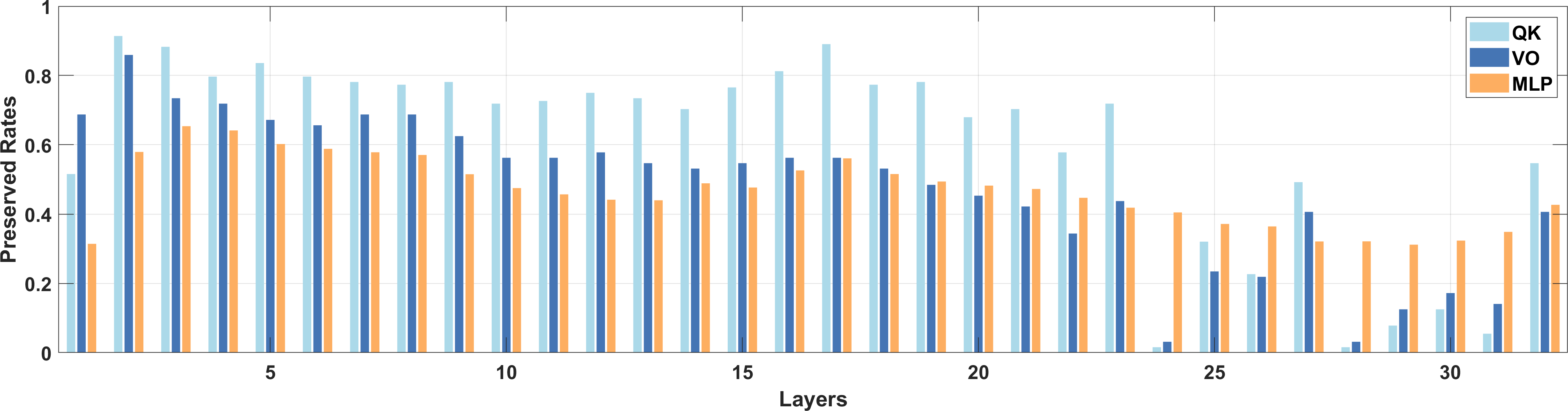
Figure 7: Model width after ToMoE for the LLaMA-2 7B model when the number of active parameters equals 50%.

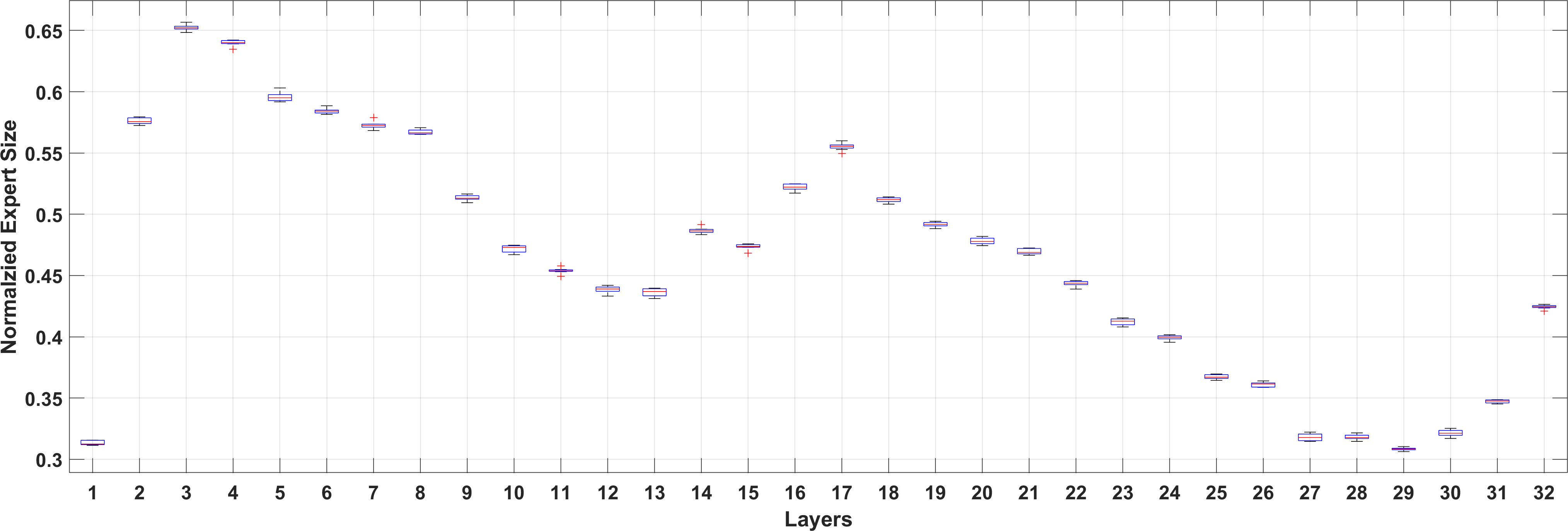
Figure 8: Box plot of widths across different experts for the LLaMA-2 7B model when the number of active parameters equals 50%.

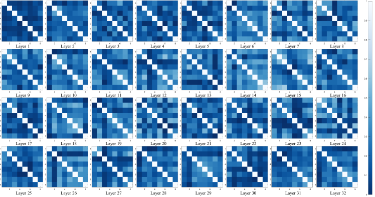
Figure 9: The similarity of different experts from different layers of ToMoE of the LLaMA-2 7B model.

In Tab. 6 and Tab. 7, we present the zero-shot performance of various methods on LLaMA-2 13B, Qwen-2.5 14B, and Phi-2 models. From Tab. 6, it is evident that ToMoE consistently outperforms other methods. Compared to 7B or 8B models, the performance gap between our method and other approaches is smaller, which also holds for the differences between baseline methods. This is likely due to the larger model sizes.

On the LLaMA-2 13B model, ToMoE surpasses structural pruning methods even with smaller compression rates. For instance, ToMoE with 50% active parameters performs better than MoDeGPT and LLM Surgeon with a 40% compression rate. The performance gap becomes even more obvious when comparing methods with the same number of active parameters. Similarly, from Tab. 7, ToMoE demonstrates superior performance compared to SliceGPT and DISP-LLM. Specifically, ToMoE with 70% active parameters achieves better results than all three compression levels of SliceGPT and DISP-LLM.

In Fig. 7, we illustrate the width of ToMoE for the LLaMA-2 7B model. A highly non-uniform pattern emerges in the allocation of active parameters, indicating that ToMoE can effectively determine the ideal distribution of active parameters, even when the allocation is highly non-uniform.

These results highlight the effectiveness of ToMoE in preserving the capacity of LLMs compared to structural pruning methods. Additionally, they demonstrate that ToMoE performs robustly across various scales and types of LLMs.

Appendix E Visualization of Experts

In this section, we analyze the properties of the experts produced by our method. Tab. 8 and Tab. 9 present visualizations of the routed tokens among experts across different layers and input texts.

In Tab. 8, we observe no distinct patterns in the allocation of tokens to specific experts, which aligns with our observations in Tab. 4. An interesting trend emerges when comparing layers: the first layer exhibits a more diverse token distribution, while subsequent layers prefer to assign continuous tokens to the same expert. Tab. 9 focuses on inputs related to a math problem. Unlike the visualization in Tab. 8, the MoE routing for the math problem reveals clearer semantic patterns. For instance, Expert 2 in MLP 16 is predominantly activated by numbers and mathematical notations, and a similar behavior is observed for Expert 8 in MLP 32. This suggests that the experts in ToMoE may encode more distinct semantic meanings compared to MoE models trained from scratch. Further investigation is required to fully understand the precise semantic roles of ToMoE experts.

In Fig. 8, we present a box plot showing the expert sizes across different layers. The figure reveals that the maximum and minimum expert sizes are closely aligned across layers. This outcome is a direct result of applying constraints from Eq. 8 and Eq. 9, as well as only penalizing the largest expert in Eq. 8. During training, minimizing the task loss (self-knowledge distillation loss) encourages experts to grow in size. Consequently, smaller experts do not remain small due to the task loss and they are not penalized by the parameter regularization loss. This iterative process leads to all experts eventually converging to similar sizes. After completing the ToMoE training process, we adjust the width of all experts to match the maximum size among them. This ensures uniform computational cost across all experts.

In Fig. 9, we present a visualization of the similarity between different experts across all layers of the LLaMA-2 7B model. Within the same layer, experts generally exhibit comparable similarity values, indicating that while the experts share the same size, their weights remain distinct. Notably, certain layers, such as layer 1 and layer 30, show lower similarity values. This observation aligns with expectations, as the expert sizes in these layers are smaller.

References

- Ainslie et al. (2023) Ainslie, J., Lee-Thorp, J., de Jong, M., Zemlyanskiy, Y., Lebron, F., and Sanghai, S. Gqa: Training generalized multi-query transformer models from multi-head checkpoints. In Proceedings of the 2023 Conference on Empirical Methods in Natural Language Processing, pp. 4895–4901, 2023.
- Anagnostidis et al. (2023) Anagnostidis, S., Pavllo, D., Biggio, L., Noci, L., Lucchi, A., and Hofmann, T. Dynamic context pruning for efficient and interpretable autoregressive transformers. In Oh, A., Naumann, T., Globerson, A., Saenko, K., Hardt, M., and Levine, S. (eds.), Advances in Neural Information Processing Systems 36: Annual Conference on Neural Information Processing Systems 2023, NeurIPS 2023, New Orleans, LA, USA, December 10 - 16, 2023, 2023. URL http://papers.nips.cc/paper_files/paper/2023/hash/cdaac2a02c4fdcae77ba083b110efcc3-Abstract-Conference.html.
- Anthropic (2023) Anthropic. Claude: A safer conversational ai assistant. https://www.anthropic.com/index/2023/02/claude, 2023.
- Anwar et al. (2017) Anwar, S., Hwang, K., and Sung, W. Structured pruning of deep convolutional neural networks. ACM J. Emerg. Technol. Comput. Syst., 13(3):32:1–32:18, 2017. doi: 10.1145/3005348. URL https://doi.org/10.1145/3005348.
- Ashkboos et al. (2024) Ashkboos, S., Croci, M. L., do Nascimento, M. G., Hoefler, T., and Hensman, J. Slicegpt: Compress large language models by deleting rows and columns. In The Twelfth International Conference on Learning Representations, 2024.
- Bengio et al. (2013) Bengio, Y., Léonard, N., and Courville, A. Estimating or propagating gradients through stochastic neurons for conditional computation. arXiv preprint arXiv:1308.3432, 2013.
- Bisk et al. (2020) Bisk, Y., Zellers, R., Gao, J., Choi, Y., et al. Piqa: Reasoning about physical commonsense in natural language. In Proceedings of the AAAI conference on artificial intelligence, volume 34, pp. 7432–7439, 2020.
- Brown (2020) Brown, T. B. Language models are few-shot learners. arXiv preprint arXiv:2005.14165, 2020.
- Chen et al. (2020) Chen, Y., Dai, X., Liu, M., Chen, D., Yuan, L., and Liu, Z. Dynamic convolution: Attention over convolution kernels. In Proceedings of the IEEE/CVF Conference on Computer Vision and Pattern Recognition, pp. 11030–11039, 2020.
- Clark et al. (2018) Clark, P., Cowhey, I., Etzioni, O., Khot, T., Sabharwal, A., Schoenick, C., and Tafjord, O. Think you have solved question answering? try arc, the ai2 reasoning challenge. arXiv preprint arXiv:1803.05457, 2018.
- Dai et al. (2024) Dai, D., Deng, C., Zhao, C., Xu, R., Gao, H., Chen, D., Li, J., Zeng, W., Yu, X., Wu, Y., et al. Deepseekmoe: Towards ultimate expert specialization in mixture-of-experts language models. arXiv preprint arXiv:2401.06066, 2024.
- Dong et al. (2024a) Dong, H., Yang, X., Zhang, Z., Wang, Z., Chi, Y., and Chen, B. Get more with LESS: synthesizing recurrence with KV cache compression for efficient LLM inference. In Forty-first International Conference on Machine Learning, ICML 2024, Vienna, Austria, July 21-27, 2024. OpenReview.net, 2024a. URL https://openreview.net/forum?id=uhHDhVKFMW.
- Dong et al. (2024b) Dong, P., Li, L., Tang, Z., Liu, X., Pan, X., Wang, Q., and Chu, X. Pruner-zero: Evolving symbolic pruning metric from scratch for large language models. In Forty-first International Conference on Machine Learning, 2024b.
- Dong et al. (2022) Dong, Q., Li, L., Dai, D., Zheng, C., Ma, J., Li, R., Xia, H., Xu, J., Wu, Z., Liu, T., et al. A survey on in-context learning. arXiv preprint arXiv:2301.00234, 2022.
- Dubey et al. (2024) Dubey, A., Jauhri, A., Pandey, A., Kadian, A., Al-Dahle, A., Letman, A., Mathur, A., Schelten, A., Yang, A., Fan, A., et al. The llama 3 herd of models. arXiv preprint arXiv:2407.21783, 2024.
- Fang et al. (2023) Fang, G., Ma, X., Song, M., Mi, M. B., and Wang, X. Depgraph: Towards any structural pruning. In Proceedings of the IEEE/CVF Conference on Computer Vision and Pattern Recognition, pp. 16091–16101, 2023.
- Fedus et al. (2022) Fedus, W., Zoph, B., and Shazeer, N. Switch transformers: Scaling to trillion parameter models with simple and efficient sparsity. Journal of Machine Learning Research, 23(120):1–39, 2022.
- Frantar & Alistarh (2023) Frantar, E. and Alistarh, D. Sparsegpt: Massive language models can be accurately pruned in one-shot. In International Conference on Machine Learning, pp. 10323–10337. PMLR, 2023.
- Frantar et al. (2022) Frantar, E., Ashkboos, S., Hoefler, T., and Alistarh, D. Gptq: Accurate post-training quantization for generative pre-trained transformers. arXiv preprint arXiv:2210.17323, 2022.
- Ganjdanesh et al. (2024) Ganjdanesh, A., Shirkavand, R., Gao, S., and Huang, H. Not all prompts are made equal: Prompt-based pruning of text-to-image diffusion models. arXiv preprint arXiv:2406.12042, 2024.
- Gao et al. (2021) Gao, L., Tow, J., Biderman, S., Black, S., DiPofi, A., Foster, C., Golding, L., Hsu, J., McDonell, K., Muennighoff, N., Phang, J., Reynolds, L., Tang, E., Thite, A., Wang, B., Wang, K., and Zou, A. A framework for few-shot language model evaluation, September 2021. URL https://doi.org/10.5281/zenodo.5371628.
- Gao et al. (2024) Gao, S., Lin, C.-H., Hua, T., Tang, Z., Shen, Y., Jin, H., and Hsu, Y.-C. Disp-llm: Dimension-independent structural pruning for large language models. In The Thirty-eighth Annual Conference on Neural Information Processing Systems, 2024.
- Gao et al. (2019) Gao, X., Zhao, Y., Łukasz Dudziak, Mullins, R., and zhong Xu, C. Dynamic channel pruning: Feature boosting and suppression. In International Conference on Learning Representations, 2019. URL https://openreview.net/forum?id=BJxh2j0qYm.
- Ha et al. (2016) Ha, D., Dai, A., and Le, Q. V. Hypernetworks. arXiv preprint arXiv:1609.09106, 2016.
- Hinton et al. (2015) Hinton, G., Vinyals, O., and Dean, J. Distilling the knowledge in a neural network, 2015. URL https://arxiv.org/abs/1503.02531.
- Jang et al. (2016) Jang, E., Gu, S., and Poole, B. Categorical reparameterization with gumbel-softmax. arXiv preprint arXiv:1611.01144, 2016.
- Javaheripi et al. (2023) Javaheripi, M., Bubeck, S., Abdin, M., Aneja, J., Bubeck, S., Mendes, C. C. T., Chen, W., Del Giorno, A., Eldan, R., Gopi, S., et al. Phi-2: The surprising power of small language models. Microsoft Research Blog, 2023.
- Jiang et al. (2024) Jiang, A. Q., Sablayrolles, A., Roux, A., Mensch, A., Savary, B., Bamford, C., Chaplot, D. S., Casas, D. d. l., Hanna, E. B., Bressand, F., et al. Mixtral of experts. arXiv preprint arXiv:2401.04088, 2024.
- Kaplan et al. (2020) Kaplan, J., McCandlish, S., Henighan, T., Brown, T. B., Chess, B., Child, R., Gray, S., Radford, A., Wu, J., and Amodei, D. Scaling laws for neural language models. arXiv preprint arXiv:2001.08361, 2020. URL https://arxiv.org/abs/2001.08361.
- Kenton & Toutanova (2019) Kenton, J. D. M.-W. C. and Toutanova, L. K. Bert: Pre-training of deep bidirectional transformers for language understanding. In Proceedings of naacL-HLT, volume 1, pp. 2. Minneapolis, Minnesota, 2019.
- Kurtic et al. (2022) Kurtic, E., Campos, D., Nguyen, T., Frantar, E., Kurtz, M., Fineran, B., Goin, M., and Alistarh, D. The optimal BERT surgeon: Scalable and accurate second-order pruning for large language models. In Goldberg, Y., Kozareva, Z., and Zhang, Y. (eds.), Proceedings of the 2022 Conference on Empirical Methods in Natural Language Processing, EMNLP 2022, Abu Dhabi, United Arab Emirates, December 7-11, 2022, pp. 4163–4181. Association for Computational Linguistics, 2022. doi: 10.18653/V1/2022.EMNLP-MAIN.279. URL https://doi.org/10.18653/v1/2022.emnlp-main.279.
- Lepikhin et al. (2021a) Lepikhin, D., Lee, H., Xu, Y., Chen, D., Firat, O., Huang, Y., Krikun, M., Shazeer, N., and Chen, Z. {GS}hard: Scaling giant models with conditional computation and automatic sharding. In International Conference on Learning Representations, 2021a. URL https://openreview.net/forum?id=qrwe7XHTmYb.
- Lepikhin et al. (2021b) Lepikhin, D., Lee, H., Xu, Y., Chen, D., Firat, O., Huang, Y., Krikun, M., Shazeer, N., and Chen, Z. Gshard: Scaling giant models with conditional computation and automatic sharding. In International Conference on Learning Representations, 2021b.
- Li et al. (2017) Li, H., Kadav, A., Durdanovic, I., Samet, H., and Graf, H. P. Pruning filters for efficient convnets. In International Conference on Learning Representations, 2017. URL https://openreview.net/forum?id=rJqFGTslg.
- Lin et al. (2024) Lin, C.-H., Gao, S., Smith, J. S., Patel, A., Tuli, S., Shen, Y., Jin, H., and Hsu, Y.-C. Modegpt: Modular decomposition for large language model compression. arXiv preprint arXiv:2408.09632, 2024.
- Loshchilov & Hutter (2019) Loshchilov, I. and Hutter, F. Decoupled weight decay regularization. In International Conference on Learning Representations, 2019. URL https://openreview.net/forum?id=Bkg6RiCqY7.
- Ma et al. (2023) Ma, X., Fang, G., and Wang, X. Llm-pruner: On the structural pruning of large language models. Advances in neural information processing systems, 36:21702–21720, 2023.
- Men et al. (2024) Men, X., Xu, M., Zhang, Q., Wang, B., Lin, H., Lu, Y., Han, X., and Chen, W. Shortgpt: Layers in large language models are more redundant than you expect. arXiv preprint arXiv:2403.03853, 2024.
- Molchanov et al. (2019) Molchanov, P., Mallya, A., Tyree, S., Frosio, I., and Kautz, J. Importance estimation for neural network pruning. In Proceedings of the IEEE/CVF conference on computer vision and pattern recognition, pp. 11264–11272, 2019.
- Muralidharan et al. (2024) Muralidharan, S., Sreenivas, S. T., Joshi, R. B., Chochowski, M., Patwary, M., Shoeybi, M., Catanzaro, B., Kautz, J., and Molchanov, P. Compact language models via pruning and knowledge distillation. In The Thirty-eighth Annual Conference on Neural Information Processing Systems, 2024.
- OpenAI (2022) OpenAI. Chatgpt: Optimizing language models for dialogue. https://openai.com/chatgpt, 2022.
- Paszke et al. (2019) Paszke, A., Gross, S., Massa, F., Lerer, A., Bradbury, J., Chanan, G., Killeen, T., Lin, Z., Gimelshein, N., Antiga, L., et al. Pytorch: An imperative style, high-performance deep learning library. In Advances in Neural Information Processing Systems, pp. 8024–8035, 2019.
- Radford et al. (2018) Radford, A., Narasimhan, K., Salimans, T., and Sutskever, I. Improving language understanding by generative pre-training. 2018. URL https://cdn.openai.com/research-covers/language-unsupervised/language_understanding_paper.pdf. Technical report, OpenAI.
- Radford et al. (2019) Radford, A., Wu, J., Amodei, D., Clark, J., Brundage, M., and Sutskever, I. Language models are unsupervised multitask learners. https://cdn.openai.com/better-language-models/language_models_are_unsupervised_multitask_learners.pdf, 2019. OpenAI Technical Report.
- Raffel et al. (2020) Raffel, C., Shazeer, N., Roberts, A., Lee, K., Narang, S., Matena, M., Zhou, Y., Li, W., and Liu, P. J. Exploring the limits of transfer learning with a unified text-to-text transformer. Journal of machine learning research, 21(140):1–67, 2020.
- Sakaguchi et al. (2021) Sakaguchi, K., Bras, R. L., Bhagavatula, C., and Choi, Y. Winogrande: An adversarial winograd schema challenge at scale. Communications of the ACM, 64(9):99–106, 2021.
- Shazeer (2019) Shazeer, N. Fast transformer decoding: One write-head is all you need. arXiv preprint arXiv:1911.02150, 2019.
- Shazeer et al. (2017) Shazeer, N., Mirhoseini, A., Maziarz, K., Davis, A., Le, Q., Hinton, G., and Dean, J. Outrageously large neural networks: The sparsely-gated mixture-of-experts layer. In International Conference on Learning Representations, 2017.
- Song et al. (2024) Song, J., Oh, K., Kim, T., Kim, H., Kim, Y., et al. Sleb: Streamlining llms through redundancy verification and elimination of transformer blocks. In Forty-first International Conference on Machine Learning, 2024.
- Su et al. (2024) Su, J., Ahmed, M., Lu, Y., Pan, S., Bo, W., and Liu, Y. Roformer: Enhanced transformer with rotary position embedding. Neurocomputing, 568:127063, 2024.
- Sun et al. (2024) Sun, M., Liu, Z., Bair, A., and Kolter, J. Z. A simple and effective pruning approach for large language models. In The Twelfth International Conference on Learning Representations, 2024. URL https://openreview.net/forum?id=PxoFut3dWW.
- Touvron et al. (2023a) Touvron, H., Lavril, T., Izacard, G., Martinet, X., Lachaux, M.-A., Lacroix, T., Rozière, B., Goyal, N., Hambro, E., Azhar, F., et al. Llama: Open and efficient foundation language models. arXiv preprint arXiv:2302.13971, 2023a.
- Touvron et al. (2023b) Touvron, H., Martin, L., Stone, K., Albert, P., Almahairi, A., Babaei, Y., Bashlykov, N., Batra, S., Bhargava, P., Bhosale, S., et al. Llama 2: Open foundation and fine-tuned chat models. arXiv preprint arXiv:2307.09288, 2023b.
- van der Ouderaa et al. (2024) van der Ouderaa, T. F., Nagel, M., Van Baalen, M., and Blankevoort, T. The llm surgeon. In The Twelfth International Conference on Learning Representations, 2024.
- Vaswani et al. (2017) Vaswani, A., Shazeer, N., Parmar, N., Uszkoreit, J., Jones, L., Gomez, A. N., Kaiser, Ł., and Polosukhin, I. Attention is all you need. Advances in neural information processing systems, 30, 2017.
- Wang et al. (2024) Wang, H., Xie, L., Zhao, H., Zhang, C., Qian, H., Lui, J. C., et al. D-llm: A token adaptive computing resource allocation strategy for large language models. In The Thirty-eighth Annual Conference on Neural Information Processing Systems, 2024.
- Wolf et al. (2020) Wolf, T., Debut, L., Sanh, V., Chaumond, J., Delangue, C., Moi, A., Cistac, P., Rault, T., Louf, R., Funtowicz, M., Davison, J., Shleifer, S., von Platen, P., Ma, C., Jernite, Y., Plu, J., Xu, C., Scao, T. L., Gugger, S., Drame, M., Lhoest, Q., and Rush, A. M. Transformers: State-of-the-art natural language processing. In Proceedings of the 2020 Conference on Empirical Methods in Natural Language Processing: System Demonstrations, pp. 38–45, Online, October 2020. Association for Computational Linguistics. URL https://www.aclweb.org/anthology/2020.emnlp-demos.6.
- Yang et al. (2024) Yang, A., Yang, B., Zhang, B., Hui, B., Zheng, B., Yu, B., Li, C., Liu, D., Huang, F., Wei, H., et al. Qwen2. 5 technical report. arXiv preprint arXiv:2412.15115, 2024.
- Zellers et al. (2019) Zellers, R., Holtzman, A., Bisk, Y., Farhadi, A., and Choi, Y. Hellaswag: Can a machine really finish your sentence? In Proceedings of the 57th Annual Meeting of the Association for Computational Linguistics, pp. 4791–4800, 2019.
- Zhu et al. (2024) Zhu, T., Qu, X., Dong, D., Ruan, J., Tong, J., He, C., and Cheng, Y. Llama-moe: Building mixture-of-experts from llama with continual pre-training. In Proceedings of the 2024 Conference on Empirical Methods in Natural Language Processing, pp. 15913–15923, 2024.