Modified Dai-Liao Spectral Conjugate Gradient Method with Application to Signal Processing

Abstract

In this article, we present a modified variant of the Dai-Liao spectral conjugate gradient method, developed through an analysis of eigenvalues and inspired by a modified secant condition. We show that the proposed method is globally convergent for general nonlinear functions under standard assumptions. By incorporating the new secant condition and a quasi-Newton direction, we introduce updated spectral parameters. These changes ensure that the resulting search direction satisfies the sufficient descent property without relying on any line search. Numerical experiments show that the proposed algorithm performs better than several existing methods in terms of convergence speed and computational efficiency. Its effectiveness is further demonstrated through an application in signal processing.

1 Introduction

Let $\mathbb{R}^{m}$ denote the Euclidean space equipped with the inner product $\langle\cdot,\cdot\rangle$ and its associated norm $\|\cdot\|$. Consider a differentiable function $f:\mathbb{R}^{m}\to\mathbb{R}$. The goal is to solve the following minimization problem:

$$\text{find }x^{*}\in\mathbb{R}^{m}\text{ such that }f(x^{*})=\min_{x\in\mathbb{R}^{m}}f(x).$$ (1)

We denote the set of minimizers of $f$ as $\Omega_{\text{min}}(f,\mathbb{R}^{m})$.

The general iterative rule for solving (1) starts from an initial point $x_{0}\in\mathbb{R}^{m}$ and generates a sequence $\{x_{n}\}$ in $\mathbb{R}^{m}$ as follows:

$$x_{n+1}=x_{n}+\alpha_{n}d_{n}\text{ for all }n\in\mathbb{N}_{0}=\mathbb{N}\cup\{0\},$$ (2)

where the stepsize $\alpha_{n}$ is a positive real parameter determined via exact or inexact line search, $x_{n}$ is the previous iterative point, $x_{n+1}$ is the current point, and $d_{n}$ is a suitable search direction. The class of algorithms that follow the form (2) is known as line search algorithms. For such algorithms, only the search direction $d_{n}\in\mathbb{R}^{m}$ and the stepsize $\alpha_{n}\in(0,\infty)$ are required. An appropriate descent direction $d_{n}$ must be chosen such that it satisfies the descent condition:

$$\langle\nabla f(x_{n}),d_{n}\rangle<0\text{ for all }n\in\mathbb{N}_{0}.$$ (3)

A common choice for a descent direction is $d_{n}=-\nabla f(x_{n})$, which reduces the general line search iteration (2) to the gradient descent (GD) method:

$$x_{n+1}=x_{n}-\alpha_{n}\nabla f(x_{n})\text{ for all }n\in\mathbb{N}_{0}.$$

If there exists a constant $c>0$ such that

$$\langle\nabla f(x_{n}),d_{n}\rangle\leq-c\|\nabla f(x_{n})\|^{2}\text{ for all }n\in\mathbb{N}_{0},$$

then the vector $d_{n}$ is said to satisfy the sufficient descent condition.

Conjugate gradient (CG) methods are among the most effective algorithms for solving large-scale unconstrained optimization problems due to their low storage requirements. These methods require only first-order derivatives, making them highly suitable for large-scale applications. The first form of the CG method was introduced by Hestenes and Stiefel [1] in 1952 for solving linear systems of equations. Later, in 1964, Fletcher and Reeves [2] modified the original idea and developed the first nonlinear CG method for unconstrained optimization problems. Due to the strong theoretical foundation and excellent numerical performance of these algorithms, many variants of the CG method have been proposed (see, e.g., [3, 4, 5, 6]).

The successive approximations generated by the CG algorithms have the form (2), where $\alpha_{n}\in(0,\infty)$ is the step length determined through a line search along the CG direction $d_{n}$. The CG directions $d_{n}$ is defined as:

$$d_{n}=\begin{cases}-\nabla f(x_{0}),&\text{ if }n=0,\\ -\nabla f(x_{n})+\beta_{n-1}d_{n-1},&\text{ if }n\geq 1,\end{cases}$$ (4)

where $\beta_{n}$ is the CG parameter. There are many formulas for $\beta_{n}$, each resulting in different computational behavior [7].

Based on an extended conjugacy condition, one of the fundamental CG methods was proposed by Dai and Liao [4] with the CG parameter defined as:

$$\beta_{n}^{DL}=\frac{\langle\nabla f(x_{n+1}),y_{n}\rangle}{\langle d_{n},y_{n}\rangle}-t\frac{\langle\nabla f(x_{n+1}),s_{n}\rangle}{\langle d_{n},y_{n}\rangle}\text{ for all }n\in\mathbb{N}_{0},$$ (5)

where $t\in(0,\infty)$, $s_{n}=x_{n+1}-x_{n}$, and $y_{n}=\nabla f(x_{n+1})-\nabla f(x_{n})$. Note that when $t=0$, $\beta_{n}^{DL}$ simplifies to the CG parameter proposed by Hestenes and Stiefel [1]:

$$\beta_{n}^{HS}=\frac{\langle\nabla f(x_{n+1}),y_{n}\rangle}{\langle d_{n},y_{n}\rangle}\text{ for all }n\in\mathbb{N}_{0}.$$

The CG parameter proposed by Hager and Zhang [8] is defined as:

$$\beta_{n}^{HZ}=\frac{\langle\nabla f(x_{n+1}),y_{n}\rangle}{\langle d_{n},y_{n}\rangle}-2\frac{\|y_{n}\|^{2}}{\langle d_{n},y_{n}\rangle}\frac{\langle\nabla f(x_{n+1}),d_{n}\rangle}{\langle d_{n},y_{n}\rangle}\text{ for all }n\in\mathbb{N}_{0},$$

which can be viewed as an adaptive version of (5) for the specific choice $t=2\frac{\|y_{n}\|^{2}}{\langle d_{n},y_{n}\rangle}$. Similarly, the CG parameter proposed by Dai and Kou [9] is defined as:

$$\beta_{n}^{DK}(\tau_{n})=\frac{\langle\nabla f(x_{n+1}),y_{n}\rangle}{\langle d_{n},y_{n}\rangle}-\left(\tau_{n}+\frac{\|y_{n}\|^{2}}{\langle s_{n},y_{n}\rangle}-\frac{\langle s_{n},y_{n}\rangle}{\|s_{n}\|^{2}}\right)\frac{\langle\nabla f(x_{n+1}),s_{n}\rangle}{\langle d_{n},y_{n}\rangle},$$

where $\tau_{n}$ is a parameter corresponding to the scaling factor in the scaled memoryless Broyden-Fletcher-Goldfarb-Shanno (BFGS) method, which can be regarded as another adaptive form of (5).

Inspired by Shanno’s matrix perspective on CG algorithms [10], Babaie-Kafaki and Ghanbari [11] observed that the Dai-Liao search directions can be expressed as $d_{n+1}=-P_{n+1}\nabla f(x_{n+1})$ for all $n\in\mathbb{N}_{0}$, where $P_{n+1}=I-\frac{s_{n}y_{n}^{T}}{\langle s_{n},y_{n}\rangle}+t\frac{s_{n}s_{n}^{T}}{\langle s_{n},y_{n}\rangle}$ is a nonsingular matrix for $t\in(0,\infty)$ and $\langle s_{n},y_{n}\rangle\neq 0$; see [12]. Conducting an eigenvalue analysis on a symmetrized version of $P_{n+1}$, defined by $A_{n+1}=\frac{P_{n+1}+P_{n+1}^{T}}{2},$ we can derive a two-parameter formula for $t$ in the Dai-Liao CG parameter (5):

$$t_{n}^{p,q}=p\frac{\|y_{n}\|^{2}}{\langle s_{n},y_{n}\rangle}-q\frac{\langle s_{n},y_{n}\rangle}{\|s_{n}\|^{2}}\text{ for all }n\in\mathbb{N}_{0},$$ (6)

which ensures the descent condition (3) for $p\in\left(\frac{1}{4},\infty\right)$ and $q\in\left(-\infty,\frac{1}{4}\right)$. However, in cases where $\frac{\|y_{n}\|^{2}}{\langle s_{n},y_{n}\rangle}$ and $\frac{\langle s_{n},y_{n}\rangle}{\|s_{n}\|^{2}}$ are nearly equal, their subtraction may not be numerically stable [13]. Moreover, the parameter $t$ in CG parameter $\beta_{n}^{DL}$ must be nonnegative. To address these issues, they restricted $q$ in (6) to be nonpositive and proposed the following CG parameter:

$$\beta_{n}^{DDL}=\frac{\langle\nabla f(x_{n+1}),y_{n}\rangle}{\langle d_{n},y_{n}\rangle}-t_{n}^{p,q}\frac{\langle\nabla f(x_{n+1}),s_{n}\rangle}{\langle d_{n},y_{n}\rangle}\text{ for all }n\in\mathbb{N}_{0},$$

where $t_{n}^{p,q}$ is defined by (6) with $p\in\left(\frac{1}{4},\infty\right)$ and $q\in(-\infty,0]$. Note that for the parameter choice $(p,q)=(2,0)$ in (6), $\beta_{n}^{DDL}$ reduces to $\beta_{n}^{HZ}$. Similarly, if $(p,q)=(1,0)$, then $\beta_{n}^{DDL}$ is equivalent to $\beta_{n}^{DK}(\tau_{n})$ with the optimal choice of $\tau_{n}=\frac{\langle s_{n},y_{n}\rangle}{\|s_{n}\|^{2}}$.

Another significant category of iterative methods used for solving unconstrained optimization problems is the spectral gradient method. Initially introduced by Barzilai and Borwein [14], these methods were later advanced by Raydan [15], who developed a spectral gradient approach specifically for large-scale unconstrained optimization challenges. The spectral conjugate direction is defined by

$$d_{n}=\begin{cases}-\nabla f(x_{0}),&\text{ if }n=0,\\ -\theta_{n}\nabla f(x_{n})+\beta_{n-1}d_{n-1}&\text{ if }n\geq 1,\end{cases}$$

where $\{\theta_{n}\}\subset(0,\infty)$ is spectral parameter and $\{\beta_{n}\}\subset(0,\infty)$ is conjugate parameter.

Building on the encouraging numerical results associated with spectral gradient methods [14, 15], Birgin and Martínez [16] proposed the integration of spectral gradient techniques with conjugate gradient methods, culminating in the development of the first spectral conjugate gradient (CG) method. The spectral CG methods represent a powerful enhancement of traditional CG methods by incorporating the principles of spectral gradients within the conjugate gradient framework. Furthering this line of research, Yu et al. [17] modified the spectral Perry’s CG method [18], resulting in an efficient spectral CG variant. Capitalizing on the robust convergence properties of quasi-Newton methods, Andrei [19] introduced a scaled BFGS preconditioned CG method in 2007, leveraging quasi-Newton techniques to enhance the effectiveness of conjugate gradient methods. This foundational idea has been elaborated upon by Andrei [20, 21, 22], as well as Babaie-Kafaki and Mahdavi-Amiri [23].

Using the modified secant condition proposed by Li and Fukushima [24], Zhou and Zhang [25] established the following modified secant condition:

$$\nabla^{2}f(x_{n+1})s_{n}=z_{n},$$

where

$$z_{n}=y_{n}+h_{n}\|\nabla f(x_{n})\|^{r}s_{n},\quad h_{n}=\nu+\max\left\{-\frac{\langle s_{n},y_{n}\rangle}{\|s_{n}\|^{2}},0\right\}\|\nabla f(x_{n})\|^{-r},$$ (7)

with $r,\nu\in(0,\infty)$. The modified secant condition (7) plays a crucial role in establishing the global convergence of the MBFGS method for non-convex functions, see [25].

It is worth noting that the following relation holds independently of the line search:

$$\langle z_{n},s_{n}\rangle =\langle y_{n},s_{n}\rangle+\nu\|\nabla f(x_{n})\|^{r}\|s_{n}\|^{2}+\max\left\{-\frac{\langle s_{n},y_{n}\rangle}{\|s_{n}\|^{2}},0\right\}\|s_{n}\|^{2}$$

$$\geq\nu\|\nabla f(x_{n})\|^{r}\|s_{n}\|^{2}>0\text{ for all }n\in\mathbb{N}_{0}.$$

Inspired from the appropriate theoretical properties given by (7), Faramarzi and Amini [26] modified the spectral CG method proposed by Jian et al. [27] and considered the following conjugate parameter

$$\beta_{n}^{ZDK}=\frac{\langle\nabla f(x_{n+1}),z_{n}\rangle}{\langle d_{n},z_{n}\rangle}-\frac{\|z_{n}\|^{2}}{\langle d_{n},z_{n}\rangle}\frac{\langle\nabla f(x_{n+1}),d_{n}\rangle}{\langle d_{n},z_{n}\rangle}\text{ for all }n\in\mathbb{N}_{0}.$$

Based on this conjugate parameter, they construct the following spectral parameter

$$\theta_{n+1}=\begin{cases}1-\frac{\|z_{n}\|^{2}}{\langle d_{n},z_{n}\rangle}\frac{\langle\nabla f(x_{n+1}),d_{n}\rangle}{\langle\nabla f(x_{n+1}),z_{n}\rangle},&\text{ if }1-\frac{\|z_{n}\|^{2}}{\langle d_{n},z_{n}\rangle}\frac{\langle\nabla f(x_{n+1}),d_{n}\rangle}{\langle\nabla f(x_{n+1}),z_{n}\rangle}\in\left[\frac{1}{4p}+|q|+\eta,\tau\right],\\ 1,&\text{ otherwise },\end{cases}$$

where $\eta$ and $\tau$ are positive constants. To ensure the global convergence of this method, Faramarzi and Amini [26] used the line search satisfying the strong Wolfe conditions:

$$f(x_{n}+\alpha_{n}d_{n})\leq f(x_{n})+\delta\alpha_{n}\langle\nabla f(x_{n}),d_{n}\rangle,$$ (8)

$$|\langle\nabla f(x_{n}+\alpha_{n}d_{n}),d_{n}\rangle|\leq-\sigma\langle\nabla f(x_{n}),d_{n}\rangle,$$ (9)

where $0<\delta<\sigma<1$ and the following assumptions:

1. The level set

   $$C_{0}=\{x\in\mathbb{R}^{n}:f(x)\leq f(x_{0})\}$$

   is bounded; namely, there exists a constant $M>0$ such that

   $$\|x\|\leq M\text{ for all }x\in C_{0}.$$

2. In some neighbourhood $\Omega$ of $C_{0}$, $f$ is continuously differentiable and its gradient is Lipschitz continuous, namely there exists a constant $L>0$ such that

   $$\|\nabla f(x)-\nabla f(y)\|\leq L\|x-y\|\text{ for all }x,y\in\Omega.$$ (10)

The primary motivation of this study is to introduce a modified spectral conjugate gradient method and to establish its global convergence for general functions under standard assumptions. This new method consistently satisfies the sufficient descent property, regardless of the line search employed. To demonstrate the effectiveness of the proposed approach, we present numerical results that validate its performance and show its superior convergence compared to existing methods. Furthermore, we explore its application in compressed sensing, emphasizing its practical relevance and significant advantages.

2 Preliminaries

In this section, we present some fundamental results from Euclidean space that will be used to establish the convergence of the proposed method.

Lemma 1.

([26]) Let $a,b,\sigma\in\mathbb{R}$. Then

$$(c+\sigma d)^{2}\leq(1+\sigma^{2})(c^{2}+d^{2})\text{ for all }c,d,\sigma\geq 0,$$

Lemma 2.

([26]) Let $\mathbb{R}^{m}$ be the Euclidean space. Then

$$\langle u,v\rangle\leq\frac{1}{2}(\|u\|^{2}+\|v\|^{2})\text{ for all }u,v\in\mathbb{R}^{m}.$$

Lemma 3.

Let $\mathbb{R}^{m}$ be the Euclidean space and let $\{u_{n}\}$ and $\{v_{n}\}$ be sequences in $\mathbb{R}^{m}$. Let $\{a_{n}\}$ and $\{b_{n}\}$ be sequences in $(0,\infty)$ and $u_{0}\in\mathbb{R}^{m}$ and $b_{0},\sigma\in(0,\infty)$ satisfying

1. $a_{n}>a$ for all $n\in\mathbb{N}$,

2. $\langle v_{n+1},u_{n+1}\rangle<0$ for all $n\in\mathbb{N}$,

3. $|\langle v_{n+1},u_{n}\rangle|\leq-\sigma\langle v_{n},u_{n}\rangle$ for all $n\in\mathbb{N}$.

Suppose that

$$u_{n+1}=-a_{n+1}v_{n+1}+b_{n}u_{n}\text{ for all }n\in\mathbb{N}.$$ (11)

Then

$$\frac{\langle v_{n+1},u_{n+1}\rangle^{2}}{\|u_{n+1}\|^{2}}+\frac{\langle v_{n},u_{n}\rangle^{2}}{\|u_{n}\|^{2}}+a_{n+1}^{2}\frac{\langle v_{n},u_{n}\rangle^{2}}{\|u_{n}\|^{2}\|v_{n+1}\|^{2}}\geq\frac{a}{1+\sigma^{2}}\frac{\|v_{n+1}\|^{2}}{\|u_{n}\|^{2}}.$$

Proof.

From (11) and condition (C2), we obtain

$$b_{n}^{2}\|u_{n}\|^{2} =\|u_{n+1}\|^{2}+2a_{n+1}\langle v_{n+1},u_{n+1}\rangle+a_{n+1}^{2}\|v_{n+1}\|^{2}$$

$$\leq\|u_{n+1}\|^{2}+a_{n+1}^{2}\|v_{n+1}\|^{2},$$

which implies that

$$\frac{\|u_{n+1}\|^{2}}{\|u_{n}\|^{2}}\geq b_{n}^{2}-a^{2}\frac{\|v_{n+1}\|^{2}}{\|u_{n}\|^{2}}.$$ (12)

Again, from (11), we have

$$-\langle v_{n+1},u_{n+1}\rangle+b_{n}\langle v_{n+1},u_{n}\rangle=a_{n+1}\|v_{n+1}\|^{2}.$$ (13)

From condition (C3), we have

$$b_{n}\langle v_{n+1},u_{n}\rangle\leq b_{n}|\langle v_{n+1},u_{n}\rangle|\leq-\sigma b_{n}\langle v_{n},u_{n}\rangle\leq\sigma b_{n}|\langle v_{n},u_{n}\rangle|.$$ (14)

From (13) and (14), we get

$$-\langle v_{n+1},u_{n+1}\rangle+\sigma b_{n}|\langle u_{n},v_{n}\rangle|\geq a_{n+1}\|v_{n+1}\|^{2}.$$

Squaring both side and applying Lemma 1 with $c=-\langle v_{n+1},u_{n+1}\rangle>0$ (from (C2)) and $d=b_{n}|\langle v_{n},u_{n}\rangle|>0$ gives

$$\langle v_{n+1},u_{n+1}\rangle^{2}+b_{n}^{2}\langle v_{n},u_{n}\rangle^{2}\geq\frac{a_{n+1}^{2}}{1+\sigma^{2}}\|v_{n+1}\|^{4}.$$

Since $a_{n+1}>a$, this yields that

$$\langle v_{n+1},u_{n+1}\rangle^{2}+b_{n}^{2}\langle v_{n},u_{n}\rangle^{2} \geq\frac{a}{1+\sigma^{2}}\|v_{n+1}\|^{4},$$

which implies that

$$\frac{\langle v_{n+1},u_{n+1}\rangle^{2}}{\|u_{n+1}\|^{2}}+\frac{\langle v_{n},u_{n}\rangle^{2}}{\|u_{n}\|^{2}} =\frac{1}{\|u_{n+1}\|^{2}}\left[\langle v_{n+1},u_{n+1}\rangle^{2}+\frac{\|u_{n+1}\|^{2}}{\|u_{n}\|^{2}}\langle v_{n},u_{n}\rangle^{2}\right]$$

$$\geq\frac{1}{\|u_{n+1}\|^{2}}\left[\frac{a}{1+\sigma^{2}}\|v_{n+1}\|^{4}+\left(\frac{\|u_{n+1}\|^{2}}{\|u_{n}\|^{2}}-b_{n}^{2}\right)\langle v_{n},u_{n}\rangle^{2}\right].$$ (15)

From (12) and (15), we conclude that

$$\frac{\langle v_{n+1},u_{n+1}\rangle^{2}}{\|u_{n+1}\|^{2}}+\frac{\langle v_{n+1},u_{n}\rangle^{2}}{\|u_{n}\|^{2}}\geq\frac{\|v_{n+1}\|^{4}}{\|u_{n+1}\|^{2}}\left[\frac{a}{1+\sigma^{2}}-a_{n+1}^{2}\frac{\langle v_{n},u_{n}\rangle^{2}}{\|u_{n}\|^{2}\|v_{n+1}\|^{2}}\right],$$

which implies that

$$\frac{\langle v_{n+1},u_{n+1}\rangle^{2}}{\|u_{n+1}\|^{2}}+\frac{\langle v_{n},u_{n}\rangle^{2}}{\|u_{n}\|^{2}}+a_{n+1}^{2}\frac{\langle v_{n},u_{n}\rangle^{2}}{\|u_{n}\|^{2}\|v_{n+1}\|^{2}}\geq\frac{a}{1+\sigma^{2}}\frac{\|v_{n+1}\|^{2}}{\|u_{n}\|^{2}}.$$

∎

Lemma 4.

([28]) Let $f:\mathbb{R}^{n}\to\mathbb{R}$ such that assumptions (A1) and (A2) hold. Consider any iterative method of the form (2), where $d_{n}$ is a descent direction and $\alpha_{n}$ is obtained by the strong Wolfe conditions (8) and (9). Then

$$\sum_{n=0}^{\infty}\frac{\langle\nabla f(x_{n}),d_{n}\rangle^{2}}{\|d_{n}\|^{2}}<\infty.$$

Remark 5.

From Lemma 4, we have

$$\lim_{n\to\infty}\frac{\langle\nabla f(x_{n}),d_{n}\rangle^{2}}{\|d_{n}\|^{2}}=0.$$ (16)

3 A modified descent Dai-Liao spectral conjugate gradient method and its convergence analysis

In this section, inspired by the concepts from quasi-Newton methods, we introduce an effective modified spectral conjugate gradient (CG) method.

Motivated by the theoretical properties provided by (7) and the Dai-Liao conjugate gradient parameter (5), we propose the following modified Dai-Liao conjugate parameter:

$$\beta_{n}=\frac{\langle\nabla f(x_{n+1}),z_{n}\rangle}{\langle d_{n},z_{n}\rangle}-t\frac{\langle\nabla f(x_{n+1}),s_{n}\rangle}{\langle d_{n},z_{n}\rangle}\text{ for all }n\in\mathbb{N}_{0},$$ (17)

where $t$ is a nonnegative parameter.

Note that, by (4) and (17), the search direction can be expressed as

$$d_{n+1}=-Q_{n+1}\nabla f(x_{n+1})\text{ for all }n\in\mathbb{N}_{0},$$

where

$$Q_{n+1}=I-\frac{s_{n}z_{n}^{T}}{\langle s_{n},z_{n}\rangle}+t\frac{s_{n}s_{n}^{T}}{\langle s_{n},y_{n}\rangle}.$$

Following the methodology in [11], we propose the following formula for the parameter $t$ in the modified Dai-Liao conjugate parameter (17):

$$t_{n}^{p,q}=p\frac{\|z_{n}\|^{2}}{\langle s_{n},z_{n}\rangle}-q\frac{\langle s_{n},z_{n}\rangle}{\|s_{n}\|^{2}}\text{ for all }n\in\mathbb{N}_{0},$$ (18)

with $p\in\left(\frac{1}{4},\infty\right)$ and $q\in\left(-\infty,\frac{1}{4}\right)$. Using this parameter $t_{n}^{p,q}$, we define the following modified descent Dai-Liao (MDDL) conjugate parameter:

$$\beta_{n}^{MDDL}=\frac{\langle\nabla f(x_{n+1}),z_{n}\rangle}{\langle d_{n},z_{n}\rangle}-t_{n}^{p,q}\frac{\langle\nabla f(x_{n+1}),s_{n}\rangle}{\langle d_{n},z_{n}\rangle}\text{ for all }n\in\mathbb{N}_{0}.$$ (19)

Now, we consider the following spectral conjugate gradient search direction:

$$d_{n}=\begin{cases}-\nabla f(x_{0}),&\text{ if }n=0,\\ -\theta_{n}\nabla f(x_{n})+\beta_{n-1}^{MDDL}d_{n-1}&\text{ if }n\geq 1,\end{cases}$$ (20)

where $\{\theta_{n}\}$ is a sequence in $(0,\infty)$.

Pproposition 6.

Let $f:\mathbb{R}^{m}\to\mathbb{R}$ be a differentiable function and let $\{d_{n}\}$ be a sequence of spectral CG search directions generated by (20). Then we have the following:

• For all $n\in\mathbb{N}_{0},$ we have

  $$\langle\nabla f(x_{n}),d_{n}\rangle\leq-\kappa_{n}\|\nabla f(x_{n})\|^{2}$$ (21)

  where

  $$\kappa_{n}=\left\{\begin{array}[]{ll}1&\text{if }n=0,\\ \theta_{n}-\left(\frac{1}{4p}+|q|\right)&\text{if }n\geq 1.\end{array}\right.$$

• If $\theta_{n}>\frac{1}{4p}+|q|$ for all $n\in\mathbb{N}$, then the direction given by (20) is a descent direction.

Proof.

(a) Note that $\langle\nabla f(x_{0}),d_{0}\rangle=-\|\nabla f(x_{0})\|^{2}$. Then the inequality (21) holds for $n=0$. We show that the inequality (21) holds for $n>0$. Let $n\in\mathbb{N}_{0}$. Note that $p\in\left(\frac{1}{4},\infty\right)$ and $q\in\left(-\infty,\frac{1}{4}\right)$. From (18), (19) and (20), we get

$$\langle\nabla f(x_{n+1}),d_{n+1}\rangle$$

$$=\langle\nabla f(x_{n+1}),-\theta_{n+1}\nabla f(x_{n+1})+\beta_{n}^{MDDL}d_{n}\rangle$$

$$=-\theta_{n+1}\|\nabla f(x_{n+1})\|^{2}+\frac{\langle\nabla f(x_{n+1}),z_{n}\rangle\langle\nabla f(x_{n+1}),d_{n}\rangle}{\langle d_{n},z_{n}\rangle}$$

$$\quad-\frac{t_{n}^{p,q}\langle s_{n},\nabla f(x_{n+1})\rangle\langle d_{n},\nabla f(x_{n+1})\rangle}{\langle d_{n},z_{n}\rangle}$$

$$=-\theta_{n+1}\|\nabla f(x_{n+1})\|^{2}+\frac{\langle\nabla f(x_{n+1}),z_{n}\rangle\langle\nabla f(x_{n+1}),d_{n}\rangle}{\langle d_{n},z_{n}\rangle}$$

$$\quad-\left(p\frac{\|z_{n}\|^{2}}{\langle s_{n},z_{n}\rangle}-q\frac{\langle s_{n},z_{n}\rangle}{\|s_{n}\|^{2}}\right)\frac{\langle s_{n},\nabla f(x_{n+1})\rangle\langle d_{n},\nabla f(x_{n+1})\rangle}{\langle d_{n},z_{n}\rangle}$$

$$=-\theta_{n+1}\|\nabla f(x_{n+1})\|^{2}+\frac{\langle\nabla f(x_{n+1}),z_{n}\rangle\langle\nabla f(x_{n+1}),d_{n}\rangle}{\langle d_{n},z_{n}\rangle}$$

$$\quad-p\frac{\|z_{n}\|^{2}}{\langle s_{n},z_{n}\rangle}\frac{\langle s_{n},\nabla f(x_{n+1})\rangle\langle d_{n},\nabla f(x_{n+1})\rangle}{\langle d_{n},z_{n}\rangle}+q\frac{\langle s_{n},z_{n}\rangle}{\|s_{n}\|^{2}}\frac{\langle s_{n},\nabla f(x_{n+1})\rangle\langle d_{n},\nabla f(x_{n+1})\rangle}{\langle d_{n},z_{n}\rangle}.$$

Since $s_{n}=\alpha_{n}d_{n}$, we have

$$\langle\nabla f(x_{n+1}),d_{n+1}$$

$$=-\theta_{n+1}\|\nabla f(x_{n+1})\|^{2}+\frac{\langle\nabla f(x_{n+1}),z_{n}\rangle\langle\nabla f(x_{n+1}),d_{n}\rangle}{\langle d_{n},z_{n}\rangle}-p\frac{\|z_{n}\|^{2}\langle d_{n},\nabla f(x_{n+1})\rangle^{2}}{\langle d_{n},z_{n}\rangle}$$

$$\quad+q\frac{\langle d_{n},z_{n}\rangle}{\|d_{n}\|^{2}}\frac{\langle d_{n},\nabla f(x_{n+1})\rangle^{2}}{\langle d_{n},z_{n}\rangle}$$

$$=-\theta_{n+1}\|\nabla f(x_{n+1})\|^{2}+\frac{\langle\nabla f(x_{n+1}),z_{n}\rangle\langle\nabla f(x_{n+1}),d_{n}\rangle}{\langle d_{n},z_{n}\rangle}-p\frac{\|z_{n}\|^{2}\langle d_{n},\nabla f(x_{n+1})\rangle^{2}}{\langle d_{n},z_{n}\rangle^{2}}$$

$$\quad+q\frac{\langle d_{n},\nabla f(x_{n+1})\rangle^{2}}{\|d_{n}\|^{2}}.$$ (22)

From Lemma 2 with $u_{n}=\frac{1}{\sqrt{2p}}\nabla f(x_{n+1})$ and $v_{n}=\frac{\sqrt{2p}\langle\nabla f(x_{n+1}),d_{n}\rangle z_{n}}{\langle d_{n},z_{n}\rangle},$ we obtain

$$\frac{\langle\nabla f(x_{n+1}),d_{n}\rangle\langle\nabla f(x_{n+1}),z_{n}\rangle}{\langle d_{n},z_{n}\rangle}\leq\frac{1}{4p}\|\nabla f(x_{n+1})\|^{2}+\frac{p\|z_{n}\|^{2}\langle d_{n},\nabla f(x_{n+1})\rangle^{2}}{\langle d_{n},z_{n}\rangle^{2}}.$$ (23)

On the other hand, by Cauchy-Schwarz inequality, we have

$$q\frac{\langle d_{n},\nabla f(x_{n+1})\rangle^{2}}{\|d_{n}\|^{2}}\leq|q|\frac{\|d_{n}\|^{2}\|\nabla f(x_{n+1})\|^{2}}{\|d_{n}\|^{2}}=|q|\|\nabla f(x_{n+1})\|^{2}.$$ (24)

Combining (22), (23) and (24), we conclude that

$$\langle\nabla f(x_{n+1}),d_{n+1}\rangle \leq-\theta_{n+1}\|\nabla f(x_{n+1})\|^{2}+\frac{1}{4p}\|\nabla f(x_{n+1})\|^{2}+|q|\|\nabla f(x_{n+1})\|^{2}$$

$$=-\left(\theta_{n+1}-\left(\frac{1}{4p}+|q|\right)\right)\|\nabla f(x_{n+1})\|^{2}.$$

(b) Suppose that $\theta_{n}>\frac{1}{4p}+|q|$ for all $n\in\mathbb{N}$. Then, from (21), we get $\langle\nabla f(x_{n}),d_{n}\rangle<0$ for all $n\in\mathbb{N}_{0}$. Therefore, $\{d_{n}\}$ is a descent direction. ∎

Now, we construct the spectral parameter for our conjugate gradient method based on the conjugate parameter $\beta_{n}^{MDDL}$.

Quasi-Newton methods are a prominent class of iterative optimization techniques that do not require computing the exact Hessian matrix at each iteration. The primary motivation behind these methods is to achieve the rapid convergence rate of the classical Newton method while reducing the computational cost. Instead of calculating the Hessian matrix directly, quasi-Newton methods construct a sequence of Hessian approximations. Inspired by the quasi-Newton direction, the search direction $d_{n+1}$ defined by (20) is designed to mimic the behavior of the quasi-Newton method. Consequently, we aim to determine a suitable spectral parameter $\theta_{n+1}$ such that

$$-B_{n+1}^{-1}\nabla f(x_{n+1})\approx-\theta_{n+1}\nabla f(x_{n+1})+\beta_{n}^{MDDL}d_{n},$$

where $B_{n+1}$ is an approximation of the Hessian matrix $\nabla^{2}f(x_{n+1})$. Taking inner product with $B_{n+1}s_{n}$ gives that

$$-\langle s_{n},\nabla f(x_{n+1})\rangle\approx-\theta_{n+1}\langle B_{n+1}s_{n},\nabla f(x_{n+1})\rangle+\beta_{n}^{MDDL}\langle B_{n+1}s_{n},d_{n}\rangle,$$

which implies that

$$\theta_{n+1}\approx\frac{1}{\langle B_{n+1}s_{n},\nabla f(x_{n+1})\rangle}(\langle s_{n},\nabla f(x_{n+1})\rangle+\beta_{n}^{MDDL}\langle B_{n+1}s_{n},d_{n}\rangle).$$

Since $B_{n+1}$ must satisfies the modified secant condition $B_{n+1}s_{n}=z_{n}$, we have

$${\theta_{n+1}}$$

$$=\frac{1}{\langle z_{n},\nabla f(x_{n+1})\rangle}(\langle s_{n},\nabla f(x_{n+1})\rangle+\beta_{n}^{MDDL}\langle z_{n},d_{n}\rangle)$$

$$=\frac{1}{\langle z_{n},\nabla f(x_{n+1})\rangle}\left(\langle s_{n},\nabla f(x_{n+1})\rangle+\left(\frac{\langle\nabla f(x_{n+1}),z_{n}\rangle}{\langle d_{n},z_{n}\rangle}-t_{n}^{p,q}\frac{\langle\nabla f(x_{n+1}),s_{n}\rangle}{\langle d_{n},z_{n}\rangle}\right)\langle z_{n},d_{n}\rangle\right)$$

$$=\frac{1}{\langle z_{n},\nabla f(x_{n+1})\rangle}\left(\langle s_{n},\nabla f(x_{n+1})\rangle+\frac{\langle\nabla f(x_{n+1}),z_{n}\rangle\langle z_{n},d_{n}\rangle}{\langle d_{n},z_{n}\rangle}-t_{n}^{p,q}\frac{\langle\nabla f(x_{n+1}),s_{n}\rangle\langle z_{n},d_{n}\rangle}{\langle d_{n},z_{n}\rangle}\right)$$

$$=\frac{1}{\langle z_{n},\nabla f(x_{n+1})\rangle}\left(\langle s_{n},\nabla f(x_{n+1})\rangle+\langle\nabla f(x_{n+1}),z_{n}\rangle-t_{n}^{p,q}\langle\nabla f(x_{n+1}),s_{n}\rangle\right)$$

$$=1-\frac{1}{\langle z_{n},\nabla f(x_{n+1})\rangle}\left({t_{n}^{p,q}\langle s_{n},\nabla f(x_{n+1})\rangle}-\langle s_{n},\nabla f(x_{n+1})\rangle\right)$$ (25)

$$=1-(t_{n}^{p,q}-1)\frac{\langle s_{n},\nabla f(x_{n+1})\rangle}{\langle z_{n},\nabla f(x_{n+1})\rangle}.$$ (26)

We neglect $\langle s_{n},\nabla f(x_{n+1})\rangle$ in (25), which leads to

$${\theta_{n+1}}=1-\frac{t_{n}^{p,q}\langle s_{n},\nabla f(x_{n+1})\rangle}{\langle z_{n},\nabla f(x_{n+1})\rangle}.$$ (27)

We denote the $\theta_{n+1}$ obtained in equation (26) by $\theta_{n+1}^{N+}$ and the $\theta_{n+1}$ obtained in equation (27) by $\theta_{n+1}^{N-}$. To obtain the sufficient descent condition and the bounded property of the spectral parameters, we propose the following spectral parameters:

$$\theta_{n+1}=\begin{cases}\theta_{n+1}^{R},&\text{ if }\theta_{n+1}^{R}\in\left[\frac{1}{4p}+|q|+\eta,\tau\right],\\ 1,&\text{ otherwise }\end{cases}$$ (28)

or

$$\theta_{n+1}=\begin{cases}\theta_{n+1}^{N},&\text{ if }\theta_{n+1}^{N}\in\left[\frac{1}{4p}+|q|+\eta,\tau\right],\\ 1,&\text{ otherwise },\end{cases}$$ (29)

where $\eta$ and $\tau$ are positive constants. Relation (28) and (29) lead to

$$\frac{1}{4p}+|q|+\eta\leq\theta_{n+1}\leq\tau\textrm{ for all }n\in\mathbb{N}_{0}.$$ (30)

Now, we propose the following modified descent Dai-Liao spectral conjugate gradient method (MDDLSCG):

Input: Let $x_{0}\in\mathbb{R}^{n}$ and let $\epsilon,\delta,\sigma,\eta,\tau,r,\nu\in(0,\infty)$ such that $0<\delta<\sigma<1$.

Step 0: Set $d_{0}=-\nabla f(x_{0})$.

Step 1: If $\|\nabla f(x_{n})\|_{\infty}<\epsilon$, stop.

Step 2: Determine the step length $\alpha_{n}$ satisfying the strong Wolfe conditions (8) and (9).

Step 3: Set $x_{n+1}=x_{n}+\alpha_{n}d_{n}$.

Step 4: Compute $d_{n+1}$ by

$$d_{n+1}=-\theta_{n+1}\nabla f(x_{n+1})+\beta_{n}d_{n}\text{ for all }n\in\mathbb{N}_{0},$$

where CG parameter $\beta_{n}^{MDDL}$ is given by (19) and spectral parameter is given by (28) or (29).

Step 5: Set $n=n+1$ and return to Step 1.

Algorithm 1 MDDLSCG Algorithm

Remark 7.

(i) Using $\theta_{n}\geq\frac{1}{4p}+|q|+\eta$ and (21), we conclude that

$$\langle\nabla f(x_{n}),d_{n}\rangle\leq-\eta\|\nabla f(x_{n})\|^{2}\text{ for all }n\in\mathbb{N}.$$ (31)

(ii) If $\|\nabla f(x_{n})\|\neq 0$, then, from (9) and (31), we see that

$$\langle d_{n},y_{n}\rangle\geq-(1-\sigma)\langle\nabla f(x_{n}),d_{n}\rangle\geq(1-\sigma)\eta\|\nabla f(x_{n})\|^{2}>0,$$ (32)

which implies, from (7) that $h_{n}=\nu$ and hence

$$z_{n}=y_{n}+\nu\|\nabla f(x_{n})\|^{r}s_{n},$$ (33)

where $r,\nu\in(0,\infty)$.

Now, we analyze the global convergence of the MDDLSCG Algorithm.

Remark 8.

1. From (8) and (31), we can see that $\{f(x_{n})\}$ is decreasing. Thus, the sequence $\{x_{n}\}$ generated by Algorithm 1 is contained in $C_{0}$.

2. From Assumption (A2), we have

   $$\|\nabla f(x)\| \leq\|\nabla f(x)-\nabla f(x_{0})\|+\|\nabla f(x_{0})\|$$

   $$\leq L\|x-x_{0}\|+\|\nabla f(x_{0})\|$$

   $$\leq 2ML+\|\nabla f(x_{0})\|:=\gamma\text{ for all }x\in C_{0}.$$ (34)

In addition, suppose that $\nabla f(x_{n})\neq 0$ for all $n\in\mathbb{N}_{0}$; otherwise, a stationary point will be found.

Lemma 9.

Let $f:\mathbb{R}^{n}\to\mathbb{R}$ be a function and let $\{x_{n}\}$ be sequence generated by Algorithm 1 such that Assumptions (A1) and (A2) hold. Suppose that $\theta_{n}>\frac{1}{4p}+|q|$ for all $n\in\mathbb{N}$. If $\liminf_{n\to\infty}\|\nabla f(x_{n})\|\neq 0$, then $\sum_{n=0}^{\infty}\frac{\|\nabla f(x_{n})\|^{4}}{\|d_{n}\|^{2}}<\infty.$

Proof.

Since $\liminf_{n\to\infty}\|\nabla f(x_{n})\|\neq 0$. Then, there exists $\epsilon>0$ such that $\|\nabla f(x_{n})\|\geq\epsilon$ for all $n\in\mathbb{N}_{0}$. This together with (16) implies that

$$\lim_{n\to\infty}\frac{\langle\nabla f(x_{n}),d_{n}\rangle^{2}}{\|d_{n}\|^{2}\|\nabla f(x_{n+1})\|^{2}}=0.$$ (35)

Let $u_{n}=d_{n}$, $v_{n}=\nabla f(x_{n})$, $a_{n}=\theta_{n}$ and $b_{n}=\beta_{n}$ in Lemma 3. Since $\theta_{n}>\frac{1}{4p}+|q|$, it follows from Remark 7 that $\langle\nabla f(x_{n}),d_{n}\rangle<0$ for all $n\in\mathbb{N}_{0}$. Also from strong Wolfe condition (9), we have $|\langle\nabla f(x_{n+1}),d_{n}\rangle|\leq-\sigma\langle\nabla f(x_{n}),d_{n}\rangle$. Then, clearly all the conditions (C1), (C2) and (C3) of Lemma 3 is satisfied. Thus, we have

$$\frac{\langle\nabla f(x_{n+1}),d_{n+1}\rangle^{2}}{\|d_{n+1}\|^{2}}+\frac{\langle\nabla f(x_{n}),d_{n}\rangle^{2}}{\|d_{n}\|^{2}}\geq b_{1}\frac{\|\nabla f(x_{n+1})\|^{4}}{\|d_{n+1}\|^{2}}-\theta_{n+1}^{2}\frac{\langle\nabla f(x_{n}),d_{n}\rangle^{2}}{\|d_{n}\|^{2}\|\nabla f(x_{n+1})\|^{2}},$$

where $b_{1}=\left(\frac{1}{4p}+|q|\right)\frac{1}{1+\sigma^{2}}$. It follows from (35) that for all sufficiently large $n$, we have

$$\frac{\langle\nabla f(x_{n+1}),d_{n+1}\rangle^{2}}{\|d_{n+1}\|^{2}}+\frac{\langle\nabla f(x_{n}),d_{n}\rangle^{2}}{\|d_{n}\|^{2}}\geq b_{1}\frac{\|\nabla f(x_{n+1})\|^{4}}{\|d_{n+1}\|^{2}}.$$ (36)

From (36) and Lemma 4, we get $\sum_{n=1}^{\infty}\frac{\|\nabla f(x_{n+1})\|^{4}}{\|d_{n+1}\|^{2}}<\infty.$ ∎

Theorem 10.

Let $f:\mathbb{R}^{n}\to\mathbb{R}$ be a function and let $\{x_{n}\}$ be sequence generated by Algorithm 1 such that Assumptions (A1) and (A2) hold. Then $\liminf_{n\to\infty}\|\nabla f(x_{n})\|=0.$

Proof.

Suppose the claim of the theorem is not true, i.e., there exists a positive constant $\xi$ such that

$$\|\nabla f(x_{n})\|>\xi\text{ for all }n\in\mathbb{N}_{0}.$$ (37)

From (32), (33) and (37), we obtain

$$\langle d_{n},z_{n}\rangle=\langle d_{n},y_{n}\rangle+\nu\|\nabla f(x_{n})\|^{r}\alpha_{n}\|d_{n}\|^{2}\geq\nu\|\nabla f(x_{n})\|^{r}\alpha_{n}\|d_{n}\|^{2}\geq\nu\xi^{r}\alpha_{n}\|d_{n}\|^{2}.$$ (38)

From (33), (10) and ((ii)), we have

$$\|z_{n}\|\leq\|y_{n}\|+\nu\|\nabla f(x_{n})\|^{r}\|s_{n}\|\leq L\|s_{n}\|+\nu\gamma^{r}\|s_{n}\|=(L+\nu\gamma^{r})\|s_{n}\|.$$ (39)

From the Lipschitz continuity of the $\nabla f$ and (39), we obtain

$$t_{n}^{p,q}\leq\left|p\frac{\|z_{n}\|^{2}}{\langle s_{n},z_{n}\rangle}-q\frac{\langle s_{n},z_{n}\rangle}{\|s_{n}\|^{2}}\right|\leq p\frac{(L+\nu\gamma^{r})^{2}\|s_{n}\|^{2}}{\mu\|s_{n}\|^{2}}+|q|\frac{(L+\nu\gamma^{r})\|s_{n}\|^{2}}{\|s_{n}\|^{2}}=p\frac{L^{2}}{\mu}+L|q|.$$

Thus, the relations (19), (10), ((ii)), (38), (39), along with Cauchy-Schwarz inequality, conclude

$$\|\beta_{n}^{MDDL}\| =\left\|\frac{\langle\nabla f(x_{n+1}),z_{n}\rangle}{\langle d_{n},z_{n}\rangle}-t_{n}^{p,q}\frac{\langle\nabla f(x_{n+1}),s_{n}\rangle}{\langle d_{n},z_{n}\rangle}\right\|$$

$$=\left\|\frac{\langle\nabla f(x_{n+1}),z_{n}\rangle}{\langle d_{n},z_{n}\rangle}-\left(p\frac{\|z_{n}\|^{2}}{\langle s_{n},z_{n}\rangle}-q\frac{\langle s_{n},z_{n}\rangle}{\|s_{n}\|^{2}}\right)\frac{\langle\nabla f(x_{n+1}),s_{n}\rangle}{\langle d_{n},z_{n}\rangle}\right\|$$

$$=\left\|\frac{\langle\nabla f(x_{n+1}),z_{n}\rangle}{\langle d_{n},z_{n}\rangle}-p\frac{\|z_{n}\|^{2}}{\langle s_{n},z_{n}\rangle}\frac{\langle\nabla f(x_{n+1}),s_{n}\rangle}{\langle d_{n},z_{n}\rangle}+q\frac{\langle s_{n},z_{n}\rangle}{\|s_{n}\|^{2}}\frac{\langle\nabla f(x_{n+1}),s_{n}\rangle}{\langle d_{n},z_{n}\rangle}\right\|$$

$$=\left\|\frac{\langle\nabla f(x_{n+1}),z_{n}\rangle}{\langle d_{n},z_{n}\rangle}\right\|+p\left\|\frac{\|z_{n}\|^{2}}{\langle s_{n},z_{n}\rangle}\frac{\langle\nabla f(x_{n+1}),s_{n}\rangle}{\langle d_{n},z_{n}\rangle}\right\|+|q|\left\|\frac{\langle s_{n},z_{n}\rangle}{\|s_{n}\|^{2}}\frac{\langle\nabla f(x_{n+1}),s_{n}\rangle}{\langle d_{n},z_{n}\rangle}\right\|$$

$$=\frac{\|\nabla f(x_{n+1})\|\|z_{n}\|}{\langle d_{n},z_{n}\rangle}+p\frac{\|z_{n}\|^{2}\|\nabla f(x_{n+1})\|\|d_{n}\|}{\langle d_{n},z_{n}\rangle^{2}}+|q|\frac{\|\nabla f(x_{n+1})\|}{\|d_{n}\|}$$ (40)

$$\leq\frac{\gamma(L+\nu\gamma^{r})}{\nu\xi^{r}\|d_{n}\|}+\frac{p\gamma(L+\nu\gamma^{r})^{2}}{\nu^{2}\xi^{2r}\|d_{n}\|}+|q|\frac{\gamma}{\|d_{n}\|}.$$

Note that $\theta_{n+1}\leq\tau$ by (30). Hence, from (20), (40), we get

$$\|d_{n+1}\| =\|-\theta_{n+1}\nabla f(x_{n+1})+\beta_{n}^{MDDL}d_{n}\|$$

$$\leq\|\theta_{n+1}\|\|\nabla f(x_{n+1})\|+\|\beta_{n}^{MDDL}\|\|d_{n}\|$$

$$\leq\tau\gamma+\frac{\gamma(L+\nu\gamma^{r})}{\nu\xi^{r}}+\frac{p\gamma(L+\nu\gamma^{r})^{2}}{\nu^{2}\xi^{2r}}+|q|\gamma.$$ (41)

From (41), we observe that

$$\frac{1}{\|d_{n+1}\|^{2}}\geq\frac{1}{E^{2}}\textrm{ for all }n\in\mathbb{N}_{0},$$

where $E=\tau\gamma+\frac{\gamma(L+\nu\gamma^{r})}{\nu\xi^{r}}+\frac{p\gamma(L+\nu\gamma^{r})^{2}}{\nu^{2}\xi^{2r}}+|q|\gamma$. This implies that

$$\sum_{n=0}^{\infty}\frac{1}{\|d_{n}\|^{2}}=\infty.$$ (42)

From (37) and Lemma 9, we have

$$\sum_{n=0}^{\infty}\frac{1}{\|d_{n}\|^{2}}=\sum_{n=0}^{\infty}\frac{\|\nabla f(x_{n})\|^{4}}{\|d_{n}\|^{2}\|\nabla f(x_{n})\|^{4}}\leq\frac{1}{\xi^{4}}\sum_{n=0}^{\infty}\frac{\|\nabla f(x_{n})\|^{4}}{\|d_{n}\|^{2}}<\infty,$$

which contradicts (42). Therefore, $\liminf_{n\to\infty}\|\nabla f(x_{n})\|=0$. ∎

4 Numerical Experiments

In this section, we discuss the numerical performance of our proposed method (MDDLSCG), comparing it with Algorithm 3.1 in [26] (denoted by MSCG) and Scaled conjugate gradient method (denoted by ScCGM) in [29]. All numerical experiments were conducted in MATLAB R2024b on an HP workstation with Intel Core i7-13700 processor, 32 GB RAM and Window 11.

During the numerical experiments, we set the parameters $\delta=0.01$, $\sigma=0.1$ for all the algorithms, $\eta=0.001$, $\tau=10$, $r=1$ and $\nu=0.001$ for algorithms MSCG and MDDLSCG and $p=0.4$ and $q=0.2$ for the algorithm MDDLSCG. During the implementation, the iterations are terminated, when it meets the stopping criterion $E_{n}=\|\nabla f(x_{n})\|_{\infty}<10^{-15}$.

For the numerical experiment, we consider the test problem of finding the minima of Beale function. The Beale function is multimodal with sharp peaks at the corners of the input domain, which is defined from the general Beale function as follows:

$$f(x,y)=\left(1.5-x+xy\right)^{2}+\left(2.25-x+xy^{2}\right)^{2}+\left(2.625-x+xy^{3}\right)^{2}\text{ for all }(x,y)\in\mathbb{R}^{2}.$$

The global minimum is located at $(x,y)=(3,0.5)$, where $f(x,y)=0$.

The numerical results of all the algorithms (MDDLSCG, MSCG and ScCG) are summarized in Table 1, while their performance is illustrated in Figure LABEL:bealee. In Figure LABEL:bealee (a), the iteration paths are visualized on the contour plot of the Beale function, showing how each method converges to the minimizer. Figure LABEL:bealee (b) depicts the convergence rate by plotting the norm of the gradient, $\|\nabla f(x_{n})\|_{\infty}$ versus the number of iterations on a logarithmic scale.

From the data presented, we can clearly observe that our method, MDDLSCG, outperforms the MSCG algorithm and ScCG in all tested scenarios. This superiority is evidenced by the metrics shown in the table and figures, which highlight the efficiency and effectiveness of MDDLSCG compared to MSCG and ScCG.

Method	itr	Tcpu	$E_{n}$
MDDLSCG	21	5.957900e-03	3.580469e-15
MSCG	30	1.783450e-02	4.662937e-15
ScCG	139	9.749100e-03	8.840151e-15

Table 1: Comparison table for MDDLSCG, MSCG and ScCG for Beale problems

5 Application in compressed sensing

Compressed sensing is a well-known signal processing strategy for efficiently acquiring and reconstructing signals with a sparse structure, allowing for memoryless and compact storage of the signals [30]. The importance of compressed sensing in real-world applications, such as machine learning, compressive imaging, radar, wireless sensor networks, medical imaging, astrophysical signals, and video coding, has been highlighted in [31].

The compressed sensing problem involves finding a sparse solution to a highly underdetermined system, represented as $Ax=b$, where $A\in\mathbb{R}^{m\times n}$ (with $m\ll n$) and $b\in\mathbb{R}^{m}$ [30]. A common approach is to solve the following optimization problem:

$$f(x)=\frac{1}{2}\|Ax-b\|^{2}+\mu\phi(x),$$

where $\phi:\mathbb{R}^{n}\to\mathbb{R}$ is a penalty function, and $\mu>0$ is a parameter that controls the trade-off between sparsity and reconstruction fidelity. A popular choice for $\phi$ is $\phi(x)=\|x\|_{1}$, leading to the well-known Basis Pursuit Denoising (BPD) problem, which has been extensively studied in the literature; see [32] and the references therein. However, solving BPD is challenging due to the non-smoothness of the $\ell_{1}$-penalty term. To address this, Zhu et al. [33] proposed a relaxation of BPD using Nesterov’s smoothing technique [34], resulting in the following formulation:

$$f_{\lambda}(x)=\sum_{i=1}^{n}\psi_{\lambda}(|x_{i}|),$$

where $x_{i}$ represents the $i$-th component of the vector $x$, and $\psi_{\lambda}$ is defined as:

$$\psi_{\lambda}(|x_{i}|)=\max_{\gamma\in[0,1]}\left\{\gamma|x_{i}|-\frac{1}{2}\lambda\gamma^{2}\right\}$$

which simplifies to:

$$\psi_{\lambda}(|x_{i}|)=\begin{cases}\frac{|x_{i}|^{2}}{2\lambda},&\text{if }|x_{i}|<\lambda,\\ |x_{i}|-\frac{\lambda}{2},&\text{if }|x_{i}|\geq\lambda.\end{cases}$$

Here, $f_{\lambda}$ is known as the Huber function [35], and its gradient $\nabla f_{\lambda}$ has a Lipschitz constant of $\frac{1}{\lambda}$ [36], with the explicit form given by:

$$(\nabla f_{\lambda})_{i}=\begin{cases}\frac{x_{i}}{\lambda},&\text{if }|x_{i}|<\lambda,\\ \text{sgn}(x_{i}),&\text{otherwise},\end{cases}$$

where $\lambda>0$ is a constant and $\text{sgn}(\cdot)$ denotes the signum function.

Therefore, instead of solving the original problem $f(x)=\frac{1}{2}\|Ax-b\|^{2}+\mu\|x\|_{1}$, we solve the smoothed version:

$$\min_{x\in\mathbb{R}^{n}}f(x)=\frac{1}{2}\|Ax-b\|^{2}+\mu f_{\lambda}(x).$$

Clearly, the problem above is an unconstrained smooth convex optimization problem, and its gradient is given by:

$$\nabla f(x)=\lambda\nabla f_{\lambda}(x)+A^{T}(Ax-b).$$

For the numerical experiments, we aim to reconstruct a sparse signal of length $n$ from $m$-length observations ($m\ll n$). The parameters for the MDDLSCG, MSCG and ScCG algorithms are set as follows: $\mu=\max\{2^{-7},0.001\|A^{T}b\|_{\infty}\}$, $\lambda=\min\{0.001,0.048\|A^{T}b\|_{\infty}\}$, $\sigma=0.1$, $\delta=0.01$, $\eta=0.001$, $\tau=10$, $r=1$ and $\nu=0.001$.

For MDDLSCG, we choose $p=0.4$ and $q=0.2$. The Gaussian matrix $A$ and noise $w$ are generated using the MATLAB commands randn(m, n) and $0.1\times\texttt{randn(m, 1)}$, respectively. The measurement vector $b$ is then computed as $b=Ax+w.$ All algorithms start their initial iterations with $x_{0}=A^{T}b$ and set the regularization parameter as $\mu=0.001\|A^{T}b\|_{\infty}$. Let $x$ be the original signal, and $x^{*}$ be the restored signal. The termination criterion for the experiment mean-squared-error(MSE):

$$\text{MSE}=\frac{1}{n}\sum_{i=1}^{n}(x_{i}-x_{i}^{*})^{2}\leq 10^{-5}.$$

To evaluate the restoration performance qualitatively, we report the relative error (RelErr) of the recovered signal, defined as:

$$\text{RelErr}=\frac{\|x^{*}-x\|}{\|x\|}.$$

Let $k$ denote the number of nonzero elements in the original signal. For a fair comparison, we consider two different settings: $(m,n,k)=(128,512,16)$, $(256,1024,32)$.

The detailed numerical results are presented in Table 2, where we report the average number of iterations (Itr), average CPU time (Tcpu), mean squared error (MSE), and relative error (RelErr) for each setting. The graph depicting the relationship between relative error and the number of iterations is shown in Figures LABEL:stpp512(a) and LABEL:stopp(a), while the graph illustrating MSE versus the number of iterations is presented in Figures LABEL:stpp512(b) and LABEL:stopp(b). Additionally, the recovery of the signal is visualized in Figures 4 and 6.

From Table 2, Figures LABEL:stpp512, and LABEL:stopp, it is clear that the MDDLSCG algorithm surpasses the MSCG and ScCG algorithms in performance across all cases.

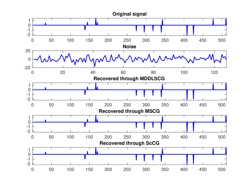
Figure 4: Signal recovery for data $(m,n,k)=(128,512,16)$

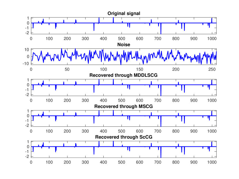
Figure 6: Signal recovery for data $(m,n,k)=(256,1024,32)$

Dimensions $(m,n,k)$	Method	Itr	Tcpu	MSE	RelErr
(128,512,16)	MDDLSCG	272	1.186382e-01	2.033486e-06	7.487872e-03
	MSCG	493	1.606987e-01	2.033495e-06	7.488087e-03
	ScCG	3653	1.135658e+00	2.033588e-06	7.712389e-03
(256,1024,32)	MDDLSCG	291	2.163503e-01	2.128598e-06	9.721181e-03
	MSCG	1405	8.339790e-01	2.128516e-06	9.720993e-03
	ScCG	3002	1.746555e+00	2.229608e-04	9.949161e-02

Table 2: Comparison table for methods MDDLSCG, MSCG and ScCG

6 Conclusions

We presented a modified descent Dai-Liao spectral conjugate gradient (MDDLSCG) method that incorporates a new secant condition and quasi-Newton direction. The updated method introduces spectral parameters ensuring a sufficient descent property independent of line search techniques. Theoretical analysis establishes the global convergence of the method for general nonlinear functions under standard assumptions. Numerical experiments and an application in signal processing demonstrate the improved performance and practical effectiveness of the proposed algorithm, highlighting its potential in optimization and related applications.

References

• \bibcommenthead
• MR [1952] MR, H.: Methods of conjugate gradients for solving linear systems. Journal of Research of the National Bureau of Standards 49(6), 409–436 (1952)
• Fletcher and Reeves [1964] Fletcher, R., Reeves, C.M.: Function minimization by conjugate gradients. The computer journal 7(2), 149–154 (1964)
• Polak and Ribiere [1969] Polak, E., Ribiere, G.: Note sur la convergence de méthodes de directions conjuguées. Revue française d’informatique et de recherche opérationnelle. Série rouge 3(16), 35–43 (1969)
• Dai and Liao [2001] Dai, Y.-H., Liao, L.-Z.: New conjugacy conditions and related nonlinear conjugate gradient methods. Applied Mathematics and optimization 43, 87–101 (2001)
• Fletcher [1987] Fletcher, R.: Practical Methods of Optimization, 2nd edn. A Wiley-Interscience Publication, p. 436. John Wiley & Sons, Ltd., Chichester (1987)
• Dai and Yuan [1999] Dai, Y.-H., Yuan, Y.: A nonlinear conjugate gradient method with a strong global convergence property. SIAM Journal on optimization 10(1), 177–182 (1999)
• Hager and Zhang [2006] Hager, W.W., Zhang, H.: A survey of nonlinear conjugate gradient methods. Pacific journal of Optimization 2(1), 35–58 (2006)
• Hager and Zhang [2005] Hager, W.W., Zhang, H.: A new conjugate gradient method with guaranteed descent and an efficient line search. SIAM Journal on optimization 16(1), 170–192 (2005)
• Dai and Kou [2013] Dai, Y.-H., Kou, C.-X.: A nonlinear conjugate gradient algorithm with an optimal property and an improved wolfe line search. SIAM Journal on Optimization 23(1), 296–320 (2013)
• Shanno [1978] Shanno, D.F.: Conjugate gradient methods with inexact searches. Mathematics of operations research 3(3), 244–256 (1978)
• Babaie-Kafaki and Ghanbari [2014a] Babaie-Kafaki, S., Ghanbari, R.: A descent family of Dai–Liao conjugate gradient methods. Optimization Methods and Software 29(3), 583–591 (2014)
• Babaie-Kafaki and Ghanbari [2014b] Babaie-Kafaki, S., Ghanbari, R.: The Dai–Liao nonlinear conjugate gradient method with optimal parameter choices. European Journal of Operational Research 234(3), 625–630 (2014)
• Babaie-Kafaki [2016] Babaie-Kafaki, S.: On optimality of two adaptive choices for the parameter of Dai–Liao method. Optimization Letters 10, 1789–1797 (2016)
• Barzilai and Borwein [1988] Barzilai, J., Borwein, J.M.: Two-point step size gradient methods. IMA journal of numerical analysis 8(1), 141–148 (1988)
• Raydan [1997] Raydan, M.: The barzilai and borwein gradient method for the large scale unconstrained minimization problem. SIAM Journal on Optimization 7(1), 26–33 (1997)
• Birgin and Martínez [2001] Birgin, E.G., Martínez, J.M.: A spectral conjugate gradient method for unconstrained optimization. Applied Mathematics and optimization 43, 117–128 (2001)
• Yu et al. [2008] Yu, G., Guan, L., Chen, W.: Spectral conjugate gradient methods with sufficient descent property for large-scale unconstrained optimization. Optimization Methods and Software 23(2), 275–293 (2008)
• Perry [1978] Perry, A.: A modified conjugate gradient algorithm. Operations Research 26(6), 1073–1078 (1978)
• Andrei [2007] Andrei, N.: A scaled BFGS preconditioned conjugate gradient algorithm for unconstrained optimization. Applied Mathematics Letters 20(6), 645–650 (2007)
• Andrei [2008] Andrei, N.: Another hybrid conjugate gradient algorithm for unconstrained optimization. Numerical Algorithms 47(2), 143–156 (2008)
• Andrei [2010a] Andrei, N.: Accelerated scaled memoryless BFGS preconditioned conjugate gradient algorithm for unconstrained optimization. European Journal of Operational Research 204(3), 410–420 (2010)
• Andrei [2010b] Andrei, N.: New accelerated conjugate gradient algorithms as a modification of Dai–Yuan’s computational scheme for unconstrained optimization. Journal of computational and applied mathematics 234(12), 3397–3410 (2010)
• Babaie-Kafaki and Mahdavi-Amiri [2013] Babaie-Kafaki, S., Mahdavi-Amiri, N.: Two modified hybrid conjugate gradient methods based on a hybrid secant equation. Mathematical Modelling and Analysis 18(1), 32–52 (2013)
• Li and Fukushima [2001] Li, D.-H., Fukushima, M.: A modified BFGS method and its global convergence in nonconvex minimization. Journal of Computational and Applied Mathematics 129(1-2), 15–35 (2001)
• Zhou and Zhang [2006] Zhou, W., Zhang, L.: A nonlinear conjugate gradient method based on the MBFGS secant condition. Optimisation Methods and Software 21(5), 707–714 (2006)
• Faramarzi and Amini [2019] Faramarzi, P., Amini, K.: A modified spectral conjugate gradient method with global convergence. Journal of Optimization Theory and Applications 182, 667–690 (2019)
• Jian et al. [2017] Jian, J., Chen, Q., Jiang, X., Zeng, Y., Yin, J.: A new spectral conjugate gradient method for large-scale unconstrained optimization. Optimization Methods and Software 32(3), 503–515 (2017)
• Zoutendijk [1970] Zoutendijk, G.: Nonlinear programming, computational methods. Integer and nonlinear programming, 37–86 (1970)
• Mrad and Fakhari [2024] Mrad, H., Fakhari, S.M.: Optimization of unconstrained problems using a developed algorithm of spectral conjugate gradient method calculation. Mathematics and Computers in Simulation 215, 282–290 (2024)
• Bruckstein et al. [2009] Bruckstein, A.M., Donoho, D.L., Elad, M.: From sparse solutions of systems of equations to sparse modeling of signals and images. SIAM review 51(1), 34–81 (2009)
• Aminifard et al. [2022] Aminifard, Z., Hosseini, A., Babaie-Kafaki, S.: Modified conjugate gradient method for solving sparse recovery problem with nonconvex penalty. Signal Processing 193, 108424 (2022)
• Esmaeili et al. [2019] Esmaeili, H., Shabani, S., Kimiaei, M.: A new generalized shrinkage conjugate gradient method for sparse recovery. Calcolo 56, 1–38 (2019)
• Zhu et al. [2013] Zhu, H., Xiao, Y., Wu, S.-Y.: Large sparse signal recovery by conjugate gradient algorithm based on smoothing technique. Computers & Mathematics with Applications 66(1), 24–32 (2013)
• Nesterov [2005] Nesterov, Y.: Excessive gap technique in nonsmooth convex minimization. SIAM Journal on Optimization 16(1), 235–249 (2005)
• Black and Rangarajan [1996] Black, M.J., Rangarajan, A.: On the unification of line processes, outlier rejection, and robust statistics with applications in early vision. International journal of computer vision 19(1), 57–91 (1996)
• Becker et al. [2011] Becker, S., Bobin, J., Candès, E.J.: Nesta: A fast and accurate first-order method for sparse recovery. SIAM Journal on Imaging Sciences 4(1), 1–39 (2011)