Parameter-Robust Preconditioners for A Four-Field Thermo-Poroelasticity Model

Abstract

We study a thermo-poroelasticity model which describes the interaction between the deformation of an elastic porous material and fluid flow under non-isothermal conditions. The model involves several parameters that can vary significantly in practical applications, posing a challenge for developing discretization techniques and solution algorithms that handle such variations effectively. We propose a four-field formulation and apply a conforming finite element discretization. The primary focus is on constructing and analyzing preconditioners for the resulting linear system. Two preconditioners are proposed: one involves regrouping variables and treating the 4-by-4 system as a 2-by-2 block form, while the other is directly constructed from the 4-by-4 coupled operator. Both preconditioners are demonstrated to be robust with respect to variations in parameters and mesh refinement. Numerical experiments are presented to demonstrate the effectiveness of the proposed preconditioners and validate their theoretical performance under varying parameter settings.

65M60, 65F08, 65F10

1 Introduction

In this work, we explore numerical methods for the thermo-poroelasticity model, which describes the coupled interaction between non-isothermal fluid flow and the deformation of porous materials. The model is a coupling of Biot’s equation [33, 5, 6] with the heat equation, specifically addressing the interaction within poroelasticity, encompassing mechanical effects, fluid flow, and heat transfer in porous media. Let $\Omega\subset\mathbb{R}^{d}$ $(d=2,3)$ be an open, bounded domain with a Lipschitz polyhedral boundary $\partial\Omega$, and let $J=(0,t_{f})$ denote the time interval, where $t_{f}>0$ represents the final time. The resulting space-time domain is $\Omega\times J$. The general nonlinear thermo-poroelasticity model [13, 12, 11] is formulated as: finding $(\bm{u},p,T)$ such that

(1.1) $$-\nabla\cdot(2\mu\bm{\varepsilon}(\bm{u})+\lambda\nabla\cdot\bm{u}\bm{I})+\alpha\nabla p+\beta\nabla T =\bm{f},\quad\text{in }\Omega\times J,$$

$$\frac{\partial}{\partial t}(c_{0}p-b_{0}T+\alpha\nabla\cdot\bm{u})-\nabla\cdot(\bm{K}\nabla p) =g,\quad\text{in }\Omega\times J,$$

$$\frac{\partial}{\partial t}(a_{0}T-b_{0}p+\beta\nabla\cdot\bm{u})-C_{f}(\bm{K}\nabla p)\cdot\nabla T-\nabla\cdot(\bm{\Theta}\nabla T) =h,\quad\text{in }\Omega\times J.$$

Here, the operator $\bm{\varepsilon}$ is defined as $\bm{\varepsilon}(\bm{u})=\frac{1}{2}(\nabla\bm{u}+\nabla\bm{u}^{T})$ and $\bm{I}$ is the identity tensor. The variables $\bm{u}$, $p$, and $T$ represent the displacement, fluid pressure, and temperature distribution, respectively. The right-hand side terms $\bm{f}$, $g$, and $h$ correspond to the body force, mass source, and heat source, respectively. The three equations in (1.1) reflect the principles of momentum conservation, mass conservation, and energy conservation. For a comprehensive derivation of the model, readers are referred to [13], which incorporates an additional nonlinear convective term involving $\frac{\partial}{\partial t}\bm{u}$ and $\nabla T$. However, as indicated in [11, 12, 34], this term is considered negligible in comparison to the heat convection term associated with the Darcy velocity. The parameters $\bm{K}=(K_{ij})^{d}_{ij=1}$ and $\bm{\Theta}=(\Theta_{ij})^{d}_{ij=1}$ are matrices determined by the medium’s permeability and the fluid viscosity. Detailed descriptions of other parameters, including their physical meanings and corresponding units, can be found in Table 1, where the problem parameters for (1.1) are summarized. Additionally, the bulk modulus of the porous material, $K_{D}$, is related to the two Lamé parameters $\lambda$ and $\mu$ by the formula $K_{D}:=d^{-1}(d\lambda+2\mu)$. For further discussion on parameter relations, we refer to [1].

In the following, the system (1.1) is completed by boundary conditions

(1.2) $$\bm{u}=\bm{0},~p=0,\text{ and }T=0,\text{ on }\partial\Omega\times J,$$

and initial conditions

(1.3) $$\bm{u}(\cdot,0)=\bm{u}^{0},~p(\cdot,0)=p^{0},~T(\cdot,0)=T^{0},\text{ in }\Omega\times\{0\},$$

for some known functions $\bm{u}^{0},p^{0}$ and $T^{0}$.

Table 1: Thermo-Poroelasticity Model Parameters and Their Units

Notation	Quantity	Unit
$a_{0}$	thermal capacity	$Pa/K^{2}$
$b_{0}$	thermal dilatation coefficient	$K^{-1}$
$c_{0}$	specific storage coefficient	$Pa^{-1}$
$\alpha$	Biot-Willis constant	-
$\beta$	thermal stress coefficient	$Pa/K$
$C_{f}$	fluid volumetric heat capacity divided	$Pa/K^{2}$
	by reference temperature
$\mu,\lambda$	Lamé coefficients	$Pa$
$\bm{K}$	permeability divided by fluid viscosity	$m^{2}/(Pas)$
$\bm{\Theta}$	effective thermal conductivity	$m^{2}Pa/(K^{2}s)$

Recent advancements in numerical analysis for thermo-poroelasticity models include studies on solution existence, uniqueness, and energy estimates for nonlinear problems, as in [12]. Transforming the three-field model into a four-field formulation has enabled the development of multiphysics finite element methods for both linear and nonlinear cases, including convective transport terms [16, 18]. Mixed finite element and hybrid techniques have been applied to these models [16, 37, 38]. Robust discontinuous Galerkin methods for fully coupled nonlinear models are detailed in [7, 1]. Iterative coupling techniques include sequential iteration methods for linear problems [25] and splitting schemes for decoupling poroelasticity and thermoelasticity [26]. A five-field formulation incorporating heat and Darcy fluxes is presented in [11], with both monolithic and decoupled schemes. Recently, reduced-order modeling was introduced in [3] to enhance the efficiency of decoupled iterative solutions.

Numerical solutions for the thermo-poroelasticity model are challenging, partly due to significant variations in model parameters across applications. For example, in macroscopic thermo-poroelasticity models within rock mechanics [34], permeability can vary drastically, ranging from $10^{-5}$ to $10^{-20}$ $m^{2}$. Similarly, in non-isothermal fluid flow models through deformable porous media [35], the Lamé coefficients are on the order of $O(1)$ in magnitude, implying that the bulk modulus is also $O(1)$ in $Pa$, while permeability is around $O(10^{-4})$ $m^{2}$. In contrast, models that involve rigid one-dimensional fluid cavities [32] exhibit bulk moduli on the order of $GPa$, with permeability varying around $O(10^{-19})$ $m^{2}$. Additionally, spatial and temporal discretizations introduce discretization parameters, further complicating the problem. Effective numerical methods must therefore remain robust against significant variations in both model and discretization parameters. For example, [23, 27, 31, 8] developed parameter-robust finite element discretizations and uniform block-diagonal preconditioners for poroelasticity models. However, the challenges of ensuring parameter robustness and effective preconditioning for thermo-poroelasticity models remain unaddressed. For large discrete systems solved via iterative methods, the convergence rate heavily depends on the condition numbers of preconditioned systems [2, 21]. Although preconditioning techniques for poroelasticity have been studied in [27, 23, 14], no effort has focused on thermo-poroelasticity models.

This paper addresses a key gap by proposing a stable finite element method for the thermo-poroelasticity model and developing the corresponding preconditioners. The primary aim is to ensure that the condition number of the preconditioned systems remains bounded across a wide range of model parameters. To focus on the preconditioner design, we omit nonlinear terms. Similar to the quasi-static Biot’s model, Poisson locking [30, 27] occurs when the Lamé constant $\lambda$ approaches infinity. To address this, we introduce an auxiliary variable, $\xi=-\lambda\nabla\cdot\bm{u}+\alpha p+\beta T$, which captures the volumetric contribution to the total stress. This reformulation transforms the original three-field formulation into a symmetric four-field model, effectively mitigating Poisson locking and enabling the application of the operator preconditioning framework from [29, 24]. Upon discretization, the four-field formulation results in a large, indefinite linear system. To address this, we analyze the system’s stability within weighted Hilbert spaces and apply operator preconditioning techniques. By defining appropriate norms, we prove that the constants in the boundedness and inf-sup conditions are independent of the model parameters, ensuring the framework’s uniform robustness under minimal assumptions. To validate the effectiveness of the proposed preconditioners, we conduct numerical experiments using both exact LU decomposition and inexact algebraic multigrid (AMG) solver for the elliptic operators. These experiments demonstrate the preconditioners’ robustness with respect to both the physical parameters of the model and the discretization parameters.

The paper is structured as follows. Section 2 presents a linear thermo-poroelastic model and its four-field reformulation, leading to a symmetric indefinite linear system after time discretization. Section 3 introduces two preconditioners and examines their robustness with respect to physical parameters. Section 4 details the construction of a conforming finite element discretization and parameter-robust preconditioners. Section 5 provides numerical experiments to validate the theoretical findings.

2 Parameter-dependent systems

Throughout this paper, we adopt the following definitions and notations. Let $L^{p}(\Omega)$ denote the standard Lebesgue space on $\Omega$ with index $p\in[1,\infty]$. In particular, for $p=2$, $L^{2}(\Omega)$ represents the space of square-integrable functions on $\Omega$, equipped with the inner product $(\cdot,\cdot)$ and norm $\|\cdot\|_{0}$. For Sobolev spaces, we define $W^{m,p}(\Omega)=\{u\,|\,D^{\alpha}u\in L^{p}(\Omega),0\leq\alpha\leq m,\|u\|_{W^{m,p}}<\infty\}$, and write $H^{m}(\Omega)$ as shorthand for $W^{m,2}(\Omega)$, with $\|\cdot\|_{H^{m}(\Omega)}$ representing the associated norm. We denote $H^{m}_{0}(\Omega)$ as the subspace of $H^{m}(\Omega)$ with a vanishing trace on $\partial\Omega$, and $H^{m}_{0,\Gamma}(\Omega)$ as the subspace of $H^{m}(\Omega)$ with a vanishing trace on $\Gamma\subset\partial\Omega$. Specifically, for $m=2$, we use $\|\cdot\|_{1}$ in place of $\|\cdot\|_{H^{m}(\Omega)}$ or $\|\cdot\|_{W^{m,2}(\Omega)}$. For a Banach space $X$, we define $L^{p}(J;X)=\{v\,|\,(\int_{J}\|v\|_{X}^{p})^{\frac{1}{p}}<\infty\}$ and $H^{1}(J;X)=\{v\,|\,(\int_{J}(\|v\|_{0}^{2}+\|\partial_{t}v\|_{0}^{2})\,dt)^{\frac{1}{2}}<\infty\}$.

2.1 A simplified linear thermo-poroelastic model

As stated earlier, the nonlinear term $C_{f}(\bm{K}\nabla p)\cdot\nabla T$ in (1.1) is omitted to simplify the discussion. Therefore, we focus on the following simplified linear thermo-poroelastic model.

(2.1) $$-\nabla\cdot(2\mu\bm{\varepsilon}(\bm{u})+\lambda\nabla\cdot\bm{u}\bm{I})+\alpha\nabla p+\beta\nabla T =\bm{f},\quad\text{in }\Omega\times J,$$

$$\frac{\partial}{\partial t}(c_{0}p-b_{0}T+\alpha\nabla\cdot\bm{u})-\nabla\cdot(\bm{K}\nabla p) =g,\quad\text{in }\Omega\times J,$$

$$\frac{\partial}{\partial t}(a_{0}T-b_{0}p+\beta\nabla\cdot\bm{u})-\nabla\cdot(\bm{\Theta}\nabla T) =h,\quad\text{in }\Omega\times J.$$

We retain the Dirichlet boundary conditions (1.2) and the initial condition (1.3). In practical scenarios, nonhomogeneous Dirichlet and Neumann boundary conditions are commonly encountered. The analysis performed for homogeneous boundary conditions can be straightforwardly extended to accommodate these cases. We assume that $g,h\in L^{2}(J;L^{2}(\Omega))$ and $\bm{f}\in[H^{1}(J;L^{2}(\Omega))]^{d}$. And we assume that the initial conditions satisfy $p^{0},T^{0}\in H_{0}^{1}(\Omega)$ and $\bm{u}^{0}\in[H_{0}^{1}(\Omega)]^{d}$. Furthermore, as outlined in [11], we adopt the following assumptions for the model parameters throughout this paper (similar assumptions are also discussed in [16, 38]):

(A1) Assume that $\bm{K}=K\bm{I}$ and $\bm{\Theta}=\theta\bm{I}$, where $K$ and $\theta$ are positive constants bounded both above and below, and $\bm{I}$ denotes the identity matrix.

(A2) The constants $a_{0},b_{0},c_{0},\alpha$, $\beta$, $\lambda$ and $\mu$ are strictly positive constants.

(A3) The coefficients $a_{0}$, $b_{0}$, and $c_{0}$ are constants satisfying $c_{0}-b_{0}>0$ and $a_{0}-b_{0}>0$.

For convenience, we introduce the following parameter transformations:

$$t_{K}=\Delta tK,~t_{\theta}=\Delta t\theta,~c_{\alpha}=\left(c_{0}+\frac{\alpha^{2}}{\lambda}\right),~c_{\alpha\beta}=\left(\frac{\alpha\beta}{\lambda}-b_{0}\right),~c_{\beta}=\left(a_{0}+\frac{\beta^{2}}{\lambda}\right).$$

Additionally, to further simplify, we assume $2\mu=1$.

We now introduce the four-field formulation for the linear component of (2.1). More clearly, following the methodology for handling Biot’s problem in [27, 30], we define an auxiliary variable to represent the volumetric contribution to the total stress:

$$\xi=-\lambda\nabla\cdot\bm{u}+\alpha p+\beta T,$$

which is commonly referred to as the pseudo-total pressure [1]. Substituting this variable into equation (2.1) and using parameter transformations above, the four-field thermo-poroelasticity problem can be expressed as:

(2.2) $$-\nabla\cdot\bm{\varepsilon}(\bm{u})+\nabla\xi =\bm{f},$$

$$-\lambda\nabla\cdot\bm{u}-\xi+\alpha p+\beta T =0,$$

$$\frac{\partial}{\partial t}(-\frac{\alpha}{\lambda}\xi+c_{\alpha}p+c_{\alpha\beta}T)-\nabla\cdot(K\nabla p) =g,$$

$$\frac{\partial}{\partial t}(-\frac{\beta}{\lambda}\xi+c_{\alpha\beta}p+c_{\beta}T)-\nabla\cdot(\theta\nabla T) =h.$$

For the time discretization, we use an equidistant partition of the interval $[0,t_{f}]$ with a constant step size $\Delta t$. At any time step, the relationship is given by $t_{n}=t_{n-1}+\Delta t$. Using the backward Euler method, we solve for $(\bm{u}^{n},\xi^{n},p^{n},T^{n})$ at each time step based on the equation (2.3), as follows:

(2.3) $$-\nabla\cdot\bm{\varepsilon}(\bm{u}^{n})+\nabla\xi^{n} =\bm{f}^{n},$$

$$-\lambda\nabla\cdot\bm{u}^{n}-\xi^{n}+\alpha p^{n}+\beta T^{n} =0,$$

$$-\frac{\alpha}{\lambda}\xi^{n}+c_{\alpha}p^{n}-\Delta t\nabla\cdot(K\nabla p^{n})+c_{\alpha\beta}T^{n} =\tilde{g}^{n},$$

$$-\frac{\beta}{\lambda}\xi^{n}+c_{\alpha\beta}p^{n}+c_{\beta}T^{n}-\Delta t\nabla\cdot(\theta\nabla T^{n}) =\tilde{h}^{n},$$

where

$$\bm{u}^{n}=\bm{u}(\bm{x};t_{n}),~\xi^{n}=\xi(\bm{x};t_{n}),~p^{n}=p(\bm{x};t_{n}),~\bm{f}^{n}=\bm{f}(\bm{x};t_{n}),$$

$$\tilde{g}^{n}=\Delta tg(\bm{x};t_{n})-\frac{\alpha}{\lambda}\xi(\bm{x};t_{n-1})+c_{\alpha}p(\bm{x};t_{n-1})+c_{\alpha\beta}T(\bm{x};t_{n-1}),$$

and

$$\tilde{h}^{n}=\Delta th(\bm{x};t_{n})-\frac{\beta}{\lambda}\xi(\bm{x};t_{n-1})+c_{\alpha\beta}p(\bm{x};t_{n-1})+c_{\beta}T(\bm{x};t_{n-1}).$$

Since our focus is on the system of linear equations at a specific time step $n$, we simplify the notation by omitting the time-step subscript. Thus, we replace $\bm{u}^{n},\xi^{n},p^{n},T^{n},\bm{f}^{n},\tilde{g}^{n}$, and $\tilde{h}^{n}$ with $\bm{u},\xi,p,T,\bm{f},\tilde{g}$, and $\tilde{h}$, respectively. This results in the following system of equations:

(2.4) $$-\nabla\cdot\bm{\varepsilon}(\bm{u})+\nabla\xi =\bm{f},$$

$$-\nabla\cdot\bm{u}-\lambda^{-1}\xi+\frac{\alpha}{\lambda}p+\frac{\beta}{\lambda}T =0,$$

$$\frac{\alpha}{\lambda}\xi-c_{\alpha}p+t_{K}\nabla\cdot(\nabla p)-c_{\alpha\beta}T =-\tilde{g},$$

$$\frac{\beta}{\lambda}\xi-c_{\alpha\beta}p-c_{\beta}T+t_{\theta}\nabla\cdot(\nabla T) =-\tilde{h}.$$

We define the following functional spaces:

$$\bm{V}=[H^{1}_{0}(\Omega)]^{d},\quad Q=L^{2}(\Omega),\quad W=H_{0}^{1}(\Omega).$$

The corresponding continuous variational formulation for (2.4) is stated as follows: find $(\bm{u},\xi,p,T)\in\bm{V}\times Q\times W\times W$ such that, for all $(\bm{v},\phi,q,S)\in\bm{V}\times Q\times W\times W$, the following holds:

(2.5) $$(\bm{\varepsilon}(\bm{u}),\bm{\varepsilon}(\bm{v}))-(\nabla\cdot\bm{v},\xi) =(\bm{f},\bm{v}),$$

$$-(\nabla\cdot\bm{u},\phi)-({\lambda^{-1}}\xi,\phi)+(\frac{\alpha}{\lambda}p,\phi)+(\frac{\beta}{\lambda}T,\phi) =0,$$

$$(\frac{\alpha}{\lambda}\xi,q)-(c_{\alpha}p,q)-(t_{K}\nabla p,\nabla q)-(c_{\alpha\beta}T,q) =(-\tilde{g},q),$$

$$(\frac{\beta}{\lambda}\xi,S)-(c_{\alpha\beta}p,S)-(c_{\beta}T,S)-(t_{\theta}\nabla T,\nabla S) =(-\tilde{h},S).$$

3 Preconditioners and parameter-robust stability

Let $X$ be a separable, real Hilbert space equipped with a norm $\|\cdot\|_{X}$, to be defined later, and let its dual space be denoted by $X^{*}$. Consider an operator $\mathcal{A}:X\to X^{*}$, which is an invertible, symmetric isomorphism and belongs to the space of bounded linear operators, $\mathcal{L}(X,X^{*})$. Given $\mathcal{F}\in X^{*}$, the goal is to find $x\in X$ such that:

$$\mathcal{A}x=\mathcal{F}.$$

The operator norm of $\mathcal{A}$ in $\mathcal{L}(X,X^{*})$ is defined as:

$$\|\mathcal{A}\|_{\mathcal{L}(X,X^{*})}=\sup_{x\in X}\frac{\|\mathcal{A}x\|_{X^{*}}}{\|x\|_{X}}.$$

To improve computational efficiency, a preconditioner $\mathcal{B}^{-1}\in\mathcal{L}(X^{*},X)$, which is a symmetric isomorphism, is introduced. The preconditioned problem is written as:

$$\mathcal{B}^{-1}\mathcal{A}x=\mathcal{B}^{-1}\mathcal{F}.$$

The convergence rate of iterative methods, such as the MinRes method for solving this problem depends on the condition number $\kappa(\mathcal{B}^{-1}\mathcal{A})$, defined as:

$$\kappa(\mathcal{B}^{-1}\mathcal{A})=\|\mathcal{B}^{-1}\mathcal{A}\|_{\mathcal{L}(X,X)}\|(\mathcal{B}^{-1}\mathcal{A})^{-1}\|_{\mathcal{L}(X,X)}.$$

For a parameter-dependent operator $\mathcal{A}_{\epsilon}\in\mathcal{L}(X_{\epsilon},X^{*}_{\epsilon})$, the objective is to design a preconditioner $\mathcal{B}_{\epsilon}$ such that the condition number of the preconditioned system is robust with respect to a set of parameters $\epsilon$ (including $\mu$, $\lambda$, $\alpha$, $\beta$, $a_{0}$, $b_{0}$, $c_{0}$, $K$, and $\theta$). We assume that appropriate function spaces $X_{\epsilon}$ and $X_{\epsilon}^{*}$ can be identified such that the following operator norms:

$$\|\mathcal{A}_{\epsilon}\|_{\mathcal{L}(X_{\epsilon},X_{\epsilon}^{*})},\quad\|(\mathcal{A}_{\epsilon})^{-1}\|_{\mathcal{L}(X_{\epsilon}^{*},X_{\epsilon})},\quad\|\mathcal{B}_{\epsilon}\|_{\mathcal{L}(X_{\epsilon}^{*},X_{\epsilon})},\quad\|(\mathcal{B}_{\epsilon})^{-1}\|_{\mathcal{L}(X_{\epsilon},X_{\epsilon}^{*})}$$

remain uniformly bounded, independent of the parameters $\epsilon$. Under these assumptions, the condition number $\kappa(\mathcal{B}_{\epsilon}^{-1}\mathcal{A}_{\epsilon})$ will also be uniformly bounded, regardless of the values of $\epsilon$.

We note that the system (2.4) can be expressed in operator form as follows:

(3.1) $$\begin{bmatrix}-\text{div }\bm{\varepsilon}&\nabla&0&0\\ -\text{div}&-\lambda^{-1}I&\frac{\alpha}{\lambda}I&\frac{\beta}{\lambda}I\\ 0&\frac{\alpha}{\lambda}I&-c_{\alpha}I+t_{K}\text{div}(\nabla)&-c_{\alpha\beta}I\\ 0&\frac{\beta}{\lambda}I&-c_{\alpha\beta}I&-c_{\beta}I+t_{\theta}\text{div}(\nabla)\\ \end{bmatrix}\begin{bmatrix}\bm{u}\\ \xi\\ p\\ T\end{bmatrix}=\begin{bmatrix}\bm{f}\\ 0\\ -\tilde{g}\\ -\tilde{h}\end{bmatrix},$$

where $I$ is an identity operator. Let the coefficient matrix of the system be denoted by the operator $\mathcal{A}$ and the right-hand side part be denoted by $\mathcal{F}$. For simplicity, we rewrite the system (3.1) as:

$$\mathcal{A}(\bm{u},\xi,p,T)=\mathcal{F}.$$

It is easy to test that $\mathcal{A}$ is a symmetric linear operator with respect to the Dirichlet boundary condition:

$$(\mathcal{A}(\bm{u},\xi,p,T),(\bm{v},\phi,q,S)) =((\bm{u},\xi,p,T),\mathcal{A}(\bm{v},\phi,q,S))$$

$$=(\bm{\varepsilon}(\bm{u}),\bm{\varepsilon}(\bm{v}))-(\nabla\cdot\bm{v},\xi)-(\nabla\cdot\bm{u},\phi)-({\lambda^{-1}}\xi,\phi)$$

$$+(\frac{\alpha}{\lambda}p,\phi)+(\frac{\beta}{\lambda}T,\phi)+(\frac{\alpha}{\lambda}\xi,q)-(c_{\alpha}p,q)-(t_{K}\nabla p,\nabla q)$$

$$-(c_{\alpha\beta}T,q)+(\frac{\beta}{\lambda}\xi,S)-(c_{\alpha\beta}p,S)-(c_{\beta}T,S)-(t_{\theta}\nabla T,\nabla S).$$

Before we define appropriate parameter-dependent norms for $\mathcal{A}$, we first recall the Lamé problem in linear elasticity: Find $\bm{u}:\Omega\rightarrow\mathbb{R}^{d}$, $p:\Omega\rightarrow\mathbb{R}$ for

(3.2) $$-\text{div}(\bm{\varepsilon}(\bm{u}))+\nabla p=\bm{f},$$

$$-\text{div}\bm{u}-\frac{1}{\lambda}p=g,$$

with $\bm{u}|_{\partial\Omega}=\bm{0}$. Here, $1\leq\lambda<+\infty$ is a positive constant and $\bm{\varepsilon}(\bm{u})$ is the symmetric gradient of $\bm{u}$. When the three variables $(\xi,p,T)$ are grouped together, the system in (3.1) resembles the problem in (3.2). The variational form of problem (3.2) reads as: find $\bm{u}\in[H_{0}^{1}(\Omega)]^{d}$ and $p\in L^{2}(\Omega)$ such that:

(3.3) $$(\bm{\varepsilon}(\bm{u}),\bm{\varepsilon}(\bm{v}))-(p,\text{div}\bm{v})=(f,\bm{v}),\quad\forall\bm{v}\in[H_{0}^{1}(\Omega)]^{d},$$

$$-(\text{div}\bm{u},q)-\frac{1}{\lambda}(p,q)=(g,q),\quad\forall q\in L^{2}(\Omega).$$

In this saddle point problem, the stabilizing term $\frac{1}{\lambda}(p,q)$ weakens as $\lambda$ increases. In the limiting case where $\lambda=+\infty$, the system becomes unstable under standard norms such as $(\|\bm{u}\|_{1}^{2}+\|p\|_{0}^{2})^{1/2}$. This instability arises because $\text{div}[H_{0}^{1}(\Omega)]^{d}\subsetneq L^{2}(\Omega)$. To ensure $\lambda$-independent stability for the system, it is important to note that $\text{div}[H_{0}^{1}(\Omega)]^{d}$ controls only the $L^{2}(\Omega)$ norm of the zero-mean component of $p$, leaving the mean value part of $p$ uncontrolled without the stabilizing term. For any $\phi\in L^{2}(\Omega)$, its mean-value and mean-zero components are defined as

(3.4) $$\phi_{m}:=P_{m}\phi\quad\text{and}\quad\phi_{0}:=\phi-\phi_{m},$$

where

$$P_{m}\phi:=\left(\frac{1}{|\Omega|}\int_{\Omega}\phi\,dx\right)\chi_{\Omega},$$

with $\chi_{\Omega}$ representing the characteristic function of $\Omega$, and $|\Omega|$ denoting the Lebesgue measure of $\Omega$. To achieve $\lambda$-robust stability for the problem in (3.3), the appropriate Hilbert space with a $\lambda$-independent norm is given by:

$$\|(\bm{u},p)\|^{2}=\|\bm{u}\|_{1}^{2}+\frac{1}{\lambda}\|p_{m}\|_{0}^{2}+\|p_{0}\|_{0}^{2}.$$

Such a formulation naturally suggests considering $p\in\lambda^{-1/2}L^{2}(\Omega)\cap L_{0}^{2}(\Omega)$. This leads to a $\lambda$-robust preconditioner for the problem (3.2) as proposed in [27]:

(3.5) $$\begin{bmatrix}-\Delta^{-1}&0\\ 0&(\frac{1}{\lambda}I_{m}+I_{0})^{-1}\end{bmatrix}.$$

Here, $I_{0}$ represents the Riesz map from $L^{2}(\Omega)$ to the dual of $L^{2}_{0}(\Omega)$, while $I_{m}$ is the corresponding operator mapping $L^{2}(\Omega)$ to the dual of the complement of $L^{2}_{0}(\Omega)$.

3.1 A parameter-robust preconditioner by regrouping variables

By grouping the variables into $\bm{u}$ and $(\xi,p,T)$, and utilizing the product space $\bm{V}\times(Q\times W\times W)$, the system (3.1) can be reformulated into the standard saddle point structure:

(3.6) $$\mathcal{A}=\begin{bmatrix}A_{0}&B_{0}^{*}\\ B_{0}&-C_{0}\end{bmatrix},$$

where $A_{0}=-\text{div}\bm{\varepsilon},B_{0}=(-\text{div},0,0)^{T},$ and

$$C_{0}=\begin{bmatrix}&\lambda^{-1}I&-\frac{\alpha}{\lambda}I&-\frac{\beta}{\lambda}I\\ &-\frac{\alpha}{\lambda}I&c_{\alpha}I-t_{K}\text{div}(\nabla)&c_{\alpha\beta}I\\ &-\frac{\beta}{\lambda}I&c_{\alpha\beta}I&c_{\beta}I-t_{\theta}\text{div}(\nabla)\end{bmatrix},$$

and $B_{0}^{*}=(\nabla,0,0)$ is the adjoint operator of $B_{0}$. Building on the parameter-robust preconditioner developed for saddle point problems with a penalty term, as detailed in [8, 9, 24], and leveraging the block-processing method for multi-network poroelasticity problems from [31], we adapt and extend these methodologies to tackle the thermo-poroelasticity problem presented in this paper.

It is natural to use the block diagonal operator

$$\begin{bmatrix}A_{0}^{-1}&0\\ 0&(C_{0}+B_{0}A_{0}^{-1}B_{0}^{*})^{-1}\end{bmatrix},$$

or its approximation to construct block preconditioners for $\mathcal{A}$. To this end, we consider a parameter-dependent norm for the thermo-poroelasticity problem as follows:

(3.7) $$\|(\bm{u},\xi,p,T)\|_{\mathcal{B}_{1}}^{2}= \|\bm{\varepsilon}(\bm{u})\|_{0}^{2}+\frac{1}{\lambda}\|\xi\|_{0}^{2}+\|\xi_{0}\|_{0}^{2}-2(\frac{\alpha}{\lambda}p,\xi)-2(\frac{\beta}{\lambda}T,\xi)$$

$$+c_{\alpha}\|p\|_{0}^{2}+t_{K}\|\nabla p\|_{0}^{2}+c_{\beta}\|T\|_{0}^{2}+t_{\theta}\|\nabla T\|_{0}^{2}+2(c_{\alpha\beta}p,T),$$

where $\xi_{0}$ is the mean value zero of $\xi$, as defined in (3.4).

The norm defined in (3.7) contains some negative terms, requiring a demonstration to confirm that it qualifies as a valid norm. To address this, we introduce a bilinear form $(\mathcal{B}_{1}\cdot,\cdot)$, where the operator $\mathcal{B}_{1}$ is defined as:

(3.8) $$\mathcal{B}_{1}=\begin{bmatrix}-\text{div }\bm{\varepsilon}&0&0&0\\ 0&\lambda^{-1}I+I_{0}&-\frac{\alpha}{\lambda}I&-\frac{\beta}{\lambda}I\\ 0&-\frac{\alpha}{\lambda}I&c_{\alpha}I-t_{K}\text{div}(\nabla)&c_{\alpha\beta}I\\ 0&-\frac{\beta}{\lambda}I&c_{\alpha\beta}I&c_{\beta}I-t_{\theta}\text{div}(\nabla)\end{bmatrix},$$

and is subject to the same boundary conditions as those in (1.2). We recall that $I$ represents the Riesz map from $Q$ to its dual $Q^{*}$ and $I_{0}$ maps $Q$ to the dual of $Q\cap L_{0}^{2}(\Omega)$. It should be noted that, unlike the preconditioner (3.5) used for the Lamé problem, the preconditioner in (3.9) employs the operator $\lambda^{-1}I+I_{0}$ in the $(2,2)$ block instead of $\lambda^{-1}I_{m}+I_{0}$. For $\lambda\geq 1$, however, these two operators are spectrally equivalent [27]. For further implementation details, we refer the readers to [27, 29]. Additionally, we highlight that the lower $3\times 3$ block of $\mathcal{B}_{1}$ is connected to the preconditioner used in the multiple-network poroelastic model [31], where diagonalization by congruence was applied in order simplify evaluation of the discrete preconditioner in terms of multilevel methods. In contrast, our approach deals directly with the $3\times 3$ operator. In particular, we show in Remark 5.4 that the block is amenable to algebraic multigrid.

Defining an operator matrix $\mathcal{B}_{22}=\begin{bmatrix}0&0&0&0\\ 0&I_{0}&0&0\\ 0&0&0&0\\ 0&0&0&0\end{bmatrix}$and we can split $\mathcal{B}_{1}$ as

$$\mathcal{B}_{1}=\tilde{\mathcal{B}_{1}}+\mathcal{B}_{22},$$

where $\tilde{\mathcal{B}_{1}}=\mathcal{B}_{1}-\mathcal{B}_{22}$. Given the assumption $c_{0}-b_{0}>0$ and $a_{0}-b_{0}>0$, we establish:

$$(c_{0}p,p)+(a_{0}T,T)-2(b_{0}p,T) \geq(c_{0}p,p)+(a_{0}T,T)-(b_{0}p,p)-(b_{0}T,T)$$

$$=(C_{p}p,p)+(C_{T}T,T)>0,$$

for any $(p,T)\neq(0,0)$, where $C_{p}=c_{0}-b_{0}$ and $C_{T}=a_{0}-b_{0}$. Using the definitions of $c_{\alpha}$, $c_{\beta}$, and $c_{\alpha\beta}$, along with Green’s formula and the boundary conditions in (1.2), we derive:

$$(\tilde{\mathcal{B}_{1}}(\bm{u},\xi,p,T),(\bm{u},\xi,p,T))$$

$$= \|\bm{\varepsilon}(\bm{u})\|_{0}^{2}+\left(\frac{1}{\lambda}\xi,\xi\right)-2\left(\frac{\alpha}{\lambda}p,\xi\right)-2\left(\frac{\beta}{\lambda}T,\xi\right)+(c_{\alpha}p,p)+(c_{\beta}T,T)+2(c_{\alpha\beta}p,T)$$

$$+t_{K}\|\nabla p\|_{0}^{2}+t_{\theta}\|\nabla T\|_{0}^{2}$$

$$= \|\bm{\varepsilon}(\bm{u})\|_{0}^{2}+\left(\frac{1}{\lambda}\xi,\xi\right)-2\left(\frac{\alpha}{\lambda}p,\xi\right)-2\left(\frac{\beta}{\lambda}T,\xi\right)+\left(\frac{\alpha^{2}}{\lambda}p,p\right)+\left(\frac{\beta^{2}}{\lambda}T,T\right)$$

$$+2\left(\frac{\alpha\beta}{\lambda}p,T\right)+(c_{0}p,p)+(a_{0}T,T)-2(b_{0}p,T)+t_{K}\|\nabla p\|_{0}^{2}+t_{\theta}\|\nabla T\|_{0}^{2}$$

$$= \|\bm{\varepsilon}(\bm{u})\|_{0}^{2}+\left(-\frac{1}{\sqrt{\lambda}}\xi+\frac{\alpha}{\sqrt{\lambda}}p+\frac{\beta}{\sqrt{\lambda}}T,-\frac{1}{\sqrt{\lambda}}\xi+\frac{\alpha}{\sqrt{\lambda}}p+\frac{\beta}{\sqrt{\lambda}}T\right)$$

$$+(c_{0}p,p)+(a_{0}T,T)-2(b_{0}p,T)+t_{K}\|\nabla p\|_{0}^{2}+t_{\theta}\|\nabla T\|_{0}^{2}$$

$$\geq 0.$$

with equality holding only if $(\bm{u},\xi,p,T)=(\bm{0},0,0,0)$. This demonstrates that $\tilde{\mathcal{B}_{1}}$ is a symmetric positive definite operator, making $(\tilde{\mathcal{B}_{1}}\cdot,\cdot)$ an inner product. Consequently, the quantity

$$\|(\bm{u},\xi,p,T)\|_{\mathcal{B}_{1}}=\Big{(}(\tilde{\mathcal{B}_{1}}(\bm{u},\xi,p,T),(\bm{u},\xi,p,T))+\|\xi_{0}\|_{0}^{2}\Big{)}^{\frac{1}{2}}$$

is a valid norm induced by this inner product. Furthermore, $\mathcal{B}_{1}$ is a bounded linear operator, confirming that the expression in (3.7) defines a proper norm.

The corresponding preconditioner for the continuous system associated with the norm (3.7) can be expressed as:

(3.9) $$\mathcal{B}_{1}^{-1}=\begin{bmatrix}-\text{div }\bm{\varepsilon}&0&0&0\\ 0&\lambda^{-1}I+I_{0}&-\frac{\alpha}{\lambda}I&-\frac{\beta}{\lambda}I\\ 0&-\frac{\alpha}{\lambda}I&c_{\alpha}I-t_{K}\text{div}(\nabla)&c_{\alpha\beta}I\\ 0&-\frac{\beta}{\lambda}I&c_{\alpha\beta}I&c_{\beta}I-t_{\theta}\text{div}(\nabla)\end{bmatrix}^{-1}.$$

We first introduce a lemma that will be used in the following part of the paper to clarify the relationship between $\|\cdot\|_{1}$ and $\|\bm{\varepsilon}(\cdot)\|_{0}$.

Lemma 3.1.

There exists a constant $C_{K}$ such that the Korn’s inequality

$$C_{K}\|\bm{u}\|_{1}^{2}\leq\|\bm{\varepsilon}(\bm{u})\|_{0}^{2},\quad\forall\bm{u}\in[H^{1}_{0}(\Omega)]^{d},d=2,3.$$

holds true [10].

Lemma 3.2 (continuity).

Assume that the conditions (A1)-(A3) are satisfied. Let $X=\bm{V}\times Q\times W\times W$ denote the Hilbert space equipped with the norm defined in (3.7). Let $\mathcal{A}$ represent the operator defined in (3.1). Then, there exists a constant $C$, independent of any problem parameters, such that:

(3.10) $$(\mathcal{A}(\bm{u},\xi,p,T),(\bm{v},\phi,q,S))\leq C\|(\bm{u},\xi,p,T)\|_{\mathcal{B}_{1}}\|(\bm{v},\phi,q,S)\|_{\mathcal{B}_{1}}$$

for all $(\bm{u},\xi,p,T),(\bm{v},\phi,q,S)\in X$.

Proof 3.3.

By the block form of $\mathcal{A}$ in (3.6), we have

(3.11) $$(\mathcal{A}(\bm{u},\xi,p,T),(\bm{v},\phi,q,S))$$

$$= (\begin{bmatrix}A_{0}&B_{0}^{*}\\ B_{0}&-C_{0}\end{bmatrix}(\bm{u},(\xi,p,T)),(\bm{v},(\phi,q,S)))$$

$$= (A_{0}\bm{u},\bm{v})+(B_{0}\bm{u},(\phi,q,S))+(B_{0}^{*}(\xi,p,T),\bm{v})+(-C_{0}(\xi,p,T),(\phi,q,S)).$$

Given that $\bm{u}$ and $\bm{v}$ have vanishing traces, using Green’s formula, the Cauchy-Schwarz inequality, and the definition of the mean-zero value parts in (3.4), we have

(3.12) $$(A_{0}\bm{u},\bm{v})=(\bm{\varepsilon}(\bm{u}),\bm{\varepsilon}(\bm{v}))\leq\|(\bm{u},\xi,p,T)\|_{\mathcal{B}_{1}}\|(\bm{v},\phi,q,S)\|_{\mathcal{B}_{1}},$$

(3.13) $$(B_{0}\bm{u},(\phi,q,S))= -(\nabla\cdot\bm{u},\phi)=-(\nabla\cdot\bm{u},\phi_{0})-(\nabla\cdot\bm{u},\phi_{m})$$

$$\leq \|\nabla\cdot\bm{u}\|_{0}\|\phi_{0}\|_{0}-\phi_{m}\int_{\Omega}\nabla\cdot\bm{u}$$

$$\leq \|\bm{\varepsilon}(\bm{u})\|_{0}\|\phi_{0}\|_{0}-\phi_{m}\int_{\partial\Omega}\bm{u}\cdot\bm{n}$$

$$\leq \|(\bm{u},\xi,p,T)\|_{\mathcal{B}_{1}}\|(\bm{v},\phi,q,S)\|_{\mathcal{B}_{1}},$$

(3.14) $$(B_{0}^{*}(\xi,p,T),\bm{v})= -(\xi,\nabla\cdot\bm{v})=-(\xi_{0},\nabla\cdot\bm{v})-(\xi_{m},\nabla\cdot\bm{v})$$

$$\leq -(\xi_{0},\nabla\cdot\bm{v})-\xi_{m}\int_{\Omega}\nabla\cdot\bm{v}$$

$$\leq -\|\xi_{0}\|_{0}\|\bm{\varepsilon}(\bm{v})\|_{0}-\xi_{m}\int_{\partial\Omega}\bm{v}\cdot\bm{n}$$

$$\leq \|(\bm{u},\xi,p,T)\|_{\mathcal{B}_{1}}\|(\bm{v},\phi,q,S)\|_{\mathcal{B}_{1}},$$

and

(3.15) $$(-C_{0}(\xi,p,T),(\phi,q,S))= ((-\mathcal{B}_{1}+\mathcal{B}_{22})(\bm{0},\xi,p,T),(\bm{0},\phi,q,S))$$

$$= (-\tilde{\mathcal{B}_{1}}(\bm{0},\xi,p,T),(\bm{0},\phi,q,S))$$

$$\leq C\|(\bm{u},\xi,p,T)\|_{\mathcal{B}_{1}}\|(\bm{v},\phi,q,S)\|_{\mathcal{B}_{1}}.$$

Thus, we see that (3.10) holds true.

Theorem 3.4 (inf-sup condition).

Let $X=\bm{V}\times Q\times W\times W$ be the Hilbert space with norm given in (3.7). Assuming assumptions(A1)-(A3) hold, then there exists a constant $\zeta>0$, independent of $\lambda,c_{\alpha},c_{\alpha\beta},c_{\beta},t_{K}$, and $t_{\theta}$, such that the following inf-sup condition holds:

(3.16) $$\inf_{(\bm{u},\xi,p,T)\in X}\sup_{(\bm{v},\phi,q,S)\in X}\frac{(\mathcal{A}(\bm{u},\xi,p,T),(\bm{v},\phi,q,S))}{\|(\bm{u},\xi,p,T)\|_{\mathcal{B}_{1}}\|(\bm{v},\phi,q,S)\|_{\mathcal{B}_{1}}}\geq\zeta>0.$$

Proof 3.5.

Let $(\bm{u},\xi,p,T)\neq(\bm{0},0,0,0)$ be a given element of $X$. We aim to find a pair $(\bm{v},\phi,q,S)\in X$, such that

(3.17) $$(\mathcal{A}(\bm{u},\xi,p,T),(\bm{v},\phi,q,S))\geq\zeta\|(\bm{u},\xi,p,T)\|_{\mathcal{B}_{1}}\|(\bm{v},\phi,q,S)\|_{\mathcal{B}_{1}}.$$

For the given $\xi$, we write $\xi=P_{m}\xi+\xi_{0}$. By the theory for Stokes problem (cf. Theorem 5.1 of [19]), there exists a function $\bm{v}_{0}\in\bm{V}$ and a constant $\eta_{0}$ depending only on the domain $\Omega$ such that

(3.18) $$(\nabla\cdot\bm{v}_{0},\xi)=\|\xi_{0}\|_{0}^{2}~\text{ and }~(\bm{\varepsilon}(\bm{v}_{0}),\bm{\varepsilon}(\bm{v}_{0}))\leq\eta_{0}\|\xi_{0}\|_{0}^{2}.$$

By Young’s inequality, we can find a small positive $\eta_{1}$ which will be determined later such that $1-\eta_{1}\eta_{0}>0$ and

(3.19) $$(\mathcal{A}(\bm{u},\xi,p,T),(-\bm{v}_{0},0,0,0)) =-(\bm{\varepsilon}(\bm{u}),\bm{\varepsilon}(\bm{v}_{0}))+(\nabla\cdot\bm{v}_{0},\xi)$$

$$\geq-\frac{1}{4\eta_{1}}(\bm{\varepsilon}(\bm{u}),\bm{\varepsilon}(\bm{u}))-\eta_{1}(\bm{\varepsilon}(\bm{v}_{0}),\bm{\varepsilon}(\bm{v}_{0}))+\|\xi_{0}\|_{0}^{2}$$

$$\geq-\frac{1}{4\eta_{1}}\|\bm{\varepsilon}(\bm{u})\|_{0}^{2}+(1-\eta_{1}\eta_{0})\|\xi_{0}\|_{0}^{2}.$$

In the above estimates, we have used the properties in (3.18). We therefore have

(3.20) $$(\mathcal{A}(\bm{u},\xi,p,T),(\bm{u},-\xi,-p,-T))$$

$$= (\bm{\varepsilon}(\bm{u}),\bm{\varepsilon}(\bm{u}))+\frac{1}{\lambda}\|\xi\|_{0}^{2}-2(\frac{\alpha}{\lambda}\xi,p)-2(\frac{\beta}{\lambda}\xi,T)+c_{\alpha}\|p\|_{0}^{2}+c_{\beta}\|T\|_{0}^{2}$$

$$+2(c_{\alpha\beta}p,T)+t_{K}\|\nabla p\|_{0}^{2}+t_{\theta}\|\nabla T\|_{0}^{2}.$$

Take

$$(\bm{v},\phi,q,S)=\frac{1}{2\eta_{0}}(-\bm{v}_{0},0,0,0)+(\bm{u},-\xi,-p,-T).$$

Let $\eta_{1}=\frac{1}{2\eta_{0}}$. By combining equations (3.19) and (3.20), we obtain:

(3.21) $$\|(\bm{v},\phi,q,S)\|_{\mathcal{B}_{1}}\leq \|(-\frac{1}{2\eta_{0}}\bm{v}_{0},0,0,0)\|_{\mathcal{B}_{1}}+\|(\bm{u},-\xi,-p,-T)\|_{\mathcal{B}_{1}}$$

$$\leq \sqrt{\frac{1}{4\eta_{0}^{2}}+1}\|(\bm{u},\xi,p,T)\|_{\mathcal{B}_{1}}$$

and

(3.22) $$(\mathcal{A}(\bm{u},\xi,p,T),(\bm{v},\phi,q,S))$$

$$= (\mathcal{A}(\bm{u},\xi,p,T),(\bm{v}_{0},0,0,0))+(\mathcal{A}(\bm{u},\xi,p,T),(\bm{u},-\xi,-p,-T))$$

$$\geq \frac{1}{2\eta_{0}}\Big{(}-\frac{1}{4\eta_{1}}\|\bm{\varepsilon}(\bm{u})\|_{0}^{2}+(1-\eta_{1}\eta_{0})\|\xi_{0}\|_{0}^{2}\Big{)}+\Big{(}(\bm{\varepsilon}(\bm{u}),\bm{\varepsilon}(\bm{u}))+\frac{1}{\lambda}\|\xi\|_{0}^{2}$$

$$-2(\frac{\alpha}{\lambda}\xi,p)-2(\frac{\beta}{\lambda}\xi,T)+c_{\alpha}\|p\|_{0}^{2}+c_{\beta}\|T\|_{0}^{2}+2(c_{\alpha\beta}p,T)+t_{K}\|\nabla p\|_{0}^{2}$$

$$+t_{\theta}\|\nabla T\|_{0}^{2}\Big{)}$$

$$\geq \frac{1}{4}\|\bm{\varepsilon}(\bm{u})\|_{0}^{2}+\frac{1}{\lambda}\|\xi\|_{0}^{2}+\frac{1}{4\eta_{0}}\|\xi_{0}\|_{0}^{2}-2(\frac{\alpha}{\lambda}\xi,p)-2(\frac{\beta}{\lambda}\xi,T)+c_{\alpha}\|p\|_{0}^{2}$$

$$+c_{\beta}\|T\|_{0}^{2}+2(c_{\alpha\beta}p,T)+t_{K}\|\nabla p\|_{0}^{2}+t_{\theta}\|\nabla T\|_{0}^{2}$$

$$\geq \min\{\frac{1}{4},\frac{1}{4\eta_{0}},1\}\|(\bm{u},\xi,p,T)\|_{\mathcal{B}_{1}}^{2}=\min\{\frac{1}{4},\frac{1}{4\eta_{0}}\}\|(\bm{u},\xi,p,T)\|_{\mathcal{B}_{1}}^{2}$$

$$\geq \zeta\|(\bm{u},\xi,p,T)\|_{\mathcal{B}_{1}}\|(\bm{v},\phi,q,S)\|_{\mathcal{B}_{1}},$$

where $\zeta=\min\{\frac{1}{4},\frac{1}{4\eta_{0}}\}/\sqrt{\frac{1}{4\eta_{0}^{2}}+1}$ is a constant independent of $\lambda,\alpha,\beta,c_{\alpha},c_{\alpha\beta},c_{\beta}$, $t_{K}$ and $t_{\theta}$. Thus, we obtain the inf-sup condition (3.16).

Remark 3.6.

Based on the norm validity test and the stability proof in Theorem 3.9, it is evident that the norm definition remains valid, and the conclusions of the theorem continue to hold when $c_{0}=b_{0}$ or $a_{0}=b_{0}$. Consequently, the preconditioner $\mathcal{B}_{1}$ is robust with respect to all physical parameters, even in the limiting case where the coefficients $a_{0}$, $b_{0}$, and $c_{0}$ approach zero [11].

3.2 A block diagonal parameter-robust preconditioner

In this subsection, we aim to construct a block diagonal preconditioner. As noted in [27, 24], the assumption $c_{0}\sim\frac{\alpha^{2}}{\lambda}$ was introduced in the development of a block diagonal preconditioner for the quasi-static Biot model. In this work, we extend this assumption from the Biot model to the thermo-poroelasticity model. Consequently, in addition to the assumptions (A1)-(A3), we present the following parameter-related assumptions for the remainder of this section:

(3.23) $$C_{p}=c_{0}-b_{0}\geq\frac{\alpha^{2}}{\lambda},\quad C_{T}=a_{0}-b_{0}\geq\frac{\beta^{2}}{\lambda}.$$

Using a similar methodology as in the previous analysis, we define the second type of parameter-dependent norm as follows:

(3.24) $$\|(\bm{u},\xi,p,T)\|_{\mathcal{B}_{2}}^{2}= \|\bm{\varepsilon}(\bm{u})\|_{0}^{2}+\frac{1}{\lambda}\|\xi\|_{0}^{2}+\|\xi_{0}\|_{0}^{2}+C_{p}\|p\|_{0}^{2}+t_{K}\|\nabla p\|_{0}^{2}$$

$$+C_{T}\|T\|_{0}^{2}+t_{\theta}\|\nabla T\|_{0}^{2},$$

where $\xi_{0}$ is again the mean-value part of $\xi$. Using Green’s formula and the boundary conditions (1.2), we observe that:

(3.25) $$\|(\bm{u},\xi,p,T)\|_{\mathcal{B}_{2}}^{2}=({\mathcal{B}_{2}}(\bm{u},\xi,p,T),(\bm{u},\xi,p,T)),$$

where

(3.26) $$\mathcal{B}_{2}=\begin{bmatrix}-\text{div }\bm{\varepsilon}&0&0&0\\ 0&\lambda^{-1}I+I_{0}&0&0\\ 0&0&C_{p}I-t_{K}\text{div}(\nabla)&0\\ 0&0&0&C_{T}I-t_{\theta}\text{div}(\nabla)\\ \end{bmatrix}.$$

Similar to $\mathcal{B}_{1}$, the operator $\mathcal{B}_{2}$ is subject to the same boundary conditions as those in the original problem (1.1). It is easy to see that the parameter-dependent norm defined in (3.24) motivates $\mathcal{B}_{2}$. Its inverse

(3.27) $$\mathcal{B}_{2}^{-1}=\begin{bmatrix}-\text{div }\bm{\varepsilon}&0&0&0\\ 0&\lambda^{-1}I+I_{0}&0&0\\ 0&0&C_{p}I-t_{K}\text{div}(\nabla)&0\\ 0&0&0&C_{T}I-t_{\theta}\text{div}(\nabla)\\ \end{bmatrix}^{-1}.$$

The first, third, and fourth blocks of this block-diagonal operator correspond to the inverses of standard second-order elliptic operators, for which well-established preconditioners are available to replace the exact inverses in the discrete case. The process for the second block follows the same approach as described in the previous subsection.

Lemma 3.7 (continuity).

Assume that the conditions (A1)–(A3) are satisfied. Let $X=\bm{V}\times Q\times W\times W$ denote the Hilbert space equipped with the norm defined in (3.7). Let $\mathcal{A}$ be the operator defined in (3.1). Then, there exists a constant $C$, independent of the model parameters, such that:

(3.28) $$(\mathcal{A}(\bm{u},\xi,p,T),(\bm{v},\phi,q,S))\leq C\|(\bm{u},\xi,p,T)\|_{\mathcal{B}_{2}}\|(\bm{v},\phi,q,S)\|_{\mathcal{B}_{2}}$$

for all $(\bm{u},\xi,p,T)\in X,(\bm{v},\phi,q,S)\in X$.

Proof 3.8.

Similar to the proof of Lemma 3.2, we have

(3.29) $$(\mathcal{A}(\bm{u},\xi,p,T),(\bm{v},\phi,q,S))$$

$$= (A_{0}\bm{u},\bm{v})+(B_{0}\bm{u},(\phi,q,S))+(B_{0}^{*}(\xi,p,T),\bm{v})+(-C_{0}(\xi,p,T),(\phi,q,S)),$$

where

(3.30) $$(A_{0}\bm{u},\bm{v})=(\bm{\varepsilon}(\bm{u}),\bm{\varepsilon}(\bm{v}))\leq\|(\bm{u},\xi,p,T)\|_{\mathcal{B}_{2}}\|(\bm{v},\phi,q,S)\|_{\mathcal{B}_{2}},$$

(3.31) $$(B_{0}\bm{u},(\phi,q,S))=-(\nabla\cdot\bm{u},\phi)\leq\|(\bm{u},\xi,p,T)\|_{\mathcal{B}_{2}}\|(\bm{v},\phi,q,S)\|_{\mathcal{B}_{2}},$$

(3.32) $$(B_{0}^{*}(\xi,p,T),\bm{v})=-(\xi,\nabla\cdot\bm{v})\leq\|(\bm{u},\xi,p,T)\|_{\mathcal{B}_{2}}\|(\bm{v},\phi,q,S)\|_{\mathcal{B}_{2}},$$

and

(3.33) $$(-C_{0}(\xi,p,T),(\phi,q,S))\leq\|(\bm{u},\xi,p,T)\|_{\mathcal{B}_{2}}\|(\bm{v},\phi,q,S)\|_{\mathcal{B}_{2}}.$$

Thus, we obtain the estimate (3.28).

Hence, $\mathcal{A}$ is a linear bounded operator with respect to the norm $\mathcal{B}_{2}$. Next, we will show that $\mathcal{A}$ satisfies the inf-sup condition under the norm $\mathcal{B}_{2}$.

Theorem 3.9 (inf-sup condition).

Let $X=\bm{V}\times Q\times W\times W$ be the Hilbert space with the norm given in (3.24). Assuming assumptions(A1)-(A3) and (3.23) hold true, then there exists a constant $\zeta>0$, independent of $\lambda,c_{\alpha},c_{\alpha\beta},c_{\beta},t_{K}$, and $t_{\theta}$, such that the following inf-sup condition holds:

(3.34) $$\inf_{(\bm{u},\xi,p,T)\in X}\sup_{(\bm{v},\phi,q,S)\in X}\frac{(\mathcal{A}(\bm{u},\xi,p,T),(\bm{v},\phi,q,S))}{\|(\bm{u},\xi,p,T)\|_{\mathcal{B}_{2}}\|(\bm{v},\phi,q,S)\|_{\mathcal{B}_{2}}}\geq\zeta>0.$$

Proof 3.10.

Let $(\bm{u},\xi,p,T)\neq(\bm{0},0,0,0)$ be a given element of $X$. We aim to find a pair $(\bm{v},\phi,q,S)\in X$, such that

(3.35) $$(\mathcal{A}(\bm{u},\xi,p,T),(\bm{v},\phi,q,S))\geq\zeta\|(\bm{u},\xi,p,T)\|_{\mathcal{B}_{2}}\|(\bm{v},\phi,q,S)\|_{\mathcal{B}_{2}}.$$

Firstly, by using (3.18) and (3.19), there exists a $\bm{v}_{0}\in\bm{V}$ and two constants $\eta_{0}$ and $\eta_{1}$ such that

(3.36) $$(\mathcal{A}(\bm{u},\xi,p,T),(-\bm{v}_{0},0,0,0)) \geq-\frac{1}{4\eta_{1}}\|\bm{\varepsilon}(\bm{u})\|_{0}^{2}+(1-\eta_{1}\eta_{0})\|\xi_{0}\|_{0}^{2}.$$

Secondly, by Young’s inequality, we have

(3.37) $$(\mathcal{A}(\bm{u},\xi,p,T),(\bm{u},-\xi,0,0))$$

$$= \|\bm{\varepsilon}(\bm{u})\|_{0}^{2}+\lambda^{-1}\|\xi\|_{0}^{2}-(\frac{\alpha}{\lambda}p,\xi)-(\frac{\beta}{\lambda}T,\xi)$$

$$\geq \|\bm{\varepsilon}(\bm{u})\|_{0}^{2}+\lambda^{-1}\|\xi\|_{0}^{2}-(\frac{\alpha^{2}}{\lambda}p,p)-\frac{1}{4}(\lambda^{-1}\xi,\xi)-(\frac{\beta^{2}}{\lambda}T,T)-\frac{1}{4}(\lambda^{-1}\xi,\xi)$$

$$\geq \|\bm{\varepsilon}(\bm{u})\|_{0}^{2}+\frac{1}{2}\lambda^{-1}\|\xi\|_{0}^{2}-(\frac{\alpha^{2}}{\lambda}p,p)-(\frac{\beta^{2}}{\lambda}T,T).$$

Thirdly, by using the definition of $c_{\alpha},c_{\beta}$ and $c_{\alpha\beta}$ and equation (3.20), we have

(3.38) $$(\mathcal{A}(\bm{u},\xi,p,T),(\bm{u},-\xi,-p,-T))$$

$$= (\bm{\varepsilon}(\bm{u}),\bm{\varepsilon}(\bm{u}))+\frac{1}{\lambda}\|\xi\|_{0}^{2}-2(\frac{\alpha}{\lambda}\xi,p)-2(\frac{\beta}{\lambda}\xi,T)+c_{\alpha}\|p\|_{0}^{2}+c_{\beta}\|T\|_{0}^{2}$$

$$+2(c_{\alpha\beta}p,T)+t_{K}\|\nabla p\|_{0}^{2}+t_{\theta}\|\nabla T\|_{0}^{2}$$

$$= \|\bm{\varepsilon}(\bm{u})\|_{0}^{2}+(-\frac{1}{\sqrt{\lambda}}\xi+\frac{\alpha}{\sqrt{\lambda}}p+\frac{\beta}{\sqrt{\lambda}}T,-\frac{1}{\sqrt{\lambda}}\xi+\frac{\alpha}{\sqrt{\lambda}}p+\frac{\beta}{\sqrt{\lambda}}T)$$

$$+(c_{0}p,p)+(a_{0}T,T)-2(b_{0}p,T)+t_{K}\|\nabla p\|_{0}^{2}+t_{\theta}\|\nabla T\|_{0}^{2}$$

$$\geq \|\bm{\varepsilon}(\bm{u})\|_{0}^{2}+C_{p}\|p\|_{0}^{2}+C_{T}\|T\|_{0}^{2}+t_{K}\|\nabla p\|_{0}^{2}+t_{\theta}\|\nabla T\|_{0}^{2}.$$

Finally, let

(3.39) $$(\bm{v},\phi,q,S)= \eta_{2}(-\bm{v}_{0},0,0,0)+\frac{1}{2}(\bm{u},-\xi,0,0)+(\bm{u},-\xi,-p,-T),$$

where $\eta_{2}$ is a constant that we will select later. Combining equation (3.36), equation (LABEL:(u,-xi,0,0)), and (3.38) above, we obtain

(3.40) $$(\mathcal{A}(\bm{u},\xi,p,T),(\bm{v},\phi,q,S))$$

$$\geq \eta_{2}\Big{(}-\frac{1}{4\eta_{1}}\|\bm{\varepsilon}(\bm{u})\|_{0}^{2}+(1-\eta_{1}\eta_{0})\|\xi_{0}\|_{0}^{2}\Big{)}+\frac{1}{2}\Big{(}\|\bm{\varepsilon}(\bm{u})\|_{0}^{2}+\frac{1}{2}\lambda^{-1}\|\xi\|_{0}^{2}$$

$$-(\frac{\alpha^{2}}{\lambda}p,p)-(\frac{\beta^{2}}{\lambda}T,T)\Big{)}+\Big{(}\|\bm{\varepsilon}(\bm{u})\|_{0}^{2}+C_{p}\|p\|_{0}^{2}+C_{T}\|T\|_{0}^{2}+t_{K}\|\nabla p\|_{0}^{2}$$

$$+t_{\theta}\|\nabla T\|_{0}^{2}\Big{)}$$

$$\geq \big{(}\frac{3}{2}-\frac{\eta_{2}}{4\eta_{1}}\big{)}\|\bm{\varepsilon}(\bm{u})\|_{0}^{2}+\frac{1}{4}\lambda^{-1}\|\xi\|_{0}^{2}+\eta_{2}(1-\eta_{1}\eta_{0})\|\xi_{0}\|_{0}^{2}+\big{(}C_{p}-\frac{1}{2}\frac{\alpha^{2}}{\lambda}\big{)}\|p\|_{0}^{2}$$

$$+\big{(}C_{T}-\frac{1}{2}\frac{\beta^{2}}{\lambda}\big{)}\|T\|_{0}^{2}+t_{K}\|\nabla p\|_{0}^{2}+t_{\theta}\|\nabla T\|_{0}^{2}$$

$$\geq \big{(}\frac{3}{2}-\frac{\eta_{2}}{4\eta_{1}}\big{)}\|\bm{\varepsilon}(\bm{u})\|_{0}^{2}+\frac{1}{4}\lambda^{-1}\|\xi\|_{0}^{2}+\eta_{2}(1-\eta_{1}\eta_{0})\|\xi_{0}\|_{0}^{2}+\frac{1}{2}C_{p}\|p\|_{0}^{2}$$

$$+\frac{1}{2}C_{T}\|T\|_{0}^{2}+t_{K}\|\nabla p\|_{0}^{2}+t_{\theta}\|\nabla T\|_{0}^{2}$$

$$\geq \zeta_{1}\Big{(}\|\bm{\varepsilon}(\bm{u})\|_{0}^{2}+\frac{1}{\lambda}\|\xi\|_{0}^{2}+\|\xi_{0}\|_{0}^{2}+C_{p}\|p\|_{0}^{2}+C_{T}\|T\|_{0}^{2}+t_{K}\|\nabla p\|_{0}^{2}$$

$$+t_{\theta}\|\nabla T\|_{0}^{2}\Big{)},$$

where $\zeta_{1}=\min\{\frac{3}{2}-\frac{\eta_{2}}{4\eta_{1}},\frac{1}{4},\eta_{2}(1-\eta_{1}\eta_{0}),\frac{1}{2},1\}$. Note that in the above inequality, by the assumptions in (3.23), there holds

$$C_{p}-\frac{1}{2}\frac{\alpha^{2}}{\lambda}\geq\frac{1}{2}C_{p}~\text{ and}~C_{T}-\frac{1}{2}\frac{\beta^{2}}{\lambda}\geq\frac{1}{2}C_{T}.$$

If we take $\eta_{2}=\eta_{1}=\frac{1}{2\eta_{0}}$, then $\zeta_{1}=\min\{\frac{1}{4},\frac{1}{4\eta_{0}}\}>0$ is a constant independent of $\lambda,\alpha,\beta,c_{\alpha},c_{\alpha\beta},c_{\beta},t_{K}$ and $t_{\theta}$. We have

(3.41) $$\|(\bm{v},\phi,q,S)\|_{\mathcal{B}_{2}}$$

$$\leq \big{(}\|(-\eta_{2}\bm{v}_{0},0,0,0)\|_{\mathcal{B}_{2}}+\|(\frac{1}{2}\bm{u},-\frac{1}{2}\xi,0,0)\|_{\mathcal{B}_{2}}+\|(\bm{u},-\xi,-p,-T)\|_{\mathcal{B}_{2}}\big{)}^{\frac{1}{2}}$$

$$\leq \zeta_{2}\|(\bm{u},\xi,p,T)\|_{\mathcal{B}_{2}}$$

where $\zeta_{2}=\sqrt{\eta_{2}^{2}+\frac{5}{4}}=\sqrt{\frac{1}{4\eta_{0}^{2}}+\frac{5}{4}}$ is a positive constant independent of $\lambda$, $\alpha$, $\beta$, $c_{\alpha}$, $c_{\alpha\beta}$, $c_{\beta}$, $t_{K}$ and $t_{\theta}$.

Thus, combing (3.40) and (3.41), for any given $(\bm{u},\xi,p,T)$, we can find a pair $(\bm{v},\phi,q,S)$ such that

(3.42) $$(\mathcal{A}(\bm{u},\xi,p,T),(\bm{v},\phi,q,S))$$

$$\geq \zeta_{1}\Big{(}\|\bm{\varepsilon}(\bm{u})\|_{1}^{2}+\frac{1}{\lambda}\|\xi\|_{0}^{2}+\|\xi_{0}\|_{0}^{2}+C_{p}\|p\|_{0}^{2}+C_{T}\|T\|_{0}^{2}+t_{K}\|\nabla p\|_{0}^{2}+t_{\theta}\|\nabla T\|_{0}^{2}\Big{)}$$

$$= \zeta_{1}\|(\bm{u},\xi,p,T)\|_{\mathcal{B}_{2}}^{2}$$

$$\geq \frac{\zeta_{1}}{\zeta_{2}}\|(\bm{u},\xi,p,T)\|_{\mathcal{B}_{2}}\|(\bm{v},\phi,q,S)\|_{\mathcal{B}_{2}}$$

$$\geq \zeta\|(\bm{u},\xi,p,T)\|_{\mathcal{B}_{2}}\|(\bm{v},\phi,q,S)\|_{\mathcal{B}_{2}},$$

is satisfied with $\zeta=\frac{\zeta_{1}}{\zeta_{2}}$, which consequently ensures that (3.35) is also valid.

4 Discretization and construction of preconditioners

In this section, we present finite element discretizations for the four-field formulation discussed earlier and demonstrate that it is possible to identify parameter-robust preconditioners for the discretized problems. Given that we apply the Dirichlet boundary condition, the resulting space $\bm{V}=[H_{0}^{1}(\Omega)]^{d}$. For the discretized spaces $\bm{V}_{h}\times Q_{h}$, the classical Stokes inf-sup stability condition must be satisfied, i.e.,

(4.1) $$\inf_{\xi\in Q_{h}\cap L_{0}^{2}}\sup_{\bm{v}\in\bm{V}_{h}}\frac{(\nabla\cdot\bm{v},\xi)}{\|\bm{v}\|_{1}\|\xi\|_{0}}\geq\gamma>0$$

where $\gamma$ is independent of mesh size $h$, which means $\bm{V}_{h}\times Q_{h}$ is a stable Stokes pair. For a given mesh size $h>0$, let $\mathcal{T}_{h}$ denote a tesselation of $\Omega$ into triangular elements. We assume that the triangulation is shape-regular and quasi-uniform. The following finite element spaces are then chosen:

(4.2) $$\bm{V}_{h}=\{\bm{v}_{h}\in[H_{0}^{1}(\Omega)]^{d}\cap{\bm{C}}^{0}(\bar{\Omega});\bm{v}_{h}|_{E}\in\mathbb{P}_{2}(E),\forall E\in\mathcal{T}_{h}\},$$

$$Q_{h}=\{\phi_{h}\in L^{2}(\Omega)\cap C^{0}(\bar{\Omega});\phi_{h}|_{E}\in\mathbb{P}_{1}(E),\forall E\in\mathcal{T}_{h}\},$$

$$W_{h}=\{q_{h}\in H_{0}^{1}(\Omega)\cap C^{0}(\bar{\Omega});q_{h}|_{E}\in\mathbb{P}_{2}(E),\forall E\in\mathcal{T}_{h}\}.$$

Other stable Stokes pairs, such as the MINI element, can also be used, and higher-order elements [30] may be chosen for $W_{h}$. Given sufficient regularities of the solution, we will have the corresponding approximation properties [30] of the subspaces specified above.

Then the discrete counterpart of (2.3) reads as: find $(\bm{u}_{h},\xi_{h},p_{h},T_{h})\in\bm{V}_{h}\times Q_{h}\times W_{h}\times W_{h}$ such that for any $(\bm{v}_{h},\phi_{h},q_{h},S_{h})\in\bm{V}_{h}\times Q_{h}\times W_{h}\times W_{h}$,

(4.3) $$(\bm{\varepsilon}(\bm{u}_{h}),\bm{\varepsilon}(\bm{v}_{h}))-(\nabla\cdot\bm{v}_{h},\xi_{h}) =(\bm{f},\bm{v}_{h}),$$

$$-(\nabla\cdot\bm{u}_{h},\phi_{h})-({\lambda^{-1}}\xi_{h},\phi_{h})+(\lambda^{-1}p_{h},\phi_{h})+(\frac{\beta}{\lambda}T_{h},\phi_{h}) =0,$$

$$(\lambda^{-1}\xi_{h},q_{h})-(c_{\alpha}p_{h},q_{h})-(t_{K}\nabla p_{h},\nabla q_{h})-(c_{\alpha\beta}T_{h},q_{h}) =(-\tilde{g},q_{h}),$$

$$(\frac{\beta}{\lambda}\xi_{h},S_{h})-(c_{\alpha\beta}p_{h},S_{h})-(c_{\beta}T_{h},S_{h})-(t_{\theta}\nabla T_{h},\nabla S_{h}) =(-\tilde{h},S_{h}).$$

Next, we present two stability theorems for the discrete problem.

Theorem 4.1.

Suppose that $\bm{V}_{h}\subset\bm{V},Q_{h}\subset Q,W_{h}\subset W$ are finite element spaces. Assume that the pair $\bm{V}_{h}\times Q_{h}$ satisfies the inf-sup condition (4.1). Let $X_{h}=\bm{V}_{h}\times Q_{h}\times W_{h}\times W_{h}$ be the Hilbert space with norm given in (3.7) and $\mathcal{A}_{h}:X_{h}\to X_{h}^{*}$ the corresponding discrete operator given by (2.5). Then there is a constant $\zeta>0$ independent of $\alpha,\beta,\lambda,c_{\alpha},c_{\alpha\beta},c_{\beta},t_{K}$, and $t_{\theta}$ satisfying (A1)-(A3), as well as the mesh size $h$ such that

(4.4) $$\inf_{(\bm{u},\xi,p,T)\in X_{h}}\sup_{(\bm{v},\phi,q,S)\in X_{h}}\frac{(\mathcal{A}_{h}(\bm{u},\xi,p,T),(\bm{v},\phi,q,S))}{\|(\bm{u},\xi,p,T)\|_{\mathcal{B}_{1}}\|(\bm{v},\phi,q,S)\|_{\mathcal{B}_{1}}}\geq\zeta>0$$

holds.

Theorem 4.2.

Suppose that $\bm{V}_{h}\subset\bm{V},Q_{h}\subset Q,W_{h}\subset W$ are finite element spaces. Assume that the pair $\bm{V}_{h}\times Q_{h}$ satisfies the inf-sup condition (4.1). Let $X_{h}=\bm{V}_{h}\times Q_{h}\times W_{h}\times W_{h}$ be the Hilbert space with norm given in (3.24) and $\mathcal{A}_{h}:X_{h}\to X_{h}^{*}$ the corresponding discrete operator given by (2.5). Then there is a constant $\zeta>0$ independent of $\alpha,\beta,\lambda,c_{\alpha},c_{\alpha\beta},c_{\beta},t_{K}$, and $t_{\theta}$ satisfying (A1)-(A3) and (3.23), as well as the mesh size $h$ such that

(4.5) $$\inf_{(\bm{u},\xi,p,T)\in X_{h}}\sup_{(\bm{v},\phi,q,S)\in X_{h}}\frac{(\mathcal{A}_{h}(\bm{u},\xi,p,T),(\bm{v},\phi,q,S))}{\|(\bm{u},\xi,p,T)\|_{\mathcal{B}_{2}}\|(\bm{v},\phi,q,S)\|_{\mathcal{B}_{2}}}\geq\zeta>0$$

holds.

The proofs of Theorem 4.1 and Theorem 4.2 are analogous to the proof of Theorem 3.4 and Theorem 3.9. We now only give a short proof.

Proof 4.3.

For any $(\bm{u}_{h},\xi_{h},p_{h},T_{h})\in X_{h}$, by the inf-sup condition in (4.1), Korn’s inequality, and the Stokes problem theory, there exists a constant $\eta_{0}$, depending only on the domain $\Omega$, and $\bm{v}_{0,h}\in\bm{V}_{h}$ such that

$$(\text{div}\,\bm{v}_{0,h},\xi_{h})=\|\xi_{h,0}\|_{0}\quad\text{and}\quad(\bm{v}_{0,h},\bm{v}_{0,h})\leq\eta_{0}\|\xi_{h,0}\|_{0},$$

where $\xi_{h,0}=\xi_{h}-P_{m}\xi_{h}$ as defined in (3.4). This implies that for a sufficiently small constant $\eta_{1}$, depending only on the domain $\Omega$, we have

$$(\mathcal{A}_{h}(\bm{u}_{h},\xi_{h},p_{h},T_{h}), (-\bm{v}_{0,h},0,0,0))$$

$$=-(\bm{\varepsilon}(\bm{u}_{h}),\bm{\varepsilon}(\bm{v}_{0,h}))+(\nabla\cdot\bm{v}_{0,h},\xi_{h})$$

$$\geq-\frac{1}{4\eta_{1}}(\bm{\varepsilon}(\bm{u}_{h}),\bm{\varepsilon}(\bm{u}_{h}))-\eta_{1}(\bm{\varepsilon}(\bm{v}_{0,h}),\bm{\varepsilon}(\bm{v}_{0,h}))+\|\xi_{0,h}\|_{0}^{2}$$

$$\geq-\frac{C_{K}}{4\eta_{1}}\|\bm{u}_{h}\|_{1}^{2}+(1-\eta_{1}\eta_{0})\|\xi_{h,0}\|_{0}^{2}.$$

The remaining steps follow similarly to those in Theorems 4.1 and 4.2.

5 Numerical experiments

In this section, we provide numerical experiments to demonstrate the computational accuracy and efficiency of the algorithms proposed in the previous sections. In all of the examples, we let $\Omega=[0,1]^{2}$ and assume Dirichlet boundary conditions for displacement, pressure, and temperature on all of $\partial\Omega$. We consider triangular partitions $\mathcal{T}_{h}$ and finite element spaces (4.2). The examples were implemented using the finite element library Firedrake [22].

First, we verify the convergence properties of the discretization.

Example 5.1 (Error convergence).

We consider the time-dependent problem (2.1) with the material parameters set as $\mu=0.5$, $\lambda=3$, $\alpha=3$, $\bm{K}=K\bm{I}$, $K=1$, $c_{0}=0.3$, $\beta=2$, $\bm{\Theta}=\theta\bm{I}$, $\theta=2$, $a_{0}=4$, $b_{0}=0.1$. Then, the body force $\bm{f}$, the mass source $g$, and the heat source $h$ are chosen such that the exact solution is given by

(5.1) $$\bm{u}(x,t)=\big{(}e^{-t}\sin(\pi x)\sin(\pi y),e^{-t}\sin(\pi x)\sin(\pi y)\big{)}^{T},$$

$$p(x,t)=\lambda e^{-t}\sin(\pi x)\cos(\pi y),$$

$$T(x,t)=\mu e^{-t}\cos(\pi x)\sin(\pi y).$$

Setting $\Delta t=10^{-2}$ in the backward Euler scheme (2.3), we simulate the system’s evolution until $t_{f}=10^{-1}$. Using their respective natural norms the errors at the final time of $\bm{u}_{h}$, $\xi_{h}$, $p_{h}$, $T_{h}$ are shown in Table 2. Here, optimal rates for all the variables can be observed.

$h$	$\lVert\bm{u}-\bm{u}_{h}\rVert_{1}$	$\lVert\xi-\xi_{h}\rVert_{0}$	$\lVert p-p_{h}\rVert_{1}$	$\lVert T-T_{h}\rVert_{1}$
0.707107	4.74963(–)	2.54616(–)	0.910795(–)	10.3773(–)
0.353553	2.67629(0.83)	1.26063(1.01)	0.739976(0.30)	5.40733(0.94)
0.176777	0.59638(2.17)	0.31858(1.98)	0.190834(1.95)	1.69665(1.67)
0.0883883	0.07901(2.92)	0.06618(2.27)	0.048254(1.98)	0.45525(1.89)
0.0441942	0.01111(2.83)	0.01561(2.08)	0.012094(2.00)	0.11606(1.97)
0.0220971	0.00183(2.60)	0.00384(2.02)	0.003025(2.00)	0.02916(2.00)
0.0110485	0.00037(2.31)	0.00095(2.01)	0.000756(2.00)	0.00730(2.00)
0.00552426	0.00008(2.12)	0.00023(2.00)	0.000189(2.00)	0.00182(2.00)

Table 2: Approximation errors at $t=t_{f}$ of the backward Euler scheme (2.3) for thermo-poroelastic model setup in Example 5.1. Discretization by (4.2) finite element spaces. The estimated error of convergence is shown in the brackets.

Next, we demonstrate parameter robustness of the two proposed preconditioners. With both $\mathcal{B}^{-1}_{1}$ in (3.9) and $\mathcal{B}^{-1}_{2}$ in (3.27) we discuss the performance of the exact preconditioners (with the elliptic operators inverted by LU decomposition) and inexact preconditioners where the preconditioner blocks are approximated by algebraic multigrid (AMG). Specifically, we run a single V-cycle of BoomerAMG solver from Hypre[17] using the library’s default settings. The treatment of the dense block due to $L^{2}_{0}$-projection is described further in Remark 5.3. With (3.9) we apply AMG to the $3\times 3$ block inducing the inner product on $Q_{h}\times W_{h}\times W_{h}$. This operator’s challenges for AMG are briefly discussed in Remark 5.4.

Example 5.2 (Preconditioning).

We investigate the performance of the preconditioners in terms of the stability of preconditioned MinRes iterations under parameter variations and mesh refinement. In the following, the iterations are always started from a 0 initial guess and terminate once the relative preconditioned residual norm is below $10^{-12}$. Setting $\Delta t=10^{-2}$ the MinRes solver is applied to the linear system due to (2.3) and discretization (4.2).

Using setup of Example 5.1 we first consider robustness under variations of $\beta$, $\lambda$, $\theta$ and $K$ while fixing $\mu=0.5$, $c_{0}=a_{0}=2$, $b_{0}=\alpha=1$. As illustrated in Figure 1, both preconditioners, in their exact and inexact variants, result in bounded iteration counts. Generally, the preconditioner based on $\mathcal{B}_{1}$ achieves faster convergence compared to the block diagonal preconditioner based on $\mathcal{B}_{2}$. We also observe that the inexact versions require up to twice as many iterations as their exact counterparts.

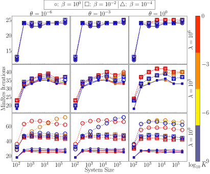
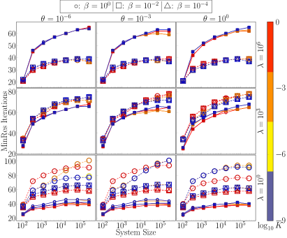
Figure 1: Performance of preconditioner $\mathcal{B}^{-1}_{1}$ in (3.9) (dashed lines) and block diagonal preconditioner $\mathcal{B}^{-1}_{2}$ in (3.27) (solid lines) for linear system due to (2.3) under varying $K$ (encoded by line color), $\beta$ (encoded by marks), $\theta$ (varies in subplots column-wise) and $\lambda$ (varies in subplots row-wise). Two realizations of the preconditioners are compared: (left) exact preconditioners, (right) approximation in terms of AMG.

Finally, we consider sensitivity to variations in $a_{0}$, $c_{0}$ holding the remaining parameters in (2.1) fixed at unit value. Our results are summarized in Table 3 where we report the iterations corresponding to mesh refinement levels $l$ with the mesh size $h=h_{0}/2^{l}$. We observe that the iterations are stable under varying $h$, $a_{0}$ and $c_{0}$.

	LU				AMG
	3	4	5	6	3	4	5	6
$(10^{1},10^{1})$	(25, 36)	(25, 36)	(25, 35)	(24, 35)	(35, 47)	(36, 48)	(37, 49)	(37, 49)
$(10^{1},10^{3})$	(24, 32)	(24, 32)	(24, 32)	(23, 32)	(35, 43)	(36, 45)	(36, 46)	(36, 46)
$(10^{1},10^{9})$	(12, 16)	(12, 16)	(12, 16)	(12, 16)	(17, 20)	(18, 22)	(18, 22)	(18, 22)
$(10^{3},10^{1})$	(24, 32)	(24, 32)	(24, 32)	(23, 32)	(35, 43)	(36, 45)	(36, 46)	(36, 46)
$(10^{3},10^{3})$	(23, 26)	(23, 26)	(23, 26)	(22, 26)	(33, 36)	(35, 37)	(35, 38)	(35, 38)
$(10^{3},10^{9})$	(12, 13)	(12, 13)	(12, 13)	(12, 13)	(17, 17)	(18, 19)	(18, 20)	(18, 20)
$(10^{9},10^{1})$	(12, 16)	(12, 16)	(12, 16)	(12, 16)	(17, 20)	(18, 22)	(18, 22)	(18, 22)
$(10^{9},10^{3})$	(12, 13)	(12, 13)	(12, 13)	(12, 13)	(17, 17)	(18, 19)	(18, 20)	(18, 20)
$(10^{9},10^{9})$	(10, 10)	(10, 10)	(10, 10)	(10, 11)	(16, 17)	(16, 18)	(18, 18)	(18, 18)

Table 3: Performance of preconditioners (3.9) and (3.27) for linear system due to (2.3) under varying $a_{0}$, $c_{0}$. The number of MinRes iterations is shown in the brackets where the first item is obtained using preconditioner (3.9). Realizations of the preconditioners in terms of LU and AMG are compared.

Remark 5.3 (Dense blocks due to $I_{0}$).

Due to the operator $I_{0}$ the matrix representation of both inner products $\mathcal{B}_{1}$ in (3.8) and $\mathcal{B}_{2}$ in (3.26) includes a dense block. In particular, let $\bm{x}\in\mathbb{R}^{n}$, such that $x_{i}=P_{m}\phi_{i}$ for all $\phi_{i}\in Q_{h}$ and $n=\text{dim }Q_{h}$ and let $\bm{y}=(\bm{x},\bm{0},\bm{0})$ be the representation of $(\phi,0,0)$ in $Q_{h}\times W_{h}\times W_{h}$. Then, the $Q$-block in the inner product (3.26) leading to block-diagonal preconditioner (3.27) and the $Q\times W\times W$-block in (3.8) yield operators

(5.2) $$\bm{A}_{2}-\bm{x}\bm{x}^{T},\quad\bm{A}_{1}-\bm{y}\bm{y}^{T}.$$

Here, the matrices $\bm{A}_{i}$ are symmetric and positive definite and the blocks thus have a structure of low-rank perturbed invertible operators. For example, with (3.26) the $Q$ block, which is the discretization of the inner product of $\lambda^{-1/2}L^{2}\cap L_{0}^{2}$, is represented as $\lambda^{-1}\bm{M}+(\bm{M}-\bm{x}\bm{x}^{T})$ with $\bm{M}$ the mass matrix of $Q_{h}$, see also [27]. In turn, $\bm{A}_{2}=(1+\lambda^{-1})\bm{M}$.

When computing the action of the preconditioners we take advantage of the structure (5.2) and invoke the Sherman–Morrison–Woodbury formula [20, Ch 2.1]

$$(\bm{A}-\bm{z}\bm{z}^{T})^{-1}=\bm{A}^{-1}+\frac{1}{1-\bm{z}^{T}(\bm{A}^{-1}\bm{z})}(\bm{A}^{-1}\bm{z})\bm{z}^{T}\bm{A}^{-1}.$$

Finally, the action of $\bm{A}^{-1}$ in the above formula is either computed with LU decomposition or approximated through AMG V-cycle. We note that, as $\bm{A}^{-1}\bm{z}$ can be precomputed once in the setup phase, the application of the preconditioner requires two evaluations of $\bm{A}^{-1}$.

Remark 5.4 (AMG in (3.9)).

The $3\times 3$ block of preconditioner (3.9) can present a challenge for parameter-robust approximations in terms of multilevel methods. In particular, assuming for simplicity mixed boundary conditions on the displacement, and letting $\gamma=\alpha\beta-b_{0}\lambda$ the inner product operator on $Q\times W\times W$ becomes

(5.3) $$\begin{bmatrix}I&0&0\\ 0&-t_{K}\text{div}(\nabla)+c_{0}I&0\\ 0&0&-t_{\theta}\text{div}(\nabla)+a_{0}I\end{bmatrix}+\frac{1}{\lambda}\begin{bmatrix}I&-\alpha I&-\beta I\\ -\alpha I&\alpha^{2}I&\gamma I\\ -\beta I&\gamma I&\beta^{2}I\\ \end{bmatrix}$$

and in certain parameter regimes the second term, which represents the coupling between $\xi$, $p$ and $T$, can become singular. As an example, setting $b_{0}=\beta=0$ the vector $(1,\alpha^{-1},0)^{T}$ can be seen to be in the kernel of the coupling operator. In this case, the strength of the singular perturbation is controlled by $1/\lambda$.

Algebraic multigrid methods for singularly perturbed elliptic operators have been developed e.g. in [28, 15]. Therein, a crucial ingredient for uniform performance with respect to the strength parameter is smoothers which capture the kernel. However, this condition is usually not met by pointwise smoothers, and block smoothers are required. Motivated by the analysis of [28, 15] we investigate the role of smoothers when realizing the Riesz map with respect to (5.3) by AMG. In order to simplify the realization of block smoothers let us consider a discretization of $Q_{h}$ and $W_{h}$ in terms of equal order elements, i.e. using $\mathbb{P}_{1}$ element for $W_{h}$ in (4.2). We shall then compare two AMG methods using point smoothers, namely BoomerAMG [17] and smoothed aggregation AMG (SAMG) [36], with SAMG utilizing block smoothers. The SAMG implementation was provided by PyAMG [4].

We evaluate the different approximations in terms of spectral condition numbers of (5.3) preconditioned by the AMG solvers. In Table 4 we observe that the performance of AMG with point smoothers is rather affected by parameter variations. On the other, block smoothers show little sensitivity. However, let us remark that parameter robust estimates in [28, 15] also require specialized prolongation operators which preserve the kernel. Here we have used standard prolongation instead.

	BoomerAMG				SAMG, point smoother				SAMG, block smoother
	3	4	5	6	3	4	5	6	3	4	5	6
($10^{-6}$, $10^{-9}$)	33.6	33.6	33	30.7	17.1	17	16.8	15.6	1	1	1	1
($10^{-6}$, $10^{-6}$)	33.6	33.5	32.5	29.2	17	17	16.5	14.8	1	1	1	1
($10^{-6}$, $10^{-3}$)	18.6	10.2	9.8	6.5	9.5	5.4	3.9	2.6	1	1	1	1.2
($10^{-6}$, 1)	6.6	7.3	7.5	7.5	1.5	1.4	1.5	1.8	1.2	1.4	1.4	1.6
($10^{-3}$, $10^{-9}$)	14.5	9.2	9.5	7.2	7.5	4.5	3.1	2	1	1	1.1	1.2
($10^{-3}$, $10^{-6}$)	14.5	9.2	9.5	7.2	7.5	4.5	3.1	2	1	1	1.1	1.2
($10^{-3}$, $10^{-3}$)	11.7	9.3	10.1	8.4	6.1	4.1	2.7	1.8	1	1	1.1	1.2
($10^{-3}$, 1.0)	6.6	7.2	7.4	8.2	1.4	1.4	1.5	1.8	1.2	1.3	1.4	1.7
(1, $10^{-9}$)	6	6.5	6.6	6.7	1.3	1.4	1.6	1.9	1.2	1.3	1.4	1.7
(1, $10^{-6}$)	6	6.5	6.6	6.7	1.3	1.4	1.6	1.9	1.2	1.3	1.4	1.7
(1, $10^{-3}$)	6	6.5	6.6	6.9	1.3	1.4	1.6	1.9	1.2	1.3	1.4	1.8
(1, 1)	5.2	5.5	5.6	5.6	1.8	4.1	15.5	67.2	1.2	1.4	1.5	1.8

Table 4: Spectral condition numbers of the Riesz map with respect to the inner product on $Q\times Q\times W$ induced by (3.8) when using different algebraic multigrid methods for preconditioning. A single V-cycle is always applied. Material parameters are as in Figure 1.

6 Conclusions and outlook

In this study, we investigated a four-field formulation of a linear thermo-poroelastic model, discretized using conforming finite elements. To address the challenges associated with parameter variations and discretization, we developed two robust preconditioners for the resulting linear system. Both preconditioners were demonstrated to be robust with respect to model parameters and discretization parameters, as confirmed through extensive numerical experiments. These results highlight the theoretical rigor and practical efficiency of the proposed preconditioners in solving linear thermo-poroelasticity problems in a parameter-robust and computationally effective manner.

Future research will focus on extending these methods to nonlinear thermo-poroelastic models. This includes developing efficient iterative algorithms and advanced preconditioners to handle the additional complexities introduced by nonlinearities. Furthermore, investigating the application of these techniques to large-scale and real-world problems and exploring decoupled and adaptive approaches will be crucial in enhancing the computational efficiency and accuracy of the methods in practical scenarios.

References

- [1] P. F. Antonietti, S. Bonetti, and M. Botti, Discontinuous Galerkin approximation of the fully coupled thermo-poroelastic problem, SIAM Journal on Scientific Computing, 45 (2023), pp. A621–A645.
- [2] O. Axelsson, R. Blaheta, and P. Byczanski, Stable discretization of poroelasticity problems and efficient preconditioners for arising saddle point type matrices, Computing and Visualization in Science, 15 (2012), pp. 191–207.
- [3] F. Ballarin, S. Lee, and S.-Y. Yi, Projection-based reduced order modeling of an iterative scheme for linear thermo-poroelasticity, Results in Applied Mathematics, 21 (2024), p. 100430.
- [4] N. Bell, L. N. Olson, J. Schroder, and B. Southworth, PyAMG: Algebraic multigrid solvers in Python, Journal of Open Source Software, 8 (2023), p. 5495.
- [5] M. A. Biot, General theory of three-dimensional consolidation, Journal of applied physics, 12 (1941), pp. 155–164.
- [6] M. A. Biot, Theory of elasticity and consolidation for a porous anisotropic solid, Journal of applied physics, 26 (1955), pp. 182–185.
- [7] S. Bonetti, M. Botti, and P. F. Antonietti, Robust discontinuous Galerkin-based scheme for the fully-coupled nonlinear thermo-hydro-mechanical problem, IMA Journal of Numerical Analysis, (2024), p. drae045.
- [8] W. M. Boon, M. Kuchta, K.-A. Mardal, and R. Ruiz-Baier, Robust preconditioners for perturbed saddle-point problems and conservative discretizations of Biot’s equations utilizing total pressure, SIAM Journal on Scientific Computing, 43 (2021), pp. B961–B983.
- [9] D. Braess, Stability of saddle point problems with penalty, RAIRO Modél. Math. Anal. Numér., 30 (1996), pp. 731–742, https://doi.org/10.1051/m2an/1996300607311, https://doi.org/10.1051/m2an/1996300607311.
- [10] S. C. Brenner, Korn’s inequalities for piecewise vector fields, Mathematics of Computation, (2004), pp. 1067–1087.
- [11] M. K. Brun, E. Ahmed, I. Berre, J. M. Nordbotten, and F. A. Radu, Monolithic and splitting solution schemes for fully coupled quasi-static thermo-poroelasticity with nonlinear convective transport, Computers & Mathematics with Applications, 80 (2020), pp. 1964–1984.
- [12] M. K. Brun, E. Ahmed, J. M. Nordbotten, and F. A. Radu, Well-posedness of the fully coupled quasi-static thermo-poroelastic equations with nonlinear convective transport, Journal of Mathematical Analysis and Applications, 471 (2019), pp. 239–266.
- [13] M. K. Brun, I. Berre, J. M. Nordbotten, and F. A. Radu, Upscaling of the coupling of hydromechanical and thermal processes in a quasi-static poroelastic medium, Transport in Porous Media, 124 (2018), pp. 137–158.
- [14] A. Budiša and X. Hu, Block preconditioners for mixed-dimensional discretization of flow in fractured porous media, Computational Geosciences, 25 (2021), pp. 671–686.
- [15] A. Budiša, X. Hu, M. Kuchta, K.-A. Mardal, and L. Zikatanov, Algebraic multigrid methods for metric-perturbed coupled problems, SIAM Journal on Scientific Computing, 46 (2024), pp. A1461–A1486.
- [16] Y. Chen and Z. Ge, Multiphysics finite element method for quasi-static thermo-poroelasticity, Journal of Scientific Computing, 92 (2022), p. 43.
- [17] R. D. Falgout and U. M. Yang, hypre: A library of high performance preconditioners, in Computational Sciences — ICCS 2002, P. M. A. Sloot, A. G. Hoekstra, C. J. K. Tan, and J. J. Dongarra, eds., Berlin, Heidelberg, 2002, Springer Berlin Heidelberg, pp. 632–641.
- [18] Z. Ge and D. Xu, Analysis of multiphysics finite element method for quasi-static thermo-poroelasticity with a nonlinear convective transport term, arXiv preprint arXiv:2310.05084, (2023).
- [19] V. Girault and P.-A. Raviart, Finite element methods for Navier-Stokes equations: theory and algorithms, vol. 5, Springer Science & Business Media, 2012.
- [20] G. H. Golub and C. F. Van Loan, Matrix computations, JHU press, 2013.
- [21] J. B. Haga, H. Osnes, and H. P. Langtangen, A parallel block preconditioner for large-scale poroelasticity with highly heterogeneous material parameters, Computational Geosciences, 16 (2012), pp. 723–734.
- [22] D. A. Ham, P. H. J. Kelly, L. Mitchell, C. J. Cotter, R. C. Kirby, et al., Firedrake User Manual, Imperial College London and University of Oxford and Baylor University and University of Washington, first edition ed., 5 2023, https://doi.org/10.25561/104839.
- [23] Q. Hong and J. Kraus, Parameter-robust stability of classical three-field formulation of Biot’s consolidation model, ETNA - Electronic Transactions on Numerical Analysis, 48 (2017).
- [24] Q. Hong, J. K. Kraus, M. Lymbery, and F. Philo, A new practical framework for the stability analysis of perturbed saddle-point problems and applications, Math. Comput., 92 (2023), pp. 607–634.
- [25] J. Kim, Unconditionally stable sequential schemes for all-way coupled thermoporomechanics: Undrained-adiabatic and extended fixed-stress splits, Computer Methods in Applied Mechanics and Engineering, 341 (2018), pp. 93–112.
- [26] A. E. Kolesov, P. N. Vabishchevich, and M. V. Vasilyeva, Splitting schemes for poroelasticity and thermoelasticity problems, Computers & Mathematics with Applications, 67 (2014), pp. 2185–2198.
- [27] J. J. Lee, K.-A. Mardal, and R. Winther, Parameter-robust discretization and preconditioning of Biot’s consolidation model, SIAM Journal on Scientific Computing, 39 (2017), pp. A1–A24.
- [28] Y.-J. Lee, J. Wu, J. Xu, and L. Zikatanov, Robust subspace correction methods for nearly singular systems, Mathematical Models and Methods in Applied Sciences, 17 (2007), pp. 1937–1963.
- [29] K.-A. Mardal and R. Winther, Preconditioning discretizations of systems of partial differential equations, Numerical Linear Algebra with Applications, 18 (2011), pp. 1–40.
- [30] R. Oyarzúa and R. Ruiz-Baier, Locking-free finite element methods for poroelasticity, SIAM Journal on Numerical Analysis, 54 (2016), pp. 2951–2973.
- [31] E. Piersanti, J. J. Lee, T. Thompson, K.-A. Mardal, and M. E. Rognes, Parameter robust preconditioning by congruence for multiple-network poroelasticity, SIAM Journal on Scientific Computing, 43 (2021), pp. B984–B1007.
- [32] A. P. Selvadurai and A. P. Suvorov, Thermo-poroelasticity and geomechanics, Cambridge University Press, 2016.
- [33] K. Terzaghi, Theoretical soil mechanics, 1943.
- [34] C. J. van Duijn, A. Mikelić, M. F. Wheeler, and T. Wick, Thermoporoelasticity via homogenization: modeling and formal two-scale expansions, International Journal of Engineering Science, 138 (2019), pp. 1–25.
- [35] C. J. van Duijn, A. Mikelić, and T. Wick, Mathematical theory and simulations of thermoporoelasticity, Computer Methods in Applied Mechanics and Engineering, 366 (2020), p. 113048.
- [36] P. Vanek, J. Mandel, and M. Brezina, Algebraic multigrid by smoothed aggregation for second and fourth order elliptic problems, Computing, 56 (1996), pp. 179–196.
- [37] J. Zhang and H. Rui, Galerkin method for the fully coupled quasi-static thermo-poroelastic problem, Computers & Mathematics with Applications, 118 (2022), pp. 95–109.
- [38] J. Zhang and H. Rui, A coupling of Galerkin and mixed finite element methods for the quasi-static thermo-poroelasticity with nonlinear convective transport, Journal of Computational and Applied Mathematics, 441 (2024), p. 115672.