AutoG: Towards automatic graph construction from tabular data

Abstract

Recent years have witnessed significant advancements in graph machine learning (GML), with its applications spanning numerous domains. However, the focus of GML has predominantly been on developing powerful models, often overlooking a crucial initial step: constructing suitable graphs from common data formats, such as tabular data. This construction process is fundamental to applying graph-based models, yet it remains largely understudied and lacks formalization. Our research aims to address this gap by formalizing the graph construction problem and proposing an effective solution. We identify two critical challenges to achieve this goal: 1. The absence of dedicated datasets to formalize and evaluate the effectiveness of graph construction methods, and 2. Existing automatic construction methods can only be applied to some specific cases, while tedious human engineering is required to generate high-quality graphs. To tackle these challenges, we present a two-fold contribution. First, we introduce a set of datasets to formalize and evaluate graph construction methods. Second, we propose an LLM-based solution, AutoG, automatically generating high-quality graph schemas without human intervention. The experimental results demonstrate that the quality of constructed graphs is critical to downstream task performance, and AutoG can generate high-quality graphs that rival those produced by human experts.

1 Introduction

Graph machine learning (GML) has attracted massive attention due to its wide application in diverse fields such as life science (Wong et al., 2023), E-commerce (Ying et al., 2018), and social networks (Wang & Kleinberg, 2023; Suárez-Varela et al., 2022). GML typically involves applying models like graph neural networks (GNNs) (Kipf & Welling, 2017) to leverage the underlying graph structure of a given task, e.g., using the friendship networks for user recommendations (Tang et al., 2013) and identifying new drug interactions  (Zitnik et al., 2018).

Despite the widespread interest and rapid development in GML (Kipf & Welling, 2017; Mao et al., 2024; Müller et al., 2024), constructing graphs from common data formats such as industrial tabular data (Ghosh et al., 2018) remains an under-explored topic. This primarily stems from a widely adopted assumption that appropriate graph datasets exist for downstream tasks akin to established benchmarks (Hu et al., 2020; Khatua et al., 2023). However, readily available graph datasets are absent in many real-world enterprise scenarios. First, given an input data in common storage formats such as tables, there can be many plausible graph schemas and structures that can be defined over them. The choice of graph schema impacts downstream performance of GML. Rossi et al. (2024) shows that considering the directional aspect of edges within a graph can lead to substantial variance in the downstream GML performance. Second, converting the source data into graph format requires expert data engineering and processing. Even though, GNN based approaches shows strong performance on Kaggle leaderboard (Wang et al., 2024b), it involves laborious pre-processing and specialized skills to transform the original tabular data into ready-to-be-consumed graphs for GML.

The objective of this work is to formalize the challenges in graph construction by establishing real-world datasets followed by automatic graph construction from input tabular data. Existing tabular graph datasets such as Wang et al. (2024b) and Fey et al. (2024) assume the availability of well-formatted graphs with explicit relationships such as complete foreign-key and primary-key pairs. In these cases, graphs can be easily constructed using heuristics like Row2Node (Cvitkovic, 2020) by converting each table into a node type. However, implicit relationships like columns with similar semantics (Dong et al., 2023) or columns with categorical types also widely exist in real-world scenarios, which cannot be addressed by heuristic methods (see Figure 1). Datasets designed for evaluating graph construction should reflect the importance of modeling implicit relationships. Additionally, different tasks can be defined based on the same dataset (Fey et al., 2024). Further, different ways to construct graphs affect different tasks’ performance is an understudied problem. Therefore, ideal datasets for graph construction should also include different downstream tasks to reflect this problem. From the solution perspective, graph construction involves finding the best candidate among all possible graph structures. However, considering the vast search space, finding the graph structure through an exhaustive search is infeasible. Therefore, an effective automatic graph construction method should be able to efficiently identify high-quality candidates from many possible graph structures/schemas.

To address the above challenges, we propose a set of evaluation datasets and a large language model (LLM)-based graph construction solution. We first extract raw tabular datasets from Kaggle, Codalab, and other data sources to design datasets reflecting real-world graph construction challenges. They differ from prior work (Fey et al., 2024; Wang et al., 2024b) in that these datasets haven’t been processed by experts, and existing graph construction methods get inferior performance (see Table 3). To solve the graph construction problem, we propose an LLM-based automatic graph construction solution AutoG inspired by LLM’s reasoning capability to serve as a planning module for agentic tasks (Zhou et al., 2024) and tabular data processing (Hollmann et al., 2023). However, we observe that LLMs tend to generate invalid graphs or graphs with fewer relationships (as shown in Section 5.3.1). We address this problem by guiding LLMs to conduct close-ended function calling (Schick et al., 2024). Specifically, we decompose the generation of graph structures into four basic transformations applied to tabular data: (1) establishing key relations between two columns, (2) expanding a specific column, (3) generating new tables based on columns, and (4) manipulating primary keys. Coupled with chain-of-thought prompt demonstrations for each action, AutoG generates a series of actions to get the augmented schema and thus construct the graph. To further enhance the generation quality, it will adopt the early-stage validation performance of trained GML models as an oracle to select results efficiently.

Our major contributions can be summarized as follows:

1. Formalizing graph construction problems with a set of datasets: We create a set of datasets covering diverse graph construction challenges, consisting of eight datasets from academic, E-commerce, medical, and other domains.

2. LLM-based automatic graph construction method: AutoG: To solve the graph construction problem without manual data engineering, we propose an LLM-based baseline to automatically generate graph candidates and then select the best candidates efficiently.

3. Comprehensive evaluation: We compare AutoG with different baseline methods on the proposed datasets. AutoG shows promising performance that is close to the level of a data engineering expert. Among $12$ test tasks, it achieves $98.5\%$ of the performance of human expert-designed prompts on $9$ downstream tasks.

2 Preliminaries

2.1 tabular data and schemas

The input tabular data is represented using the RDB language (Codd, 2007; Chen, 1976) as a schema file. Subsequently, we introduce table schemas and how they may be used to describe a graph. We start by introducing the fundamental elements of RDB languages.

Definition. Tabular data $\mathcal{D}$ contains an array of $K$ tables $\mathcal{D}:=\left\{T_{i}\right\}_{i=1}^{K}$. Each table $T_{i}$ can be viewed as a set $T_{i}=\left(C_{i},R_{i},M_{i}\right)$, where

• $C_{i}=(C_{i,1},\dots,C_{i,l_{i}})$ is an array of strings representing the column names, with $l_{i}$ denoting the number of columns in $T_{i}$.

• $R_{i}$ is a matrix where each row $R_{i,j}=(R_{i,j,1},\dots,R_{i,j,l_{i}})$ contains the values for the $j$-th row of table $T_{i}$.

• $M_{i}=(M_{i,1},\dots,M_{i,l_{i}})$ is an array specifying the data type of each column.

In this paper, we consider the following data types {category, numeric, text, primary_key(PK), foreign_key (FK), set, timestamp}. As an example, if $M_{i,1}=\texttt{text}$, then all values in the same column $R_{i,1,1},\cdots,R_{i,m_{i},1}$ are of text type ($m_{i}$ refers to the number of rows for table $T_{i})$. Detailed descriptions of each data type can be found in Appendix A.1.

The definitions above focus on the properties of individual tables, For multiple tables with $K>1$, they can be related with set of $n$ PK-FK pairs $\left\{x_{\texttt{PK}}^{m},y_{\texttt{PK}}^{m},x_{\texttt{FK}}^{m},y_{\texttt{FK}}^{m}\right\}$ where $m=1,\ldots,M$. $x$ and $y$ represent the indices of tables in $\mathcal{D}$ and the indices of columns. In real-world scenarios, it’s often the case that only a subset of all PK-FK are explicit (Wang et al., 2024b). The other implicit connections must be identified manually to support downstream tasks well.

Table schema and graph schema description. Based on this language, we define table schema by storing all the meta information in a structured format like YAML (Ben-Kiki et al., 2009). An example is shown in Appendix A.2. Table schema defines the metainformation of tables in a structured manner following the RDB language. Graph schema is a special type of table schema. Compared to general table schema, graph schema presents tables with proper column designs and PK-FK relations. These characteristics make it trivial to convert a graph schema (as discussed in Section 2.2) into an ideal graph structure for downstream tasks.

2.2 Bridging tabular data and graphs

Based on the definition of tabular data, the goal of graph construction is to convert relational tabular data $\mathcal{D}$ into a graph $\mathcal{G}$. Following Fey et al. (2024); Wang et al. (2024b), we consider $\mathcal{G}$ as a heterogeneous graph (Wang et al., 2022) $\mathcal{G}=\{\mathcal{V},\mathcal{E}\}$ characterized by sets of nodes $\mathcal{V}$ and edges $\mathcal{E}$. The nodes and edges are organized such that $\mathcal{V}=\bigcup_{v\in V}\mathcal{V}^{v}\text{ and }\mathcal{E}=\bigcup_{e\in E}\mathcal{E}^{e}$ where $\mathcal{V}^{v}$ represents the set of nodes of type $v$, and $\mathcal{E}^{e}$ represents the set of edges of type $e$. The main challenge of graph construction lies in extracting appropriate node types and edge types from the schema of tabular data. This process could be straightforward if we treat each table as a node type and each PK-FK relationship as an edge type. However, this method may generate suboptimal graphs for general table schemas. For instance, when two entities are placed in a single table, one entity might be treated as a feature of the other, resulting in a graph that fails to effectively reflect structural relationships, thereby impacting the performance of downstream tasks (Wang et al., 2024b).

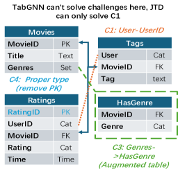
(a) Movielens

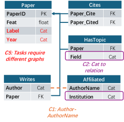
(b) MAG

Figure 1: Demonstrations of challenges in two selected datasets. Existing heuristic-based methods cannot well tackle C2-C5 in that they require task-specific decisions.

3 Designing datasets for evaluating graph construction

To make the graph construction problem concrete and provide a set of datasets for comparing different methods, we first identify key problems that need to be addressed during the graph construction process, which can be viewed as the design space. Based on these problems, we have carefully selected $8$ multi-tabular datasets from diverse domains to construct datasets for graph construction.

3.1 Design space of the datasets

We propose four core challenges to be addressed when converting tabular data into graphs. Examples of these challenges are demonstrated in Figure 1.

1. C1: Identifying edges from non PK-FK relationships: Traditional methods like Row2Node (Wang et al., 2024b) only turn PK-FK relationships into edges, while these relationships are usually not complete, which necessitates either automatic join discovery (Dong et al., 2023) or human intervention.

2. C2: Augmenting multiple node or edge types from one table: Multiple node types and edge types may be improperly put in one table. For example, the “Field” column in Figure 1 can induce useful relations, and thus, an augmented table should be added.

3. C3: Transforming tables into proper node or edge types: How to convert tables into appropriate types affects downstream task performance and the validity of generated graphs. For instance, the “Ratings” table in Figure 1 should be better modeled as an edge type since it’s about predicting the property between user and movie type.

4. C4: Generating proper graphs for different downstream tasks: Considering that multiple tasks can be defined based on the same tabular data (Fey et al., 2024), one single graph design may not fit all tasks. This claim has not been well studied and will be verified in the experiment.

Design philosophy of these challenges. These four challenges are inspired by existing works (Wang et al., 2024b; Dong et al., 2023; Gan et al., 2024) but go beyond their scopes. Specifically, C1 is a common problem in data lakes and RDB (Dong et al., 2023; Hulsebos et al., 2019) for automatic data engineering. When constructing the graph is the final objective, joinable column detection becomes even more important since it’s crucial to find relations. C2 is derived by comparing the original schema from Kaggle to the graph schema used in Wang et al. (2024b). Human experts have introduced multiple augmented tables, which are crucial to the performance of GML models. The mechanism behind these augmented tables hasn’t been well studied, and we first introduce them in our datasets. C3 is derived from real-world datasets such as (Harper & Konstan, 2015), and we find that simple heuristics may work poorly when the proper type of table cannot be induced from the schema. C4 is naturally derived from the multiple tasks defined on tabular data. We are the first to study the influence of graphs on different downstream task performance.

Relationship to traditional database profiling (Abedjan et al., 2015). Database profiling, including normalization, is a related concept to our work. The goal of graph construction from relational data to graph is to find what kind of relational information is beneficial to the downstream task. For example, the objective of challenge 2 is to consider whether the relationship induced by this categorical value is beneficial. This decision needs to consider the semantic relationship between this column and the corresponding downstream tasks, which cannot be solved by normalization. As a comparison, profiling aims to minimize data redundancy and improve data integrity. Despite the overlap, data profiling method cannot fully solve the graph construction task.

3.2 Datasets

Based on the design space of graph construction from relational tabular data, we gather $8$ datasets from various domains to evaluate graph construction methods. We collect these datasets from 1. the source of existing tabular graph datasets, such as Diginetica (Wang et al., 2024b); 2. augmented from existing tabular graph datasets, such as Stackexchange (Wang et al., 2024b); 3. traditional tabular datasets adapter for graph construction, including IEEE-CIS (Howard et al., 2019) and Movielens (Harper & Konstan, 2015). The information of these $8$ datasets is listed in Table 1. Two concrete examples are shown in Figure 1. Details on dataset sources and pre-processing are shown in Appendix B.

Table 1: Our proposed datasets. The tasks are categorized into predictions of relation attribute, entity attribute, and FK by following (Wang et al., 2024b).

Name of the dataset	#Tasks	#Tables	Inductive	C1	C2	C3	C4	Task type	Source of datasets
Movielens	1	3	✓	✓	✓	✓	✗	Relation Attribute	Designed from Harper & Konstan (2015)
MAG	3	5	✗	✓	✓	✓	✓	Entity Attribute, FK Prediction	Augmented from Wang et al. (2024b)
AVS	2	3	✓	✓	✓	✓	✓	Entity Attribute	Augmented from Wang et al. (2024b)
IEEE-CIS	1	2	✗	✗	✓	✓	✗	Entity Attribute	Designed from Howard et al. (2019)
Outbrain	1	8	✓	✓	✓	✓	✗	Relation Attribute	Augmented from Wang et al. (2024b)
Dignetica	2	8	✓	✓	✓	✓	✓	Relation Attribute, FK Prediction	Augmented from Wang et al. (2024b)
RetailRocket	1	5	✓	✓	✓	✓	✗	Relation Attribute	Augmented from Wang et al. (2024b)
Stackexchange	3	7	✓	✓	✓	✓	✓	Entity Attribute	Augmented from Wang et al. (2024b)

Evaluation. To evaluate the quality of generated graphs, we adopt a quantitative evaluation approach by assessing downstream task performance, i.e., use fixed GML models (RGCN, RGAT, HGT, R-PNA) to compare the impact of different graph construction methods. Better downstream task performance indicates higher graph quality. We consider both the performance of individual models and the average performance of different models.

4 Method

This section introduces an automatic graph construction solution to tackle the five challenges in Section 3.1. As discussed in Section 2.2, we consider graph construction as a transformation from the original table schema with implicit relations to the final graph schema with explicit relations. We adopt an LLM as the decision maker to generate transformations automatically.

4.1 AutoG: An LLM-based graph construction framework

Inspired by the classic generator-discriminator structure (Goodfellow et al., 2014), we first design a generator to produce reasonable candidates, and then evaluate the generated results through a discriminator. In previous work (Fey et al., 2024; Wang et al., 2024b), human data scientists often play the generator, which generates outputs based on their expert knowledge. Like humans, LLMs also demonstrate the capabilities to generate molecular structures or code-formatted augmentations based on prior knowledge (Wang et al., 2024a; Hollmann et al., 2023). Consequently, we adopt an LLM as a generator and provide it with input tabular data to generate transformations. As demonstrated in Figure 2, we propose a framework AutoG composed of the following modules.

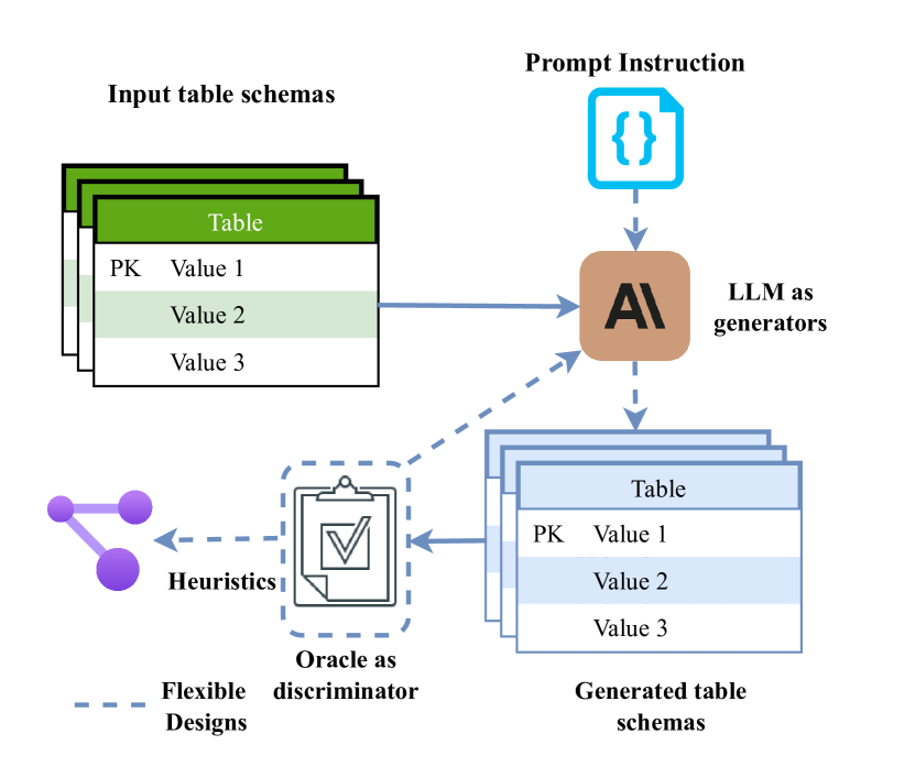
Figure 2: An illustration of our proposed AutoG framework.

Input module. The input of AutoG consists of two parts. The first part is the input table schema, which represents the metadata related to the data. The second part is the prompt instruction. Following Wang et al. (2024b), we use the table schema format introduced in Section 2.1 to represent the input data. An example can be found in Appendix A.2. Input schema files can be easily generated from tabular storage (e.g., Pandas DataFrames), with column data types either user-defined or inferred from sampled column values using LLMs (see Appendix D.4). For prompt instruction, we include a general description of the graph construction task, a one-sentence description for the corresponding downstream task, and data supplementary information, including dataset statistics and sample column values.

LLM as generators. Based on input modules, we further leverage LLMs to generate a transformed schema. A straightforward approach is to let the LLM directly generate structured outputs such as YAML (Ben-Kiki et al., 2009)-formatted code. However, we find that open-ended generation usually produces invalid graph structures. To address this, inspired by the idea of function calling (Schick et al., 2024), we design basic augmentation actions based on $5$ challenges of graph construction and then guide the output through chain-of-augmentation prompts, which is elaborated in Section 4.2.

Heuristic-based graph constructors. We then employ heuristic algorithms to convert tables into graphs once a candidate table schema is generated. For instance, if we opt for the Row2Node/Edge heuristic algorithm, we transform tables with at least two columns as FK and no PK, along with the remaining PK-FK relationships, into edges of a heterogeneous graph, while converting other tables into nodes.

Oracle as discriminators. After generating the graph, we design an oracle as a discriminator to generate feedback. LLMs generate candidate results based on the semantic information and statistics of tables. This information can serve as valuable priors but cannot evaluate the validity and compatibility of the generated graphs with specific downstream tasks. As a result, we adopt either the results of graph construction (whether successful or not) or execute a GML model training module to get the (estimated) performance of the generated graph. Such feedback will further be appended to the prompt instruction as history information. We detail the oracle design in Section 4.3.

4.2 Guided generation with Chain-of-augmentation

The most straightforward way to let LLMs generate schema is directly generating the YAML-formatted structured outputs. However, such open-ended generation suffers from the following pitfalls: 1. LLMs generate schema and augmentation code with grammar errors, which makes the pipeline fail to proceed automatically. 2. LLMs tend to miss those node types and relations that require multi-step augmentation. Taking the Diginetica dataset as an example, relations may be found by first transforming set-attributed columns into proper augmented columns and then identifying the non PK-FK relations from the augmented columns. Simply generating the schema in a single-step manner fails to extract such relations.

To alleviate these problems, we propose guided generation with a chain of augmentation. First, based on four challenges proposed in Section 3.1, we identify the following basic actions for augmentation.

1. CONNECT_TWO_COLUMNS: Building a PK-FK relationship between two columns, and it will first make sure they satisfy the PK constraints. This action is designed to tackle challenge 1. Compared to joinable table discovery (JTD) (Dong et al., 2023; Hulsebos et al., 2019), this action is simpler because it directly generates the potential column pairs based on LLM decisions. JTD can also be used as a replacement in scenarios requiring higher accuracy with the cost of much more running time.

2. GENERATE_NEW_TABLE: Inducing a new table from the original table via moving columns without changing any values. This can be viewed as identifying multiple node or relation types from the original table. This action is designed to tackle challenge 2.

3. REMOVE(ADD)_PRIMARY_KEY: Combined with proper heuristic methods, this action can change the type of table (as a node or an edge type) in the generated graph. This action is designed to tackle challenge 3.

We then provide two types of supplementary information in the prompt to help LLMs decide on actions. Statistics of columns: A textual description of the task and statistics of each column are appended to the prompt instruction, guiding the LLM’s decision-making. LLM will determine the usefulness of actions like GENERATE_NEW_TABLE based on whether the augmented table semantically contributes to the task. For instance, if the task is to identify citations between papers, the “co-author” relationship is highly relevant, and the LLM will favor generating a table representing such a relation. Conversely, the “co-year” relationship is less informative, making the LLM less likely to generate it. Additionally, if a categorical column has only two distinct values, the induced table will become a super node in the graph, which is not ideal for model training, thus the LLM will tend not to generate such a table. Chain of thought demonstrations: For each of these actions, we provide a demonstration to showcase its usage. Specifically, we find that chain-of-thought (CoT) prompts (Wei et al., 2022) are critical to action generation. As a motivating example, LLMs tend to merely find those columns with identical names to build non-PK-FK relationships without CoT. Only after introducing CoT demonstrations can LLMs utilize the statistics of columns to find more general non-PK-FK relationships with different column names. The complete prompt design can be found in Appendix D.1. To determine the termination step, we add a null action to the action space and set a hard threshold $T$ to limit the maximum number of actions, typically set to $10$ for our proposed datasets.

4.3 Designing oracle to generate feedback

After generating the schema candidates, we need an oracle to evaluate their effectiveness and thus choose the best schema. Despite LLM’s capability to generate schemas based on prior knowledge, they cannot quantitatively predict how different schemas affect downstream task performance. As a result, we still need a graph-centric model to generate the feedback. We introduce qualitative and quantitative oracles, where the former checks the validity of schemas by running graph construction heuristics, and the latter adopts the GML model to determine the quality of graph schema. We detail the quantitative oracle exploration below.

Table 2: Evaluating different oracles by quality and efficiency. For sampling, we set the ratio to 30%. For early-stage validation performance, we set to $10\%$ of total epochs (should be set according to different datasets). NetInfoF can’t be applied to large-scale link prediction here since compatibility matrix computation is not scalable. The pre-processing time of the full graph is set as the basic unit; all other time is rounded to an integer.

	Discrepancy	Training (node)	Training (link)	Process
Full	0	29x	300x	1x
Sampled	0.75	16x	95x	1x
Actively sampled	0.75	16x	95x	3x
Early metric	0.09	10x	52x	1x
NetInfoF	Not applicable

The main challenge of designing a quantitative oracle is to efficiently obtain the approximate performance of models. After using heuristics to construct graphs based on the generated schemas, AutoG will automatically execute the GML model fitting process, and the validation performance will be adopted as the final metric. We further explore the potential to speed up this process: (1) Condensating the graph (Hashemi et al., 2024), improving the evaluation efficiency by training and testing on a smaller graph; (2) Adopting an early-stage training metric, such as the validation set performance. (3) Simplified or Training-free model: Adopting a simplified model such as linear GNN (Yu et al., 2020; Lee et al., 2024) designed for heterogeneous graphs. However, we find that existing linear GNNs for heterogeneous graphs can only achieve embeddings for target nodes, which does not apply to general link-level prediction (more discussion in Appendix D.3). We then compare these methods in terms of their effectiveness and efficiency. Specifically, we randomly sample three groups of schemas (in total $36$, with distinguishable performance) from the proposed datasets. Then, we let different oracles generate orders for each group and measure the normalized Kendall’s tau distance (Kumar & Vassilvitskii, 2010) to ones generated by regular GML models. From the experimental results in Table 2, we find that only the early-stage validation performance can estimate the downstream task performance well, as adopted in AutoG.

4.4 Candidate and result generation

After describing the LLM’s action space and oracle, the last part of AutoG is the candidate generation strategy. Instead of using complex tree-based search strategies like MCTS (Zhang et al., 2024a), we use a simpler strategy that generates one action at a time to create a new candidate. We find that tree-based search cannot improve the generated candidate quality and many candidates are duplicated. AutoG will backtrace to the last valid states when an invalid action is generated and terminate after consecutive errors. To produce diverse schemas, we run the algorithm multiple times and choose the candidates with the best oracle score as the final selection.

5 Experimental Results

In this section, we systematically evaluate the AutoG framework on the proposed benchmarks from the following perspectives:

• Quantitative Evaluation: Comparing variants of AutoG to other heuristic-based graph construction algorithms and expert-designed graph schemas.

• In-depth Analysis: Conducting ablation studies on different components of AutoG to understand the mechanism and limitations of AutoG.

5.1 Experimental settings

To investigate the impact of different graph construction methods, we fix the GML model to check the downstream task performance according to different graph schemas. Specifically, we select two commonly used baselines on heterogeneous graphs, RGCN (Schlichtkrull et al., 2018) and RGAT (Veličković et al., 2018). We present the RGCN results and show RGAT ones in Appendix E.1. On the constructed graph, we choose the optimal hyperparameters based on the model’s performance on the validation set, with the selection range detailed in appendix D.2. We select Claude’s Sonnet-3.5 as the backbone of LLMs and investigate the impact of different LLMs in Section 5.3. We consider the following baseline methods:

• XGBoost (Chen & Guestrin, 2016) and DeepFM (Guo et al., 2017): Directly applying XGBoost and DeepFM, two widely adopted baselines for tabular data to the merged tables.

• TabGNN (Guo et al., 2021): Creating an edge type based on every categorical value and constructing a multiplex graph based on each edge type.

• Row2Node and Row2Node/Edge (Wang et al., 2024b): Converting tables to graphs with heuristics. Row2Node treats each table as a node type and each PK-FK relationship as an edge type. Row2Node/Edge introduces more flexibility by treating tables with two FK columns as an edge between the FK-induced pair.

• JTD with Row2Node/Edge (Dong et al., 2023; Gan et al., 2024): Joinable table discovery (JTD) targets finding joinable columns across tables. It can be combined with heuristics to generate graphs with more complex relations.

• Graph schema designed by human experts. We detail the expert schema design in Appendix E.3.

5.2 Quantitative evaluation

Table 3 shows the performance of different graph construction methods. Our evaluation follows the following steps: (1) generate the heterogeneous graphs with the corresponding graph construction methods; (2) then, train a GML model towards downstream tasks with the constructed graph. Models’ performance is used to determine the quality of graphs. We consider both the individual model performance and average model set’s performance. We show the performance of RGCN, ranking of RGCN, and ranking of average performance in Table 3. The metrics for each task are shown in the second column, and the ranking is calculated based on the average ranking of each task.

Table 3: Evaluation of different graph construction methods on proposed datasets. The best is in bold, second best is underlined, and third best is double-underlined.

Dataset	Task	XGBOOST	DeepFM	TabGNN	Original schema		JTD schema		AutoG	Expert
		N/A	N/A	TabGNN	R2N	R2NE	R2N	R2NE	AutoG	Expert
Datasets with a single downstream task
IEEE-CIS	Fraud (AUC)	90.14	90.28	75.38	89.17	89.17	89.17	89.17	90.36	89.20
RetailRocket	CVR(AUC)	50.35	49.33	82.84	50.45	49.90	50.82	48.99	82.53	84.70
Movielens	Ratings(AUC)	53.62	50.93	55.34	57.34	56.96	54.55	64.71	66.54	66.54
Outbrain	CTR(AUC)	50.05	51.09	62.12	49.33	52.06	49.35	52.23	61.32	62.71
AVS	Repeat (AUC)	52.71	52.88	54.48	47.75	48.84	53.27	53.27	54.03	55.08
Datasets with multiple downstream tasks
MAG	Venue (Acc)	21.95	28.19	42.84	27.24	46.26	21.26	46.97	49.88	49.66
	Citation (MRR)	3.29	45.06	70.65	65.29	65.29	72.53	81.50	80.84	80.86
	Year (Acc)	28.09	28.42	52.77	54.09	30.90	53.07	53.07	54.09	35.35
Dignetica	CTR (AUC)	53.50	50.57	50.00	68.44	65.92	50.05	50.00	72.26	75.07
	Purchase (MRR)	3.16	5.02	5.01	5.64	7.70	11.37	15.47	34.92	36.91
Stackexchange	Churn(AUC)	58.20	59.84	78.27	74.23	75.62	85.58	84.85	85.43	85.58
	Upvote(AUC)	86.69	87.64	85.28	88.49	88.65	88.61	67.98	88.57	88.61
Ranking (RGCN)		5.8	5.2	4.3	4.5		4.1		2.0	1.8
Ranking (Average)		5.8	5.5	4.5	4.5		3.4		2.3	1.9

From the experimental results, we make the following observations

• AutoG generates high-quality graphs: The AutoG method we propose can surpass other automatic graph construction methods and reach close to the level of human experts.

• AutoG’s superiority against heuristic-based methods: Heuristic-based automatic discovery methods can only be applied to some special cases. We particularly note that AutoG has a unique advantage in addressing challenge 2. Unlike challenge 1, challenge 2 is originally solved entirely based on expert experience. Take IEEE-CIS as an example, which has many categorical columns. If all categorical columns are converted into relations, it will lead to poor performance (TabGNN). In contrast, AutoG, based on LLMs, can analyze the semantic relationships between columns, for instance, grouping all card-related meta information into one table (see Appendix E.3), thus achieving good results.

• The same graph may not be effective for different downstream tasks. On the MAG dataset, we observe that the expert-designed graph is not optimal for the year prediction task and is much worse than the original schema. This demonstrates the importance of adaptively generating graphs based on the task and illustrates the importance of automatic graph construction. Taking a deeper look at the generated graph statistics, we find that when predicting the venue of “Paper”, the adjusted homophily (Lim et al., 2021) of labels based on metapath “Paper-Author-Paper” is $0.156$. While for year prediction, the adjusted homophily is only $0.02$. This can be viewed as an extension of the heterophily problem (Lim et al., 2021) towards the RDB data, and an effective graph construction algorithm should address this problem by eliminating harmful relations. AutoG still relies on a graph oracle to deal with this problem. As shown in Appendix E.1, the observation based on RGAT is consistent.

5.3 In-depth analysis

To better understand the effectiveness of AutoG, we further study the effect of its components. We conduct three experiments: (1) Comparing AutoG variants with open-ended generation and oracle-free designs. (2) Studying the effect of different LLM backbones on the final results. (3) Studying the necessity of each prompt component. We also study AutoG’s performance on synthetic data with anonymous columns.

Table 4: Ablation studies for closed-ended generation and oracles

Dataset	Task	Valid			Performance
		AutoG-S	AutoG-A	AutoG	AutoG-A	AutoG
MAG	Venue	✗	✓	✓	49.88	49.88
	Year	✗	✓	✓	35.40	54.09
IEEE-CIS	Fraud	✗	✓	✓	90.15	90.36
RetailRockets	CVR	✗	✓	✓	82.53	82.53

Table 5: Effect of LLMs on generation validity and performance. *CoT prompts doesn’t work for Mistral.

LLM	MAG (venue)			Movielens (ratings)
	#actions	Valid	Best	#actions	Valid	Best
Sonnet3.5	4	100%	✓	7	57%	✓
Sonnet3	8	37.5%	✓	4	75%	✗
Mistral(*)	7	57%	✓	2	22%	✗

5.3.1 AutoG Variants Studies

We consider two variants of AutoG: AutoG-S and AutoG-A, where AutoG-S presents no pre-defined actions, and AutoG-A removes oracles from AutoG. As shown in Table 5, we draw the following conclusions: 1. Close-ended generation is necessary for valid schema generation. 2. Oracle is often unnecessary, meaning LLMs can generate good candidates merely based on prior knowledge. However, AutoG-A also performs poorly in some specific tasks with potentially noisy relations, as discussed in Section 5.2. A viable next step for our method would be determining whether an oracle is needed before running AutoG, which could improve overall efficiency.

5.3.2 Influence of LLMs

We then evaluate the influence of different LLMs. We mainly compare three typical models: Claude Sonnet 3.5, Mistral Large, and Claude Sonnet 3. As shown in Table 5, we find that 1. more powerful LLMs generate better schemas with fewer invalid actions, which may be related to the instruction following capability. 2. We observe that CoT demonstrations work poorly for Mistral Large, which may be due to different LLMs’ distinct pre-training strategies. Generally, we find that for LLM models with capabilities surpassing Sonnet3, AutoG can generate promising results and surpass heuristic-based counterparts.

5.3.3 Working mechanism of AutoG

Table 6: Ablation studies of different AutoG prompt components. “Orig” stands for the original schema with original names. “Anon” stands for the anonymous column names. “3/3” means $3$ of the $3$ expected actions have all been generated.

	Challenge 1		Challenge 2		Challenge 3
	Orig	Anon	Orig	Anon	Orig	Anon
Default	3/3	1/3	2/3	1/3	2/2	0/2
No COT	1/3	0/3	1/3	0/3	0/2	0/2
No stats	1/3	0/3	1/3	0/3	0/2	1/2
No demon	0/3	0/3	0/3	0/3	0/2	0/2

Despite the promising performance of AutoG, LLM as generators is composed of complicated prompt designs, which makes it challenging to understand the role of each component and how they may be applied to more general types of tabular data (for example, ones with anonymous columns). We thus further study the influence of different prompt components. In our prompt design, we have considered the following components: 1. the semantic information of the column (column name); 2. the statistical meta-information of the column; 3. the examples given in the prompt; 4. the chain of thought demonstrations for each action. Specifically, we built a synthetic dataset based on MAG to include the challenges $1-4$ proposed in Section 3.1 and ensure the test data is not included in the pre-training set of LLMs. Compared to quantitative evaluation, here we directly study whether LLMs can generate the required actions for better graphs. As shown in Table 6, we observe the following conclusions: 1. Demonstration is necessary for AutoG to generate valid actions. 2. Both COT and statistics are critical to the graph schema generation. Specifically, we find that LLMs will only find trivial augmentations (for example, non-PK-FK relations with identical column names), which means COT is the key for LLMs to conduct deep reasoning and to well utilize the statistics. 3. Semantic information of the column names is vital for the performance of AutoG, which is a limitation of AutoG. Column name expansion (Zhang et al., 2023a) may be adopted to enhance the effectiveness of AutoG on anonymous data.

6 Related Works

Recently, GML has been widely adopted to capture the structural relationship across tabular data (Li et al., 2024). One of the key challenges lies in identifying graph structures from tabular data that can benefit the downstream tasks. Early endeavors in database management mine relationships across databases using rule-based methods Yao & Hamilton (2008); Liu et al. (2012); Abedjan et al. (2015); Koutras et al. (2021). One limitation of these methods lies in their scalability towards large-scale tables. The rise of machine learning has led to two ML-based approaches: heuristic-based and learning-based methods. Heuristic-based methods transform tabular data into graphs based on certain rules. For instance, Guo et al. (2021) generates edge relationships based on columns with categorical values in the table, resulting in a multiplex graph through multiple columns. Wu et al. (2021) and You et al. (2020) create a bipartite graph based on each row representing a sample and each column representing a feature, where You et al. (2020) further supports numerical values by storing them as edge attributes. Du et al. (2022) generates a hypergraph by treating each row as a hyperedge. A major challenge for these heuristic methods is the inability to handle multi-table scenarios effectively. Row2Node (Fey et al., 2024) and Row2Node/Edge (Wang et al., 2024b) are proposed for multiple tables with explicit key relationships. Bai et al. (2021) designs and end-to-end model for RDB prediction tasks. These methods are still limited to tables satisfying RDB specifications. Learning-based methods aim to learn edge relationships automatically based on the correlation between features. Chen et al. (2020) and Franceschi et al. (2019) leverage graph structure learning to learn the induced edge relationships between each sample. However, learning-based methods suffer from efficiency issues, and their effectiveness is challenged by Errica (2024) when adequate supervision is provided. Koutras et al. (2020) leverages knowledge graph to build relation graph across different columns and extract potential structural relationships. Dong et al. (2023) leverages a language model embedding to detect similar columns in the table and thus extract those related columns. To study the effectiveness of different GML methods for tabular data, multiple benchmarks have been developed (Wang et al., 2024b; Fey et al., 2024; Bazhenov et al., 2024). However, their scopes are limited to either model evaluation (Wang et al., 2024b; Fey et al., 2024) or feature evaluation (Bazhenov et al., 2024), which leaves graph construction evaluation an underexplored area.

7 Conclusion

In this paper, we formalize the graph construction problem with a benchmark and present an LLM-based automatic construction solution. Extensive experimental results show that graph construction is an important step that may significantly influence downstream task performance. Our proposed AutoG can effectively tackle this important task when columns present semantic information. However, our approach still has two limitations: (1) In terms of the dataset, the datasets we use already contain some relational information and can be converted into a graph structure through heuristic methods (although this graph structure may not be effective). Therefore, we are focusing on relatively simple scenarios, while the next challenge is the more complex conversion from raw unstructured text files. (2) Regarding the method, we observe that LLMs rely heavily on semantic information to make effective decisions, which is a limitation in real-world scenarios. Extending AutoG with naming expansion module (Zhang et al., 2023a) can be a potential future direction.

8 Reproducibility Statements

To enhance the reproducibility of our methods, we include the prompt instruction in Appendix D.1. GNN training module is built upon the framework of Wang et al. (2024b) (https://github.com/awslabs/multi-table-benchmark). Data pre-processing details are demonstrated in Appendix E.3.

Appendix A More preliminaries

A.1 Data types

In this paper, we consider the following data types {category, numeric, text, primary_key(PK), foreign_key (FK), set, timestamp}.

• category: A data type representing categorical values. For example, a column with three possible values (“Book”, “Pen”, “Paper”) is of the category data type.

• numeric: A data type representing numerical values. This can include integers, floating-point numbers, or decimals. For instance, a column storing ages or prices would typically be of the numeric data type.

• text: A data type representing textual data. This can include strings of characters, sentences, or even paragraphs. A column storing product descriptions or customer reviews would be of the text data type.

• primary_key (PK): A special type of column or a combination of columns that uniquely identifies each row in a table. It ensures data integrity and is often used to establish relationships between tables.

• foreign_key (FK): A column or a combination of columns in one table that refers to the primary_key in another table. It creates a link between the two tables, enabling data relationships and maintaining consistency.

• set: A data type representing a collection of values. It is often used to store multiple choices or options associated with a particular record.

• timestamp: A data type representing time. It’s used to define the time-based neighbor sampler and prevents data leakage.

A.2 Examples of data formats

We follow Wang et al. (2024b) to represent the table schema as a YAML-formatted configuration file. An example is shown below. An example original schema plot is shown in Figure 3. The original schema only presents limited relations, which may result in an ineffective graph for downstream tasks. Figure 4 shows an example of augmented relations schemas. With augmented tables including Company, Brand, Category, Customer, and Chain, the resulting graphs will benefit downstream tasks.

⬇

1dataset_name: avs

2tables:

3 - name: History

4 source: data/history.pqt

5 format: parquet

6 columns:

7 - name: chain

8 dtype: category

9 - name: market

10 dtype: category

11 - name: offerdate

12 dtype: datetime

13 - name: id

14 dtype: primary_key

15 - name: repeater

16 dtype: category

17 - name: offer

18 dtype: foreign_key

19 link_to: Offer.offer

20 time_column: offerdate

21......

Figure 3: The original schema for the dataset AVS

Figure 4: The new schema for dataset AVS with augmented relations

Appendix B Datasets

Movielens is a collection of movie ratings and tag applications from MovieLens users. This dataset is widely used for collaborative filtering and recommender system development. We adopt the tabular version from the original website. Expert schema is designed by ourselves.

MAG is a heterogeneous graph dataset containing information about authors, papers, institutions, and fields of study. We adopt the tabular version from Wang et al. (2024b) and generate the original version by removing relations added by experts. Expert schemas are adapted from Wang et al. (2024b).

AVS (Acquire Valued Shoppers) is a Kaggle dataset predicting whether a user will repurchase a product based on history sessions. We adopt the original version from the website. Expert schemas are adapted from Wang et al. (2024b).

IEEE-CIS is a Kaggle dataset predicting whether a transaction is fraudulent. We adopt the original version from the website. Expert schema is designed by ourselves.

Outbrain is a Kaggle dataset predicting which pieces of content its global base of users are likely to click on. We adopt the original version from the website, with expert schemas are adapted from Wang et al. (2024b).

Diginetica is a Codalab dataset for recommendation system. We adopt the original version from the website and expert schema from Wang et al. (2024b).

Retailrocket is a Kaggle dataset for recommender system. We adopt the original version from the website and expert schema from Wang et al. (2024b).

Stackexchange is a database from Stackexchange platform. We generate the original version by appending augmentations and expert schema from Wang et al. (2024b).

Appendix C More Related Works

LLMs for automated data science. Our work is also related to applying LLMs to automated data science. The core principle of these works lies in adopting the code generation capabilities of LLMs to automatically generate code for data curation (Chen et al., 2023), data augmentation (Hollmann et al., 2023), or working as a general interface for diverse data manipulation (Zhang et al., 2023b; Hong et al., 2024; Hassan et al., 2023). Zhang et al. (2024b) proposes a benchmark to evaluate the capabilities of LLMs in various data science scenarios. Compared to the methods adopted in these works, AutoG adopts close-ended generation via function calling to ensure the correctness of generation. Besides black-box LLMs, Suhara et al. (2022) fine-tunes and utilizes pre-trained language models on various data profiling tasks, such as column annotation.

Learning on heterogeneous graphs Heterogeneous graphs featuring multiple node and edge types naturally abstract relational database data. Learning representations within these graphs often rely on meta-paths Yang et al. (2020), which transform heterogeneous relations into homogeneous sets. Early methods focused on similarity measures derived from meta-paths Sun et al. (2011). With the advent of Graph Neural Networks (GNNs), approaches like HAN (Wang et al., 2019) extract multiple homogeneous graphs based on meta-paths for individual encoding. MAGNN (Fu et al., 2020) further accounts for the roles of intermediate nodes in meta-paths. Alternatively, RGCN (Schlichtkrull et al., 2018) and G2S (Beck et al., 2018) emphasize relational graphs, where edges carry rich semantic information.

Appendix D More details on methods

D.1 Prompt design

Our prompt design is demonstrated as below. The first part involves general task instruction.

⬇

1Imagine you are an expert graph data scientist, and now you are expected to construct graph schema based on the original inputs. You will be given an original schema represented in the dictionary format:

2<data>

3 1. dataset_name: name of the dataset

4 2. tables: meta data for list of tables, each one will present following attributes

5 1. name: table name

6 2. source: source of the data, can either be a numpy .npz file or a parquet file

7 3. columns: list of columns, each column will have following attributes

8 1. name: column name

9 2. dtype: column type, can be either text, categorical, float, primary_key, foreign_key, or multi_category.primary_key and foreign_key are two special types of categorical columns, which presents a structural relationship with other tables. Multi_category means this column is of list type, and each row contains a list of categorical values. dtype ’split’ is used to generate the training/validation/test split. Don’t change this column. After a column is set as primary_key or foreign_key, it should not be changed to other types. However, you may remove the primary_key or add a primary key from a table.

10 3. link_to (optional): if this column is a foreign key, point to which primary key from which table

11 3. statistics of the table: statistics of the column value of tables. These statistics can be used to help you determine the characteristics of the columns. For example, if one categorical column only contains one unique value, then creating a node type based on this column can result in a super node, which is not ideal for graph construction. You should also determine whether two columns represent the same thing based on these statistics.

12 4. Dummy table is a special type of table. It’s not explicitly defined with a table slot. It’s defined in other tables, such as {{"name": "Country", "dtype": "foreign_key", "link_to": "Country.CountryID"}}. In this case, "Country" is a dummy table, which is not explicitly defined in the tables slot.

13</data>

14Here are the documents of the actions:

15

16{actions}

17

18What you need to do?

19For each round, you need to consider the following things:

201. If there are any categorical columns that represent the same entities but not yet related, for example, "User" and "Purchaser", the name doesn’t need to be the same. In these cases, you need to use "connect_two_columns" to connect them. You should carefully look at the statistics of two columns to make decisions.

212. If there are any multi_category columns and you think that it’s better to represent them with some structures, you need to expand them with "explode_multi_category_column"

223. If you think in one single table, columns represent different entities, then you may separate them using "generate_non_dummy_table". If you think there are some relations, you may utilize them using "generate_or_connect_dummy_table". You should consider whether conducting this action based on whether the new relation will help the corresponding downstream tasks.

234. If you want to convert a table representing node into edge, you may utilize "remove_primary_key". When representing as node, the categorical features will be used as feature, which may be suboptimal. When representing as edge, they can be used as edges. For example, when a table contains two foreign keys and one primary key, then it’s possible that this primary key should be removed.

245. If you think there’s no more action need to be taken, just output <selection> None </selection> and the process will terminate.

25

26You also need to consider how to construct the graph, with two options to choose from:

27* r2n: Row2Node, each table will be converted to a node in the constructed heterogeneous graph. You should adopt

28this method if you think that every table should be converted to a node.

29* r2ne: Row2Node with Edge, each table will be converted to a node or an edge in the constructed heterogeneous graph.

30Specifically, for a table with two foreign key columns and no primary key column, it will be converted to an edge.

31You should adopt this method if you think that some tables should be converted to edges.

32

33With these two heurisitcs, primary_key and foreign_key plays a crucial role in constructing the graph structures. Tables with a primary_key will be converted to a node in the graph. If you think one table shouldn’t modeled as a node, then you should remove the primary key using the actions.

34

35Now, you need to select one action from the above list to perform, and output your selection in the following format, first state your thought similar to the examples shown. Then,

36

37<selection>

38 {{Your selection here}}

39</selection>

40

41<parameters>

42 {{Parameters for the selected action}}

43</parameters>

44<construction>

45 {{Your selection here}}

46</construction>

47

48

49{example_prompt}

50{example}

51

52History Actions:

53{history_actions}

54

55<input>

56<dataset_stats>

57{stats}

58</dataset_stats>

59<task>

60{task}

61</task>

62<schema>

63{input_schema}

64</schema>

65</input>

The dataset statistics are as follows

⬇

1Table: Paper

2{

3 "Column": "PaperID",

4 "data type": "primary_key"

5}

6{

7 "Column": "Title",

8 "data type": "text",

9 "Number of unique values": 10000,

10 "Number of nan values": 0,

11 "Number of total values": 10000,

12 "Mode values": "Transformers",

13 "5 sampled values": [

14 "Transformers",

15 "Graph Neural Networks",

16 "Reinforcement Learning",

17 "Meta Learning",

18 "Computer Vision"

19 ]

20}

21{

22 "Column": "Authors",

23 "data type": "multi_category",

24 "Number of unique values": 987,

25 "Number of nan values": 0,

26 "Number of total values": 74320,

27 "Mode values": "Yann LeCun",

28 "5 sampled values": [

29 "Yann LeCun",

30 "Geoffrey Hinton",

31 "Yoshua Bengio",

32 "Fei-Fei Li",

33 "Jitendra Malik"

34 ]

35}

Chain-of-thought demonstrations are as follows

⬇

1An example will be as follows:

2<input>

3<dataset_stats>

4 Table: View

5 Number of primary key: 0\nNumber of foreign key: 1\n

6{

7 "Column": "User",

8 "data type": "category",

9 "Number of unique values": 8932,

10 "Number of nan values": 0,

11 "Number of total values": 97422,

12 "Mode values": 414,

13 "5 sampled values": [

14 329,

15 414,

16 378,

17 421,

18 521

19 ]

20}

21{

22 "Column": "ItemID",

23 "data type": "foreign_key"

24}

25Table: Purchase

26Number of primary key: 0\nNumber of foreign key: 1\n

27{

28 "Column": "UserID",

29 "data type": "category",

30 "Number of unique values": 10245,

31 "Number of nan values": 0,

32 "Number of total values": 137422,

33 "Mode values": 414,

34 "5 sampled values": [

35 329,

36 414,

37 378,

38 421,

39 521

40 ]

41}

42{

43 "Column": "ItemID",

44 "data type": "foreign_key"

45}

46Table: Product

47Number of primary key: 1\nNumber of foreign key: 0\n

48{

49 "Column": "ItemID",

50 "data type": "primary_key"

51}

52{

53 "Column": "Price",

54 "data type": "float",

55}

56{

57 "Column": "Category",

58 "data type": "category",

59 "Number of unique values": 10,

60 "Number of nan values": 0,

61 "Number of total values": 128564,

62 "Mode values": 3,

63 "5 sampled values": [

64 3,

65 4,

66 1,

67 6,

68 9

69 ]

70

71}

72

73 </dataset_stats>

74 <schema>

75 {

76 "dataset_name": "Sales",

77 "tables": [

78 {

79 "name": "View",

80 "source": "data/view.npz",

81 "columns": [

82 {"name": "User", "dtype": "category"},

83 {"name": "ItemID", "dtype": "foreign_key", "link_to": "Product.ItemID"}

84 ]

85 },

86 {

87 "name": "Purchase",

88 "source": "data/purchase.npz",

89 "columns": [

90 {"name": "UserID", "dtype": "category"},

91 {"name": "ItemID", "dtype": "foreign_key", "link_to": "Product.ItemID"}

92 ]

93 },

94 {

95 "name": "Product",

96 "source": "data/product.parquet",

97 "columns": [

98 {"name": "ItemID", "dtype": "primary_key"},

99 {"name": "Price", "dtype": "float"},

100 {"name": "Category", "dtype": "category"}

101 ]

102 }

103 ]

104 }

105 </schema>

106 <tasks>

107 Now I want to train a model which can predict the category of a product based on the information in the product.

108 </tasks>

109 </input>

110

111

112

113 <output>

114 Let’s think of this problem step by step. The target is to predict the category of a product. There are three tables "View", "Purchase" and "Product". "View" has columns "User", "ItemID", "Purchase" has columns "UserID" and "ItemID", "Product" has columns "ItemID", "Price", and "Category".

115

116 I will first check whether there’s need to conduct explode_multi_category_column, this action should be conducted when there’s multi_category column and relations can be induced from this column. However, there’s no multi_category column so we won’t do this action.

117

118 I will then check whether there’s need to conduct remove_primary_key, this action should be conducted when there’s a table representing an edge has a primary key. From the statistics, tables have 1,1,0 foreign keys, no tables represent edges, so no need to execute this action.

119

120 I will then check whether there’s need to conduct connect_two_columns, this action should be conducted when there are two non PK/FK columns representing the same entities. "View" table has a column "User", "Purchase" has a similar column "UserID". If we have a closer look, User’s sampled value is [329,414,378,421,521

121], while UserID’s sampled value is [329,414,378,421,521], both of them should represent the ID of user, as a result, we should connect these two columns.

122 <selection>

123 connect_two_columns

124 </selection>

125

126 <parameters>

127 "View", "UserID", "Purchase", "UserID", "User", "UserID"

128 </parameters>

129 </output>

D.2 Hyper-parameter selection

We follow the hyper-parameter setting of Wang et al. (2024b). However, Wang et al. (2024b) adopts a non-discrete selection range for most training-related parameters. As a result, for parameters like batch_size. epochs, and fanouts, we adopt them from Wang et al. (2024b). For parameters like lr, hidden_size, dropout, we select them from the following range, where lr comes from {0.001, 0.005, 0.01}, hidden_size comes from {64, 128, 256}, and dropout comes from {0.1, 0.5}.

D.3 Model oracles

Implementing an efficient oracle is an important part of ensuring AutoG’s efficiency. As far as we know, Lee et al. (2024) is currently the only approach to estimate a model’s performance without actually training the model. The core idea is to generate an embedding combined with structural features and then calculate the entropy between concatenated features with labels (or pseudo labels like clustering centers). When applied to link prediction tasks, it adopts the compatibility matrix to deal with linear GNN’s ignorance of negative links. However, Lee et al. (2024) can only be applied to a homogeneous graph. We try extending it to a heterogeneous graph similar to Wang et al. (2019). However, it can only generate the embeddings for the center node type of the induced multiplex graph, which can’t be applied to tasks like Movielens, Diginetica, and StackExchange. Similar problems also apply to R-SGC (Yu et al., 2020).

We also explore the potential of the early-fusion model like DFS in Wang et al. (2024b). After generating the relation-aware features, we may use an MLP as the backbone model. However, we find that besides the long preprocessing time (on MAG, it takes nearly one hour), the training efficiency of DFS+MLP is even worse than that of a normal R-SGC because of the size of the induced features. As a result, we still adopt a regular GML model as the oracle. More complicated oracle design is a future work of this paper.

D.4 Inferring the data type of input schemas

Inferring the data type of each column is a necessary first step to convert the original Kaggle-like data into the input data format we use. This paper assumes the original input data comprises some pandas data frames. Specifically, we find that it’s trivial for LLMs to infer the data types based on meta information like this. As a result, AutoG can be extended to cases where no metadata file is given.

⬇

1{

2 "Table": "Paper",

3 "Column": "paperID",

4 "Number of unique values": 736389,

5 "Number of total values": 736389,

6 "5 sampled values": [

7 0,

8 1,

9 2,

10 3,

11 4

12 ]

13}

14{

15 "Table": "Paper",

16 "Column": "label",

17 "Number of unique values": 349,

18 "Number of total values": 736389,

19 "5 sampled values": [

20 246,

21 131,

22 189,

23 131,

24 95

25 ]

26}

Appendix E More experimental results

E.1 Results of R-GAT

Table 7: Quatitative comparison of different graph construction methods. R-GAT is adopted as the backbone model.

Dataset	Task	XGBOOST	DeepFM	TabGNN	Original schema		JTD schema		AutoG	Expert
		N/A	N/A	TabGNN	R2N	R2NE	R2N	R2NE	AutoG	Expert
Datasets with single downstream task
IEEE-CIS	Fraud (AUC)	90.14	90.28	74.65	87.23	87.23	87.23	87.23	90.25	89.34
RetailRocket	CVR(AUC)	50.35	49.33	81.92	50.13	49.45	50.63	48.94	82.45	82.84
Movielens	Ratings(AUC)	53.62	50.93	54.78	56.42	55.94	54.06	62.98	$64.47$	$64.47$
Outbrain	CTR(AUC)	50.05	51.09	62.44	$49.49$	$52.54$	$49.52$	$52.73$	61.57	63.08
AVS	Repeat (AUC)	52.71	52.88	55.18	47.88	48.08	54.02	54.02	54.35	55.27
Datasets with multiple downstream tasks
MAG	Venue (Acc)	21.95	28.19	44.39	26.54	47.98	22.34	47.65	51.08	51.19
	Citation (MRR)	3.29	45.06	70.92	68.23	68.23	71.45	80.65	80.09	79.45
	Year (Acc)	28.09	28.42	54.27	54.32	31.25	54.18	54.18	56.12	35.23
Dignetica	CTR (AUC)	53.50	50.57	50.15	68.65	66.82	49.95	50.00	71.92	73.60
	Purchase (MRR)	3.16	5.02	4.98	5.60	7.65	11.37	15.47	36.08	37.42
Stackexchange	Churn(AUC)	58.20	59.84	78.04	74.27	75.89	85.43	84.22	86.08	86.45
	Upvote(AUC)	86.69	87.64	85.96	89.02	88.34	88.53	68.32	88.43	88.53

Table 8: Experimental results on more backbone models

		TabGNN	Original schema	JTD schema	AutoG	Expert schema
IEEE-CIS	HGT	75.82	89.97	89.97	90.28	89.76
	PNA	75.49	89.14	89.14	89.56	88.96
RetailRocket	HGT	83.25	49.06	49.92	84.01	84.95
	PNA	82.99	50.43	50.95	82.95	84.27
Movielens	HGT	64.12	60.12	63.46	73.87	73.87
	PNA	63.23	62.66	62.2	73.86	73.86
Outbrain	HGT	62.58	52.13	52.78	61.83	63.22
	PNA	62.63	52.74	52.98	61.75	63.23
AVS	HGT	52.97	49.58	53.12	54.91	56.03
	PNA	52.78	48.72	54.19	54.3	55.06
Mag-venue	HGT	45.78	48.24	46.78	46.92	46.92
	PNA	46.6	46.25	47.36	51.59	51.59
Mag-cite	HGT	69.95	67.73	79.31	79.05	78.96
	PNA	70.31	65.08	77.45	77.33	77.16
Mag-year	HGT	43.94	47.12	52.18	53.47	36.73
	PNA	37.85	49.75	51.26	51.68	32.39
Diginetica-ctr	HGT	52.34	65.32	49.85	67.15	67.33
	PNA	49.88	66.43	50.15	69.88	70.15
Diginetica-purchase	HGT	4.61	5.67	9.85	19.85	22.07
	PNA	5.33	8.05	18.52	37.09	37.58
Stackexchange-churn	HGT	78.63	76.03	85.82	86.33	86.7
	PNA	78.55	75.74	85.63	86.15	86.64
Stackexchange-upvote	HGT	84.91	88.43	88.72	88.81	88.17
	PNA	85.72	89.01	88.97	88.19	88.96

E.2 Examples of errors for schema generation and code generation

In this section, we demonstrate some cases in AutoG-S, the variant of AutoG that adopts open-ended generation to produce invalid schemas. For example, when we require LLMs to generate the augmentation code for Movielens, it makes the following mistakes.

⬇

1tags_df = tags_df.drop(columns=["tag"]) ## This column has already been deleted

2tags_df = tags_df.merge(tag_df[["tagID", "tag"]], how="left", on="tag")

3tags_df.to_parquet("datasets/movielens/data/tags.pqt")

It will repeatedly remove the column. For more complicated cases like Diginetica and StackExchange, the open-ended generation results in even more errors. These kind of errors can not be easily fixed by prompt engineering and self-correction. As a result, we decide to use close-ended generation in a function-calling manner.

E.3 Design of schemas

This section details the original and expert schema design for each dataset we propose.

E.3.1 IEEE-CIS

The original schema is adopted from the original Kaggle website. For expert schema, we find that the schema from https://aws.amazon.com/blogs/database/build-a-real-time-fraud-detection-solution-using-amazon-neptune-ml/ underperforms. We filter the relations and generate the following expert schemas.

Figure 5: Schema for the original IEEE-CIS dataset

Figure 6: Schema for the expert IEEE-CIS dataset

E.3.2 RetailRocket

The original schema is adapted from Kaggle’s version. We preprocess the “event” table into three separate tables based on categorical values. The expert one is taken from Wang et al. (2024b).

Figure 7: Schema for the original RetailRocket dataset

Figure 8: Schema for the expert RetailRocket dataset

E.3.3 Movielens

The original schema is the original format from https://movielens.org/. The expert schema is inspired by Pyg’s Movielens dataset version https://pytorch-geometric.readthedocs.io/en/latest/generated/torch_geometric.datasets.MovieLens.html#torch_geometric.datasets.MovieLens.

Figure 9: Schema for the original Movielens dataset

Figure 10: Schema for the expert Movielens dataset

E.3.4 Outbrain

The original schema is the original format from the Kaggle website. The expert schema is from Wang et al. (2024b).

Figure 11: Schema for the original Outbrain dataset

Figure 12: Schema for the expert Outbrain dataset

E.3.5 AVS

We have shown the schema for AVS in Appendix A.2.

E.3.6 MAG

The original schema is induced from the ogb version (Hu et al., 2020). The expert schema is from Wang et al. (2024b).

Figure 13: Schema for the original MAG dataset

Figure 14: Schema for the expert MAG dataset

E.3.7 Diginetica

The original schema is induced from the Codalab version https://competitions.codalab.org/competitions/11161. The expert schema is from Wang et al. (2024b).

Figure 15: Schema for the original Diginetica dataset

Figure 16: Schema for the expert Diginetica dataset

E.3.8 Stackexchange

Since the schema given in Wang et al. (2024b) is already a good graph schema. For this dataset, we construct the original schema by using the following back-augmentation: 1. Remove the userid relationship of Badges table, and add a multi_category column “Badges” to the user table. 2. Remove the Userid relationship of postHistory and Vote table, and add a new column “UserName” with no explicit relationships. 3. Remove the Userid relationship of Comments table, and add a new categorical type “CommentedUserId”.

Figure 17: Schema for the original Stackexchange dataset

Figure 18: Schema for the expert Stackexchange dataset

E.4 Design of synthetic datasets

The schema we design for Section 5.3.3 are shown in Figure 20 and Figure 20.

Figure 19: Schema for augmented MAG dataset

Figure 20: Schema for anonymous augmented MAG dataset

References

- Abedjan et al. (2015) Ziawasch Abedjan, Lukasz Golab, and Felix Naumann. Profiling relational data: a survey. The VLDB Journal, 24:557–581, 2015.
- Bai et al. (2021) Jinze Bai, Jialin Wang, Zhao Li, Donghui Ding, Ji Zhang, and Jun Gao. Atj-net: Auto-table-join network for automatic learning on relational databases. In Proceedings of the Web Conference 2021, WWW ’21, pp. 1540–1551, New York, NY, USA, 2021. Association for Computing Machinery. ISBN 9781450383127. doi: 10.1145/3442381.3449980. URL https://doi.org/10.1145/3442381.3449980.
- Bazhenov et al. (2024) Gleb Bazhenov, Oleg Platonov, and Liudmila Prokhorenkova. Tabgraphs: new benchmark and insights for learning on graphs with tabular features, 2024. URL https://openreview.net/forum?id=Ue93J8VV3W.
- Beck et al. (2018) Daniel Beck, Gholamreza Haffari, and Trevor Cohn. Graph-to-sequence learning using gated graph neural networks. arXiv preprint arXiv:1806.09835, 2018.
- Ben-Kiki et al. (2009) Oren Ben-Kiki, Clark Evans, and Brian Ingerson. Yaml ain’t markup language (yaml)(tm) version 1.2. YAML. org, Tech. Rep, 359, 2009.
- Chen (1976) Peter Pin-Shan Chen. The entity-relationship model—toward a unified view of data. ACM Trans. Database Syst., 1(1):9–36, mar 1976. ISSN 0362-5915. doi: 10.1145/320434.320440. URL https://doi.org/10.1145/320434.320440.
- Chen & Guestrin (2016) Tianqi Chen and Carlos Guestrin. Xgboost: A scalable tree boosting system. In Proceedings of the 22nd acm sigkdd international conference on knowledge discovery and data mining, pp. 785–794, 2016.
- Chen et al. (2020) Yu Chen, Lingfei Wu, and Mohammed Zaki. Iterative deep graph learning for graph neural networks: Better and robust node embeddings. Advances in neural information processing systems, 33:19314–19326, 2020.
- Chen et al. (2023) Zui Chen, Lei Cao, Sam Madden, Ju Fan, Nan Tang, Zihui Gu, Zeyuan Shang, Chunwei Liu, Michael Cafarella, and Tim Kraska. Seed: Simple, efficient, and effective data management via large language models. arXiv preprint arXiv:2310.00749, 2023.
- Codd (2007) Edgar F Codd. Relational database: A practical foundation for productivity. In ACM Turing award lectures, pp. 1981. Association for Computing Machinery, 2007.
- Cvitkovic (2020) Milan Cvitkovic. Supervised learning on relational databases with graph neural networks. arXiv preprint arXiv:2002.02046, 2020.
- Dong et al. (2023) Yuyang Dong, Chuan Xiao, Takuma Nozawa, Masafumi Enomoto, and Masafumi Oyamada. Deepjoin: Joinable table discovery with pre-trained language models. Proc. VLDB Endow., 16(10):2458–2470, June 2023. ISSN 2150-8097. doi: 10.14778/3603581.3603587. URL https://doi.org/10.14778/3603581.3603587.
- Du et al. (2022) Kounianhua Du, Weinan Zhang, Ruiwen Zhou, Yangkun Wang, Xilong Zhao, Jiarui Jin, Quan Gan, Zheng Zhang, and David P Wipf. Learning enhanced representation for tabular data via neighborhood propagation. Advances in Neural Information Processing Systems, 35:16373–16384, 2022.
- Errica (2024) Federico Errica. On class distributions induced by nearest neighbor graphs for node classification of tabular data. Advances in Neural Information Processing Systems, 36, 2024.
- Fey et al. (2024) Matthias Fey, Weihua Hu, Kexin Huang, Jan Eric Lenssen, Rishabh Ranjan, Joshua Robinson, Rex Ying, Jiaxuan You, and Jure Leskovec. Position: Relational deep learning - graph representation learning on relational databases. In Forty-first International Conference on Machine Learning, 2024. URL https://openreview.net/forum?id=BIMSHniyCP.
- Franceschi et al. (2019) Luca Franceschi, Mathias Niepert, Massimiliano Pontil, and Xiao He. Learning discrete structures for graph neural networks. In International conference on machine learning, pp. 1972–1982. PMLR, 2019.
- Fu et al. (2020) Xinyu Fu, Jiani Zhang, Ziqiao Meng, and Irwin King. Magnn: Metapath aggregated graph neural network for heterogeneous graph embedding. In Proceedings of the web conference 2020, pp. 2331–2341, 2020.
- Gan et al. (2024) Quan Gan, Minjie Wang, David Wipf, and Christos Faloutsos. Graph machine learning meets multi-table relational data. In Proceedings of the 30th ACM SIGKDD Conference on Knowledge Discovery and Data Mining, pp. 6502–6512, 2024.
- Ghosh et al. (2018) Aindrila Ghosh, Mona Nashaat, James Miller, Shaikh Quader, and Chad Marston. A comprehensive review of tools for exploratory analysis of tabular industrial datasets. Visual Informatics, 2(4):235–253, 2018.
- Goodfellow et al. (2014) Ian Goodfellow, Jean Pouget-Abadie, Mehdi Mirza, Bing Xu, David Warde-Farley, Sherjil Ozair, Aaron Courville, and Yoshua Bengio. Generative adversarial nets. Advances in neural information processing systems, 27, 2014.
- Guo et al. (2017) Huifeng Guo, Ruiming Tang, Yunming Ye, Zhenguo Li, and Xiuqiang He. Deepfm: a factorization-machine based neural network for ctr prediction. In Proceedings of the 26th International Joint Conference on Artificial Intelligence, IJCAI’17, pp. 1725–1731. AAAI Press, 2017. ISBN 9780999241103.
- Guo et al. (2021) Xiawei Guo, Yuhan Quan, Huan Zhao, Quanming Yao, Yong Li, and Weiwei Tu. Tabgnn: Multiplex graph neural network for tabular data prediction. arXiv preprint arXiv:2108.09127, 2021.
- Harper & Konstan (2015) F. Maxwell Harper and Joseph A. Konstan. The movielens datasets: History and context. ACM Trans. Interact. Intell. Syst., 5(4), dec 2015. ISSN 2160-6455. doi: 10.1145/2827872. URL https://doi.org/10.1145/2827872.
- Hashemi et al. (2024) Mohammad Hashemi, Shengbo Gong, Juntong Ni, Wenqi Fan, B Aditya Prakash, and Wei Jin. A comprehensive survey on graph reduction: Sparsification, coarsening, and condensation. arXiv preprint arXiv:2402.03358, 2024.
- Hassan et al. (2023) Md Mahadi Hassan, Alex Knipper, and Shubhra Kanti Karmaker Santu. Chatgpt as your personal data scientist. arXiv preprint arXiv:2305.13657, 2023.
- Hollmann et al. (2023) Noah Hollmann, Samuel Müller, and Frank Hutter. Large language models for automated data science: Introducing caafe for context-aware automated feature engineering. In A. Oh, T. Naumann, A. Globerson, K. Saenko, M. Hardt, and S. Levine (eds.), Advances in Neural Information Processing Systems, volume 36, pp. 44753–44775. Curran Associates, Inc., 2023. URL https://proceedings.neurips.cc/paper_files/paper/2023/file/8c2df4c35cdbee764ebb9e9d0acd5197-Paper-Conference.pdf.
- Hong et al. (2024) Sirui Hong, Yizhang Lin, Bangbang Liu, Binhao Wu, Danyang Li, Jiaqi Chen, Jiayi Zhang, Jinlin Wang, Lingyao Zhang, Mingchen Zhuge, et al. Data interpreter: An llm agent for data science. arXiv preprint arXiv:2402.18679, 2024.
- Howard et al. (2019) Addison Howard, Bernadette Bouchon-Meunier, IEEE CIS, John Lei, Lynn@Vesta, Marcus2010, and Hussein Abbass. IEEE-CIS fraud detection, 2019. URL https://kaggle.com/competitions/ieee-fraud-detection.
- Hu et al. (2020) Weihua Hu, Matthias Fey, Marinka Zitnik, Yuxiao Dong, Hongyu Ren, Bowen Liu, Michele Catasta, and Jure Leskovec. Open graph benchmark: Datasets for machine learning on graphs. Advances in neural information processing systems, 33:22118–22133, 2020.
- Hulsebos et al. (2019) Madelon Hulsebos, Kevin Hu, Michiel Bakker, Emanuel Zgraggen, Arvind Satyanarayan, Tim Kraska, Çagatay Demiralp, and César Hidalgo. Sherlock: A deep learning approach to semantic data type detection. In Proceedings of the 25th ACM SIGKDD International Conference on Knowledge Discovery & Data Mining, pp. 1500–1508, 2019.
- Khatua et al. (2023) Arpandeep Khatua, Vikram Sharma Mailthody, Bhagyashree Taleka, Tengfei Ma, Xiang Song, and Wen-mei Hwu. Igb: Addressing the gaps in labeling, features, heterogeneity, and size of public graph datasets for deep learning research. In Proceedings of the 29th ACM SIGKDD Conference on Knowledge Discovery and Data Mining, pp. 4284–4295, 2023.
- Kipf & Welling (2017) Thomas N. Kipf and Max Welling. Semi-supervised classification with graph convolutional networks. In International Conference on Learning Representations, 2017. URL https://openreview.net/forum?id=SJU4ayYgl.
- Koutras et al. (2020) Christos Koutras, Marios Fragkoulis, Asterios Katsifodimos, and Christoph Lofi. Rema: Graph embeddings-based relational schema matching. In EDBT/ICDT Workshops, 2020.
- Koutras et al. (2021) Christos Koutras, George Siachamis, Andra Ionescu, Kyriakos Psarakis, Jerry Brons, Marios Fragkoulis, Christoph Lofi, Angela Bonifati, and Asterios Katsifodimos. Valentine: Evaluating matching techniques for dataset discovery. In 2021 IEEE 37th International Conference on Data Engineering (ICDE), pp. 468–479. IEEE, 2021.
- Kumar & Vassilvitskii (2010) Ravi Kumar and Sergei Vassilvitskii. Generalized distances between rankings. In Proceedings of the 19th international conference on World wide web, pp. 571–580, 2010.
- Lee et al. (2024) Meng-Chieh Lee, Haiyang Yu, Jian Zhang, Vassilis N. Ioannidis, Xiang song, Soji Adeshina, Da Zheng, and Christos Faloutsos. Netinfof framework: Measuring and exploiting network usable information. In The Twelfth International Conference on Learning Representations, 2024. URL https://openreview.net/forum?id=KY8ZNcljVU.
- Li et al. (2024) Cheng-Te Li, Yu-Che Tsai, Chih-Yao Chen, and Jay Chiehen Liao. Graph neural networks for tabular data learning: A survey with taxonomy and directions. arXiv preprint arXiv:2401.02143, 2024.
- Lim et al. (2021) Derek Lim, Felix Hohne, Xiuyu Li, Sijia Linda Huang, Vaishnavi Gupta, Omkar Bhalerao, and Ser Nam Lim. Large scale learning on non-homophilous graphs: New benchmarks and strong simple methods. Advances in Neural Information Processing Systems, 34:20887–20902, 2021.
- Liu et al. (2012) Jixue Liu, Jiuyong Li, Chengfei Liu, and Yongfeng Chen. Discover dependencies from data—a review. IEEE Transactions on Knowledge and Data Engineering, 24(2):251–264, 2012. doi: 10.1109/TKDE.2010.197.
- Mao et al. (2024) Haitao Mao, Zhikai Chen, Wenzhuo Tang, Jianan Zhao, Yao Ma, Tong Zhao, Neil Shah, Mikhail Galkin, and Jiliang Tang. Position: Graph foundation models are already here. In International Conference on Machine Learning, 2024. URL https://api.semanticscholar.org/CorpusID:267412744.
- Müller et al. (2024) Luis Müller, Mikhail Galkin, Christopher Morris, and Ladislav Rampášek. Attending to graph transformers. Transactions on Machine Learning Research, 2024. ISSN 2835-8856. URL https://openreview.net/forum?id=HhbqHBBrfZ.
- Rossi et al. (2024) Emanuele Rossi, Bertrand Charpentier, Francesco Di Giovanni, Fabrizio Frasca, Stephan Günnemann, and Michael M Bronstein. Edge directionality improves learning on heterophilic graphs. In Learning on Graphs Conference, pp. 25–1. PMLR, 2024.
- Schick et al. (2024) Timo Schick, Jane Dwivedi-Yu, Roberto Dessì, Roberta Raileanu, Maria Lomeli, Eric Hambro, Luke Zettlemoyer, Nicola Cancedda, and Thomas Scialom. Toolformer: Language models can teach themselves to use tools. Advances in Neural Information Processing Systems, 36, 2024.
- Schlichtkrull et al. (2018) Michael Schlichtkrull, Thomas N Kipf, Peter Bloem, Rianne Van Den Berg, Ivan Titov, and Max Welling. Modeling relational data with graph convolutional networks. In The semantic web: 15th international conference, ESWC 2018, Heraklion, Crete, Greece, June 3–7, 2018, proceedings 15, pp. 593–607. Springer, 2018.
- Suárez-Varela et al. (2022) José Suárez-Varela, Paul Almasan, Miquel Ferriol-Galmés, Krzysztof Rusek, Fabien Geyer, Xiangle Cheng, Xiang Shi, Shihan Xiao, Franco Scarselli, Albert Cabellos-Aparicio, et al. Graph neural networks for communication networks: Context, use cases and opportunities. IEEE network, 37(3):146–153, 2022.
- Suhara et al. (2022) Yoshihiko Suhara, Jinfeng Li, Yuliang Li, Dan Zhang, Çağatay Demiralp, Chen Chen, and Wang-Chiew Tan. Annotating columns with pre-trained language models. In Proceedings of the 2022 International Conference on Management of Data, pp. 1493–1503, 2022.
- Sun et al. (2011) Yizhou Sun, Jiawei Han, Xifeng Yan, Philip S Yu, and Tianyi Wu. Pathsim: Meta path-based top-k similarity search in heterogeneous information networks. Proceedings of the VLDB Endowment, 4(11):992–1003, 2011.
- Tang et al. (2013) Jiliang Tang, Xia Hu, and Huan Liu. Social recommendation: a review. Social Network Analysis and Mining, 3:1113–1133, 2013.
- Veličković et al. (2018) Petar Veličković, Guillem Cucurull, Arantxa Casanova, Adriana Romero, Pietro Liò, and Yoshua Bengio. Graph attention networks. In International Conference on Learning Representations, 2018. URL https://openreview.net/forum?id=rJXMpikCZ.
- Wang et al. (2024a) Haorui Wang, Marta Skreta, Cher-Tian Ser, Wenhao Gao, Lingkai Kong, Felix Streith-Kalthoff, Chenru Duan, Yuchen Zhuang, Yue Yu, Yanqiao Zhu, et al. Efficient evolutionary search over chemical space with large language models. arXiv preprint arXiv:2406.16976, 2024a.
- Wang et al. (2024b) Minjie Wang, Quan Gan, David Wipf, Zheng Zhang, Christos Faloutsos, Weinan Zhang, Muhan Zhang, Zhenkun Cai, Jiahang Li, Zunyao Mao, Yakun Song, Jianheng Tang, Yanlin Zhang, Guang Yang, Chuan Lei, Xiao Qin, Ning Li, Han Zhang, Yanbo Wang, and Zizhao Zhang. 4DBInfer: A 4d benchmarking toolbox for graph-centric predictive modeling on RDBs. In The Thirty-eight Conference on Neural Information Processing Systems Datasets and Benchmarks Track, 2024b. URL https://openreview.net/forum?id=YXXmIHJQBN.
- Wang et al. (2019) Xiao Wang, Houye Ji, Chuan Shi, Bai Wang, Yanfang Ye, Peng Cui, and Philip S Yu. Heterogeneous graph attention network. In The world wide web conference, pp. 2022–2032, 2019.
- Wang et al. (2022) Xiao Wang, Deyu Bo, Chuan Shi, Shaohua Fan, Yanfang Ye, and S Yu Philip. A survey on heterogeneous graph embedding: methods, techniques, applications and sources. IEEE Transactions on Big Data, 9(2):415–436, 2022.
- Wang & Kleinberg (2023) Yanbang Wang and Jon Kleinberg. On the relationship between relevance and conflict in online social link recommendations. In A. Oh, T. Naumann, A. Globerson, K. Saenko, M. Hardt, and S. Levine (eds.), Advances in Neural Information Processing Systems, volume 36, pp. 36708–36725. Curran Associates, Inc., 2023. URL https://proceedings.neurips.cc/paper_files/paper/2023/file/73d6c3e4b214deebbbf8256e26d2cf45-Paper-Conference.pdf.
- Wei et al. (2022) Jason Wei, Xuezhi Wang, Dale Schuurmans, Maarten Bosma, Fei Xia, Ed Chi, Quoc V Le, Denny Zhou, et al. Chain-of-thought prompting elicits reasoning in large language models. Advances in neural information processing systems, 35:24824–24837, 2022.
- Wong et al. (2023) Felix Wong, Erica J. Zheng, Jacqueline A. Valeri, Nina M. Donghia, Melis N. Anahtar, Satotaka Omori, Alicia Li, Andres Cubillos-Ruiz, Aarti Krishnan, Wengong Jin, Abigail L. Manson, Jens Friedrichs, Ralf Helbig, Behnoush Hajian, Dawid K. Fiejtek, Florence F. Wagner, Holly H. Soutter, Ashlee M. Earl, Jonathan M Stokes, L.D. Renner, and James J. Collins. Discovery of a structural class of antibiotics with explainable deep learning. Nature, 2023. URL https://api.semanticscholar.org/CorpusID:266431397.
- Wu et al. (2021) Qitian Wu, Chenxiao Yang, and Junchi Yan. Towards open-world feature extrapolation: An inductive graph learning approach. In M. Ranzato, A. Beygelzimer, Y. Dauphin, P.S. Liang, and J. Wortman Vaughan (eds.), Advances in Neural Information Processing Systems, volume 34, pp. 19435–19447. Curran Associates, Inc., 2021. URL https://proceedings.neurips.cc/paper_files/paper/2021/file/a1c5aff9679455a233086e26b72b9a06-Paper.pdf.
- Yang et al. (2020) Carl Yang, Yuxin Xiao, Yu Zhang, Yizhou Sun, and Jiawei Han. Heterogeneous network representation learning: A unified framework with survey and benchmark. IEEE Transactions on Knowledge and Data Engineering, 34(10):4854–4873, 2020.
- Yao & Hamilton (2008) Hong Yao and Howard J. Hamilton. Mining functional dependencies from data. Data Min. Knowl. Discov., 16(2):197–219, April 2008. ISSN 1384-5810.
- Ying et al. (2018) Rex Ying, Ruining He, Kaifeng Chen, Pong Eksombatchai, William L Hamilton, and Jure Leskovec. Graph convolutional neural networks for web-scale recommender systems. In Proceedings of the 24th ACM SIGKDD international conference on knowledge discovery & data mining, pp. 974–983, 2018.
- You et al. (2020) Jiaxuan You, Xiaobai Ma, Yi Ding, Mykel J Kochenderfer, and Jure Leskovec. Handling missing data with graph representation learning. Advances in Neural Information Processing Systems, 33:19075–19087, 2020.
- Yu et al. (2020) Lingfan Yu, Jiajun Shen, Jinyang Li, and Adam Lerer. Scalable graph neural networks for heterogeneous graphs. arXiv preprint arXiv:2011.09679, 2020.
- Zhang et al. (2024a) Di Zhang, Jiatong Li, Xiaoshui Huang, Dongzhan Zhou, Yuqiang Li, and Wanli Ouyang. Accessing gpt-4 level mathematical olympiad solutions via monte carlo tree self-refine with llama-3 8b. arXiv preprint arXiv:2406.07394, 2024a.
- Zhang et al. (2023a) Jiani Zhang, Zhengyuan Shen, Balasubramaniam Srinivasan, Shen Wang, Huzefa Rangwala, and George Karypis. Nameguess: Column name expansion for tabular data. arXiv preprint arXiv:2310.13196, 2023a.
- Zhang et al. (2023b) Wenqi Zhang, Yongliang Shen, Weiming Lu, and Yueting Zhuang. Data-copilot: Bridging billions of data and humans with autonomous workflow. arXiv preprint arXiv:2306.07209, 2023b.
- Zhang et al. (2024b) Yuge Zhang, Qiyang Jiang, Xingyu Han, Nan Chen, Yuqing Yang, and Kan Ren. Benchmarking data science agents. arXiv preprint arXiv:2402.17168, 2024b.
- Zhou et al. (2024) Shuyan Zhou, Frank F. Xu, Hao Zhu, Xuhui Zhou, Robert Lo, Abishek Sridhar, Xianyi Cheng, Tianyue Ou, Yonatan Bisk, Daniel Fried, Uri Alon, and Graham Neubig. Webarena: A realistic web environment for building autonomous agents. In The Twelfth International Conference on Learning Representations, 2024. URL https://openreview.net/forum?id=oKn9c6ytLx.
- Zitnik et al. (2018) Marinka Zitnik, Monica Agrawal, and Jure Leskovec. Modeling polypharmacy side effects with graph convolutional networks. Bioinformatics, 34(13):i457–i466, 2018.