PIP: Perturbation-based Iterative Pruning for Large Language Models

Abstract

The rapid increase in the parameter counts of Large Language Models (LLMs), reaching billions or even trillions, presents significant challenges for their practical deployment, particularly in resource-constrained environments. To ease this issue, we propose PIP (Perturbation-based Iterative Pruning), a novel double-view structured pruning method to optimize LLMs, which combines information from two different views: the unperturbed view and the perturbed view. With the calculation of gradient differences, PIP iteratively prunes those that struggle to distinguish between these two views. Our experiments show that PIP reduces the parameter count by approximately 20% while retaining over 85% of the original model’s accuracy across varied benchmarks. In some cases, the performance of the pruned model is within 5% of the unpruned version, demonstrating PIP’s ability to preserve key aspects of model effectiveness. Moreover, PIP consistently outperforms existing state-of-the-art (SOTA) structured pruning methods, establishing it as a leading technique for optimizing LLMs in environments with constrained resources. Our code is available at: https://github.com/caoyiiiiii/PIP.

1 Introduction

Recently, Large Language Models (LLMs) Achiam et al. (2023); Dubey et al. (2024) based on the Transformer architecture Vaswani (2017) have demonstrated impressive capabilities across a wide range of tasks, but their capabilities come at the expense of massive parameter counts and high computational requirements Kaplan et al. (2020). For illustration, the LLaMA3-405B model Dubey et al. (2024), with about 405 billion parameters, demands at least 810 GB of memory with 11 A100 GPUs when using half-precision (FP16) format. Therefore, an issue presents itself that warrants further exploration: Can we produce a smaller, general-purpose, and competitive LLM by leveraging existing pre-trained LLMs, while using much less compute than training one from scratch? Xia et al. (2024)

To this end, researchers have been exploring strategies like pruning Frantar and Alistarh (2023); Ma et al. (2023); Ashkboos et al. (2024), quantization Bai et al. (2021); Lin et al. (2024), knowledge distillation Sun et al. (2020); Pan et al. (2021), and low-rank factorization Saha et al. (2023); Yuan et al. (2023). Among these, pruning strategies typically assess importance through isolated metrics such as weight magnitudes or input-output similarity Men et al. (2024). While intuitive, these single-view approaches suffer from fundamental flaws: they overlook the capacity to preserve semantic robustness under adversarial or natural input variations—a critical requirement for reliable deployment.

To overcome the limitation, we propose a novel double-view approach that evaluates layer importance based on their awareness of text perturbations. For each input, we generate two complementary perspectives: an original sample and its perturbed counterpart—crafted via character-level edits that preserve syntax but maximally distort meaning (Section 3.1). By contrasting parameter gradients between these views through first-order Taylor approximation, we identify layers exhibiting weak semantic discrimination.

Beyond the initial double-view comparison, our approach employs iterative gradient reassessment: after pruning the least sensitive layers identified in each cycle, we regenerate perturbed samples and recompute gradient divergences on the updated architecture. This dynamic process—akin to curriculum learning—progressively focuses on layers critical for semantic stability, ensuring comprehensive importance evaluation through successive approximation.

Our contributions are summarized as follows:

• We propose PIP, a structured pruning method that iteratively removes low-importance layers identified by PertImport and recomputes gradients on the pruned architecture. PIP integrates into popular LLM frameworks (e.g., Hugging Face) with minimal code changes, balancing lightweight implementation and theoretical rigor.

• Through extensive experiments, we demonstrate PIP’s consistent superiority over current state-of-the-art structured pruning methods. Ablation studies confirm that both perturbation (preserving semantic integrity) and iteration (dynamic importance reassessment) are critical for high-accuracy pruning. Comprehensive analyses further provide actionable insights for performance.

2 Related Work

Pruning techniques for LLMs can generally be classified into two categories: unstructured pruning and structured pruning. Unstructured pruning sparsifies weight matrices by setting individual elements to zero, which often requires specialized hardware support. Notable works in this area include Frantar and Alistarh (2023); Sun et al. (2024).

Structured pruning, on the other hand, eliminates predefined units within the model, making it more compatible with hardware constraints. The concept of structured pruning for LLMs is introduced by Wang et al. (2020), which proposes parameterizing each weight matrix via low-rank factorization and adaptively removing rank-1 components during training. This pioneering work leads to the development of several other methods, such as Xia et al. (2022) and Davy (2024). These methods, however, are primarily designed for compression within specific domains or tasks, falling under the category of task-specific compression. While effective for their intended applications, they limit the versatility of LLMs as general task solvers.

In contrast, Ma et al. (2023) introduces a genetic pruning framework called LLM-Pruner, which aims to maintain task-agnostic capabilities while minimizing reliance on the original training dataset. Following the pipeline proposed by Kwon et al. (2022), LLM-Pruner consists of three stages: Discovery, Estimation, and Recovery. It selectively removes non-critical coupled structures based on dependency analysis Fang et al. (2023), preserving the core functionality of the model. However, its reliance on LoRA Hu et al. (2022) presents several challenges in achieving an optimal balance between efficiency and performance.

Inspired by LLM-Pruner, several methods have been proposed for structured pruning in general tasks. These methods can be further categorized into width pruning and depth pruning Kim et al. (2024). Width pruning compresses the weight matrix by reducing its dimensions, while depth pruning targets the pruning of layers or blocks within the model. For example, ShearedLLaMA Xia et al. (2024) implements structured pruning through a combination of targeted pruning and dynamic batch loading. Targeted pruning removes specific layers of the model in an end-to-end fashion to achieve a predefined compression ratio. Dynamic batch loading adjusts the composition of training data batches based on the varying losses from different domains. Although this method achieves competitive performance, it suffers from the same retraining challenges as LLM-Pruner Ma et al. (2023).

To avoid retraining, Men et al. (2024) proposes ShortGPT, a method based on layer importance. It introduces a novel importance metric called Block Influence, which quantifies the importance of each layer by calculating the similarity between the inputs and outputs of each layer. Layers with low importance scores are then removed. Similarly, Kim et al. (2024) proposes Shortened LLaMA, a block-importance-based method that removes blocks based on a block-level importance metric. Another related work, SLEB Song et al. (2024) evaluates the importance of Transformer blocks using the similarity between inputs and outputs, and removes the blocks with low importance scores. While these methods are straightforward to understand and implement, they fail to provide strong empirical results and lack rigorous theoretical support. Moreover, these single-view approaches are inherently limited as they neglect the necessity to maintain semantic robustness under adversarial or natural input variations, which is essential for reliable deployment.

In summary, while existing pruning methods offer trade-offs in terms of model efficiency and performance, they often either require retraining or lack solid guarantees in theory, limiting their applicability to real-world scenarios.

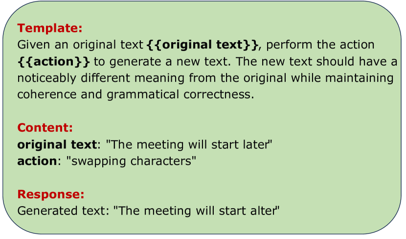
((a)) Character Swap

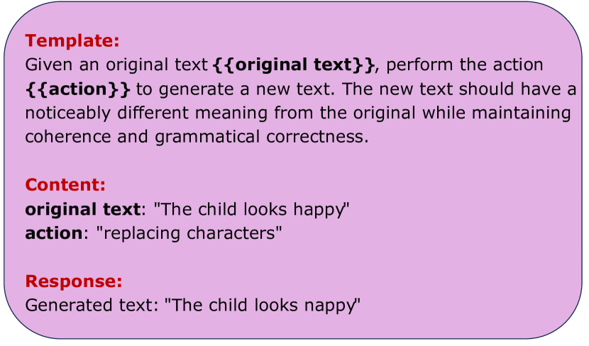
((b)) Character Replacement

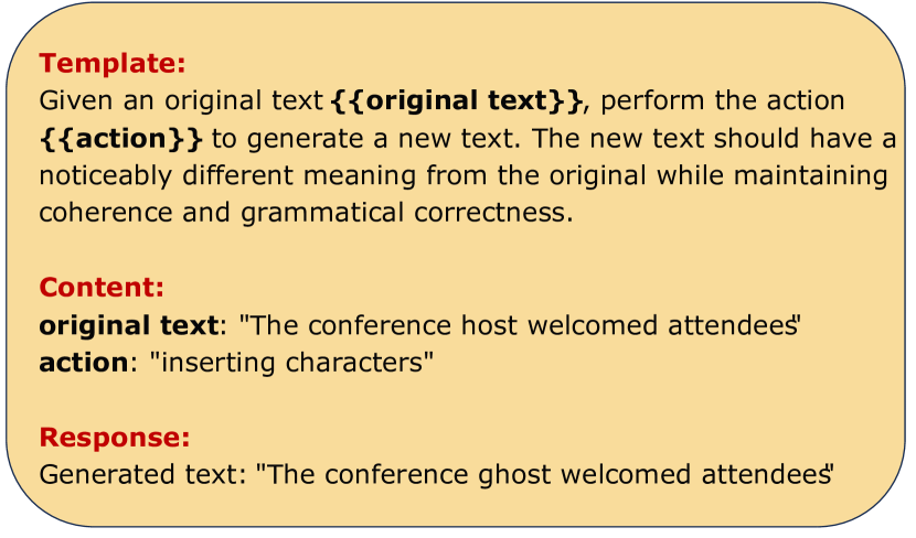
((c)) Character Insertion

Figure 1: Generation of perturbed texts via auxiliary LLM.

3 Methodology

3.1 Text Perturbation

Text perturbation is a data augmentation technique Guerrero et al. (2023) that introduces variability into textual data by applying a suite of carefully designed transformations to the original text samples.

Drawing on adversarial training principles Ganin et al. (2015), we design text perturbations that induce radical semantic shifts while preserving grammatical correctness. Through LLM-powered prompt templates (Figure 1), we propose three methods to generate perturbed text samples that systematically challenge model robustness:

3.1.1 Character Swap

• Example: Swapping “l” and “a” in “later” yields “alter”. The sentence “The meeting will start later” becomes “The meeting will start alter”.

• Impact: In scheduling systems, they erroneously generate rescheduling forms (e.g., ”Specify how to alter the meeting”) instead of directly acknowledging delays, causing workflow disruptions in calendar management tools. This error propagates further in Q&A systems, where models respond to timing-related queries with operational directives like ”How to adjust the meeting?” rather than factual acknowledgments, thereby disseminating incorrect procedural guidance to end-users and amplifying systemic inefficiencies.

3.1.2 Character Replacement

• Example: Replacing “h” with “n” in “happy” yields “nappy”. The sentence “The child looks happy” becomes “The child looks nappy”.

• Impact: In dialogue systems, they inappropriately suggest practical actions like Check diaper supplies” instead of providing emotional support, resulting in nonsensical interactions within childcare applications. This confusion is compounded in healthcare chatbots, where models misinterpret phrases such as The patient feels nappy” as clinical symptoms (e.g., erroneously recommending diaper rash cream for skin irritation), thereby dispensing inappropriate medical advice and undermining trust in AI-driven systems.

3.1.3 Character Insertion

• Example: Inserting “g” to “host” yields “ghost”. The sentence “The conference host welcomed attendees” becomes “The conference ghost welcomed attendees”.

• Impact: In automated summarization, models may generate fictional narratives (e.g., “A paranormal event occurred during the conference”), thereby misrepresenting factual events and eroding trust in reporting systems. In enterprise search, models may retrieve irrelevant documents (e.g., entertainment media) instead of relevant conference records, introducing noise into enterprise knowledge graphs and decision-making pipelines.

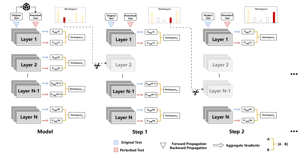
Figure 2: Overview of our PIP method, where an auxiliary LLM generates perturbed text (see Section 3.1). During pruning, the same original and perturbed texts are used to compute PertImport values, determining layer significance. The least significant layers (e.g., the 2nd, (N–1)-th, and N-th layers in the first three steps) are iteratively removed.

3.2 PertImport: A Perturbation-based Metric for Layer Importance Assessment

Building on the text perturbation framework defined in Section 3.1, we propose PertImport, a novel metric to measure the sensitivity to meaning-altering inputs. The rationale for this metric is grounded in the following analysis:

Consider a pre-trained large language model $\mathcal{M}$ with $N$ layers. Each layer $i$ has parameters $\mathbf{w}_{i}\in\mathbb{R}^{n}$. Excluding embedding and head layers, $\mathcal{M}$ can be seen as a mapping function $f$. For any input $s$, the function $f(s;\mathbf{w}_{1},\mathbf{w}_{2},\ldots,\mathbf{w}_{N})$ generates an output that is consistent with $s$’s semantics.

In Supervised Fine-Tuning (SFT) Brown et al. (2020), when sample $s$ is utilized as both input and label for model $\mathcal{M}$, the parameter update equation is derived as follows:

$$\mathbf{w}_{i}^{\prime}=\mathbf{w}_{i}-\alpha\cdot\nabla_{\mathbf{w}_{i}}\mathcal{L}(s;\mathbf{w}_{1},\mathbf{w}_{2},\ldots,\mathbf{w}_{N}).$$ (1)

Introducing perturbation $\delta s$ (detailed in Section 3.1) to $s$ gives the perturbed sample $s+\delta s$. Using it for SFT yields:

$$\mathbf{w}_{i}^{\prime\prime}=\mathbf{w}_{i}-\alpha\cdot\nabla_{\mathbf{w}_{i}}\mathcal{L}(s+\delta s;\mathbf{w}_{1},\mathbf{w}_{2},\ldots,\mathbf{w}_{N}).$$ (2)

Here, $\mathbf{w}_{i}\in\mathbb{R}^{n}$ denotes the original parameters of the $i$-th layer, $\mathbf{w}_{i}^{{}^{\prime}}\in\mathbb{R}^{n}$ and $\mathbf{w}_{i}^{{}^{\prime\prime}}\in\mathbb{R}^{n}$ denote the updated parameters of the $i$-th layer, $\alpha$ is the learning rate, and the loss function $\mathcal{L}(\cdot)$ quantifies the difference between predictions and labels.

Given that $f$ is differentiable and $\delta s\to\mathbf{0}$, we can use the Taylor expansion formula to derive the following equation:

$$f(s+\delta s;\mathbf{w}_{1}^{{}^{\prime\prime}},\mathbf{w}_{2}^{{}^{\prime\prime}},\ldots,\mathbf{w}_{N}^{{}^{\prime\prime}})-f(s;\mathbf{w}_{1}^{{}^{\prime}},\mathbf{w}_{2}^{{}^{\prime}},\ldots,\mathbf{w}_{N}^{{}^{\prime}})$$

$$\approx\nabla_{s}f\cdot\delta s+\sum_{i}\sum_{j}(\nabla_{\mathbf{w}^{{}^{\prime}}_{i}}f)_{j}\cdot(\mathbf{w}_{i}^{{}^{\prime\prime}}-\mathbf{w}_{i}^{{}^{\prime}})_{j},$$ (3)

where $(\nabla_{\mathbf{w}^{{}^{\prime}}_{i}}f)_{j}\in\mathbb{R}$ represents the $j$-th element of the gradient vector $\nabla_{\mathbf{w}^{{}^{\prime}}_{i}}f$ at the $i$-th layer, and $(\mathbf{w}_{i}^{{}^{\prime\prime}}-\mathbf{w}_{i}^{{}^{\prime}})_{j}\in\mathbb{R}$ represents the $j$-th element of the parameter difference $\mathbf{w}_{i}^{{}^{\prime\prime}}-\mathbf{w}_{i}^{{}^{\prime}}$ at the $i$-th layer.

Subsequently, we utilize Equation (3.2) to establish an upper bound for the estimation of the difference in output values with and without the perturbation $\delta s$. We introduce a constant sequence $\left\{C_{i}\right\}_{i=1}^{N}$ defined as $C_{i}=\underset{1\leq j\leq n}{max}\left|(\nabla_{\mathbf{w}^{{}^{\prime}}_{i}}f)_{j}\right|$. Incorporating Equations (1), (2), and (3.2), we arrive at:

$$\left|f(s+\delta s;\mathbf{w}_{1}^{{}^{\prime\prime}},\mathbf{w}_{2}^{{}^{\prime\prime}},\ldots,\mathbf{w}_{N}^{{}^{\prime\prime}})-f(s;\mathbf{w}_{1}^{{}^{\prime}},\mathbf{w}_{2}^{{}^{\prime}},\ldots,\mathbf{w}_{N}^{{}^{\prime}})\right|$$

$$\leq\left|\nabla_{s}f\cdot\delta s\right|+$$

$$+C\sum_{i}\sum_{j}\left|(\nabla_{\mathbf{w}_{i}}(\mathcal{L}(s+\delta s;\mathcal{W})-\mathcal{L}(s;\mathcal{W})))_{j}\right|,$$ (4)

where $C=\underset{1\leq i\leq N}{max}\left\{C_{i}\right\}$ represents the maximum value of the sequence $\left\{C_{i}\right\}$, and $\mathcal{W}$ represents all the parameters of $\mathcal{M}$.

Theorem 1.

To enhance the robustness of the pruned model (defined as its capability to distinguish between $s$ and $s+\delta s$), it’s best to select parameters with smaller gradient differences between the perturbed and unperturbed views.

Proof.

Let $\mathbf{Y}$ be a random variable representing the output difference with and without the perturbation $\delta s$. Consider removing the parameter at the $i_{0}$-th layer and the $j_{0}$-th position, i.e., $(\mathbf{w}_{i_{0}})_{j_{0}}$. Suppose there exists another parameter $(\mathbf{w}_{i_{0}^{{}^{\prime}}})_{j_{0}^{{}^{\prime}}}$ that has a smaller gradient difference and a higher average probability of detecting the difference between $s$ and $s+\delta s$. Assuming, without loss of generality, that $\mathbf{Y}$ follows a uniform distribution, pruning $(\mathbf{w}_{i_{0}})_{j_{0}}$ leads to the following equation for the expectation of $\mathbf{Y}_{\overline{{i_{0}},{j_{0}}}}$:

$$\frac{2}{C}\mathbb{E}[\mathbf{Y}_{\overline{{i_{0}},{j_{0}}}}]-\frac{1}{C}\left|\nabla_{s}f\cdot\delta s\right|$$

$$=\sum_{(i,j)\neq(i_{0},j_{0})}\left|(\nabla_{\mathbf{w}_{i}}(\mathcal{L}(s+\delta s;\mathcal{W})-\mathcal{L}(s;\mathcal{W})))_{j}\right|.$$ (5)

Similarly, when $(\mathbf{w}_{i_{0}^{{}^{\prime}}})_{j_{0}^{{}^{\prime}}}$ is pruned, we can derive the equation for the expectation of $\mathbf{Y}_{\overline{{i_{0}^{{}^{\prime}}},{j_{0}^{{}^{\prime}}}}}$ as follows:

$$\frac{2}{C}\mathbb{E}[\mathbf{Y}_{\overline{{i_{0}^{{}^{\prime}}},{j_{0}^{{}^{\prime}}}}}]-\frac{1}{C}\left|\nabla_{s}f\cdot\delta s\right|$$

$$=\sum_{(i,j)\neq(i_{0}^{{}^{\prime}},j_{0}^{{}^{\prime}})}\left|(\nabla_{\mathbf{w}_{i}}(\mathcal{L}(s+\delta s;\mathcal{W})-\mathcal{L}(s;\mathcal{W})))_{j}\right|.$$ (6)

By Equations (3.2) and (3.2), we have $\mathbb{E}[\mathbf{Y}_{\overline{{i_{0}},{j_{0}}}}]>\mathbb{E}[\mathbf{Y}_{\overline{{i_{0}^{{}^{\prime}}},{j_{0}^{{}^{\prime}}}}}]$, This finding contradicts the initial hypothesis that eliminating $(\mathbf{w}_{i_{0}^{{}^{\prime}}})_{j_{0}^{{}^{\prime}}}$ would increase the likelihood of detecting perturbation. Consequently, the assumption is invalid, implying that the theorem holds. ∎

Algorithm 1 Detailed Implementation of PIP Method

0: Pre-trained LLM $\mathcal{M}$; Calibration dataset $\mathcal{D}$; Text perturbation method $\delta(\cdot)$; Gradient aggregation function $g(\cdot)$; Number $L$ of layers to prune

0: Indices of the pruned layers $\mathcal{P}$; Pruned model $\mathcal{M}^{*}$

1: $\mathcal{D}^{{}^{\prime}}\leftarrow\delta(\mathcal{D});$

2: $\mathcal{M}^{*}\leftarrow\mathcal{M};$

3: $N_{\mathcal{M}}\leftarrow|\mathcal{M}.layers|;$

4: $\mathcal{P}\leftarrow\emptyset;$

5: for $\ell=1$ to $L$ do

6:  $\left\{\boldsymbol{G}_{agg}(i)\right\}_{i=1}^{N_{\mathcal{M}}-\ell+1}\leftarrow(g\circ SFT)(\mathcal{M}^{*},\mathcal{D});$

7:  $\left\{\boldsymbol{G^{\prime}}_{agg}(i)\right\}_{i=1}^{N_{\mathcal{M}}-\ell+1}\leftarrow(g\circ SFT)(\mathcal{M}^{*},\mathcal{D}^{{}^{\prime}});$

8:  $p_{\ell}\leftarrow{argmin}_{1\leq i\leq N_{\mathcal{M}}-\ell+1}|\boldsymbol{G}_{agg}(i)-\boldsymbol{G^{\prime}}_{agg}(i)|;$

9:  $\mathcal{P}\leftarrow\mathcal{P}\cup\left\{p_{\ell}\right\};$

10:  $\mathcal{M}^{*}\leftarrow\mathcal{M}^{*}\setminus\left\{layer_{p_{\ell}}\right\};$

11: end for

12: return $\mathcal{P}$, $\mathcal{M}^{*}$

Based on Theorem 1, we propose a robustness-aware importance metric, PertImport. For the $i$-th layer, PertImport quantifies its discriminative sensitivity through:

$$\frac{1}{|\mathcal{D}|}\sum_{s\in\mathcal{D}} |g((\nabla_{\mathbf{w}_{i}}\mathcal{L}(s+\delta s;\mathcal{W}))_{1},\ldots,(\nabla_{\mathbf{w}_{i}}\mathcal{L}(s+\delta s;\mathcal{W}))_{n})$$

$$- g((\nabla_{\mathbf{w}_{i}}\mathcal{L}(s;\mathcal{W}))_{1},\ldots,(\nabla_{\mathbf{w}_{i}}\mathcal{L}(s;\mathcal{W}))_{n})|,$$ (7)

where $\mathcal{D}$ is a small calibration dataset, and $n$ is the count of parameters in the $i$-th layer of $\mathcal{M}$. The function $g:\mathbb{R}^{n}\to\mathbb{R}$ aggregates gradient information for a specific layer using norms like $L_{1}$, $L_{2}$, or $L_{\infty}$, as shown in Han et al. (2015). For the definitions of these norms, please refer to Appendix A.

3.3 PIP: Perturbation-based Iterative Pruning

After assessing the importance of each layer through perturbation, we avoid prematurely determining the indices of all target layers to prune. Instead, we adopt a more systematic approach by employing an iterative greedy strategy. Specifically, PIP leverages a double-view perspective by comparing the gradient differences between the unperturbed view and the perturbed view to evaluate layer importance. This double-view approach enables PIP to iteratively identify and prune one layer at a time, ensuring minimal impact on performance.

By integrating information from these distinct views, PIP reduces the randomness inherent in the pruning process and ensures a more controlled and efficient optimization. The detailed implementation of PIP is presented in Algorithm 1, and the overall workflow is illustrated in Figure 2.

4 Experiments

4.1 Experimental Setup

4.1.1 Model Selection

To ensure a comprehensive comparison with a diverse range of existing approaches, we conduct experiments on a suite of LLMs that vary in size, specifically from the LLaMA2 Touvron et al. (2023) and LLaMA3 Dubey et al. (2024) series. The selection of these series is strategic, as they are widely recognized and utilized across various methodologies, thereby providing a robust and standardized platform for our comparative analysis.

4.1.2 Evaluation and Datasets

We use seven datasets to evaluate accuracy: BoolQClark et al. (2019), PIQABisk et al. (2020), HellaSwagZellers et al. (2019), WinoGrandeSakaguchi et al. (2021), ARC-EasyClark et al. (2018), ARC-ChallengeClark et al. (2018), and OpenBookQAMihaylov et al. (2018), all of which have been widely used in previous structured pruning studies. To ensure a fair comparison across the aforementioned datasets, we utilize the LM Evaluation Harness framework Gao et al. (2024) with its default settings for evaluation, without incorporating any shots as demonstrations. In addition, we evaluate perplexity (PPL) on the PTB datasetMarcus et al. (1993),to assess the capability of predicting the next token.

4.1.3 Baseline Methods

To show the effectiveness of PIP, we compare it with several state-of-the-art structured pruning methods for LLMs:

• LLM-Pruner Ma et al. (2023): A method which uses Taylor-based metrics to prune less important heads within the Multi-Head Attention mechanism and neurons within the Feed-Forward Network.

• SliceGPT Ashkboos et al. (2024): A method which applies orthogonal transformations to prune rows and columns of weight matrices, reducing the hidden size.

• ShortGPT Men et al. (2024): A method which identifies redundant layers that have a small similarity between the inputs and outputs, pruning those to reduce the depth.

To compare with baselines, we follow the same experiment settings suggested in their studies.

4.1.4 Experimental Details

Following Ashkboos et al. (2024), we randomly select a few samples (fewer than 10) from the WikiText2 dataset Merity et al. (2016) for calibration, using a fixed random seed. We aggregate gradients using the $L_{2}$-norm. To highlight the effectiveness of our proposed method, we set a lower pruning ratio for baseline methods compared to PIP. Experiments are conducted using the Transformers library Wolf (2020) on a server with 8 NVIDIA A100 GPUs (80GB VRAM each, totaling 640GB).

4.1.5 Statistics of Pruned Models

Table 1 summarises key characteristics of the pruned models utilized in our primary experiments, including parameter count, memory footprint, and Time-Per-Output-Token (TPOT). Evaluations use a randomly sampled sequence from WikiText2 with a fixed output length of 128 tokens. For hardware configuration: LLaMA2-8B and LLaMA3-13B are tested on a single NVIDIA A100 GPU, while LLaMA2-70B and LLaMA3-70B employ tensor parallelism across 4 NVIDIA A100 GPUs. All experiments are executed in half-precision (FP16) mode.

Model	Ratio	#Params	Memory	TPOT
LLaMA3-8B	Dense	8.0B	15.0GiB	46.7ms
	19.0%	6.5B	12.1GiB	41.5ms
LLaMA3-70B	Dense	70.6B	131.4GiB	266.2ms
	19.4%	56.9B	99.5GiB	223.5ms
LLaMA2-13B	Dense	13.0B	24.4GiB	73.4ms
	19.5%	10.5B	19.6GiB	58.9ms
LLaMA2-70B	Dense	69.0B	128.5GiB	269.7ms
	19.9%	55.3B	96.6GiB	217.8ms

Table 1: Statistics of base and pruned models. “Dense” denotes the original unpruned model. “Ratio” refers to the pruning ratio, which is calculated as $(\text{\#Pruned Params})/({\text{\#Base Params}})$.

Model	Method	PPL↓	BoolQ↑	PIQA↑	HeSwg↑	WGrd↑	ARC-E↑	ARC-C↑	OBQA↑	Avg.↑
LLaMA3-8B	Dense	10.6	81.4	79.7	60.2	72.5	80.1	50.5	34.8	65.6
	LLM-Pruner	56.5	63.5	69.5	42.6	62.4	52.3	29.5	27.0	49.5
	SliceGPT	72.3	40.8	65.4	39.8	63.2	59.5	29.4	23.8	46.0
	ShortGPT	67.9	65.2	68.9	45.6	69.4	57.2	36.5	25.4	52.6
	PIP (Ours)	56.3	70.9	69.6	44.7	69.4	57.9	35.1	26.8	53.5
LLaMA3-70B	Dense	8.2	85.2	82.4	66.4	80.3	86.9	60.3	38.2	71.4
	LLM-Pruner	-	-	-	-	-	-	-	-	-
	SliceGPT	78.2	59.4	69.6	44.4	72.1	69.7	41.1	30.2	55.2
	ShortGPT	13.9	80.9	76.0	57.1	60.5	77.4	47.9	19.0	59.8
	PIP (Ours)	12.5	79.0	78.6	56.1	73.3	75.7	45.3	29.6	62.5
LLaMA2-13B	Dense	28.9	80.6	79.1	60.0	72.4	79.4	48.5	35.2	65.0
	LLM-Pruner	150.2	57.7	60.3	31.9	53.9	37.4	22.9	15.8	40.1
	SliceGPT	64.3	38.2	65.0	39.5	65.5	61.3	33.4	28.0	47.3
	ShortGPT	44.6	49.8	55.5	39.3	57.1	49.3	29.9	25.4	43.8
	PIP (Ours)	41.8	63.3	74.5	50.5	62.0	58.8	37.4	25.0	53.1
LLaMA2-70B	Dense	14.4	76.6	81.1	64.0	77.0	77.8	51.2	34.8	66.1
	LLM-Pruner	-	-	-	-	-	-	-	-	-
	SliceGPT	33.9	70.1	76.3	52.7	76.6	76.4	47.0	32.6	61.7
	ShortGPT	18.5	73.5	73.9	56.0	72.5	66.7	39.2	26.8	58.4
	PIP (Ours)	17.2	80.7	77.0	57.8	73.4	70.7	43.6	29.4	61.8

Table 2: Zero-shot performance of LLMs with approximately 20% pruning ratio. “Dense” denotes the original unpruned model. Symbols “↑” (higher is better) and “↓” (lower is better) indicate metric directions. Bold values denote the best performance among pruned models, underlined values the second-best. Abbreviations: HellaSwag (HeSwg), WinoGrande (WGrd), ARC-Easy (ARC-E), ARC-Challenge (ARC-C), OpenBookQA (OBQA). “Avg.” represents the average score across the seven benchmarks. “-” indicates incompatibility between pruning methods and specific LLMs.

4.2 Zero-shot Performance

In this part, we conduct a comprehensive comparison of PIP against baselines regarding zero-shot performance. The detailed experimental results are presented in Table 2. On average, PIP retains over 85% of the Dense model’s accuracy over various benchmarks, with an approximate pruning ratio of 20%. In some cases, PIP’s performance is within a mere 5% range of the Dense model’s scores, highlighting its ability to preserve crucial aspects of the Dense model’s effectiveness. This level of performance retention positions PIP as a highly valuable approach for pruning LLMs without significant performance degradation. Furthermore, PIP consistently outperforms baseline methods, thereby further solidifying its status as a superior technique for pruning LLMs. For more details, readers are referred to Appendix C.

4.3 Ablation Analysis

To systematically investigate the critical components of our PIP pruning framework, we conduct ablation studies on LLaMA2-13B focusing on two core mechanisms: perturbation and greedy-search iteration. As shown in Table 3, we evaluate three progressive pruning ratios (9.8%, 19.5%, 29.2%) under three experimental configurations: (1) Full PIP implementation, (2) Perturbation-only, and (3) Iteration-only. The performance is measured using the PPL metric on the PTB dataset.

Our findings indicate that perturbation and iteration synergistically enhance pruning efficacy. At a 29.2% pruning ratio, the combined approach (Perturbation: 2714, Iteration: 2714) achieves optimal performance (PPL=53.3), while disabling iteration (Perturbation: 2714, Iteration: 2718) degrades performance by 26.5% (PPL=67.4). Additionally, the absence of perturbation (Perturbation: 2718, Iteration: 2714) causes more severe deterioration (PPL=99.8), indicating perturbation’s critical role. Similar trends are observed at lower pruning ratios, where the combination of perturbation and iteration consistently outperforms their individual effects. This pattern persists across lower pruning ratios, confirming that the interaction between perturbation and iterative refinement mechanisms is essential for effective model compression.

Ratio	Perturbation	Iteration	PPL↓
9.8%	2714	2714	30.7
	2714	2718	31.3
	2718	2714	43.4
19.5%	2714	2714	41.8
	2714	2718	42.0
	2718	2714	81.9
29.2%	2714	2714	53.3
	2714	2718	67.4
	2718	2714	99.8

Table 3: Ablation studies of LLaMA2-13B. “Ratio”: Pruning Ratio; “2714”: Enabled; “2718”: Disabled.

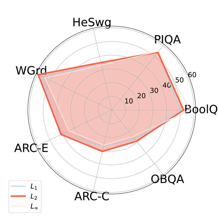
((a)) LLaMA3

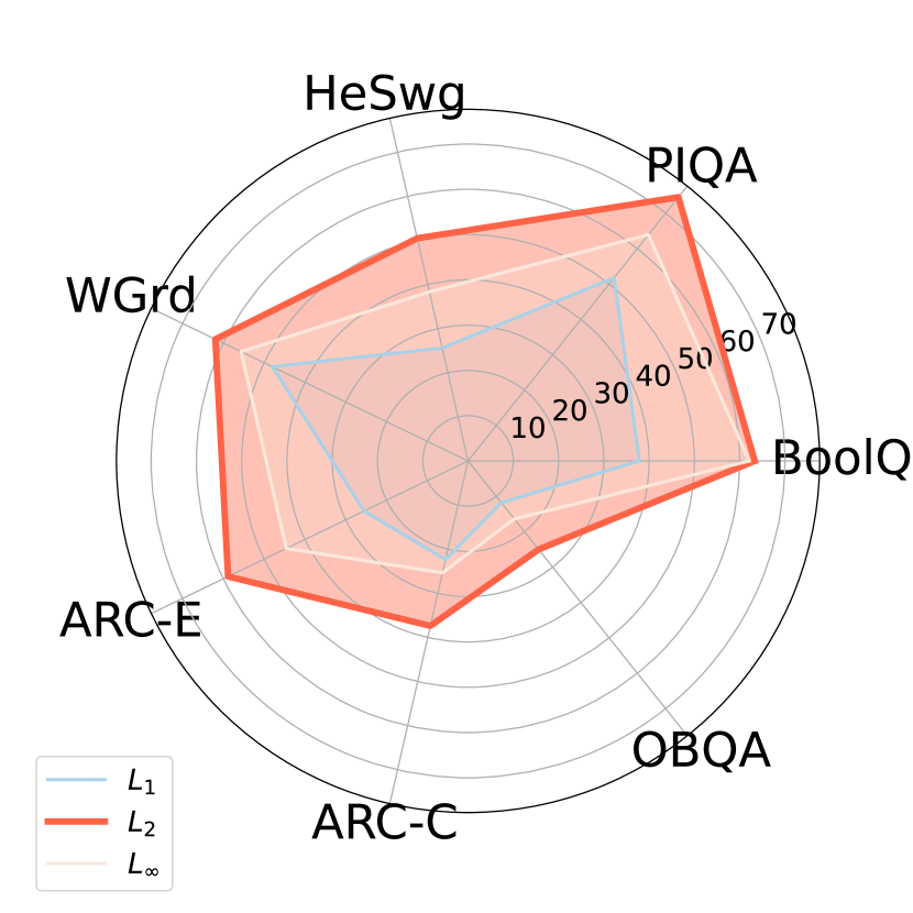
((b)) LLaMA2

Figure 3: Zero-shot performance of the pruned LLM using our PIP method, across various gradient aggregation strategies.

4.4 More Analysis

4.4.1 Impact of Gradient Aggregation

In this section, we explore the impact of employing different gradient aggregation strategies when pruning the model, as depicted in Figure 3. Overall, aggregating gradients via the $L_{2}$-norm tends to offer more advantages compared to the $L_{1}$ and $L_{\infty}$ norms. Unlike these other norms, the $L_{2}$-norm assigns more weight to larger gradients but does so in a controlled and balanced manner. This helps mitigate the influence of extreme gradient values while still enabling the PIP method to leverage gradients on a global scale. For more details, readers are referred to Appendix D.1.

4.4.2 Impact of Calibration Data Volume

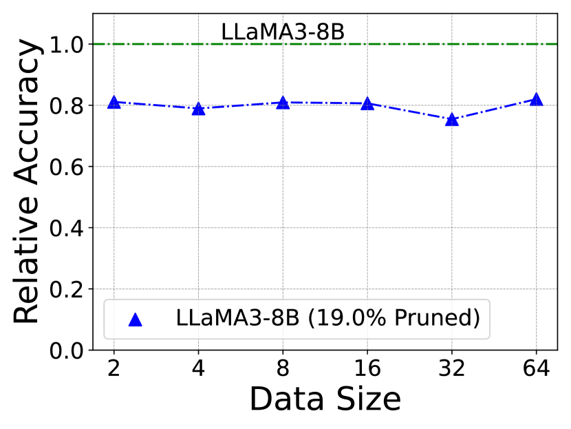
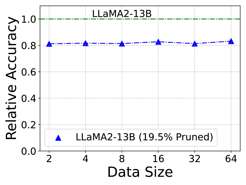
Figure 4: Experiments of performance at various data sizes. “Data Size” refers to the number of samples in the calibration dataset. “Relative Accuracy” denotes the ratio of the average accuracy of the pruned LLM on various benchmarks to the average accuracy of the Dense model.

In this section, we investigate how different volumes of calibration data influence the LLMs’ zero-shot performance after applying the PIP method. Specifically, we employ character swap and replacement techniques in conjunction with the $L_{2}$-norm for gradient aggregation.

As depicted in Figure 4, the PIP method exhibits remarkable efficiency in pruning with a minimal number of calibration samples, a concept referred to as “few-shot” learning. This characteristic is particularly beneficial, as it suggests that PIP can attain high performance without the necessity for an extensive dataset, thereby addressing a common limitation encountered in practical computational science applications. For more details, readers are referred to Appendix D.2.

4.4.3 Pruning Time Analysis

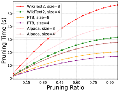
Figure 5: Impact of pruning ratio on pruning time.

Let the average time for forward propagation in a layer be $t_{f}$, and backward propagation be $t_{b}$. Using the PIP method, the time required to prune $m$ layers of model $\mathcal{M}$ is denoted as $PT_{\mathcal{M}}(m)$. The second finite difference of pruning time is calculated as follows:

$$\triangle^{2}PT_{\mathcal{M}}(m)=-(t_{f}+t_{b}),$$ (8)

where $\triangle^{2}$ denotes the second finite difference. This result implies constant second differences in $PT_{\mathcal{M}}(m)$, a hallmark of quadratic sequences. For a detailed proof, readers are referred to Appendix B.

Since the pruning ratio is proportional to $m$ (the number of pruned layers), the pruning time varies quadratically with respect to the pruning ratio. This aligns with empirical observations in Figure 5, where the PIP pruning time for the LLaMA3-8B model exhibits quadratic scaling across datasets and sample sizes (corresponding to the left side of the axis of symmetry in its quadratic relationship).

4.4.4 Generations from Pruned Models

The examples in Table 4 clearly demonstrate that the pruned LLMs, despite undergoing the PIP pruning method, retain robust language expression capabilities. For instance, the pruned LLaMA3 model is capable of generating a coherent and insightful statement about the impact of AI on the business world, highlighting its potential to change the future of work. Similarly, the pruned LLaMA2 model provides a comprehensive introduction to NLP, emphasizing its role in processing human languages and extracting valuable insights from unstructured text data. These examples validate our pruning methodology’s effectiveness in preserving core linguistic competencies, particularly in: technical semantic preservation, syntactic coherence across multi-clause constructions, and domain-appropriate register consistency. For more details, readers are referred to Appendix E.

Model	✂	Example
LLaMA3	2718	AI will be widely used in all areas of business, says Bjarne Corydon. The minister of business and growth, Bjarne Corydon is excited about what AI is doing to the Danish business world.
	2714	AI will change the world of work: this is what the Gartner report reveals. In the coming years, AI will have a large impact on the entire business, as well as the daily life of employees.
LLaMA2	2718	NLP is a way of applying computational processing to natural human languages that we use to communicate with each other. This course will give you an introduction to NLP, and how it can be leveraged to derive useful insights from unstructured text data.
	2714	NLP is the science that focuses on linguistic data. It is an AI methodology that combines computer science and artificial intelligence. This science focuses on linguistic input, output, understanding, processing, or interaction. It is used to process human languages.

Table 4: Examples generated by the original model and the pruned model. “✂” indicates whether it is pruned. The underline highlights the prompt provided to the LLM.

5 Conclusion and Future Work

In this paper, we propose PIP, an innovative perturbation-based iterative structured pruning method that systematically unifies unperturbed and perturbed model views. Theoretical analysis confirms its robustness, while experiments demonstrate SOTA performance across multiple benchmarks.

For future research, it would be interesting to explore adaptive perturbation mechanisms (e.g., dynamically scaled or task-aware perturbations) to refine pruning granularity, and integration of domain-specific priors to enhance structured pruning. In addition, we aim to collaborate with industry partners to deploy PIP in real-world applications, such as edge computing systems, to validate its practical effectiveness and address any potential issues that may arise in actual scenarios.

Appendix A Definition of Norm

In this section, we provide the formal definitions of the norms used in the main text, specifically the $L_{1}$, $L_{2}$, and $L_{\infty}$ norms. These norms are commonly used in various mathematical and computational contexts to measure the magnitude of vectors.

A.1 $L_{1}$-norm

For a vector $\mathbf{x}=(x_{1},x_{2},\ldots,x_{n})\in\mathbb{R}^{n}$, the $L_{1}$-norm (also known as the Manhattan norm or Taxicab norm) is defined as:

$$\|\mathbf{x}\|_{1}=\sum_{i=1}^{n}|x_{i}|.$$ (9)

This norm represents the sum of the absolute values of the vector components.

A.2 $L_{2}$-norm

The $L_{2}$-norm (also known as the Euclidean norm) is perhaps the most commonly used norm. For a vector $\mathbf{x}=(x_{1},x_{2},\ldots,x_{n})\in\mathbb{R}^{n}$, it is defined as:

$$\|\mathbf{x}\|_{2}=\sqrt{\sum_{i=1}^{n}x_{i}^{2}}.$$ (10)

This norm represents the Euclidean length of the vector, which is the geometric distance from the origin to the point represented by the vector in $n$-dimensional space.

A.3 $L_{\infty}$-norm

The $L_{\infty}$-norm (also known as the maximum norm or infinity norm) is defined as:

$$\|\mathbf{x}\|_{\infty}=\max_{i}|x_{i}|.$$ (11)

This norm represents the maximum absolute value among the vector components.

Appendix B Proof of Constant Second Differences

We prove that if the second finite difference of pruning time satisfies $\triangle^{2}PT_{\mathcal{M}}(m)=-(t_{f}+t_{b})$ for all $m$, then $PT_{\mathcal{M}}(m)$ must be a quadratic sequence.

Proof.

Let $\triangle^{2}PT_{\mathcal{M}}(m)\equiv-(t_{f}+t_{b})$ be constant. By definition of finite differences, the second difference is the difference of consecutive first differences:

$$\triangle PT_{\mathcal{M}}(m+1)-\triangle PT_{\mathcal{M}}(m)=-(t_{f}+t_{b}).$$ (12)

This implies that the first differences $\triangle PT_{\mathcal{M}}(m)$ form an arithmetic sequence with common difference $-(t_{f}+t_{b})$. Explicitly, for initial first difference $\triangle PT_{\mathcal{M}}(0)$, we have:

$$\triangle PT_{\mathcal{M}}(m) =\triangle PT_{\mathcal{M}}(0)-(t_{f}+t_{b})m.$$ (13)

The pruning time $PT_{\mathcal{M}}(m)$ is then the cumulative sum of these first differences:

$$PT_{\mathcal{M}}(m) =PT_{\mathcal{M}}(0)+\sum_{k=0}^{m-1}\triangle PT_{\mathcal{M}}(k)$$

$$=PT_{\mathcal{M}}(0)+\sum_{k=0}^{m-1}\left[\triangle PT_{\mathcal{M}}(0)-(t_{f}+t_{b})k\right]$$

$$=PT_{\mathcal{M}}(0)+m\triangle PT_{\mathcal{M}}(0)-(t_{f}+t_{b})\frac{m(m-1)}{2}.$$ (14)

Letting $a\equiv-\frac{t_{f}+t_{b}}{2}$, $b\equiv\triangle PT_{\mathcal{M}}(0)+\frac{t_{f}+t_{b}}{2}$, and $c\equiv PT_{\mathcal{M}}(0)$, this simplifies to:

$$PT_{\mathcal{M}}(m) =am^{2}+bm+c,$$ (15)

which is explicitly a quadratic function of $m$. ∎

Model	Ratio	Pruned Layers
LLaMA3-8B	19.0%	22, 18, 23, 28, 19, 21, 27
LLaMA3-70B	19.4%	06, 11, 46, 50, 75, 34, 49, 04,
		20, 25, 48, 57, 60, 56, 55, 58
LLaMA2-13B	19.5%	36, 31, 28, 13, 35, 25, 38, 23
LLaMA2-70B	19.9%	59, 29, 67, 26, 60, 61, 50, 43,
		58, 57, 31, 17, 56, 74, 62, 49

Table 5: Pruned Models by PIP method in our main experiments.

Appendix C The Main Experiment

Our core experiments validate the PIP methodology across four model scales (8B-70B parameters), and the pruned models are presented in Table 5. All configurations employ less than 10 calibration samples from WikiText2, using $L_{2}$-norm gradient aggregation strategy.

Appendix D More Analysis

D.1 Impact of Gradient Aggregation

We systematically evaluate gradient aggregation norms ($L_{1}$, $L_{2}$, $L_{\infty}$) across model architectures under controlled pruning settings. The LLaMA3-8B experiments employ 8 calibration samples with character swap perturbation and 7-layer pruning, while LLaMA2-13B utilizes 4 samples with character replacement perturbation and 8-layer pruning. Table 6 presents the zero-shot benchmark results under various gradient aggregation strategies.

D.2 Impact of Calibration Data Volume

For LLaMA3-8B, experiments use WikiText2 as the calibration dataset. Layer importance scores are computed through $L_{2}$-norm aggregation of gradients, computing layer importance via $L_{2}$-norm aggregation of gradients under character swap perturbation. The LLaMA2-13B configuration maintains the $L_{2}$-norm aggregation and dataset while employing character-replacement perturbation. The complete lists of pruned layers (0-indexed) under each condition are provided in Table 7.

D.3 Impact of Pruning Ratio

We systematically evaluate the performance degradation of LLaMA3 and LLaMA2 models under increasing pruning ratios (10%–30%), as detailed in Table 8. As pruning ratios rise (10%→30%), both LLaMA3 and LLaMA2 show sharp performance drops. Commonsense tasks (ARC-Challenge, OBQA) decline the most, while language tasks (BoolQ, WinoGrande) are more robust.

D.4 Impact of Text Perturbation Method

The experiments are conducted on LLaMA3-8B under three text perturbation methods (Swap, Replace, Insert) with fixed configurations: 4 calibration samples, $L_{2}$-norm gradient aggregation. Table 9 compares the zero-shot performance across various benchmarks under different text perturbation methods. All perturbation methods degrade LLaMA3’s zero-shot performance, with Replace showing the least decline.

D.5 Impact of Calibration Dataset

The experiments evaluate the LLaMA3-8B model under three calibration datasets (WikiText2, PTB, Alpaca) with fixed configurations: 8 calibration samples, swap-based text perturbation, $L_{2}$-norm gradient aggregation. As presented in Table 10, PIQA and WinoGrande exhibit dataset-agnostic stability, whereas ARC-Challenge declines sharply under PTB.

Appendix E Generations from Pruned Models

Tables 11 and 12 demonstrate that models pruned via the PIP method retain text generation quality comparable to their dense counterparts. Pruned models preserve logical coherence and domain-specific knowledge (e.g., technical terminology and contextual reasoning), with minimal degradation in fluency and factual accuracy, validating PIP’s capability to identify and retain critical layers.

Model	Norm	Pruned Layers	BoolQ↑	PIQA↑	HeSwg↑	WGrd↑	ARC-E↑	ARC-C↑	OBQA↑	Avg.↑
LLaMA3	Dense	–	81.4	79.7	60.2	72.5	80.1	50.5	34.8	65.6
	$L_{1}$	23, 18, 29, 22, 11, 17, 10	49.8	54.1	33.7	57.1	41.5	27.0	27.4	41.5
	$L_{2}$	23, 22, 18, 19, 28, 20, 31	52.3	53.8	35.5	59.4	41.0	30.9	29.0	43.1
	$L_{\infty}$	20, 13, 18, 23, 12, 28, 22	56.9	54.9	33.6	54.1	34.7	26.3	24.8	40.7
LLaMA2	Dense	–	80.6	79.1	60.0	72.4	79.4	48.5	35.2	65.0
	$L_{1}$	00, 34, 35, 09, 12, 27, 10, 33	37.9	51.7	25.6	48.0	25.5	22.4	11.8	31.8
	$L_{2}$	36, 31, 28, 13, 35, 25, 38, 23	63.3	74.5	50.5	62.0	58.8	37.4	25.0	53.1
	$L_{\infty}$	30, 27, 24, 03, 28, 29, 17, 13	62.1	63.9	38.3	55.6	44.6	25.3	16.4	43.8

Table 6: Zero-shot performance comparison across different gradient aggregation strategies.

Model	Cnt.	Pruned Layers	BoolQ↑	PIQA↑	HeSwg↑	WGrd↑	ARC-E↑	ARC-C↑	OBQA↑	Avg.↑
LLaMA3	Dense	–	81.4	79.7	60.2	72.5	80.1	50.5	34.8	65.6
	2	23, 22, 18, 30, 25, 27, 26	74.0	68.7	42.8	68.9	57.7	34.9	25.4	53.2
	4	31, 22, 24, 25, 30, 28, 07	62.3	70.1	41.8	61.2	61.8	37.1	28.4	51.8
	8	23, 18, 22, 19, 28, 21, 20	76.0	69.1	44.5	67.1	55.7	34.4	24.8	53.1
	16	23, 31, 24, 21, 25, 22, 18	70.5	68.4	45.5	63.6	56.7	38.3	27.4	52.9
	32	31, 30, 22, 10, 05, 17, 21	65.9	68.0	40.1	59.7	56.3	31.3	25.4	49.5
	64	31, 25, 23, 22, 28, 24, 19	66.2	70.2	47.8	65.4	58.5	39.5	28.8	53.8
LLaMA2	Dense	–	80.6	79.1	60.0	72.4	79.4	48.5	35.2	65.0
	2	09, 25, 34, 21, 14, 19, 31, 06	62.5	73.9	49.0	60.7	65.2	32.7	25.4	52.8
	4	36, 31, 28, 13, 35, 25, 38, 23	63.3	74.5	50.5	62.0	58.8	37.4	25.0	53.1
	8	34, 36, 31, 21, 26, 22, 07, 05	64.8	73.0	50.3	64.1	60.4	33.8	24.2	52.9
	16	29, 08, 27, 30, 25, 35, 23, 17	62.4	74.0	51.6	64.3	60.9	37.3	26.0	53.8
	32	31, 33, 17, 23, 32, 19, 16, 14	69.4	73.8	49.9	62.1	57.2	31.9	25.8	52.9
	64	36, 33, 17, 30, 24, 27, 13, 31	62.8	74.4	52.4	63.5	61.7	36.9	27.0	54.1

Table 7: Zero-shot performance comparison across different numbers of calibration samples. “Cnt.”: the number of calibration samples.

Model	Ratio	Pruned Layers	BoolQ↑	PIQA↑	HeSwg↑	WGrd↑	ARC-E↑	ARC-C↑	OBQA↑	Avg.↑
LLaMA3	Dense	–	81.4	79.7	60.2	72.5	80.1	50.5	34.8	65.6
	10.9%	22, 18, 23, 28	78.8	75.2	53.2	72.8	71.0	43.3	29.4	60.5
	19.0%	22, 18, 23, 28, 19, 21, 27	70.9	69.6	44.7	69.4	57.9	35.1	26.8	53.5
	29.9%	22, 18, 23, 28, 19, 21, 27, 10,	43.5	63.0	36.4	56.2	43.3	30.0	25.0	42.5
		25, 06, 31
LLaMA2	Dense	–	80.6	79.1	60.0	72.4	79.4	48.5	35.2	65.0
	9.8%	36, 31, 28, 13	63.0	76.1	56.0	66.1	67.4	41.6	30.4	57.2
	19.5%	36, 31, 28, 13, 35, 25, 38, 23	63.3	74.5	50.5	62.0	58.8	37.4	25.0	53.1
	29.2%	36, 31, 28, 13, 35, 25, 38, 23,	62.4	71.3	45.9	58.4	46.9	33.9	23.8	48.9
		17, 26, 29, 30

Table 8: Zero-shot performance comparison across different pruning ratios. “Ratio” refers to the pruning ratio.

Model	TPM	Pruned Layers	BoolQ↑	PIQA↑	HeSwg↑	WGrd↑	ARC-E↑	ARC-C↑	OBQA↑	Avg.↑
LLaMA3	Dense	–	81.4	79.7	60.2	72.5	80.1	50.5	34.8	65.6
	Swap	23, 22, 31, 25, 16, 26, 30	63.9	69.5	44.7	63.6	58.7	36.0	31.2	52.5
	Replace	22, 18, 23, 28, 19, 21, 27	70.9	69.7	44.8	69.6	58.0	35.1	27.4	53.6
	Insert	23, 18, 31, 28, 22, 27, 03	71.3	70.2	47.6	64.4	57.8	36.3	25.0	53.2

Table 9: Zero-shot performance comparison across different text perturbation methods. “TPM”: Text Perturbation Method.

Model	CD	Pruned Layers	BoolQ↑	PIQA↑	HeSwg↑	WGrd↑	ARC-E↑	ARC-C↑	OBQA↑	Avg.↑
LLaMA3	Dense	–	81.4	79.7	60.2	72.5	80.1	50.5	34.8	65.6
	WikiText2	31, 28, 26, 29, 23, 25, 30	80.6	69.3	42.8	62.3	61.2	39.2	30.6	55.1
	PTB	23, 18, 28, 22, 19, 21, 13	72.1	70.6	44.6	66.6	54.8	32.9	24.0	52.2
	Alpaca	31, 30, 29, 28, 23, 25, 27	80.5	70.7	42.7	63.1	60.5	38.6	30.4	55.2

Table 10: Zero-shot performance comparison across different calibration datasets. “CD”: Calibration Dataset.

Model	✂	Example
LLaMA3	2718	Large Language Models will not replace us with AI – but they will help us automate our day-to-day work. AI has always been portrayed as the main reason behind replacing human labour with machine labour in many fields. For example, driverless cars and automated machines that replace employees are all examples of how AI will “replace” humans. However, AI has never replaced us, but has helped us automate many of our day-to-day operations and we will continue to see that trend of using AI in automation. One of the main reasons why AI has helped us improve our day-to-day work is that it is able to process, analyse and understand massive amounts of data. Large Language Models (LLMs) are a good example of this. LLMs can be a very useful tool to help us become more productive and improve our workflows. LLMs can also help us in many different ways, depending on what we are looking for, and they can be used in different ways. LLMs are able to process, analyse and understand massive amounts of text in many different ways. For example, they can be used to find information in a large amount of text, to do sentiment analysis, or to create new text. LLMs can also be used to do translation or to do a search in a large number of different languages. There are many tools available that allow us to work with LLMs, such as GPT-3 from OpenAI, which is one of the most powerful tools in the LLM space. LLMs can also be used to do sentiment analysis of text and we can use it in many different ways to help us become more productive and to improve our workflow. We can use LLMs to understand what is the sentiment of a large amount of text, to detect negative or positive sentiments in text, or to help us make decisions in our daily work. There are many ways to use LLMs to automate our day-to-day work. For example, we can use LLMs to help us become more productive and to improve our workflow by doing sentiment analysis. We can use LLMs to analyse large amounts of data and to analyse the sentiment of a large amount of text. We can use LLMs to help us find the right information in a large amount of text. We can use LLMs to translate text from one language to another, or to help us find the right information in a large amount of text.
	2714	Large Language Models will be the next killer apps. The way these LLMs are developed is not only more efficient but also very innovative in terms of how the LLMs are built, the use of compute to build the LLM, and how they train and generate LLMs. What’s more, we are seeing a change in how LLMs are used for tasks, with an increasing number of LLMs being used to train other AI models. This has opened up a huge market for LLMs, creating a great opportunity for companies like Cytora and Credence to tap into. In this article, we explore the benefits of this new wave of AI development, and how companies can capitalize on the opportunities presented by these new AI innovations. Large language models (LLMs) have been a focus of AI innovation for some time, and there are many ways they can be developed. However, the most effective and efficient way to develop LLMs is to use a lab environment that is specific to LLM development. There are two main approaches to developing LLMs: traditional computing methods, which require large amounts of computing power and data, and cloud-based LLMs, which can be developed much more quickly and inexpensively. There are several reasons why it is better to develop LLMs in an AI innovation lab than in a traditional development environment. First, the cloud-based LLM development process allows for much greater scale. With only a few machines in use, LLM developers can achieve huge breakthroughs, such as improving text generation accuracy. Second, cloud-based LLM development also allows for a much more nimble process. Instead of waiting for computers to complete tasks one at a time, developers can use a variety of machines to speed up their work. This speeds up the entire process, making it easier to get feedback from stakeholders and improving the overall experience of working with LLMs. How LLMs Can Be Used to Train Other AI Models. Large language models (LLMs) have been a driving force in the development of Artificial Intelligence (AI) over the years. These massive databases help to reduce the time it takes to train AI models, as well as reducing the energy consumption of these models. In addition, LLMs can be used to train other AI models, such as neural network models.

Table 11: Examples generated by the original model and the pruned model. “✂” indicates whether it is pruned. The underline highlights the prompt provided to the LLM.

Model	✂	Example
LLaMA2	2718	Large Language Models will be ubiquitous in business and government within 5-7 years, predicts PwC by James Sanders in Artificial Intelligence on January 30, 2023, 11:41 AM PST. Large Language Models such as OpenAIś GPT-3 are becoming increasingly prevalent for a wide variety of business applications, the consulting firm said. Image: Bjorn Rune Lie, Getty Images. The adoption rate of large language models—AI models trained on massive amounts of natural language data—will increase rapidly as businesses look to improve customer engagement and operational efficiencies. According to a report by PwC, 65% of senior business executives indicated that large language models are a top investment area, and 53% said that this is the largest investment area for AI technology in the coming year. ”Making AI more accessible, through advances such as large language models, is essential to the democratization of the technology, which could bring a range of business benefits to organizations,” said John Garner, global AI leader at PwC, in a statement accompanying the report. SEE: The ethical dilemmas of AI (ZDNET/TechRepublic special feature) — Download the free PDF version (TechRepublic) PwCś 2023 Global Artificial Intelligence Survey found that the use of natural language processing technologies is rapidly growing in the workplace. The technology is being used by 36% of respondents to ”identify risks or anomalies in client engagement,” and by 35% of respondents to ”increase the effectiveness and efficiency of operations.” AI is also used to drive productivity: 25% of respondents indicated that AI is used to ”enable the creation of new product and service offerings.” The growing ubiquity of large language models in the workplace is also a factor driving widespread awareness: 55% of business executives indicated that large language models are ”extremely important” to business success and operations, and 79% of employees said that they know of AI, a slight increase from last yearś survey. SEE: Large Language Models: What businesses need to know (ZDNET/TechRepublic special feature) — Download the free PDF version (TechRepublic) Most employees said that they would be comfortable working with systems powered by large language models: 56% indicated that they were comfortable in customer-facing roles, and 48% said that they were comfortable with large language models in back-end roles.
	2714	Large Language Models will be used for everything from translation to financial services to healthcare. There are endless benefits to utilizing LLMs like ChatGPT, like saving money and time on repetitive tasks that are time-consuming or impossible to automate, and getting better answers than we could on our own. As AI gets more accessible to average users, a more accessible education in AI is more important than ever. The ChatGPT revolution has arrived. If you are a regular user of Google search or Twitter, you’ve probably already noticed. ChatGPT was released to the public in November 2022 by an organization called OpenAI. The platform uses artificial intelligence to create intelligent chatbot responses to user prompts. As a result, it has the potential to revolutionize the way we interact with technology. With ChatGPT, you can write essays, do your taxes, and ask questions like “Who wrote Romeo and Juliet?” or “Where is the nearest Walmart?” in chat format. It’s accessible, fast, and most importantly, free. It’s clear that LLMs are a powerful tool with enormous applications and capabilities. But what, exactly, is an LLM, and why is this technology so different from other language models that have been developed? What Are Large Language Models? An LLM is a type of language modeling that produces language using machine learning algorithms based on large amounts of training data. It’s a relatively new development in the field of artificial intelligence, and it has become increasingly popular in recent years due to the advances in natural language processing and understanding that have been made. One of the main reasons for this is that large language models are capable of producing language that is more sophisticated and accurate than ever before. There are a few key reasons why large language models are different from other language models: They are based on very large amounts of data: This is the key characteristic that sets LLMs apart from other language models. Because of the amount of data used, these models can be trained to perform more complex tasks and generate more human-like text. They use a large number of parameters: The models also use a large number of parameters, which allows them to make more complex predictions about text. They are trained on a large number of tasks: The models are also trained on a large number of different tasks, which makes them more versatile than other language models.

Table 12: Examples generated by the original model and the pruned model. “✂” indicates whether it is pruned. The underline highlights the prompt provided to the LLM.

References

- Achiam et al. [2023] Josh Achiam, Steven Adler, Sandhini Agarwal, Lama Ahmad, Ilge Akkaya, Florencia Leoni Aleman, Diogo Almeida, Janko Altenschmidt, Sam Altman, Shyamal Anadkat, et al. Gpt-4 technical report. arXiv preprint arXiv:2303.08774, 2023.
- Ashkboos et al. [2024] Saleh Ashkboos, Maximilian L. Croci, Marcelo Gennari Do Nascimento, Torsten Hoefler, and James Hensman. Slicegpt: Compress large language models by deleting rows and columns. In The Twelfth International Conference on Learning Representations, ICLR 2024, Vienna, Austria, May 7-11, 2024. OpenReview.net, 2024.
- Bai et al. [2021] Haoli Bai, Wei Zhang, Lu Hou, Lifeng Shang, Jin Jin, Xin Jiang, Qun Liu, Michael Lyu, and Irwin King. BinaryBERT: Pushing the limit of BERT quantization. In Chengqing Zong, Fei Xia, Wenjie Li, and Roberto Navigli, editors, Proceedings of the 59th Annual Meeting of the Association for Computational Linguistics and the 11th International Joint Conference on Natural Language Processing (Volume 1: Long Papers), pages 4334–4348, Online, August 2021. Association for Computational Linguistics.
- Bisk et al. [2020] Yonatan Bisk, Rowan Zellers, Jianfeng Gao, Yejin Choi, et al. Piqa: Reasoning about physical commonsense in natural language. In Proceedings of the AAAI conference on artificial intelligence, volume 34, pages 7432–7439, 2020.
- Brown et al. [2020] Tom Brown, Benjamin Mann, Nick Ryder, Melanie Subbiah, Jared D Kaplan, Prafulla Dhariwal, Arvind Neelakantan, Pranav Shyam, Girish Sastry, Amanda Askell, et al. Language models are few-shot learners. Advances in neural information processing systems, 33:1877–1901, 2020.
- Clark et al. [2018] Peter Clark, Isaac Cowhey, Oren Etzioni, Tushar Khot, Ashish Sabharwal, Carissa Schoenick, and Oyvind Tafjord. Think you have solved question answering? try arc, the ai2 reasoning challenge. arXiv preprint arXiv:1803.05457, 2018.
- Clark et al. [2019] Christopher Clark, Kenton Lee, Ming-Wei Chang, Tom Kwiatkowski, Michael Collins, and Kristina Toutanova. Boolq: Exploring the surprising difficulty of natural yes/no questions. arXiv preprint arXiv:1905.10044, 2019.
- Davy [2024] Steven Davy. Tailored-llama: Optimizing few-shot learning in pruned llama models with task-specific prompts. In European Conference on Artificial Intelligence, 2024.
- Dubey et al. [2024] Abhimanyu Dubey, Abhinav Jauhri, Abhinav Pandey, Abhishek Kadian, Ahmad Al-Dahle, Aiesha Letman, Akhil Mathur, Alan Schelten, Amy Yang, Angela Fan, et al. The llama 3 herd of models. arXiv preprint arXiv:2407.21783, 2024.
- Fang et al. [2023] Gongfan Fang, Xinyin Ma, Mingli Song, Michael Bi Mi, and Xinchao Wang. Depgraph: Towards any structural pruning. In Proceedings of the IEEE/CVF conference on computer vision and pattern recognition, pages 16091–16101, 2023.
- Frantar and Alistarh [2023] Elias Frantar and Dan Alistarh. Sparsegpt: Massive language models can be accurately pruned in one-shot. In Andreas Krause, Emma Brunskill, Kyunghyun Cho, Barbara Engelhardt, Sivan Sabato, and Jonathan Scarlett, editors, International Conference on Machine Learning, ICML 2023, 23-29 July 2023, Honolulu, Hawaii, USA, volume 202 of Proceedings of Machine Learning Research, pages 10323–10337. PMLR, 2023.
- Ganin et al. [2015] Yaroslav Ganin, E. Ustinova, Hana Ajakan, Pascal Germain, H. Larochelle, François Laviolette, Mario Marchand, and Victor S. Lempitsky. Domain-adversarial training of neural networks. In Journal of machine learning research, 2015.
- Gao et al. [2024] Leo Gao, Jonathan Tow, Baber Abbasi, Stella Biderman, Sid Black, Anthony DiPofi, Charles Foster, Laurence Golding, Jeffrey Hsu, Alain Le Noac’h, Haonan Li, Kyle McDonell, Niklas Muennighoff, Chris Ociepa, Jason Phang, Laria Reynolds, Hailey Schoelkopf, Aviya Skowron, Lintang Sutawika, Eric Tang, Anish Thite, Ben Wang, Kevin Wang, and Andy Zou. A framework for few-shot language model evaluation, 07 2024.
- Guerrero et al. [2023] Jesus Guerrero, Gongbo Liang, and Izzat Alsmadi. Adversarial text perturbation generation and analysis. 2023 3rd Intelligent Cybersecurity Conference (ICSC), pages 67–73, 2023.
- Han et al. [2015] Song Han, Jeff Pool, John Tran, and William Dally. Learning both weights and connections for efficient neural network. Advances in neural information processing systems, 28, 2015.
- Hu et al. [2022] Edward J. Hu, Yelong Shen, Phillip Wallis, Zeyuan Allen-Zhu, Yuanzhi Li, Shean Wang, Lu Wang, and Weizhu Chen. Lora: Low-rank adaptation of large language models. In The Tenth International Conference on Learning Representations, ICLR 2022, Virtual Event, April 25-29, 2022. OpenReview.net, 2022.
- Kaplan et al. [2020] Jared Kaplan, Sam McCandlish, Tom Henighan, Tom B Brown, Benjamin Chess, Rewon Child, Scott Gray, Alec Radford, Jeffrey Wu, and Dario Amodei. Scaling laws for neural language models. arXiv preprint arXiv:2001.08361, 2020.
- Kim et al. [2024] Bo-Kyeong Kim, Geonmin Kim, Tae-Ho Kim, Thibault Castells, Shinkook Choi, Junho Shin, and Hyoung-Kyu Song. Shortened llama: A simple depth pruning for large language models. arXiv preprint arXiv:2402.02834, 11, 2024.
- Kwon et al. [2022] Woosuk Kwon, Sehoon Kim, Michael W Mahoney, Joseph Hassoun, Kurt Keutzer, and Amir Gholami. A fast post-training pruning framework for transformers. Advances in Neural Information Processing Systems, 35:24101–24116, 2022.
- Lin et al. [2024] Ji Lin, Jiaming Tang, Haotian Tang, Shang Yang, Wei-Ming Chen, Wei-Chen Wang, Guangxuan Xiao, Xingyu Dang, Chuang Gan, and Song Han. Awq: Activation-aware weight quantization for on-device llm compression and acceleration. In P. Gibbons, G. Pekhimenko, and C. De Sa, editors, Proceedings of Machine Learning and Systems, volume 6, pages 87–100, 2024.
- Ma et al. [2023] Xinyin Ma, Gongfan Fang, and Xinchao Wang. Llm-pruner: On the structural pruning of large language models. Advances in neural information processing systems, 36:21702–21720, 2023.
- Marcus et al. [1993] Mitch Marcus, Beatrice Santorini, and Mary Ann Marcinkiewicz. Building a large annotated corpus of english: The penn treebank. Computational linguistics, 19(2):313–330, 1993.
- Men et al. [2024] Xin Men, Mingyu Xu, Qingyu Zhang, Bingning Wang, Hongyu Lin, Yaojie Lu, Xianpei Han, and Weipeng Chen. Shortgpt: Layers in large language models are more redundant than you expect. arXiv preprint arXiv:2403.03853, 2024.
- Merity et al. [2016] Stephen Merity, Caiming Xiong, James Bradbury, and Richard Socher. Pointer sentinel mixture models, 2016.
- Mihaylov et al. [2018] Todor Mihaylov, Peter Clark, Tushar Khot, and Ashish Sabharwal. Can a suit of armor conduct electricity? a new dataset for open book question answering. In EMNLP, 2018.
- Pan et al. [2021] Haojie Pan, Chengyu Wang, Minghui Qiu, Yichang Zhang, Yaliang Li, and Jun Huang. Meta-KD: A meta knowledge distillation framework for language model compression across domains. In Chengqing Zong, Fei Xia, Wenjie Li, and Roberto Navigli, editors, Proceedings of the 59th Annual Meeting of the Association for Computational Linguistics and the 11th International Joint Conference on Natural Language Processing (Volume 1: Long Papers), pages 3026–3036, Online, August 2021. Association for Computational Linguistics.
- Saha et al. [2023] Rajarshi Saha, Varun Srivastava, and Mert Pilanci. Matrix compression via randomized low rank and low precision factorization. Advances in Neural Information Processing Systems, 36, 2023.
- Sakaguchi et al. [2021] Keisuke Sakaguchi, Ronan Le Bras, Chandra Bhagavatula, and Yejin Choi. Winogrande: An adversarial winograd schema challenge at scale. Communications of the ACM, 64(9):99–106, 2021.
- Song et al. [2024] Jiwon Song, Kyungseok Oh, Taesu Kim, Hyungjun Kim, Yulhwa Kim, and Jae-Joon Kim. SLEB: Streamlining LLMs through redundancy verification and elimination of transformer blocks. In Ruslan Salakhutdinov, Zico Kolter, Katherine Heller, Adrian Weller, Nuria Oliver, Jonathan Scarlett, and Felix Berkenkamp, editors, Proceedings of the 41st International Conference on Machine Learning, volume 235 of Proceedings of Machine Learning Research, pages 46136–46155. PMLR, 21–27 Jul 2024.
- Sun et al. [2020] Siqi Sun, Zhe Gan, Yuwei Fang, Yu Cheng, Shuohang Wang, and Jingjing Liu. Contrastive distillation on intermediate representations for language model compression. In Bonnie Webber, Trevor Cohn, Yulan He, and Yang Liu, editors, Proceedings of the 2020 Conference on Empirical Methods in Natural Language Processing (EMNLP), pages 498–508, Online, November 2020. Association for Computational Linguistics.
- Sun et al. [2024] Mingjie Sun, Zhuang Liu, Anna Bair, and J. Zico Kolter. A simple and effective pruning approach for large language models. In The Twelfth International Conference on Learning Representations, ICLR 2024, Vienna, Austria, May 7-11, 2024. OpenReview.net, 2024.
- Touvron et al. [2023] Hugo Touvron, Louis Martin, Kevin Stone, Peter Albert, Amjad Almahairi, Yasmine Babaei, Nikolay Bashlykov, Soumya Batra, Prajjwal Bhargava, Shruti Bhosale, et al. Llama 2: Open foundation and fine-tuned chat models. arXiv preprint arXiv:2307.09288, 2023.
- Vaswani [2017] A Vaswani. Attention is all you need. Advances in Neural Information Processing Systems, 2017.
- Wang et al. [2020] Ziheng Wang, Jeremy Wohlwend, and Tao Lei. Structured pruning of large language models. In Bonnie Webber, Trevor Cohn, Yulan He, and Yang Liu, editors, Proceedings of the 2020 Conference on Empirical Methods in Natural Language Processing, EMNLP 2020, Online, November 16-20, 2020, pages 6151–6162. Association for Computational Linguistics, 2020.
- Wolf [2020] Thomas Wolf. Transformers: State-of-the-art natural language processing. arXiv preprint arXiv:1910.03771, 2020.
- Xia et al. [2022] Mengzhou Xia, Zexuan Zhong, and Danqi Chen. Structured pruning learns compact and accurate models. In Smaranda Muresan, Preslav Nakov, and Aline Villavicencio, editors, Proceedings of the 60th Annual Meeting of the Association for Computational Linguistics (Volume 1: Long Papers), ACL 2022, Dublin, Ireland, May 22-27, 2022, pages 1513–1528. Association for Computational Linguistics, 2022.
- Xia et al. [2024] Mengzhou Xia, Tianyu Gao, Zhiyuan Zeng, and Danqi Chen. Sheared llama: Accelerating language model pre-training via structured pruning. In The Twelfth International Conference on Learning Representations, ICLR 2024, Vienna, Austria, May 7-11, 2024. OpenReview.net, 2024.
- Yuan et al. [2023] Zhihang Yuan, Yuzhang Shang, Yue Song, Qiang Wu, Yan Yan, and Guangyu Sun. Asvd: Activation-aware singular value decomposition for compressing large language models. arXiv preprint arXiv:2312.05821, 2023.
- Zellers et al. [2019] Rowan Zellers, Ari Holtzman, Yonatan Bisk, Ali Farhadi, and Yejin Choi. Hellaswag: Can a machine really finish your sentence? arXiv preprint arXiv:1905.07830, 2019.