Into the Void: Mapping the Unseen Gaps in High Dimensional Data

Abstract

We present a comprehensive pipeline, augmented by a visual analytics system named “GapMiner”, that is aimed at exploring and exploiting untapped opportunities within the empty areas of high-dimensional datasets. Our approach begins with an initial dataset and then uses a novel Empty Space Search Algorithm (ESA) to identify the center points of these uncharted voids, which are regarded as reservoirs containing potentially valuable novel configurations. Initially, this process is guided by user interactions facilitated by GapMiner. GapMiner visualizes the Empty Space Configurations (ESC) identified by the search within the context of the data, enabling domain experts to explore and adjust ESCs using a linked parallel-coordinate display. These interactions enhance the dataset and contribute to the iterative training of a connected deep neural network (DNN). As the DNN trains, it gradually assumes the task of identifying high-potential ESCs, diminishing the need for direct user involvement. Ultimately, once the DNN achieves adequate accuracy, it autonomously guides the exploration of optimal configurations by predicting performance and refining configurations, using a combination of gradient ascent and improved empty-space searches. Domain users were actively engaged throughout the development of our system. Our findings demonstrate that our methodology consistently produces substantially superior novel configurations compared to conventional randomization-based methods. We illustrate the effectiveness of our method through several case studies addressing various objectives, including parameter optimization, adversarial learning, and reinforcement learning.

I Introduction

THIS paper focuses on a methodology for effectively discovering “empty spaces”—regions where data points are absent—in multivariate and high-dimensional datasets. Identifying and exploring these empty spaces is both a challenge and an opportunity. The challenge is rooted in the curse of dimensionality, which is the exponential increase in volume and data sparsity associated with adding dimensions [5]. It makes the search for meaningful empty spaces increasingly complex, even for just a moderate number of attributes parameterizing the data.

Overcoming this complexity is not merely academic. It directly impacts the practicality of discovering and verifying new, unknown, and yet unimagined configurations that might reside within these empty spaces. Advocating for a configuration-discovery technique that can explore unconventional or even radical changes brought by unknown configurations and parameter settings offers a powerful alternative to conventional parameter tuning and optimization. These tasks are increasingly recognized as high priorities across diverse fields, including aerospace engineering [9], manufacturing [16], computer systems [2], personalized healthcare [63], and others, where techniques of this sort often address optimization problems with multiple objectives.

The emergence of crossover cars and hybrid vehicles illustrates well the high potential of exploring large parameter spaces to discover unique and unexpected configurations. Crossovers blend features from different vehicle types, offering drivers the versatility of an SUV with the agility of a sedan. Similarly, hybrids integrate gasoline engines with electric motors, improving fuel efficiency and reducing emissions without sacrificing performance. These examples demonstrate how investigating gaps within extensive parameter spaces can challenge conventional design constraints and embrace unconventional configurations. Clearly, innovation of this sort can also occur in lesser contexts.

While ingenious configurations become obvious once discovered, there are a multitude of them that defy practicality. Also, more often than not, high cost and substantial effort are required to obtain or simulate a hypothesized configuration to verify its merit. A human expert is often the best judge to decide whether to take up the risk of engaging in such a testing effort at all. But even with the human in the loop, the challenge lies in ideating meritorious configurations in the presence of this massive realm of possibilities.

To illustrate this challenge, consider a 4-dimensional parameter space with 50 levels for each dimension. This results in $50^{4}=$ 6.25 million possible configurations. Suppose we have data on the merit of 10,000 configurations from previous experiments. This means we have information on only 10,000/6,250,000 = 0.16% of the parameter space. While it is impractical to expect valid data at every location of the parameter space, the challenge lies in identifying which configurations are most useful. This uncertainty underscores the importance of intelligent sampling and discovery techniques to uncover valuable and innovative solutions.

While AI holds promise to replace human experts in this search, it requires ample high-quality training data to be effective. Our research supports this role of AI. Inspired by human-in-the-loop (HITL) [45] machine learning, our pipeline integrates the training of a deep neural network that evolves alongside the exploration process. This network aids in evaluating identified configurations and improves with accumulated data, enhancing search efficiency for verifying new configurations.

Conceptually, our method looks for gaps in high-D data spaces. While in theory the pairwise distances among data points in high-D space tend to be normally distributed with small variance, in practice, however, data configurations aggregate into hubs—points that occur more often in k-neighborhoods of nearby points than others [66]. Likewise, there are also anti-hubs—points that are unusually far away from most other points [50]. When these points exist, they are referred to as outliers, hiding in gaps and sparsly occupied pockets of the data space. Essentially, our method looks for hypothetical outliers—thus-far unsampled configurations that might bear promise or are adversarial.

The major contributions of our paper are hence as follows:

• A scalable, parallelizable Empty Space Search Algorithm (ESA) that can identify empty spaces in any high-dimensional dataset.

• A visual analytics system, GapMiner, by which users can further modify the identified Empty Space Configurations (ESC).

• A Human-in-the-Loop (HITL) to AI pipeline that trains an AI agent (a DNN) for eventual ESC search autonomy.

• A dimension-reduction method that allows visualization of the neighbor distributions around empty spaces.

• Several case studies that demonstrate the effectiveness of our methodology in diverse application domains and objectives.

• A user study that evaluates our methodology and implementation.

In the following, Sec. II presents related work. Sec. IV describes our empty space search algorithm. Sec. V introduces our visual analytics system, GapMiner. Sec. VI explains our Human-in-the-Loop to AI pipeline. Sec. VII showcases our method applied to the computer systems domain and Sec. VIII presents an associated user study. Sec. IX describes three further case studies. Sec. X concludes and discusses future work.

II Related Work

The research literature on the specific topic of empty space visualization is sparse; we only know of two research groups who tackled this.

Strnad et al. [55] investigated the identification of empty spaces in protein structures. However, their study was limited to 3D space and did not address the concept of empty spaces in other fields. Additionally, their algorithm, which relies on Delaunay Triangulation, faces scalability issues in higher dimensions, as discussed in Sec. II-B.

Giesen et al. [23] introduced the Sclow plot for identifying and visualizing empty spaces. They use flow lines to depict these empty spaces and employ a scatter-plot matrix to provide a comprehensive view of the high-D dataset along with the flow lines. A downside of this approach, however, is that the flow lines become cluttered and difficult to track and explain at large scales and the scatter-plot matrix view suffers from quadratic growth with increasing data dimensionality, which further complicates the visualization. Also, Sclow plots focus on detecting data distribution features, while our work concentrates on applying empty space points for optimal configuration search and multi-objective optimization.

We separate the remaining related research into three areas: (1) high-D visualization, (2) identification of empty space via computational geometry, and (3) optimal configuration search.

II-A High Dimensional Space Visualization

Understanding empty spaces within high-D environments relies on effective visualization. While various dimension-reduction methods have been devised to project high-D datasets onto a 2D screen, it is important to note that dimension reduction capitalizes on the existence of empty spaces, deflating them to pack the existing points as efficiently as possible in the 2D display. Therefore it is best to conduct empty-space analysis in the native high-D space, with only redundant dimensions removed.

Prominent linear techniques include Principal Component Analysis (PCA) [27], Linear Discriminant Analysis (LDA) [17], and classical Multidimensional Scaling (MDS) [44], all of which project data to a lower-dimensional space while preserving global structure and minimizing distortion. However, these methods often struggle to capture the complexities of data manifolds. On the other hand, manifold-learning techniques such as Locally Linear Embedding (LLE) [51], Uniform Manifold Approximation and Projection (UMAP) [43], and t-distributed Stochastic Neighbor Embedding (tSNE) [58] excel at revealing nonlinear relationships and intrinsic data geometries but the embedding process loses the context of the attributes. The Data Context Map (DCM) [15] offers a unified view for visualizing both variables and data items. Zhang et al. [64] enhanced DCM with graphical contours to identify exemplars, while Bian et al. [6] improved dimension-reduction methods by using glyphs to denote intrinsic dimensions in low-D representations.

Parallel-Coordinate Plots (PCPs) [29] directly explore the original data space, thus avoiding potential information loss and distortion. PCPs arrange dimensions linearly, aiding in uncovering data relationships and patterns. But PCPs are not without challenges, which has inspired efforts to reduce visual clutter [20], enhance subset tracing and correlation through bundle representation [48], employ graphical abstraction [42], and introduce a many-to-many axis format to reveal deeper variable relationships [39]. We combine PCPs with PCA to visualize the essential attributes of high-D datasets. This integrated approach synergizes the strengths of both techniques, providing a comprehensive, user-centric exploration of high-D spaces in a cohesive and interactive manner.

Subspace analysis is yet another technique for dimension reduction [34]. It decomposes the high-D data space into a set of lower-D subspaces. This can help reveal data patterns obscured by irrelevant (e.g., noisy) data dimensions. A challenge here is the combinatorial explosion in the set of possible subspaces, and this has been the subject of extensive research [41, 61, 62, 56]. Our method could readily incorporate these techniques, and we plan to study this in future work.

II-B Empty-Space Identification in Computational Geometry

One approach to identify empty spaces is from a geometrical perspective. Computational-geometry techniques offer a complete partition of the data space based on the dataset, and this can be used to locate empty regions accurately among points. These techniques use Delaunay Triangulation, Voronoi Diagrams, and Convex Hulls, all of which are interconnected: the $d$-dimensional Delaunay Triangulation corresponds to the $(d+1)$-dimensional convex hull; Delaunay Triangulation and Voronoi Diagrams are in duality, i.e., the circumscribed circle centers of Delaunay triangles serve as vertices of Voronoi Diagrams [18].

We initially studied these techniques with a specific focus on Delaunay Triangulation. Each circumscribed circle of a Delaunay triangle describes an empty space, facilitating a comprehensive exploration. However, the downside is its exponential time and space complexity, both $O(n^{\lceil{d/2}\rceil})$ [54]. Efforts to mitigate time complexity constraints have explored parallel-computing acceleration, which has shown promise in 2D and 3D spaces [7, 47]. However, extending these methods to higher dimensions is non-trivial and this limits their utility in analyzing empty spaces within multivariate datasets. App. C presents empirical studies we conducted that reveals these shortcomings.

Other solutions include approximation methods. Peled et al. [26] proposed a Voronoi Diagram replacement with linear space complexity. Balestriero et al. [3] introduced Deep Hull, which employs a deep neural network to determine points within or outside the convex hull. Graham et al. [24] proposed a method for higher-dimensional convex hull identification, but its unordered points impede the transferability of Delaunay triangulation. Although these methods reduce time or space complexity, they either approximate specific attributes or lack a meaningful order, limiting their applicability.

II-C Optimal Configuration Search

A defining goal of ours is optimal configuration search, which involves systematically navigating through various configurations, arrangements, or settings within a system, application, or model to identify those that deliver the best performance based on specific criteria or objectives.

Optimizing an algorithm or machine-learning model’s hyperparameters is often complex. Grid search, which equally divides the range of each variable and examines every point within the high-dimensional data space, is intuitive but inefficient. Alternative strategies like Iterated Local Search (ILS) [40] and its enhancements, such as ParamILS and Focused ILS [28], use hill climbing to iteratively adjust and improve the current solution. Most recent methods rely on population based optimization to explore the hyperparameters space efficiently [49, 30]. These methods require many evaluations to effectively explore the solution space. Our approach, in contrast, focuses on directly identifying and probing candidate solutions that are most distant from existing ones, aiming to find new data instances outside the current range.

Deep neural networks (DNNs) have also been employed for optimal configuration search, serving as function approximators to expedite configuration optimization [59, 12]. While powerful, DNN-based approaches require large datasets for training to ensure reliable results, which can be challenging when working with limited data.

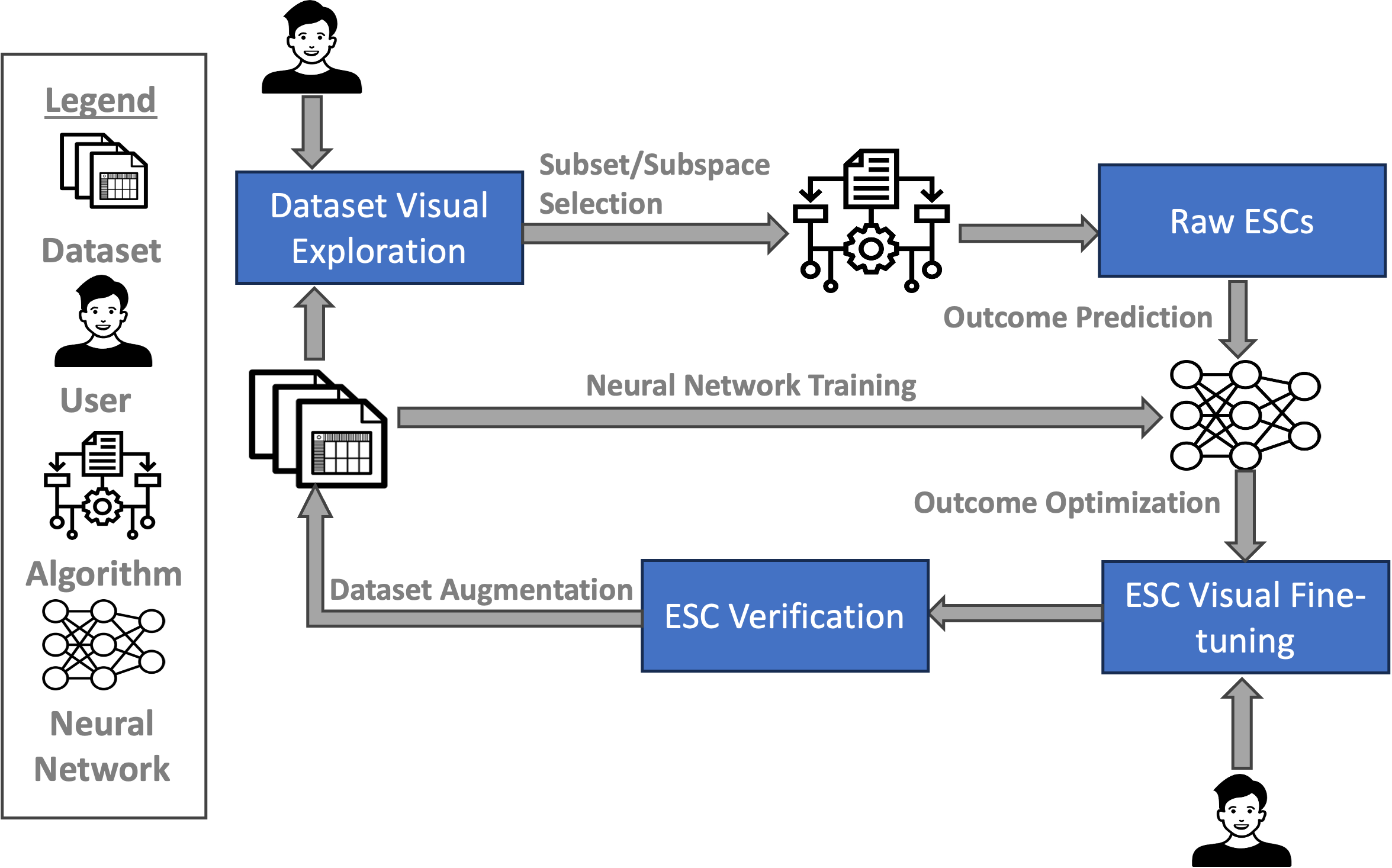
Figure 1: Our three-phase workflow.

III Overview

Fig. 1 presents an overview of our methodology. It comprises three phases centered around training an assistive deep neural network (DNN) that becomes increasingly adept at recommending useful empty space configurations (ESCs) for the target (domain) application’s possibly multiple objectives. The process begins with a fully untrained DNN, where the user (typically a domain expert) and our empty space search algorithm (ESA) collaborate to identify initial ”raw” ESC candidates; this is depicted in the top branch of Fig. 1. These candidates are then interactively refined by the user using visual tools and applied within the target application, as shown in the bottom branch of Fig. 1. The application is run with these configurations, and their performance is measured. Once verified, these ESCs augment the dataset and are used to train the DNN (per the middle branch of Fig. 1). As the DNN improves, the user’s involvement gradually decreases.

Ultimately, the pipeline operates autonomously: the ESA identifies ESC candidates, the DNN optimizes and approximates the target application’s outcomes, and the dataset is continuously updated with new ESCs. In the following we describe the various components of this workflow.

IV Empty Space Search Algorithm

The search for empty regions in a high-D data space is a main premise in our work. The challenge here is to describe this space effectively, without enumerating all of the points that reside within each continuous (empty) region. A key requirement is that interior points within an empty space should be far from known points. To locate the emptiest region within a group of data points, one could use Delaunay Triangulation, where the circumscribed center represents the emptiest point. However, as mentioned, computational-geometry methods face the curse of dimensionality.

We instead propose an agent-based approach. Here, the agent is repelled from known data points if it comes too close and is attracted back if it strays too far. This premise is the aim of a physics-inspired function called the Lennard-Jones Potential, which is the principle guiding our heuristic search algorithm. A particular advantage of this scheme is that it is easily parallelizable. Agents can be deployed throughout the high-D data space and operate autonomously to identify empty space points. Next, we describe this physics-inspired search method in detail.

IV-A Physics Background: The Lennard-Jones Potential

There are multiple causes of intermolecular interactions, including Van der Waals forces, hydrogen bonds, and electrostatic interactions. Some of the forces are repulsive and others are attractive, so that a dynamic equilibrium of molecules is maintained. The Lennard-Jones (L-J) Potential [35] (see Fig. 2 for an example) is a popular model of intermolecular interactions and is described as:

$$V(r)=4\epsilon\left[(\frac{\sigma}{r})^{12}-({\frac{\sigma}{r})^{6}}\right]$$ (1)

where $r$ and $V(r)$ are the distance and potential of a pair of particles, and $\epsilon$ represents the depth of the potential well, correlating to the strength of the interaction between two particles. $\sigma$ represents the effective diameter of the particles, that is, the distance at which the total potential energy between two particles becomes zero. At distances less than $\sigma$, the repulsive force dominates, causing the potential energy to increase sharply. At distances greater than $\sigma$, the attractive force is stronger, pulling the particles together, but this force diminishes with $r$. The nature of intermolecular interactions keeps a point dynamically steady in a local region. Our search algorithm uses the L-J Potential function.

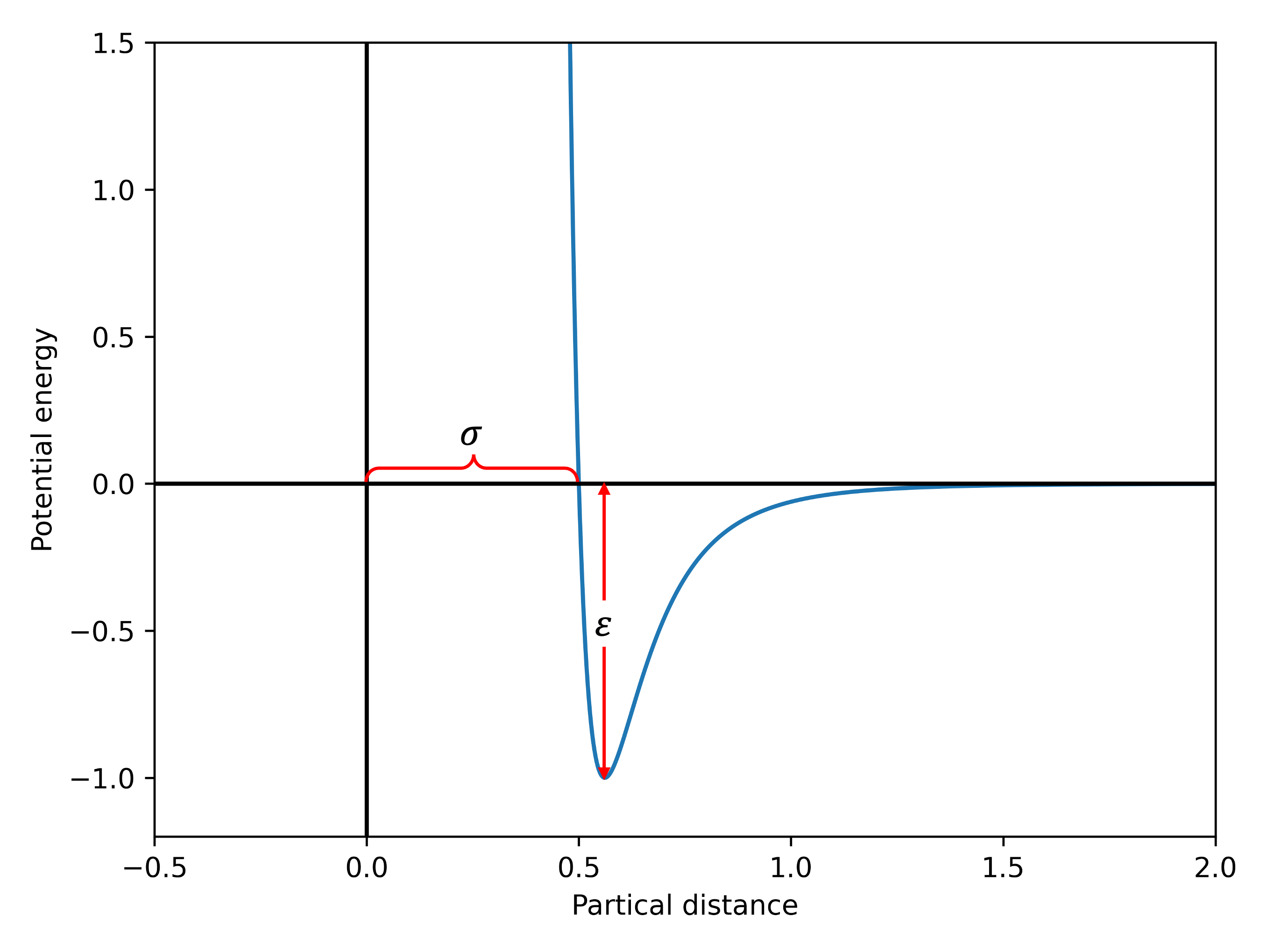
Figure 2: An example of Lennard-Jones Potential. The $x$ axis is the distance between particles ($r$) and the y axis is the outcome $V(r)$. The potential is positive when the particle distance is less than $\sigma$, indicating a repulsive force, and negative for larger distances, where there is an attractive force. The minimum potential (strongest attraction) is $-\epsilon$.

IV-B Our Lennard-Jones Potential Based Search Algorithm

We assume that there is a possibly small initial dataset with verified configurations, and we populate the high-D search space with these known configurations. Then we place an agent in this space to search for Empty Space Configurations (ESC)—the raw ESCs in Fig. 1. The agent starts from a randomly sampled initial position and uses the L-J Potential function to move to a location where the potential becomes zero. This trajectory is sampled along the way to form a set of raw ESCs.

The vector intermolecular force $F(r)$ driving the agent is:

$$F(r)=\frac{dV(r)}{dr}=24\frac{\epsilon}{\sigma}\left[2\left(\frac{\sigma}{r}\right)^{13}-\left(\frac{\sigma}{r}\right)^{7}\right]$$ (2)

To adhere to physical reality, we use the resultant force $\Sigma\vec{F}$ to determine the direction of motion $\vec{d}$, rather than simply using $V(r)$. However, we will stop the agent if $||\Sigma\vec{F}||$ falls below a threshold as this indicates it has moved beyond the data manifold. $\Sigma\vec{F}$ is the sum of forces due to the agent’s $k$ nearest neighbors in the dataset:

$$\Sigma\vec{F} =\sum_{i}^{k}\vec{u_{i}}F(r_{i})\qquad\vec{d} =\frac{\Sigma\vec{F}}{||\Sigma\vec{F}||}$$ (3)

where $k$ is the number of neighbors and $\vec{u_{i}}$ is the unit vector from the agent to the $i$th neighbor.

Set the number of neighbors $k$, the particle effective diameter $\sigma$, the number of search steps $n$, the step size $\alpha$, the discount factor $\gamma$, the vanishing threshold $\delta$ and the rollout interval $j$;

Initialize a trajectory $\tau=[]$ and an agent $\pi=\mathbf{c}$ where $\mathbf{c}$ is a random coordinate; set cumulative magnitude $L=0$, momentum $\vec{m}=\vec{0}$;

Specify constraints on agent:

  $f_{1}(\pi)<=0$; $f_{2}(\pi)<=0$; …, $f_{p}(\pi)<=0$;

for i …$n$ do

    if i % $j$ == 0 then

       Add current coordinate of $\pi$ to $\tau$;

      

    end if

   Get $k$ nearest neighbors of the agent from the dataset;

    Use Eq. 3 to calculate $||\Sigma\vec{F}||$ and $\vec{d}$;

    if $||\Sigma\vec{F}||<\delta$ then

       return $\tau$;

      

    end if

   

   $\vec{d}=(\vec{d}*||\Sigma\vec{F}||+\vec{m}*L)/(L+||\Sigma\vec{F}||)$;

    $\pi=\pi+\vec{d}*\alpha$;

    $L=\gamma*L+||\Sigma\vec{F}||$;

    $\vec{m}=\gamma*\vec{m}+\vec{d}$;

    $\vec{m}=\vec{m}/||\vec{m}||$;

   

   if $\pi$ violates any constraint $f$ then

       return $\tau$;

      

    end if

   

end for

return $\tau$;

Algorithm 1 Empty-Space Search for a Single Agent

Alg. 1 illustrates the details of our empty-space search. It returns the trajectory $\tau$ of an agent, where each element is a raw ESC. Users can set two accuracy levels for the DNN, defined by the DNN’s acceptable prediction error, measured in %. When the DNN performs worse than the lower accuracy level, which occurs in the initial learning phase, it cannot reliably estimate the value of an ESC. In this case we set $\gamma=0$, causing the agent $\pi$ to simply move in the direction of $\vec{d}$; when converged it returns the end of $\tau$ as the ESC. This strategy encourages the algorithm to identify as many gaps as possible, fostering the development of a robust neural network and accelerating training. However, it may also lead to convergence on local minima.

The time complexity of ESA is $O(dknp+np\log N)$ where $d$ is the dimensionality of the dataset, $k$ is the number of nearest neighbors, $n$ is the number of search steps, $p$ is the number of agents, and $N$ is the size of the dataset. $O(dknp)$ represents the time complexity to determine the next step, while $O(np\log N)$ represents the time complexity to query $k$ nearest neighbors; the space complexity of ESA is $O(dp)$. In contrast, the time and space complexity of Delaunay Triangulation is $O(N^{\lceil{d/2}\rceil})$, as mentioned before. ESA is considerably more efficient in both time and space.

Once the DNN has developed further (phase 2 in the workflow of Fig. 1) and meets the lower accuracy level, we begin incorporating a momentum $\vec{m}$ with factor $\gamma>0$ to move the agent along. This mechanism considers historical directions alongside those calculated by Eq. 3, resulting in a smoother update for the direction of $\pi$. We constrain $\gamma<1$ to prevent a long-term effect; thus, the effect of historical forces gets lower and lower with each search step. The momentum mechanism encourages the agent $\pi$ to explore the space in a broader range before converging to the empty region, leading it to discover global minima. Then, upon terminating it returns $\tau$ as a list of ESCs. Eventually the DNN is accurate enough to achieve the higher accuracy level. We then improve $\tau$ by DNN-enabled gradient ascent and pick the best result.

Fig. 3 shows our algorithm’s outcomes for a 2D dataset. Agents tend to converge to a small region without momentum (Fig. 3(a)), but to a larger region with momentum (Fig. 3(b)). Larger regions are explored more thoroughly in the latter case while smaller gaps are left alone.

We note that the ESA works in local space with simple calculations and scales well to higher dimensions and larger datasets (see also Sec. IX). As mentioned, since each agent operates independently, it is feasible to expedite the empty space search using a GPU and deploy a large batch of agents concurrently. DT does not offer this kind of parallelism.

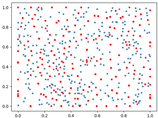
(a)

(b)

Figure 3: Given 300 random samples (blue) and 600 random agents (red) in 2D space, we show the results of ESA (a) without and (b) with momentum.

V GapMiner

Our visual analytics system, GapMiner, combines data space exploration and HITL to aid users in identifying promising ESCs during the first two phases of the workflow when the DNN is not yet fully trained.

V-A Design Goals

Following the design model devised by Munzner[46], we studied popular datasets on Kaggle, reviewed recent research in our example domain (computer systems [60]), and interviewed several domain experts. This study yielded the essential features an effective visual analytics system for empty-space search should have:

• F1: Subset/Subspace selection. Users often focus on specific data segments; e.g., a system designer with a limited budget might want to explore moderate options first. Sometimes these subsets are so small that their key features are hidden within the entire dataset. Hence, explorations within data subspaces must be supported.

• F2: Data distribution visualization and cluster highlighting. For data with categorical outcomes, each label typically forms a distinct cluster. For continuous outcomes, high and low values usually don’t overlap. Highlighting clusters and visualizing distributions will help users identify valuable empty spaces for exploration.

• F3: HITL ESC fine-tuning. While the ESA identifies numerous ESCs, they are not fully refined configurations, but only starting points for exploration. Users should be able to define empty space search regions and refine raw ESCs based on their expertise.

• F4: ESC neighbor visualization. In order to select promising ESCs, users need to understand the distribution of their neighbors, i.e., the shape of the empty space (hypersphere, paraboloid, hyperbolas, etc.), to aid informed decision making.

• F5: Outcome evaluation. Users must be able to evaluate the performance of an ESC which sometimes is gauged by more than a single outcome variable. Additionally, the cost of obtaining certain configurations can also be important.

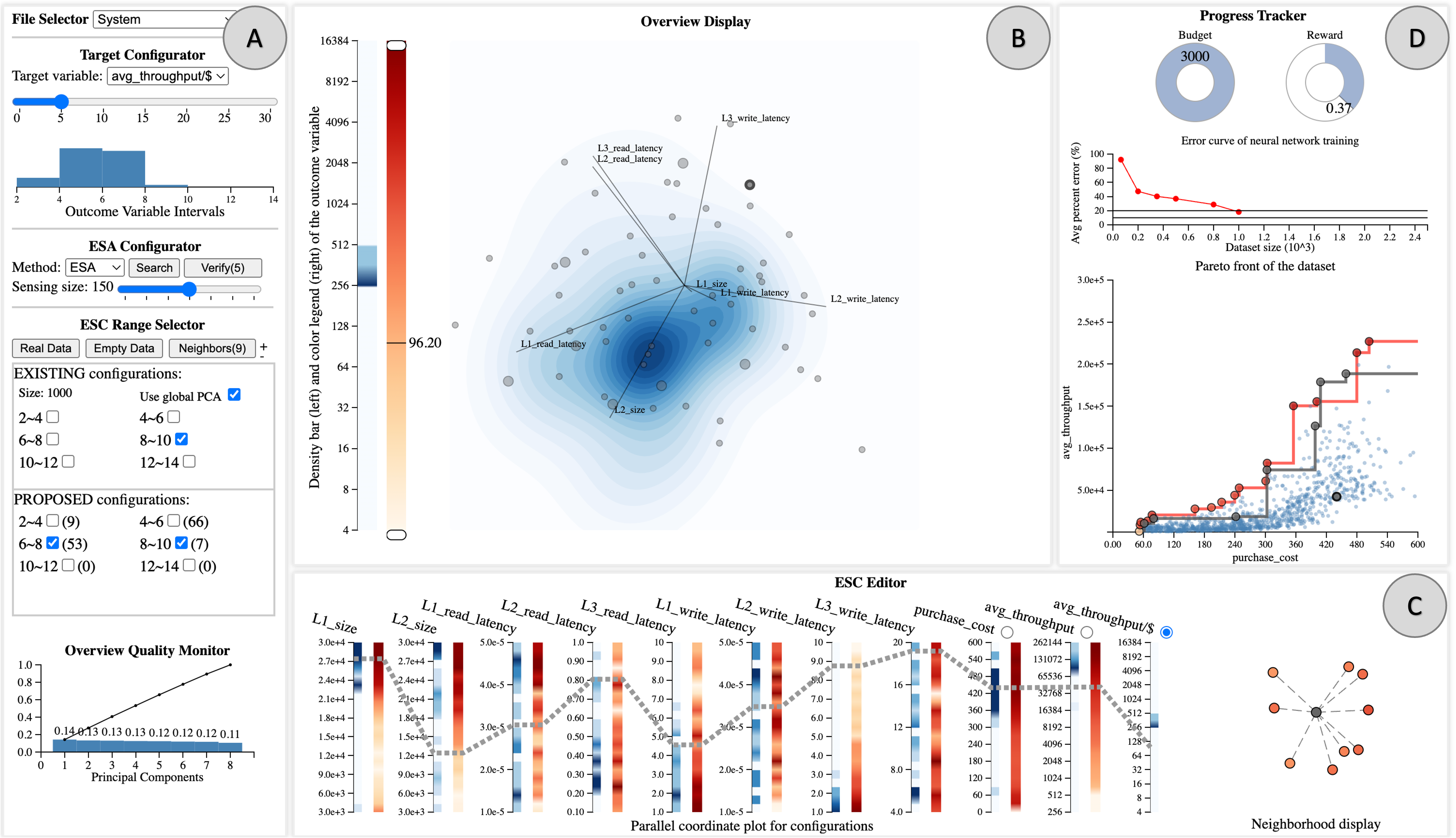
Figure 4: GapMiner visual interface where a selected ESC is reflected in all displays. (A) Control Panel. From top to bottom: (a) File Selector to load a dataset of initial verified configurations with values for all parameter variables. (b) Target Variable Configurator with an interface for breaking its value range into discrete intervals. (c) Empty Space Algorithm (ESA) Configurator to select the ESA and a slider to set the ESC batch size. (d) Empty Space Configuration (ESC) Range Selector to control which target variable intervals are used for display and ESC proposals. (e) Overview Quality Monitor screeplot that shows the amount of data variance captured by the Overview (PCA) Display. (B) Overview (PCA) Display with data distribution contours, raw or modified ESCs rendered as points, and color legends. (C) Empty Space Configuration (ESC) Editor. From left to right: (a) Parallel Coordinate Plot where users can configure ESCs starting from a raw ESC or an existing configuration. (b) Neighbor plot of the selected ESC providing a local view of the distribution of its nearest existing configurations. (D) Progress Tracker. From top to bottom: (a) Budget/Reward Display that captures the aggregated evaluation cost and merit of the ESC exploration so far. (b) Training Status Display of the assistive DNN. (c) Pareto Frontier Plot that shows the Pareto frontiers of existing configurations (red) and ESCs (gray) with respect to two user-chosen merit (target) variables.

V-B Terms, Color Semantics, and Representations

Fig. 4 shows the GapMiner interface. The dataset displayed consists of a set of multi-tier cache configurations used to replay a real-world block I/O trace, each with three devices: $L1$, $L2$, and $L3$. Each cache device has three variables: $size$ and average read/write latencies (the size of the backend storage device $L3$ is fixed for all configurations and so it is not included). See Sec. VII for more detail. The target variables are average throughput and total purchase cost, used to evaluate the performance and cost of each configuration, respectively.

The term existing configurations used in Fig. 4 (A) refers to configurations in the dataset that have been verified, whereas proposed configurations are configurations proposed by the various available ESC search algorithms but which have not been verified yet. GapMiner distinguishes these two types with different colors. All gray points and lines in the interface represent proposed configurations, while everything related to existing configurations is colored blue, including density contours in Fig. 4 (B), histogram bars in Fig. 4 (A) and Fig. 4 (C), and scatter points in Fig. 4 (B). Additionally, we apply an orange-to-red colormap in Fig. 4 (D) to encode target variables in the Pareto front of existing configurations, and the same colormap in Fig. 4 (C) to encode target variables of existing neighbors around the proposed one.

Zhang et al. [64] illustrated the benefits of contour maps in exemplar identification while Li et al. [36] combined density contours and scattered points for outlier examination. In the PCA map in Fig. 4 (B), we follow their design pattern, employing density contours to abstract existing configurations and scattered points to denote proposed configurations. In the PCP, we visualize proposed configurations as dashed lines and existing configurations as solid lines shown in Fig. 4 (C).

Next we describe all of GapMiner’s components in detail, referring to the Interface in Fig. 4 and the Design Goals they satisfy.

V-C Control Panel

After loading the dataset containing the initial verified configurations with values for all variables, the user will head to the Target Configurator (A) to select a target variable subject to optimization. The target variable can either be a native outcome variable such as performance or cost, or it can be a ratio like performance/cost. The latter provides quick insights into efficiency, while the former two can be optimized within our multi-objective optimization to account for the user’s preferences. The user can now utilize the slider below to evenly split the range (F1) of the selected target variable. This action divides the dataset according to the selected value interval and the histogram below visualizes the distribution (F2). The user can now choose among one of three empty space search methods from the dropdown menu: the physics-based ESA described above, random sampling, Pareto improvement, and a baseline (see Sec. VI).

The ESC Range Selector enables users to select one or more subsets of the data, as specified in the Target Configurator (see above), using the checkboxes in the “existing”/“proposed” group (F1). The “Size” in the verified “existing” group indicates the number of these configurations.

V-D Overview Display

The PCA-based Overview Display (B) linearly transforms the high-dimensional data space into a variance-maximizing 2D projection. It is an intuitive way to visualize data distributions and identify clusters (F2), We chose the linear dimension reduction provided by PCA since evaluating results from nonlinear methods like tSNE is challenging and connecting their embedding space to the original space is difficult.

Once a checkbox is selected in the ESC Range Selector, the associated subset of the data will be displayed in the Overview Display either as density contours (“existing”) or as scattered points (“proposed” or selected via other means). The scented color legend bars on the left map values to color: the left one represents the target variable density of the chosen subset, while the right one shows the value range of the entire dataset. The “Use global PCA” checkbox in the ESC Range Selector (A) determines whether the PCA layout is applied to the chosen data subset (F2) or the entire dataset; the PCA map will update accordingly. Applying the PCA layout to the currently selected data subset will reduce the layout loss and make the display more accurate and focused. This improvement is quantified in the Overview Monitor scree plot.

The loading vectors in the PCA display represent the projection of Cartesian axes from the original space, forming a biplot. Due to the linear nature of PCA, any value change along one axis in the original high-D space results in a proportional update along the corresponding loading vector in the PCA map. Additionally, the loading vector projection is translation-invariant; any point can be chosen as an anchor to project the Cartesian basis. We derive this mechanism in closed form in App. A.

V-E Empty Space Configuration (ESC) Editor

This interface panel has two displays: a PCP (left) where an ESC can be configured and refined and a neighborhood plot (right) that shows the topology of the ESC’s immediate point neighborhood.

PCP display. The PCP allows users to fine-tune a proposed ESC or propose one on their own. It is the most effective display for this task as it provides simultaneous access to all variables and allows for easy adjustments through simple mouse interactions. For additional insight we provide two scented bars along each PCP axis (F1, F2).

The (blue) density bar next to each axis shows that variable’s value distribution in the currently chosen data subset, with darker blue indicating higher density in that range. This visual information complements the density contours in the Overview Display (B). The correlation bar next to the density bar shows the relationship between the variable and the selected target variable, calculated from all existing configurations. Users can select the target variable for this calculation by clicking the radio button along its corresponding axis (for example in (C) there are three such variables—two native variables and one ratio variable). For a linear relationship, the orange-red bar along each variable axis indicates whether the correlation with the selected target is positive or negative. For a nonlinear relationship, it reveals which value interval corresponds to a higher target value (darker color) and which to a lower target value (lighter orange).

Lastly, when users modify an ESC in the PCP, its 2D position in the Overview Display is updated proportionally along the direction of the corresponding loading vector. This is particularly useful when there is an empty space in the Overview Display, providing users with important feedback that they are on the right track.

Neighborhood Plot. This display, located to the right of the PCP, helps users understand the shape of an empty space as well as the neighbor distribution of the associated ESC (F4). To create this visualization we devised a dedicated dimension-reduction method we call cos-MDS to visualize the neighbor distribution around an agent. This method embeds the agent at the center and places its immediate high-D neighbors around it. The distance from each neighbor to the agent in the visualization represents their true distance in the high-D space. Neighbors’ pairwise cosine distance, measured from the agent, approximates their true cosine distance in the high-D space. The method effectively reveals the distances and distribution of neighbors around the agent, as well as the shape and topology of the empty space (fully enclosed, semi-enclosed, cluster boundaries, or anti-hub outliers).

cos-MDS is inspired by MDS to arrange the neighbors around the agent such that the shape and topology of their constellation is revealed in 2D. Similar to MDS, we normalize each agent-neighbor vector to the unit hypersphere, compute a pairwise cosine-distance matrix, perform eigenvalue decomposition, and use the top two eigenvalues and their eigenvectors for the low-dimensional embedding. Finally, we scale the low-D agent-neighbor vector to the true length in the original space (see App. B for a detailed description.)

The example shown in the ESC Editor (D) has neighbors uniformly surrounding the configuration, and the distances to it are almost equal. In essence this is a case where the empty space is fully enclosed—a pocket in a high-D point cloud. Users can also change the number of neighbors by clicking the +/- button next to the Neighbors button in the control panel. This provides a more comprehensive perspective to understand the empty space, e.g., in a hypersphere, within a paraboloid, or between hyperbolas. Detailed examples can be found in App. B.

V-F Progress Tracker

The Progress Tracker (D) keeps the user abreast of the achievements made so far (F5). It has three main components (top to bottom): (1) a Budget/Reward Display that captures the aggregated evaluation cost and merit of the ESC exploration so far, (2) a Training Status Display of the assistive DNN, and (3) a Pareto Frontier Plot that shows the Pareto frontiers of existing configurations (red) and ESCs (gray) with respect to two user-chosen merit (target) variables. We now present these three displays in reverse order according to their use in practice.

Pareto Frontier Plot. The Pareto frontier is an effective mechanism for evaluating a set of proposed configurations in the presence of multiple target variables. To reduce visual complexity we currently restrict the number of target variables to two. Our goal is to aid users in recognizing trade-offs among the two target variables and identify ESCs that can expand the frontier (push the envelope) at desirable trade-off points on the curve.

We use the following color scheme in this plot: (1) existing configurations are colored blue, with their Pareto front connected by edges. The configurations defining these edges (and the edges themselves) are colored by their respective target variable values according to the red-toned color map to the left of the Overview Display and are represented as larger nodes there; (2) proposed configurations are colored gray, with their Pareto front connected by gray lines. Comparing the two curves facilitates an understanding of a candidate ESC’s merits in the context what is known already and what the user’s trade-off preferences are.

When the user modifies an ESC (say, in the PCP) its position in the grey Pareto plot and frontier (and Overview Display) will update accordingly. Then, upon verification, the ESC is added to the “existing” set, its Pareto point is colored blue, and the red Pareto front updates.

DNN Training Status Display. As mentioned, once the user loads the initial dataset, GapMiner trains an assistive DNN on the backend for ESC performance prediction. The DNN evaluates the performance of each proposed configuration before verification takes place. The testing error of the DNN is then shown in the DNN Training Status Display. We observe in (D) that there is a fairly large error in the initial stage (first part of the curve), hence at that stage user involvement is typically necessary to identify optimal configurations. The DNN is retrained whenever new configurations are added to the dataset and are verified.

The two horizontal lines in the display signify the user-specified DNN error tolerance. The DNN can be used to filter out poor configurations once it reaches below the first line, and it can be used for configuration optimization once it reaches below the second line. Details of the progressive search pipeline are introduced in Sec. VI.

Budget/Reward Display. There are also two other important objectives in practical applications, namely cost and benefit/reward. Maintaining a balanced optimization across both of these objectives is challenging but crucial. To gauge the progress of reward quantitatively, we incorporate the concept of Pareto dominance area [10] into the Progress Tracker (D) to monitor the Pareto front of the dataset. The Pareto dominance area is a well-established quality metric in multi-objective optimization that measures the volume of the objective space dominated by the Pareto front. As more ESCs are identified and verified, the Pareto front should extend further, dominating a larger area in the plot.

On the other hand, configuration verification can be expensive or time-consuming. For example, in the dataset we demonstrate, users had to purchase a configuration and run it for a week to obtain the real average throughput. In our application, thanks to CloudPhysics [60], we could simulate a configuration quickly to get an approximated result. However, verification costs are unavoidable in many scenarios. To address this, we provide a budget counter in the Progress Tracker (D) to remind users of the aggregate cost of continued ESC verification.

We chose donut charts for both the Pareto Dominance-based Reward Display and the Budget Display due to their compactness and their ability to effectively convey proportional data at a glance.

VI DNN-Assisted Configuration Search Pipeline

While GapMiner effectively assists users in the search for optimal ESCs, manually identifying a large number of optimal ESCs can be tedious. To address this challenge, we propose a pipeline that trains an assistive DNN to eventually automate this process, positioning the analyst as a mentor to the DNN. This section provides a breakdown of the pipeline, as illustrated in Fig. 1. We begin by describing the various search methods we have implemented and then describe their role in the DNN-training process.

VI-A Configuration Search Methods

In addition to the physics-inspired ESA, GapMiner integrates three more methods for investigating the empty space: random sampling, Pareto improvement, and a blank baseline. The blank baseline is a configuration with every variable set to 0.5, locating it at $[0,0]$ in the PCA map. This strategy provides no hint from the initial position, requiring users to rely solely on GapMiner interactions to optimize a configuration.

Random sampling, as the name suggests, samples configurations in a random manner. Pareto improvement, on the other hand, starts from the Pareto front of the existing set, allowing users to improve a configuration from a Pareto-optimal point. While Pareto improvement can be a good starting point for breakthroughs, it does not provide insights into the empty space. Empty-space search and random sampling are likely to find configurations better than those based on the Pareto front. Initially, we used another strategy, random walk, but experiments showed it was statistically similar to random sampling, so we did not include it in GapMiner.

All of these methods, including ESA, work as initial configuration hints for users in the startup stage. Users can then fine-tune the configurations proposed by these strategies to get better configurations. Additionally, users can also let the algorithm propose and verify a batch of configurations. The batch size is determined by the slider in the ESA Configurator in Fig. 4(A). Once new configurations have been verified, they will be added to the “existing” configuration set and used to retrain the DNN.

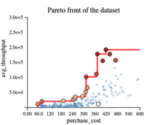
(a)

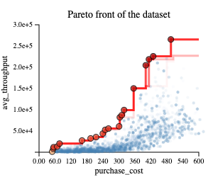
(b)

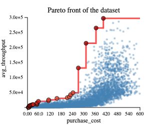
(c)

Figure 5: An example Pareto front at the three key stages. (a) The initial stage when the DNN has just started training. There are only few configurations in the “existing” set, colored blue. (b) The front when the DNN has achieved $t_{1}$. The “existing” set has grown. (c) The front when the DNN has achieved $t_{2}$. The “existing” set now covers much of the front’s interior.

VI-B Pipeline Throughout the DNN Training

Fig. 5 shows the Pareto front development at the three pipeline stages. We now describe these in more detail.

Initial Stage. In the early stage the dataset is still small and its empty space regions remain largely unexplored. With the data set still being insufficient to train a usable neural network, users can utilize GapMiner and its various exploration tools to identify empty spaces, propose new configurations, optimize them, and verify their effectiveness. In our studies with analysts we found that combining various configuration search strategies yields more diverse and higher-quality results to grow the dataset than sticking with only one search algorithm. Additionally, the visual feedback provided by the Progress Tracker incorporates elements of gamification. It not only indicates progress but also challenges users to find high-quality ESCs in a cost-effective manner.

Developed Stages. As the set of existing configurations grows, paying attention to the error plot in Fig. 4 (D) becomes crucial. As mentioned, it shows the average percentage error of the DNN along with the two user-set accuracy levels $t_{1}$ and $t_{2}$. Once the error is below $t_{1}$, the system will use the DNN to evaluate the proposed configurations, improving the quality of suggestions. Users can rely more on the system at this stage but still apply their domain knowledge to enhance results. Then, when the error drops below $t_{2}$, the system will go one step beyond, using gradient ascent of the DNN to refine configurations further. The performance estimation now becomes accurate enough to find optimal configurations without user supervision. At this stage, the DNN and ESA can completely replace the user.

VII Application Example

(a)

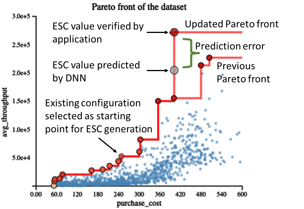
(b)

Figure 6: Improvement of the Pareto front by interaction in the PCP followed by DNN estimation of the target values and subsequent verification in the domain application which revealed a lack of DNN training. (a) PCP showing the result of some user interactions; (b) annotated Pareto front.

To illustrate our pipeline, we present a use case in the application area of computer system optimization (see Sec. V-B for an introduction to the data). Fig. 4 shows a snapshot taken of the interface during this session.

We used a trace of a real workload run on actual machines, provided by CloudPhysics [60]. We chose trace w11, which captures a week of virtual disk activity from a production VMware environment. This trace file contains I/O requests recorded over the week, which can then be replayed using either a physical machine or a simulator of that machine. To save time and energy, we used the simulator for all our experiments.

Given the size of the workload, evaluating a configuration is an expensive process. Additionally, there is a vast number of potential multi-tier configurations. Thus, conducting an exhaustive search of this space is infeasible, making the efficient identification of optimal configurations highly valuable to system administrators [22, 21].

To begin, we collected a small number of configurations with the help of system experts. We then invited a field expert to try GapMiner, ESA, and the overall pipeline. Empirically, a configuration with good avg_throughput is usually more expensive; thus the expert’s goal was to find optimal configurations with good performance at a lower price.

The expert began by loading the dataset and setting the two DNN thresholds: $t_{1}=20\%$, $t_{2}=10\%$. Next, he selected $\mathit{avg\_throughput}/\$$ as the target variable since it captures a reasonable first compromise between the two main objectives $\mathit{avg\_throughput}$ and $\mathit{purchase\_cost}$. After bracketing the target variable he learned from the range histogram (Fig. 4 (A)) that there were just a few configurations in the best and worst value intervals. Next the expert ran the ESA algorithm and then checked the (higher) 8~10 interval of the “existing” group and the 6~8 and 8~10 groups from the “proposed” configurations found by the ESA (see (Fig. 4 (A)). This action revealed the former as a density plot and the latter as scattered points in the Overview Display (Fig. 4 (B)). A Pareto front, computed from the “proposed” configurations, appeared in the Pareto front display (Fig. 4 (D)) in grey, with the points defining the front being drawn as larger nodes in the Overview Display.

The red curve in this Pareto front display shows the front of the “existing”, verified configurations, and the configurations that define it are colored by the selected target variable, $\mathit{avg\_throughput}/\$$, according to the red-toned colormap to the left of the Overview Display. The expert noticed that the grey front only surpassed the red front in the high $\mathit{purchase\_cost}$ area but had poor $\mathit{avg\_throughput}$ for low $\mathit{purchase\_cost}$ configurations. He decided not to evaluate or verify any of the proposed ESCs but rather focused on the red Pareto front in the low $\mathit{purchase\_cost}$ area. He found a lower-performing configuration there, indicated by its orange, less vibrant red color (see Fig. 6(b)). He first tried to improve it by moving it to the dense region in the Overview Display where the high-performing “existing” configurations reside, but this strategy failed. To investigate why, he examined the scree plot in Fig. 4 (A) and noticed the slow growth of the aggregate curve. This essentially means that the PCA map did not explain much of the data variance and so moving configurations along loading vectors that pointed directly to the dense region was not sufficient. Some short or nearly orthogonal loading vectors like $\mathit{L1\_size}$ or $\mathit{L1\_write\_latency}$ might also matter.

Looking for an alternative approach he turned to the density bars in the PCP to learn about the per-variable distributions. Fig. 6(a) shows the PCP with the polyline of the Pareto configuration under consideration colored in orange, indicating its lower performance. And indeed, despite residing in a dense PCA region, this configuration suffered from sub-optimal $\mathit{L1\_size}$ and $\mathit{L1\_write\_latency}$ settings (it falls in less dense and lightly colored regions in the density and correlation bars, respectively, for both variables). These variables minimally contributed to the PCA space but apparently significantly impacted the target variable outcomes.

The expert adjusted the configuration to dense intervals in both variables, as indicated by arrows in Fig. 6(a). He then asked the DNN to estimate the value for $\mathit{avg\_throughput}$ and calculated other target variables, which showed significant improvement and expanded the Pareto front in the upper region (grey node in Fig. 6(b). Pleased, the expert clicked the Verify button to obtain the true performance. After some time, the verification results showed that this configuration was even better than the DNN prediction (red node at the top of Fig. 6(b)), and the dominance area increased significantly.

While this was a positive development, the expert also realized that the DNN did not perform well in the upper region of the Pareto front (see the large prediction error in Fig. 6(b)). More configurations in that range were needed to train the DNN effectively. To address this, the PCP interface enables users to select specific value intervals and run ESA exclusively within these intervals to generate ESC batches.

As the expert created more ESC batches and verified some of the generated ESCs, the DNN eventually reached the $t_{1}$ threshold. At this point, the expert was able to rely more on the DNN to assess the quality of ESCs and he started to only focus on the ESCs located on the proposed Pareto front for verification. Finally, once the DNN surpassed $t_{2}$, the AI model completely took over the expert’s role. As shown in Fig. 5, this three-stage pipeline increased the dominance area from 0.27 to an impressive 0.56, more than doubling it.

VIII User Study

We conducted a user study to evaluate GapMiner with the same system dataset (see App. D for a detailed description of this experiment). We asked 10 graduate students with CS backgrounds to perform an optimal-configuration search from an initial stage that had 200 configurations in the set. The users could make full use of GapMiner with all search methods: ESA, random sampling, Pareto improvement, and the blank baseline. The batch size for searching was fixed to 50 for all users. They could click the search button multiple times, but they could click the verify button only 5 times to get the true $\mathit{avg\_throughput}$. Once they believed they had a good configuration, they ran one of their alloted verifications. We calculated the dominance area and updated it in the reward donut chart in Fig. 4 (D)[10] as the evaluation metric.

VIII-A Result Analysis

We compared the GapMiner-aided performance of the users with the outcomes achieved with (1) ESA-based search only and (2) verifying the initial random samples directly, in order to see whether GapMiner helped users with the task. Noticing that users clicked search three times on average, we set the batch size to 150 for the two baselines (ESA and random) to match the user behavior, calculated the Pareto front estimated by the naïve neural network, and then verified the naïve Pareto front. We ran each baseline 10 times to match the number of participants. We did not choose the top five for verification in the baselines because we found no difference between verifying the top five and the whole Pareto front in the dominance area. Our results are given in Fig. 7. We can see a clear advantage in user performance compared to the two baselines. The average reward of ESA is 0.319 and the average reward of random sampling is 0.295, both of which are much lower than our users’ average reward, 0.393. 7 users reached higher rewards than ESA and 9 reached higher rewards than random sampling.

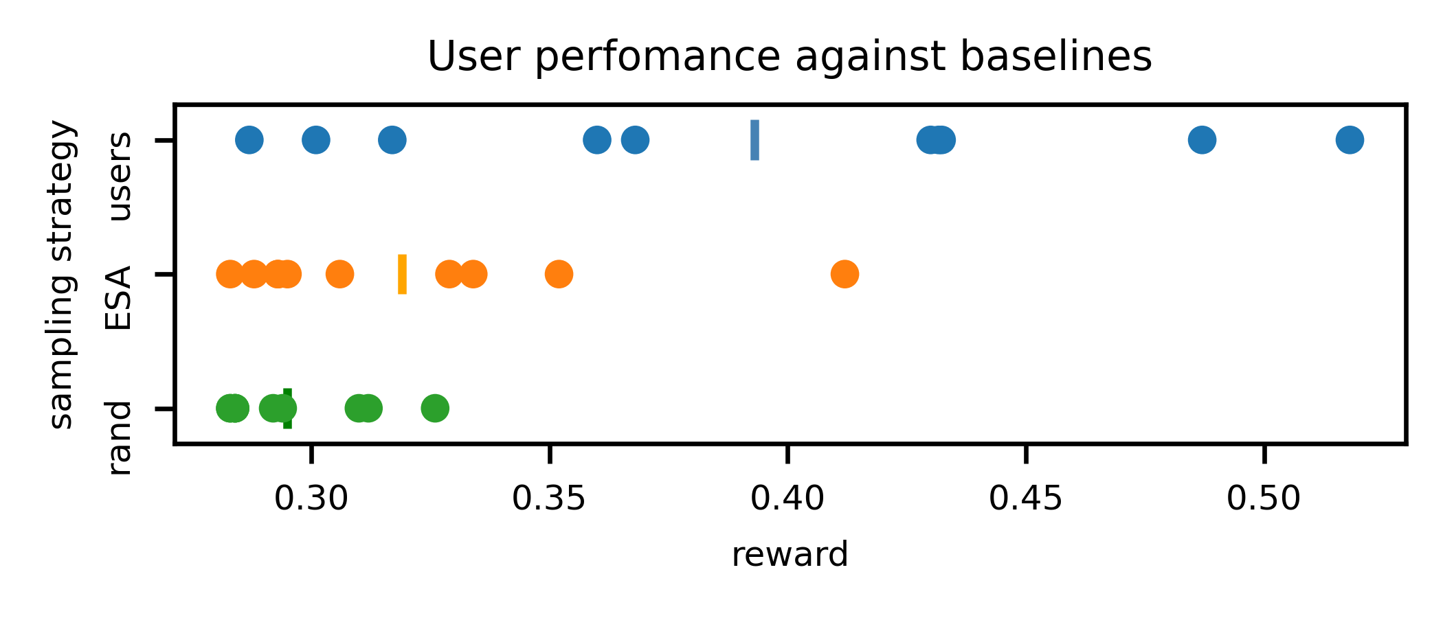
Figure 7: Rewards achieved by users, ESA, and random sampling. Each dot represents a search round (5 verifications). The reward is defined by dominance area in the Pareto plot. The bar within each strip is the mean value.

We also did a between-subjects ANOVA with Tukey’s Honestly Significant Difference (HSD) to analyze our data’s statistical significance; the analysis is shown in Tab. III in App. D. Cohen’s $f$ from ANOVA was 0.85, indicating a large effect size. We observe that GapMiner is significantly better than both baselines, while the outcomes between the two baselines do not differ statistically.

VIII-B System Usability

We evaluated the usability of GapMiner with the popular questionnaire System Usability Scale (SUS)[8], which has 10 carefully designed questions that evaluate the system in various aspects. We distributed the SUS to the users after completion of the study and received 5 responses. Our score calculated from the questionnaire was 73. According to SUS score analyses from Bangor et al. [4] and Sauro et al. [53], our system is ranked B (SUS score $>$ 72.6) and is thus considered good (SUS score $>$ 71.1). Therefore, we believe that GapMiner has shown good usability in these initial tests.

VIII-C Comparison Experiments

In addition to testing user performance against algorithms in the initial stage of the pipeline, we also did two experiments to compare how ESA outperforms random methods in developed stages with the help of a neural network. These experiments did not involve users, but employed the well-trained DNN to evaluate and fine-tune ESCs. In the standard pipeline described in Sec. VI, there is an evolutionary DNN working as a critic to determine promising ESCs, and a black box to collect true values. Based on the advice of field experts, we simplified the pipeline in the block-trace scenario by replacing the critic and the black box with a well-trained DNN. The DNN had an average percentage error of $7.9\%$, working as a surrogate model to simultaneously determine good ESCs and verify outcome values.

We employed two baselines in this section: random sampling (RS) and random walk (RW). Random sampling simply samples configurations in the data space. Random walk further walks in a random direction for each of 400 steps, which is the same number we used in the ESA.

In the first experiment, we fast-forwarded to a developed stage that had 1,000 configurations in the dataset instead of iterating from an initial stage. In RS, we randomly sampled 1,500 configurations at once. Starting from the same initial positions as used in RS, we ran ESA and RW, and chose the best ones evaluated by the DNN on each trajectory independently. We repeated the process 50 times to reduce result variance. As before, we used the dominance area as the evaluation metric. The average rewards of ESA, RS, and RW were 0.450, 0.409, and 0.413, respectively. ESA was statistically better than RS and RW, and there was no significant difference between RS and RW. The effect size $\eta^{2}$ was 0.3, indicating that the magnitude of the difference between the averages was large. The full statistical analysis is shown in Tab. V in App. D.

In the second experiment, we fast-forwarded to a stage with 3,000 configurations, using the same surrogate DNN as before. We did the same experiments as in the previous one, the difference being that we used gradient ascent to optimize the best configuration for each trajectory in ESA, RS, and RW. The average rewards were 0.453, 0.418, and 0.422 respectively. There was a statistically significant difference between ESA and random baselines, but no difference between RS and RW. $\eta^{2}$ was 0.3, indicating a large level of effect size. The full statistical analysis is given in Tab. VI in App. D.

All of these experiments and statistical analyses clearly show that our empty search algorithm is much better than random methods.

IX Further Case Studies

In addition to the experiments in system research, we applied our work to an entirely different domain, wine investigation. Furthermore, to show that empty-space search is also a valuable technique for other fields of research, we also demonstrate its potential with adversarial learning in computer vision and Reinforcement Learning (RL) in the MuJoCo environment. Our case studies show the effectiveness of our ESA in a wide range of applications.

IX-A Application in Wine Investigation

We tested our work on the wine dataset [52] to show generalizability to domain-agnostic scenarios. Different from system verification, the wine dataset was collected from the real world. It has 11 chemical properties and a quality rating associated with each wine instance. The 11 chemical properties include {fixed, volatile, citric} acidity, residual sugar, chlorides, {free, fixed} sulfur dioxide, density, pH, sulphates, and alcohol. The wine quality ranges from 3 to 8.

Imagine there is a winemaker fermenting new wine. With quality being the primary concern in mind, the winemaker also wants to minimize the free sulfur dioxide due to potential health issues. We can help the winemaker with GapMiner. First, the scree plot in GapMiner reveals that the PCA space explains about 60% of the variance, which means that the corresponding region in the original space is less variant given a dense region in the PCA space. Next, the distribution of wine quality—3, 4, 7, and 8 in the PCA space (see Fig. 8(a))—illustrates that alcohol and citric acid point to the high-quality region while volatile acidity and density point to the low. Thus, given a wine instance, increasing alcohol and citric acid while reducing volatile acidity and density is more likely to improve the quality. Moreover, the PCP scented widgets indicate that wine quality is independent from free sulfur dioxide. Thus, wine instances in every quality can be fine-tuned to reduce free sulfur dioxide, fitting a wide range of customers.

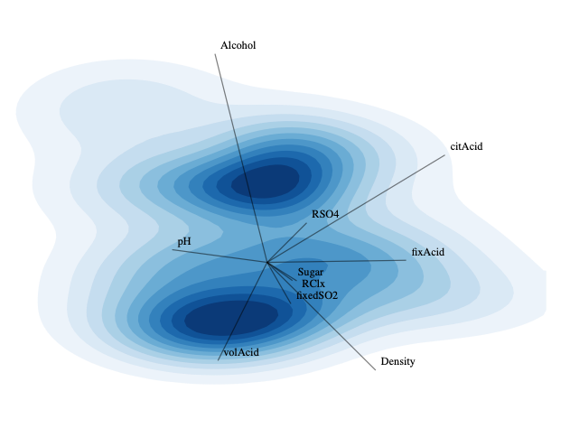
(a)

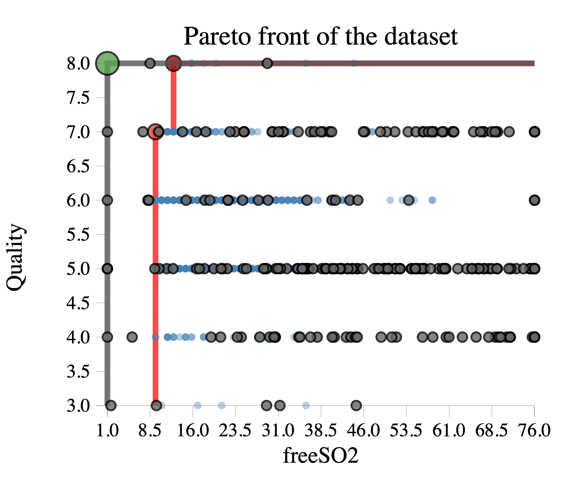
(b)

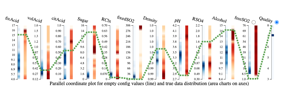
(c)

Figure 8: The key results of GapMiner on the wine dataset: (a)The PCA map showing the distribution of wine instances. The dark region on top represents wine instances with qualities 7 and 8, while the dark region below it corresponds to qualities 3 and 4; (b)ESA results in the Pareto plot. We plot the wine set as blue points and the associated Pareto front as a red line, while ESCs are gray points and the associated Pareto front is a gray line; (c) The full property values of the global optimal wine instance (highlighted in green in (b)).

Looking at the histogram of outcome variable intervals, we noticed that the dataset is severely imbalanced: almost 85% of the wine instances are ranked quality 5 or 6; only 1% are ranked quality 3 or 8, which results in a low prediction accuracy. Therefore, we had to augment the imbalanced quality groups. To do so, we first referred to the PCP scented widgets to learn the property distributions of each quality. For example, wine in quality 4 has higher volatile acidity but lower citric acidity, while that in quality 7 is the opposite. After finding the distributions, we constrained the search range to a dense interval of each property by brushing on the scented widgets in the PCP. Thus, ESA ran in a specific quality region.

Due to the difficulty of obtaining the quality of new wine instances by ourselves, we made it the same as the nearest existing neighbor. This simple but effective strategy is widely used in imbalanced learning [11]. Having identified over 6,000 ESCs, the DNN accuracy improved from 60% to 80% on quality prediction. On the other hand, free sulfur dioxide was integrated with other properties during the empty-space search. Therefore, its value was determined by ESA, which also reduced the DNN’s mean-squared error from 0.018 to 0.002. During the pipeline execution, we were able to find numerous wines with low free sulfur dioxide in each quality. We show the results in Fig. 8 and App. F-B.

To summarize, our ESA, GapMiner, and the pipeline were able to balance the dataset by augmentation, and improve DNN performance. Though we were unable to verify these results in the field, our work could identify numerous innovative wine instances predicted to have good quality or low free sulfur dioxide.

IX-B Empty-Space Images in Adversarial Learning

Latent space has long been studied and has proven to be informative in image generation [31, 1, 37]. In this section, we study the application of GapMiner in the latent space of the MNIST dataset. We spanned the latent space by using an AutoEncoder that transforms a 28*28 image to a 4D point. Additionally, we trained a convolutional neural network (CNN) to do a digit-recognition task and obtained an accuracy of $99.17\%$.

In this experiment, we initialized agents randomly in the latent space and ran ESA without momentum. Then we reconstructed images from empty-space points. The results showed numerous meaningful empty-space images that were falsely classified by the CNN. We show some of the adversarial images in Fig. 9 and describe additional details in App. F-C. It is interesting to note that though these empty-space images in Fig. 9(b) were falsely predicted by the CNN, some of them were mapped to the right cluster by tSNE. While latent space has long been studied for image generation, our work shows that there are many potential adversarial attacks within it, which is an open research area.

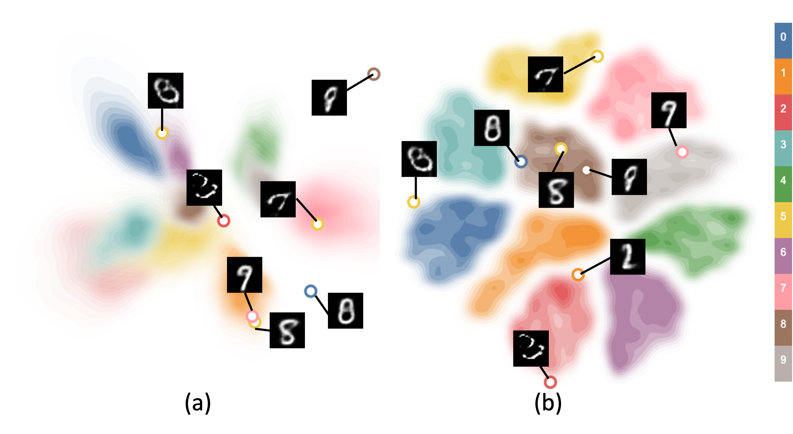
Figure 9: Empty-space adversarial images from MNIST identified by ESA. We visualize the latent space by dimension reduction and highlight some of the adversarial points (compare a point’s color with the colors of the clusters via the color legend on the right). We show the PCA map at (a), which is directly from GapMiner, and the tSNE map at (b). All the images from MNIST are abstracted to contours. We can see clear clusters of digits.

IX-C Empty-Space Search in RL

RL research and its potential to exceed human performance have attracted great attention. Specifically, Actor-Critic [33] is an important RL algorithm that has been widely used as the backbone in a broad range of fields, e.g., in offline meta-RL, network management, and trading [38, 13, 19]. The Actor-Critic algorithm trains a value network to evaluate the value of an observation, and an independent policy network to take an action in reaction to the observation via the feedback from the value network. Here we employed a popular variation, Soft Actor Critic (SAC) [25], for empty-space study.

Mujoco[57] is a physical simulation engine widely accepted for its robot control environments as RL benchmarks. We deployed one of the environments, AntDir, whose task is to control an ant robot to move in a given direction. The reward of AntDir is defined as the velocity towards the right direction, the higher the better. Observations are in a 27D continuous space and actions form an 8D continuous space.

In this case, we studied the possibility of getting a better policy from empty-parameter-space exploration. We trained a SAC agent on the AntDir environment for 200 iterations with a checkpoint saved at each iteration. Next, we extracted all the parameters from the policy network in each checkpoint and converted them to a 22,160D point. There are a total of 200 points in the 22,160D parameter space.

Empty-Space Policies. We first visualized the parameter space using PCA and found a clear training trajectory from a scratch policy to a well-trained one. (The PCA results can be found in App. F-D.) Therefore, we focused on the promising local space where the last 20 checkpoints were located, and searched empty space policies. For each of the last 20 policies, the average position of 5 nearest neighbors was taken as an agent’s initial position, giving 20 agents. Then we ran ESA to propose candidate policies.

We evaluated those empty-space policies by running them on AntDir to get their performance. Each policy ran 10 episodes, and we used the average of the cumulative reward over an episode (also known as the return) as our metric. The results are listed in Tab. I. Our empty-space policy clearly outperformed the training policies, not only showing ESA’s utility in searching for DNN parameters, but also unveiling a new way to train neural networks that is much less computation-intensive.

TABLE I: Performance of training policies and empty-space policies

Policy	Max Return	Avg Return
Training Policy	319.20	272.29 $\pm$ 24.23
Empty-Space Policy	362.79	330.27 $\pm$ 9.08

X Discussion and Future Work

Empty-space exploration for mining new innovative configurations in high-dimensional parameter spaces is a promising activity that has long been overlooked. In this paper, we propose a novel empty space search algorithm (ESA) to identify empty space configurations, integrate it into a newly devised HITL visual analytics system, GapMiner, and incorporate it all into a workflow that gradually evolves the search process from HITL to AI-driven search. Our user study demonstrates the effectiveness of GapMiner, supported by comparison experiments showcasing its superiority over random and ESA-only search. Additionally, several case studies illustrate the technique’s potential across diverse fields. We plan follow-up research to find broader applications in security fields, e.g., network intrusion in cybersecurity [14].

The current initialization strategy of ESA agents is random sampling, which is likely to miss important regions. In future work, we plan to integrate subspace analysis to achieve more efficient agent deployment. Also, our ESA assumes that variables are mutually independent. However, in real-world scenarios there may be complex causal relationship among the variables which our algorithm might fail to uncover. On the other hand, the emerging large language models have shown effectiveness in causal relationship inference [32, 65]. In future research, we plan to leverage the power of large language models to incorporate causal information into the empty-space search process.

Another aspect to improve is the progressive neural network training process. Currently, our empty-space search focuses on optimal configuration search, but it never speeds up neural network training. As a topic of future work, we plan to incorporate active learning to identify ESCs that are both significant to network convergence and optimal.

Xinyu Zhang earned his B.E. in Computer Science at Shandong University, Taishan College in 2019. Currently, he is a Ph.D. candidate at Stony Brook University. His research interests include multivariate data analysis, scientific visualization, and reinforcement learning.

Tyler Estro is a Ph.D. Candidate in Computer Science at Stony Brook University being advised by Professor Erez Zadok and a member of the File Systems and Storage Lab. Tyler’s primary research interests are multi-tier storage caching, disaggregated memory systems, and Compute Express Link (CXL) technology.

Geoff Kuenning is an Emeritus Professor of Computer Science at Harvey Mudd College. His research interests include storage systems, tracing, and performance measurement. He is an Associate Editor of ACM Transactions on Storage, and the maintainer of the widely used SNIA IOTTA Trace Repository.

Erez Zadok is a CS Professor at Stony Brook University, where he directs the File Systems and Storage Lab (FSL). His research interests include file systems and storage, operating systems, energy efficiency, performance and benchmarking, security and privacy, networking, and applied ML. He received two SUNY Chancellor’s Awards for Excellence and the NSF’s CAREER Award. He chaired several major conferences, served on steering committees, and is Editor-in-Chief of ACM Transactions on Storage.

Klaus Mueller is currently a professor of computer science at Stony Brook University and a senior scientist at Brookhaven National Lab. His research interests include explainable AI, visual analytics, data science, and medical imaging. He won the US NSF Early CAREER Award, the SUNY Chancellor’s Award for Excellence in Scholarship and Creative Activity, and the IEEE CS Meritorious Service Certificate. To date, his 300+ papers have been cited over 13,500 times. He was Editor-in-Chief of TVCG from 2019-22 and is a IEEE Fellow.

Appendix A Connection Between PCA Space and Original Space

Given any multivariate configuration $V=[v_{1},v_{2},\dots v_{N}]^{T}$ in an $N-$dimensional dataset, let the PCA transformation matrix be

$$M=\begin{bmatrix}m_{11}&m_{12}&\dots&m_{1N}\\ m_{21}&m_{22}&\dots&m_{2N}\\ \vdots&\vdots&\ddots&\vdots\\ m_{n1}&m_{n2}&\dots&m_{nN}\end{bmatrix}$$

The corresponding position $v=[v_{1}^{*},v_{2}^{*},\dots,v_{n}^{*}]^{T}$ in $n-$dimensional PCA space is given by $v=MV$. Changing the value of $V$ at the $k$th variable by $\delta v_{k}$ can be written as $\delta V=[0,\dots\delta v_{k},\dots,0]$, and $V_{new}=V+\delta V$.

Notice that the $i$th row of $M$ is the $i$th principal component in the data space, $P_{i}=[m_{i1},m_{i2},\dots,m_{iN}]$, and the $j$th column of $M$ is the loading vector of variable $j$: $L_{j}=[m_{1j},m_{2j},\dots,m_{nj}]^{T}$. Therefore, the moving step $\delta v$ in PCA space can be derived as follows:

$$v_{new} =MV_{new}$$ (4)

$$=M(V+\delta V)$$

$$=[P_{1},P_{2},\dots,P_{n}]^{T}V+[L_{1},L_{2},\dots,L_{N}]\delta V$$

$$=v+L_{k}\delta v_{k}$$

$$\Longrightarrow\delta v =v_{new}-v$$

$$=L_{k}\delta v_{k}$$

From Eq. 4 we can conclude that the moving direction in PCA space is determined only by the corresponding loading vector, and the step size is determined by the value difference and the loading vector’s magnitude. Thus we can connect the original space in the Parallel Coordinate Plot with the PCA space in the PCA map: changing the value on a PCP axis will lead to a position update in PCA map as determined by Eq. 4.

Appendix B Agent-Centered Dimension Reduction

First we show how we embed a hypersphere. Given $n$ points $P=[P_{1},P_{2},\dots,P_{n}]^{T}$ on a $d$-dimensional unit hypersphere, let $\vec{P_{i}}$ be the vector from $O$ to $P_{i}$. Then we have

$$||\vec{P_{i}}|| =1\forall P_{i}\in P$$

$$\vec{P_{i}}\vec{P_{j}} =||\vec{P_{i}}||\;||\vec{P_{j}}||cos\theta_{ij}$$

$$=cos\theta_{ij}$$

Therefore, the product of any two points from the unit hypersphere is the cosine distance. We construct the cosine distance matrix as $M=PP^{T}$.

Then we perform the eigenvalue decomposition :

$$M =V\Lambda V^{T}$$ (5)

$$=V\Lambda^{\frac{1}{2}}\Lambda^{\frac{1}{2}}V^{T}$$

where $V$ is the eigenvector matrix and $\Lambda$ is the eigenvalue diagonal matrix. Thus, we can conclude from Eq. 5 that $P=V\Lambda^{\frac{1}{2}}$. Next we determine the $k$ largest square-rooted eigenvalues $\Lambda^{*\frac{1}{2}}$ and corresponding eigenvectors $V^{*}$. This yields $P^{*}=V^{*}\Lambda^{*\frac{1}{2}}$, the low-dimensional embeddings of $P$ whose pairwise dot products fit cosine distances in $P$.

B-A Nearest-Neighbor Visualization Algorithm

We show the process cos-MDS in Alg. 2. In addition to dimension reduction, we also scale each embedding vector to the same length as it has in the original space, so that the distance from the embedding to the center represents the true distance from the neighbor to the agent.

B-B Examples for Basic Geometric Structures

We demonstrate the application of cos-MDS on three synthetic datasets: a 3D hyperboloid, a 4D paraboloid, and a 4D hypersphere. For each dataset, we approximately placed the agent at the center of the empty space and set the number of neighbors equal to the size of the dataset.

We generated the 3D hyperboloid dataset by uniformly sampling the 30 coordinates from $[-1,1]$ on the $x$ and $y$ axis, respectively. We then calculated $z$ by

$$z=\pm 2*\sqrt{\frac{x^{2}}{0.04}+\frac{y^{2}}{0.04}+1}$$

There are 900 points in this dataset and we placed the agent at $(0,0,0)$. The synthetic dataset is directly plotted in Fig. 10(a). The corresponding result of cos-MDS can be found in Fig. 10(b).

The 4D paraboloid dataset was generated by uniformly sampling 10 points from $[-5,5]$ on $x$, $y$, and $z$ axis independently, and the points on the paraboloid were defined by $(x,y,z,z^{2})$. This dataset includes 1000 points. We set the agent at $(0,0,0,20)$. The cos-MDS result on this dataset can be found in Fig. 10(c).

For the 4D hypersphere dataset, we first uniformly sampled 1,000 angles $(\psi,\theta,\phi)$, where $\psi\in[0,2*\pi]$, $\theta\in[0,\pi]$, and $\phi\in[0,\pi]$. Then we calculated the points $(x,y,z,w)$ on the hypersphere by

$$x =cos(\psi)sin(\theta)sin(\phi)$$ (6)

$$y =sin(\psi)sin(\theta)sin(\phi)$$

$$z =cos(\theta)sin(\phi)$$

$$w =cos(\phi)$$

This synthetic dataset contains 1,000 points as well. Again, we located the agent at (0, 0, 0, 0). The cos-MDS result can be found in Fig. 10(d).

From the results in Fig. 10 we observe that cos-MDS visualizes a 3D hyperboloid (a) as a 2D hyperbola (b), transforms a 4D hypersphere into a 2D circle (d), and projects a 4D paraboloid onto the plane such that the distribution still approximates the pattern of a parabola (c). Our results indicate that this method successfully extracts the intrinsic features of the high-dimensional data distribution and intuitively visualizes them in the 2D plane, thus highlighting its great potential for empty space visualization.

Pick $n$ nearest neighbors $[P_{1},P_{2},\dots,P_{n}]$ around the agent $\pi$ in $d$ dimensional space;

for i …$n$ do

    Let $\vec{P_{i}}$ be the vector from $\pi$ to $P_{i}$;

    $l_{i}$ = $||\vec{P_{i}}||$;

    $\vec{P_{i}}=\vec{P_{i}}/||\vec{P_{i}}||$;

   

end for

Calculate a local embedding $[\vec{p_{1}},\vec{p_{2}},\dots,\vec{p_{n}}]$ from cos-MDS;

for i …n do

    $\vec{p_{i}}=l_{i}*\vec{p_{i}}/||\vec{p_{i}}||$;

   

end for

return $[\vec{p_{1}},\vec{p_{2}},\dots,\vec{p_{n}}]$ as neighbor plot results.

Algorithm 2 Dimension Reduction for Cosine Distance

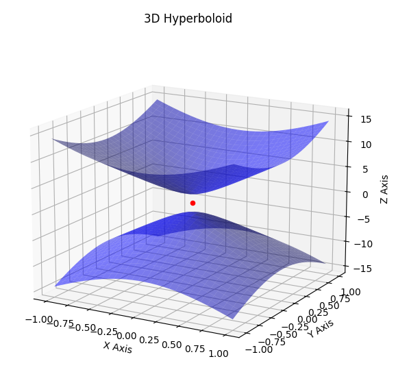
(a)

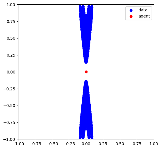
(b)

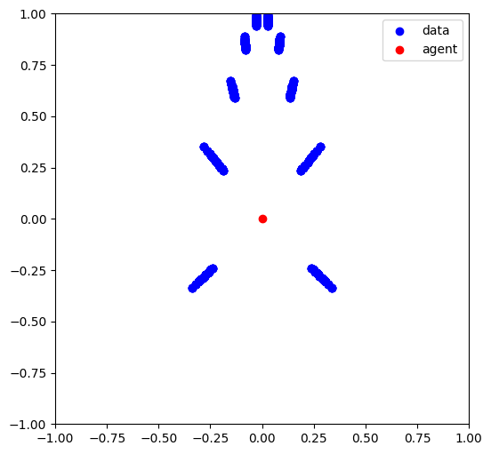
(c)

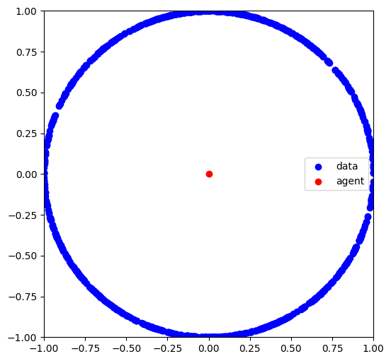
(d)

Figure 10: Examples of cos-MDS on 3 synthetic datasets. The blue points are the synthetic dataset and the red point is the center agent. (a) The 3D hyperboloid dataset; (b) cos-MDS result on the 3D hyperboloid dataset; (c) cos-MDS result on the 4D paraboloid dataset; (d) cos-MDS result on the 4D hypersphere dataset

Appendix C Comparing ESA and Delaunay Triangulation

(a)

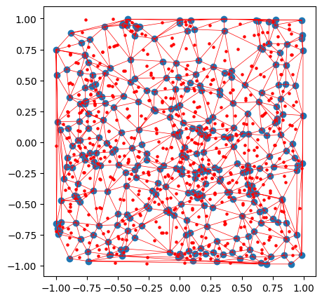
(b)

Figure 11: Given 300 random samples (blue) and 600 random agents (red) in 2D space, we show the outcomes of empty space search using (a) our empty space search algorithm (ESA) and (b) Delaunay Triangulation (DT).

Our investigation into high-dimensional Delaunay triangulation acceleration and approximation revealed a scarcity of research addressing the exponential complexity increase with dimensionality. Hence, we conducted some experiments to study this topic further. Our empirical findings underscore the computational and storage impracticality of these types of approaches for our purposes, even for datasets as small as 1,000 points, when the number of dimensions exceeds 7. Fig. 11(a) and Fig.11(b) show the empty space search results from our search algorithm (ESA) and from Delaunay Triangulation (DT) in the 2D case, respectively. While both methods identify all the empty spaces, DT requires many more triangles compared to the number of agents used in our ESA. It is this abundance (and complexity) of geometric primitives that limits DT’s scalability to higher dimensions.

Appendix D User-Study Results

The user-study data including user performance, ESA performance, and random sampling performance are listed in Tab. II. The parameters used in this study and comparison experiments were $k=9$, $\sigma=$ mean distance of $k$ neighbors, $n=400$, $\alpha=0.001$, $j=10$, $\delta=10^{-7}$, and $\gamma=0.9$, respectively.

TABLE II: Rewards of each round of our user study (top), ESA (middle) and random sampling (below).

User1	User2	User3	User4	User5	User6	User7	User8	User9	User10
0.487	0.4323	0.4317	0.36	0.301	0.368	0.43	0.518	0.287	0.317

ESA1	ESA2	ESA3	ESA4	ESA5	ESA6	ESA7	ESA8	ESA9	ESA10
0.288	0.329	0.295	0.306	0.283	0.334	0.293	0.412	0.293	0.352

Rand1	Rand2	Rand3	Rand4	Rand5	Rand6	Rand7	Rand8	Rand9	Rand10
0.31	0.326	0.283	0.283	0.284	0.312	0.284	0.292	0.294	0.284

D-A ANOVA of User Study

The ANOVA of user study can be found in Tab. III.

TABLE III: The between-subjects ANOVA (above) and Tukey HSD (below) of user performance with GapMiner (x1) against the two baselines ESA-only (x2) and random samples-only (x3).

Source	DF	SS	Mean Square	F Statistic	P-value
Groups	2	0.052	0.026	9.746	$<$0.001
Error	27	0.073	0.003
Total	29	0.125	0.004

Pair	Diff	SE	Q	CI Bounds	CM	P-value
x1-x2	0.075	0.016	4.555	0.017~0.132	0.058	0.009
x1-x3	0.098	0.016	5.976	0.041~0.156	0.058	$<$0.001
x2-x3	0.023	0.016	1.421	-0.034~0.081	0.058	0.580

D-B System Usability Scale

The SUS questionnaire included the 10 questions listed below:

• I think that I would like to use this system frequently.

• I found the system unnecessarily complex.

• I thought the system was easy to use.

• I think that I would need the support of a technical person to be able to use this system.

• I found the various functions in this system were well integrated.

• I thought there was too much inconsistency in this system.

• I would imagine that most people would learn to use this system very quickly.

• I found the system very cumbersome to use.

• I felt very confident using the system.

• I needed to learn a lot of things before I could get going with this system

Each question was ranked from 1 (strongly disagree) to 5 (strongly agree). The final score was calculated by summing the normalized scores and multiplying them by 2.5 to convert the original score of 0-40 to 0-100. 5 users responded to our questionnaire. The results are given in Tab. IV.

TABLE IV: Responses from 5 users. Q1–Q10 refer to 10 questions; R1–R5 refer to user responses. NS in the last row is the normalized score over 5 responses.

Resp	Q1	Q2	Q3	Q4	Q5	Q6	Q7	Q8	Q9	Q10
R1	3	2	4	2	4	2	4	2	4	3
R2	5	1	4	4	5	1	2	2	4	3
R3	5	2	3	2	3	1	4	2	5	4
R4	2	3	4	4	5	1	5	3	4	4
R5	4	1	4	2	5	1	5	1	5	3
NS	2.8	3.2	2.8	2.2	3.4	3.8	3	3	3.4	1.6

D-C Comparison Experiment Data

Fig. 12 presents detailed results achieved by ESA, random sampling and random walk.

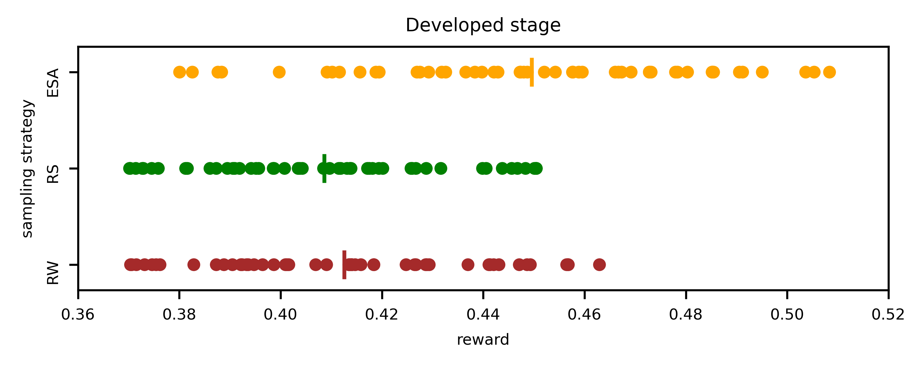
(a)

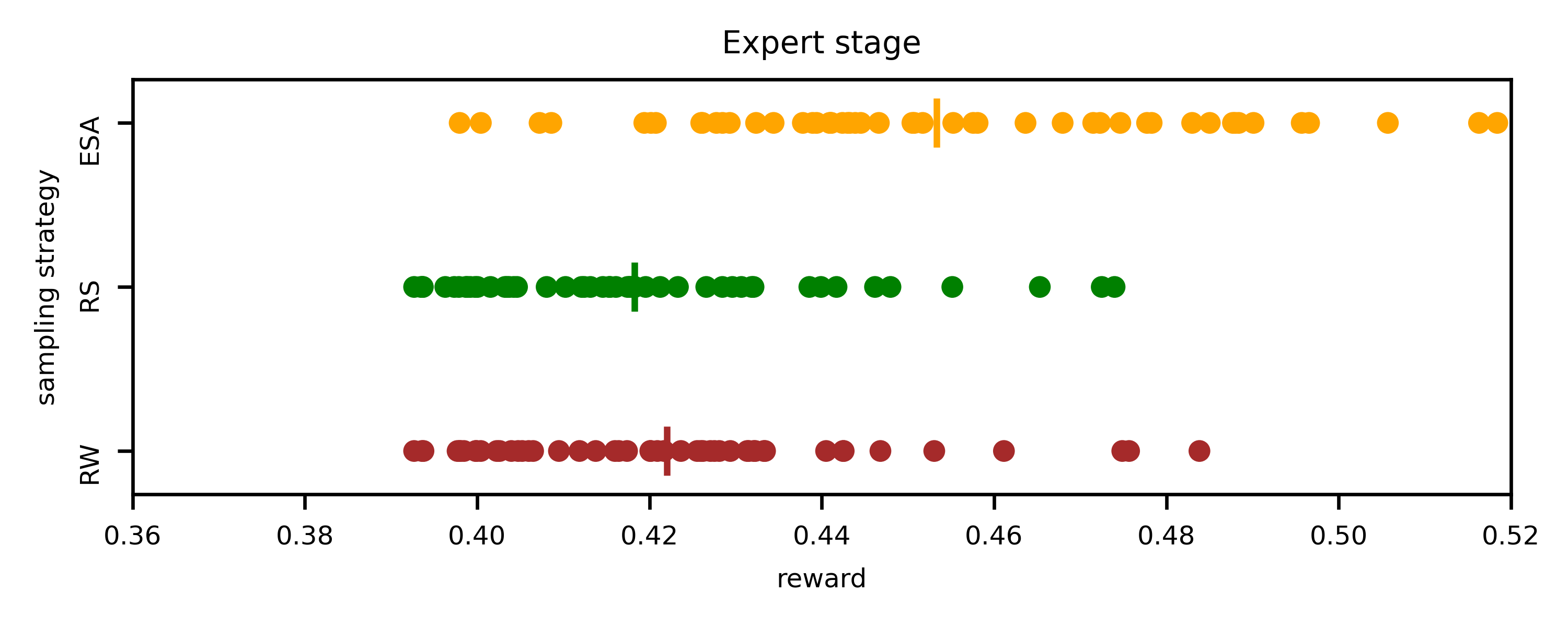
(b)

Figure 12: Comparison experiment: (a) shows the rewards found by ESA, random walk, and random sampling at the development stage; (b) shows the rewards found by the three methods at the expert stage. In both figures, each dot represents a search process with 1,500 random agents involved. Each method in both stages has 50 search processes.

D-D ANOVA of Comparison Experiments

The ANVOA of developed stage and expert stage can be found in Tab. V and Tab. VI respectively.

TABLE V: The within-subjects ANOVA (above) and Tukey HSD (below) of ESA (x1), RS (x2), and RW (x3) at a developed stage. Subjects are the initial positions of agents, Treatments are the empty space search methods.

Source	DF	SS	MS	F Statistic	P-value
Between Subjects	49	0.042	0.001	1.115 (49,98)	0.320
Between Treatments	2	0.051	0.026	33.224 (2,98)	$<\mathbf{10^{-6}}$
Error	98	0.075	0.001
Total	149	0.168	0.001

Pair	Diff	SE	Q	CI Bounds	CM	P-value
x1-x2	0.041	0.004	10.250	0.028~0.054	0.013	$<\mathbf{10^{-6}}$
x1-x3	0.037	0.004	9.272	0.024~0.050	0.013	$<\mathbf{10^{-6}}$
x2-x3	0.004	0.004	0.979	-0.009~0.017	0.013	0.769

TABLE VI: The within-subjects ANOVA (above) and Tukey HSD (below) of ESA (x1), RS (x2), and RW (x3) at an expert stage. Subjects are the initial positions of agents, Treatments are the empty space search methods.

Source	DF	SS	MS	F Statistic	P-value
Between Subjects	49	0.033	0.001	1.201 (49,98)	0.220
Between Treatments	2	0.037	0.019	33.233 (2,98)	$\mathbf{<10^{-6}}$
Error	98	0.055	0.001
Total	149	0.125	0.001

Pair	Diff	SE	Q	CI Bounds	CM	P-value
x1-x2	0.035	0.003	10.161	0.024~0.047	0.012	$\mathbf{<10^{-6}}$
x1-x3	0.031	0.003	9.082	0.020~0.043	0.012	$\mathbf{<10^{-6}}$
x2-x3	0.004	0.003	1.079	-0.008~0.015	0.012	0.726

Appendix E Extrapolation Behavior of Our ESA-Based Search

Our ESA focuses on identifying empty spaces within the data distribution. The repulsive component prevents it from straying too far from the existing distribution. However, empty spaces outside the current distribution can be meaningful and essential. This experiment demonstrates ESA’s ability to search for these empty spaces beyond the current distribution.

We used the distribution of the wine dataset for demonstration; we ignored the meaning of each variable and removed the target variable to focus solely on the distribution of the dataset in each dimension. This marked the dataset as the initial distribution. We ran ESA for six iterations, selecting 300 data items from the dataset with the largest average distance to their 8 nearest neighbors as the initial agent position. ESA search was conducted, and the results were added to the dataset. After each iteration, we measured the distance of the ESA results from the initial distribution and created a histogram. The histograms, shown in Fig. 13, indicate that the configurations found by ESA progressively move further from the initial distribution. This demonstrated ESA’s ability to explore empty spaces beyond an initial data distribution.

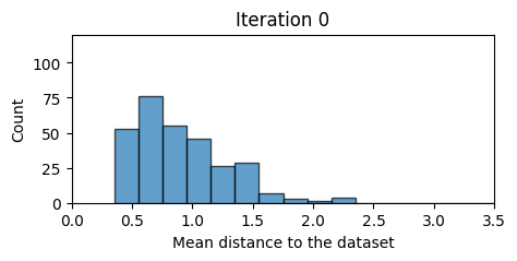
(a)

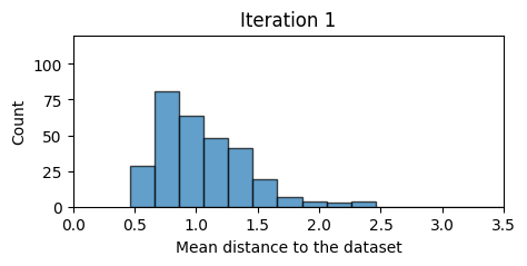
(b)

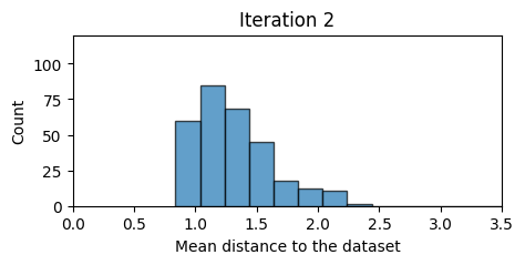
(c)

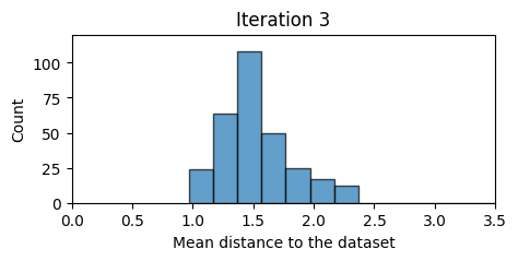
(d)

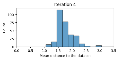
(e)

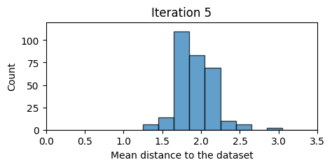
(f)

Figure 13: Histograms of the configurations identified by the ESA with regards to the initial distribution as a function of iteration. We observe that the ESA results progressively move further from the initial distribution, demonstrating ESA’s ability to explore empty spaces beyond an initial data distribution.

Appendix F Details for the Application Cases

In this section we present more detail on the various application examples shown in the paper.

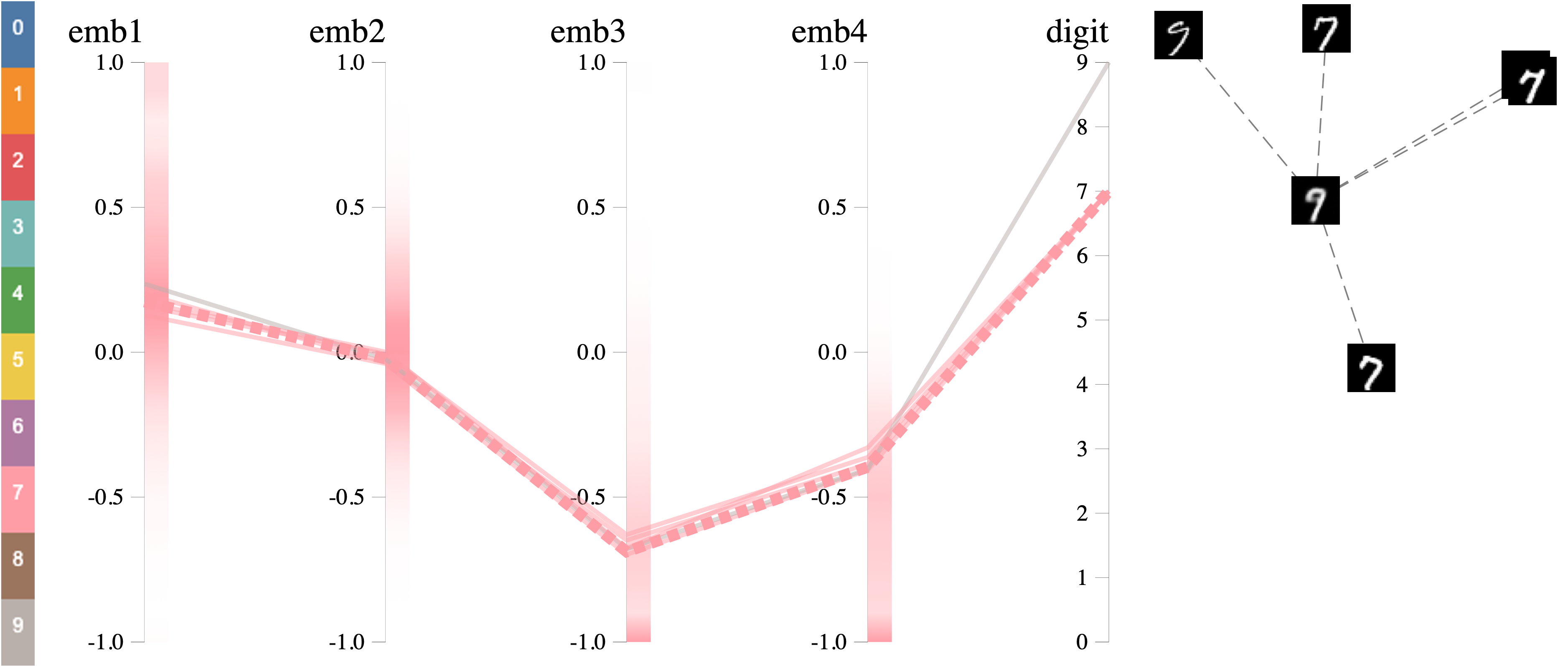
(a)

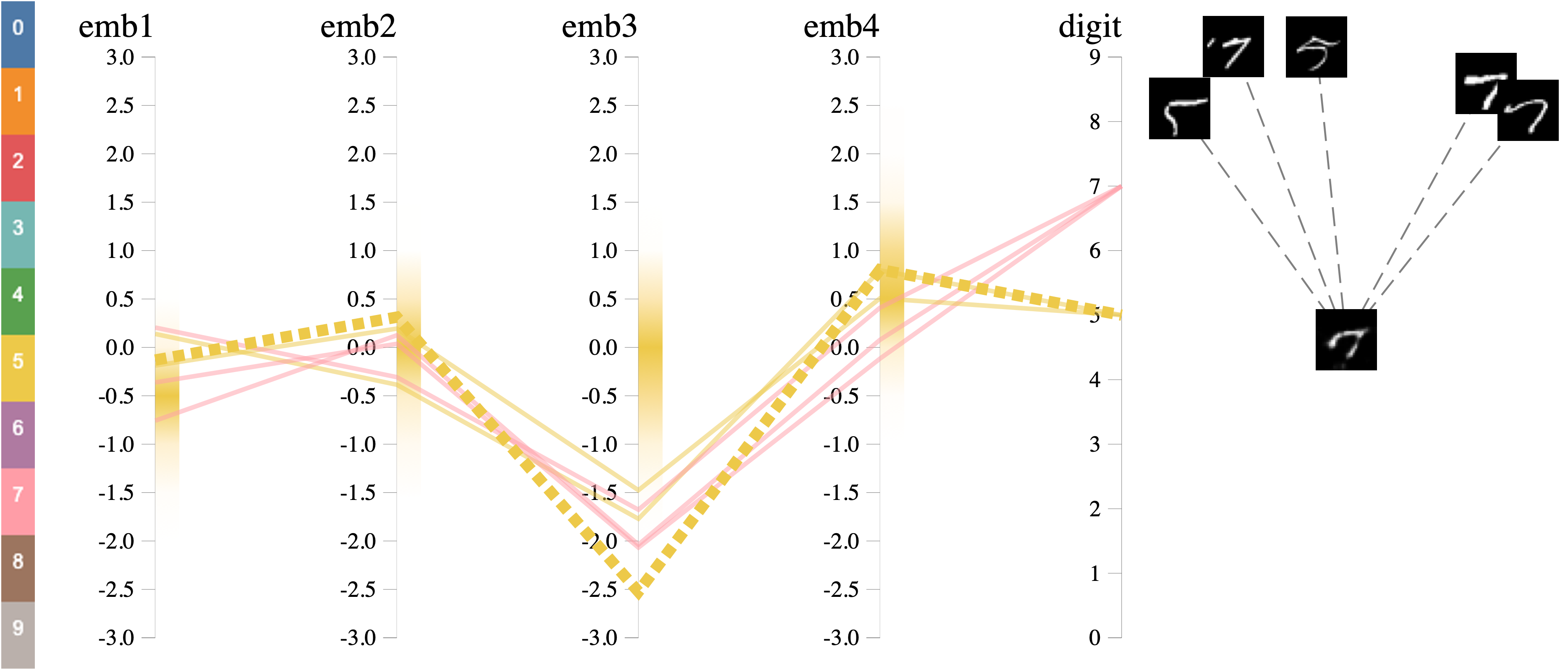
(b)

Figure 14: Some key results from GapMiner. Fig. 9 shows the corresponding PCA map. The leftmost color bar is the legend, where each color represents a digit. The dashed line in the PCP is the empty-space image and the solid lines are its neighbors from MNIST. The line color refers to the true label of images from MNIST or the predicted label of the empty-space image. On the right is the neighbor plot, where the center is the empty-space image (dashed line in the PCP) and around it are the MNIST neighbors (solid lines in the PCP).

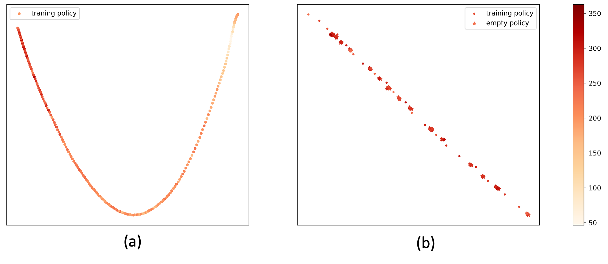
Figure 15: Policy networks visualized by PCA. The color encodes the policy’s return averaged over 10 episodes. (a) Policy checkpoints from all the training iterations. Each point represents one training policy at a checkpoint. (b) Empty space policies and their neighbor training policies. Here, points represent training policies and stars represent empty ones. This is a local space of the last 20 training policies (the top left corner in (a)) since the empty-space policies were identified among the last 20.

F-A Systems Dataset

Fig. 16 shows the full view of GapMiner for the application example described in Fig. VII, the systems dataset.

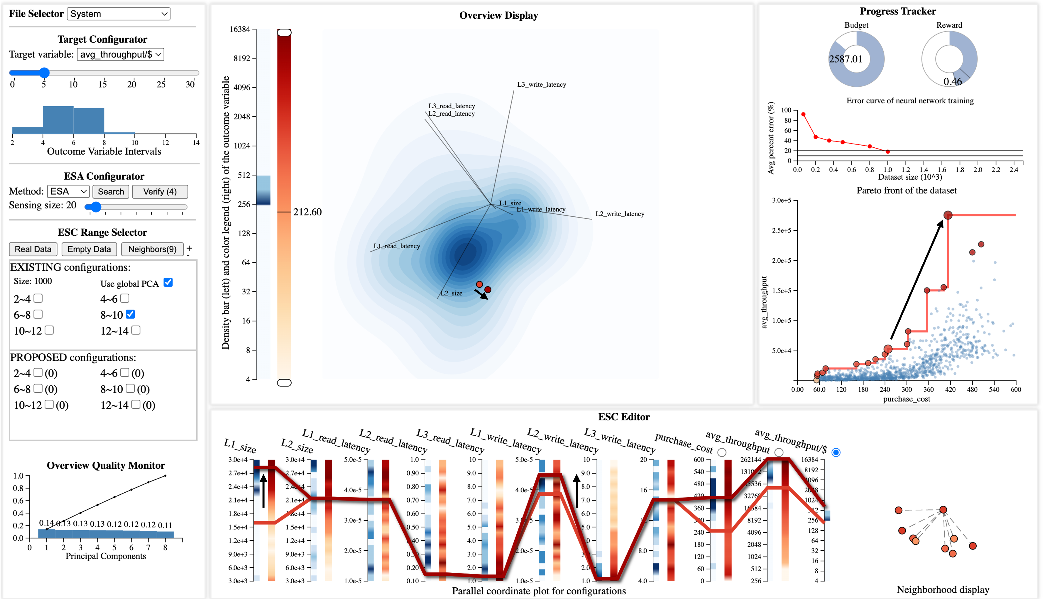
Figure 16: The full view of GapMiner for the system dataset. The black arrows in the overview display, the PCP, and the Pareto frontier plot show the direction of optimization.

F-B Wine Investigation

Fig. 17 show the full view of GapMiner for the wine dataset.

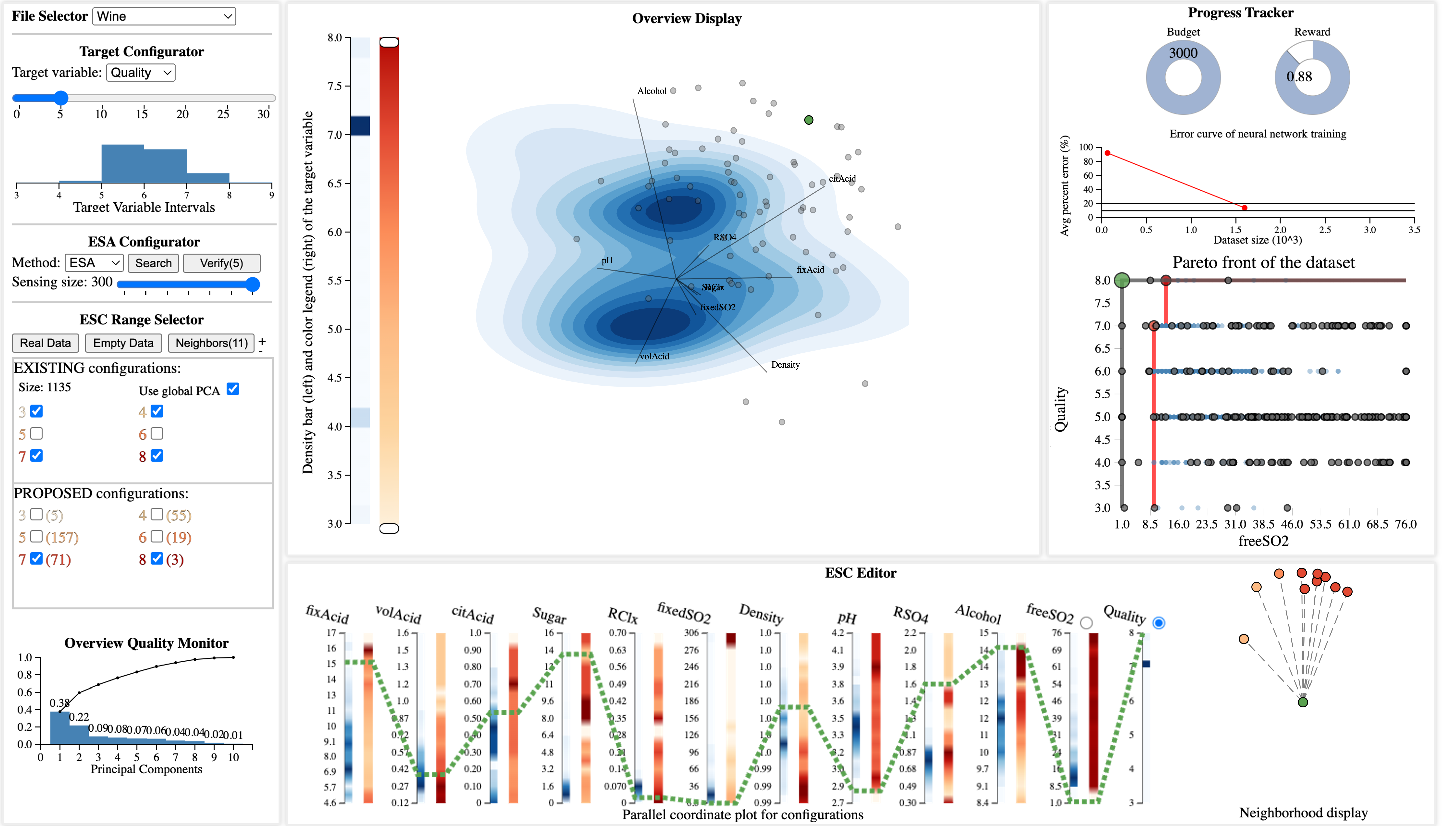
Figure 17: The full view of GapMiner for the wine dataset study. We highlight the global optimal wine instance in green in the PCA map, the PCP, and the neighbor plot.

F-C Empty Space Images in Adversarial Learning

Our first step was to choose relevant digit classes from the control panel and learn the distribution in latent space by using the PCA map and the PCP. With this in hand, we explored the latent space by manipulating a line in the PCP. When the latent point moves in the PCA map, we reconstructed the image with the decoder and visualized it in the neighbor plot. Fig. 14(a) shows an example of the empty-space exploration. Starting from a digit 7, we can see that all of its neighbor images are 7 except one 9, and all are close to the empty space image (dashed line). Changing the image a bit in the latent space results in a shallow line at the head, making it a 9, but the CNN fails to recognize it, still classifying it as a 7. Fig. 14(b) shows another adversarial image by ESA, which is a 7 misclassified as a 5.

Additionally, from Fig. 9(b) we can see that tSNE can correctly embed an adversarial image from Fig. 14(a) into cluster 9 (the pink circle in cluster 9), but it fails for the image from Fig. 14(b) (the yellow circle in cluster 5).

F-D Empty-Space Search in Reinforcement Learning

We visualize the training policies in the PCA space in Fig. 15(a), and the empty-space policies in the PCA space in Fig. 15(b).

F-E Cheetah Direction

We demonstrate an additional application of GapMiner in a physical-simulation scenario.

CheetahDir is an environment in MUJOCO that controls a half cheetah robot to move forward. The reward function is composed of two components: forward reward and control cost. Forward reward is the velocity in the given direction, the faster the better. Control cost is the rooted squared sum of the action, indicating the cost to execute the action, the smaller the better. The total reward is the forward reward minus the control cost. The action space has 6 variables: back thigh, back shin, back foot, front thigh, front shin and front foot. All of them are numerical and continuous.

The dataset is collected by an expert agent. Given an observation, it samples actions from its output distribution randomly. In this scenario, we explored the ability to find better empty space actions than the expert agent given the observation. The visual analytics can be found in Fig. 18.

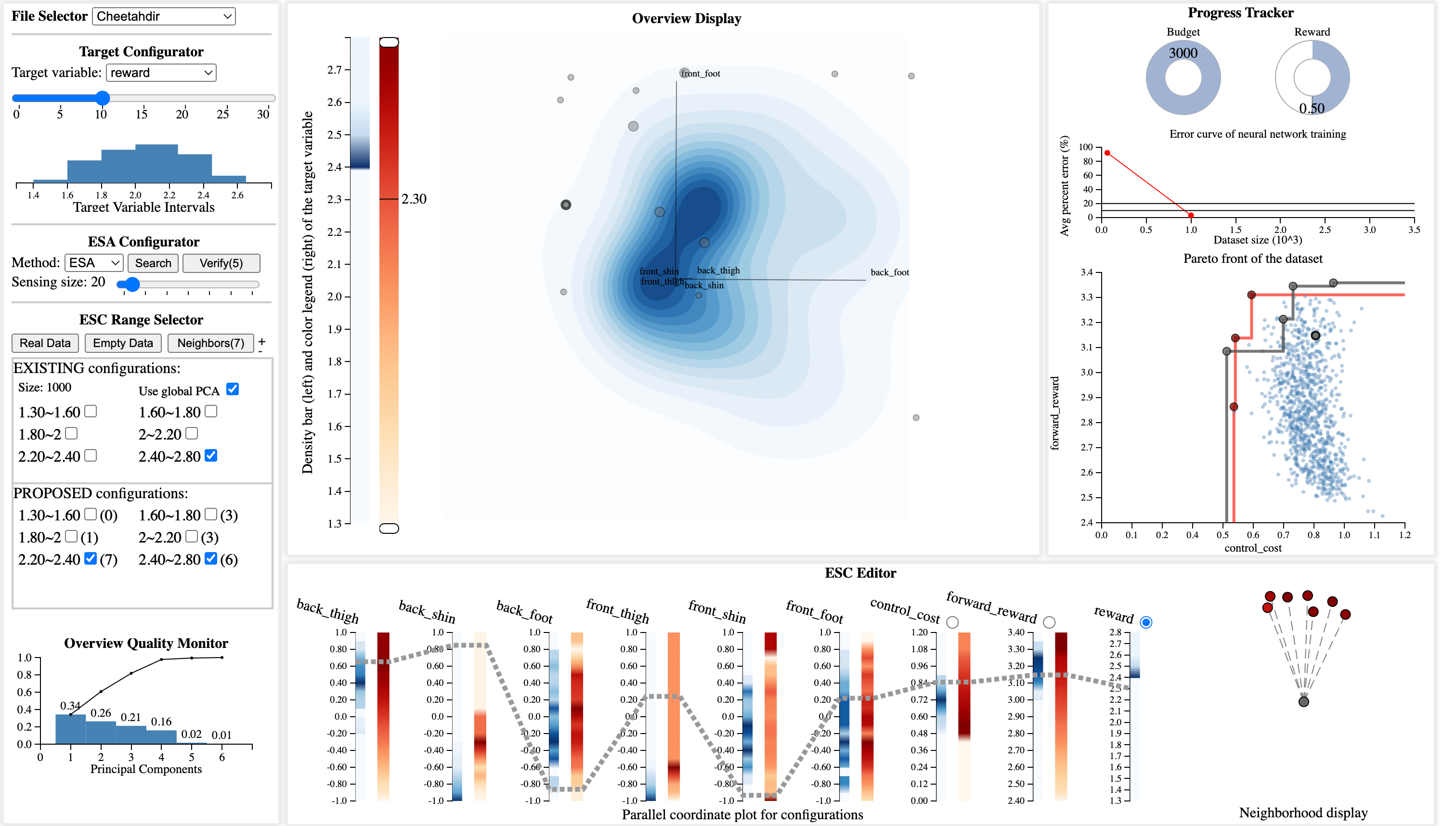
Figure 18: We trained a neural network to predict forward reward and calculate the control cost; then we calculate the reward of an action as forward reward minus control cost. We applied the dataset to GapMiner, from which we could see a distribution shift from low-reward actions to high-reward actions. It indicated that front foot and back foot are more important to the reward. Then we ran ESA to search empty-space actions and plot the predicted forward reward and control cost in the Pareto plot. It showed that actions from the expert agent always have high cost, but some don’t have high reward. ESA can find actions that are either cheaper while maintaining good reward, or expensive but even higher reward. Notice that RL is a sequential decision-making problem. A high immediate reward doesn’t necessarily imply a long-term benefit. Searching empty-space actions with higher Q values is another interesting application scenario.

References

- [1] Rameen Abdal, Yipeng Qin and Peter Wonka “Image2StyleGAN: How to Embed Images Into the StyleGAN Latent Space?” In Proc. ICCV, 2019, pp. 4432–4441
- [2] Omid Alipourfard et al. “CherryPick: Adaptively unearthing the best cloud configurations for big data analytics” In USENIX Symposium on Networked Systems Design and Implementation, 2017, pp. 469–482
- [3] Randall Balestriero, Zichao Wang and Richard Baraniuk “DeepHull: Fast Convex Hull Approximation in High Dimensions” In ICASSP, 2022, pp. 3888–3892
- [4] Aaron Bangor, Philip Kortum and James Miller “Determining What Individual SUS Scores Mean: Adding an Adjective Rating Scale” In Journal of Usability Studies 4.3 Usability Professionals’ Association Bloomingdale, IL, 2009, pp. 114–123
- [5] Richard Bellman “Dynamic Programming” In Science 153.3731 American Association for the Advancement of Science, 1966, pp. 34–37
- [6] Rongzheng Bian et al. “Implicit Multidimensional Projection of Local Subspaces” In IEEE Transactions on Visualization and Computer Graphics 27.2 IEEE, 2020, pp. 1558–1568
- [7] Guy Blelloch, Gary Miller, Jonathan Hardwick and Dafna Talmor “Design and Implementation of a Practical Parallel Delaunay Algorithm” In Algorithmica 24, 1999, pp. 243–269
- [8] John Brooke “SUS: A ‘Quick and Dirty’ Usability Scale” In Usability Evaluation in Industry 189, 1995
- [9] Steven Brunton “Data-driven aerospace engineering: reframing the industry with machine learning” In AIAA Journal 59.8, 2021, pp. 2820–2847
- [10] Yongtao Cao, Byran Smucker and Timothy Robinson “On Using the Hypervolume Indicator to Compare Pareto Fronts: Applications to Multi-criteria Optimal Experimental Design” In Journal of Statistical Planning and Inference 160, 2015, pp. 60–74
- [11] Nitesh Chawla, Kevin Bowyer, Lawrence Hall and W. Kegelmeyer “SMOTE: Synthetic Minority Over-sampling Technique” In Journal of Artificial Intelligence Research 16, 2002, pp. 321–357
- [12] Jie Chen and Yongming Liu “Neural Optimization Machine: A Neural Network Approach for Optimization” In arXiv preprint arXiv:2208.03897, 2022
- [13] Jingdi Chen, Tian Lan and Nakjung Choi “Distributional-Utility Actor-Critic for Network Slice Performance Guarantee” In Proc. International Symposium on Theory, Algorithmic Foundations, and Protocol Design for Mobile Networks and Mobile Computing, 2023, pp. 161–170
- [14] Jingdi Chen et al. “Real-Time Network Intrusion Detection via Decision Transformers” In arXiv preprint arXiv:2312.07696, 2023
- [15] Shenghui Cheng and Klaus Mueller “The Data Context Map: Fusing Data and Attributes into a Unified Display” In IEEE Transactions on Visualization and Computer Graphics 22.1 IEEE, 2015, pp. 121–130
- [16] Raffaele Cioffi et al. “Artificial intelligence and machine learning applications in smart production: Progress, trends, and directions” In Sustainability 12.2 MDPI, 2020, pp. 492
- [17] Jacob Cohen, Patricia Cohen, Stephen West and Leona Aiken “Applied Multiple Regression/Correlation Analysis for the Behavioral Sciences” Routledge, 2013
- [18] Mark De Berg “Computational Geometry: Algorithms and Applications” Springer Science & Business Media, 2000
- [19] Sumeyra Demir, Bart Stappers, Koen Kok and Nikolaos Paterakis “Statistical Arbitrage Trading on the Intraday Market Using the Asynchronous Advantage Actor–Critic Method” In Applied Energy 314 Elsevier, 2022, pp. 118912
- [20] Geoffrey Ellis and Alan Dix “A Taxonomy of Clutter Reduction for Information Visualisation” In IEEE Transactions on Visualization and Computer Graphics 13.6 IEEE, 2007, pp. 1216–1223
- [21] Tyler Estro et al. “Accelerating Multi-Tier Storage Cache Simulations Using Knee Detection” In Performance Evaluation, 2024, pp. 102410
- [22] Tyler Estro, Pranav Bhandari, Avani Wildani and Erez Zadok “Desperately Seeking … Optimal Multi-Tier Cache Configurations” In HotStorage, 2020
- [23] Joachim Giesen, Lars Kühne and Philipp Lucas “Sclow Plots: Visualizing Empty Space” In Computer Graphics Forum 36.3, 2017, pp. 145–155 Wiley Online Library
- [24] Robert Graham and Adam Oberman “Approximate Convex Hulls: sketching the convex hull using curvature” In arXiv preprint arXiv:1703.01350, 2017
- [25] Tuomas Haarnoja, Aurick Zhou, Pieter Abbeel and Sergey Levine “Soft Actor-Critic: Off-Policy Maximum Entropy Deep Reinforcement Learning with a Stochastic Actor” In ICML, 2018, pp. 1861–1870
- [26] Sariel Har-Peled “A Replacement for Voronoi Diagrams of Near Linear Size” In IEEE Symp. on Foundations of Computer Science, 2001, pp. 94–103
- [27] Harold Hotelling “Analysis of a complex of statistical variables into principal components.” In Journal of Educational Psychology 24.6 Warwick & York, 1933, pp. 417
- [28] Frank Hutter, Holger H. Hoos and Thomas Stützle “Automatic Algorithm Configuration based on Local Search” In AAAI 7, 2007, pp. 1152–1157
- [29] Alfred Inselberg “The plane with parallel coordinates” In The Visual Computer 1 Springer, 1985, pp. 69–91
- [30] Luis Japa et al. “A Population-Based Hybrid Approach for Hyperparameter Optimization of Neural Networks” In IEEE Access 11 Institute of ElectricalElectronics Engineers (IEEE), 2023, pp. 50752–50768 DOI: 10.1109/access.2023.3277310
- [31] Tero Karras, Samuli Laine and Timo Aila “A Style-Based Generator Architecture for Generative Adversarial Networks” In CVPR, 2019, pp. 4401–4410
- [32] Emre Kıcıman, Robert Ness, Amit Sharma and Chenhao Tan “Causal Reasoning and Large Language Models: Opening a New Frontier for Causality” In arXiv preprint arXiv:2305.00050, 2023
- [33] Vijay Konda and John Tsitsiklis “Actor-Critic Algorithms” In NeurIPS 12, 1999
- [34] Hans-Peter Kriegel, Peer Kröger and Arthur Zimek “Subspace Clustering” In Wiley Interdisciplinary Reviews: Data Mining and Knowledge Discovery 2.4 Wiley Online Library, 2012, pp. 351–364
- [35] J. Lennard and I. Jones “On the Determination of Molecular Fields.–—I. From the Variation of the Viscosity of a Gas with Temperature” In Proceedings of the Royal Society of London. Series A 106.738, 1924, pp. 441–462
- [36] Harry Li, Steven Jorgensen, John Holodnak and Allan Wollaber “ScatterUQ: Interactive Uncertainty Visualizations for Multiclass Deep Learning Problems” In IEEE VIS, 2023, pp. 246–250
- [37] Heyi Li et al. “Transforming the Latent Space of StyleGAN for Real Face Editing” In The Visual Computer Springer, 2023, pp. 1–16
- [38] Lanqing Li et al. “Towards an Information Theoretic Framework of Context-Based Offline Meta-Reinforcement Learning” In arXiv preprint arXiv:2402.02429, 2024
- [39] Mats Lind, Jimmy Johansson and Matthew Cooper “Many-to-Many Relational Parallel Coordinates Displays” In IEEE InfoVis, 2009, pp. 25–31
- [40] Helena Lourenço, Olivier Martin and Thomas Stützle “Iterated Local Search” In Handbook of Metaheuristics Springer, 2003, pp. 320–353
- [41] Salman Mahmood and Klaus Mueller “Interactive Subspace Cluster Analysis Guided by Semantic Attribute Associations” In IEEE Transactions on Visualization and Computer Graphics IEEE, 2023
- [42] Kevin T. McDonnell and Klaus Mueller “Illustrative Parallel Coordinates” In Computer Graphics Forum 27.3, 2008, pp. 1031–1038 Wiley Online Library
- [43] Leland McInnes, John Healy and James Melville “Umap: Uniform Manifold Approximation and Projection for Dimension Reduction” In arXiv preprint arXiv:1802.03426, 2018
- [44] Al Mead “Review of the Development of Multidimensional Scaling Methods” In Journal of the Royal Statistical Society: Series D 41.1 Wiley Online Library, 1992, pp. 27–39
- [45] Eduardo Mosqueira-Rey et al. “Human-in-the-loop machine learning: a state of the art” In Artificial Intelligence Review 56.4 Springer, 2023, pp. 3005–3054
- [46] Tamara Munzner “A Nested Model for Visualization Design and Validation” In IEEE Trans. Visualization and Computer Graphics 15.6 IEEE, 2009, pp. 921–928
- [47] Cuong Nguyen and Philip Rhodes “Delaunay Triangulation of Large-Scale Datasets Using Two-Level Parallelism” In Parallel Computing 98 Elsevier, 2020, pp. 102672
- [48] Gregorio Palmas et al. “An Edge-Bundling Layout for Interactive Parallel Coordinates” In 2014 IEEE Pacific Visualization Symposium, 2014, pp. 57–64 IEEE
- [49] Jack Parker-Holder, Vu Nguyen and Stephen J Roberts “Provably Efficient Online Hyperparameter Optimization with Population-Based Bandits” In Advances in Neural Information Processing Systems 33 Curran Associates, Inc., 2020, pp. 17200–17211 URL: https://proceedings.neurips.cc/paper_files/paper/2020/file/c7af0926b294e47e52e46cfebe173f20-Paper.pdf
- [50] Milos Radovanovic, Alexandros Nanopoulos and Mirjana Ivanovic “Hubs in Space: Popular Nearest Neighbors in High-Dimensional Data” In Journal of Machine Learning Research 11, 2010, pp. 2487–2531
- [51] Sam Roweis and Lawrence Saul “Nonlinear Dimensionality Reduction by Locally Linear Embedding” In Science 290.5500 American Association for the Advancement of Science, 2000, pp. 2323–2326
- [52] Salah Sammari “red wine data” Accessed on 2024-02-01, https://www.kaggle.com/datasets/midouazerty/redwine
- [53] Jeff Sauro “A Practical Guide to the System Usability Scale: Background, Benchmarks & Best Practices” Measuring Usability LLC, 2011
- [54] Raimund Seidel “The upper bound theorem for polytopes: an easy proof of its asymptotic version” In Computational Geometry 5.2 Elsevier, 1995, pp. 115–116
- [55] Ondřej Strnad, Vilém Šustr, Barbora Kozlíková and Jiří Sochor “Real-Time Visualization of Protein Empty Space with Varying Parameters” In Proc, of BIOTECHNO, IARIA XPS Press, 2013, pp. 65–70
- [56] Andrada Tatu et al. “ClustNails: Visual analysis of subspace clusters” In Tsinghua Science and Technology 17.4 TUP, 2012, pp. 419–428
- [57] Emanuel Todorov, Tom Erez and Yuval Tassa “MuJoCo: A physics engine for model-based control” In IEEE/RSJ International Conference on Intelligent Robots and Systems, 2012, pp. 5026–5033
- [58] Laurens Van der Maaten and Geoffrey Hinton “Visualizing Data Using t-SNE” In Journal of Machine Learning Research 9.11, 2008
- [59] Gabriel Villarrubia, Juan De Paz, Pablo Chamoso and Fernando De la Prieta “Artificial neural networks used in optimization problems” In Neurocomputing 272, 2018, pp. 10–16
- [60] Carl Waldspurger, Nohhyun Park, Alexander Garthwaite and Irfan Ahmad “Efficient MRC Construction with SHARDS” In FAST, 2015, pp. 95–110
- [61] Bing Wang and Klaus Mueller “The Subspace Voyager: Exploring High-Dimensional Data along a Continuum of Salient 3D Subspaces” In IEEE Transactions on Visualization and Computer Graphics 24.2 IEEE, 2017, pp. 1204–1222
- [62] Junpeng Wang, Xiaotong Liu and Han-Wei Shen “High-dimensional data analysis with subspace comparison using matrix visualization” In Information Visualization 18.1 SAGE Publications Sage UK: London, England, 2019, pp. 94–109
- [63] Sushen Zhang, Seyed Bamakan, Qiang Qu and Sha Li “Learning for personalized medicine: a comprehensive review from a deep learning perspective” In IEEE Reviews in Biomedical Engineering 12, 2018, pp. 194–208
- [64] Xinyu Zhang, Shenghui Cheng and Klaus Mueller “Graphical Enhancements for Effective Exemplar Identification in Contextual Data Visualizations” In IEEE Transactions on Visualization and Computer Graphics IEEE, 2022
- [65] Yanming Zhang et al. “An Explainable AI Approach to Large Language Model Assisted Causal Model Auditing and Development” In arXiv preprint arXiv:2312.16211, 2023
- [66] Arthur Zimek, Erich Schubert and Hans-Peter Kriegel “A Survey on Unsupervised Outlier Detection in High-Dimensional Numerical Data” In Statistical Analysis and Data Mining: The ASA Data Science Journal 5.5 Wiley Online Library, 2012, pp. 363–387