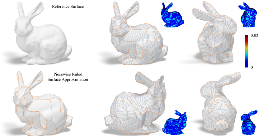
Figure 1. Piecewise ruled surface approximation computed using our method. The sub-figures on the right show different views of the result surface together with the rulings. We also use color coding to visualize the distance from the result surface to the reference surface, normalized by the reference surface’s bounding box diagonal length.

Piecewise Ruled Approximation for Freeform Mesh Surfaces

Abstract.

A ruled surface is a shape swept out by moving a line in 3D space. Due to their simple geometric forms, ruled surfaces have applications in various domains such as architecture and engineering. However, existing methods that use ruled surfaces to approximate a target shape mainly focus on surfaces of non-positive Gaussian curvature. In this paper, we propose a method to compute a piecewise ruled surface that approximates an arbitrary freeform surface. Given the input shape represented as a triangle mesh, we propose a group-sparsity formulation to optimize the mesh shape into an approximately piecewise ruled form, in conjugation with a tangent vector field that indicates the ruling directions. Afterward, we use the optimization result to extract the patch topology and construct the initial rulings. Finally, we further optimize the positions and orientations of the rulings to improve the alignment with the input target shape. We apply our method to a variety of freeform shapes with different topologies and complexity, demonstrating its effectiveness in approximating arbitrary shapes.

1. Introduction

Freeform surfaces are widely used in various application domains, including computer-aided design, architecture, and manufacturing. However, the fabrication of these surfaces often poses significant challenges due to their complex geometry. One common approach to simplify the realization of freeform surfaces is to approximate them with surface elements with simple shapes. In this paper, we investigate freeform surface approximation using piecewise ruled surfaces. Ruled surfaces are swept out by a continuous family of straight lines in 3D space. They can be parameterized by a correspondence between two curves $\mathbf{b}_{1}(v)$ and $\mathbf{b}_{2}(u)$:

(1) $$\mathbf{p}(u,v)=(1-v)\mathbf{b}_{1}(u)+v\mathbf{b}_{2}(u),$$

where points with the same $u$ value are on a straight line connecting the two curves. Alternatively, they can be represented as moving a straight line along a curve $\mathbf{a}(u)$:

(2) $$\mathbf{p}(u,v)=\mathbf{a}(u)+v\mathbf{r}(u),$$

where $\mathbf{r}(u)$ is the line direction at point $\mathbf{a}(u)$. The constituent straight lines on a ruled surface are called rulings. The simple geometric form of ruled surfaces enables them to effectively approximate freeform shapes while allowing for efficient fabrication, e.g., by arranging straight elements such as tensioned strings (see Fig. 2) or using straight line motions of CNC tools like 5-axis side milling.

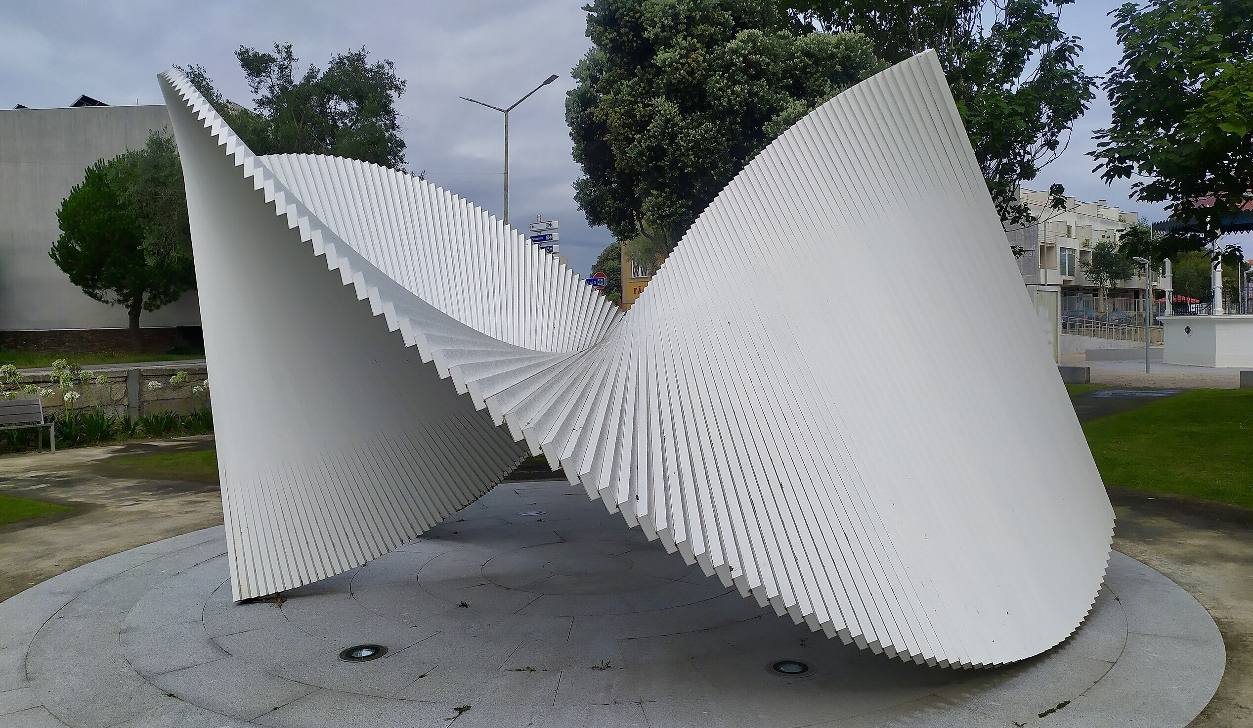
Figure 2. Examples of ruled surfaces. Top: an art installation using tensioned strings, in the Science Museum in London. Bottom: a sculpture by Ascânio MMM, in Fão, Esposende, Portugal.

In the past, numerous research efforts have been devoted to piecewise approximation using developable patches, a special type of ruled surfaces with a constant zero Gaussian curvature (Kilian et al., 2008; Tang et al., 2016; Stein et al., 2018; Ion et al., 2020; Zhao et al., 2022, 2023). However, investigation into approximation using general ruled surfaces—which allow for non-positive Gaussian curvature and offer more degrees of freedom than developable surfaces for better approximation—has been limited. Existing methods have primarily focused on target surfaces represented in parametric forms (1997; 2014) or require the target surface to have non-positive Gaussian curvature everywhere (Flöry et al., 2013). This limitation restricts their applicability to a broader range of freeform surfaces that arise in real-world applications, such as those represented as triangle meshes and containing positive Gaussian curvature regions. In addition, in practical applications, it is preferable to reduce the number of patches used in the approximation for both aesthetics and ease of fabrication. However, an insufficient number of patches may lead to a poor approximation of the target shape because of the limited degrees of freedom for ruled surfaces. It is a challenging problem to determine a suitable patch topology that can achieve good alignment with the target shape while minimizing the number of patches. In this paper, we present a novel approach for computing a piecewise ruled surface that closely approximates an arbitrary given freeform surface with a small number of patches. Our method works on triangle mesh surfaces and can handle surfaces with both positive and negative Gaussian curvature, making it more versatile than previous techniques. We address this problem in three main stages. First, we introduce a new approach that simultaneously optimizes the mesh shape and a ruling direction field on the mesh. Instead of a piecewise constant representation that is commonly used in geometry processing for tangent vector fields, we propose a novel representation of the ruling direction field on mesh surfaces based on its first-order approximation, which better captures the variation of the ruling directions within a local neighborhood. By employing a sparsity-based optimization with this representation, our method produces a piecewise smooth direction field on the updated mesh surface, which serves as an approximation of the final piecewise ruled surface shape and its ruling directions. Our sparsity formulation ensures that the direction field is smooth across most areas on the surface, with a small number of discontinuities that indicate potential patch boundaries, thus helping to reduce the number of resulting patches. Afterward, we construct the initial piecewise ruled surface shape by utilizing the discontinuities of the ruling direction field to determine the patch topology, and by tracing along the direction field to construct initial rulings that connect the patch boundaries. Lastly, we further optimize the patch boundary curves to improve the alignment between the piecewise ruled surface and the target shape while maintaining smoothness. The final output is an explicit representation of the optimized ruled patches’ boundaries and their rulings, ready for downstream applications.

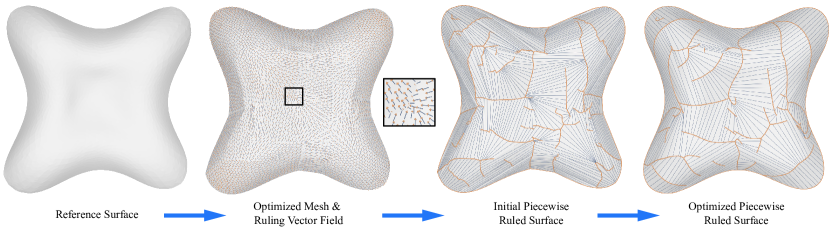
Figure 3. The pipeline of our piecewise ruled surface approximation. Given an input reference surface mesh, we first optimize the mesh shape together with a vector field on it, to approximate a piecewise ruled surface and its rulings. The result is then used to extract an initial piecewise ruled surface. Lastly, we optimize the piecewise ruled surface to further align it with the reference surface and obtain the final result.

Extensive experiments demonstrate that our method can effectively construct piecewise ruled surface shapes that accurately approximate various target freeform surfaces with a small number of patches, outperforming existing approaches in terms of both accuracy and versatility. In summary, the main contributions of this paper include:

• A novel representation of ruling direction fields on mesh surfaces, which better captures their local variations than the canonical piecewise constant representation and enables more effective optimization of the ruling direction.

• A sparsity-based formulation for the joint optimization of the mesh shape and the ruling direction field on the mesh, providing a reliable approximation of the final piecewise ruled surface while reducing the number of its patches.

• A topology extraction method that utilizes the optimized direction field to determine the layout of the ruled surface patches and initialize their ruling directions, facilitating further optimization to align the piecewise ruled surface with the target shape.

2. Related Work

Ruled surface approximation and developable surface approximation have been extensively studied in computer graphics and computer-aided design. We review the most relevant papers in the following.

Ruled Surface Approximation

Elber and Fish (1997) construct a piecewise ruled approximation of freeform surfaces using Bézier surfaces and a subdivision scheme to meet a given error tolerance, but do not guarantee global accessibility of the surface by the cutting tool. Chen and Pottmann (1999) present a method to approximate a given surface or scattered points with a ruled surface in tensor-product B-spline representation, using a three-step process of finding discrete rulings, constructing an approximating B-spline ruled surface, and optional final fitting. Han et al. (2001) introduce an isophote-based piecewise ruled surface approximation method that adapts to surface features and investigate its application in 5-axis NC rough and finish machining using tapered cutting tools. Flöry et al. (2013) investigate using ruled surface strips to approximate architectural freeform surfaces, focusing on smoothness between rulings and identifying areas where a good rationalization can be achieved. Wang and Elber (2014) use GPU-based dynamic programming to minimize the distance between the original surface and the rationalization. Steenstrup et al. (2016) propose an algorithm to approximate a given surface with a piecewise ruled surface that never intersects the original surface and is cuttable by wire cutting, which can be used as a pre-processing step before milling. Hua and Jia (2018) present a method for producing double-sided minimal surfaces by wire-cut machines, using Weierstrass parameterization and principal curvature directions to plan orthogonal cuts on both sides of the surface.

Developable Surface Approximation

Developable surfaces can be unfolded into the plane, enabling easy fabrication from non-stretchable sheet materials. Modeling and approximation using developable surfaces is a long-standing research problem in computer graphics. Below we briefly review the contributions most related to our method. Mitani and Suzuki (2004) propose a strip-based approximation method that segments the mesh into feature-based parts, groups triangles into zonal regions, and simplifies each part into continuous triangle strips free of internal vertices, allowing the strips to be unfolded into papercraft patterns. Liu et al. (2006) introduce conical meshes as quadrilateral meshes with planar faces that can be naturally offset and aligned with principal curvature networks, facilitating freeform glass structures in architectural design and providing an effective modeling method for developable surfaces. Kilian et al. (2008) propose an optimization-based computational framework for designing and reconstructing surfaces that can be created by curved folding from a single planar sheet, enabling complex forms without stretching or cutting. Tang et al. (2016) represent developables as splines, formulating developability and curved folds as quadratic equations, and employing an energy-guided projection solver and a primal-dual surface representation for efficient interactive modeling. Stein et al. (2018) define a notion of developability for triangle meshes that exactly captures flattenability and straight ruling lines, and propose a variational approach that drives a mesh toward developable patches separated by seam curves without explicit patch clustering. Rabinovich et al. (2018) introduce a discrete approach to modeling developable surfaces as quadrilateral meshes with simple angle constraints, relying on orthogonal geodesics rather than explicit rulings, and enabling local isometric deformations while retaining second-order consistency with smooth counterparts. Jiang et al. (2020) discretize isometric mappings as correspondences between checkerboard patterns derived from quad meshes, allowing a flexible class of discrete developable surfaces that supports isometric and conformal mappings, isometric bending, and a variety of geometric modeling operations including cutting, gluing, and folding. Ion et al. (2020) propose an automatic tool that wraps a given 3D surface with discrete orthogonal geodesic nets, employing a global optimization strategy to place piecewise developable patches, and then applies a nonlinear projection to approximate the input surface with fewer patches for simpler fabrication. Binninger et al. (2021) introduce an iterative method that leverages the 1D nature of the Gauss image, alternating between thinning the Gauss image and deforming the surface to achieve piecewise developable approximations, while preserving mesh connectivity and effectively handling non-developable inputs. Zhao et al. (2022) approximate a triangular mesh with a small set of nearly developable patches by introducing an edge-oriented discrete developability measure and optimizing a developability-encouraged deformation energy. They then partition the deformed mesh into developable patches in a coarse-to-fine manner, deriving a piecewise developable approximation. Later, Zhao et al. (2023) propose a method to compute piecewise developable approximation for triangular meshes using an evolutionary genetic algorithm that optimizes a combinatorial fitness function accounting for approximation error, patch count, patch boundary length, and penalties for small or narrow patches.

3. Method

Given a triangle mesh $\mathcal{M}$ representing a target freeform surface, we would like to approximate its shape using a piecewise ruled surface $\mathcal{S}$; i.e., $\mathcal{S}$ may consist of multiple ruled surface patches joined along their boundaries. We propose a method consisting of three steps (see Fig. 3):

• First, we optimize the vertex positions of $\mathcal{M}$ to deform it into an approximately piecewise ruled surface close to the target shape. A dense vector field on the mesh surface is also jointly optimized to indicate the ruling directions.

• Afterward, we use the optimized mesh and vector field to determine the boundaries between the ruled surface patches, and trace along the vector field to identify the correspondence between points on the boundaries. The corresponding boundary sample points are then connected with straight line segments to form the initial rulings. In this way, the boundary sample points represent both the boundary curves and the rulings, which define the piecewise ruled surface $\mathcal{S}$.

• Lastly, we optimize the boundary sample point positions to further align $\mathcal{S}$ with and the target shape, obtaining the final shape of $\mathcal{S}$.

Details for each step are explained in the following.

3.1. Optimizing Mesh Shape and Ruling Direction Field

Since a ruled surface has limited degrees of freedom and can only have non-positive Gaussian curvature values, a complex target shape often require multiple ruled surface patches to achieve good approximation. Choosing a suitable topology for such a piecewise ruled surface (i.e., the number of patches and their adjacency relation) is crucial for effectively optimizing its shape. However, the appropriate topology depends on the target surface geometry in a highly nonlinear manner and cannot be determined easily. To address this problem, we first optimize the vertex positions of the input mesh $\mathcal{M}$ and a vector field on its surface, such that $\mathcal{M}$ deforms into a shape consisting of multiple approximately ruled regions, where the vector field indicates the ruling directions. The deformed mesh is then used for determining the piecewise ruled surface topology. In this subsection, we explain our formulation for mesh optimization and its numerical solution.

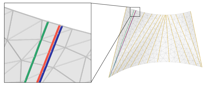
Figure 4. Piecewise constant vector fields are insufficient for capturing the variation of ruling directions on a ruled surface. Here we show a ruled surfce discretized as a triangle mesh, where the original rulings are a smooth family of straight lines connecting the top and bottom curves (a subset is displayed here in brown). We first represent the ruling directions using a piecewise constant vector field according to the original ruling directions at the face centroids, and use it to trace a polyline starting from a point on the bottom boundary. There is a notable deviation between the resulting polyline (displayed in green) and the original ruling starting at the same point (displayed in red) when they reach the top boundary. On the other hand, if we represent the ruling directions with our proposed vector field model (10) and start tracing from the same point, the resulting polyline (displayed in blue) is much closer to the original ruling.

3.1.1. Representation of ruling direction fields

On a smooth ruled surface, the direction vector of a ruling is a member of the tangent space at every point on the ruling. Therefore, we can represent the ruling directions as a tangent vector field on the mesh surface. One popular approach is to use a piecewise-constant vector field, where the vector field on each triangle face has a constant value orthogonal to the face normal (do Goes et al., 2015). However, this conventional approach is not suitable for our problem. In particular, after the mesh optimization, we need to trace along the vector field to derive polylines that approximate the rulings. With a piecewise constant representation, the constant vector field on each face may be insufficient for capturing the variation of ruling directions within the face to allow for accurate tracing of the rulings. One such example is shown in Fig. 4. Here we show a ruled surface discretized as a triangle mesh, where the original rulings are a smooth family of straight lines connecting the upper and lower boundary curves (a subset of the original rulings are shown in brown). We compute a piecewise constant vector field on the mesh to approximate the ruling directions, where the constant vector direction on each face is equal to the projected direction of the original ruling whose projection on the face passes through the face centroid. Then, we start from a point at the bottom curve, and trace a polyline on the mesh (displayed in green) according to the piecewise constant vector field. We also show the original ruling that starts from the same point at the bottom (displayed in red). We can observe a notable deviation between the traced polyline and the original ruling at the top boundary, indicating an insufficient accuracy from the ruling direction approximation using the piecewise constant vector field.

To better approximate the ruling directions, we adopt a different representation based on the following observation. For a point $\mathbf{p}\in\mathbb{R}^{3}$ on a ruled surface $\mathcal{R}$, let $\mathbf{r}_{\mathbf{p}}\in\mathbb{R}^{3}$ be the unit direction vector of the ruling containing $\mathbf{p}$. Then we can project the surrounding rulings onto the tangent plane $T_{\mathbf{p}}$ at $\mathbf{p}$, and obtain a parametric form of the tangent plane as a local approximation of $\mathcal{R}$ (see Fig. 5):

(3) $$\mathbf{q}(u,v)=\mathbf{p}+u\mathbf{c}+v\mathbf{r}(u),\qquad u,v\in\mathbb{R},$$

where $\mathbf{c}\in\mathbb{R}^{3}$ is a unit vector in the tangent space $T_{\mathbf{p}}$ and is orthogonal to $\mathbf{r}_{\mathbf{p}}$; $\mathbf{r}(u)\in\mathbb{R}^{3}$ is the unit direction vector for the projected ruling that contains the point $\mathbf{p}+u\mathbf{c}$ (hence $\mathbf{r}(u)\in T_{\mathbf{p}}$), and $\mathbf{r}(0)=\mathbf{r}_{\mathbf{p}}$. We can further simplify (3) by replacing $\mathbf{r}(u)$ with its first-order Taylor approximation:

(4) $$\mathbf{r}(u)\approx\mathbf{r}(0)+u\mathbf{r}^{\prime}(0)=\mathbf{r}_{\mathbf{p}}+u\mathbf{r}^{\prime}(0).$$

Since $\|\mathbf{r}(u)\|=1$, the derivative $\mathbf{r}^{\prime}(0)$ must satisfy $\mathbf{r}^{\prime}(0)\cdot\mathbf{r}(0)=0$. Moreover, as $\mathbf{q}(u,v)$ is in the tangent plane of $\mathbf{p}$, we have $\mathbf{r}^{\prime}(0)\in T_{\mathbf{p}}$. Therefore, $\mathbf{r}^{\prime}(0)$ must be linearly dependent with $\mathbf{c}$, with

(5) $$\mathbf{r}^{\prime}(0)=\gamma\mathbf{c},\qquad\gamma\in\mathbb{R}.$$

We then have a parametric local approximation of surface $\mathcal{R}$ at $\mathbf{p}$:

(6) $$\overline{\mathbf{q}}(u,v)=\mathbf{p}+u\mathbf{c}+v(\mathbf{r}_{\mathbf{p}}+u\gamma\mathbf{c}).$$

This local model offers some nice properties that are beneficial for our discretization discussed later (see Fig. 6). First, the iso-$u$ lines are straight line segments that locally approximate the rulings around the point $\mathbf{p}$. Furthermore, the parameter $\gamma$ captures the local variation of the rulings: with $\gamma<0$, the rulings converge toward each other on the side with $v>0$; with $\gamma>0$, the rulings converge on the side with $v<0$; if $\gamma=0$, then the rulings are parallel.

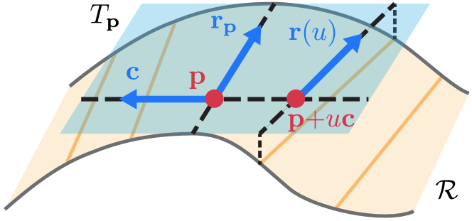
Figure 5. A schematic illustration of the local parameterization in Eq. (3), which is constructed by projecting the adjacent rulings of a point $\mathbf{p}$ onto its tangent plane $T_{\mathbf{p}}$.

On a triangle mesh, we consider each face as a tangent plane at the centroid of the face, and adopt the local model (6) as a discrete representation of the rulings on the face. Specifically, for a face $f$, let $\mathbf{v}_{f,1},\mathbf{v}_{f,2},\mathbf{v}_{f,3}\in\mathbb{R}^{3}$ be its three vertices according to a pre-defined orientation. We assign to the face centroid $\mathbf{o}_{f}$ a unit ruling direction $\mathbf{r}_{f}$, represented as a linear combination of two edge vectors $\mathbf{h}_{f,1}=\mathbf{v}_{f,2}-\mathbf{v}_{f,1}$ and $\mathbf{h}_{f,2}=\mathbf{v}_{f,3}-\mathbf{v}_{f,1}$ with scalar parameters $a_{f},b_{f}\in\mathbb{R}$:

(7) $$\mathbf{r}_{f}=(a_{f}\mathbf{h}_{f,1}+b_{f}\mathbf{h}_{f,2})/{\|a_{f}\mathbf{h}_{f,1}+b_{f}\mathbf{h}_{f,2}\|}.$$

By construction, $\mathbf{r}_{f}$ is orthogonal to the face normal $\mathbf{n}_{f}=\frac{\mathbf{h}_{f,1}\times\mathbf{h}_{f,2}}{\|\mathbf{h}_{f,1}\times\mathbf{h}_{f,2}\|}$. We also compute a unit vector

(8) $$\mathbf{c}_{f}=\mathbf{n}_{f}\times\mathbf{r}_{f}$$

that belongs to the tangent space and is orthogonal to $\mathbf{r}_{f}$. Then, applying Eq. (6) at $\mathbf{o}_{f}$, we obtain a local parameterization of $f$ that encodes the rulings on the face:

(9) $${\mathbf{q}}_{f}(u,v)=\mathbf{o}_{f}+u~\mathbf{c}_{f}+v(\mathbf{r}_{f}+u~\gamma_{f}~\mathbf{c}_{f}),$$

where $\gamma_{f}\in\mathbb{R}$ is a ruling variation parameter. Using Eq. (9), the ruling direction (without normalization) at any point $\mathbf{s}$ on the face can be computed as (see Appendix A):

(10) $$\overline{\mathbf{r}}_{f}({\mathbf{s}})=(1+\gamma_{f}x_{\mathbf{s}})\mathbf{r}_{f}+\gamma_{f}y_{\mathbf{s}}\mathbf{c}_{f},\quad\text{if}~1+\gamma_{f}x_{\mathbf{s}}\neq 0.$$

Here $x_{\mathbf{s}}=(\mathbf{s}-\mathbf{o}_{f})\cdot\mathbf{r}_{f}$ and $y_{\mathbf{s}}=(\mathbf{s}-\mathbf{o}_{f})\cdot\mathbf{c}_{f}$ are local coordinates of $\mathbf{s}$ with respect to the origin $\mathbf{o}_{f}$ and axes ($\mathbf{r}_{f}$,$\mathbf{c}_{f}$). Moreover, it can be shown that the condition $1+\gamma_{f}x_{\mathbf{s}}\neq 0$ is satisfied on the whole face if the following condition is satisfied at the three vertices (see Appendix B for a proof):

(11) $$1+\gamma_{f}~x_{\mathbf{v}_{f,i}}>0,\quad\text{for}~i=1,2,3.$$

Thus, we enforce (11) as a hard constraint for the parameter $\gamma_{f}$.

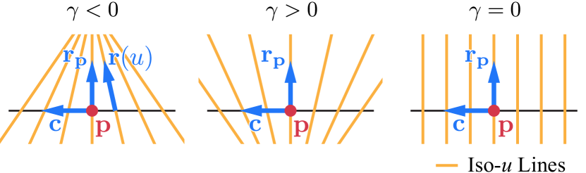
Figure 6. In our local model (6) of a ruled surface, the iso-$u$ lines are straight line segments that approximate the rulings around the point $\mathbf{p}$, whereas the parameter $\gamma$ captures the local variation of the rulings.

To summarize, on each mesh face we represent the ruling direction field using Eq. (10), where the parameters $(a_{f},b_{f})$ and $\gamma_{f}$ encode the direction at the centroid and the local variation of directions respectively, and $\gamma_{f}$ is subject to the constraint (11). By construction, an integral curve of the vector field (10) within the face is a straight line segment. Thus, tracing the vector field across the mesh surface results in a polyline approximating a true ruling on the underlying smooth surface. With properly chosen parameters, this polyline can provide a more accurate approximation than tracing along a piecewise constant vector field, as shown in Fig. 4.

3.1.2. Optimization formulation

Our optimization is based on the following key observation: on a ruled surface, the ruling direction at each point is an asymptotic direction with zero normal curvature (Flöry et al., 2013); moreover, being a straight line that lies on the surface, it must also be a geodesic curve. In the following, we propose a formulation that induces these properties on the optimized surface while enforcing its closeness to the target shape.

Geodesic condition

With the above observation, we require the integral curves of our ruling direction field to be as close to discrete geodesics as possible. We adopt the following conditions from (Polthier and Schmies, 1998) for discrete geodesics on triangle meshes:

1. Inside each face, a discrete geodesic is a straight line segment.

2. For a discrete geodesic crossing the interior of a mesh edge, if the two adjacent faces of this edge are unfolded around the edge into a common plane, then the geodesic segments on the two faces are unfolded into a common line segment (see inset figure).

Our ruling direction field already satisfies Condition (a) by construction. For Condition (b), let $f_{i},f_{j}$ be two triangle faces sharing a common edge $e_{ij}$ with end points $(\mathbf{v}_{1}^{i,j},\mathbf{v}_{2}^{i,j})$, and let $\mathbf{v}_{3}^{i,j},\mathbf{v}_{4}^{i,j}$ be the remaining vertices from $f_{i}$ and $f_{j}$ respectively. We choose

(12) $$\mathbf{B}_{i,j}^{i}=[\mathbf{e}_{ij},\mathbf{e}_{ij}\times\mathbf{n}_{i}],\qquad\mathbf{B}_{i,j}^{j}=[\mathbf{e}_{ij},\mathbf{e}_{ij}\times\mathbf{n}_{j}]$$

as the local bases for the two faces, where $\mathbf{e}_{ij}=\frac{\mathbf{v}_{2}^{i,j}-\mathbf{v}_{1}^{i,j}}{\|\mathbf{v}_{2}^{i,j}-\mathbf{v}_{1}^{i,j}\|}$ is the unit edge vector, and $\mathbf{n}_{i},\mathbf{n}_{j}$ are the unit face normals of $f_{i}$ and $f_{j}$ respectively. $\mathbf{B}_{i,j}^{i}$ and $\mathbf{B}_{i,j}^{j}$ will align after the two faces are unfolded into a common plane. If an integral curve interests with $e_{ij}$ at an interior point $\mathbf{q}$, then its two segments on $f_{i}$ and $f_{j}$ will have unit directions

$$\mathbf{s}_{i}=\overline{\mathbf{r}}_{f_{i}}(\mathbf{q})/\|\overline{\mathbf{r}}_{f_{i}}(\mathbf{q})\|,\qquad\mathbf{s}_{j}=\overline{\mathbf{r}}_{f_{j}}(\mathbf{q})/\|\overline{\mathbf{r}}_{f_{j}}(\mathbf{q})\|$$

respectively according to Eq. (10). We use the following function to compare the local coordinates of $\mathbf{s}_{i}$ and $\mathbf{s}_{j}$ in the bases $\mathbf{B}_{i,j}^{i}$ and $\mathbf{B}_{i,j}^{j}$ respectively:

$$E_{\text{geod}}^{i,j}(\mathbf{q})=\left\|(\mathbf{B}_{i,j}^{i})^{T}\mathbf{s}_{i}-(\mathbf{B}_{i,j}^{j})^{T}\mathbf{s}_{j}\right\|^{2}.$$

Note that the above measure can be seen as a discrete geodesic curvature of the integral curve at $\mathbf{q}$ that indicates its violation of Condition (b). To enforce Condition (b) along the whole edge $e_{ij}$, we evenly sample $k$ points in the interior of $e_{ij}$, and define an error term for $e_{ij}$ as

$$E_{\text{geod}}(e_{ij})=\sum\nolimits_{\mathbf{q}\in\mathcal{S}_{ij}}E_{\text{geod}}^{i,j}(\mathbf{q}),$$

where $\mathcal{S}_{ij}$ denotes the set of sample points.

Curvature condition

As the ruling direction is also an asymptotic direction, it induces conditions on the local curvature of the underlying surface. Let $\mathbf{b}_{1},\mathbf{b}_{2}$ be the principal directions at a point $\mathbf{p}$ on a smooth surface, and $\kappa_{1},\kappa_{2}$ be the corresponding principal curvatures. Then, the normal curvature along a tangent direction $\mathbf{d}$ at $\mathbf{p}$ can be computed as (do Carmo, 1976):

$$\kappa_{n}{}(\mathbf{d})=\kappa_{1}\cos^{2}\theta+\kappa_{2}\sin^{2}\theta,$$

where $\theta$ is the angle between $\mathbf{b}_{1}$ and $\mathbf{d}$. If $\mathbf{d}$ is an asymptotic direction (i.e., $\kappa_{n}{}(\mathbf{d})=0$), then $\kappa_{1}$ and $\kappa_{2}$ must satisfy

(13) $$\kappa_{1}=\mu\sin^{2}\theta,\quad\kappa_{2}=-\mu\cos^{2}\theta,$$

for a certain $\mu\in\mathbb{R}$. We use this condition to parameterize the principal curvatures and principal directions on mesh faces. Specifically,

on each face $f$, we introduce a variable $\theta_{f}\in\mathbb{R}$ for the signed angle from the ruling direction $\mathbf{r}_{f}$ (defined in Eq. (7)) to the principal direction $\mathbf{b}_{f,1}$ at the centroid $\mathbf{o}_{f}$ (see inset figure). Then the principal directions $\mathbf{b}_{f,1},\mathbf{b}_{f,2}$ at $\mathbf{o}_{f}$ can be represented as

(14) $$\mathbf{b}_{f,1}=\cos\theta_{f}~\mathbf{r}_{f}+\sin\theta_{f}~\mathbf{c}_{f},\quad\mathbf{b}_{f,2}=-\sin\theta_{f}~\mathbf{r}_{f}+\cos\theta_{f}~\mathbf{c}_{f},$$

where $\mathbf{c}_{f}$ is defined in Eq. (8). We also introduce a variable $\mu_{f}\in\mathbb{R}$ and apply Eq. (13) to represent the principal curvatures on at $\mathbf{o}_{f}$ as

(15) $$\kappa_{f,1}=\mu_{f}\sin^{2}\theta_{f},\quad\kappa_{f,2}=-\mu_{f}\cos^{2}\theta_{f}.$$

Using $\mathbf{B}_{f}=[\mathbf{b}_{f,1},\mathbf{b}_{f,2}]\in\mathbb{R}^{3\times 2}$ as the local bases for the tangent space $T_{\mathbf{o}_{f}}$ of $\mathbf{o}_{f}$, the second fundamental tensor $\mathbf{M}_{f}:T_{\mathbf{o}_{f}}\mapsto T_{\mathbf{o}_{f}}$ at $\mathbf{o}_{f}$ has the form

$$\mathbf{M}_{f}=\begin{bmatrix}\kappa_{f,1}&0\\ 0&\kappa_{f,2}\end{bmatrix}.$$

$\mathbf{M}_{f}$ maps each tangent vector $\mathbf{t}\in T_{\mathbf{o}_{f}}$ to the variation of normal along $\mathbf{t}$, and should be consistent with surface normals around $f$. Thus, for a face $f^{\prime}$ that shares a common edge with $f$, we use the following term to measure the consistency between $\mathbf{M}_{f}$ and the normals at $f$ and $f^{\prime}$:

$$E({f},f^{\prime})=\|\mathbf{M}_{f}\mathbf{B}_{f}^{T}\mathbf{g}_{f,f^{\prime}}-\mathbf{B}_{f}^{T}(\mathbf{n}_{f^{\prime}}-\mathbf{n}_{f})\|^{2}\mathbin{/}\|\mathbf{g}_{f,f^{\prime}}\|^{2}.$$

Here $\mathbf{n}_{f},\mathbf{n}_{f^{\prime}}\in\mathbb{R}^{3}$ are the unit face normals of $f$ and $f^{\prime}$, respectively. $\mathbf{g}_{f,f^{\prime}}=\overline{\mathbf{o}}_{f^{\prime}}-\mathbf{o}_{f}$ is a tangent vector in $T_{\mathbf{o}_{f}}$ indicating the geodesic displacement between the centroids of $f$ and $f^{\prime}$, where $\overline{\mathbf{o}}_{f^{\prime}}$ is the centroid of $f^{\prime}$ after it is unfolded into the same plane as $f$ around their common edge (see inset figure). Then, for each interior edge $e_{ij}$ shared by two faces $f_{i}$ and $f_{j}$, we introduce a term to enforce consistency between the curvature information on the two faces:

$$E_{\text{curv}}(e_{ij})=E({f_{i}},f_{j})+E({f_{j}},f_{i}).$$

Group-sparsity optimization

For a mesh edge $e_{ij}$ inside a ruled surface patch, the terms $E_{\text{geod}}(e_{ij})$ and $E_{\text{curv}}(e_{ij})$ should both have small values. On the other hand, for an edge on the boundary between two patches, at least one of the terms may have a large value due to the discontinuity of ruling directions and/or curvature information. Therefore, if we simply minimize the sum of these terms over all edges, then such least-squares optimization will penalize large term values everywhere and may prevent a desirable piecewise ruled shape from emerging. To address this issue, we adopt a group-sparsity formulation (Bach et al., 2012): for each interior mesh edge $e_{ij}$, we use the Welsch’s function (Holland and Welsch, 1977) as a robust norm and apply it to the combined error

(16) $$E_{\text{comb}}(e_{ij})=E_{\text{geod}}(e_{ij})+E_{\text{curv}}(e_{ij}),$$

resulting in the following sparsity term for the edge errors:

(17) $$E_{\text{sparse}}=\sum\nolimits_{e_{ij}\in\mathcal{E}_{I}}\psi_{\nu}\left(\sqrt{E_{\text{comb}}(e_{ij})}\right),$$

where $\psi_{\nu}$ is the Welsch’s function defined as

$$\psi_{\nu}(x)=1-\exp\left(-\frac{x^{2}}{2\nu^{2}}\right),$$

and $\nu>0$ is a user-specified parameter. $\psi_{\nu}(\cdot)$ is bounded from above and insensitive to large $x$ values due to its small derivatives at such values. Meanwhile, it effectively penalizes the magnitude of $x$ when $x$ is closer to zero. Thus $E_{\text{sparse}}$ can help reduce the error value $E_{\text{inte}}$ for edges in the interior of a ruled surface patch while allowing for edges with large errors on the boundaries between patches, facilitating our optimization towards a piecewise ruled shape.

Shape closeness

To align with the target shape, we introduce a closeness term that penalizes the deviation from each mesh vertex position $\mathbf{v}$ to the target:

(18) $$E_{\text{close}}(\mathbf{v})=\|\mathbf{v}-P(\mathbf{v})\|^{2},$$

where $P(\cdot)$ denotes the closest-point projection onto the target surface (for interior vertices) or its boundary (for boundary vertices).

Barrier Terms

We also introduce a barrier term to ensure the variation parameter $\gamma_{f}$ on each face $f$ satisfies the condition (11):

(19) $$E_{\text{barr}}(f)=\sum\nolimits_{i=1}^{3}({1+\gamma_{f}~x_{\mathbf{v}_{f,i}}})^{-2}.$$

$E_{\text{barr}}(f)$ will approach infinity when $1+\gamma_{f}~x_{\mathbf{v}_{f,i}}$ approaches zero. Thus, if we start from variable values that satisfy condition (11) and employ a numerical solver that enforces monotonic decrease of the target function, the term will prevent $\gamma_{f}$ from reaching the boundary of its feasible set and ensure condition (11) remains satisfied.

Regularization

We use regularizer terms to ensure smooth deformation and avoid degenerate triangles. For smoothness, we use a Laplacian term for the displacement of each vertex ${v}$

(20) $$E_{\text{lap}}(v)=\left\|(\mathbf{v}-\mathbf{v}^{(0)})-\frac{1}{|\mathcal{N}(v)|}\sum\nolimits_{v_{j}\in\mathcal{N}(v)}(\mathbf{v}_{j}-\mathbf{v}_{j}^{(0)})\right\|^{2},$$

where $\mathcal{N}(v)$ denotes the set of adjacent vertices (for an interior vertex) or the set of adjacent boundary vertices (for a boundary vertex), and $\mathbf{v}^{(0)}$ denotes the vertex position on the initial mesh.

To avoid degenerate triangles, we use the following term on each edge $e$ to prevent excessive changes in edge length:

(21) $$E_{\text{len}}(e)=({\|\mathbf{h}_{e}\|-\|\mathbf{h}_{e}^{(0)}\|})^{2}\mathbin{/}\|\mathbf{h}_{e}^{(0)}\|^{2},$$

where $\mathbf{h}_{e}$ and $\mathbf{h}_{e}^{(0)}$ are the edge vector of $e$ in the current mesh and the initial mesh, respectively.

Overall Formulation

Combining the terms presented above, we obtain the target function for our optimization:

(22) $$E= E_{\text{sparse}}+w_{1}\sum\nolimits_{v\in\mathcal{V}}E_{\text{close}}(v)+w_{2}\sum\nolimits_{f\in\mathcal{F}}E_{\text{barr}}(f)$$

$$+w_{3}\sum\nolimits_{v\in\mathcal{V}}E_{\text{lap}}(v)+w_{4}\sum\nolimits_{e\in\mathcal{E}}E_{\text{len}}(e),$$

where $\mathcal{V},\mathcal{E},\mathcal{F}$ denote the set of mesh vertices, mesh edges, and mesh faces respectively, $\mathcal{E}_{B}$ denotes the set of mesh boundary edges, $f_{e}$ denotes the only face adjacent to a mesh boundary edge $e$, and $w_{1},w_{3},w_{4},w_{2}$ are user-specified weights. The variables include all the mesh vertex positions, the parameters $\{(a_{f},b_{f},\gamma_{f})\}$ that represent the ruling direction field on each face, and the parameters $\{(\mu_{f},\theta_{f})\}$ that encode the local curvature information on each face.

We solve this problem numerically with an L-BFGS solver, using automatic differentiation to evaluate the gradient. To improve efficiency, the values and gradients of different target function terms are computed in parallel. It is also worth noting that the parameter $\nu$ in the Welsch’s function controls its robustness: With a $\nu$ closer to zero, the function is less sensitive to large error values, which would benefit the emergence of patch boundaries; however, if we use a very small value of $\nu$ during the whole process, $E_{\text{sparse}}$ would have small gradients on most surface areas and may fail to steer the mesh toward a desirable shape. Therefore, following existing methods that use the Welsch’s function as a robust norm (Zhang et al., 2022), we start with a large value $\nu_{\max}$ for $\nu$ and gradually decrease it to a minimum value $\nu_{\min}$ during optimization.

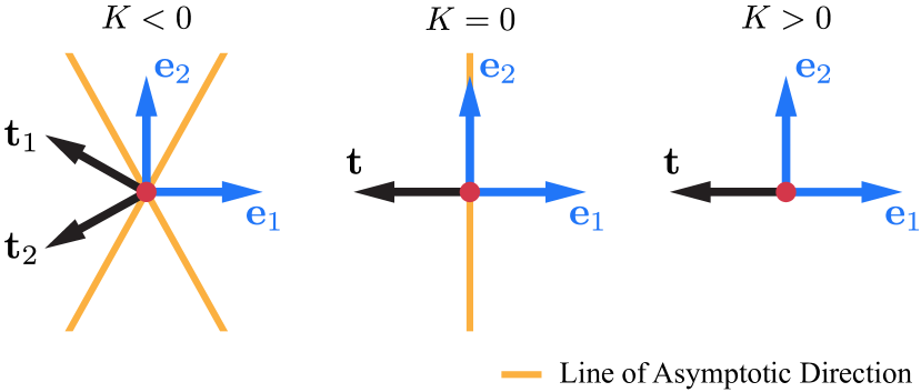
Figure 7. The definition of vector $\mathbf{t}$ used in Eq. (24) depending on the sign of the Gaussian curvature $K$. Here, $\mathbf{e}_{1}$ and $\mathbf{e}_{2}$ are principal directions, with their corresponding principal curvatures $\kappa_{1}$ and $\kappa_{2}$ satisfying $|\kappa_{1}|\geq|\kappa_{2}|$. With a negative Gaussian curvature, there are two vectors $\mathbf{t}_{1}$ and $\mathbf{t}_{2}$ orthogonal to the two lines of asymptotic direction, respectively. Otherwise, there is a single $\mathbf{t}$ parallel with $\mathbf{e}_{1}$.

3.1.3. Vector field initialization

Since our optimization problem is nonconvex, a proper initialization of the ruling direction field is necessary for the solver to produce desirable results. To this end, we initialize all ruling variation variable $\{\gamma_{f}\}$ to zero, and construct the initial ruling directions $\{\mathbf{r}_{f}\}$ at the face centroids as a smooth vector field. In (Flöry et al., 2013), it is suggested that the initial ruling directions should align with the asymptotic directions across the surface. However, this is ineffective for surface regions of positive Gaussian curvature, as there is no asymptotic direction there. Moreover, at a point of negative Gaussian curvature, there are more one asymptotic directions, and we need to choose one of them in a globally consistent way to ensure the overall smoothness of the resulting direction field. To address these challenges, we first generalize the condition in (Flöry et al., 2013): On each mesh face, we require the initial ruling direction to align with a tangent direction with the smallest magnitude of normal curvature. This is based on the following observation: At a point $\mathbf{p}$ on a surface, the normal curvature along a tangent direction $\mathbf{t}$ is the extrinsic curvature of the geodesic curve that passes through the point $\mathbf{p}$ along the direction $\mathbf{t}$; therefore, among all geodesic curves passing through $\mathbf{p}$, the one along the tangent direction with the minimum amount of normal curvature has the smallest local deviation from a straight line passing through $\mathbf{p}$ along the same tangent direction, making it suitable for our initialization. It is worth noting that at a point with non-positive Gaussian curvature, our condition is equivalent to the one proposed in (Flöry et al., 2013), since the normal curvature attains the minimum magnitude of zero along the asymptotic directions. Therefore, our condition is a generalization of the one in (Flöry et al., 2013). Meanwhile, at a point with positive Gaussian curvature, our condition requires the initial direction to align with a principal direction with the smallest magnitude of principal curvature. To define the target directions, we use the method of (Rusinkiewicz, 2004) to determine the principal directions and principal curvatures on each face.

To determine a smooth vector field $\{\mathbf{r}_{f}\}$ that meets the alignment condition mentioned above, we first construct a local orthonormal bases $\mathbf{D}_{f}\in\mathbb{R}^{3\times 2}$ for each face $f$ and represent $\mathbf{r}_{f}$ as $\mathbf{r}_{f}=\mathbf{D}_{f}\mathbf{y}_{f}$ with local coordinates $\mathbf{y}_{f}\in\mathbb{R}^{2}$. Then we solve an optimization problem for $\{\mathbf{y}_{f}\}$:

(23) $$\min_{\{\mathbf{y}_{f}\}}~E_{\text{smo}}+\mu_{1}E_{\text{unit}}+~\mu_{2}\sum_{f\in\mathcal{F}_{\textrm{np}}}E_{\text{align}}(\mathbf{y}_{f})~+\mu_{3}\sum_{f^{\prime}\in\mathcal{F}_{\textrm{p}}}E_{\text{align}}(\mathbf{y}_{f^{\prime}}),$$

where $\mu_{1}$, $\mu_{2}$ and $\mu_{3}$ are user-specified weights. Here, the term

(24) $$E_{\text{align}}(\mathbf{y}_{f})=\min_{\mathbf{t}\in\mathcal{A}_{f}}\|\mathbf{y}_{f}\cdot\mathbf{t}\|^{2}$$

measures the alignment between $\mathbf{y}_{f}$ and its target directions defined above, where $\mathcal{A}_{f}$ is a set of unit tangent vectors orthogonal to target direction and represented with local coordinates with respect to $\mathbf{D}_{f}$, and $\mathcal{F}_{\textrm{np}}$, $\mathcal{F}_{\textrm{p}}$ denote the set of faces with non-positive Gaussian curvature and positive Gaussian curvature, respectively. On a face with non-negative Gaussian curvature, $\mathcal{A}_{f}$ contains only one vector along the principal direction with the largest magnitude of principal curvature. On a face with negative Gaussian curvature, $\mathcal{A}_{f}$ contains two vectors orthogonal to the two lines of asymptotic direction, respectively (see Fig. 7).

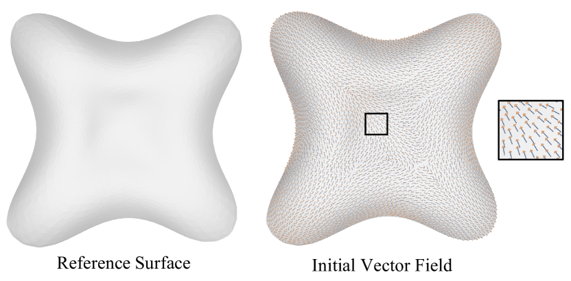
Figure 8. An initial vector field computed using the method in Sec. 3.1.3.

Additionally, the term $E_{\text{smo}}$ measures the smoothness of the vector field by comparing its values on each pair of adjacent faces $f_{i},f_{j}$ after unfolding them into a common plane around their shared edge:

$$E_{\text{smo}}=\sum_{e_{ij}\in\mathcal{E}_{I}}\|(\mathbf{B}_{i,j}^{i})^{T}\mathbf{D}_{f_{i}}\mathbf{y}_{f_{i}}-(\mathbf{B}_{i,j}^{j})^{T}\mathbf{D}_{f_{j}}\mathbf{y}_{f_{j}}\|^{2},$$

where $\mathbf{B}_{i,j}^{i},\mathbf{B}_{i,j}^{j}$ are local bases defined in Eq. (12). Lastly, the term

$$E_{\text{unit}}=\sum_{f\in\mathcal{F}}\left\|\mathbf{y}_{f}-\frac{\mathbf{y}_{f}}{\|\mathbf{y}_{f}\|}\right\|^{2}$$

enforces a unit-length condition for the vectors $\{\mathbf{y}_{f}\}$ as well as $\{\mathbf{r}_{f}\}$. We solve the problem (23) using a majorization-minimization (MM) solver (Lange, 2016). Full details can be found in Appendix D.

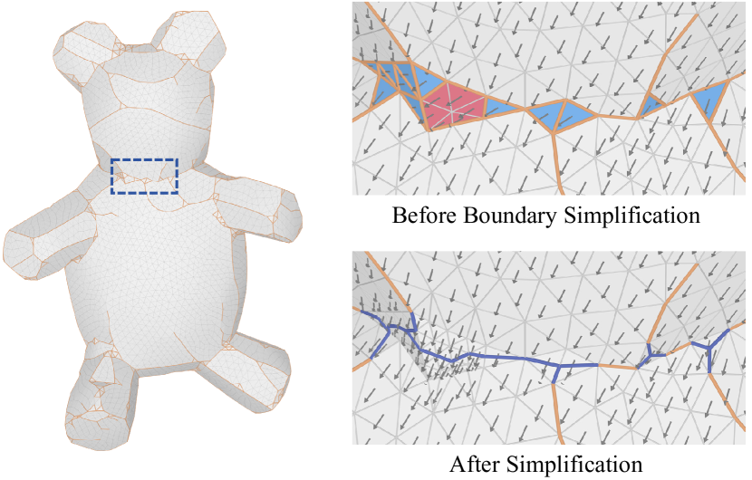
Figure 9. An example of boundary simplification when extracting the initial patch boundaries. Top right: we first extract candidate edges (shown in brown) for the patch boundary segments according to the optimized ruling direction field (shown in gray), as well as areas where we need to perform boundary simplification; the simplification areas include faces with at least two candidate edges (shown in blue) and small areas enclosed by candidates edges (shown in red). Bottom right: within each simplification area, we use graph cut to create simple boundary segments (shown in purple) connecting the candidate edges outside the area, and further optimize the ruling direction field inside the area according to target function (25).

3.2. Initial Piecewise Ruled Surface

After the joint optimization of the mesh shape and the ruling direction field, we use the optimization result to extract polyline boundaries between ruled surface patches and construct initial rulings that connect these boundaries. As candidates of boundary segments, we first extract a set $\mathcal{C}_{\text{B}}$ of edges whose combined error values $E_{\text{comb}}$ defined in Eq. (16) are larger than a threshold $\epsilon_{\text{edge}}$. The union of these candidate edges may have complicated topologies such as small loops (e.g., see Fig. 9), which are not suitable for our boundary representation. Therefore, we clean up the candidates and construct simple boundaries as follows. First, we identify a set $\mathcal{F}_{\text{B}}$ of faces that represent the regions that require boundary segment simplification. The set $\mathcal{F}_{\text{B}}$ includes all faces that contain at least two edges from $\mathcal{C}_{\text{B}}$. Furthermore, if some edges in $\mathcal{C}_{\text{B}}$ form a loop that encloses an area smaller than a threshold $\epsilon_{A}$, we add all the enclosed faces to $\mathcal{F}_{\text{B}}$ to avoid creating a very small patch. Candidate edges in $\mathcal{C}_{\text{B}}$ that do not belong to the faces in $\mathcal{F}_{\text{B}}$ are directly used as part of the boundary, while additional boundary segments are constructed on the faces in $\mathcal{F}_{\text{B}}$ using the following steps. First, we determine the connected components of $\mathcal{F}_{\text{B}}$ based on their dual-graph connectivity (i.e., each mesh face is a vertex in the dual graph, and two dual-graph vertices are connected if their corresponding faces in the primal mesh share a common edge) and construct patch boundary segments inside each component $\mathcal{S}$ according to candidate edges that are outside $\mathcal{S}$ but attached to its boundary vertices. In the following, we call such a vertex a split vertex. Our goal is to construct boundary segments that have simple shapes and connect these split vertices, in order to form continuous boundaries with simple topology (see Fig. 9 for an example). To this end, we consider two cases:

• If the component $\mathcal{S}$ is a single face, then we construct a set of patch boundary segments within the face according to the number of its split vertices. We consider four sub-cases (see Fig. 10):

  1. If there is no split vertex, we choose the longest edge of the face as the only patch boundary segment.

  2. If there is one split vertex, we choose the longest edge attached to this vertex.

  3. If there are two split vertices, we choose the edge between them.

  4. If there are three split vertices, we add a new vertex at the face centroid and connect it with the three face vertices to subdivide the face into three smaller faces, and then choose the edges between the three faces as the patch boundary segments.

  Figure 10. Construction of patch boundary segments on a connected component $\mathcal{S}$ with a single face, according to the number of its split vertices.

• If $\mathcal{S}$ contains more than one face, then we consider different cases according to the number of split vertices on the boundary of $\mathcal{S}$:

  1. If there are $N$ split vertices with $N\geq 2$, then they divide the boundary of $\mathcal{S}$ into $N$ segments. We perform a graph cut optimization to divide $\mathcal{S}$ into $N$ regions, so that each region is attached to one boundary segment of $\mathcal{S}$ (see Appendix E for details). In this way, the boundaries between the regions connect the split vertices, while the graph cut helps achieve their smile shapes. We then add the inter-region boundaries as the patch boundary segments.

  2. If there is only one split vertex $\mathbf{q}$, then we find a vertex $\mathbf{q}^{\ast}$ on the boundary $\mathcal{S}$ with the largest geodesic distance to $\mathbf{q}$, and add $\mathbf{q}^{\ast}$ as a virtual split vertex. Afterward, we have two split vertices, and we use the same procedure as Case (1) above to construct the patch boundary segments. In this way, the resulting segments align with the overall shape of $\mathcal{S}$.

  3. If there is no split vertex, then we find a pair of vertices $\mathbf{q}^{\ast}_{1}$ and $\mathbf{q}^{\ast}_{2}$ on the boundary of $\mathcal{S}$ with the largest value of geodesic distance among all such pairs. We then add $\mathbf{q}^{\ast}_{1}$, $\mathbf{q}^{\ast}_{2}$ as virtual split vertices, and apply the procedure in Case (1).

The polyline segments produced by the above procedure, together with the remaining candidate edges from $\mathcal{C}_{\text{B}}$ that are outside $\mathcal{F}_{\text{B}}$, form the full patch boundaries. It is worth noting that our approach may produce not only boundary loops that fully enclose the patches, but also isolated non-loop boundary segments. We allow such non-loop segments as they enable a better approximation of the target shape, such as in areas with positive Gaussian curvature surrounded by negative Gaussian curvature regions.

After the clean-up, we further optimize the ruling direction field on $\mathcal{S}$ by minimizing a target energy

(25) $$\sum_{e_{ij}\in\mathcal{E}_{\mathcal{S}}}E_{\text{geod}}(e_{ij}),$$

where $\mathcal{E}_{\mathcal{S}}$ is the set of mesh edges in $\mathcal{S}$ that are not on a patch boundary segment. Since the patch topology has been determined, this optimization specifically reduces the geodesic curvature of integral curves in the patch interior, which facilitates our construction of initial rulings.

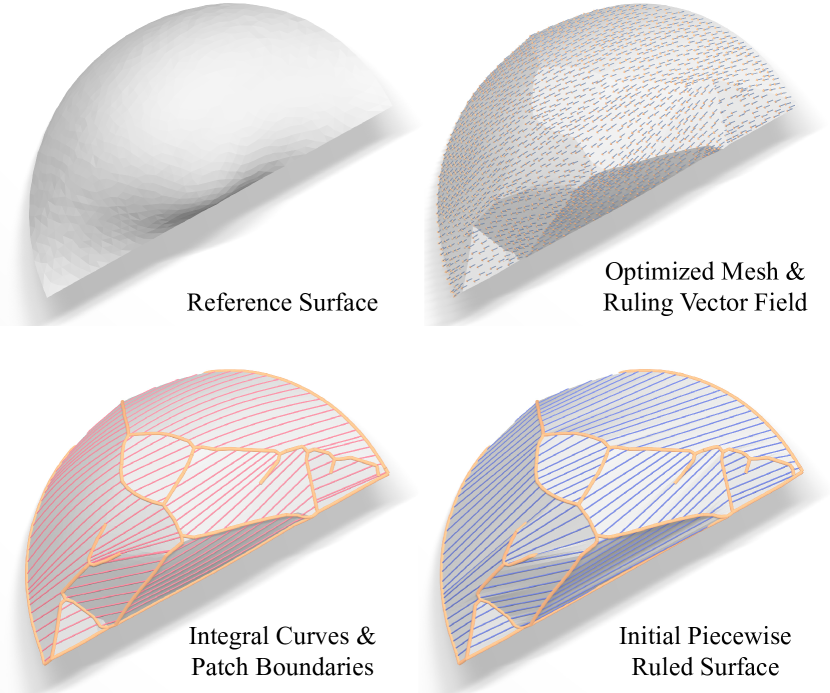
Figure 11. Construction of the initial piecewise ruled surface. Using the optimized mesh and ruling vector field (top right), we extract the initial patch boundary and trace along the vector field to derive integral curves (bottom left). Then we connect the two end points of each integral curve on the patch boundaries to derive the initial rulings (bottom right).

Finally, we start from sample points on the optimized mesh and trace along the ruling vector field, to produce a dense set of polyline integral curves whose endpoints lie on the patch boundaries. We then connect the two endpoints of each integral curve to derive the initial rulings (see Fig. 11 for an example).

3.3. Piecewise Ruled Surface Optimization

The initial rulings constructed in Section 3.2 already align roughly with the target shape. As the final step, we perform an optimization to further improve the alignment. To this end, we first replace the interior vertices of the patch boundary polylines with the ruling endpoints on the polyline. In this way, the vertices of the new boundary polylines control both the boundary shape and the positions and orientations of the rulings, facilitating our optimization formulation. We then optimize the vertex positions $\{\mathbf{b}_{i}\}$ of the boundary polylines, to align the piecewise ruled surface with the target shape while ensuring the smoothness of both the patches and their boundaries.

We enforce the surface alignment using the following target term that penalizes the distance to the target surface for both the patch boundaries and the rulings:

$$E_{\text{disp}}=\frac{\lambda_{1}}{M_{1}}\sum\nolimits_{\mathbf{s}\in\mathbf{S}_{\text{r}}}\alpha_{\mathbf{s}}E_{\text{close}}(\mathbf{s})+\frac{\lambda_{2}}{M_{2}}\sum\nolimits_{\mathbf{b}\in\mathbf{S}_{\text{b}}}\alpha_{\mathbf{b}}E_{\text{close}}(\mathbf{b}).$$

Here $E_{\text{close}}$ is defined in Eq. (18), and the sets $\mathbf{S}_{\text{r}}$ and $\mathbf{S}_{\text{b}}$ contain the patch boundary polyline vertices and uniform sample points on the rulings, respectively. Each sample point on a ruling is represented as a convex combination of its two endpoints with fixed weights. $\alpha_{\mathbf{p}}$ is an constant weight that equals the squared mean distance from $\mathbf{p}$ to its $k$-nearest neighbors in the set $\mathbf{S}_{\text{r}}\cup\mathbf{S}_{\text{b}}$, computed using their initial positions. $M_{1}=\sum_{\mathbf{s}\in\mathbf{S}_{\text{r}}}\alpha_{\mathbf{s}}$ and $M_{2}=\sum_{\mathbf{b}\in\mathbf{S}_{\text{b}}}\alpha_{\mathbf{b}}$ are normalization factors. And $\lambda_{1}$, $\lambda_{2}$ are user-specified weights.

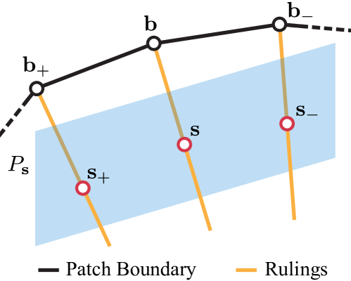
Figure 12. Definition of the points $\mathbf{b}$, $\mathbf{b}_{+}$, $\mathbf{b}_{-}$ and $\mathbf{s}$, $\mathbf{s}_{+}$, $\mathbf{s}_{-}$ for the curvature functions in Eq. (26) and Eq. (27), respectively.

Additionally, we enforce the smoothness of patch shapes by penalizing their curvature. Specifically, for each sample point $\mathbf{s}$ on a ruling, we construct a plane ${P}_{\mathbf{s}}$ that contains $\mathbf{s}$ and is orthogonal to the ruling, and intersect ${P}_{\mathbf{s}}$ with the two adjacent rulings to obtain points $\mathbf{s}_{+}$ and $\mathbf{s}_{-}$ (see Fig. 12). Then we use the function

(26) $$K_{\text{r}}(\mathbf{s})=\left\|\frac{({\mathbf{s}_{+}-\mathbf{s}}){/}{\|\mathbf{s}_{+}-\mathbf{s}\|}-(\mathbf{s}-\mathbf{s}_{-}){/}{\|\mathbf{s}-\mathbf{s}_{-}\|}}{({\|\mathbf{s}_{+}-\mathbf{s}\|+\|\mathbf{s}-\mathbf{s}_{-}\|}){/}{2}}\right\|$$

to measure the magnitude of the ruled surface’s discrete normal curvature at $\mathbf{s}$ along the direction orthogonal to the ruling. Based on this function, we introduce a surface smoothness term:

$$E_{\text{rul}}=\frac{1}{M_{3}}\sum\nolimits_{\mathbf{s}\in\mathbf{S}_{\text{r}}}\beta_{\mathbf{s}}[K_{\text{r}}(\mathbf{s})]^{2},$$

where $\beta_{\mathbf{s}}$ is an area weight equal to the initial squared mean distance from ${\mathbf{s}}$ to its two nearest sample point on the same ruling and the closest sample point on each adjacent ruling, and $M_{3}=\sum_{\mathbf{s}\in\mathbf{S}_{\text{r}}}\beta_{\mathbf{s}}$.

Moreover, to enforce the smoothness of each patch boundary polyline, we evaluate the magnitude of its discrete curvature at each interior vertex $\mathbf{b}$ via

(27) $$K_{\text{b}}(\mathbf{b})=\left\|\frac{({\mathbf{b}_{+}-\mathbf{b}}){/}{\|\mathbf{b}_{+}-\mathbf{b}\|}-({\mathbf{b}-\mathbf{b}_{-}}){/}{\|\mathbf{b}-\mathbf{b}_{-}\|}}{(\|\mathbf{b}_{+}-\mathbf{b}\|+\|\mathbf{b}-\mathbf{b}_{-}\|){/}2}\right\|,$$

where $\mathbf{b}_{+}$ and $\mathbf{b}_{-}$ are the two adjacent vertices for $\mathbf{b}$ on the polyline (see Fig. 12). Then we introduce a boundary smoothness term:

$$E_{\text{bdr}}=\frac{1}{M_{4}}\sum\nolimits_{\mathbf{b}\in\mathbf{S}_{\text{b}}}\eta_{\mathbf{b}}[K_{\text{b}}(\mathbf{b})]^{2},$$

where $\eta_{\mathbf{b}}$ is a constant weight equal to the average initial distance from $\mathbf{b}$ to $\mathbf{b}^{-}$ and $\mathbf{b}^{+}$.

Our overall formulation is written as

(28) $$\min~E_{\text{disp}}+\lambda_{3}E_{\text{rul}}+\lambda_{4}E_{\text{bdr}},$$

where $\lambda_{3}$ and $\lambda_{4}$ are user-specified weights. We use a variant of Powell’s Dogleg method (Byrd et al., 1988) to solve this non-linear least-squares problem.

After the optimization, we can add more rulings between existing ones if needed for an application. Since the rulings define a discrete correspondence between the boundary polylines via their endpoints, a simple approach is to interpolate the correspondence using arc-length parameterization of the boundary polyline segments between the endpoints of two adjacent rulings, and then connect the interpolated corresponding points to form new rulings. Alternatively, if higher-order smoothness is required, we could convert the boundary polylines into smooth curves using cubic spline interpolation of the polyline vertices, and connect point pairs with corresponding parameters to create new rulings. In our experiments, we do not find a noticeable difference between the two approaches since the rulings are already dense before refinement.

4. Results

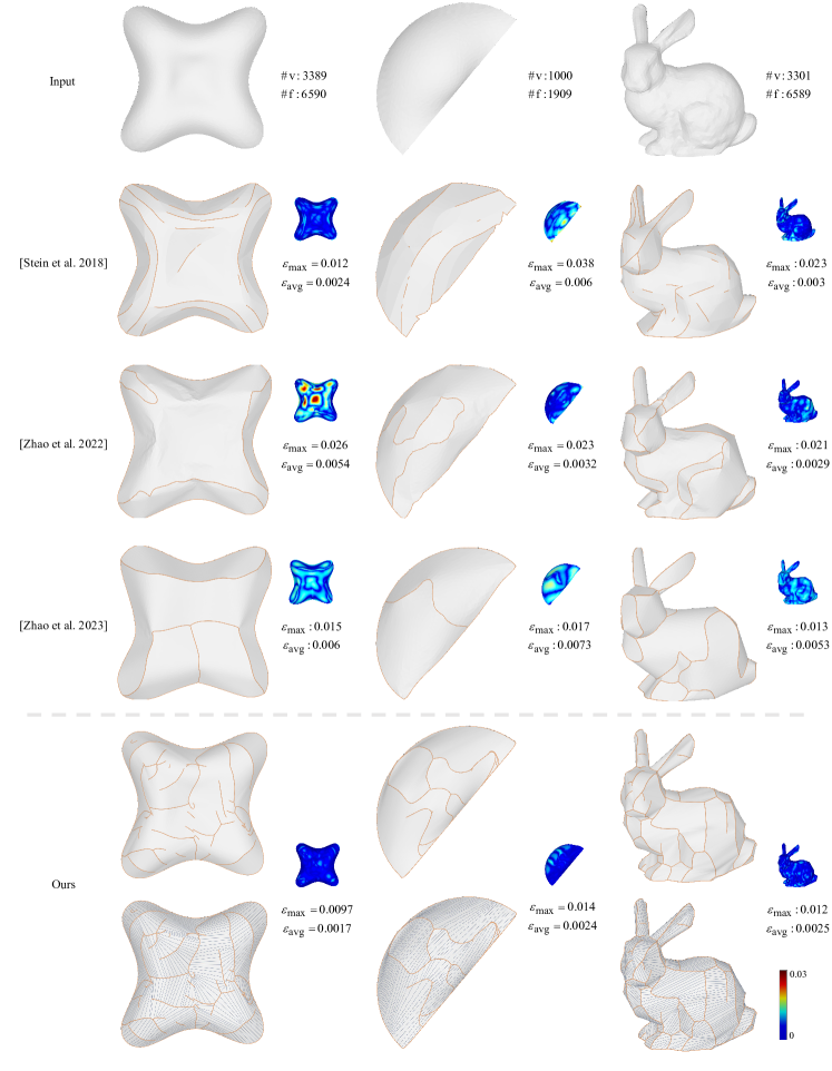
Figure 13. Comparison with (Stein et al., 2018), (Zhao et al., 2022) and (Zhao et al., 2023). The color coding shows the distance from the reference surface, normalized by the reference surface’s bounding box diagonal length.

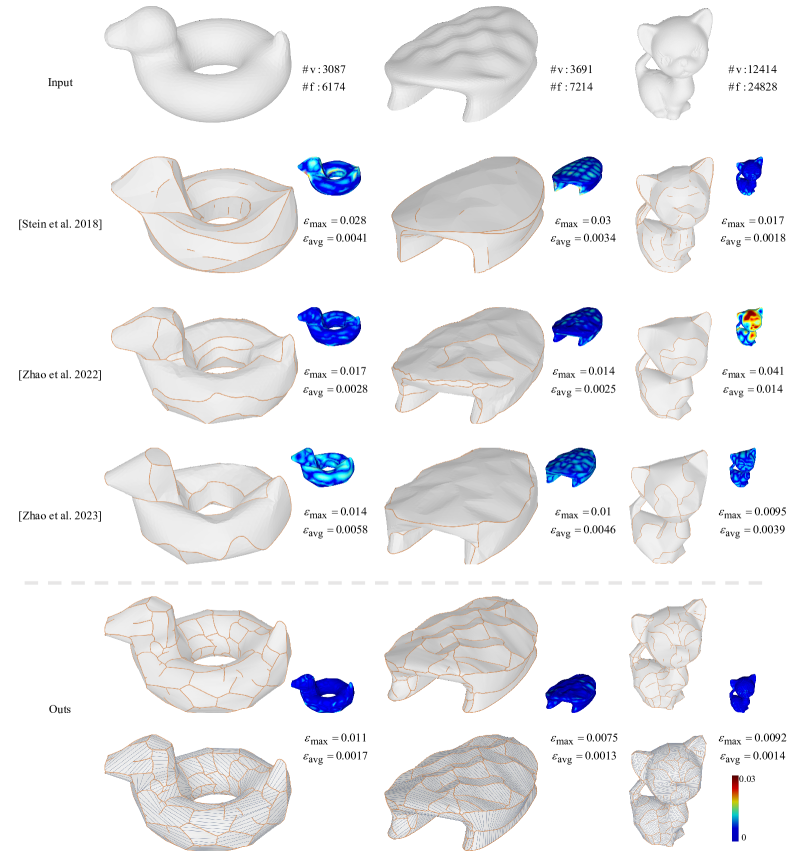
Figure 14. Comparison with (Stein et al., 2018), (Zhao et al., 2022) and (Zhao et al., 2023). The color coding shows the distance from the reference surface, normalized by the reference surface’s bounding box diagonal length.

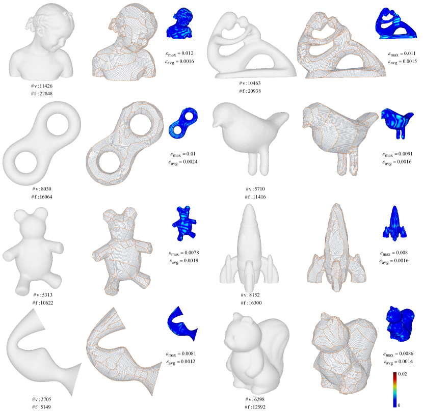
Figure 15. More results using our methods on various reference surfaces.

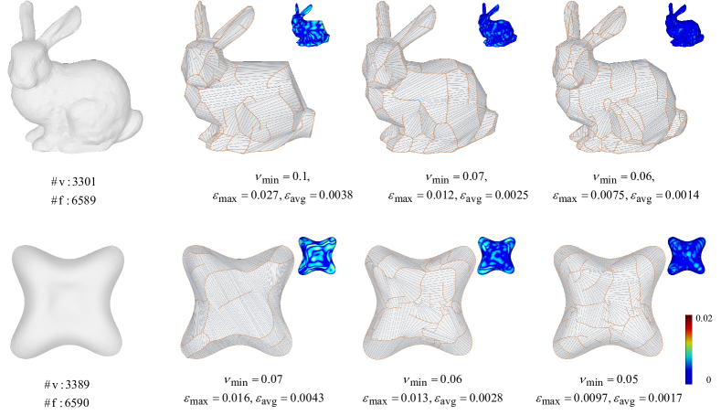
Figure 16. We can control the complexity of patch layout using the parameter $\nu_{\min}$ for the Welsch’s function in our optimization.

We implement our method in C++, using the Eigen library (Guennebaud et al., 2010) for linear algebra operations and OpenMP for parallelization. We use the L-BFGS solver from LBFGSpp  for the problem (22), and the Dogleg method from Ceres (Agarwal et al., 2023) for the problem (28). The parameter setting of our method is provided in Appendix C. All experiments are run on a PC with a 10-core Intel Core i9-10900 CPU at 2.8GHz and 32GB of RAM.

Comparison with other methods

We evaluate our method by testing it on a diverse set of freeform surfaces represented as triangle meshes, including both closed surfaces of non-zero genus and open surfaces with boundary. We compare our method against state-of-the-art methods for piecewise approximation of freeform mesh surfaces. As no existing piecewise ruled surface approximation method works on mesh surfaces as far as we are aware, we instead compare with three recent methods from (Stein et al., 2018), (Zhao et al., 2022) and (Zhao et al., 2023) that produce piecewise developable approximation. For each method, we use the open-source implementation^,, released by the authors in our comparison. To compare the performance between different methods, we evaluate each result using the average distance $\epsilon_{\textrm{avg}}$ and maximum distance $\epsilon_{\max}$ from sample points on the result surface to the original reference surface, normalized by the bonding box diagonal length of the reference surface. For our method, the sample points are the patch boundary vertices as well as uniform sample points from the rulings. For the other methods, the sample points are the vertices of the result surface mesh. The three methods for comparison are run using their default parameters provided in their open-source implementations.

Fig. 13 and Fig. 14 compare results for different methods on the same set of reference surfaces. To help visualize the patch layout of the piecewise developable results, we use the brown color to display the patch boundaries for (Zhao et al., 2022) and (Zhao et al., 2023) as indicated by their algorithm output, as well as mesh edges on the result of (Stein et al., 2018) where the dihedral angle is larger than 20 degrees. For each result, we include its error metric values $\epsilon_{\textrm{avg}}$, $\epsilon_{\max}$, and also use color coding to visualize its deviation from the reference surface. From the metric data and the visualization, we can see that our method achieves the lowest average error among all methods in all examples, and either the lowest or second-lowest maximum error in all examples. We also note that on models with large areas of negative Gaussian curvature (e.g., the top part of the ‘airport’ model in the middle column of Fig. 14), our method has an even stronger advantage in approximation error compared to the other three methods. This is not surprising since developable surfaces can only have zero Gaussian curvature while ruled surfaces allow for non-positive Gaussian curvature. Therefore, our piecewise ruled approximation provides more flexibility for accurate approximation in negative Gaussian curvature regions compared to piecewise developable surfaces. Fig. 15 shows more results of our method on reference surfaces with different shapes and topologies. In all examples, our maximum and average errors are no more than 1.5% and 0.25% of the reference shape’s bounding box diagonal length, respectively. Overall, the comparison and results verify the effectiveness of our method in approximating arbitrary freeform shapes with piecewise ruled surfaces with low approximation error.

Controllable boundary segments

The final value $\nu_{\min}$ of the parameter $\nu$ for the Welsch’s function in Eq. 17 affects the piecewise smoothness of the optimized ruling direction field. Decreasing $\nu_{\min}$ will enforce a stronger requirement of smoothness for the ruling vector field in the interior of a patch, which induces more edges with a large error value of $E_{\text{comb}}$ that indicates a patch boundary. As a result, the final piecewise ruled surface tends to have more patches while being closer to the target surface. On the other hand, increasing the value of $\nu_{\min}$ tends to produce a more simple patch layout with a larger deviation from the target surface. Thus the value of $\nu_{\min}$ can be used to control the complexity of the patch layout. Fig. 16 shows some examples of piecewise ruled surfaces resulting from different $\nu_{\min}$ for the same input target shapes.

Table 1. The computational time (in minutes) required by different methods for the models in Fig. 13 and Fig. 14, and the number of vertices and faces in the input models.

Model	Fig. 13			Fig. 14
	Lilium	Snail	Bunny	Bob	Airport	Kitten
#v	3389	1000	3301	3087	3691	12414
#f	6590	1909	6589	6174	7214	24828
(Stein et al., 2018)	11.5	2.3	12.3	10.7	3.5	55.7
(Zhao et al., 2022)	15.6	1.5	13.4	8.5	10.8	43.6
(Zhao et al., 2023)	6.8	3.1	6.0	4.4	4.9	36.2
Ours	5.3	1.2	5.4	4.3	2.7	24.8

Computational efficiency

Finally, Table. 1 compares the computational time required by each method for the results shown in Fig. 13 and Fig. 14. We can see that our method runs faster than all other methods on these examples. Further data for the results in Fig. 16 are provided in Appendix F. These data demonstrate the efficiency of our computational approach.

5. Limitations and Future Work

Currently, our method only considers geometric approximation of the target shape and does not enforce other application-specific conditions such as structural stability and accessibility for tools. Incorporating such conditions will be future work and will be beneficial for practical applications.

In addition, our piecewise construction always produces sharp edges at the patch boundaries. This is necessary for target surface areas with positive Gaussian curvature: as the interior of a ruled surface patch can only non-positive Gaussian curvature, the sharp edges are needed for ‘concentrating’ the positive Gaussian curvature of the target shape to the patch boundaries. However, for surface areas of non-positive Gaussian, it is possible to approximate them with ruled surface patches with continuous tangent planes but discontinuous ruling directions at their boundaries, producing a smooth appearance (Flöry et al., 2013). An interesting future work would be to improve our approach and adaptively enforce such tangent continuity conditions according to local curvature.

Appendix A Derivation of Eq. (10)

From Eq. (9), we have

$${\mathbf{q}}_{f}(u,v)=\mathbf{o}_{f}+v\mathbf{r}_{f}+u+\gamma_{f}uv\mathbf{c}_{f}+v(\mathbf{r}_{f}+u~\gamma_{f}~\mathbf{c}_{f}).$$

Therefore, if we $\mathbf{o}_{f}$ as the origin and $(\mathbf{r}_{f},\mathbf{c}_{f})$ as the axes of the local coordinate, then the local coordinates $(x_{\mathbf{s}},y_{\mathbf{s}})$ of a point with parameters $(u,v)$ satisfies

$$(v,u+\gamma_{f}uv)=(x_{\mathbf{s}},y_{\mathbf{s}})$$

$$\Rightarrow~ v=x_{\mathbf{s}},~u+\gamma_{f}uv=y_{\mathbf{s}}$$

$$\Rightarrow~ u+\gamma_{f}ux_{\mathbf{s}}=y_{\mathbf{s}}$$

$$\Rightarrow~ u=\frac{y_{\mathbf{s}}}{1+\gamma_{f}x_{\mathbf{s}}}$$

For the value $\frac{y_{\mathbf{s}}}{1+\gamma_{f}x_{\mathbf{s}}}$ to be well-defined, we must have $1+\gamma_{f}x_{\mathbf{s}}\neq 0$. Then, using Eqs. (4) and (5), the ruling direction at $\mathbf{s}$ has the form

$$\mathbf{r}_{f}+u\gamma_{f}\mathbf{c}_{f}=\mathbf{r}_{f}+\frac{y_{\mathbf{s}}}{1+\gamma_{f}x_{\mathbf{s}}}\gamma_{f}\mathbf{c}_{f}.$$

Scaling this vector by $1+\gamma_{f}x_{\mathbf{s}}$ (which changes its length but does not change the direction as $1+\gamma_{f}x_{\mathbf{s}}\neq 0$), we obtain the ruling direction

$$\overline{\mathbf{r}}_{f}({\mathbf{s}})=(1+\gamma_{f}x_{\mathbf{s}})\mathbf{r}_{f}+\gamma_{f}y_{\mathbf{s}}\mathbf{c}_{f}.$$

Appendix B Proof that Eq. (11) Implies $1+\gamma_{f}x_{\mathbf{s}}\neq 0$ for the Whole Face

Proof.

We note that

$$F(x_{\mathbf{s}})=1+\gamma_{f}x_{\mathbf{s}}$$

is an affine function of $x_{\mathbf{s}}$. Therefore, $F$ attains its extremum values on a face at the points with the extremum values of $x_{\mathbf{s}}$, which must be the face vertices. Then, if Eq. (11) is satisfied, then both the minimum and maximum values of $F(x_{\mathbf{s}})$ on the face are positive. Hence, $F(x_{\mathbf{s}})\neq 0$ on the whole face. ∎

Appendix C Parameter Settings

In vector field initialization, we usually set the start and end weights for $\mu_{1}$ as 1.0 and 10.0, 0.1 and 10.0 for $\mu_{2}$. $\mu_{3}$ always maintains a relatively small value, 0.01.

During the joint optimization, $\nu$ is an important parameter that affects the number of generated patch boundaries. The initial value of $\nu$ is relatively large, which we set to the maximum value of the initial error. This value automatically decrease during the optimization and user need to specify a minimum threshold $\nu_{\min}$ for the input. We recommend setting $\nu_{\min}$ in $[0.05,0.06]$, which is also the case in our experiments, for most models such as Lilium, Bear, and Bird, Fertility, Kitten we set $\nu_{\min}$ as 0.05 while Eight, Squirrel as 0.06. Increasing $\nu_{\min}$ will filter out some details of the model, like 0.07 for Bunny in Fig 1 and 0.08 for Bust, 0.09 for rocket. we need to relax the regularization weight appropriately to allow for this filtering. This is what we did in Fig. 16. On the other hand, reducing $\nu_{\min}$ will better preserve the shape of the model, like 0.04 for Snale, Airport and Bob.

Appendix D Numerical Solver for Problem (23)

In the following, we use $\mathbf{Y}$ to denote a vector that concatenates all variables $\{\mathbf{y}_{f}\}$. We numerically solve the optimization problem using a majorization-minimization (MM) solver (Lange, 2016). The key idea is that in each iteration, we construct a convex quadratic surrogate function $\overline{H}(\mathbf{Y}\mid\mathbf{Y}^{(k)})$ for the target function $H(\mathbf{Y})$ according to the current variable values $\mathbf{Y}^{(k)}$. This surrogate function should satisfy

(29) $$\overline{H}(\mathbf{Y}\mid\mathbf{Y}^{(k)}) \geq H(\mathbf{Y})\quad\forall~\mathbf{Y},$$

$$\overline{H}(\mathbf{Y}^{(k)}\mid\mathbf{Y}^{(k)}) ={H}(\mathbf{Y}^{(k)}).$$

That is, $\overline{H}(\mathbf{Y}\mid\mathbf{Y}^{(k)})$ bounds $H(\mathbf{Y})$ from above, and has the same value as $H(\mathbf{Y})$ at $\mathbf{Y}^{(k)}$. We then use $\overline{H}(\mathbf{Y}\mid\mathbf{Y}^{(k)})$ as a proxy for the target function, and minimize it to obtain the updated variable variables $\mathbf{Y}^{(k+1)}$, i.e.,

$$\mathbf{Y}^{(k+1)}=\operatorname*{arg\,min}_{\mathbf{Y}}~\overline{H}(\mathbf{Y}\mid\mathbf{Y}^{(k)}).$$

This process is repeated until the solver converges. Due to the properties (29), the MM solver is guaranteed to decrease the target function $H$ in each iteration until convergence.

To derive the surrogate function $\overline{H}$, we note that $E_{\text{smo}}$ is already convex and quadratic. Additionally, on faces with non-negative Gaussian curvature (i.e., any face $f$ where $|\mathcal{A}_{f}|$ = 1), the term $E_{\text{align}}$ is also convex and quadratic. For these terms, their surrogate functions are the same as themselves. For each term $E_{\text{align}}$ on a face with negative Gaussian curvature and the term $E_{\text{unit}}$, we use the following surrogate functions respectively:

$$\overline{E}_{\text{align}}(\mathbf{y}_{f}\mid\mathbf{y}_{f}^{(k)}) =\|\mathbf{y}_{f}\cdot\mathbf{t}_{\ast}^{(k)}\|^{2},$$

$$\overline{E}_{\text{unit}}(\mathbf{Y}\mid\mathbf{Y}^{(k)}) =\sum_{f\in\mathcal{F}}\left\|\mathbf{y}_{f}-\frac{\mathbf{y}_{f}^{(k)}}{\left\|\mathbf{y}_{f}^{(k)}\right\|}\right\|^{2}$$

where $\mathbf{t}_{\ast}^{(k)}=\operatorname*{arg\,min}_{\mathbf{t}\in\mathcal{A}_{f}}\|\mathbf{y}_{f}^{(t)}\cdot\mathbf{t}\|^{2}$. Then we derive a convex quadratic surrogate function in the following form:

$$\overline{H}(\mathbf{Y}\mid\mathbf{Y}^{(k)})=~ E_{\text{smo}}+\mu_{1}\overline{E}_{\text{unit}}(\mathbf{Y}\mid\mathbf{Y}^{(k)})+\mu_{2}\sum\nolimits_{f\in\mathcal{F}_{\textrm{np}}}\overline{E}_{\text{align}}(\mathbf{y}_{f}\mid\mathbf{y}_{f}^{(k)})$$

$$+\mu_{3}\sum_{f^{\prime}\in\mathcal{F}_{\textrm{p}}}E_{\text{align}}(f^{\prime}).$$

We then update $\mathbf{Y}$ via

$$\mathbf{Y}^{(k+1)}=\operatorname*{arg\,min}_{\mathbf{Y}}\overline{H}(\mathbf{Y}\mid\mathbf{Y}^{(k)}),$$

which amounts to solving a linear system with a sparse symmetric positive definite matrix.

For initialization of the MM solver, we construct a proxy function

$$\widehat{H}=\mathbf{Y}^{T}\mathbf{M}_{H}\mathbf{Y}$$

that approximates the target function in Eq. 23, where $\mathbf{M}_{H}$ is a sparse symmetric positive definite matrix. We compute the eigenvector $\widehat{\mathbf{Y}}$ of $\mathbf{M}_{H}$ corresponding to its smallest eigenvalue, which is the minimizer of $\widehat{H}$ among all unit vectors. We then normalize the components of $\widehat{\mathbf{Y}}$ for each face to obtain the initial value ${\mathbf{Y}}^{(0)}$ for the MM solver. To construct $\widehat{H}$, we discard the unit-length terms, and replace each $E_{\text{align}}$ on a face $f$ of negative Gaussian curvature with

$$\widehat{E}_{\text{align}}(\mathbf{y}_{f})=\|\mathbf{y}_{f}\cdot\mathbf{e}_{f}\|^{2},$$

where $\mathbf{e}_{f}$ is a unit vector parallel to the principal direction of $f$ with the largest magnitude of principal curvature. In this way, $\widehat{E}_{\text{align}}(\mathbf{y}_{f})$ requires $\mathbf{y}_{f}$ to align with the other principal direction, which is the solution to the following proxy problem that minimizes the total alignment error with all asymptotic directions on the face:

$$\min_{\|\mathbf{v}\|=1}\sum_{\mathbf{t}\in\mathcal{A}_{f}}\|\mathbf{y}_{f}\cdot\mathbf{t}\|^{2}.$$

We then derived our proxy function as:

$$\widehat{H}=E_{\text{smo}}+\mu_{2}\sum\nolimits_{f\in\mathcal{F}_{\textrm{np}}}\|\mathbf{y}_{f}\cdot\mathbf{e}_{f}\|^{2}\\ +\mu_{3}\sum_{f^{\prime}\in\mathcal{F}_{\textrm{p}}}E_{\text{align}}(f^{\prime}).$$

To achieve effective optimization, we initialize $\mu_{1}$ and $\mu_{2}$ to relatively small values $\mu_{1}^{\min}$ and $\mu_{2}^{\min}$ so that the optimization can focus on the smoothness conditions initially, then gradually increase them to large values $\mu_{1}^{\max}$ and $\mu_{2}^{\max}$ to better enforce the unit-length conditions and the alignment with asymptotic directions. In our experiments, we set $\mu_{1}^{\min}=1$, $\mu_{2}^{\min}=0.1$, $\mu_{1}^{\max}=10$, $\mu_{2}^{\max}=10$, and $\mu_{3}=0.01$.

Table 2. The runtime of our method (in minutes) for the models in Fig. 15, and the number of vertices and faces in these models.

Model	#v	#f	Time
Bust	11426	22848	15.4
Fertility	10463	20938	34.6
Eight	8030	16064	12.8
Bird	5710	11416	7.2
Bear	5313	10622	6.7
Rocket	8152	16300	9.3
Snale	2705	5349	3.5
Squirrel	6298	12592	12.3

Appendix E Graph Cut Optimization for Boundary Segments

If a connected component $\mathcal{S}$ contains more than one face, we perform a graph cut to segment the interior of $\mathcal{S}$ based on the split points at the boundary of $\mathcal{S}$ and use the cut edges as the ruled surface patch boundary segments inside $\mathcal{S}$. We assume there are $k$ split points on the boundary of $\mathcal{S}$ ($k\geq 2$). Then the boundary is split into $k$ segments, each ending at two adjacent split points. We assign a label $i$ ($i=1,\ldots,k$) to each segment. We then subdivide each face inside $\mathcal{S}$ according to the number of different labels on its edges. If there are two labels (i.e., two of its edges are on the boundary of $\mathcal{S}$ and assigned with different labels), then we subdivide the face into two sub-faces by splitting the non-boundary edge at its mid-point. Otherwise, we subdivide the face into four sub-faces by splitting each of its edges along their mid-points. We denote the set of all sub-faces in $\mathcal{S}$ as $\overline{\mathcal{S}}$. We then derive a dual graph for the sub-faces in $\overline{\mathcal{S}}$ and perform a graph cut on this dual graph as follows. First, we note that after the subdivision, each sub-face at the boundary of $\mathcal{S}$ is attached to exactly one boundary edge of $\mathcal{S}$. We assign to such a sub-face the same label $i$ ($i=1,\ldots,k$) as the boundary edge it is attached to. We then solve a graph cut optimization problem to label the remaining sub-faces in $\overline{\mathcal{S}}$. Specifically, for each remaining sub-face $f$ we have a label variable $L_{f}\in\{1,\ldots,k\}$. We determine the labels via an optimization:

(30) $$\min_{\{L_{f}\}}~~\sum_{e\in\mathcal{E}_{\text{I}}^{\mathcal{S}}}E_{\text{cut}}(e)+\lambda_{\text{label}}\sum_{f\in\widetilde{\mathcal{F}}_{\mathcal{S}}}E_{\text{label}}(f),$$

where $\widetilde{\mathcal{F}}_{\mathcal{S}}$ denotes the set of sub-faces that require labeling, and $\mathcal{E}_{\text{I}}^{\mathcal{S}}$ denotes the set of interior edges of $\overline{\mathcal{S}}$ with at least one adjacent sub-face requiring labelling. $E_{\text{cut}}$ is the cost function for an edge $e$ depending on the label of its two adjacent sub-faces: if both sub-faces have the same label, then $E_{\text{cut}}(e)=0$; otherwise, $E_{\text{cut}}(e)$ equals the length of $e$. $E_{\text{label}}$ is a label cost function for a sub-face $f$ and equals the shortest geodesic distance from $f$ to a boundary sub-face with the same label as $f$. This optimization produces a segmentation consistent with the boundary sub-face labels, while reducing the total length of the cut edges, simplifying the shape of boundaries between areas of different labels. We solve this optimization problem using the GCoptimization library.

Appendix F More Data on Computational Efficiency

Table 2 shows our method’s computational time for the examples in Fig. 15.

References

- (1)
- Agarwal et al. (2023) Sameer Agarwal, Keir Mierle, and The Ceres Solver Team. 2023. Ceres Solver. https://github.com/ceres-solver/ceres-solver
- Bach et al. (2012) Francis Bach, Rodolphe Jenatton, Julien Mairal, Guillaume Obozinski, et al. 2012. Optimization with sparsity-inducing penalties. Foundations and Trends in Machine Learning 4, 1 (2012), 1–106.
- Binninger et al. (2021) Alexandre Binninger, Floor Verhoeven, Philipp Herholz, and Olga Sorkine-Hornung. 2021. Developable Approximation via Gauss Image Thinning. Computer Graphics Forum 40, 5 (2021), 289–300.
- Byrd et al. (1988) Richard H Byrd, Robert B Schnabel, and Gerald A Shultz. 1988. Approximate solution of the trust region problem by minimization over two-dimensional subspaces. Mathematical programming 40, 1 (1988), 247–263.
- Chen and Pottmann (1999) Horng-Yang Chen and Helmut Pottmann. 1999. Approximation by ruled surfaces. Journal of computational and Applied Mathematics 102, 1 (1999), 143–156.
- do Carmo (1976) Manfredo P. do Carmo. 1976. Differential Geometry of Curves and Surfaces. Prentice-Hall.
- do Goes et al. (2015) Fernando do Goes, Mathieu Desbrun, and Yiying Tong. 2015. Vector Field Processing on Triangle Meshes. In SIGGRAPH Asia 2015 Courses (Kobe, Japan) (SA ’15). Association for Computing Machinery, New York, NY, USA, Article 17, 48 pages. https://doi.org/10.1145/2818143.2818167
- Elber and Fish (1997) Gershon Elber and Russ Fish. 1997. 5-Axis Freeform Surface Milling Using Piecewise Ruled Surface Approximation. Journal of Manufacturing Science and Engineering 119, 3 (1997), 383–387.
- Flöry et al. (2013) Simon Flöry, Yukie Nagai, Florin Isvoranu, Helmut Pottmann, and Johannes Wallner. 2013. Ruled free forms. In Advances in Architectural Geometry 2012. Springer, 57–66.
- Guennebaud et al. (2010) Gaël Guennebaud, Benoît Jacob, et al. 2010. Eigen v3. http://eigen.tuxfamily.org.
- Han et al. (2001) Zhonglin Han, D. C. H. Yang, and Jui-Jen Chuang. 2001. Isophote-based ruled surface approximation of free-form surfaces and its application in NC machining. International Journal of Production Research 39, 9 (2001), 1911–1930.
- Holland and Welsch (1977) Paul W Holland and Roy E Welsch. 1977. Robust regression using iteratively reweighted least-squares. Communications in Statistics-theory and Methods 6, 9 (1977), 813–827.
- Hua and Jia (2018) Hao Hua and Tingli Jia. 2018. Wire cut of double-sided minimal surfaces. The Visual Computer 34, 6 (2018), 985–995.
- Ion et al. (2020) Alexandra Ion, Michael Rabinovich, Philipp Herholz, and Olga Sorkine-Hornung. 2020. Shape approximation by developable wrapping. ACM Trans. Graph. 39, 6 (2020).
- Jiang et al. (2020) Caigui Jiang, Cheng Wang, Florian Rist, Johannes Wallner, and Helmut Pottmann. 2020. Quad-mesh based isometric mappings and developable surfaces. ACM Trans. Graph. 39, 4 (2020).
- Kilian et al. (2008) Martin Kilian, Simon Flöry, Zhonggui Chen, Niloy J. Mitra, Alla Sheffer, and Helmut Pottmann. 2008. Curved folding. ACM Trans. Graph. 27, 3 (2008).
- Lange (2016) Kenneth Lange. 2016. MM optimization algorithms. SIAM.
- Liu et al. (2006) Yang Liu, Helmut Pottmann, Johannes Wallner, Yong-Liang Yang, and Wenping Wang. 2006. Geometric modeling with conical meshes and developable surfaces. ACM Trans. Graph. 25, 3 (2006), 681–689.
- Mitani and Suzuki (2004) Jun Mitani and Hiromasa Suzuki. 2004. Making papercraft toys from meshes using strip-based approximate unfolding. ACM Trans. Graph. 23, 3 (2004), 259–263.
- Polthier and Schmies (1998) Konrad Polthier and Markus Schmies. 1998. Straightest Geodesics on Polyhedral Surfaces. In Mathematical Visualization, Hans-Christian Hege and Konrad Polthier (Eds.). Springer, 135–150.
- Rabinovich et al. (2018) Michael Rabinovich, Tim Hoffmann, and Olga Sorkine-Hornung. 2018. Discrete Geodesic Nets for Modeling Developable Surfaces. ACM Trans. Graph. 37, 2 (2018).
- Rusinkiewicz (2004) Szymon Rusinkiewicz. 2004. Estimating curvatures and their derivatives on triangle meshes. In Proceedings. 2nd International Symposium on 3D Data Processing, Visualization and Transmission, 2004. 3DPVT 2004. IEEE, 486–493.
- Steenstrup et al. (2016) Kasper H Steenstrup, Toke B Nørbjerg, Asbjørn Søndergaard, Andreas Bærentzen, and Jens Gravesen. 2016. Cuttable ruled surface strips for milling. In Advances in Architectural Geometry 2016. vdf Hochschulverlag AG, 328–342.
- Stein et al. (2018) Oded Stein, Eitan Grinspun, and Keenan Crane. 2018. Developability of triangle meshes. ACM Trans. Graph. 37, 4 (2018).
- Tang et al. (2016) Chengcheng Tang, Pengbo Bo, Johannes Wallner, and Helmut Pottmann. 2016. Interactive Design of Developable Surfaces. ACM Trans. Graph. 35, 2 (2016).
- Wang and Elber (2014) Charlie CL Wang and Gershon Elber. 2014. Multi-dimensional dynamic programming in ruled surface fitting. Computer-Aided Design 51 (2014), 39–49.
- Zhang et al. (2022) Juyong Zhang, Yuxin Yao, and Bailin Deng. 2022. Fast and Robust Iterative Closest Point. IEEE Transactions on Pattern Analysis and Machine Intelligence 44, 7 (2022), 3450–3466. https://doi.org/10.1109/TPAMI.2021.3054619
- Zhao et al. (2022) Zheng-Yu Zhao, Qing Fang, Wenqing Ouyang, Zheng Zhang, Ligang Liu, and Xiao-Ming Fu. 2022. Developability-driven piecewise approximations for triangular meshes. ACM Trans. Graph. 41, 4 (2022).
- Zhao et al. (2023) Zheng-Yu Zhao, Mo Li, Zheng Zhang, Qing Fang, Ligang Liu, and Xiao-Ming Fu. 2023. Evolutionary Piecewise Developable Approximations. ACM Trans. Graph. 42, 4 (2023).