Abstract

The computation of the dominant eigenvector of symmetric positive semidefinite matrices is a cornerstone operation in numerous machine learning applications. Traditional approaches predominantly rely on the constrained Quotient formulation, which underpins most existing methods. However, these methods often suffer from challenges related to computational efficiency and dependence on spectral prior knowledge. This paper introduces a novel perspective by reformulating the eigenvalue problem using an unconstrained Difference formulation. This new approach sheds light on classical methods, revealing that the power method can be interpreted as a specific instance of Difference of Convex Algorithms. Building on this insight, we develop a generalized family of Difference-Type methods, which encompasses the power method as a special case. Within this family, we propose the Split-Merge algorithm, which achieves maximal acceleration without spectral prior knowledge and operates solely through matrix-vector products, making it both efficient and easy to implement. Extensive empirical evaluations on both synthetic and real-world datasets highlight that the Split-Merge algorithm achieves over a $\boldsymbol{10\times}$ speedup compared to the basic power method, offering significant advancements in efficiency and practicality for large-scale machine learning problems.

1 Introduction

Computing the dominant eigenvector of symmetric positive semidefinite (PSD) matrices is a fundamental task in numerous machine learning and industrial applications. This includes tasks such as principal component analysis (PCA) Greenacre et al. (2022), spectral clustering Lin & Cohen (2010), PageRank Page et al. (1999), and low-rank matrix approximations Lee et al. (2013).

In PCA, the goal is to find the dominant eigenvector of the sample covariance matrix $\boldsymbol{A}=\frac{1}{N}\sum_{i=1}^{N}\boldsymbol{d}_{i}\boldsymbol{d}_{i}^{T}\in\mathbb{R}^{n\times n}$. This well-studied problem can be formulated as an optimization of the Rayleigh quotient Rayleigh (1896):

$$\max_{\boldsymbol{x}\in\mathbb{R}^{n}}\frac{\boldsymbol{x}^{T}\boldsymbol{A}\boldsymbol{x}}{\boldsymbol{x}^{T}\boldsymbol{x}},\ \text{s.t.}\ \boldsymbol{x}\neq\boldsymbol{0},$$ (1)

where $\boldsymbol{A}$ is a PSD matrix. Assume the eigenvalues of $\boldsymbol{A}$ are ordered as $\lambda_{1}>\lambda_{2}\geq\cdots\geq\lambda_{n}\geq 0$, with corresponding orthonormal eigenvectors $\boldsymbol{u}_{1},\boldsymbol{u}_{2},\cdots,\boldsymbol{u}_{n}$. The optimal solution of this problem is the dominant eigenvector $\boldsymbol{u}_{1}$, and the optimal value is the dominant eigenvalue $\lambda_{1}$.

This Quotient formulation serves as the optimization foundation for most existing methods for solving the eigenvalue problem. These methods are collectively referred to as Quotient-Type methods:

Power method and its variations

The Power method Mises & Pollaczek-Geiringer (1929) is simple to implement, requiring only matrix-vector products without the need for matrix decomposition. However, its convergence rate depends on the eigengap $\Delta=\lambda_{1}-\lambda_{2}$, and it converges slowly when the eigengap is small. To address this, Bai et al. (2021) introduced a class of parameterized power methods (PPM), which optimize the Rayleigh quotient using gradient descent (GD). However, these methods only guarantee local convergence, and the optimal step size for GD depends on spectral priors, such as ${(\lambda_{2}+\lambda_{n})}/{2}$. Inspired by the heavy ball method Polyak (1964) in convex optimization, Xu et al. (2018) proposed the power method with momentum (Power+M). For an appropriately chosen momentum parameter $\beta$, the Power+M method can achieve significantly faster convergence compared to the power method. However, the optimal convergence rate of Power+M depends on setting $\beta={\lambda_{2}^{2}}/{4}$. This value, however, may not always be known a priori. To automatically tune $\beta$ in real time, Xu et al. (2018) introduced a heuristic called the Best Ball method. However, this tuning scheme requires multiple matrix-vector multiplications per iteration, making it computationally expensive, and it lacks convergence guarantees. Other momentum-based methods Rabbani et al. (2022); Austin et al. (2024) attempt to estimate the spectrum and adjust $\beta$ during the iterative process. Nevertheless, these methods still rely on spectral assumptions for convergence analysis.

Arnoldi iteration and its variants

More advanced approaches leverage Krylov subspaces to reduce computational complexity, including the Lanczos method Kuczyński & Woźniakowski (1992) and the locally optimal block preconditioned conjugate gradient (LOBPCG) method Knyazev (2001). The core idea behind these methods is to iteratively reduce the original matrix $\boldsymbol{A}$ to a smaller tridiagonal form, thereby simplifying the computation of eigenvalues. However, these methods are prone to numerical instability and typically require a restarting strategy, especially when applied to ill-conditioned matrices.

In contrast, this work explores the eigenvalue problem using the following Difference formulation:

$$\min_{\boldsymbol{x}\in\mathbb{R}^{n}}\left\|\boldsymbol{x}\right\|^{2}-\left(\boldsymbol{x}^{T}\boldsymbol{A}\boldsymbol{x}\right)^{\frac{1}{2}}.$$ (2)

To the best of our knowledge, this represents the first attempt to solve the eigenvalue problem using an unconstrained Difference formulation, in contrast to the traditional constrained Quotient formulation.

In this paper, we will illustrate some important findings based on this Difference formulation. We summarize our contributions as follows:

Contributions.

• We are the first to study the eigenvalue problem from the Difference formulation, as shown in (2).

• We revisit the power method within the framework of Difference of Convex (DC) programming Tao et al. (1986), providing a new interpretation of this method based on DC Algorithms (DCA).

• We propose a general class of Difference-Type methods for solving the eigenvalue problem, including the power method as a special case.

• We introduce an optimal approach within this class, termed the Split-Merge algorithm. Key insights of the Split-Merge algorithm include:

  1. The Split-Merge algorithm achieves accelerated convergence without relying on spectral prior knowledge. Instead, the method automatically learns spectral information through the splitting structure of the PSD matrix.

  2. It is decomposition-free, requiring only matrix-vector products, similar to the basic power method, making it easy to implement.

• We establish the convergence rate of our method as $\mathcal{O}\left(\left({\lambda_{2}}/{\lambda_{1}}\right)^{k}\delta^{k}\right)$, where $\delta\leq 1$.

• Extensive empirical evaluations on synthetic and real-world machine learning datasets demonstrate that our method achieves significant efficiency gains, offering more than a $\boldsymbol{10\times}$ speedup compared to the basic power method.

Notation.

We use the following notation throughout this paper: $\boldsymbol{A}$ denotes a matrix, $\boldsymbol{a}$ a vector, and $a$ a scalar. $\boldsymbol{A}^{T}$, $\boldsymbol{A}^{-1}$, and $\operatorname{rank}(\boldsymbol{A})$ represent the transpose, inverse, and rank of $\boldsymbol{A}$, respectively. $\boldsymbol{A}\succ 0$ indicates that $\boldsymbol{A}$ is positive definite, and $\boldsymbol{A}\succeq 0$ indicates that $\boldsymbol{A}$ is PSD. $\|\boldsymbol{a}\|$ denotes the $\ell_{2}$-norm of $\boldsymbol{a}$. $\operatorname{diag}(\boldsymbol{a})$ represents the diagonal matrix with the elements of $\boldsymbol{a}$ on its diagonal.

2 The Difference Formulation

In this paper, we address the problem of computing the dominant eigenvalue and its corresponding eigenvector of a PSD matrix $\boldsymbol{A}$ by solving the unconstrained optimization problem in (2). This represents the first investigation of the eigenvalue problem from the perspective of the Difference formulation, as opposed to the Quotient formulation.

Remark 2.1.

The assumption of positive semidefiniteness for the symmetric matrix $\boldsymbol{A}$ is without loss of generality, as we can shift $\boldsymbol{A}$ by adding a sufficiently large scalar $\eta$, making $\boldsymbol{A}+\eta\boldsymbol{I}$ PSD. The value of $\eta$ can be determined using the Gershgorin theorem Golub & Van Loan (2013).

We define the objective function of problem (2) as

$$f\left(\boldsymbol{x}\right)=\left\|\boldsymbol{x}\right\|^{2}-\left(\boldsymbol{x}^{T}\boldsymbol{A}\boldsymbol{x}\right)^{\frac{1}{2}}.$$

Next, we derive the properties of the optimal solution to problem (2), which serve as the foundation for the design of our algorithm.

Lemma 2.2.

The set of differentiable points of $f(\boldsymbol{x})$ is given by $\Theta=\left\{\boldsymbol{x}:\boldsymbol{A}\boldsymbol{x}\neq\boldsymbol{0}\right\}$. At any differentiable point $\boldsymbol{x}\in\Theta$, the gradient and Hessian of $f(\boldsymbol{x})$ are expressed as

$$\nabla f\left(\boldsymbol{x}\right)=2\boldsymbol{x}-\frac{\boldsymbol{Ax}}{\left(\boldsymbol{x}^{T}\boldsymbol{A}\boldsymbol{x}\right)^{\frac{1}{2}}},$$ (3)

and

$$\nabla^{2}f\left(\boldsymbol{x}\right)=2\boldsymbol{I}-\frac{\boldsymbol{A}}{\left(\boldsymbol{x}^{T}\boldsymbol{A}\boldsymbol{x}\right)^{\frac{1}{2}}}+\frac{\left(\boldsymbol{Ax}\right)\left(\boldsymbol{Ax}\right)^{T}}{\left(\boldsymbol{x}^{T}\boldsymbol{A}\boldsymbol{x}\right)^{\frac{3}{2}}},$$ (4)

respectively.

Proof.

See Appendix A. ∎

Lemma 2.3.

All stationary points of the function $f\left(\boldsymbol{x}\right)$ are eigenvectors of the matrix $\boldsymbol{A}$. Moreover, the corresponding eigenvalue for any stationary point $\boldsymbol{x}$ is given by

$$\lambda\left(\boldsymbol{x}\right)=2\left(\boldsymbol{x}^{T}\boldsymbol{A}\boldsymbol{x}\right)^{\frac{1}{2}}.$$ (5)

Proof.

See Appendix B. ∎

Theorem 2.4.

The global minima of the optimization problem in (2) correspond to the eigenvector associated with the dominant eigenvalue $\lambda_{1}$.

Proof.

See Appendix C. ∎

Theorem 2.5.

All second-order stationary points of the optimization problem in (2) are global minima. In particular, every local minimum of the optimization problem in (2) is also a global minimum. Equivalently, all eigenvectors of $\boldsymbol{A}$, except for the dominant eigenvector, are saddle points.

Proof.

See Appendix D. ∎

Remark 2.6.

The formulation can be extended to a more general Difference-Type form with parameters $\alpha>2\beta>0$, ensuring the coercivity of the objective function:

$$\min_{\boldsymbol{x}\in\mathbb{R}^{n}}\left\|\boldsymbol{x}\right\|^{\alpha}-\left(\boldsymbol{x}^{T}\boldsymbol{A}\boldsymbol{x}\right)^{\beta}.$$

The conclusions of the preceding theorems also apply to this generalized formulation. However, a detailed investigation of the effects of the parameters $\alpha$ and $\beta$ is beyond the scope of this paper and will be explored in future work.

Let $g\left(\boldsymbol{x}\right)=\left\|\boldsymbol{x}\right\|^{2}$ and $h\left(\boldsymbol{x}\right)=\left(\boldsymbol{x}^{T}\boldsymbol{A}\boldsymbol{x}\right)^{\frac{1}{2}}$. Both functions are convex, which makes the optimization problem in (2) a standard DC program.

In the following, we revisit the classical power method through the lens of the DC program. More importantly, this perspective opens the possibility of discovering a broader class of algorithms, offering valuable insights into the study of the eigenvalue problem.

3 Power Method is DCA

The power method Mises & Pollaczek-Geiringer (1929); Parlett (1998) is a classic algorithm for computing the dominant eigenvector $\boldsymbol{u}_{1}$ of a matrix $\boldsymbol{A}$, known for its simplicity and ease of implementation. Starting with an initial vector $\boldsymbol{x}_{0}\in\mathbb{R}^{n}$ that is not orthogonal to $\boldsymbol{u}_{1}$, the method iteratively updates as follows:

$$\boldsymbol{y}_{k+1}=\boldsymbol{A}\boldsymbol{x}_{k},$$ (6)

$$\boldsymbol{x}_{k+1}=\boldsymbol{y}_{k+1}/\|\boldsymbol{y}_{k+1}\|,$$

$$\mu_{k+1}=\boldsymbol{x}_{k+1}^{T}\boldsymbol{A}\boldsymbol{x}_{k+1},$$

where $\boldsymbol{x}_{k}$ and $\mu_{k}$ converge to the dominant eigenvector $\boldsymbol{u}_{1}$ and its associated eigenvalue $\lambda_{1}$, respectively.

Classical theories typically interpret the optimization foundation of the power method through the Quotient formulation Golub & Van Loan (2013); Bai et al. (2021). In contrast, our primary contribution lies in presenting a novel interpretation. Specifically, we demonstrate that the power method can be viewed as applying the classical DCA Le Thi & Pham Dinh (2018) to solve the optimization problem in (2).

The basic DCA scheme operates as follows: at each iteration $k$, DCA approximates the second DC component $h(\boldsymbol{x})$ by its affine minorization $h_{k}(\boldsymbol{x})=h\left(\boldsymbol{x}_{k}\right)+\left\langle\nabla h(\boldsymbol{x}_{k}),\boldsymbol{x}-\boldsymbol{x}_{k}\right\rangle$, and minimizes the resulting convex function:

$$\boldsymbol{x}_{k+1} =\arg\min_{\boldsymbol{x}\in\mathbb{R}^{n}}\left\{g(\boldsymbol{x})-h_{k}(\boldsymbol{x})\right\}$$ (7)

$$=\arg\min_{\boldsymbol{x}\in\mathbb{R}^{n}}\left\{\|\boldsymbol{x}\|^{2}-\frac{\left\langle{\boldsymbol{Ax}_{k}},\boldsymbol{x}\right\rangle}{(\boldsymbol{x}_{k}^{T}\boldsymbol{A}\boldsymbol{x}_{k})^{\frac{1}{2}}}\right\}$$

$$=\frac{\boldsymbol{Ax}_{k}}{2(\boldsymbol{x}_{k}^{T}\boldsymbol{A}\boldsymbol{x}_{k})^{\frac{1}{2}}}.$$

This iteration formula is equivalent to the one in (6), ignoring normalization.

Furthermore, the connection between the power method (6) and the DCA scheme (7) can be framed within the broader context of majorization-minimization algorithms Sun et al. (2016). Specifically, the update formula in (7) can be reinterpreted as a proximal gradient method Parikh et al. (2014):

$$\boldsymbol{x}_{k+1}=\arg\min_{\boldsymbol{x}\in\mathbb{R}^{n}}f_{k}(\boldsymbol{x}),$$ (8)

where

$$f_{k}(\boldsymbol{x})=f(\boldsymbol{x}_{k})+\left\langle\nabla f(\boldsymbol{x}_{k}),\boldsymbol{x}-\boldsymbol{x}_{k}\right\rangle+\left\|\boldsymbol{x}-\boldsymbol{x}_{k}\right\|^{2}$$

is a global quadratic surrogate function of $f(\boldsymbol{x})$ at $\boldsymbol{x}_{k}$, with

$$\nabla^{2}f_{k}(\boldsymbol{x}_{k})=2\boldsymbol{I}\succeq\nabla^{2}f(\boldsymbol{x}_{k}).$$

The proximal gradient method in (8) is equivalent to a GD algorithm with a constant step size of ${1}/{2}$:

$$\boldsymbol{x}_{k+1} =\boldsymbol{x}_{k}-\frac{1}{2}\nabla f(\boldsymbol{x}_{k})$$

$$=\boldsymbol{x}_{k}-\frac{1}{2}\left(2\boldsymbol{x}_{k}-\frac{\boldsymbol{Ax}_{k}}{(\boldsymbol{x}_{k}^{T}\boldsymbol{A}\boldsymbol{x}_{k})^{\frac{1}{2}}}\right)$$

$$=\frac{\boldsymbol{Ax}_{k}}{2(\boldsymbol{x}_{k}^{T}\boldsymbol{A}\boldsymbol{x}_{k})^{\frac{1}{2}}}.$$

From this perspective, the power method only utilizes first-order information of $h(\boldsymbol{x})$ at $\boldsymbol{x}_{k}$. This observation leads to an key question: Can we construct a tighter local quadratic surrogate function by incorporating more second-order information of $h(\boldsymbol{x})$ at $\boldsymbol{x}_{k}$, while retaining the simplicity of the power method (i.e., requiring only matrix-vector multiplications, without the need for matrix decomposition or inversion), to design more efficient algorithms for the eigenvalue problem?

The answer is affirmative, and this forms the motivation for the algorithm proposed in this paper.

4 Split-Merge Algorithm

4.1 Splitting

To address the aforementioned question, we first present key results that are essential for deriving a tighter surrogate function at the current point $\boldsymbol{x}_{k}$.

Lemma 4.1.

(Theorem 7.2.7, Horn & Johnson (2012)) A symmetric matrix $\boldsymbol{A}\in\mathbb{R}^{n\times n}$ is PSD if and only if there exists a full-rank matrix $\boldsymbol{F}$ such that

$$\boldsymbol{A}=\boldsymbol{F}^{T}\boldsymbol{F},$$ (9)

where $\boldsymbol{F}\in\mathbb{R}^{r\times n}$ and $r=\operatorname{rank}(\boldsymbol{A})$.

Remark 4.2.

It is worth noting that our proposed algorithm leverages only the splitting property of PSD matrices, without explicitly computing their decomposition.

For given vectors $\boldsymbol{u}$ and $\boldsymbol{v}$, we define the matrix

$$\boldsymbol{H}_{\boldsymbol{x}}(\boldsymbol{u},\boldsymbol{v})= 2\boldsymbol{I}-\frac{1}{\left(\boldsymbol{x}^{T}\boldsymbol{A}\boldsymbol{x}\right)^{\frac{1}{2}}}\boldsymbol{F}^{T}\left(\boldsymbol{u}\boldsymbol{u}^{T}+\boldsymbol{v}\boldsymbol{v}\right)\boldsymbol{F}$$

$$+\frac{\left(\boldsymbol{Ax}\right)\left(\boldsymbol{Ax}\right)^{T}}{\left(\boldsymbol{x}^{T}\boldsymbol{A}\boldsymbol{x}\right)^{\frac{3}{2}}}.$$

When the vectors $\boldsymbol{u}$ and $\boldsymbol{v}$ satisfy certain conditions, the following theorem holds:

Theorem 4.3.

For any PSD matrix $\boldsymbol{A}$ with a full-rank decomposition $\boldsymbol{A}=\boldsymbol{F}^{T}\boldsymbol{F}$, and for vectors $\boldsymbol{u}$ and $\boldsymbol{v}$ satisfying $\|\boldsymbol{u}\|\leq 1$, $\|\boldsymbol{v}\|\leq 1$, and $\boldsymbol{u}^{T}\boldsymbol{v}=0$, it holds that

$$\boldsymbol{H}_{\boldsymbol{x}}(\boldsymbol{u},\boldsymbol{v})\succeq\nabla^{2}f(\boldsymbol{x}),\ \forall\boldsymbol{x}.$$

Proof.

See Appendix E. ∎

Based on this result, we define a general quadratic surrogate function of $f(\boldsymbol{x})$ at $\boldsymbol{x}_{k}$ as follows:

$$\phi_{k}(\boldsymbol{x})= f(\boldsymbol{x}_{k})+\left\langle\nabla f(\boldsymbol{x}_{k}),\boldsymbol{x}-\boldsymbol{x}_{k}\right\rangle$$ (10)

$$+\frac{1}{2}(\boldsymbol{x}-\boldsymbol{x}_{k})^{T}\boldsymbol{H}_{\boldsymbol{x}_{k}}(\boldsymbol{u},\boldsymbol{v})(\boldsymbol{x}-\boldsymbol{x}_{k}).$$

By varying $\boldsymbol{u}$ and $\boldsymbol{v}$, a family of iterative methods can be derived, with the corresponding update rule given by

$$\boldsymbol{x}_{k+1}=\arg\min_{\boldsymbol{x}}\phi_{k}(\boldsymbol{x}).$$ (11)

In the subsequent analysis, we fix $\boldsymbol{u}\equiv\frac{\boldsymbol{F}\boldsymbol{x}_{k}}{\|\boldsymbol{F}\boldsymbol{x}_{k}\|}$, and assume $\boldsymbol{H}_{\boldsymbol{x}_{k}}(\boldsymbol{u},\boldsymbol{v})\succ 0$. Using the Sherman-Morrison-Woodbury formula Sherman & Morrison (1950), we obtain

$$\left(\boldsymbol{H}_{\boldsymbol{x}_{k}}(\boldsymbol{u},\boldsymbol{v})\right)^{-1}=\frac{1}{2}\left(\boldsymbol{I}+\frac{1}{2\sigma(\boldsymbol{x}_{k}^{T}\boldsymbol{A}\boldsymbol{x}_{k})^{\frac{1}{2}}}\boldsymbol{F}^{T}\boldsymbol{v}(\boldsymbol{F}^{T}\boldsymbol{v})^{T}\right),$$ (12)

where $\sigma=1-\frac{\boldsymbol{v}^{T}\boldsymbol{F}\boldsymbol{F}^{T}\boldsymbol{v}}{2(\boldsymbol{x}_{k}^{T}\boldsymbol{A}\boldsymbol{x}_{k})^{\frac{1}{2}}}>0$. This condition ensures the positive definiteness of the matrix $\boldsymbol{H}_{\boldsymbol{x}_{k}}(\boldsymbol{u},\boldsymbol{v})$ (see Appendix J.1 for more details).

Using this, the update formula in (11) becomes

$$\boldsymbol{x}_{k+1} =\boldsymbol{x}_{k}-\left(\boldsymbol{H}_{\boldsymbol{x}_{k}}(\boldsymbol{u},\boldsymbol{v})\right)^{-1}\nabla f(\boldsymbol{x}_{k})$$ (13)

$$=\frac{1}{2(\boldsymbol{x}_{k}^{T}\boldsymbol{A}\boldsymbol{x}_{k})^{\frac{1}{2}}}\boldsymbol{Ax}_{k}+\frac{(\boldsymbol{F}^{T}\boldsymbol{v})^{T}\boldsymbol{Ax}_{k}}{4\sigma(\boldsymbol{x}_{k}^{T}\boldsymbol{A}\boldsymbol{x}_{k})}\boldsymbol{F}^{T}\boldsymbol{v}.$$

The final equality follows from the orthogonality condition $\boldsymbol{u}^{T}\boldsymbol{v}=0$.

Remark 4.4.

It is noteworthy that when $\boldsymbol{v}=\boldsymbol{0}$, the update scheme in (13) reduces to the classical power method. This observation motivates our choice of fixing $\boldsymbol{u}\equiv\frac{\boldsymbol{F}\boldsymbol{x}_{k}}{\|\boldsymbol{F}\boldsymbol{x}_{k}\|}$.

For a general choice of $\boldsymbol{v}$, the resulting surrogate function is tighter than the power method’s surrogate function defined in (8). This is demonstrated in the following proposition:

Proposition 4.5.

Let $\boldsymbol{u}\equiv\frac{\boldsymbol{F}\boldsymbol{x}_{k}}{\|\boldsymbol{F}\boldsymbol{x}_{k}\|}$. For any choice of $\boldsymbol{v}$, it holds that

$$\nabla^{2}f_{k}(\boldsymbol{x}_{k})=2\boldsymbol{I}\succeq\boldsymbol{H}_{\boldsymbol{x}_{k}}(\boldsymbol{u},\boldsymbol{v})\succeq\nabla^{2}f(\boldsymbol{x}_{k}).$$

Proof.

See Appendix F. ∎

However, for general choices of $\boldsymbol{u}$ and $\boldsymbol{v}$, this approach depends on the decomposition in (9), which is undesirable. A natural question arises: can we develop a more efficient method than the power method without relying on the decomposition in (9)?

4.2 Merging

An effective strategy is to select $\boldsymbol{v}$ such that the surrogate function value $\phi_{k}(\boldsymbol{x})$ in (10) achieves the maximum reduction. This can be formulated as:

$$\hat{\boldsymbol{v}}=\arg\min_{\boldsymbol{v}}\left\{\min_{\boldsymbol{d}}\phi_{k}(\boldsymbol{x}_{k}+\boldsymbol{d})\right\},\ \text{s.t.}\ \boldsymbol{v}\in\Omega,$$ (14)

where

$$\Omega=\left\{\boldsymbol{v}:\boldsymbol{v}^{T}\boldsymbol{u}=0,\boldsymbol{v}^{T}\boldsymbol{v}=\frac{1}{\rho}\right\},$$

and $\rho\geq 1$ is a normalization parameter ensuring $\boldsymbol{H}_{\boldsymbol{x}_{k}}(\boldsymbol{u},\boldsymbol{v})\succ 0$ (i.e., $\sigma>0$).

In fact, solving problem (14) is equivalent to addressing a generalized eigenvalue problem Moler & Stewart (1973), as described in the following theorem:

Theorem 4.6.

The optimal solution of problem (14) is equivalent to solving the following generalized eigenvalue problem:

$$\hat{\boldsymbol{v}}=\arg\max_{\boldsymbol{v}}\frac{\boldsymbol{v}^{T}\boldsymbol{B}\boldsymbol{v}}{\boldsymbol{v}^{T}\boldsymbol{C}\boldsymbol{v}},\ \text{s.t.}\ \boldsymbol{v}\in\Omega,$$ (15)

where $\boldsymbol{B}=\boldsymbol{q}\boldsymbol{q}^{T}\succeq 0,\ \boldsymbol{q}=\boldsymbol{FF}^{T}\boldsymbol{Fx}_{k},$ and

$$\boldsymbol{C}=\rho\boldsymbol{I}-\frac{\boldsymbol{FF}^{T}}{2(\boldsymbol{x}_{k}^{T}\boldsymbol{A}\boldsymbol{x}_{k})^{\frac{1}{2}}}\succ 0.$$

Proof.

See Appendix G. ∎

By exploiting the fact that the matrix $\boldsymbol{B}$ is rank-1, the generalized eigenvalue problem in (15) simplifies to:

$$\left(\boldsymbol{FF}^{T}-\rho\cdot 2(\boldsymbol{x}_{k}^{T}\boldsymbol{A}\boldsymbol{x}_{k})^{\frac{1}{2}}\boldsymbol{I}\right)\boldsymbol{v}=\boldsymbol{q}.$$ (16)

An interesting observation is that the update formula for the optimal $\hat{\boldsymbol{v}}$ can be interpreted as a Rayleigh quotient iteration Ostrowski (1958) performed in the left singular space of $\boldsymbol{F}$. Here, $2(\boldsymbol{x}^{T}\boldsymbol{A}\boldsymbol{x})^{\frac{1}{2}}$ replaces the classical $r(\boldsymbol{x})=\frac{\boldsymbol{x}^{T}\boldsymbol{A}\boldsymbol{x}}{\boldsymbol{x}^{T}\boldsymbol{x}}$, which is the Rayleigh quotient of $\boldsymbol{x}$.

However, executing the update formula in (16) involves not only matrix decomposition but also the solution of a system of equations, which introduces a significant computational burden. To address these challenges, we relax the objective function in (15) as follows:

$$\frac{\boldsymbol{v}^{T}\boldsymbol{B}\boldsymbol{v}}{\boldsymbol{v}^{T}\boldsymbol{C}\boldsymbol{v}}\leq\frac{\left(\boldsymbol{v}^{T}\boldsymbol{FF}^{T}\boldsymbol{F}\boldsymbol{x}_{k}\right)^{2}}{1-\frac{\lambda_{1}}{2\rho(\boldsymbol{x}_{k}^{T}\boldsymbol{A}\boldsymbol{x}_{k})^{\frac{1}{2}}}},$$ (17)

where detailed derivations are provided in Appendix J.2.

Thus, selecting $\boldsymbol{v}$ reduces to solving the following optimization problem:

$$\max_{\boldsymbol{v}}\boldsymbol{v}^{T}\boldsymbol{FF}^{T}\boldsymbol{F}\boldsymbol{x}_{k},\ \text{s.t.}\ \boldsymbol{v}\in\Omega.$$

According to the Karush-Kuhn-Tucker conditions Boyd & Vandenberghe (2004), this optimization problem admits the closed-form solution:

$$\hat{\boldsymbol{v}}=\frac{\boldsymbol{FF}^{T}\boldsymbol{F}\boldsymbol{x}_{k}-\frac{\boldsymbol{x}_{k}^{T}\boldsymbol{A}^{2}\boldsymbol{x}_{k}}{\boldsymbol{x}_{k}^{T}\boldsymbol{A}\boldsymbol{x}_{k}}\boldsymbol{Fx}_{k}}{\sqrt{\rho}\left\|\boldsymbol{FF}^{T}\boldsymbol{F}\boldsymbol{x}_{k}-\frac{\boldsymbol{x}_{k}^{T}\boldsymbol{A}^{2}\boldsymbol{x}_{k}}{\boldsymbol{x}_{k}^{T}\boldsymbol{A}\boldsymbol{x}_{k}}\boldsymbol{Fx}_{k}\right\|}.$$ (18)

Substituting this solution into the update formula in (13) yields (see Appendix J.3 for further details):

$$\boldsymbol{x}_{k+1}=\zeta_{k}\boldsymbol{A}\boldsymbol{x}_{k}+\omega_{k}\boldsymbol{A}^{2}\boldsymbol{x}_{k},$$ (19)

where

$$\zeta_{k}=\frac{1}{2(\boldsymbol{x}_{k}^{T}\boldsymbol{A}\boldsymbol{x}_{k})^{\frac{1}{2}}}-\frac{1}{4\sigma\rho(\boldsymbol{x}_{k}^{T}\boldsymbol{A}\boldsymbol{x}_{k})}\frac{\boldsymbol{x}_{k}^{T}\boldsymbol{A}^{2}\boldsymbol{x}_{k}}{\boldsymbol{x}_{k}^{T}\boldsymbol{A}\boldsymbol{x}_{k}},$$

$$\omega_{k}=\frac{1}{4\sigma\rho(\boldsymbol{x}_{k}^{T}\boldsymbol{A}\boldsymbol{x}_{k})}.$$

Additionally,

$$\sigma=1-\frac{\left\|\boldsymbol{A}^{2}\boldsymbol{x}_{k}-\frac{\boldsymbol{x}_{k}^{T}\boldsymbol{A}^{2}\boldsymbol{x}_{k}}{\boldsymbol{x}_{k}^{T}\boldsymbol{A}\boldsymbol{x}_{k}}\boldsymbol{A}\boldsymbol{x}_{k}\right\|^{2}}{2\rho(\boldsymbol{x}_{k}^{T}\boldsymbol{A}\boldsymbol{x}_{k})^{\frac{1}{2}}\left(\boldsymbol{x}_{k}^{T}\boldsymbol{A}^{3}\boldsymbol{x}_{k}-\frac{(\boldsymbol{x}_{k}^{T}\boldsymbol{A}^{2}\boldsymbol{x}_{k})^{2}}{\boldsymbol{x}_{k}^{T}\boldsymbol{A}\boldsymbol{x}_{k}}\right)}.$$

Notably, the iterative process avoids explicit decomposition of $\boldsymbol{A}=\boldsymbol{F}^{T}\boldsymbol{F}$.

Algorithm 1 Split-Merge Algorithm

 Input: PSD matrix $\boldsymbol{A}\in\mathbb{R}^{n\times n}$, number of iterations $K$, and parameters $\left\{\rho_{k}\right\}$

 Initialization: $\boldsymbol{x}_{0}$ with $\|\boldsymbol{x}_{0}\|=1$

 Output: $\boldsymbol{x}_{K}$

 for $k=$ 1 to $K$ do

  $\mu_{k}=2(\boldsymbol{x}_{k}^{T}\boldsymbol{A}\boldsymbol{x}_{k})^{\frac{1}{2}}$

  $\gamma_{k}=\frac{\left\|\boldsymbol{A}^{2}\boldsymbol{x}_{k}-\frac{\boldsymbol{x}_{k}^{T}\boldsymbol{A}^{2}\boldsymbol{x}_{k}}{\boldsymbol{x}_{k}^{T}\boldsymbol{A}\boldsymbol{x}_{k}}\boldsymbol{Ax}_{k}\right\|^{2}}{\boldsymbol{x}_{k}^{T}\boldsymbol{A}^{3}\boldsymbol{x}_{k}-\frac{(\boldsymbol{x}_{k}^{T}\boldsymbol{A}^{2}\boldsymbol{x}_{k})^{2}}{\boldsymbol{x}_{k}^{T}\boldsymbol{A}\boldsymbol{x}_{k}}}$

  $\sigma_{k}=1-\frac{\gamma_{k}}{\rho_{k}\mu_{k}}$

  $\zeta_{k}=\frac{1}{\mu_{k}}-\frac{4\boldsymbol{x}_{k}^{T}\boldsymbol{A}^{2}\boldsymbol{x}_{k}}{\mu_{k}^{4}\sigma_{k}{\rho_{k}}}$

  $\omega_{k}=\frac{1}{\mu_{k}^{2}\sigma_{k}{\rho_{k}}}$

  $\boldsymbol{x}_{k+1}=\zeta_{k}\boldsymbol{Ax}_{k}+\omega_{k}\boldsymbol{A}^{2}\boldsymbol{x}_{k}$

 end for

In summary, by exploiting the splitting property of the PSD matrix $\boldsymbol{A}$, we derive a family of iterative methods, with the classical power method as a special case. Furthermore, by selecting the optimal $\hat{\boldsymbol{v}}$ in (18) to maximize the reduction in the surrogate function value at each iteration, the algorithm seamlessly merges the matrix $\boldsymbol{F}$, leading to a decomposition-free procedure. We refer to this method as the Split-Merge algorithm, as described in Algorithm 1.

Remark 4.7.

Based on Lemma 2.2, the Split-Merge algorithm can be effectively implemented by initializing the point $\boldsymbol{x}_{0}$ such that $\boldsymbol{x}_{0}^{T}\boldsymbol{A}\boldsymbol{x}_{0}\neq 0$.

Computational Cost: The symmetry of matrix $\boldsymbol{A}$ reduces computational effort by avoiding redundant calculations. In each iteration, the Split-Merge algorithm performs two matrix-vector products (e.g., $\boldsymbol{Ax}=\boldsymbol{A}\cdot\boldsymbol{x}$ and $\boldsymbol{A}^{2}\boldsymbol{x}=\boldsymbol{A}\cdot(\boldsymbol{A}\boldsymbol{x})$) and four vector-vector products (e.g., $\boldsymbol{x}^{T}\boldsymbol{A}^{3}\boldsymbol{x}=(\boldsymbol{A}\boldsymbol{x})^{T}(\boldsymbol{A}^{2}\boldsymbol{x})$). While this exceeds the computational requirements of the power method, which involves only one matrix-vector product and one vector-vector product per iteration, the Split-Merge algorithm achieves superior efficiency by significantly reducing the number of iterations needed. This efficiency gain is demonstrated in the numerical results presented in Section 6.

5 Convergence Analysis

In this section, we analyze the convergence of the Split-Merge algorithm.

Theorem 5.1.

Let $\boldsymbol{A}$ be a symmetric PSD matrix with the spectral decomposition

$$\boldsymbol{U}^{T}\boldsymbol{A}\boldsymbol{U}={\operatorname{diag}}(\lambda_{1},\cdots,\lambda_{n}),$$ (20)

where $\boldsymbol{U}=[\boldsymbol{u}_{1},\boldsymbol{u}_{2},\cdots,\boldsymbol{u}_{n}]$ is orthogonal and $\lambda_{1}>\lambda_{2}\geq\cdots\geq\lambda_{n}\geq 0$. Let $\{\boldsymbol{x}_{k}\}_{k=0}^{\infty}$ and the corresponding Rayleigh quotients $\{r(\boldsymbol{x}_{k})\}_{k=0}^{\infty}$ denote the sequences generated by the Split-Merge algorithm. Define $\theta_{k}\in[0,\pi/2]$ such that $\cos(\theta_{k})=\frac{|\boldsymbol{u}_{1}^{T}\boldsymbol{x}_{k}|}{\left\|\boldsymbol{x}_{k}\right\|}$. If $\cos(\theta_{0})\neq 0$ and there exists a constant $\delta\in[0,1]$ satisfying

$$\left|\frac{\zeta_{k}+\omega_{k}\lambda_{j}}{\zeta_{k}+\omega_{k}\lambda_{1}}\right|\leq\delta,\ j=2,3,\cdots,n,\ k=0,1,\cdots,$$ (21)

then for all $k=0,1,\cdots,$ we have

$$\left|\sin(\theta_{k})\right|\leq\tan(\theta_{0})\left|\frac{\lambda_{2}}{\lambda_{1}}\right|^{k}\delta^{k},$$ (22)

and

$$\left|r(\boldsymbol{x}_{k})-\lambda_{1}\right|\leq(\lambda_{1}-\lambda_{n})\tan(\theta_{0})^{2}\left|\frac{\lambda_{2}}{\lambda_{1}}\right|^{2k}\delta^{2k}.$$ (23)

Proof.

See Appendix H. ∎

An important remaining issue is the selection of the parameter sequence $\left\{\rho_{k}\right\}$ such that the inequalities in (21) hold. We now discuss this in detail.

As shown in the previous derivation, the parameter $\rho_{k}$ must satisfy two requirements: $\left\|\boldsymbol{v}\right\|\leq 1$ and $\boldsymbol{H}_{\boldsymbol{x}_{k}}(\boldsymbol{u},\boldsymbol{v})\succ 0$. These conditions are equivalent to:

$$\rho_{k}\geq 1,$$ (24)

and

$$\rho_{k}>\underline{\rho}_{k},$$ (25)

where

$$\underline{\rho}_{k}=\frac{\left\|\boldsymbol{A}^{2}\boldsymbol{x}_{k}-\frac{\boldsymbol{x}_{k}^{T}\boldsymbol{A}^{2}\boldsymbol{x}_{k}}{\boldsymbol{x}_{k}^{T}\boldsymbol{A}\boldsymbol{x}_{k}}\boldsymbol{A}\boldsymbol{x}_{k}\right\|^{2}}{2(\boldsymbol{x}_{k}^{T}\boldsymbol{A}\boldsymbol{x}_{k})^{\frac{1}{2}}\left(\boldsymbol{x}_{k}^{T}\boldsymbol{A}^{3}\boldsymbol{x}_{k}-\frac{(\boldsymbol{x}_{k}^{T}\boldsymbol{A}^{2}\boldsymbol{x}_{k})^{2}}{\boldsymbol{x}_{k}^{T}\boldsymbol{A}\boldsymbol{x}_{k}}\right)}.$$

Moreover, if we further ensure that $\zeta_{k}\geq 0$, i.e.,

$$\rho_{k}\geq\underline{\rho}_{k}+\frac{\boldsymbol{x}_{k}^{T}\boldsymbol{A}^{2}\boldsymbol{x}_{k}}{2(\boldsymbol{x}_{k}^{T}\boldsymbol{A}\boldsymbol{x}_{k})^{\frac{3}{2}}},$$ (26)

the inequalities in (21) hold, which guarantees convergence.

However, as $\rho_{k}$ increases, the contribution of $\boldsymbol{v}$ diminishes, making the method behave more like the power method, as discussed in Remark 4.4. This implies that the convergence rate may not be optimal in this case.

Table 1: Comparison of average Iter and Time (sec.) across different matrix dimensions ($n$) and eigen-gap values ($\Delta$). We emphasize our algorithm in blue, the best, and the second best. The rightmost column shows the speed-up of the Split-Merge algorithm compared to the power method. Cases where the algorithm fails to converge in certain random runs are marked with ✗. For fairness, only the averages of successful random runs are reported.

Setup		Iter (1e2)						Time (1e-3)						Speed-up
$n$	$\Delta$	Power Method	PPM	Power+M (ideal)	Power+M (near-ideal)	Best Ball	Split-Merge	Power Method	PPM	Power+M (ideal)	Power+M (near-ideal)	Best Ball	Split-Merge
1024	1e-1	0.58	0.31	0.18	0.25	0.41	0.11	5.71	54.89	3.09	3.44	22.3	1.57	4.71
	1e-2	3.93	2.17 (✗)	0.46	1.32	1.49	0.42	169.31	700.73 (✗)	20.89	68.92	388.89	30.42	5.49
	1e-3	18.14	7.18 (✗)	1.07	5.76	2.97	2.07	949.9	2,627.91 (✗)	57.87	309.65	872.99	129.73	7.54
2048	1e-1	0.50	0.30	0.16	0.22	0.35	0.09	145.62	297.13	45.75	57.75	453.76	32.20	5.28
	1e-2	3.81	3.59 (✗)	0.45	1.27	1.33	0.41	944.05	3,525.43 (✗)	117.04	309.09	1,828.87	109.64	8.85
	1e-3	32.81	19.24 (✗)	1.30	10.43	3.57	3.73	9,741.01	19,783.17 (✗)	348.82	3,083.86	5,601.05	1,028.34	9.47
4096	1e-1	0.48	0.27	0.16	0.21	0.37	0.09	460.27	929.33	158.30	208.61	1,872.75	85.89	5.36
	1e-2	4.25	3.34	0.48	1.42	1.33	0.46	4,246.65	11,352.54	496.51	1,390.91	16,929.28	489.84	8.76
	1e-3	32.75	16.47 (✗)	1.31	10.42	4.57	3.81	32,535.17	56,651.86 (✗)	1,298.87	10,232.22	23,848.76	3,934.46	8.27

To address this, we provide an equivalent formulation of the inequalities in (21), as derived in Bai et al. (2021):

Theorem 5.2.

The inequalities in (21) are valid if and only if, for $k=0,1,2,\cdots$,

$$\frac{\lambda_{2}-\delta\lambda_{1}}{1-\delta}\leq-\frac{\zeta_{k}}{\omega_{k}}\leq\frac{\lambda_{n}+\delta\lambda_{1}}{1+\delta},$$

and

$$\frac{\lambda_{2}-\lambda_{n}}{2\lambda_{1}-\lambda_{2}-\lambda_{n}}\leq\delta<1.$$

When $-\frac{\zeta_{k}}{\omega_{k}}=\frac{\lambda_{2}+\lambda_{n}}{2}$, the parameter $\delta$ reaches its admissible lower bound $\delta^{*}=\frac{\lambda_{2}-\lambda_{n}}{2\lambda_{1}-\lambda_{2}-\lambda_{n}}\leq\frac{\lambda_{2}}{\lambda_{1}}$. However, the optimal bound $\delta^{*}$ depends on the spectrum prior $\frac{\lambda_{2}+\lambda_{n}}{2}$, which is generally not available in advance.

Interestingly, we observe that when $\boldsymbol{x}_{k}$ sufficiently converges to $\boldsymbol{u}_{1}$, setting $\rho_{k}\equiv 1$ leads to $-\frac{\zeta_{k}}{\omega_{k}}$ to approach $\frac{\lambda_{2}+\lambda_{n}}{2}$. Simultaneously, the positive-definiteness condition in (25) naturally holds, as demonstrated in Appendix I.

Thus, in practical numerical experiments, we set $\rho_{k}=1$ for all $k$, with a simple adjustment in the early iterations to ensure the positive-definiteness condition in (25) is satisfied.

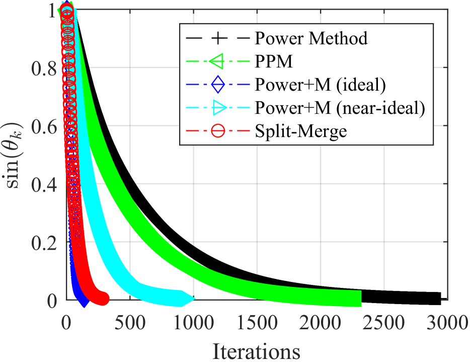
(a) Kuu

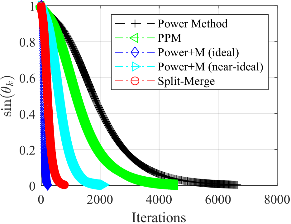
(b) Andrews

(c) thermomech_TC

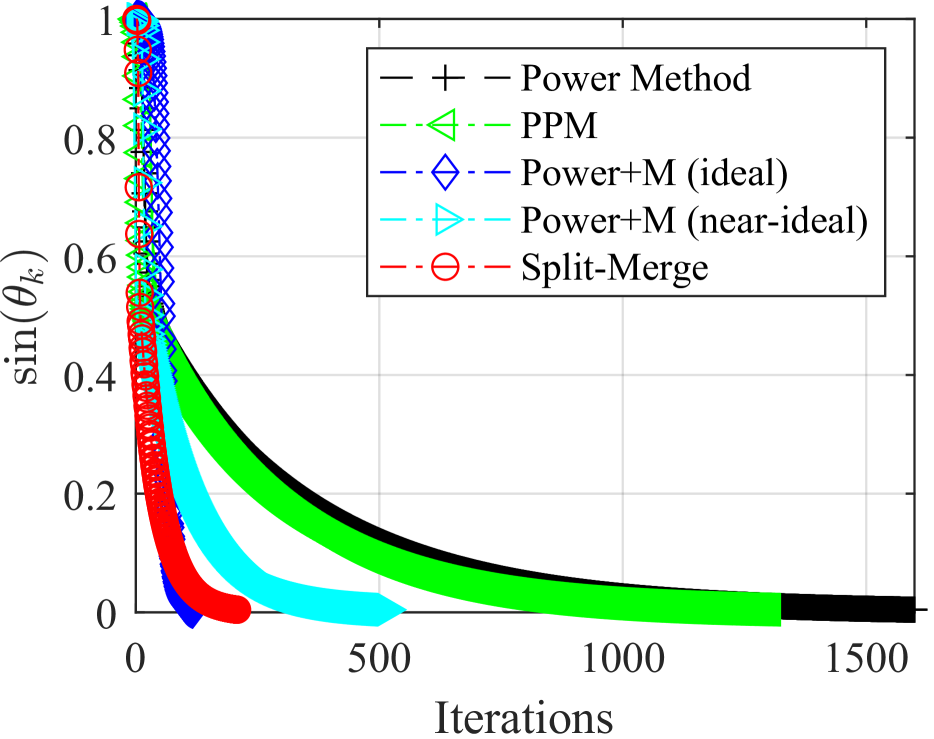
(d) boneS01

Figure 1: Comparison of different methods on four SuiteSparse benchmark matrix datasets. The speed-up achieved by Split-Merge method is highlighted for each dataset: (a) Kuu: 10.78, (b) Andrews: 8.47, (c) thermomech_TC: 8.63, and (d) boneS01: 7.57.

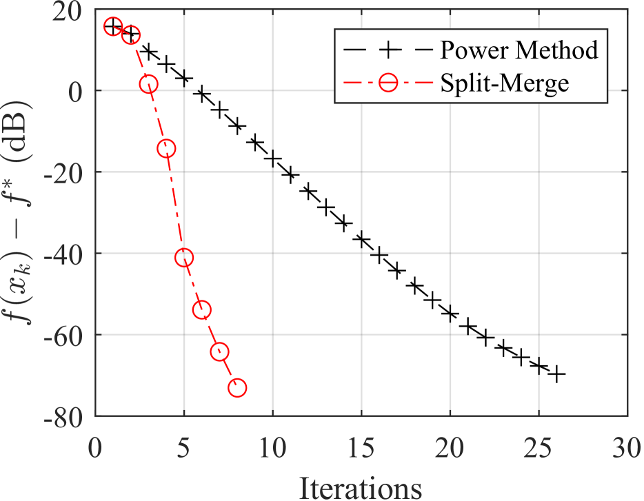
(a) Gisette

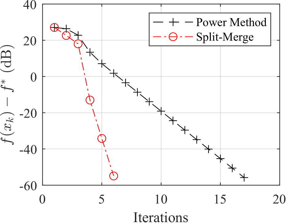
(b) Arcene

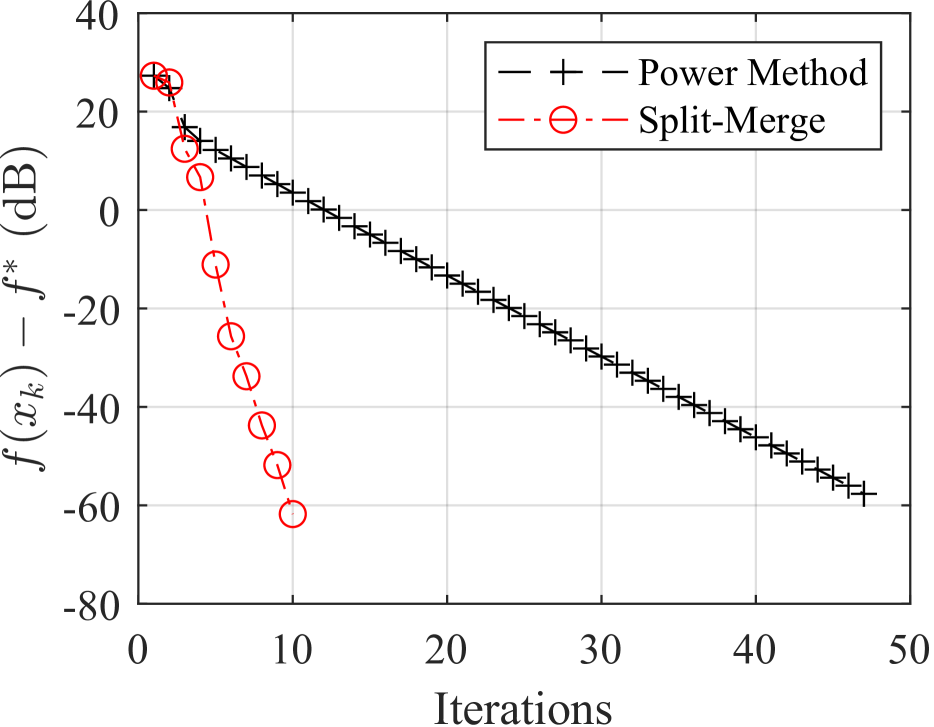
(c) gene expression cancer RNA-Seq

Figure 2: Convergence comparison between the Split-Merge method ($\boldsymbol{v}=\hat{\boldsymbol{v}}$) and the power method ($\boldsymbol{v}=\boldsymbol{0}$) on three UCI Machine Learning datasets. The y-axis shows the difference from the optimal function value $f^{*}=-\frac{\lambda_{1}}{4}$, scaled by $10\log_{10}$ (dB). The speed-up achieved for each dataset is: (a) Gisette: 3.41, (b) Arcene: 2.99, and (c) gene Expression Cancer RNA-Seq: 4.95.

6 Experiments

In this section, we compare the Split-Merge algorithm with the power method Mises & Pollaczek-Geiringer (1929) and its variants: PPM Bai et al. (2021), Power+M Xu et al. (2018), and the Best Ball method Xu et al. (2018), using both synthetic and real-world datasets. Power+M is initialized with the optimal momentum parameter $\beta^{*}={\lambda_{2}^{2}}/{4}$ (denoted as Power+M (ideal)), serving as an ideal baseline among moment-based methods for experimental comparison. However, this optimal spectral knowledge is impractical in real-world applications, making the ideal baseline unattainable in practice. Additionally, we evaluate the performance of our proposed algorithm against Power+M with a perturbed parameter $\beta=0.9\beta^{*}$ (denoted as Power+M (near-ideal)). These comparisons demonstrate the superior efficiency of our algorithm in addressing the eigenvalue problem.

For all algorithm, the initial vector $\boldsymbol{x}_{0}$ is the same, generated using MATLAB’s randn function. All results are averaged over 100 random runs. The stopping criterion is defined as $\sin(\theta_{k})\leq\epsilon$, where $\epsilon=10^{-8}$ and $\theta_{k}$ is the angle between the current iterate $\boldsymbol{x}_{k}$ and the dominant eigenvector $\boldsymbol{u}_{1}$. Alternatively, the algorithm terminates if the number of iterations exceeds 20,000.

The algorithms are evaluated based on two metrics: the number of iterations (denoted as Iter) and computational time (denoted as Time). We also present the speed-up of the Split-Merge algorithm relative to the power method, which is defined as

$$\text{speed-up}=\frac{\text{Time of power method}}{\text{Time of Split-Merge}}.$$

6.1 Synthetic Dataset

We begin with synthetic experiments (details provided in Appendix K) to compare the performance of these methods across different configurations, including variations in matrix dimensions $n$ and eigen-gap values $\Delta$.

Table 1 summarizes the average Iter and Time for various algorithms. As shown, the Split-Merge method or the Power+M (ideal) consistently achieves the best performance across all cases. In practice, however, the optimal parameter $\beta^{*}$ is typically unknown. Additionally, the Power+M method is highly sensitive to the choice of $\beta$: even slight perturbations can significantly degrade its computational efficiency. For instance, when $\Delta=10^{-3}$, the Time of Power+M (near-ideal) is three times that of the Split-Merge method.

The heuristic Best Ball method performs fewer iterations than Power+M (near-ideal) when $\Delta$ is small, but its requirement for multiple matrix-vector products per iteration to estimate the parameter $\beta^{*}$ results in higher overall computational costs. In comparison, the Split-Merge method achieves over a $34\times$ speed-up in runtime compared to the Best Ball method (e.g., $n=4096$, $\Delta=10^{-2}$).

The PPM method fails to converge in certain random runs when $\Delta$ is small, as it relies on local convergence guarantees. These guarantees break down when the spectral prior is inaccurately estimated, leading to reconstruction failures. In contrast, the Split-Merge method does not depend on spectral priors and consistently converges across all experimental cases. It outperforms other baselines in both Iter and Time, achieving over a $9\times$ speed-up compared to the basic Power Method (e.g., $n=2048$, $\Delta=10^{-3}$).

6.2 SuiteSparse Matrix Dataset

We assess the performance of our algorithm using four PSD benchmark problems from the SuiteSparse Matrix Collection Davis & Hu (2011). These matrices vary in size: Kuu ($n=7,102$), Andrews ($n=60,000$), thermomech_TC ($n=102,158$), and boneS01 ($n=127,224$). MATLAB’s eigs function is used to compute the dominant eigenvector of these matrices as the ground truth.

Figure 1 illustrates the convergence behavior of $\sin(\boldsymbol{x}_{k})$ against the number of iterations for different methods. As shown, the Split-Merge method consistently accelerates convergence across all matrix sizes compared to existing methods. Notably, it achieves over a $\boldsymbol{10\times}$ speed-up on the Kuu matrix relative to the power method. For larger matrices, such as Andrews and thermomech_TC, it still delivers significant improvements, with a speed-up exceeding $8\times$.

6.3 Real-World Dataset

To evaluate the performance of the Split-Merge algorithm in the real-world PCA tasks, we apply it to three UCI Machine Learning Repository datasets: Gisette Guyon & Dror (2004b), Arcene Guyon & Dror (2004a), and gene expression cancer RNA-Seq Fiorini (2016). For each dataset, we first normalize the features to have zero mean and unit variance before performing PCA.

Datasets

• Gisette Guyon & Dror (2004b): Consists of 13,500 samples with 5,000 features, designed for handwritten digit recognition tasks.

• Arcene Guyon & Dror (2004a): Comprising 900 samples with 10,000 features, this dataset aims to classify cancerous versus normal patterns in mass-spectrometric data.

• gene expression cancer RNA-Seq Fiorini (2016): Includes 801 samples with 20,531 gene expression features, focusing on cancer classification through gene expression analysis.

Figure 2 depicts the convergence behavior of the objective function $f(\boldsymbol{x}_{k})$ with respect to the number of iterations for the Split-Merge method and the power method. As discussed earlier, from the perspective of the Difference formulation, both the Split-Merge method and the power method can be viewed as special cases within the same algorithmic family, differing only in the selection of $\boldsymbol{v}$. The results in the figure demonstrate that, by optimally choosing $\hat{\boldsymbol{v}}$, the Split-Merge method achieves a speed-up of up to nearly $5\times$ compared to the power method on real-world machine learning datasets.

7 Conclusion

In this work, we introduced a novel Difference formulation for solving eigenvalue problems, marking the first departure from the traditional Quotient formulation. This perspective reinterprets the classical power method as a DCA using only first-order information. To address the power method’s limitations, we proposed a new family of algorithms by exploiting the splitting property of PSD matrices. This family not only includes the power method as a special case but also opens new avenues for studying eigenvalue problems. Within this family, we developed the Split-Merge algorithm, an optimal approach that dynamically selects vectors $\boldsymbol{u}$ and $\boldsymbol{v}$ to maximize the surrogate function’s reduction at each iteration. Notably, the algorithm achieves maximal acceleration while simultaneously merging the decomposed matrices, rendering it decomposition-free. We also provided rigorous convergence analysis, supported by extensive empirical results showing the Split-Merge algorithm consistently outperforms baseline methods across various datasets.

Future work. Our work opens several promising research directions. First, a deeper theoretical analysis of the proposed Difference formulation from an optimization perspective could yield additional insights. Second, investigating the application of quasi-Newton methods and other local optimization techniques to solve the resulting non-convex problem, along with an analysis of their global convergence properties, represents a critical extension.

Impact Statement

This paper presents work whose goal is to advance the field of Machine Learning. There are many potential societal consequences of our work, none which we feel must be specifically highlighted here.

Appendix A Proof of Lemma 2.2

Proof.

By elementary calculus, the function $f(\boldsymbol{x})$ is non-differentiable if and only if $\boldsymbol{x}^{T}\boldsymbol{A}\boldsymbol{x}=0$. If $\boldsymbol{A}$ is PSD, this is equivalent to $\boldsymbol{A}\boldsymbol{x}=\boldsymbol{0}$.

Any PSD matrix $\boldsymbol{A}$ admits a full-rank decomposition $\boldsymbol{A}=\boldsymbol{F}^{T}\boldsymbol{F}$ (see Lemma 4.1). Thus, $\boldsymbol{x}^{T}\boldsymbol{A}\boldsymbol{x}=0$ implies

$$\boldsymbol{x}^{T}\boldsymbol{F}^{T}\boldsymbol{F}\boldsymbol{x}=\left\|\boldsymbol{F}\boldsymbol{x}\right\|^{2}=0,$$

which leads to $\boldsymbol{F}\boldsymbol{x}=\boldsymbol{0}$, and hence $\boldsymbol{Ax}=\boldsymbol{0}$. The converse is also evidently true.

At any differentiable point $\boldsymbol{x}\in\Theta$, the gradient and Hessian of $f(\boldsymbol{x})$ are given by (3) and (4), respectively. ∎

Appendix B Proof of Lemma 2.3

Proof.

A stationary point $\boldsymbol{x}$ of $f\left(\boldsymbol{x}\right)$ satisfies

$$\nabla f\left(\boldsymbol{x}\right)=\boldsymbol{0}.$$

Substituting the expression for $\nabla f\left(\boldsymbol{x}\right)$ from (3) into this condition, we obtain

$$\boldsymbol{Ax}=2\left(\boldsymbol{x}^{T}\boldsymbol{A}\boldsymbol{x}\right)^{\frac{1}{2}}\boldsymbol{x},$$

which implies that $\boldsymbol{x}$ is an eigenvector of $\boldsymbol{A}$ with the associated eigenvalue given by (5). ∎

Appendix C Proof of Theorem 2.4

Proof.

The function $f\left(\boldsymbol{x}\right)$ is coercive, ensuring the existence of global minima. By Lemma 2.3, it follows that the stationary point $\boldsymbol{x}$ corresponding to the eigenvalue $\lambda$ satisfies

$$\left\|\boldsymbol{x}\right\|=\frac{\sqrt{\lambda}}{2},$$

and

$$f\left(\boldsymbol{x}\right)=-\frac{\lambda}{4}.$$

Therefore, we have

$$f\left(\boldsymbol{x}\right)\geq-\frac{\lambda_{1}}{4},\ \forall\boldsymbol{x}\in\mathbb{R}^{n}.$$

The corresponding global minima are aligned with the dominant eigenvector $\boldsymbol{u}_{1}$. ∎

Appendix D Proof of Theorem 2.5

Proof.

By Lemma 2.3, any second-order stationary point $\boldsymbol{x}$ must be an eigenvector of $\boldsymbol{A}$. We now prove by contradiction that all eigenvectors of $\boldsymbol{A}$, except for the dominant eigenvector, are saddle points.

Assume that a second-order stationary point $\boldsymbol{x}$ is an eigenvector associated with an eigenvalue $\lambda<\lambda_{1}$. Let $\boldsymbol{u}_{1}$ be the dominant eigenvector of $\boldsymbol{A}$, corresponding to $\lambda_{1}$, normalized such that $\left\|\boldsymbol{u}_{1}\right\|=1$. Since $\nabla^{2}f\left(\boldsymbol{x}\right)\succeq 0$, it follows that:

$$\boldsymbol{u}_{1}^{T}\nabla^{2}f\left(\boldsymbol{x}\right)\boldsymbol{u}_{1}\geq 0.$$ (27)

Using the orthogonality of eigenvectors, we have $\boldsymbol{x}^{T}\boldsymbol{u}_{1}=0$. Substituting the expression for $\nabla^{2}f\left(\boldsymbol{x}\right)$ in (4) into (27) yields:

$$0\leq 2\boldsymbol{u}_{1}^{T}\boldsymbol{u}_{1}-\frac{\boldsymbol{u}_{1}^{T}\boldsymbol{A}\boldsymbol{u}_{1}}{\left(\boldsymbol{x}^{T}\boldsymbol{A}\boldsymbol{x}\right)^{\frac{1}{2}}}=\frac{2}{\lambda}(\lambda-\lambda_{1})<0,$$

which leads to a contradiction.

Therefore, no eigenvector associated with $\lambda<\lambda_{1}$ can be a second-order stationary point. Hence, the dominant eigenvector is the only global minimum, and all other eigenvectors are saddle points. ∎

Appendix E Proof of Theorem 4.3

Proof.

Using eigenvalue decomposition, it can be readily shown that for any vectors $\boldsymbol{u},\boldsymbol{v}$ satisfying $\|\boldsymbol{u}\|\leq 1$, $\|\boldsymbol{v}\|\leq 1$, and $\boldsymbol{u}^{T}\boldsymbol{v}=0$, the following condition holds:

$$\boldsymbol{I}\succeq\boldsymbol{u}\boldsymbol{u}^{T}+\boldsymbol{v}\boldsymbol{v}^{T}.$$

Applying Lemma 4.1, for any PSD matrix $\boldsymbol{A}$ with a full-rank decomposition $\boldsymbol{A}=\boldsymbol{F}^{T}\boldsymbol{F}$, we have:

$$\boldsymbol{A}=\boldsymbol{F}^{T}\boldsymbol{F}\succeq\boldsymbol{F}^{T}\left(\boldsymbol{u}\boldsymbol{u}^{T}+\boldsymbol{v}\boldsymbol{v}^{T}\right)\boldsymbol{F}.$$

Thus, it follows that:

$$\nabla^{2}f\left(\boldsymbol{x}\right)=2\boldsymbol{I}-\frac{\boldsymbol{F}^{T}\boldsymbol{F}}{\left(\boldsymbol{x}^{T}\boldsymbol{A}\boldsymbol{x}\right)^{\frac{1}{2}}}+\frac{\left(\boldsymbol{Ax}\right)\left(\boldsymbol{Ax}\right)^{T}}{\left(\boldsymbol{x}^{T}\boldsymbol{A}\boldsymbol{x}\right)^{\frac{3}{2}}}\preceq\boldsymbol{H}_{\boldsymbol{x}}(\boldsymbol{u},\boldsymbol{v}).$$

∎

Appendix F Proof of Proposition 4.5

Proof.

Let $\boldsymbol{u}\equiv\frac{\boldsymbol{F}\boldsymbol{x}_{k}}{\|\boldsymbol{F}\boldsymbol{x}_{k}\|}$. For any choice of $\boldsymbol{v}$, we have

$$\boldsymbol{H}_{\boldsymbol{x}_{k}}(\boldsymbol{u},\boldsymbol{v})=2\boldsymbol{I}-\frac{1}{\left(\boldsymbol{x}_{k}^{T}\boldsymbol{A}\boldsymbol{x}_{k}\right)^{\frac{1}{2}}}\boldsymbol{F}^{T}\boldsymbol{v}\left(\boldsymbol{F}^{T}\boldsymbol{v}\right)^{T}\preceq 2\boldsymbol{I}=\nabla^{2}f_{k}(\boldsymbol{x}_{k}).$$

Using the result from Theorem 4.3, it follows that

$$\nabla^{2}f_{k}(\boldsymbol{x}_{k})=2\boldsymbol{I}\succeq\boldsymbol{H}_{\boldsymbol{x}_{k}}(\boldsymbol{u},\boldsymbol{v})\succeq\nabla^{2}f(\boldsymbol{x}_{k}).$$

∎

Appendix G Proof of Theorem 4.6

Proof.

Under the positive definiteness assumption of the matrix $\boldsymbol{H}_{\boldsymbol{x}_{k}}(\boldsymbol{u},\boldsymbol{v})$, for a fixed $\boldsymbol{v}$, we have

$$\hat{\boldsymbol{d}} =\arg\min_{\boldsymbol{d}}\phi_{k}(\boldsymbol{x}_{k}+\boldsymbol{d})$$

$$=\arg\min_{\boldsymbol{d}}\nabla f(\boldsymbol{x}_{k})^{T}\boldsymbol{d}+\frac{1}{2}\boldsymbol{d}^{T}\boldsymbol{H}_{\boldsymbol{x}_{k}}(\boldsymbol{u},\boldsymbol{v})\boldsymbol{d}$$

$$=-\left(\boldsymbol{H}_{\boldsymbol{x}_{k}}(\boldsymbol{u},\boldsymbol{v})\right)^{-1}\nabla f(\boldsymbol{x}_{k}).$$

Substituting into (14), we derive

$$\hat{\boldsymbol{v}}=\arg\max_{\boldsymbol{v}}\frac{1}{2}\nabla f(\boldsymbol{x}_{k})^{T}\left(\boldsymbol{H}_{\boldsymbol{x}_{k}}(\boldsymbol{u},\boldsymbol{v})\right)^{-1}\nabla f(\boldsymbol{x}_{k}),\ \text{s.t.}\ \boldsymbol{v}\in\Omega.$$

By incorporating $\nabla f(\boldsymbol{x})$ from (3) and $\boldsymbol{H}_{\boldsymbol{x}_{k}}(\boldsymbol{u},\boldsymbol{v})^{-1}$ from (12), and applying the condition $\boldsymbol{v}^{T}\boldsymbol{Fx}_{k}=0$, we obtain

$$\hat{\boldsymbol{v}} =\arg\max_{\boldsymbol{v}}\left(2\boldsymbol{x}_{k}-\frac{\boldsymbol{Ax}_{k}}{\left(\boldsymbol{x}_{k}^{T}\boldsymbol{A}\boldsymbol{x}_{k}\right)^{\frac{1}{2}}}\right)^{T}\left(\boldsymbol{I}+\frac{1}{2\sigma(\boldsymbol{x}_{k}^{T}\boldsymbol{A}\boldsymbol{x}_{k})^{\frac{1}{2}}}\boldsymbol{F}^{T}\boldsymbol{v}(\boldsymbol{F}^{T}\boldsymbol{v})^{T}\right)\left(2\boldsymbol{x}_{k}-\frac{\boldsymbol{Ax}_{k}}{\left(\boldsymbol{x}_{k}^{T}\boldsymbol{A}\boldsymbol{x}_{k}\right)^{\frac{1}{2}}}\right),\ \text{s.t.}\ \boldsymbol{v}\in\Omega$$

$$=\arg\max_{\boldsymbol{v}}\frac{\left(\boldsymbol{v}^{T}\boldsymbol{FF}^{T}\boldsymbol{F}\boldsymbol{x}_{k}\right)^{2}}{1-\frac{\boldsymbol{v}^{T}\boldsymbol{FF}^{T}\boldsymbol{v}}{2(\boldsymbol{x}_{k}^{T}\boldsymbol{A}\boldsymbol{x}_{k})^{\frac{1}{2}}}},\ \text{s.t.}\ \boldsymbol{v}\in\Omega.$$

Using the regularization constraint $\boldsymbol{v}^{T}\boldsymbol{v}=\frac{1}{\rho}$, we further simplify to

$$\hat{\boldsymbol{v}} =\arg\max_{\boldsymbol{v}}\frac{\left(\boldsymbol{v}^{T}\boldsymbol{FF}^{T}\boldsymbol{F}\boldsymbol{x}_{k}\right)^{2}}{\rho\boldsymbol{v}^{T}\boldsymbol{v}-\frac{\boldsymbol{v}^{T}\boldsymbol{FF}^{T}\boldsymbol{v}}{2(\boldsymbol{x}_{k}^{T}\boldsymbol{A}\boldsymbol{x}_{k})^{\frac{1}{2}}}},\ \text{s.t.}\ \boldsymbol{v}\in\Omega$$

$$=\arg\max_{\boldsymbol{v}}\frac{\boldsymbol{v}^{T}\boldsymbol{B}\boldsymbol{v}}{\boldsymbol{v}^{T}\boldsymbol{C}\boldsymbol{v}},\ \text{s.t.}\ \boldsymbol{v}\in\Omega.$$

∎

Appendix H Proof of Theorem 5.1

Proof.

The iteration sequence $\{\boldsymbol{x}_{k}\}_{k=0}^{\infty}$ is defined as

$$\boldsymbol{x}_{k}=\boldsymbol{A}^{k}\prod_{m=0}^{k-1}(\zeta_{m}\boldsymbol{I}+\omega_{m}\boldsymbol{A})\boldsymbol{x}_{0}.$$ (28)

Let $\boldsymbol{x}_{0}=\sum_{i=1}^{n}a_{i}\boldsymbol{u}_{i}$, with $\|\boldsymbol{x}_{0}\|=1$. Thus, we have

$$\left|a_{1}\right|=\cos(\theta_{0})\neq 0.$$

Next, by substituting the iterates of $\boldsymbol{x}_{k}$ in (28), we obtain

$$\left|\sin(\theta_{k})\right|^{2} =1-\frac{(\boldsymbol{u}_{1}^{T}\boldsymbol{x}_{k})^{2}}{\left\|\boldsymbol{x}_{k}\right\|^{2}}$$

$$=1-\frac{({\lambda_{1}}^{k}\prod_{m=0}^{k-1}(\zeta_{m}+\omega_{m}\lambda_{1})a_{1})^{2}}{\sum_{i=1}^{n}({\lambda_{i}}^{k}\prod_{m=0}^{k-1}(\zeta_{m}+\omega_{m}\lambda_{i})a_{i})^{2}}$$

$$=\frac{\sum_{i=2}^{n}({\lambda_{i}}^{k}\prod_{m=0}^{k-1}(\zeta_{m}+\omega_{m}\lambda_{i})a_{i})^{2}}{\sum_{i=1}^{n}({\lambda_{i}}^{k}\prod_{m=0}^{k-1}(\zeta_{m}+\omega_{m}\lambda_{i})a_{i})^{2}}$$

$$\leq\frac{\sum_{i=2}^{n}({\lambda_{i}}^{k}\prod_{m=0}^{k-1}(\zeta_{m}+\omega_{m}\lambda_{i})a_{i})^{2}}{({\lambda_{1}}^{k}\prod_{m=0}^{k-1}(\zeta_{m}+\omega_{m}\lambda_{1})a_{1})^{2}}$$

$$=\frac{1}{a_{1}^{2}}\sum_{i=2}^{n}(\frac{\lambda_{i}}{\lambda_{1}})^{2k}\prod_{m=0}^{k-1}\left|\frac{\zeta_{m}+\omega_{m}\lambda_{i}}{\zeta_{m}+\omega_{m}\lambda_{1}}\right|^{2}a_{i}^{2}$$

$$\leq\frac{1}{a_{1}^{2}}(\frac{\lambda_{2}}{\lambda_{1}})^{2k}\sum_{i=2}^{n}\prod_{m=0}^{k-1}\left|\frac{\zeta_{m}+\omega_{m}\lambda_{i}}{\zeta_{m}+\omega_{m}\lambda_{1}}\right|^{2}a_{i}^{2}.$$

If we have

$$\left|\frac{\zeta_{k}+\omega_{k}\lambda_{j}}{\zeta_{k}+\omega_{k}\lambda_{1}}\right|\leq\delta\leq 1,\quad j=2,3,\cdots,n,\quad k=0,1,\cdots,$$

we obtain

$$\left|\sin(\theta_{k})\right|^{2} \leq\frac{\sum_{i=2}^{n}a_{i}^{2}}{a_{1}^{2}}(\frac{\lambda_{2}}{\lambda_{1}})^{2k}\delta^{2k}$$ (29)

$$=\frac{1-a_{1}^{2}}{a_{1}^{2}}(\frac{\lambda_{2}}{\lambda_{1}})^{2k}\delta^{2k}$$

$$=\tan(\theta_{0})^{2}(\frac{\lambda_{2}}{\lambda_{1}})^{2k}\delta^{2k}.$$

This confirms the validity of (22).

Next, by substituting (28) into the Rayleigh quotient $r(\boldsymbol{x}_{k})$, we obtain:

$$r(\boldsymbol{x}_{k})=\frac{\sum_{i=1}^{n}\lambda_{i}({\lambda_{i}}^{k}\prod_{m=0}^{k-1}(\zeta_{m}+\omega_{m}\lambda_{i})a_{i})^{2}}{\sum_{i=1}^{n}({\lambda_{i}}^{k}\prod_{m=0}^{k-1}(\zeta_{m}+\omega_{m}\lambda_{i})a_{i})^{2}}.$$

Thus, we have the following inequality:

$$\left|r(\boldsymbol{x}_{k})-\lambda_{1}\right| =\left|\frac{\sum_{i=2}^{n}(\lambda_{i}-\lambda_{1})({\lambda_{i}}^{k}\prod_{m=0}^{k-1}(\zeta_{m}+\omega_{m}\lambda_{i})a_{i})^{2}}{\sum_{i=1}^{n}({\lambda_{i}}^{k}\prod_{m=0}^{k-1}(\zeta_{m}+\omega_{m}\lambda_{i})a_{i})^{2}}\right|$$

$$\leq\frac{\sum_{i=2}^{n}\left|\lambda_{i}-\lambda_{1}\right|({\lambda_{i}}^{k}\prod_{m=0}^{k-1}(\zeta_{m}+\omega_{m}\lambda_{i})a_{i})^{2}}{\sum_{i=1}^{n}({\lambda_{i}}^{k}\prod_{m=0}^{k-1}(\zeta_{m}+\omega_{m}\lambda_{i})a_{i})^{2}}$$

$$\leq(\lambda_{1}-\lambda_{n})\frac{\sum_{i=2}^{n}({\lambda_{i}}^{k}\prod_{m=0}^{k-1}(\zeta_{m}+\omega_{m}\lambda_{i})a_{i})^{2}}{\sum_{i=1}^{n}({\lambda_{i}}^{k}\prod_{m=0}^{k-1}(\zeta_{m}+\omega_{m}\lambda_{i})a_{i})^{2}}$$

$$=(\lambda_{1}-\lambda_{n})\left|\sin(\theta_{k})\right|^{2}.$$

Substituting (29) into this expression verifies that (23) holds true. ∎

Appendix I Justification for $\rho_{k}\equiv 1$ and its Convergence Behavior

This section justifies setting $\rho_{k}\equiv 1$ and investigates its effect on the convergence behavior of the Split-Merge algorithm.

We demonstrate that when $\boldsymbol{x}_{k}$ converges to $\boldsymbol{u}_{1}$ and $\mu_{k}$ approaches $\lambda_{1}$, the vector $\boldsymbol{z}_{k}=\boldsymbol{Ax}_{k}-\frac{\boldsymbol{x}_{k}^{T}\boldsymbol{A}^{2}\boldsymbol{x}_{k}}{\boldsymbol{x}_{k}^{T}\boldsymbol{A}\boldsymbol{x}_{k}}\boldsymbol{x}_{k}$ becomes nearly orthogonal to $\boldsymbol{x}_{k}$ (i.e., $\boldsymbol{z}_{k}^{T}\boldsymbol{x}_{k}\approx 0$). This implies that $\boldsymbol{z}_{k}$ lies in the subspace spanned by $\left\{\boldsymbol{u}_{2},\cdots\boldsymbol{u}_{n}\right\}$. Consequently, $\boldsymbol{v}=\boldsymbol{Fz}_{k}$ lies in the subspace spanned by $\left\{\boldsymbol{Fu}_{2},\cdots\boldsymbol{Fu}_{n}\right\}$, leading to

$$\frac{\boldsymbol{v}^{T}\boldsymbol{FF}^{T}\boldsymbol{v}}{\boldsymbol{v}^{T}\boldsymbol{v}}\in\left[\lambda_{n},\lambda_{2}\right].$$

When $\rho_{k}\equiv 1$, the quantity $\sigma_{k}=1-\frac{1}{\mu_{k}}\cdot\frac{\boldsymbol{v}^{T}\boldsymbol{FF}^{T}\boldsymbol{v}}{\boldsymbol{v}^{T}\boldsymbol{v}}$ approximates $1-\frac{1}{\lambda_{1}}\cdot\frac{\boldsymbol{v}^{T}\boldsymbol{FF}^{T}\boldsymbol{v}}{\boldsymbol{v}^{T}\boldsymbol{v}}$, which is strictly positive, thereby satisfying the positive-definiteness condition in (25). Furthermore, the term $-\frac{\zeta_{k}}{\omega_{k}}=\frac{\boldsymbol{x}_{k}^{T}\boldsymbol{A}^{2}\boldsymbol{x}_{k}}{\boldsymbol{x}_{k}^{T}\boldsymbol{A}\boldsymbol{x}_{k}}-\mu_{k}\sigma_{k}$ approximates $\frac{\boldsymbol{v}^{T}\boldsymbol{FF}^{T}\boldsymbol{v}}{\boldsymbol{v}^{T}\boldsymbol{v}}$, which lies within the range $\left[\lambda_{n},\lambda_{2}\right]$. Empirical results indicate that this value tends to cluster around ${(\lambda_{2}+\lambda_{n})}/{2}$, as shown in Figure 3.

To ensure strict convergence, we propose a two-stage approach. In the first stage, $\rho_{k}$ is fixed at $1$ to maximize acceleration. In the second stage, $\rho_{k}$ is adjusted to meet the convergence condition in (26). Notably, in all experimental cases, the algorithm terminates within the first stage, further supporting the validity of these findings.

(a) $\lambda_{1}=0.8$

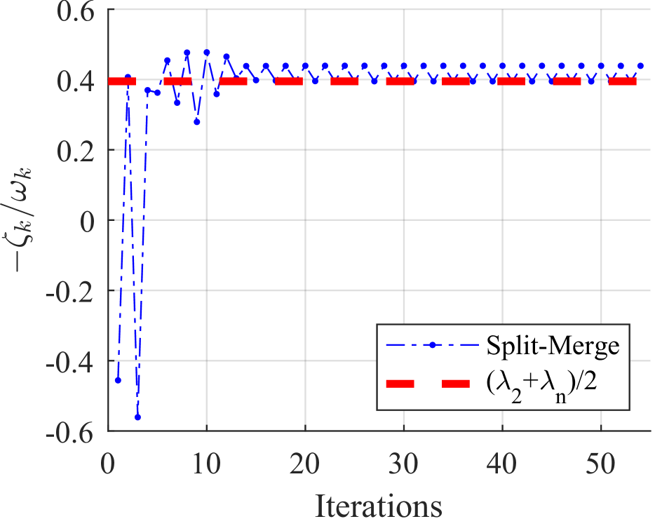
(b) $\lambda_{1}=0.5$

Figure 3: Convergence behavior of the value $-\frac{\zeta_{k}}{\omega_{k}}$ when $\rho_{k}\equiv 1$. Experiments with synthetic PSD matrices ($n=1024$, $\Delta=10^{-2}$) and varying dominant eigenvalues: (a) $\lambda_{1}=0.8$, (b) $\lambda_{1}=0.5$.

Appendix J Detailed Derivation of Some Formulas

J.1 Equivalent Condition for the Positive Definiteness of the Matrix $\boldsymbol{H}_{\boldsymbol{x}_{k}}(\boldsymbol{u},\boldsymbol{v})$

When $\boldsymbol{u}\equiv\frac{\boldsymbol{F}\boldsymbol{x}_{k}}{\|\boldsymbol{F}\boldsymbol{x}_{k}\|}$, the matrix

$$\boldsymbol{H}_{\boldsymbol{x}_{k}}(\boldsymbol{u},\boldsymbol{v})=2\boldsymbol{I}-\frac{1}{\left(\boldsymbol{x}_{k}^{T}\boldsymbol{A}\boldsymbol{x}_{k}\right)^{\frac{1}{2}}}\boldsymbol{F}^{T}\boldsymbol{v}\left(\boldsymbol{F}^{T}\boldsymbol{v}\right)^{T}$$

has eigenvalues that are all equal to 2, except for one given by $2-\frac{\boldsymbol{v}^{T}\boldsymbol{FF}^{T}\boldsymbol{v}}{\left(\boldsymbol{x}_{k}^{T}\boldsymbol{A}\boldsymbol{x}_{k}\right)^{\frac{1}{2}}}$.

Therefore, the matrix $\boldsymbol{H}_{\boldsymbol{x}_{k}}(\boldsymbol{u},\boldsymbol{v})\succ 0$, if and only if

$$2-\frac{\boldsymbol{v}^{T}\boldsymbol{FF}^{T}\boldsymbol{v}}{\left(\boldsymbol{x}_{k}^{T}\boldsymbol{A}\boldsymbol{x}_{k}\right)}>0.$$

In other words, $\sigma>0$.

J.2 Derivation of the Inequality (17)

Noting that the matrices $\boldsymbol{A}=\boldsymbol{F}^{T}\boldsymbol{F}$ and $\boldsymbol{FF}^{T}$ share the same non-zero eigenvalues, we utilize the following inequality:

$$\boldsymbol{v}^{T}\boldsymbol{FF}^{T}\boldsymbol{v}\leq\frac{1}{\rho}\lambda_{1},$$

where $\lambda_{1}$ denotes the dominant eigenvalue of $\boldsymbol{FF}^{T}$. Based on this, we derive the bound:

$$\frac{\boldsymbol{v}^{T}\boldsymbol{B}\boldsymbol{v}}{\boldsymbol{v}^{T}\boldsymbol{C}\boldsymbol{v}}=\frac{\left(\boldsymbol{v}^{T}\boldsymbol{FF}^{T}\boldsymbol{F}\boldsymbol{x}_{k}\right)^{2}}{1-\frac{\boldsymbol{v}^{T}\boldsymbol{FF}^{T}\boldsymbol{v}}{2(\boldsymbol{x}_{k}^{T}\boldsymbol{A}\boldsymbol{x}_{k})^{\frac{1}{2}}}}\leq\frac{\left(\boldsymbol{v}^{T}\boldsymbol{FF}^{T}\boldsymbol{F}\boldsymbol{x}_{k}\right)^{2}}{1-\frac{\lambda_{1}}{2\rho(\boldsymbol{x}_{k}^{T}\boldsymbol{A}\boldsymbol{x}_{k})^{\frac{1}{2}}}}.$$

J.3 Derivation of the Update Formula (19)

Substituting the solution in (18) into the update formula in (13) results in the following expression:

$$\boldsymbol{x}_{k+1} =\frac{1}{2(\boldsymbol{x}_{k}^{T}\boldsymbol{A}\boldsymbol{x}_{k})^{\frac{1}{2}}}\boldsymbol{Ax}_{k}+\frac{1}{4\sigma\rho(\boldsymbol{x}_{k}^{T}\boldsymbol{A}\boldsymbol{x}_{k})}\cdot\frac{\left(\boldsymbol{A}^{2}\boldsymbol{x}_{k}-\frac{\boldsymbol{x}_{k}^{T}\boldsymbol{A}^{2}\boldsymbol{x}_{k}}{\boldsymbol{x}_{k}^{T}\boldsymbol{A}\boldsymbol{x}_{k}}\boldsymbol{Ax}_{k}\right)^{T}\boldsymbol{Ax}_{k}}{\left\|\boldsymbol{FF}^{T}\boldsymbol{F}\boldsymbol{x}_{k}-\frac{\boldsymbol{x}_{k}^{T}\boldsymbol{A}^{2}\boldsymbol{x}_{k}}{\boldsymbol{x}_{k}^{T}\boldsymbol{A}\boldsymbol{x}_{k}}\boldsymbol{Fx}_{k}\right\|^{2}}\cdot\left(\boldsymbol{A}^{2}\boldsymbol{x}_{k}-\frac{\boldsymbol{x}_{k}^{T}\boldsymbol{A}^{2}\boldsymbol{x}_{k}}{\boldsymbol{x}_{k}^{T}\boldsymbol{A}\boldsymbol{x}_{k}}\boldsymbol{Ax}_{k}\right).$$

It is important to note that

$$\left(\boldsymbol{A}^{2}\boldsymbol{x}_{k}-\frac{\boldsymbol{x}_{k}^{T}\boldsymbol{A}^{2}\boldsymbol{x}_{k}}{\boldsymbol{x}_{k}^{T}\boldsymbol{A}\boldsymbol{x}_{k}}\boldsymbol{Ax}_{k}\right)^{T}\boldsymbol{Ax}_{k}=\left\|\boldsymbol{FF}^{T}\boldsymbol{F}\boldsymbol{x}_{k}-\frac{\boldsymbol{x}_{k}^{T}\boldsymbol{A}^{2}\boldsymbol{x}_{k}}{\boldsymbol{x}_{k}^{T}\boldsymbol{A}\boldsymbol{x}_{k}}\boldsymbol{Fx}_{k}\right\|^{2}=\boldsymbol{x}_{k}^{T}\boldsymbol{A}^{3}\boldsymbol{x}_{k}-\frac{\left(\boldsymbol{x}_{k}^{T}\boldsymbol{A}^{2}\boldsymbol{x}_{k}\right)^{2}}{\boldsymbol{x}_{k}^{T}\boldsymbol{A}\boldsymbol{x}_{k}}.$$

Therefore, we derive the update formula in (19).

Appendix K Synthetic Dataset Generation

The synthetic PSD matrix $\boldsymbol{A}\in\mathbb{R}^{n\times n}$, with a randomly generated spectrum (denoted as $\mathtt{spec}$), is constructed as follows:

$$\boldsymbol{A}=\boldsymbol{U}\boldsymbol{D}\boldsymbol{U}^{T},$$

where $\boldsymbol{U}$ is an orthogonal matrix obtained using the MATLAB’s randn and qr functions, and $\boldsymbol{D}=\operatorname{diag}(\mathtt{spec})$ is diagonal matrix with $\mathtt{spec}=(\lambda_{1},\lambda_{2},\cdots,\lambda_{n})$. In this setup, $\lambda_{1}=1$, $\lambda_{2}=\lambda_{1}-\Delta$, and the remaining eigenvalues $\lambda_{3},\ldots,\lambda_{n}$ form a decreasing sequence generated randomly using MATLAB’s rand function.

References

• Austin et al. (2024) Austin, C., Pollock, S., and Zhu, Y. Dynamically accelerating the power iteration with momentum. Numerical Linear Algebra with Applications, 31(6):e2584, 2024.
• Bai et al. (2021) Bai, Z.-Z., Wu, W.-T., and Muratova, G. V. The power method and beyond. Applied Numerical Mathematics, 164:29–42, 2021.
• Boyd & Vandenberghe (2004) Boyd, S. and Vandenberghe, L. Convex optimization. Cambridge University Press, 2004.
• Davis & Hu (2011) Davis, T. A. and Hu, Y. The university of florida sparse matrix collection. ACM Transactions on Mathematical Software (TOMS), 38(1):1–25, 2011.
• Fiorini (2016) Fiorini, S. gene expression cancer RNA-Seq. UCI Machine Learning Repository, 2016. URL https://doi.org/10.24432/C5R88H.
• Golub & Van Loan (2013) Golub, G. H. and Van Loan, C. F. Matrix computations. Johns Hopkins University Press, 2013.
• Greenacre et al. (2022) Greenacre, M., Groenen, P. J., Hastie, T., d’Enza, A. I., Markos, A., and Tuzhilina, E. Principal component analysis. Nature Reviews Methods Primers, 2(1):100, 2022.
• Guyon & Dror (2004a) Guyon, Isabelle, G. S. B.-H. A. and Dror, G. Arcene. UCI Machine Learning Repository, 2004a. URL https://doi.org/10.24432/C58P55.
• Guyon & Dror (2004b) Guyon, Isabelle, G. S. B.-H. A. and Dror, G. Gisette. UCI Machine Learning Repository, 2004b. URL https://doi.org/10.24432/C5HP5B.
• Horn & Johnson (2012) Horn, R. A. and Johnson, C. R. Matrix analysis. Cambridge University Press, 2012.
• Knyazev (2001) Knyazev, A. V. Toward the optimal preconditioned eigensolver: Locally optimal block preconditioned conjugate gradient method. SIAM Journal on Scientific Computing, 23(2):517–541, 2001.
• Kuczyński & Woźniakowski (1992) Kuczyński, J. and Woźniakowski, H. Estimating the largest eigenvalue by the power and Lanczos algorithms with a random start. SIAM Journal on Matrix Analysis and Applications, 13(4):1094–1122, 1992.
• Le Thi & Pham Dinh (2018) Le Thi, H. A. and Pham Dinh, T. DC programming and DCA: thirty years of developments. Mathematical Programming, 169(1):5–68, 2018.
• Lee et al. (2013) Lee, J., Kim, S., Lebanon, G., and Singer, Y. Local low-rank matrix approximation. In Dasgupta, S. and McAllester, D. (eds.), Proceedings of the 30th International Conference on Machine Learning (ICML 2013), pp.  82–90, Atlanta, Georgia, USA, 2013. PMLR.
• Lin & Cohen (2010) Lin, F. and Cohen, W. W. Power iteration clustering. In Fürnkranz, J. and Joachims, T. (eds.), Proceedings of the 27th International Conference on Machine Learning (ICML 2010), pp. 655–662, Haifa, Israel, 2010. Omnipress.
• Mises & Pollaczek-Geiringer (1929) Mises, R. and Pollaczek-Geiringer, H. Praktische verfahren der gleichungsauflösung. ZAMM-Journal of Applied Mathematics and Mechanics/Zeitschrift für Angewandte Mathematik und Mechanik, 9(1):58–77, 1929.
• Moler & Stewart (1973) Moler, C. B. and Stewart, G. W. An algorithm for generalized matrix eigenvalue problems. SIAM Journal on Numerical Analysis, 10(2):241–256, 1973.
• Ostrowski (1958) Ostrowski, A. M. On the convergence of the Rayleigh quotient iteration for the computation of the characteristic roots and vectors. I. Archive for Rational Mechanics and Analysis, 1(1):233–241, 1958.
• Page et al. (1999) Page, L., Brin, S., Motwani, R., and Winograd, T. The pagerank citation ranking: Bringing order to the web. Technical report, Stanford InfoLab, 1999.
• Parikh et al. (2014) Parikh, N., Boyd, S., et al. Proximal algorithms. Foundations and trends® in Optimization, 1(3):127–239, 2014.
• Parlett (1998) Parlett, B. N. The symmetric eigenvalue problem. SIAM, Philadelphia, PA, 1998.
• Polyak (1964) Polyak, B. T. Some methods of speeding up the convergence of iteration methods. Ussr Computational Mathematics and Mathematical Physics, 4(5):1–17, 1964.
• Rabbani et al. (2022) Rabbani, T., Jain, A., Rajkumar, A., and Huang, F. Practical and fast momentum-based power methods. In Bruna, J., Hesthaven, J., and Zdeborova, L. (eds.), Proceedings of the 2nd Mathematical and Scientific Machine Learning Conference (MSML 2022), pp.  721–756. PMLR, 2022.
• Rayleigh (1896) Rayleigh, J. W. S. B. The theory of sound, volume 2. Macmillan, 1896.
• Sherman & Morrison (1950) Sherman, J. and Morrison, W. J. Adjustment of an inverse matrix corresponding to a change in one element of a given matrix. The Annals of Mathematical Statistics, 21(1):124–127, 1950.
• Sun et al. (2016) Sun, Y., Babu, P., and Palomar, D. P. Majorization-minimization algorithms in signal processing, communications, and machine learning. IEEE Transactions on Signal Processing, 65(3):794–816, 2016.
• Tao et al. (1986) Tao, P. D. et al. Algorithms for solving a class of nonconvex optimization problems. Methods of subgradients. In North-Holland Mathematics Studies, volume 129, pp. 249–271. Elsevier, 1986.
• Xu et al. (2018) Xu, P., He, B., De Sa, C., Mitliagkas, I., and Re, C. Accelerated stochastic power iteration. In Storkey, A. and Perez-Cruz, F. (eds.), Proceedings of the 21st International Conference on Artificial Intelligence and Statistics (AISTATS 2018), pp.  58–67. PMLR, 2018.