MAP-based Problem-Agnostic diffusion model for Inverse Problems

Abstract

Diffusion models have indeed shown great promise in solving inverse problems in image processing. In this paper, we propose a novel, problem-agnostic diffusion model called the maximum a posteriori (MAP)-based guided term estimation method for inverse problems. We divide the conditional score function into two terms according to Bayes’ rule: the unconditional score function and the guided term. We design the MAP-based guided term estimation method, while the unconditional score function is approximated by an existing score network. To estimate the guided term, we base on the assumption that the space of clean natural images is inherently smooth, and introduce a MAP estimate of the $t$-th latent variable. We then substitute this estimation into the expression of the inverse problem and obtain the approximation of the guided term. We evaluate our method extensively on super-resolution, inpainting, and denoising tasks, and demonstrate comparable performance to DDRM, DMPS, DPS and $\Pi$GDM.

[label1]organization=Library, Shandong University, addressline=No. 180 West Culture Road, city=Weihai, postcode=264209, state=Shandong, country=China [label2]organization=School of Mathematics and Statistics & Hubei Key Laboratory of Engineering Modeling and Scientific Computing & Institute of Interdisciplinary Research for Mathematics and Applied Science, Huazhong University of Science and Technology, addressline=No. 1037 Luoyu road, city=Wuhan, postcode=430074, state=Hubei, country=China [label3]organization=Dapartment of Basic Sciences, Dalian University of Science and Technology, addressline=No. 999-26 Harbor Road, city=Dalian, postcode=116052, state=Liaoning, country=China

[label4]organization=School of Computer Science and Technology, Harbin Institute of Technology, addressline=No. 2 West Culture Road, city=Weihai, postcode=264209, state=Shandong, country=China [label5]organization=School of Artificial Intelligence, Dalian University of Technology, addressline=No. 2 Lingong Road, city=Dalian, postcode=116081, state=Liaoning, country=China

1 Introduction

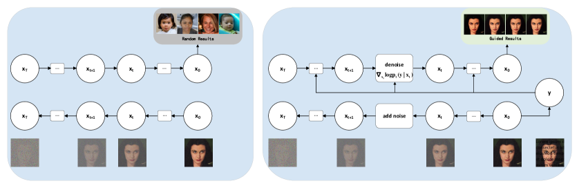
Figure 1: Illustrations of the classical diffusion model (Left) and our proposed method for a specific inverse problem (Right).

Diffusion models have demonstrated their power as both generative models and unsupervised inverse problem solvers, as evidenced by recent research [1, 2, 3, 4]. Owing to their capacity to effectively model complex data distributions and their ability to be trained without relying on specific problem formulations, these models hold great promise and versatility for future research and practical applications across a wide range of domains. Compared to Generative Adversarial Networks (GANs), another popular class of generative models, diffusion models are less prone to mode-collapse and training instabilities. Additionally, diffusion models are more interpretable and provide a natural trade-off between sample quality and diversity.

The diffusion model comprises two diffusion processes. The first is the forward diffusion, also known as the noising process, which drives any data distribution to a tractable distribution by adding noise to the data. The second is the backward diffusion, also known as the denoising process, which sequentially removes noise from noisy data to generate realistic samples. For completeness, we illustrate the procedure in the left subfigure of Figure 1.

The core of diffusion models is the score function, which represents the gradient of the log-density of the data distribution. When solving inverse problems, a conditional score function $\nabla_{\mathbf{x}}\log p(\mathbf{x}|y)$ is applied, where $y$ is the given input and $\mathbf{x}$ is the desired recovery.

There are two main approaches to solving inverse problems using diffusion models. The first is to train a problem-specific, conditional diffusion model for a particular inverse problem. The second approach uses a pre-trained, problem-agnostic diffusion model and combines it with the measurement process via Bayes’ rule. After accessing measurement observations $y$, we can recover $\mathbf{x}$ by either performing maximum a posteriori estimation or posterior sampling over the posterior distribution $p(\mathbf{x}|y)$ via Bayes’ rule. This plug-and-play technique allows the diffusion model to be applied to a wide range of inverse problems without the need for problem-specific training.

There are some existing works based on the problem-agnostic diffusion models, including Denoising Diffusion Restoration Models [5], Diffusion Posterior Sampling [6], Pseudoinverse-Guided Diffusion Models [7], Diffusion Model Based Posterior Sampling [8] and others. Unfortunately, there are some assumptions on distribution. We defer the detailed comparisons to Section 2. In this work, we focus on the second approach and present a novel maximum a posteriori (MAP)-based guided term estimation method for inverse problems. We base on the assumption that the space of clean natural images is inherently smooth, and introduce a MAP estimate of the $t$-th latent variable. We then substitute this estimation into the expression of the inverse problem and obtain the approximation of the guided term.

Our key contributions are as follows:

We introduce a novel MAP-based guided term estimation method for inverse problems. To the best of our knowledge, we are the first to incorporate the prior distribution of natural images into a diffusion model.

Our proposed method is a novel, problem-agnostic diffusion model. We represent the conditional score function as the unconditional score function and the guided term. We design the MAP-based guided term estimation method, while the unconditional score function is approximated by an existing score network.

We extensively evaluate our method on several inverse problems, including super-resolution, inpainting, and denoising. The results demonstrate that our approach achieves comparable performance compared to state-of-the-art approaches.

2 Related Works

Diffusion models [9, 10, 2] have indeed shown great promise in solving inverse problems in image processing [11, 12, 13, 14, 15], where the goal is to recover the original high-quality image from observed, often degraded or incomplete, measurement data [16, 17, 18, 11].

Prior probability models are a fundamental component of many image processing problems. Kadkhodaie and Simoncelli [11] developed a stochastic coarse-to-fine gradient ascent procedure for drawing high-probability samples from the implicit prior to address linear inverse problems. On the other hand, Jalal et al. [12] trained a generative prior on brain scans from the fastMRI dataset and showed that posterior sampling via Langevin dynamics achieved high-quality reconstructions.

Choi et al. [1] proposed the Iterative Latent Variable Refinement (ILVR) method to guide the generative process in DDPM [10] to generate high-quality images based on a given reference image. Unfortunately, this iterative process can accumulate errors, causing the solution path to deviate from the original manifold. To overcome this issue, Chung et al. [4] proposed the MCG method, which introduced additional correction terms inspired by manifold constraints. The objective was to ensure that the iterative process remains closer to the original manifold.

Kawar et al. [5] introduced the DDRM method, which utilized DDPM to address linear inverse problems through matrix singular value decomposition. However, the performance was not satisfactory when the amount of measurement data was insufficient. To overcome this shortcoming, Meng and Kabashima proposed the DMPS method [8] based on the assumption $p(\mathbf{x}_{0}|\mathbf{x}_{t})\propto p(\mathbf{x}_{t}|\mathbf{x}_{0})$, which measured diffusion model guidance based on reconstruction guidance.

Chung et al. developed the DPS method [6] by assuming $\nabla^{2}_{\mathbf{x}_{0}}\log p(\mathbf{x}_{0}),\ \nabla^{2}_{\mathbf{x}_{t}}\log p(\mathbf{x}_{t})\simeq 0$, which effectively handled general noisy nonlinear inverse problems by incorporating the Laplace operator. Song et al. introduced the $\Pi$GDM method [7] based on the assumption $p_{t}(\mathbf{x}_{0}|\mathbf{x}_{t})$ almost a normal distribution, which employed pseudo-inverse guidance by reversing the measurement model to enhance the approximation of guidance.

The paper named MPGD [15] was grounded in the linear subspace manifold hypothesis. It proposed that $p(\mathbf{x}_{t})$ was probabilistically concentrated on a $(d-1)$-dimensional manifold. Building on this proposition, the authors introduced an optimization problem involving tangent spaces and established the relationship between $\mathbf{x}_{t-1}$ and $\mathbf{x}_{0},\mathbf{x}_{t}$.

Besides the methods documented above, natural image priors have been employed for image restoration tasks [19, 20, 21]. Arjomand et al. presented a method [19] based on an image prior that is directly based on an estimate of the natural image probability distribution. Inspired by the work of Arjomand et al. [19], we attempt to perform the diffusion posterior sampling process by incorporating the smooth prior.

3 Proposed Approach

Suppose we have measurements $y\in R^{m}$ of some image $\mathbf{x_{0}}\in R^{n}$, the linear inverse problem can be expressed as follows:

$$y=H\mathbf{x_{0}}+z,$$ (3.1)

where $H\in R^{m\times n}$ is the known measurement matrix, and $z\sim\mathcal{N}(0,\sigma_{y}^{2}I)$ is a Gaussian noise with mean 0 and standard deviation $\sigma_{y}$. We aim to solve the inverse problem and recover $\mathbf{x_{0}}\in R^{n}$ from the measurements $y$.

For the above inverse problem, we focus on the diffusion model and use the problem-specific score $\nabla_{\mathbf{x}}\log p(\mathbf{x}|y)$ instead. One method is to train the problem-specific score associated with diffusion model by paired sample $(\mathbf{x},y)$. The other one is to divide the problem-specific score into two terms. Specifically, we have $p(\mathbf{x}|y)\propto p(\mathbf{x})\cdot p(y|\mathbf{x})$ by Bayes’ rule. Therefore, the posterior score distribution $\nabla_{\mathbf{x}}\log p(\mathbf{x}|y)$ can be decomposed into two terms:

$$\nabla_{\mathbf{x}}\log p(\mathbf{x}|y)=\nabla_{\mathbf{x}}\log p(\mathbf{x})+\nabla_{\mathbf{x}}\log p(y|\mathbf{x}).$$ (3.2)

The first term can be approximated by the existing score network $\mathbf{S}_{\theta}(\mathbf{x},t)$. Consequently, the primary task of estimating the problem-specific score is now focused on computing the second term, which is referred to as the guided term.

In the subsequent subsections, we first provide an overview of the score-based methods, which is then followed by our proposed approach for estimating the MAP-based guided term.

3.1 Overview of Score-based Models

In [2], the forward SDE process of diffusion model can be formalized as the Itô stochastic differential equation

$$d\mathbf{x}_{t}=f(\mathbf{x}_{t},t)dt+g(\mathbf{x}_{t},t)d\omega_{t},$$

where $\omega_{t}$ is the standard Wiener process. When $f(\mathbf{x}_{t},t)=-\frac{1}{2}\beta_{t}\mathbf{x}_{t}$ and $g(\mathbf{x}_{t},t)=\sqrt{\beta_{t}}$, it corresponds to the Variance-Preserving Model (VP-SDE), where $\beta_{t}$ is a non-negative continuous function about $t$. Let $p_{0}(\mathbf{x}_{0})$ be the data distribution and $p_{t}(\mathbf{x}_{t})$ be the distribution obtained by adding Gaussian noise to $p_{0}(\mathbf{x}_{0})$ with $p(\mathbf{x}_{t},t|\mathbf{x}_{0},0)=\mathcal{N}(\mathbf{x}_{t}|\sqrt{1-\zeta_{t}}\mathbf{x}_{0},\zeta_{t}I)$, where $\zeta_{t}=1-e^{-\int^{t}_{0}\beta_{t}dt}$.

In diffusion-based generative models, one estimates the score function $\nabla_{\mathbf{x}_{t}}\log p(\mathbf{x}_{t},t)$ by a neural network $\mathbf{S}_{\theta}(\mathbf{x}_{t},t)$. We have the following representation

$$\frac{-\mathbf{S}_{\theta}(\mathbf{x}_{t},t)}{\sqrt{\zeta_{t}}}\overset{model}{\approx}\nabla_{\mathbf{x}_{t}}\log p(\mathbf{x}_{t},t)\underset{t\neq 0}{\overset{almost\ equal}{\approx}}\nabla_{\mathbf{x}_{t}}\log p(\mathbf{x}_{t},t|\mathbf{x}_{0},0)=-\frac{\mathbf{x}_{t}-\sqrt{1-\zeta_{t}}\mathbf{x}_{0}}{\zeta_{t}},$$

where the almost equal equality is from [22]. As score-based generative models, the score function of diffusion models is approximated with a neural network $\mathbf{S}_{\theta}(\mathbf{x}_{t},t)$, trained with the denoising score matching objective [23]. Once the score is available, solutions can be obtained by solving the SDE or ODE. Throughout of the paper, we use the Variance-Preserving SDE [2], which is equivalent to Denoising Diffusion Probabilistic Models (DDPM) [10].

3.2 MAP-based Guided Term Estimation

In the diffusion model, we need to estimate the problem-specific score function $\nabla_{\mathbf{x}_{t}}\log p(\mathbf{x}_{t}|y)$ for each $t=T-1,\cdots,0$. From Equation (3.2), our task in this paper is to estimate the guided term $\nabla_{\mathbf{x}_{t}}\log p(y|\mathbf{x}_{t})$ for each $t$. To begin, we start by estimating $\mathbf{x}_{0}$ and representing $\mathbf{x}_{0}$ as a function of $\mathbf{x}_{t}$. Then, we substitute the estimated $\mathbf{x}_{0}$ into Equation (3.1) and represent $y$ as a function of $\mathbf{x}_{t}$. Furthermore, we obtain the conditional distribution of $p(y|\mathbf{x}_{t})$ from (3.1).

Similar to DDPM [10], the $t$-th output $\mathbf{x}_{t}$ of the diffusion model in the forward process follows a Gaussian distribution $\mathcal{N}(\mathbf{x}_{t}|\sqrt{1-\zeta_{t}}\mathbf{x}_{0},\zeta_{t}I)$. Therefore, $\mathbf{x}_{t}=\sqrt{1-\zeta_{t}}\mathbf{x}_{0}+\epsilon$, where $\epsilon\sim\mathcal{N}(0,\zeta_{t}I)$. We base on the assumption that the space of clean natural images is inherently smooth and introduce a maximum a posteriori (MAP) estimate given the $\mathbf{x}_{t}$ [19]. Let us give the definition of the utility function

$$G(\widetilde{\mathbf{x}},\mathbf{x})=g_{\sigma}(\widetilde{\mathbf{x}}-\mathbf{x})p(\mathbf{x})/p(\widetilde{\mathbf{x}}),$$

where $g_{\sigma}$ is the Gaussian function with a mean of $0$ and a standard deviation of $\sigma$. The utility function penalizes the estimation $\mathbf{x}$ if the latent parameter $\widetilde{\mathbf{x}}$ is far from it, and encourage $\widetilde{\mathbf{x}}$ and $\mathbf{x}$ to be similar.

We take all $\widetilde{\mathbf{x}}$ with $\mathbf{x}_{t}$ given, the posterior conditional expectation is as follows:

$$\begin{split}E_{\widetilde{\mathbf{x}}|\mathbf{x}_{t}}[G(\widetilde{\mathbf{x}},\mathbf{x})]=&\int G(\widetilde{\mathbf{x}},\mathbf{x})p(\widetilde{\mathbf{x}}|\mathbf{x}_{t})d\widetilde{\mathbf{x}}=\frac{1}{p(\mathbf{x}_{t})}\int G(\widetilde{\mathbf{x}},\mathbf{x})p(\mathbf{x}_{t}|\widetilde{\mathbf{x}})p(\widetilde{\mathbf{x}})d\widetilde{\mathbf{x}},\end{split}$$ (3.3)

where the second equation is from Bayes’s formula, $\widetilde{\mathbf{x}}$ belongs to the natural image space, $\mathbf{x}$ is the smoothed image, and $\mathbf{x}_{t}$ is a noisy image generated by forward process in diffusion model. In (3.3), $\widetilde{\mathbf{x}}$ is a possible choice in the natural image space conditioned on $\mathbf{x}_{t}$. Our aim in this paper is to find the estimation of true solution based on all possible choices.

By inserting our utility function into the posterior expected utility in Equation (3.3),we obtain

$$\begin{split}E_{\widetilde{\mathbf{x}}|\mathbf{x}_{t}}[G(\widetilde{\mathbf{x}},\mathbf{x})]=\frac{1}{p(\mathbf{x}_{t})}\int g_{\sigma}(\widetilde{\mathbf{x}}-\mathbf{x})p(\mathbf{x}_{t}|\widetilde{\mathbf{x}})p(\mathbf{x})d\widetilde{\mathbf{x}}=\frac{1}{p(\mathbf{x}_{t})}\int g_{\sigma}(r)p(\mathbf{x}_{t}|\mathbf{x}+r)p(\mathbf{x})dr,\end{split}$$ (3.4)

where we introduced the substitution $r=\widetilde{\mathbf{x}}-\mathbf{x}$.

Our objective is to maximize the expected value $E_{\widetilde{\mathbf{x}}|\mathbf{x}_{t}}[G(\widetilde{\mathbf{x}},\mathbf{x})]$. Unfortunately, this is not a straightforward optimization problem. Instead, we use the Minority-Maximization (MM) algorithm. This involves estimating a lower bound of $E_{\widetilde{\mathbf{x}}|\mathbf{x}_{t}}[G(\widetilde{\mathbf{x}},\mathbf{x})]$ and then maximizing that lower bound.

To establish the lower bound, we leverage Jensen’s inequality, taking advantage of the concavity property of the logarithmic function. We have:

$$\log E_{\widetilde{\mathbf{x}}|\mathbf{x}_{t}}[G(\widetilde{\mathbf{x}},\mathbf{x})]= \log\int g_{\sigma}(r)p(\mathbf{x}_{t}|\mathbf{x}+r)p(\mathbf{x})dr-\log p(\mathbf{x}_{t})$$

$$\geq \int g_{\sigma}(r)\log[p(\mathbf{x}_{t}|\mathbf{x}+r)p(\mathbf{x})]dr-\log p(\mathbf{x}_{t})$$

$$= \int g_{\sigma}(r)\log p(\mathbf{x}_{t}|\mathbf{x}+r)dr+\log p(\mathbf{x})-\log p(\mathbf{x}_{t}),$$ (3.5)

The advantage of this lower bound is that the objective can be converted to two simple forms. Taking into account that $\mathbf{x}$ is an optimization variable used for estimating $\mathbf{x}_{0}$, and noting that $\mathbf{x}$ and $\mathbf{x}_{0}$ share the same property while $\mathbf{x}_{t}$ is solely related to $\mathbf{x}$, then we have

$$p(\mathbf{x}_{t}|\mathbf{x}+r)=p(\mathbf{x}_{t}|\mathbf{x})\sim\mathcal{N}(\mathbf{x}_{t};\sqrt{1-\zeta_{t}}\mathbf{x},\zeta_{t}I)$$

and

$$\int g_{\sigma}(r)\log p(\mathbf{x}_{t}|\mathbf{x}+r)dr = \int\frac{1}{Z}\exp{\left(-\frac{\|r\|^{2}}{2\sigma^{2}}\right)}\frac{-\|\mathbf{x}_{t}-\sqrt{1-\zeta_{t}}\mathbf{x}\|^{2}}{2\zeta_{t}}dr+const$$ (3.6)

$$= \frac{-\|\mathbf{x}_{t}-\sqrt{1-\zeta_{t}}\mathbf{x}\|^{2}}{2\zeta_{t}}+const,$$

where $Z$ is a constant such that $\int\frac{1}{Z}\exp{\left(-\frac{\|r\|^{2}}{2\sigma^{2}}\right)}dr=1$. Combining (3.6), we take the derivative of the right-hand side of Equation (3.2) and obtain

$$\frac{-\sqrt{1-\zeta_{t}}(\sqrt{1-\zeta_{t}}\mathbf{x}-\mathbf{x}_{t})}{\zeta_{t}}+\nabla_{\mathbf{x}}\log p(\mathbf{x})=0.$$ (3.7)

We have $\mathbf{x}=\frac{\mathbf{x}_{t}}{\sqrt{1-\zeta_{t}}}+\frac{\zeta_{t}}{1-\zeta_{t}}\nabla_{\mathbf{x}}\log p(\mathbf{x})$ from (3.7). In the following theorem we will give an estimate of $\mathbf{x}_{0}$ based on $\mathbf{x}_{t}$ and the neural network $\mathbf{S}_{\theta}(\mathbf{x}_{t},t)$.

Theorem 3.1.

Let $\mathbf{x}_{t}$ be the $t$-th output in the forward process of diffusion model and the neural network $\mathbf{S}_{\theta}(\mathbf{x}_{t},t)$ be the approximation of score function $\nabla_{\mathbf{x}_{t}}\log p(\mathbf{x}_{t})$. Define $\bar{\alpha}_{t}=1-\zeta_{t}$, then the estimation of $\mathbf{x}_{0}$ can be represented as

$$\begin{split}\hat{\mathbf{x}}=\frac{(\sqrt{\overline{\alpha_{t}}}+\frac{q_{1}t\beta_{t}}{2}+q_{2})\mathbf{x}_{t}-(\sqrt{1-\overline{\alpha_{t}}}+\frac{q_{1}t\beta_{t}}{2\sqrt{1-\overline{\alpha_{t}}}})\mathbf{S}_{\theta}(\mathbf{x}_{t},t)}{(\overline{\alpha_{t}}+q_{2})},\end{split}$$ (3.8)

where $q_{1}$ and $q_{2}$ are parameters.

Proof.

We defer the proof to A. ∎

Next, we estimate the conditional probability density function $p_{t}(y|\mathbf{x}_{t})$. We substitute the estimated value $\hat{\mathbf{x}}$ into (3.1) and combine the distribution of $z$, it is obvious that $p_{t}(y|\mathbf{x}_{t})$ can be approximated by normal distribution, and the probability density function can be approximated by a translation of that for $z$. We state the result in Theorem 3.2.

Theorem 3.2.

Let $y$ be the measurement defined in (3.1), and $\mathbf{x}_{t}$ be defined as the input of the backward process. Then the conditional distribution of $y$ conditioned on $\mathbf{x}_{t}$ can be approximated by a normal distribution with mean $\mu=H\hat{\mathbf{x}}$ and covariance matrix $\Sigma=\sigma_{y}^{2}I$, and the approximation of corresponding guided term is

$$\nabla_{\mathbf{x}_{t}}\log p_{t}(y|\mathbf{x}_{t})\approx\frac{1}{\sigma_{y}^{2}}\left(H\frac{\partial\hat{\mathbf{x}}}{\partial\mathbf{x}_{t}}\right)^{T}(y-H\hat{\mathbf{x}}),$$ (3.9)

where $\hat{\mathbf{x}}$ is defined in (3.8).

Proof.

Note that $\hat{\mathbf{x}}$ is the estimation of $\mathbf{x}_{0}$, then $y=H\mathbf{x}_{0}+z\approx H\hat{\mathbf{x}}+z$, where $z\sim\mathcal{N}(0,\sigma_{y}^{2}I)$ is a Gaussian noise with mean 0 and standard deviation $\sigma_{y}$. Therefore $p_{t}(y|\mathbf{x}_{t})$ obeys approximately $\mathcal{N}(H\hat{\mathbf{x}},\sigma^{2}_{y}I)$ and

$$p_{t}(y|\mathbf{x}_{t})\approx\frac{1}{\left(\sqrt{2\pi\sigma_{y}^{2}}\right)^{m}}\exp{-\left(\frac{\|y-H\hat{\mathbf{x}}\|^{2}}{2\sigma^{2}_{y}}\right)},$$

where $m$ is the dimension of $y$. Thus, we have the following approximation:

$$\nabla_{\mathbf{x}_{t}}\log p_{t}(y|\mathbf{x}_{t})\approx\frac{1}{\sigma_{y}^{2}}\left(H\frac{\partial\hat{\mathbf{x}}}{\partial\mathbf{x}_{t}}\right)^{T}(y-H\hat{\mathbf{x}}).$$

∎

By integrating the prior score $\mathbf{S}_{\theta}(\mathbf{x}_{t},t)$ derived from a pre-trained diffusion model with the guided term outlined in Equation (3.9), we can execute posterior sampling in a manner analogous to the reverse diffusion process of the diffusion model. The resulting algorithm is presented in Algorithm 1 and the corresponding flowchart is in the right subfigure of Figure 1.

 Input: $y$, $H$, $\{\tilde{\sigma}_{t}\}_{t=1}^{T}$, $\eta$

 Initialize $x_{T}\sim\mathcal{N}(0,I)$

 for $t=T,...,1$ do

  $z_{t}\sim\mathcal{N}(0,I)$

  $\mathbf{x}_{t-1}^{\prime}=\frac{1}{\sqrt{\alpha_{t}}}(\mathbf{x}_{t}-\frac{1-\alpha_{t}}{\sqrt{1-\bar{\alpha}_{t}}}\mathbf{S}_{\theta}(\mathbf{x}_{t},t))+\tilde{\sigma}_{t}z_{t}$

  compute $\nabla_{\mathbf{x}_{t}}\log p_{t}(y\mid\mathbf{x}_{t})$ as Equation (3.9)

  $\mathbf{x}_{t-1}=\mathbf{x}_{t-1}^{\prime}+\eta\nabla_{\mathbf{x}_{t}}\log p_{t}(y\mid\mathbf{x}_{t})$

 end for

 Output: $\mathbf{x}_{0}$

Algorithm 1 MAP-based Problem-Agnostic Method

4 Experiments

The main tasks in the experiments consist of super-resolution (SR), denoising, and inpainting. Before proceeding further, we present the implementation details of the experiments, which is then followed by the numerical results for super-resolution, denoising, inpainting and the parameter selection.

4.1 Experimental Setup

Figure 2: The results for super-resolution. The first column is the input image, the second one is the Ground Truth (denoted as GT) and the third to seventh columns are our proposed method, DDRM, DPS, $\Pi$GDM and DMPS, respectively.

(a) Input

(b) GT

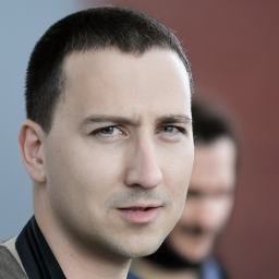
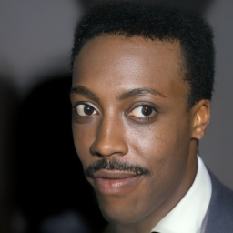
(c) Our

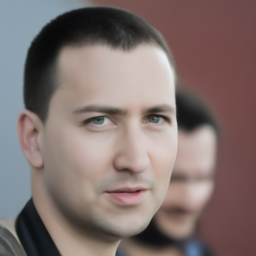
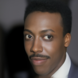
(d) DDRM

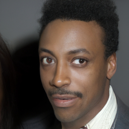
(e) DPS

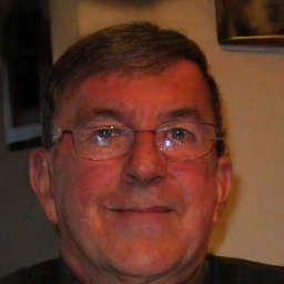
(f) $\Pi$GDM

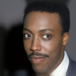
(g) DMPS

Experimental Procedure: For the super-resolution (SR) task, the input images are the downscaled versions of the ground truth high-resolution images, typically using a bicubic downsampling technique. This downscaling process simulates the loss of detail that is commonly experienced in real-world imaging scenarios. The models are then trained to reconstruct the high-resolution images from the low-resolution inputs.

In the denoising task, the images are corrupted with Gaussian noise at a higher level of intensity (with a standard deviation of $\sigma=0.5$) to test the models’ ability to remove noise and restore the original image quality. The models are evaluated on their performance to recover a clean image while preserving details.

For the inpainting task, portions of the images are masked out, either by a box shape or a text image, to simulate missing or damaged regions. The models are trained to inpaint these missing areas with plausible content that matches the surrounding context. For the SR and inpainting tasks, Gaussian noise is also added with a mean of zero and a standard deviation of $\sigma=0.05$.

Figure 3: The results for denoising. All measurements are with Gaussian noise $\sigma=0.5$, where GT stands for Ground Truth.

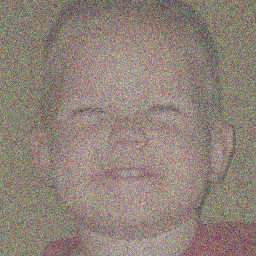
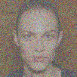
(a) Input

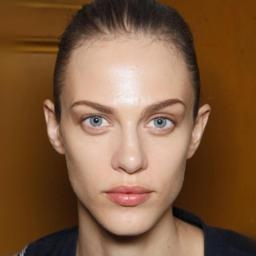
(b) GT

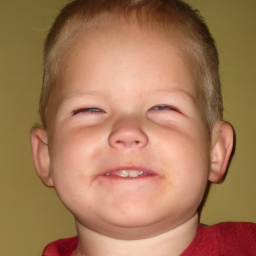
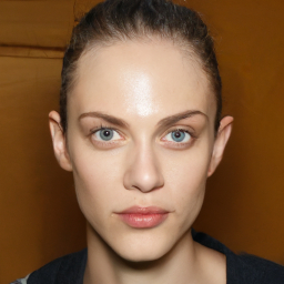
(c) Our

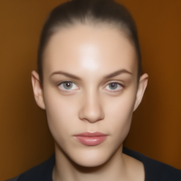
(d) DDRM

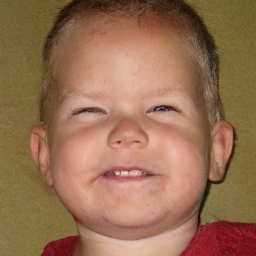
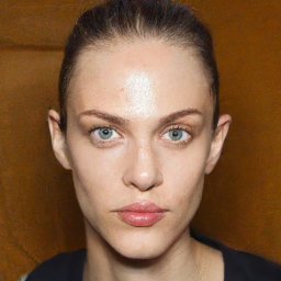
(e) DPS

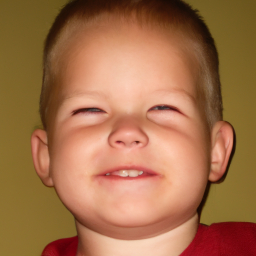
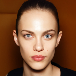
(f) $\Pi$GDM

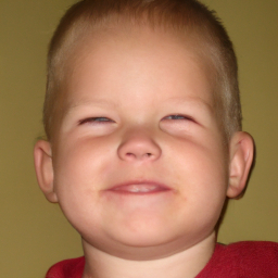
(g) DMPS

Datasets Quality and Pre-trained Models: We use the pretrained models from the Denoising Diffusion Probabilistic Models (DDPM), which were originally trained on the FFHQ 256x256-1k dataset. These pretrained models are directly used for testing without further fine-tuning for specific tasks. To evaluate the performance of our method, we conduct experiments on FFHQ 256x256-1k (the in-distribution validation set) and CelebA-HQ 256x256-1k (out-of-distribution (OOD) validation set).

Table 1: Quantitative comparisons (PSNR (dB), LPIPS) of different methods for the SR and Denoising tasks on the FFHQ 256$\times$256-1k validation dataset and the OOD CelebA-HQ 256$\times$256-1k validation dataset, respectively. The pre-trained model is the same for our proposed method, DDRM, DPS, $\Pi$GDM, DMPS, which is trained on FFHQ dataset.

			SR($\times$4)			DENOISE
Dataset	Method		PSNR↑	LPIPS↓		PSNR↑	LPIPS↓
FFHQ	ours		30.63	0.2347		30.24	0.2344
	DDRM		29.25	0.3087		27.87	0.3048
	DPS		26.68	0.2717		29.16	0.2574
	$\Pi$GDM		28.69	0.2408		24.64	0.2688
	DMPS		27.23	0.2533		28.69	0.2419
CelebA	ours		31.85	0.2355		31.48	0.2243
	DDRM		30.12	0.2614		30.46	0.2332
	DPS		24.62	0.3071		29.63	0.2969
	$\Pi$GDM		30.57	0.2509		23.97	0.2510
	DMPS		26.70	0.2603		28.96	0.3060

Table 2: Quantitative comparison (PSNR (dB), LPIPS) of different methods for different inpainting tasks on the FFHQ 256$\times$256-1k validation dataset and the OOD CelebA-HQ 256$\times$256-1k validation dataset. The pre-trained model is the same for our proposed method, DDRM, DPS, $\Pi$GDM, DMPS, which is trained on FFHQ dataset.

			BOX			LOLCAT			LOREM
DATASET	METHOD		PSNR↑	LPIPS↓		PSNR↑	LPIPS↓		PSNR↑	LPIPS↓
FFHQ	ours		30.06	0.2768		31.24	0.2587		31.31	0.2097
	DDRM		29.88	0.2373		30.50	0.2458		31.27	0.2222
	DPS		23.78	0.2455		30.46	0.2367		28.57	0.2124
	$\Pi$GDM		20.46	0.2312		17.55	0.3416		22.69	0.3088
	DMPS		24.37	0.2338		22.97	0.2429		27.65	0.2132
CelebA	ours		31.10	0.2071		33.42	0.2400		32.93	0.2077
	DDRM		29.88	0.2373		31.23	0.2403		32.07	0.2085
	DPS		23.20	0.2215		29.63	0.2421		29.06	0.2185
	$\Pi$GDM		21.09	0.2287		15.59	0.4110		21.59	0.3369
	DMPS		23.19	0.2106		18.97	0.3031		28.20	0.2187

Figure 4: The results for Inpainting (Box).

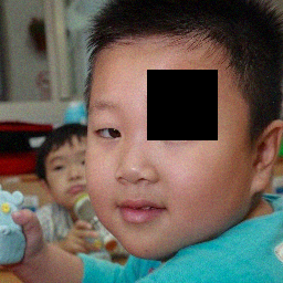
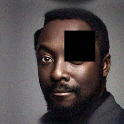
(a) Input

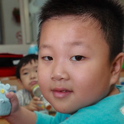
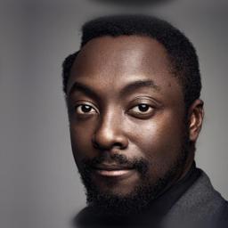
(b) GT

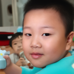
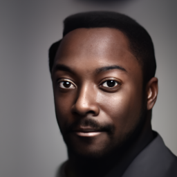
(c) Our

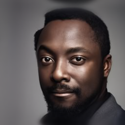
(d) DDRM

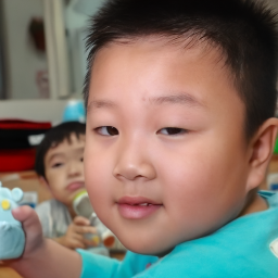
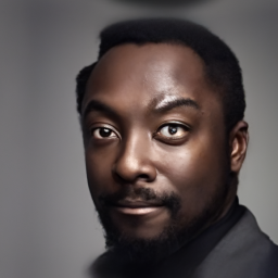
(e) DPS

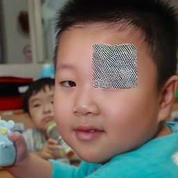
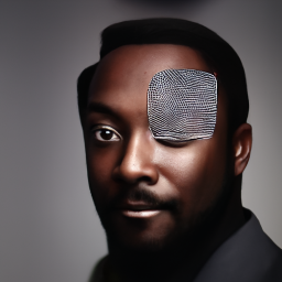
(f) $\Pi$GDM

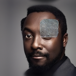
(g) DMPS

Figure 5: The results for Inpainting (Lolcat) and Inpainting (Lorem), which are presented in the first and second rows, respectively.

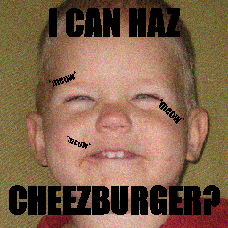
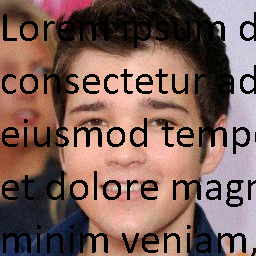
(a) Input

(b) GT

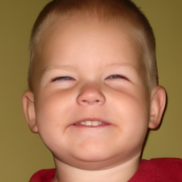
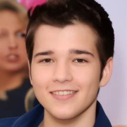
(c) Our

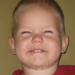
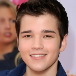
(d) DDRM

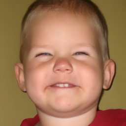
(e) DPS

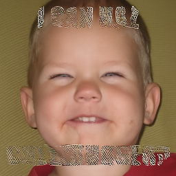
(f) $\Pi$GDM

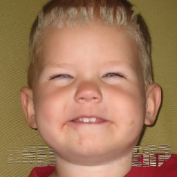
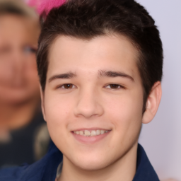
(g) DMPS

Contrastive Methods and Evaluation Metrics: We conduct comparisons with four methods: DDRM, DPS, $\Pi$GDM, and DMPS, all of which are based on the DDPM (Denoising Diffusion Probabilistic Model) framework but differ in the way they sample from the posterior distribution. To ensure a fair and objective comparison, we use the same evaluation metrics for all the different diffusion-based methods.

The performance of the models is assessed using standard distortion metrics such as Peak Signal-to-Noise Ratio (PSNR) and perceptual metrics like Learned Perceptual Image Patch Similarity (LPIPS). PSNR measures the difference between the reconstructed and original images, while LPIPS evaluates their perceptual similarity using a deep feature network. Both metrics assess the fidelity of the reconstructed images to the ground truth, as well as their visual quality, but they may have different preferences or trade-offs.

4.2 Super Resolution

For the super-resolution task, the original high-resolution images undergo bicubic downsampling to create low-resolution versions. These low-resolution images serve as the input measurements to the super-resolution model, which then generates the $4\times$ super-resolved output image.

For our proposed method, we fix the parameters $q_{1}=2$, $q_{2}=10$, and set $\eta=200$. It is clearly demonstrated in Table 1 for SR that our model outperforms other state-of-the-art diffusion models by a large margin in both in-distribution (FFHQ) and out-of-distribution (CelebA) experiments. Our method achieves the highest PSNR (30.63 and 31.85) and the lowest LPIPS (0.2347 and 0.2355) score, highlighting its outstanding quality and impressive performance.

In Figure 2, we show some examples of super-resolution on two datasets and compare them with other models. From these illustrations in Figure 2, we can see that the images generated by DDRM are too smooth and lose a lot of details. The other models also handle the special features very unnaturally, and the generated images are far from the truth and reality, particularly evident in the portrayal of the eyes. Specifically, the depiction of the eyes in the generated images lacks realism and fails to capture the intricate details that make them lifelike. Additionally, the models struggle to accurately represent eyeglasses, resulting in subpar visual representation. However, our model overcomes these challenges and achieves better results in these aspects, providing more realistic and detailed images.

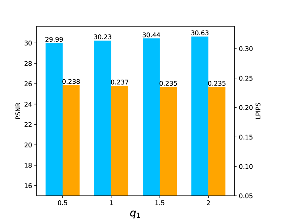
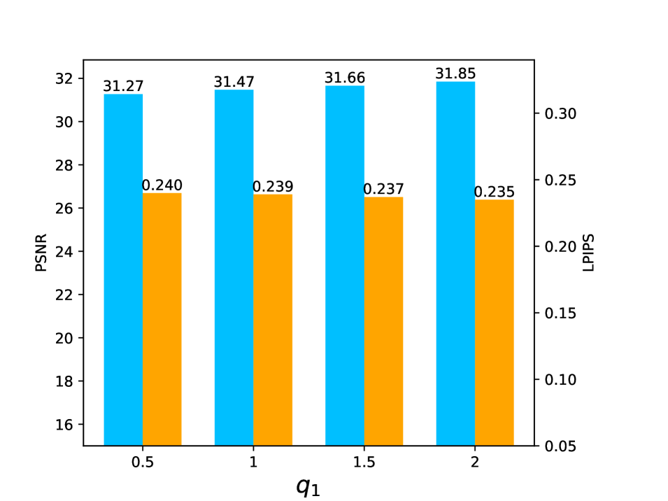
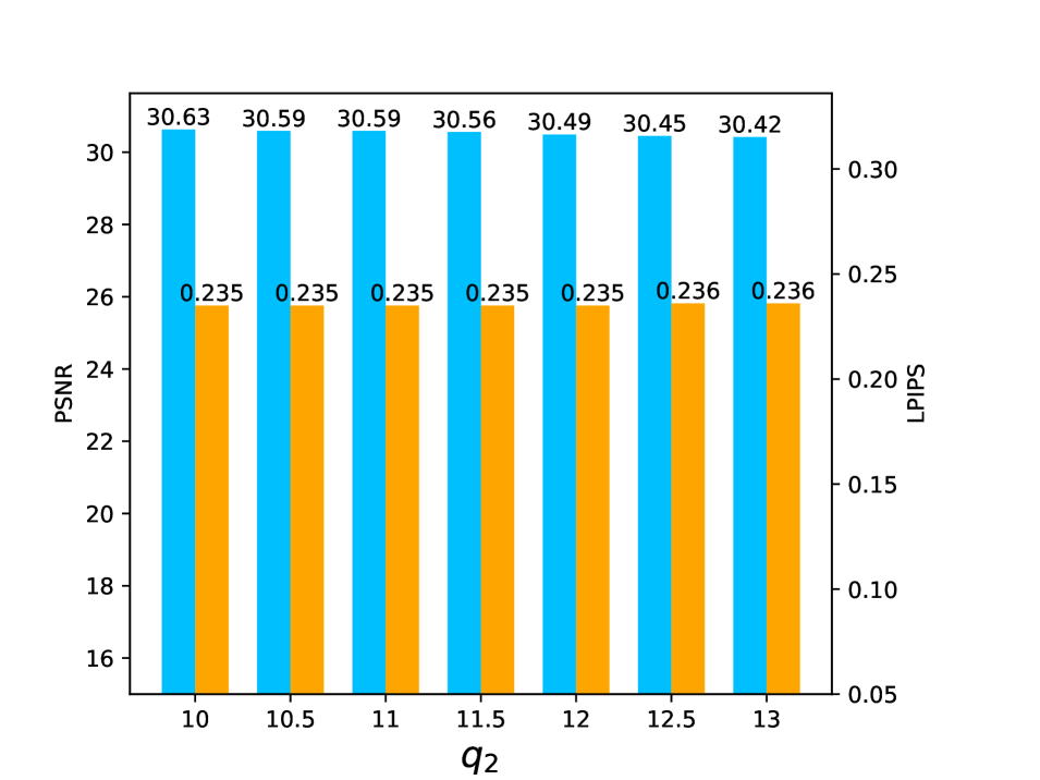
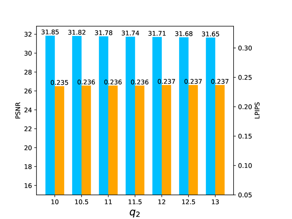
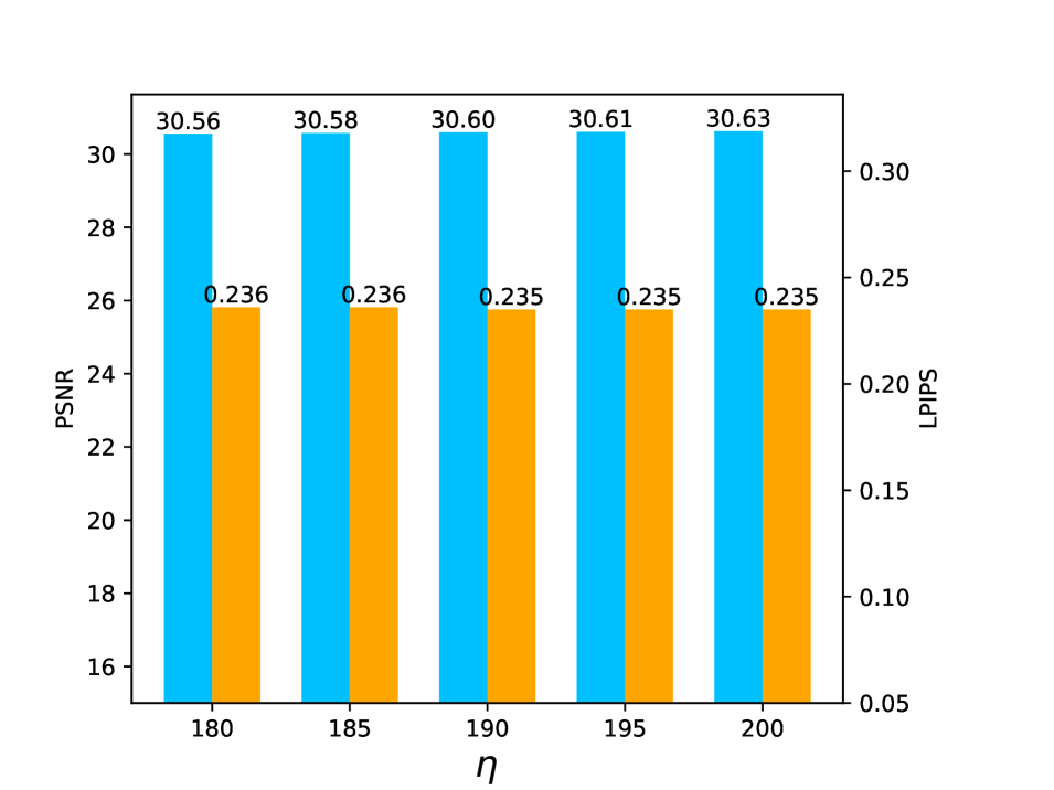
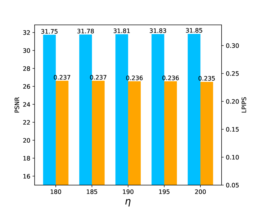
Figure 6: The robustness analysis results for Super-resolution on the FFHQ 256×256-1k (first row) and the OOD CelebA-HQ 256×256-1k (second row) validation sets with different parameters. Columns 1-3 are the plots of PSNR and LPIPS values versus the changes of parameters $q_{1}$, $q_{2}$, and $\eta$, with the other two fixed.

It also demonstrates adaptability of the model to CelebA dataset, although the pretrained models are originally trained on FFHQ 256x256-1k dataset.

4.3 Denoising

In denoising tasks, Gaussian noise is typically added to the image to simulate image degradation in the real world. The intensity of the noise determines the degree to which the noise affects the image, with higher values indicating higher noise and worse image quality degradation. To evaluate the model’s performance in denoising tasks, we deliberately introduce high-intensity ($\sigma$=0.5) Gaussian noise to corrupt the images. The goal is to test the model’s ability to remove noise while preserving the original image’s clarity and fine details. We set the parameters $q_{1}=12,q_{2}=22,\eta=2.2$ and $q_{1}=10,q_{2}=22,\eta=2.2$ for the FFHQ 256$\times$256-1k and the OOD CelebA-HQ 256$\times$256-1k validation sets, respectively. To assess the effectiveness and performance of the model in denoising tasks, we adopt two evaluation metrics, PSNR and LPIPS. Similar to the case of super-resolution, our model shows an impressive performance in the denoising task (see the right part in Table 1).

In Figure 3, we show some examples of denoising on two datasets and compare them with other models. Analyzing the examples provided, it becomes evident that the images generated by DDRM and $\Pi$GDM exhibit an overly smooth appearance, resulting in a loss of fine details. Additionally, $\Pi$GDM tends to produce images that appear overly vibrant with higher color saturation. On the other hand, DPS generates images that are extremely sharp and may still retain some noise, resulting in an exaggerated emphasis on details and potential imperfections in the generated images. Moreover, there are instances where DPS introduces additional details on the faces, resembling noise artifacts. Moving on to DMPS, specific examples further illustrate its strengths and weaknesses. For instance, in the first image, the teeth details of the person are missing, and in the second image, an imperfection such as a mole appears on the right side of the person’s nose, which does not exist in the original image. Overall, our model outperforms these methods in terms of preserving fine details and achieving more realistic results.

4.4 Inpainting

We evaluate the proposed approach against baselines diffusion models on three types of image inpainting tasks: Inpainting (Box), Inpainting (Lolcat), and Inpainting (Lorem). We use the parameters $q_{1}=12$, $q_{2}=23$, and $\eta=3$ for Inpainting (Lolcat), Inpainting (Lorem) and the parameters $q_{1}=10$, $q_{2}=24$, and $\eta=4$ for Inpainting (Box). Table 2 presents the quantitative results of our model and other methods on the image inpainting tasks, using two metrics: PSNR and LPIPS.

In this set of experiments, our method achieves the best performance in PSNR across almost all tasks, while exhibiting relatively lower performance in LPIPS for some tasks (see Table 2). However, on average, our model still demonstrates excellent quality compared to other models, as illustrated in Figure 4 and Figure 5, which showcase qualitative examples of the inpainted images generated by different methods.

From the examples presented, it is evident that DDRM handles the special features very unnaturally. The generated images exhibit highly unnatural depiction of the person’s eyes, and in some cases, there are noticeable traces of text shapes appearing on the person’s chin, where was originally covered by text. As a result, the generated images produced by DDRM are quite far from real images and do not reflect reality accurately. $\Pi$GDM is only able to remove lighter masks and completely fail to remove masks that covered a significant amount of relevant information. DMPS performs somewhat better than $\Pi$GDM, as it is able to partially remove some masks, but still left noticeable traces in the generated images. DPS is unable to accurately depict images with sharp edges, as seen in the first image of the Inpainting (Box) task where the edge of the person’s forehead, covered by the mask, appears twisted. In the Inpainting (Lolcat) and Inpainting (Lorem) tasks, the teeth of the person in the first image and the line of the person’s clothing in the second image are significantly distorted from the real images. Given these observations, it is clear that our model achieve better performance overall in the inpainting task compared to the other models.

4.5 Parameter Selection

In order to select the most suitable parameters of our proposed method, extensive experiments are conducted on the validation set for all tasks. The primary objective of these experiments is to identify the optimal parameter combinations. Numerical results for the super-resolution tasks are presented in Figure 6. We have very similar numerical results for denoising and inpainting. We omit the results to save space. Interestingly, our finding reveals that the changes in these parameters had minimal impact on the PSNR and LPIPS values, indicating the robustness of our model. This observation underscores the ability of our model to consistently deliver high-quality results across different parameter settings. Such robustness is a highly desirable characteristic as it ensures the model’s performance remains stable and reliable even when faced with variations in inputs or parameter values.

5 Conclusion

In this paper, we propose a novel, problem-agnostic diffusion model called the MAP-based Guided Term Estimation method for inverse problems. First, we divide the conditional score function into two terms according to Bayes’ rule: the unconditional score function and the guided term. We design the MAP-based Guided Term Estimation method, while the unconditional score function is approximated by an existing score network. Numerical experiments validate the efficacy of our proposed method on a variety of linear inverse problems, such as super-resolution, inpainting, and denoising. Through extensive evaluations, we have demonstrated that our method achieves comparable performance to state-of-the-art diffusion models, including DDRM, DPS, $\Pi$GDM and DMPS.

With further advancements and refinements, this approach has the potential to contribute to the development of more effective and robust solutions in various fields.

Limitations & Future Works: While this paper makes valuable contributions, there are some limitations that suggest future research directions. (1) Our approach relies on the assumption that the space of clean natural images is inherently smooth, which may result in the loss of certain features. (2) The numerical experiments in this work focus solely on linear inverse problems and do not extend to nonlinear cases.

Appendix A Derivation of the estimated value

A.1 The computation of spatial derivative $\nabla_{\mathbf{x}_{t}}\mathbf{S}_{\theta}(\mathbf{x}_{t},t)$

Note that

$$\frac{-\mathbf{S}_{\theta}(\mathbf{x}_{t},t)}{\sqrt{\zeta_{t}}}\overset{model}{\approx}\nabla_{\mathbf{x}_{t}}\log p(\mathbf{x}_{t},t)\underset{t\neq 0}{\overset{almost\ equal}{\approx}}\nabla_{\mathbf{x}_{t}}\log p(\mathbf{x}_{t},t|\mathbf{x}_{0},0)=-\frac{\mathbf{x}_{t}-\sqrt{1-\zeta_{t}}\mathbf{x}_{0}}{\zeta_{t}}.$$

Therefore,

$$\nabla_{\mathbf{x}_{t}}\mathbf{S}_{\theta}(\mathbf{x}_{t},t)=\frac{1}{\sqrt{\zeta_{t}}}I.$$ (A.1)

A.2 Time derivation $\partial_{t}\mathbf{S}_{\theta}(\mathbf{x}_{t},t)$

Next, let us compute $\partial_{t}\mathbf{S}_{\theta}(\mathbf{x}_{t},t)$. Note that $\mathbb{E}[\mathbf{x}_{0}|\mathbf{x}_{t}]=\frac{1}{\sqrt{1-\zeta_{t}}}\left(\mathbf{x}_{t}-\sqrt{\zeta_{t}}\mathbf{S}_{\theta}(\mathbf{x}_{t},t)\right)$, then

$$\mathbf{S}_{\theta}(\mathbf{x}_{t},t)=\frac{\mathbf{x}_{t}-\sqrt{1-\zeta_{t}}\mathbb{E}[\mathbf{x}_{0}|\mathbf{x}_{t}]}{\sqrt{\zeta_{t}}}.$$ (A.2)

Since $\zeta_{t}=1-e^{-\int^{t}_{0}\beta_{t}dt}$, We have the derivative of $\zeta_{t}$ about $t$ is

$$\dot{\zeta}_{t}=(1-\zeta_{t})\beta(t).$$ (A.3)

Assume $\partial_{t}\mathbb{E}[\mathbf{x}_{0}|\mathbf{x}_{t}]=0$, we get from (A.2) and (A.3)

$$\partial_{t}\mathbf{S}_{\theta}(\mathbf{x}_{t},t)=\partial_{t}\frac{\mathbf{x}_{t}-\sqrt{1-\zeta_{t}}\mathbb{E}[\mathbf{x}_{0}|\mathbf{x}_{t}]}{\sqrt{\zeta_{t}}}$$

$$\approx \frac{1}{\sqrt{\zeta_{t}}}\left(\frac{1}{2}\dot{\zeta}_{t}(1-\zeta_{t})^{-1/2}\mathbb{E}[\mathbf{x}_{0}|\mathbf{x}_{t}]\right)+(\mathbf{x}_{t}-\sqrt{1-\zeta_{t}}\mathbb{E}[\mathbf{x}_{0}|\mathbf{x}_{t}])\left(-\frac{1}{2}\dot{\zeta}_{t}\zeta_{t}^{-3/2}\right)$$

$$= \frac{\dot{\zeta}_{t}}{2\zeta_{t}^{3/2}}\left(\frac{\zeta_{t}}{\sqrt{1-\zeta_{t}}\mathbb{E}[\mathbf{x}_{0}|\mathbf{x}_{t}]}-(\mathbf{x}_{t}-\sqrt{1-\zeta_{t}}\mathbb{E}[\mathbf{x}_{0}|\mathbf{x}_{t}])\right)=\frac{\dot{\zeta}_{t}}{2\zeta_{t}^{3/2}}\left(-\mathbf{x}_{t}+\frac{1}{\sqrt{1-\zeta_{t}}}\mathbb{E}[\mathbf{x}_{0}|\mathbf{x}_{t}]\right)$$

$$= \frac{\dot{\zeta}_{t}}{2\zeta_{t}^{3/2}}\left(-\mathbf{x}_{t}+\frac{1}{\sqrt{1-\zeta_{t}}}\frac{1}{\sqrt{1-\zeta_{t}}}\left(\mathbf{x}_{t}-\sqrt{\zeta_{t}}\mathbf{S}_{\theta}(\mathbf{x}_{t},t)\right)\right)$$

$$= \frac{\dot{\zeta}_{t}}{2\zeta_{t}^{3/2}}\left(\left(-1+\frac{1}{1-\zeta_{t}}\right)\mathbf{x}_{t}-\frac{\sqrt{\zeta_{t}}}{1-\zeta_{t}}\mathbf{S}_{\theta}(\mathbf{x}_{t},t)\right)$$

$$= \frac{1}{2\zeta_{t}^{3/2}}\frac{\dot{\zeta}_{t}}{1-\zeta_{t}}\left(\zeta_{t}\mathbf{x}_{t}-\sqrt{\zeta_{t}}\mathbf{S}_{\theta}(\mathbf{x}_{t},t)\right)$$

$$= \frac{1}{2\zeta_{t}^{3/2}}\beta(t)\left(\zeta_{t}\mathbf{x}_{t}-\sqrt{\zeta_{t}}\mathbf{S}_{\theta}(\mathbf{x}_{t},t)\right)=\frac{\beta(t)}{2\sqrt{\zeta_{t}}}\left(\mathbf{x}_{t}-\frac{\mathbf{S}_{\theta}(\mathbf{x}_{t},t)}{\sqrt{\zeta_{t}}}\right).$$

Proof of Theorem 3.1.

We consider the Taylor expansion:

$$\mathbf{S}_{\theta}(\mathbf{x}_{0},0)=\mathbf{S}_{\theta}(\mathbf{x}_{t},t) + (0-t)\partial_{t}\mathbf{S}_{\theta}(\mathbf{x}_{t},t)$$ (A.4)

$$+ (\mathbf{x}_{0}-\mathbf{x}_{t})^{\top}\nabla_{\mathbf{x}_{t}}\mathbf{S}_{\theta}(\mathbf{x}_{t},t)+o(\|\mathbf{x}_{t}-\mathbf{x}_{0}\|+|t|),$$

Since $\bar{\alpha}_{t}=1-\zeta_{t}$, using the results in Subsections A.1 and A.2, we have

$$\hat{\mathbf{x}} =\frac{\mathbf{x}_{t}}{\sqrt{1-\zeta_{t}}}+\frac{\zeta_{t}}{1-\zeta_{t}}\nabla_{\mathbf{\hat{x}}}\log p(\mathbf{\hat{x}})$$

$$\approx\frac{\mathbf{x}_{t}}{\sqrt{\overline{\alpha_{t}}}}-\frac{\sqrt{1-\overline{\alpha_{t}}}}{\overline{\alpha_{t}}}\mathbf{S}_{\theta}(\mathbf{\hat{x}},0)$$

$$=\frac{\mathbf{x}_{t}}{\sqrt{\overline{\alpha_{t}}}}-\frac{\sqrt{1-\overline{\alpha_{t}}}}{\overline{\alpha_{t}}}(\mathbf{S}_{\theta}(\mathbf{x}_{t},t)+(0-t)\partial_{t}\mathbf{S}_{\theta}(\mathbf{x}_{t},t)+\nabla_{\mathbf{x}_{t}}\mathbf{S}_{\theta}(\mathbf{x}_{t},t)^{\top}(\mathbf{\hat{x}}-\mathbf{x}_{t})+o(\|\mathbf{x}_{t}-\mathbf{x}_{0}\|+|t|))$$

$$=\frac{\mathbf{x}_{t}}{\sqrt{\overline{\alpha_{t}}}}-\frac{\sqrt{1-\overline{\alpha_{t}}}}{\overline{\alpha_{t}}}\left(\mathbf{S}_{\theta}(\mathbf{x}_{t},t)-t\frac{\beta_{t}}{2\sqrt{1-\overline{\alpha_{t}}}}\left(x_{t}-\frac{\mathbf{S}_{\theta}(\mathbf{x}_{t},t)}{\sqrt{1-\overline{\alpha_{t}}}}\right)+\frac{\mathbf{\hat{x}}-\mathbf{x}_{t}}{\sqrt{1-\overline{\alpha_{t}}}}\right)+o(\|\mathbf{x}_{t}-\mathbf{x}_{0}\|+|t|)$$

$$=\frac{\mathbf{x}_{t}}{\sqrt{\overline{\alpha_{t}}}}-\frac{\sqrt{1-\overline{\alpha_{t}}}}{\overline{\alpha_{t}}}\mathbf{S}_{\theta}(\mathbf{x}_{t},t)+q_{1}\left(t\mathbf{x}_{t}\frac{\beta_{t}}{2\overline{\alpha_{t}}}-t\frac{\beta_{t}\mathbf{S}_{\theta}(\mathbf{x}_{t},t)}{2\overline{\alpha_{t}}\sqrt{1-\overline{\alpha_{t}}}}\right)-q_{2}\frac{\mathbf{\hat{x}}-\mathbf{x}_{t}}{\overline{\alpha_{t}}}$$

$$=\frac{\mathbf{x}_{t}}{\sqrt{\overline{\alpha_{t}}}}-\frac{\sqrt{1-\overline{\alpha_{t}}}}{\overline{\alpha_{t}}}\mathbf{S}_{\theta}(\mathbf{x}_{t},t)+q_{1}t\mathbf{x}_{t}\frac{\beta_{t}}{2\overline{\alpha_{t}}}-q_{1}t\frac{\beta_{t}\mathbf{S}_{\theta}(\mathbf{x}_{t},t)}{2\overline{\alpha_{t}}\sqrt{1-\overline{\alpha_{t}}}}-q_{2}\frac{\mathbf{\hat{x}}-\mathbf{x}_{t}}{\overline{\alpha_{t}}}$$

$$=\frac{\mathbf{x}_{t}}{\sqrt{\overline{\alpha_{t}}}}-\frac{\sqrt{1-\overline{\alpha_{t}}}}{\overline{\alpha_{t}}}\mathbf{S}_{\theta}(\mathbf{x}_{t},t)+\frac{q_{1}t\beta_{t}}{2\overline{\alpha_{t}}}\mathbf{x}_{t}-\frac{q_{1}t\beta_{t}\mathbf{S}_{\theta}(\mathbf{x}_{t},t)}{2\overline{\alpha_{t}}\sqrt{1-\overline{\alpha_{t}}}}-\frac{q_{2}}{\overline{\alpha_{t}}}(\mathbf{\hat{x}}-\mathbf{x}_{t}),$$ (A.5)

For the fourth equality, we express the higher-order term $o(\|\mathbf{x}_{t}-\mathbf{x}_{0}\|+|t|)$ in terms of the first-order term by introducing parameters $q_{1}$ and $q_{2}$. When $(\mathbf{x}_{t},t)$ is far from $(\mathbf{x}_{0},0)$, the parameters $(q_{1},q_{2})$ may be large, and conversely. The final result of $\hat{\mathbf{x}}$ is:

$$\hat{\mathbf{x}} = \frac{(\sqrt{\overline{\alpha_{t}}}+\frac{q_{1}t\beta_{t}}{2}+q_{2})\mathbf{x}_{t}-(\sqrt{1-\overline{\alpha_{t}}}+\frac{q_{1}t\beta_{t}}{2\sqrt{1-\overline{\alpha_{t}}}})\mathbf{S}_{\theta}(\mathbf{x}_{t},t)}{(\overline{\alpha_{t}}+q_{2})}.$$

∎

Remark A.1.

It is worth noting that we use a strategy very similar to that of Newton’s method in optimization in the third line of (A.2).

References

- [1] J. Choi, S. Kim, Y. Jeong, Y. Gwon, S. Yoon, Ilvr: Conditioning method for denoising diffusion probabilistic models, in: 2021 IEEE/CVF International Conference on Computer Vision (ICCV), IEEE, 2021, pp. 14347–14356.
- [2] Y. Song, J. Sohl-Dickstein, D. P. Kingma, A. Kumar, S. Ermon, B. Poole, Score-based generative modeling through stochastic differential equations, in: International Conference on Learning Representations, 2021.
- [3] Y. Song, L. Shen, L. Xing, S. Ermon, Solving inverse problems in medical imaging with score-based generative models, in: International Conference on Learning Representations, 2021.
- [4] H. Chung, B. Sim, D. Ryu, J. C. Ye, Improving diffusion models for inverse problems using manifold constraints, Advances in Neural Information Processing Systems 35 (2022) 25683–25696.
- [5] B. Kawar, M. Elad, S. Ermon, J. Song, Denoising diffusion restoration models, Advances in Neural Information Processing Systems 35 (2022) 23593–23606.
- [6] H. Chung, J. Kim, M. T. Mccann, M. L. Klasky, J. C. Ye, Diffusion posterior sampling for general noisy inverse problems, in: The Eleventh International Conference on Learning Representations, 2023.
- [7] J. Song, A. Vahdat, M. Mardani, J. Kautz, Pseudoinverse-guided diffusion models for inverse problems, in: International Conference on Learning Representations, 2022.
- [8] X. Meng, Y. Kabashima, Diffusion model based posterior sampling for noisy linear inverse problems, Proceedings of Machine Learning Research (2024).
- [9] J. Sohl-Dickstein, E. Weiss, N. Maheswaranathan, S. Ganguli, Deep unsupervised learning using nonequilibrium thermodynamics, in: International conference on machine learning, PMLR, 2015, pp. 2256–2265.
- [10] J. Ho, A. Jain, P. Abbeel, Denoising diffusion probabilistic models, Advances in neural information processing systems 33 (2020) 6840–6851.
- [11] Z. Kadkhodaie, E. Simoncelli, Stochastic solutions for linear inverse problems using the prior implicit in a denoiser, Advances in Neural Information Processing Systems 34 (2021) 13242–13254.
- [12] A. Jalal, M. Arvinte, G. Daras, E. Price, A. G. Dimakis, J. Tamir, Robust compressed sensing mri with deep generative priors, Advances in Neural Information Processing Systems 34 (2021) 14938–14954.
- [13] A. Graikos, N. Malkin, N. Jojic, D. Samaras, Diffusion models as plug-and-play priors, Advances in Neural Information Processing Systems 35 (2022) 14715–14728.
- [14] H. Chung, J. Kim, S. Kim, J. C. Ye, Parallel diffusion models of operator and image for blind inverse problems, in: Proceedings of the IEEE/CVF Conference on Computer Vision and Pattern Recognition, 2023, pp. 6059–6069.
- [15] Y. He, N. Murata, C.-H. Lai, Y. Takida, T. Uesaka, D. Kim, W.-H. Liao, Y. Mitsufuji, J. Z. Kolter, R. Salakhutdinov, et al., Manifold preserving guided diffusion, in: The Twelfth International Conference on Learning Representations, 2024.
- [16] A. Bora, A. Jalal, E. Price, A. G. Dimakis, Compressed sensing using generative models, in: International conference on machine learning, PMLR, 2017, pp. 537–546.
- [17] J. Dean, G. Daras, A. Dimakis, Intermediate layer optimization for inverse problems using deep generative models, in: NeurIPS 2020 Workshop on Deep Learning and Inverse Problems, 2020.
- [18] G. Ongie, A. Jalal, C. A. Metzler, R. G. Baraniuk, A. G. Dimakis, R. Willett, Deep learning techniques for inverse problems in imaging, IEEE Journal on Selected Areas in Information Theory 1 (1) (2020) 39–56.
- [19] S. Arjomand Bigdeli, M. Zwicker, P. Favaro, M. Jin, Deep mean-shift priors for image restoration, Advances in Neural Information Processing Systems 30 (2017).
- [20] L. I. Rudin, S. Osher, E. Fatemi, Nonlinear total variation based noise removal algorithms, Physica D: nonlinear phenomena 60 (1-4) (1992) 259–268.
- [21] R. Fergus, B. Singh, A. Hertzmann, S. T. Roweis, W. T. Freeman, Removing camera shake from a single photograph, ACM Transactions on Graphics 25 (3) (2006) 787–794.
- [22] H. Tachibana, M. Go, M. Inahara, Y. Katayama, Y. Watanabe, Quasi-taylor samplers for diffusion generative models based on ideal derivatives, arXiv preprint arXiv:2112.13339 (2021).
- [23] P. Vincent, A connection between score matching and denoising autoencoders, Neural computation 23 (7) (2011) 1661–1674.