Abstract

Long-term time series forecasting is essential in areas like finance and weather prediction. Besides traditional methods that operate in the time domain, many recent models transform time series data into the frequency domain to better capture complex patterns. However, these methods often use filtering techniques to remove certain frequency signals as noise, which may unintentionally discard important information and reduce prediction accuracy. To address this, we propose the Frequency Decomposition Mixture of Experts (FreqMoE) model, which dynamically decomposes time series data into frequency bands, each processed by a specialized expert. A gating mechanism adjusts the importance of each output of expert based on frequency characteristics, and the aggregated results are fed into a prediction module that iteratively refines the forecast using residual connections. Our experiments demonstrate that FreqMoE outperforms state-of-the-art models, achieving the best performance on 51 out of 70 metrics across all tested datasets, while significantly reducing the number of required parameters to under 50k, providing notable efficiency advantages.

1 INTRODUCTION

The task of time series forecasting aims to predict the future based on known past time series data and has broad applications in fields such as finance(Ariyo et al.,, 2014), weather forecasting(Zhu et al.,, 2023), energy consumption(Zufferey et al.,, 2017), and healthcare management(Zeroual et al.,, 2020).Traditional statistical methods, such as the Autoregressive Integrated Moving Average (Nelson,, 1998) and exponential smoothing(Gardner Jr,, 1985), were once widely used for time series analysis. However, these methods often perform poorly when dealing with nonlinear, non-stationary, and multi-sequence real-world datasets(Li and Zong,, 2012).

In recent years, to address the limitations of traditional models in capturing complex patterns and dynamic features in time series, numerous studies have proposed sophisticated models and methodologies based on MLP(Das et al.,, 2024; Wang et al.,, 2024; Zeng et al.,, 2022) and transformer architectures(Zhou et al.,, 2021; Zhou et al., 2022b, ; Wu et al.,, 2022; Nie et al.,, 2023), which have achieved significant improvements over traditional methods. Despite their success, these models primarily operate in the time domain and may not fully leverage the frequency characteristics of time series data, such as seasonality and cyclic patterns(Box et al.,, 2015).

As a result, more and more models are shifting towards frequency domain analysis(Liu et al.,, 2023; Zhou et al., 2022b, ; Wu et al.,, 2023). By utilizing techniques such as Fast Fourier Transform (FFT), time series data can be decomposed into their respective frequency components, making it easier to analyze periodic behaviors and trends that are difficult to observe in the time domain. Although some models, such FITS(Xu et al.,, 2024), have employed frequency domain analysis for time series forecasting, but it relies on fixed filtering techniques. We believe that applying fixed filters indiscriminately across different datasets is unreasonable. Instead, the weights for different frequency bands should be dynamically assigned based on the frequency characteristics of the data to prevent the loss of important information and improve forecasting accuracy.

In this paper, we propose a novel Frequency Decomposition Mixture-of-Experts model. Our approach leverages the frequency domain representation of time series data by decomposing the input into different frequency bands, with each expert network focusing on a specific frequency range. A gating network dynamically assigns weights to each expert based on the frequency magnitude, enabling a data-driven combination of expert outputs. The aggregated output is then fed into a prediction architecture consisting of multiple deep residual blocks, achieving end-to-end time series forecasting.

Our primary contributions include:

1. We introduce a frequency decomposition MoE module where each expert network focuses on a specific frequency range of the input data. This specialization enables the model to capture intricate patterns associated with different frequency components.

2. We develop a gated network that operates on the frequency magnitude spectrum, dynamically weighting the contribution of each expert according to the frequency properties of the input. This mechanism allows the model to more fully utilize all the information and extract the dominant frequency patterns.

3. A prediction structure combining the frequency upsampling technique with the stacked depth residual module is proposed, which together with the frequency decomposition MoE module forms FreqMoE, a powerful forecast model, achieves consistent state-of-the-art performance across multiple domains.

2 RELATED WORK AND MOTIVATION

2.1 Long-horizon Time-series Forecasting Models

Transformer-based models were originally developed for natural language processing(Vaswani,, 2017), but have been used for long-term time series forecasting due to their ability to capture long-term dependencies through a self-attention mechanism. For example, the earliest Transformer-based model, Informer(Zhou et al.,, 2021), solves the problem of squared time complexity growth by using the self-attention extraction mechanism, as well as Autoformer(Wu et al.,, 2022), which uses autocorrelation decomposition, and FEDformer(Zhou et al., 2022b, ), which employs frequency augmentation and sequence decomposition, and PatchTST(Nie et al.,, 2023), which is the most recent model that introduces the idea of patch These models have been shown to have good results in complex time series prediction.

Despite the success of transformer-based models in long-term time series forecasting (LTSF), Zeng et al., (2022), still gave doubts about the effectiveness of transformer-based models and proposed a Dlinear model consisting of only one simple linear layer, which proved the simplicity and efficiency of MLP-based models. Similarly, the subsequently proposed TimeMixer model(Wang et al.,, 2024) also uses only multiple MLP layers combined with a downsampling mechanism to capture temporal dependencies, showing that a well-designed MLP model can match or exceed transformer in prediction tasks.

2.2 Motivation

With the continuous development of the field, some models are gradually shifting from time-domain prediction to frequency-domain prediction, such as FEDformer use frequency domain enhancement module combined with transformer for prediction(Zhou et al., 2022b, ), TimesNet decompose time series into multiple periods by Fourier tansforms (Wu et al.,, 2023), and FITS predict with complex linear layer after apply a low-pass filter(Xu et al.,, 2024). However, many frequency-domain prediction models now treat high-frequency components as noise that should be discarded(Xu et al.,, 2024; Zhou et al., 2022a, ), but directly recognizing high-frequency components as noise in the absence of a prior knowledge may result in the loss of important information, thus reducing the prediction accuracy(Zhang et al.,, 2024).

To address this problem, we believe that the fixed frequency components in the original sequence should not be directly deleted. Instead, the weights of each frequency should be dynamically adjusted according to the data, and different frequencies should be weighted and combined(Zhang et al.,, 2024). This can make full use of all the information and accurately extract the key frequency patterns, thus realizing more efficient prediction. Inspired by the stackable residual architecture(Oreshkin et al.,, 2020), we argue that we can exploit the properties of frequency domain signals by upsampling the sequence while reconstructing the backtracking window and making predictions. This allows the model to be iteratively optimized based on the residuals of the backtracking sequence, progressively capturing complex patterns at different frequencies.

3 PRELIMINARIES

3.1 Problem Definition

Time series forecasting aims to predict future values of a sequence based on historical observations. Formally, let $X\in\mathbb{R}^{c\times s}$ represent the input sequence, where $c$ is the number of channels or features, and $s$ denotes the number of historical time steps. The goal is to learn a mapping function $f$ such that $f(X)=Y$, where $Y\in\mathbb{R}^{c\times p}$ is the predicted sequence of future values over $p$ time steps. This mapping should minimize a predefined loss function $\text{loss}(Y,\hat{Y})$, with $\hat{Y}$ being the ground truth future values.

Generally, the forecasting performance of the model is typically evaluated using the mean squared error (MSE) and the mean absolute error (MAE) as loss functions. These functions are defined as:

$$\text{MSE}=\frac{1}{n}\sum_{i=1}^{n}(Y_{i}-\hat{Y}_{i})^{2}$$ (1)

$$\text{MAE}=\frac{1}{n}\sum_{i=1}^{n}|Y_{i}-\hat{Y}_{i}|$$ (2)

3.2 Fast Fourier Transform(FFT)

The Discrete Fourier Transform (DFT) converts discrete-time signals from the time domain to the complex frequency domain, while the Fast Fourier Transform (Brigham and Morrow,, 1967) significantly accelerates the computation of the DFT through an efficient algorithm. For real-valued input signals, the Real Fast Fourier Transform (rFFT) is typically employed, transforming $N$ real input values into $N/2+1$ complex numbers, thereby effectively representing the signal in the complex frequency domain.

4 METHODOLOGY

4.1 Overview

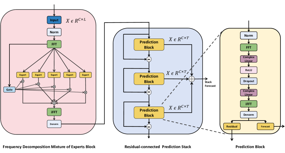
Figure 1: The complete structure of the FreqMoE model consists of a Frequency Decomposition Mixture of Experts Block, which decomposes and processes the input time series before reconstruction, and a Frequency Domain Prediction Stack, which is composed of multiple prediction blocks connected through residual connections. This model dynamically captures patterns in the sequence by leveraging the relationships and frequency characteristics across different frequency bands of the input data, enabling accurate predictions.

Motivated by exploration of frequency-domain time series forecasting and raw data filtering challenges in section 2, we introduce a deep architecture based on frequency decomposition. As illustrated in Figure 1, the architecture comprises a Frequency Decomposition Mixture of Experts module and a Frequency Domain Prediction module, the latter constructed by stacking multiple prediction blocks with residual connections. Detailed descriptions of the Frequency Decomposition Expert Network and Prediction modules are provided in Sections 4.2 and 4.3, respectively.

The input time series $\mathbf{x}\in\mathbb{R}^{B\times C\times L}$, where $B$ is the batch size, $C$ the number of channels, and $L$ the sequence length, is first normalized using mean subtraction and variance scaling, resulting in zero mean and unit variance data. Then, the normalized data is transformed into the frequency domain using the Fast Fourier Transform (FFT), resulting in

$$\mathbf{X}_{f}=\text{FFT}(\mathbf{x})\in\mathbb{C}^{B\times C\times L_{f}},$$ (3)

where $L_{f}=\frac{L}{2}+1$ is the length of the frequency domain representation. The frequency components are then divided into $N_{\text{expert}}$ disjoint regions, with each expert handling a specific frequency band. The gating network, $G(\mathbf{X}_{f})$, takes the magnitude of the frequency components, $\|\mathbf{X}_{f}\|$, as input and generates gating scores $\mathbf{g}\in\mathbb{R}^{B\times N_{\text{expert}}}$ using a softmax activation:

$$\mathbf{g}=\text{Softmax}(G(\|\mathbf{X}_{f}\|)).$$ (4)

The expert outputs are combined using frequency-domain gating scores, then transformed back to the time domain with inverse FFT and denormalized. This module enables the model to capture information from each frequency band and manage short- and long-term temporal patterns effectively.

The output from the Frequency Decomposition Mixture of Experts module is processed through several frequency domain prediction blocks, each containing two simple complex-valued linear layers. Each block upsamples the Fourier-transformed representation $\mathbf{X}_{f}$, reconstructs historical sequences, and predicts future ones. After an inverse Fourier transform and denormalization, the residual between the output and input sequences is used as input for the next block, progressively refining the predictions:

$$\mathbf{x}^{(i+1)}=\mathbf{x}^{(i)}-\hat{\mathbf{x}}^{(i)}$$ (5)

The final predicted sequence is obtained by accumulating the predictions of each block.

4.2 Frequency Decomposition Mixture of Experts Block

The Frequency Decomposition Mixture of Experts (MoE) module is one of the core components of our model. The input time series $\mathbf{X}\in\mathbb{R}^{B\times C\times L}$, where $B$ is the batch size, $C$ is the number of channels, and $L$ is the sequence length, is first transformed into the frequency domain using the Fast Fourier Transform (FFT), resulting in a frequency domain sequence $\mathbf{F}(\mathbf{X})\in\mathbb{C}^{B\times C\times F}$ of length $F=\frac{L}{2}+1$. In the frequency domain, the sequence is represented in complex form, where each component corresponds to the amplitude and phase of a specific frequency.

To fully utilize the information across all frequency bands, we introduce expert networks, with each expert responsible for processing a specific frequency range. we propose to learn the frequency band boundaries in an end-to-end manner. This allows the model to adaptively focus on the most informative frequency bands.

We parameterize the frequency band boundaries using learnable parameters $\boldsymbol{\theta}=\{\theta_{1},\theta_{2},\dots,\theta_{N-1}\}$, where $N$ is the number of experts. Each $\theta_{i}$ is a scalar value. We apply the sigmoid function to map these parameters to the interval $(0,1)$:

$$\tilde{b}_{i}=\sigma(\theta_{i})=\frac{1}{1+e^{-\theta_{i}}},\quad i=1,2,\dots,N-1.$$ (6)

To ensure that the frequency bands are non-overlapping and collectively cover the entire frequency range, we sort the normalized boundaries in ascending order, including $0$ and $1$ as the initial and final boundaries:

$$\{b_{0},b_{1},\dots,b_{N}\}=\text{Sort}\left(\{0,\tilde{b}_{1},\dots,\tilde{b}_{N-1},1\}\right),$$ (7)

where $b_{0}=0$ and $b_{N}=1$. These normalized boundaries are then mapped to actual frequency indices based on the frequency domain length $F$. For the $i$-th expert $E_{i}$, the responsible frequency range is defined as:

$$\text{Range}_{i}=\begin{cases}[f_{i-1},f_{i}),&\text{for }i=1,\dots,N-1,\\ [f_{N-1},F],&\text{for }i=N.\end{cases}$$ (8)

To ensure that each expert only processes its assigned frequency range, we construct a mask $M_{i}\in\{0,1\}^{B\times C\times F}$ for each expert $E_{i}$, defined as:

$$M_{i}(f)=\begin{cases}1,&\text{if }f\in[f_{i-1},f_{i}),\quad i=1,2,\dots,N-1,\\ 1,&\text{if }f\in[f_{N-1},F],\quad i=N,\\ 0,&\text{otherwise}.\end{cases}$$ (9)

The frequency components processed by expert $E_{i}$ are obtained by applying the mask:

$$\mathbf{F}_{i}(\mathbf{X})=M_{i}\odot\mathbf{F}(\mathbf{X}),$$ (10)

where $\odot$ denotes element-wise multiplication, and $\mathbf{F}_{i}(\mathbf{X})$ represents the frequency sub-band processed by expert $E_{i}$ after applying the mask.

After obtaining output of each expert, the gating network in the Mixture of Experts module dynamically aggregates them based on the frequency domain characteristics of input sequence. Specifically, it computes the magnitude of the frequency representation and averages it across the channel dimension to serve as input for the gating network:

$$\mathbf{G}(\mathbf{X})=\frac{1}{C}\sum_{c=1}^{C}\left|\mathbf{F}(\mathbf{X})_{c}\right|\in\mathbb{R}^{B\times F}.$$ (11)

This input $\mathbf{G}(\mathbf{X})$ is subsequently passed through a gating network, a simple linear layer, to produce the weight scores for each expert:

$$\mathbf{W}(\mathbf{X})=\text{softmax}\left(\text{Linear}\left(\mathbf{G}(\mathbf{X})\right)\right)\in\mathbb{R}^{B\times N}.$$ (12)

These weights represent the relative contribution of each expert to the final combined output.

Finally, we compute a weighted sum of all expert outputs in the frequency domain, resulting in the final frequency domain output:

$$\mathbf{F}_{\text{out}}(\mathbf{X})=\sum_{i=1}^{N}\mathbf{W}_{i}(\mathbf{X})\cdot\mathbf{F}_{i}(\mathbf{X})\in\mathbb{C}^{B\times C\times F},$$ (13)

where $\mathbf{W}_{i}(\mathbf{X})$ is the weight of expert $E_{i}$ for each sample.

Once the final frequency domain output is obtained, the inverse Fast Fourier Transform is applied to convert the frequency domain signal back into the time domain:

$$\mathbf{X}_{\text{out}}=\text{IFFT}\left(\mathbf{F}_{\text{out}}(\mathbf{X})\right)\in\mathbb{R}^{B\times C\times L}.$$ (14)

The output $\mathbf{X}_{\text{out}}$ is then passed to subsequent residual connection stacking prediction modules.

4.3 Residual-connected Frequency Domain Prediction Block

4.3.1 Domain Prediction Block

The purpose of the stackable residual blocks in our model is to iteratively refine the predictions by capturing the residual information that was not explained by previous components. To enable residual connections, each block incorporates two learnable complex-valued linear layers for upsampling, which extends the sequence length to cover both the look-back steps and future time steps. This process is carried out in the frequency domain.

Given an input residual sequence $r^{(i-1)}\in\mathbb{R}^{c\times s}$, where $c$ denotes the number of channels and $s$ represents the sequence length, we first transform $r^{(i-1)}$ into the frequency domain using the Real Fast Fourier Transform (rFFT):

$$\mathbf{R}_{\text{freq}}^{(i-1)}=\text{rFFT}(\mathbf{r}^{(i-1)},\text{dim}=1)\in\mathbb{C}^{c\times(s/2+1)}$$ (15)

Here, $R_{\text{freq}}^{(i-1)}$ consists of complex numbers representing the frequency components of the input signal($R_{\text{freq}}^{(i-1)}$[n] = a + bi). In the frequency domain, complex numbers represent both the amplitude and phase of each frequency component. After Fourier transformation, the signal is transformed into complex numbers, where the real and imaginary parts correspond to the cosine and sine components, respectively. The magnitude (amplitude) of a frequency component is given by $|z|=\sqrt{a^{2}+b^{2}}$, and the phase (angle) is $\theta=\arctan\left(\frac{b}{a}\right)$. This representation can fully capture the characteristics of each frequency component.

To predict future time steps, we upsample the frequency components to match the desired output length $s_{\text{out}}=s+p$, where $p$ is the number of future time steps to be predicted. Upsampling is done via a two-step complex-valued linear transformation. First, the frequency components pass through a complex linear layer, followed by complex ReLU activation and dropout. The activated components are then processed by a second complex linear layer to generate the final upsampled frequency representation.

The process can be mathematically described as:

$$\mathbf{H}^{(i)} =\mathbf{W}_{\text{up1}}^{(i)}\mathbf{R}_{\text{freq}}^{(i-1)}+\mathbf{b}_{\text{up1}}^{(i)}\in\mathbb{C}^{c\times\left(\frac{s_{\text{out}}}{2}+1\right)}$$ (16)

$$\mathbf{H}^{(i)} =\text{ComplexDropout}\left(\text{ComplexReLU}\left(\mathbf{H}^{(i)}\right)\right)$$ (17)

$$\tilde{\mathbf{R}}_{\text{freq}}^{(i)} =\mathbf{W}_{\text{up2}}^{(i)}\mathbf{H}^{(i)}+\mathbf{b}_{\text{up2}}^{(i)}\in\mathbb{C}^{c\times\left(\frac{s_{\text{out}}}{2}+1\right)}$$ (18)

Where $\mathbf{W}_{\text{up1}}^{(i)}\in\mathbb{C}^{\left(\frac{s_{\text{out}}}{2}+1\right)\times\left(\frac{s}{2}+1\right)}$, and $\mathbf{W}_{\text{up2}}^{(i)}\in\mathbb{C}^{\left(\frac{s_{\text{out}}}{2}+1\right)\times\left(\frac{s_{\text{out}}}{2}+1\right)}$.

By using the complex-valued linear layer, the model can learn to predict the scaling of the magnitude and the shift of the phase for each frequency component, which is crucial for accurate time series forecasting.

After upsampling and transforming the frequency components, we convert them back to the time domain, this results in a time-domain signal that includes the reconstructed look-back sequence as well as predictions for future time steps.

Finally, due to the change in sequence length from $s$ to $s_{\text{out}}$ , we adjust the amplitude of the reconstructed signal to ensure proper scaling. This adjustment is achieved by multiplying the signal by the length ratio:

$$\hat{\mathbf{y}}^{(i)}=\tilde{\mathbf{R}}_{\text{freq}}^{(i-1)}\times\left(\frac{s_{\text{out}}}{s}\right).$$ (19)

Where $\hat{\mathbf{y}}^{(i)}$ is the final output of one prediction block.

4.3.2 Residual Linked Mechanism

Our model employs a residual learning mechanism where each block iteratively refines the prediction by modeling the residual errors from previous blocks. Let $r^{(0)}$ denote the initial residual input to the stackable blocks, which is the output from the FreqDecompMoE module. The residual at the $i$-th block is defined as:

$$\mathbf{r}^{(i)}=\mathbf{r}^{(i-1)}-\hat{\mathbf{y}}^{(i-1)}_{\text{input}},$$ (20)

Each block takes the current residual $r^{(i)}$ and produces a prediction $\hat{y}^{(i)}$ for both the input and future time steps $\hat{\mathbf{y}}^{(i)}=\text{Block}^{(i)}(\mathbf{r}^{(i)}).$ By stacking multiple residual blocks, the residual error is progressively reduced. The total prediction $\hat{Y}$ is obtained by accumulating the future predictions from all blocks:

$$\hat{\mathbf{Y}}=\sum_{i=1}^{N}\hat{\mathbf{y}}^{(i)}$$ (21)

5 EXPERIMENT

5.1 Comparison experiment

Models		FreqMoE		iTransformer		PatchTST		Crossformer		TiDE		TimesNet		DLinear		SCINet		FEDformer		Autoformer
Metric		MSE	MAE	MSE	MAE	MSE	MAE	MSE	MAE	MSE	MAE	MSE	MAE	MSE	MAE	MSE	MAE	MSE	MAE	MSE	MAE
ETTm1		0.375	0.396	0.407	0.410	0.387	0.400	0.513	0.496	0.419	0.419	0.400	0.406	0.403	0.407	0.485	0.481	0.448	0.452	0.588	0.517
ETTm2		0.270	0.337	0.288	0.332	0.281	0.326	0.757	0.610	0.358	0.404	0.291	0.333	0.350	0.401	0.571	0.537	0.305	0.349	0.327	0.371
ETTh1		0.440	0.429	0.454	0.447	0.469	0.454	0.529	0.522	0.541	0.507	0.458	0.450	0.456	0.452	0.747	0.647	0.440	0.460	0.496	0.487
ETTh2		0.367	0.397	0.383	0.407	0.387	0.407	0.942	0.684	0.611	0.550	0.414	0.427	0.559	0.515	0.954	0.723	0.437	0.449	0.450	0.459
Exchange		0.343	0.394	0.360	0.403	0.367	0.404	0.940	0.707	0.370	0.413	0.416	0.443	0.354	0.414	0.750	0.626	0.519	0.429	0.613	0.539
Weather		0.247	0.276	0.258	0.279	0.259	0.281	0.259	0.315	0.271	0.320	0.259	0.287	0.265	0.317	0.292	0.363	0.309	0.360	0.338	0.382
ECL		0.179	0.270	0.178	0.270	0.205	0.290	0.244	0.334	0.251	0.344	0.192	0.295	0.212	0.300	0.268	0.365	0.214	0.327	0.227	0.338

Table 1: Long-term multivariate forecasting results with prediction lengths $S\in\{96,192,336,720\}$ and fixed lookback length $T=96$. The best forecasting results are in bold and the second-best are underlined. Lower MSE/MAE indicates more accurate predictions.The results of other models are sourced from iTransformer(Liu et al.,, 2024). See Appendix C.1 for the full results.

We conduct extensive experiments to evaluate FreqMoE on multiple time series forecasting benchmarks(ETTh1,ETTh2,ETTm1,ETTm2,Weather (Angryk et al.,, 2020),ECL (Khan et al.,, 2020),Exchange). Specific descriptions of these benchmarks can be found in Appendix A. To ensure a fair comparison, we adopt the experimental settings used in iTransformer(Liu et al.,, 2024). Specifically, the prediction lengths for both training and evaluation are selected from the set $S\in\{96,192,336,720\}$, while maintaining a fixed lookback window of $T=96$.

To ensure a comprehensive and fair comparison, we selected nine state-of-the-art models representing three mainstream model architectures: Transformer-based PatchTST(Nie et al.,, 2023), iTransformer(Liu et al.,, 2024),Crossformer(Zhang and Yan,, 2023),FEDformer(Zhou et al., 2022b, ), Autoformer(Wu et al.,, 2022), MLP-based DLinear(Zeng et al.,, 2022), TiDE(Das et al.,, 2024) and TCN-based SCINet(Liu et al.,, 2022), TimesNet(Wu et al.,, 2023).

Table 1 summarizes the performance of FreqMoE on the long-term multivariate prediction task, with the best results highlighted in bold and the next best results underlined. lower MSE/MAE values indicate more accurate predictions. It is noteworthy that our model exhibits excellent performance, achieving the best results in 51 out of 70 benchmark tests, which emphasizes its robustness and effectiveness. Notably, FreqMoE has shown great dominance especially in long range and low-channel data prediction.

5.2 Ablation experiment and analysis

Table 2: Ablation of Frequency Decomposition Module. The best Forecasting results in bold.

Dataset ETTh1 Weather Horizon 96 192 336 720 96 192 336 720 Metric MSE MAE MSE MAE MSE MAE MSE MAE MSE MAE MSE MAE MSE MAE MSE MAE w/o Expert 0.372 0.390 0.429 0.424 0.478 0.449 0.497 0.468 0.175 0.221 0.219 0.261 0.275 0.295 0.351 0.355 Three Expert 0.371 0.388 0.426 0.422 0.475 0.447 0.488 0.459 0.168 0.215 0.212 0.254 0.270 0.291 0.342 0.345 Five Expert 0.376 0.395 0.435 0.428 0.486 0.455 0.502 0.474 0.171 0.217 0.214 0.253 0.268 0.292 0.343 0.347 Eight Expert 0.372 0.392 0.426 0.425 0.480 0.452 0.492 0.471 0.172 0.218 0.215 0.258 0.273 0.292 0.348 0.351

5.2.1 Ablation experiment of Frequency Decomposition MoE module

Using experts network to decompose and extract frequency domain signals may be one of the most intriguing components of our model. Therefore, in this section, we will conduct an ablation study to analyze the contributions of the Frequency Decomposition Mixture of Experts module. The goal of the ablation is to evaluate the effectiveness of the Frequency Decomposition MoE module in extracting key frequency domain information to enhance the predictive capability of model.

In order to evaluate the performance enhancement effect of the frequency decomposition module, we conducted experiments with the following configurations: 1) no frequency decomposition module; 2) three experts dividing the sequence into three bands; 3) five experts dividing the sequence into five bands; and 4) eight experts dividing the sequence into eight bands. Each configuration was tested on the ETTh1 and Weather datasets according to the settings in Section 5.1. As shown in Table 2, the three experts models, which basically achieved the lowest MSE and MAE values, proved the effectiveness of the modular feature extraction. However, the performance degraded when five and eight experts were used, we believe that this is mainly due to two reasons: 1) frequency range fragmentation, 2) uneven band coefficients. The specific analysis is in the Appendix C.2.

5.2.2 Effectiveness of gating mechanism

The gating mechanism is the key to the strong generalization capabilities of the decomposition module and to the extraction of temporal patterns,so to validate the effectiveness of it, we compared the performance of model with gating mechanism against those employing only fixed learnable parameters under identical datasets and training conditions (Show in Appendix C.3). The results demonstrate that models incorporating gating mechanisms significantly outperform those with fixed parameters across all metrics.Also, we observe that the fixed parameter model has essentially the same or even lower loss on the training set as the model with gating mechanism. From this, we believe the improvement is attributable to the ability of gating network to dynamically allocate weights to each frequency band based on input features, allowing the model to adaptively adjust the importance of different frequency bands during the testing phase and accommodate varying frequency distributions. In contrast, models with fixed parameters are unable to adjust frequency band weights according to data characteristics during testing, leading to inaccurate predictions, especially when there is a discrepancy in frequency distributions between the training and testing datasets. Therefore, these findings substantiate the effectiveness of the gating mechanism.

5.2.3 Effectiveness of Frequency Decomposition MoE module improves other method as plugin

We also Explore the ability to enhance the performance of other methods since Frequency Decomposition MoE serve as a detachable module. We selected DLinear and PatchTST as baseline models, and the results demonstrate that the performance of all baseline models was improved, as shown in Table 3.

Table 3: Comparison of Frequency Decomposition MoE improves for different baselines. The best results are in bold

Models		DLinear		$+$FreqDecompMoE		PatchTST		$+$FreqDecompMoE
Metric		MSE	MAE	MSE	MAE	MSE	MAE	MSE	MAE
ETTh1	96	0.386	0.400	0.385	0.398	0.414	0.419	0.398	0.418
	192	0.437	0.432	0.434	0.429	0.460	0.445	0.426	0.439
	336	0.481	0.459	0.478	0.454	0.501	0.466	0.494	0.471
	720	0.519	0.516	0.502	0.500	0.500	0.488	0.509	0.496
ETTh2	96	0.333	0.387	0.327	0.382	0.302	0.348	0.316	0.347
	192	0.477	0.476	0.465	0.468	0.388	0.400	0.386	0.406
	336	0.594	0.541	0.547	0.515	0.426	0.433	0.424	0.437
	720	0.831	0.657	0.691	0.592	0.431	0.446	0.427	0.440

5.2.4 Influence analysis of different frequency bands

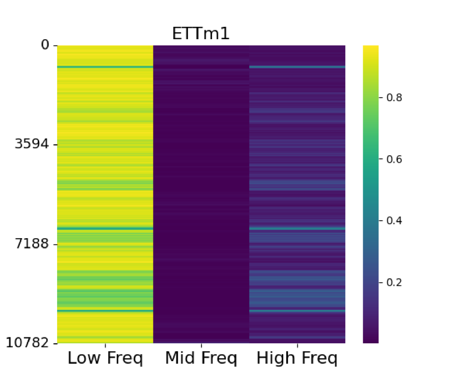
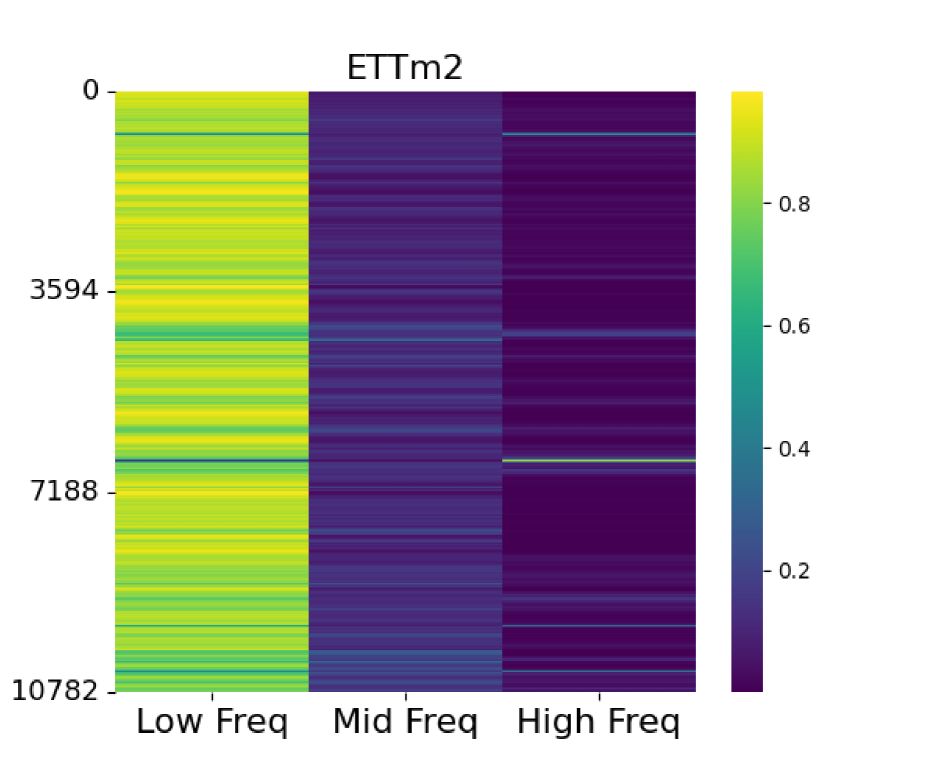
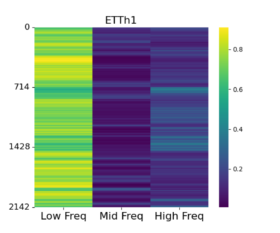
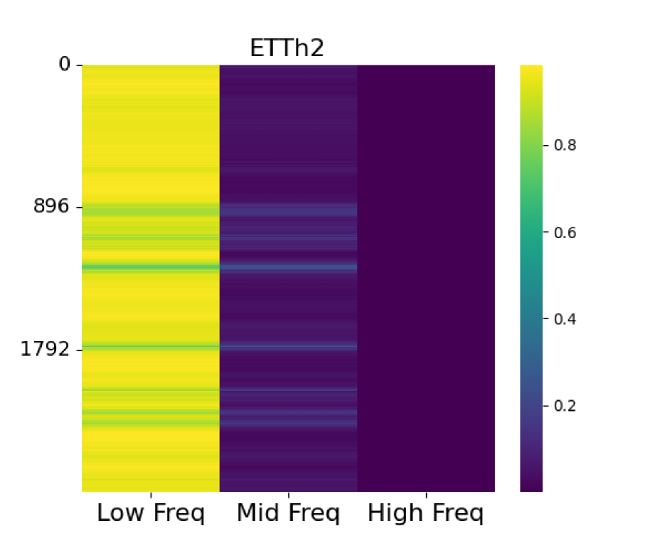
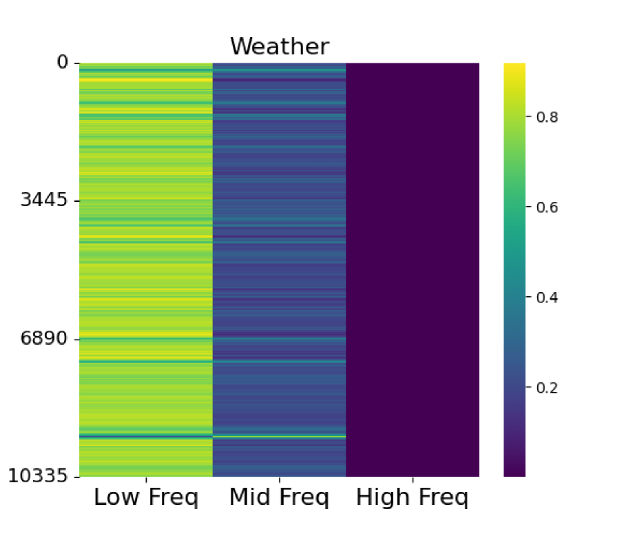
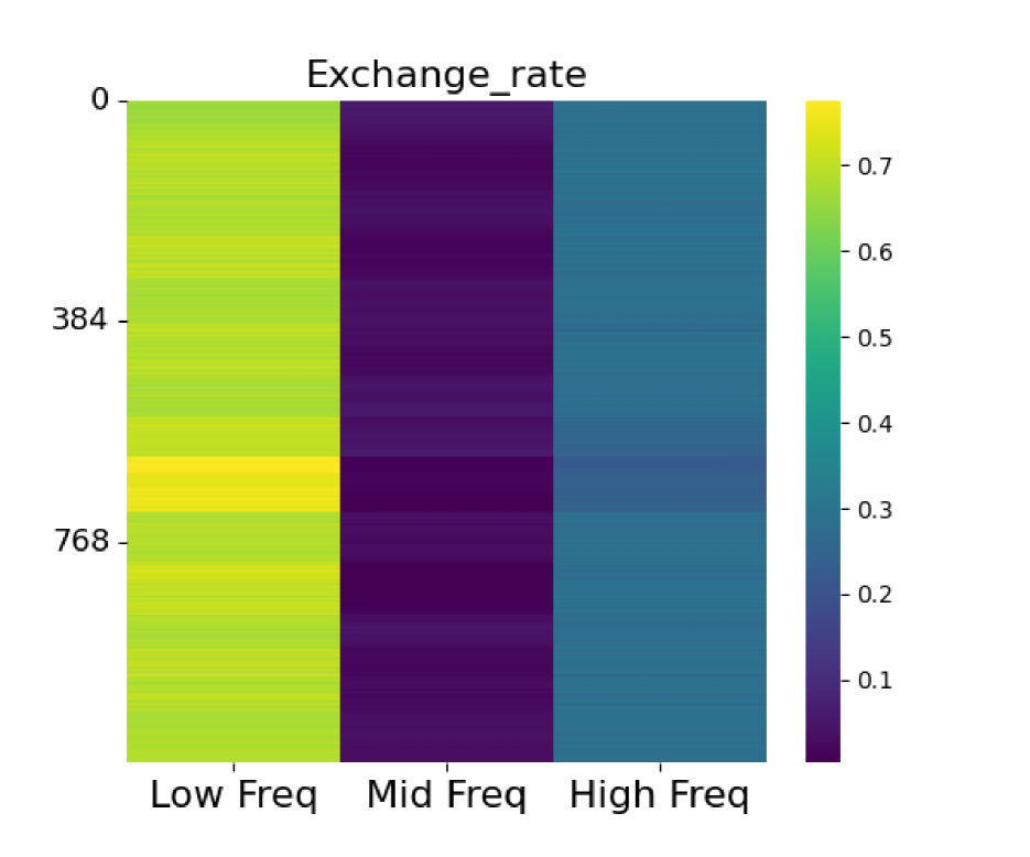
Figure 2: Heatmap representation of gating coefficient sequences across different frequency bands. The X-axis denotes the sequence indices, and the Y-axis represents the frequency bands (experts). The color intensity in each cell corresponds to the gating coefficient, with higher values indicating a greater contribution from the respective frequency band to the prediction of the input sequence.

In addition to the previous ablation study, we conducted an experiment to validate the claim in Section 2.2 that excessive low-pass filtering results in significant information loss. We also systematically examined the impact of different frequency bands on time series forecasting.

In this experiment, we set the prediction length to 720 and the Mixture of Experts module to three experts, each responsible for a specific frequency band: low, mid, and high frequencies. Using six standard datasets (ETTm1, ETTm2, ETTh1, ETTh2, Weather(Angryk et al.,, 2020), and Exchange Rate), we trained the model, extracted the gating coefficients for each expert on the test set, and visualized them in Figure 2 as a heatmap. The X-axis shows frequency bands (experts), the Y-axis represents sequence indices, and the cell values indicate gating coefficients. This visualization highlights how different frequency bands influence each sequence, with higher values indicating greater importance of a specific band.

In the ETTm1 dataset, the heatmap shows the highest gating factor overall in the low frequency band, indicating that the main temporal pattern is concentrated in this band, while the high frequency band plays a role in the final phase of the dataset. Similarly, in the ETTm2 dataset, the low-frequency band has the greatest impact, with most of the signal strength concentrated in this band, while the mid- and high-frequency bands have less of an impact.The ETTh1 dataset exhibits a similar pattern, with both the low-frequency and high-frequency bands making some contribution, while the mid-frequency band has very little impact.The low-frequency band of the ETTh2 dataset is particularly important, which underscores the fact that the low-frequency band has more of an impact on the model predictions. In the weather dataset, both the low and mid-frequency bands have a strong contribution to the predictions. In contrast, for the Exchange_rate dataset, the low and high frequency bands play an important role at different stages, while the low frequency band contains relatively more model information.In summary, the low-frequency band does contains essential information, but Figure 2shows that the mid- and high-frequency bands also hold valuable information that should not be disregarded.

The diverse distribution of coefficients across different frequency bands indicates that the contribution of various components to the prediction is highly context-dependent on the specific data. This underscores the importance of not blindly applying filters prior to experimentation. This finding further validates the argument presented in Section 2.2 and indirectly supports the effectiveness of our proposed Frequency Decomposition MoE module.

5.2.5 Efficiency analysis

In our experiment, we compare our proposed model, FreqMoE, with DLinear, PatchTST and FEDformer on the ETTh1 dataset, fixing the input length at 96, where n represents the number of prediction blocks. Since the backbone of our model is complex-domain MLP, it is significantly more lightweight compared to other Transformer-based models. The number of parameters for each model is detailed in Table 4. Despite having fewer parameters, FreqMoE achieves competitive accuracy in forecasting tasks.

Table 4: Comparison of the number of parameters

Models	Params
FreqMoE (n=1)	14.5K
FreqMoE (n=3)	43.2K
FreqMoE (n=5)	71.9k
Dlinear	18.6K
PatchTST	6.9M
FEDformer	16.8M

6 Conclusion

We introduce the Frequency Decomposition Expert Mixed Model, a new approach for time series forecasting. By decomposing the time series data in the frequency domain and assigning different frequency bands to specialized experts, the frequency band information is fully preserved and utilized. A dynamic gating mechanism adjusts the contribution of each frequency band (expert) according to the frequency characteristics of the input data, and stackable blocks of residuals iteratively refine the predictions. Our empirical results show that the frequency decomposition expert mixture model significantly outperforms existing models on various benchmark datasets.

 

FreqMoE: Enhancing Time Series Forecasting through Frequency Decomposition Mixture of Experts:
Supplementary Materials

 

Appendix A DATASET DESCRIPTION

In this section, we briefly describe the seven real-world datasets used in the experiments, an overview of which is given in Table 5.

Table 5: Overview of datasets.

Dataset	Dim	Timestep	Prediction Length	Frequency
ETTh1	7	17420	{96,192,336,720}	Hour
ETTh2	7	17420	{96,192,336,720}	Hour
ETTm1	7	69680	{96,192,336,720}	15 Minutes
ETTm2	7	69680	{96,192,336,720}	15 Minutes
Weather	21	52696	{96,192,336,720}	10 Minutes
Exchange	8	7588	{96,192,336,720}	Hour
ECL	321	26304	{96,192,336,720}	Hour

The ETT dataset consists of six load sequences and one oil temperature sequence, focusing on relevant time series analysis of the power system. The meteorological dataset covers 21 meteorological variables and records a wealth of meteorological information within the entire year 2020, with a data frequency of every 10 minutes, and all data are collected by the weather stations of the Max Planck Institute for Biogeochemistry. The exchange rate dataset, on the other hand, provides daily exchange rate data for eight countries over the period from 1990 to 2016, revealing trends in national currency exchange rates over time. Finally, the ECL dataset contains electricity consumption data for 321 customers, collected since January 1, 2011, covering a large number of variables and complex temporal patterns.

Appendix B IMPLEMENT DETAIL

B.1 Experiment Detail

In the experiment, we split the ETTh dataset into training, validation, and testing sets in a ratio of 6:2:2, while the other three datasets are divided in a ratio of 7:2:1. The FreqMoE model is implemented using PyTorch(Paszke et al.,, 2019) and conducted the experiments on a computer equipped with an NVIDIA RTX 3090 GPU with 20GB of memory. Each experiment is repeat three times with different random seed, making ensure the consistency of the results. During the model optimization process, the Adam optimizer is employed(Kingma,, 2014), with a default training duration of 40 epochs and a patience setting of 6 for implementing early stopping. Additionally, the learning rate is reduced to half of its previous value after each training iteration.

B.2 Hyperparameters

In our FreqMoE model, there are three key hyperparameters. The number of experts in the frequency decomposition Mixture of Experts module. The number of prediction blocks in the frequency domain prediction module. And the dropout rate for the two complex linear layers within each prediction block. These three important hyperparameters, along with the selection ranges for other hyperparameters, are detailed in Table 6.

Table 6: Hyperparameters used in the FreqMoE model.

Parameter	Value
Expert num	2, 3, 4, 5, 6, 7, 8, 9, 10
Prediction block num	1, 2, 3
Dropout rate	0.2, 0.3, 0.4
Batch size	8, 32, 64, 128
Initial learning rate	0.001, 0.0005, 0.0001
Prediction length	96, 192, 336, 720

In addition, during the experimental process, we observed that selecting a smaller batch size can yield a slight improvement in model performance for the ETTh dataset. Furthermore, regarding the choice of the number of experts, we recommend using 3, 5, 8, or 10 experts, as these configurations typically result in optimal performance.

B.3 Baseline Model

Here is a brief description of the baseline models used in this paper.

1. iTransformer (Liu et al.,, 2024) is a Transformer-based model that embeds variable tokens at individual time points to capture correlations between multiple variables by applying attention mechanisms to inverted dimensions. The source code is available at: https://github.com/thuml/iTransformer.

2. PatchTST (Nie et al.,, 2023) PatchTST is a Transformer-based model that improves long-time prediction accuracy by dividing the time series into subsequence-level patches as input tokens and by using channel-independent techniques. The source code is available at: https://github.com/yuqinie98/PatchTST.

3. Crossformer (Zhang and Yan,, 2023) is a Transformer-based model that efficiently captures inter-temporal and inter-dimensional dependencies by embedding the time series as a two-dimensional vector array, preserving both temporal and dimensional information. The source code is available at: https://github.com/Thinklab-SJTU/Crossformer.

4. TiDE (Das et al.,, 2024) is a MLP-based encoder-decoder model architecture that matches the performance of Transformer-based models on LSTF tasks. The source code is available at: https://github.com/google-research/google-research/tree/master/tide.

5. TimesNet (Wu et al.,, 2023) is a CNN-based model, efficiently capture complex time-varying features by converting a one-dimensional time series into a two-dimensional tensor. The source code is available at: https://github.com/thuml/TimesNet.

6. DLinear (Zeng et al.,, 2022) is a MLP-based model with only one simple linear layer. The source code is available at: https://github.com/cure-lab/LTSF-Linear

7. SCINet (Liu et al.,, 2022) is an CNN-based model that extracted different temporal features from downsampled subsequence by using multiple convolutional filters in each layer. The source code is available at: https://github.com/cure-lab/SCINet

8. FEDformer (Zhou et al., 2022b, ) is a Transformer-based model is a Transformer-based model proposing seasonaltrend decomposition and exploiting the sparsity of time series in the frequency domain. The source code is available at: https://github.com/DAMO-DI-ML/ICML2022-FEDformer.

9. Autoformer (Wu et al.,, 2022) is a Trasnformer-based model address the lack of long-term dependencies by introducing an auto-correlation mechanism and an asymptotic decomposition architecture. The source code is available at: https://github.com/thuml/Autoformer.

Appendix C ADDITIONAL EXPERIMENTS RESULT

C.1 Full Result of Comparison Expertiment

Due to the space limitation of the main text, we place the full results of forecasting in Table 7. The prediction lengths $S\in\{96,192,336,720\}$ and the lookback length is fixed as $T=96$.

Models		FreqMoE		iTransformer		PatchTST		Crossformer		TiDE		TimesNet		DLinear		SCINet		FEDformer		Autoformer
Metric		MSE	MAE	MSE	MAE	MSE	MAE	MSE	MAE	MSE	MAE	MSE	MAE	MSE	MAE	MSE	MAE	MSE	MAE	MSE	MAE
ETTm1	96	0.314	0.356	0.334	0.368	0.329	0.367	0.404	0.426	0.364	0.387	0.338	0.375	0.345	0.372	0.418	0.438	0.379	0.419	0.505	0.475
	192	0.356	0.380	0.377	0.391	0.367	0.385	0.450	0.451	0.398	0.404	0.374	0.387	0.380	0.389	0.439	0.450	0.426	0.441	0.553	0.496
	336	0.385	0.404	0.426	0.420	0.399	0.410	0.532	0.515	0.428	0.425	0.410	0.411	0.413	0.413	0.490	0.485	0.445	0.459	0.621	0.537
	720	0.446	0.445	0.491	0.459	0.454	0.439	0.666	0.589	0.487	0.461	0.478	0.450	0.474	0.453	0.595	0.550	0.543	0.490	0.671	0.561
	Avg	0.375	0.396	0.407	0.410	0.387	0.400	0.513	0.496	0.419	0.419	0.400	0.406	0.403	0.407	0.485	0.481	0.448	0.452	0.588	0.517
ETTm2	96	0.173	0.266	0.180	0.264	0.175	0.259	0.287	0.366	0.207	0.305	0.187	0.267	0.193	0.292	0.286	0.377	0.203	0.287	0.255	0.339
	192	0.235	0.310	0.250	0.309	0.241	0.302	0.414	0.492	0.290	0.364	0.249	0.309	0.284	0.362	0.399	0.445	0.269	0.328	0.281	0.340
	336	0.290	0.350	0.311	0.348	0.305	0.343	0.597	0.542	0.377	0.422	0.321	0.351	0.369	0.427	0.637	0.591	0.325	0.366	0.339	0.372
	720	0.385	0.424	0.412	0.407	0.402	0.400	1.730	1.042	0.558	0.524	0.408	0.403	0.554	0.522	0.960	0.735	0.421	0.415	0.433	0.432
	Avg	0.270	0.337	0.288	0.332	0.281	0.326	0.757	0.610	0.358	0.404	0.291	0.333	0.350	0.401	0.571	0.537	0.305	0.349	0.327	0.371
ETTh1	96	0.371	0.388	0.386	0.405	0.414	0.419	0.423	0.448	0.479	0.464	0.384	0.402	0.386	0.400	0.654	0.599	0.376	0.419	0.449	0.459
	192	0.426	0.422	0.441	0.436	0.460	0.445	0.471	0.474	0.525	0.492	0.436	0.429	0.437	0.432	0.719	0.631	0.420	0.448	0.500	0.482
	336	0.475	0.447	0.487	0.458	0.501	0.466	0.570	0.546	0.565	0.515	0.491	0.469	0.481	0.459	0.778	0.659	0.459	0.465	0.521	0.496
	720	0.488	0.459	0.503	0.491	0.500	0.488	0.653	0.621	0.594	0.558	0.521	0.500	0.519	0.516	0.836	0.699	0.506	0.507	0.514	0.512
	Avg	0.440	0.429	0.454	0.447	0.469	0.454	0.529	0.522	0.541	0.507	0.458	0.450	0.456	0.452	0.747	0.647	0.440	0.460	0.496	0.487
ETTh2	96	0.287	0.337	0.297	0.349	0.302	0.348	0.745	0.584	0.400	0.440	0.340	0.374	0.333	0.387	0.707	0.621	0.358	0.397	0.346	0.388
	192	0.361	0.386	0.380	0.400	0.388	0.400	0.877	0.656	0.528	0.509	0.402	0.414	0.477	0.476	0.860	0.689	0.429	0.439	0.456	0.452
	336	0.407	0.423	0.428	0.432	0.426	0.433	1.043	0.731	0.643	0.571	0.452	0.452	0.594	0.541	1.000	0.744	0.496	0.487	0.482	0.486
	720	0.414	0.438	0.427	0.445	0.431	0.446	1.104	0.763	0.874	0.679	0.462	0.468	0.831	0.657	1.249	0.838	0.463	0.474	0.515	0.511
	Avg	0.367	0.397	0.383	0.407	0.387	0.407	0.942	0.684	0.611	0.550	0.414	0.427	0.559	0.515	0.954	0.723	0.437	0.449	0.450	0.459
Exchange	96	0.080	0.198	0.086	0.206	0.088	0.205	0.256	0.367	0.094	0.218	0.107	0.234	0.088	0.218	0.267	0.396	0.148	0.278	0.197	0.323
	192	0.170	0.293	0.177	0.299	0.176	0.299	0.470	0.509	0.184	0.307	0.226	0.344	0.176	0.315	0.351	0.459	0.271	0.315	0.300	0.369
	336	0.299	0.392	0.331	0.417	0.301	0.397	1.268	0.883	0.349	0.431	0.367	0.448	0.313	0.427	1.324	0.853	0.460	0.427	0.509	0.524
	720	0.826	0.693	0.847	0.691	0.901	0.714	1.767	1.068	0.852	0.698	0.964	0.746	0.839	0.695	1.058	0.87	1.195	0.695	1.447	0.941
	Avg	0.343	0.394	0.360	0.403	0.367	0.404	0.940	0.707	0.370	0.413	0.416	0.443	0.354	0.414	0.750	0.626	0.519	0.429	0.613	0.539
Weather	96	0.168	0.215	0.174	0.214	0.177	0.218	0.158	0.230	0.202	0.261	0.172	0.220	0.196	0.255	0.221	0.306	0.217	0.296	0.266	0.336
	192	0.212	0.253	0.221	0.254	0.225	0.259	0.206	0.277	0.242	0.298	0.219	0.261	0.237	0.296	0.261	0.340	0.276	0.336	0.307	0.367
	336	0.268	0.291	0.278	0.296	0.278	0.297	0.272	0.335	0.287	0.335	0.280	0.306	0.283	0.335	0.309	0.378	0.339	0.380	0.359	0.395
	720	0.342	0.345	0.358	0.349	0.354	0.348	0.398	0.418	0.351	0.386	0.365	0.359	0.345	0.381	0.377	0.427	0.403	0.428	0.419	0.428
	Avg	0.247	0.276	0.258	0.279	0.259	0.281	0.259	0.315	0.271	0.320	0.259	0.287	0.265	0.317	0.292	0.363	0.309	0.360	0.338	0.382
ECL	96	0.152	0.246	0.148	0.240	0.181	0.270	0.219	0.314	0.237	0.329	0.168	0.272	0.197	0.282	0.247	0.345	0.193	0.308	0.201	0.317
	192	0.165	0.255	0.162	0.253	0.188	0.274	0.231	0.322	0.236	0.330	0.184	0.289	0.196	0.285	0.257	0.355	0.201	0.315	0.222	0.334
	336	0.181	0.274	0.178	0.269	0.204	0.293	0.246	0.337	0.249	0.344	0.198	0.300	0.209	0.301	0.269	0.369	0.214	0.329	0.231	0.338
	720	0.219	0.307	0.225	0.317	0.246	0.324	0.280	0.363	0.284	0.373	0.220	0.320	0.245	0.333	0.299	0.390	0.246	0.355	0.254	0.361
	Avg	0.179	0.270	0.178	0.270	0.205	0.290	0.244	0.334	0.251	0.344	0.192	0.295	0.212	0.300	0.268	0.365	0.214	0.327	0.227	0.338
$1^{\text{st}}$ Count		27	24	4	5	0	6	2	0	0	0	0	0	0	0	0	0	2	0	0	0

Table 7: Long-term multivariate forecasting results with prediction lengths $S\in\{96,192,336,720\}$ and fixed lookback length $T=96$. The best forecasting results are in bold and the second-best are underlined. Lower MSE/MAE indicates more accurate predictions.The results of other models are sourced from iTransformer(Liu et al.,, 2024).

As can be seen from Table 7, our model achieves the best results in 51 out of 70 metrics. Among them, FreqMoE performs particularly well on low-channel datasets such as the ETTh (7-channel) and Exchange (8-channel) datasets, demonstrating the good fitness of our frequency domain decomposition prediction model in low-channel scenarios. In contrast, on high-channel datasets such as Weather and ECL, the performance of the model is largely weaker than Transformer-based models such as iTransformer and PatchTST, which may indicate that there is still room for improvement in the extraction of multi-dimensional dependency information by linear models. However, it is worth noting that the model still performs well in multi-dimensional long time prediction, which indicates that the frequency domain decomposition module plays an important role in major frequency band feature extraction.

C.2 Analysis of MoE Ablation Experiment

As the number of experts increases, the performance of the model not only fails to improve, but also declines. We believe that this phenomenon is mainly caused by the following two factors:

1. Frequency range fragmentation: As the number of experts increases, the frequency range that each expert is responsible for becomes narrower, resulting in insufficient information contained within each frequency band to provide adequate feature representation.

2. Uneven allocation of weights in the gating network: There is an imbalance in the allocation of weights in the gating network, with experts responsible for wider frequency ranges and containing more information being given higher weights, while other experts are given relatively lower weights. This unbalanced allocation of weights results in information in some frequency bands not being fully utilized or ignored, leading to loss of information.

In order to verify the effect of the first factor mentioned above, we trained the models with the number of experts 2, 3, 5 and 8, and recorded the band boundaries and the final loss values for each model, by keeping the other hyperparameters of the model constant. In addition, we calculated the width of each frequency band. All the results are shown in Figure 3.

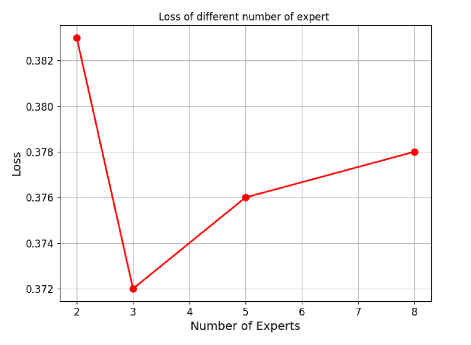
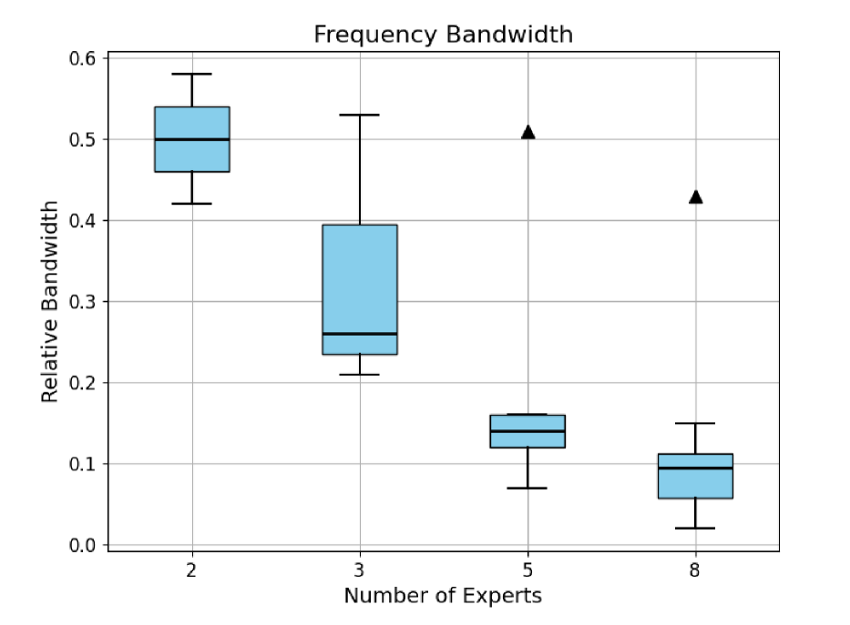
Figure 3: The subplot on the left shows the loss for models with different numbers of experts, and the subplot on the right shows the distribution of the bandwidths of the models with different numbers of experts, where the widths are the relative widths of the bands with respect to the sequence.

It can be clearly seen that as the number of experts increases, the average value of the bandwidth that each expert is responsible for decreases rapidly. When the number of experts increases to 8, except for one expert whose bandwidth is 0.43, the width of the rest of the bands is even less than 0.1. This extremely narrow bandwidth obviously leads to the amount of information contained in it being too small, thus affecting the judgment ability of the gating mechanism and weakening the performance of the model. This result validates the first factor.

To validate the second factor, we again trained a model containing eight experts and up-calculated the mean of the coefficients for each expert and the width of the band for which each expert was responsible on the test set. Figure 4 illustrates the relationship between the mean value of the coefficients for each expert and their corresponding bandwidths.

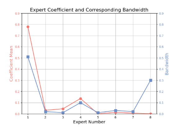
Figure 4: This figure illustrates the average coefficient assigned to each expert by the gating network, along with the bandwidth managed by each expert.

From the results, it can be seen that the experts responsible for wider frequency bands were given higher weights to some extent, while the experts with narrower frequency bands were assigned smaller weights by the gating mechanism due to their low information content. This phenomenon suggests that the gating network tends to assign higher weights to the experts responsible for the more information-rich bands, which leads to result in some of the band information being underutilized. This result validates the second factor we proposed.

C.3 Comparison of Gating Mechanism and Fix Learnable Parameter

To demonstrate the effectiveness of gating mechanism in frequency decomposition module, we conduct the ablation experiment of it, the result are shown in Table 8 as follow.

Table 8: Performance comparison of models using gating mechanism and using fixed learnable parameter.The best results are in bold.

Dataset	Model	Gate Mechanism		Fixed Parameter
	Metric	MSE	MAE	MSE	MAE
ETTH1	96	0.371	0.388	0.375	0.398
	192	0.426	0.422	0.428	0.431
	336	0.475	0.447	0.483	0.465
	720	0.488	0.459	0.540	0.420
ETTH2	96	0.287	0.337	0.294	0.364
	192	0.361	0.386	0.369	0.424
	336	0.407	0.430	0.429	0.466
	720	0.414	0.438	0.447	0.488
ETTM1	96	0.314	0.356	0.314	0.357
	192	0.356	0.380	0.357	0.384
	336	0.385	0.404	0.387	0.405
	720	0.446	0.442	0.455	0.450
ETTM2	96	0.173	0.265	0.176	0.269
	192	0.235	0.310	0.239	0.318
	336	0.290	0.350	0.301	0.369
	720	0.385	0.424	0.406	0.448

According to Table 8, the performance of the model using the gating mechanism is much better than that using the fixed parameters, which shows that the gating mechanism contributes greatly to the enhancement of the model generalization ability as well as the extraction of the key frequency modes.

C.4 Robustness Experiment

In addition, we performed robustness tests on all datasets used in our main text comparison experiments. We used three different random seeds (2020, 2021,2022) to ensure that the model parameters were initialized differently each time. Table 9 shows the mean and standard derivation of the MSE and MAE from multiple experiments, according to the table we can see that the variance of all three experiments is small, indicating that the random initialization has a minimal effect on the model, demonstrating the robustness of our model.

Table 9: Multivariate forecasting results with different random seeds(2020,2021,2022) in FreqMoE with lookback length T = 96.

Models		FreqMoE		iTransformer		PatchTST		DLinear
Metric		MSE	MAE	MSE	MAE	MSE	MAE	MSE	MAE
ETTm1	96	0.314$\pm$0.002	0.356$\pm$0.001	0.334	0.368	0.329	0.367	0.505	0.475
	192	0.356$\pm$0.004	0.380$\pm$0.003	0.377	0.391	0.367	0.385	0.553	0.496
	336	0.385$\pm$0.004	0.404$\pm$0.001	0.426	0.420	0.399	0.410	0.621	0.537
	720	0.446$\pm$0.004	0.445$\pm$0.002	0.491	0.459	0.454	0.439	0.671	0.561
	Avg	0.375$\pm$0.003	0.396$\pm$0.001	0.407	0.410	0.387	0.400	0.588	0.517
ETTm2	96	0.173$\pm 0.001$	0.266$\pm 0.001$	0.180	0.264	0.175	0.259	0.339	0.388
	192	0.235$\pm 0.001$	0.310$\pm 0.001$	0.250	0.309	0.241	0.302	0.340	0.371
	336	0.290$\pm 0.001$	0.350$\pm 0.001$	0.311	0.348	0.305	0.343	0.372	0.371
	720	0.385$\pm 0.002$	0.424$\pm 0.002$	0.412	0.407	0.402	0.400	0.459	0.459
	Avg	0.270$\pm 0.001$	0.337$\pm 0.001$	0.288	0.332	0.281	0.326	0.450	0.371
ETTh1	96	0.371$\pm 0.001$	0.388$\pm 0.001$	0.386	0.405	0.414	0.419	0.449	0.459
	192	0.426$\pm 0.001$	0.422$\pm 0.001$	0.441	0.436	0.460	0.445	0.500	0.482
	336	0.475$\pm 0.002$	0.447$\pm 0.003$	0.487	0.458	0.501	0.466	0.521	0.496
	720	0.488$\pm 0.010$	0.459$\pm 0.008$	0.503	0.491	0.500	0.488	0.514	0.512
	Avg	0.440$\pm 0.003$	0.429$\pm 0.003$	0.454	0.447	0.469	0.454	0.496	0.487
ETTh2	96	0.287$\pm 0.001$	0.337$\pm 0.001$	0.297	0.349	0.302	0.348	0.388	0.459
	192	0.361$\pm 0.001$	0.386$\pm 0.001$	0.380	0.400	0.388	0.400	0.452	0.459
	336	0.407$\pm 0.001$	0.423$\pm 0.003$	0.428	0.432	0.426	0.433	0.482	0.459
	720	0.414$\pm 0.005$	0.438$\pm 0.006$	0.427	0.445	0.431	0.446	0.450	0.459
	Avg	0.367$\pm 0.002$	0.397$\pm 0.003$	0.383	0.407	0.387	0.407	0.450	0.459
Exchange	96	0.080$\pm 0.002$	0.198$\pm 0.001$	0.086	0.206	0.088	0.205	0.323	0.539
	192	0.170$\pm 0.005$	0.293$\pm 0.003$	0.177	0.299	0.176	0.299	0.369	0.539
	336	0.299$\pm 0.005$	0.392$\pm 0.012$	0.331	0.417	0.301	0.397	0.524	0.539
	720	0.826$\pm 0.005$	0.693$\pm 0.007$	0.847	0.691	0.901	0.714	0.941	0.539
	Avg	0.343$\pm 0.004$	0.394$\pm 0.005$	0.360	0.403	0.367	0.404	0.539	0.539
Weather	96	0.168$\pm 0.011$	0.215$\pm 0.006$	0.174	0.214	0.177	0.218	0.336	0.428
	192	0.212$\pm 0.005$	0.253$\pm 0.003$	0.221	0.254	0.225	0.259	0.382	0.428
	336	0.268$\pm 0.003$	0.291$\pm 0.002$	0.278	0.296	0.278	0.297	0.395	0.428
	720	0.342$\pm 0.003$	0.345$\pm 0.005$	0.358	0.349	0.354	0.348	0.428	0.428
	Avg	0.247$\pm 0.005$	0.276$\pm 0.003$	0.258	0.279	0.259	0.281	0.382	0.428
ECL	96	0.152$\pm 0.002$	0.246$\pm 0.001$	0.148	0.240	0.181	0.270	0.317	0.338
	192	0.165$\pm 0.001$	0.255$\pm 0.001$	0.162	0.253	0.188	0.274	0.334	0.338
	336	0.181$\pm 0.001$	0.274$\pm 0.001$	0.178	0.269	0.204	0.293	0.338	0.338
	720	0.219$\pm 0.003$	0.307$\pm 0.002$	0.225	0.317	0.246	0.324	0.361	0.338
	Avg	0.179$\pm 0.001$	0.270 $\pm 0.001$	0.178	0.270	0.205	0.290	0.338	0.338

C.5 Impact of the number of Prediction Blocks

In order to explore the effect of the number of prediction blocks connected via residuals on prediction accuracy, we designed and implemented model comparison experiments with different numbers of prediction blocks. While keeping the number of experts in the frequency domain decomposition module unchanged, we tested the performance of the model with the number of prediction blocks of 1, 2 and 3 on the Weather and Exchange datasets, respectively. The experimental results are shown in Table 10.

Table 10: Performance comparison of models using gating mechanism, fixed learnable parameter, and three prediction blocks. The best results are in bold.

Dataset	Model Metric	1 Prediction Block		2 Prediction Block		3 Prediction Block
	Metric	MSE	MAE	MSE	MAE	MSE	MAE
Exchange	96	0.081	0.198	0.083	0.200	0.080	0.198
	192	0.174	0.296	0.185	0.304	0.170	0.293
	336	0.329	0.410	0.309	0.408	0.301	0.396
	720	0.860	0.706	0.846	0.704	0.828	0.697
Weather	96	0.177	0.227	0.168	0.217	0.169	0.220
	192	0.229	0.263	0.218	0.257	0.214	0.255
	336	0.280	0.308	0.269	0.295	0.267	0.291
	720	0.361	0.359	0.350	0.351	0.345	0.349

According to Table 10, it can be seen that a deeper network structure, increasing the number of prediction blocks, especially over a longer prediction horizon, can significantly improve the performance of the model. This is because through residual connectivity, subsequent prediction blocks are able to focus on frequency modes that were not captured by the previous prediction block, thus making fuller use of information from all frequency bands to iteratively optimize the prediction results.

Appendix D Source Code

The code associated with this paper can be found at: https://anonymous.4open.science/r/FreqMoE-main-077F/README.md

References

- Angryk et al., (2020) Angryk, R. A., Martens, P. C., Aydin, B., Kempton, D., Mahajan, S. S., Basodi, S., Ahmadzadeh, A., Cai, X., Filali Boubrahimi, S., Hamdi, S. M., et al. (2020). Multivariate time series dataset for space weather data analytics. Scientific data, 7(1):227.
- Ariyo et al., (2014) Ariyo, A. A., Adewumi, A. O., and Ayo, C. K. (2014). Stock price prediction using the arima model. In 2014 UKSim-AMSS 16th international conference on computer modelling and simulation, pages 106–112. IEEE.
- Box et al., (2015) Box, G. E., Jenkins, G. M., Reinsel, G. C., and Ljung, G. M. (2015). Time series analysis: forecasting and control. John Wiley & Sons.
- Brigham and Morrow, (1967) Brigham, E. O. and Morrow, R. (1967). The fast fourier transform. IEEE spectrum, 4(12):63–70.
- Das et al., (2024) Das, A., Kong, W., Leach, A., Mathur, S., Sen, R., and Yu, R. (2024). Long-term forecasting with tide: Time-series dense encoder.
- Gardner Jr, (1985) Gardner Jr, E. S. (1985). Exponential smoothing: The state of the art. Journal of forecasting, 4(1):1–28.
- Khan et al., (2020) Khan, Z. A., Hussain, T., Ullah, A., Rho, S., Lee, M., and Baik, S. W. (2020). Towards efficient electricity forecasting in residential and commercial buildings: A novel hybrid cnn with a lstm-ae based framework. Sensors, 20(5):1399.
- Kingma, (2014) Kingma, D. P. (2014). Adam: A method for stochastic optimization. arXiv preprint arXiv:1412.6980.
- Li and Zong, (2012) Li, J. F. and Zong, Q. (2012). The forecasting of the elevator traffic flow time series based on arima and gp. In Advances in Mechanics Engineering, volume 588 of Advanced Materials Research, pages 1466–1471. Trans Tech Publications Ltd.
- Liu et al., (2022) Liu, M., Zeng, A., Chen, M., Xu, Z., Lai, Q., Ma, L., and Xu, Q. (2022). Scinet: Time series modeling and forecasting with sample convolution and interaction.
- Liu et al., (2024) Liu, Y., Hu, T., Zhang, H., Wu, H., Wang, S., Ma, L., and Long, M. (2024). itransformer: Inverted transformers are effective for time series forecasting.
- Liu et al., (2023) Liu, Y., Li, C., Wang, J., and Long, M. (2023). Koopa: Learning non-stationary time series dynamics with koopman predictors.
- Nelson, (1998) Nelson, B. K. (1998). Time series analysis using autoregressive integrated moving average (arima) models. Academic emergency medicine, 5(7):739–744.
- Nie et al., (2023) Nie, Y., Nguyen, N. H., Sinthong, P., and Kalagnanam, J. (2023). A time series is worth 64 words: Long-term forecasting with transformers.
- Oreshkin et al., (2020) Oreshkin, B. N., Carpov, D., Chapados, N., and Bengio, Y. (2020). N-beats: Neural basis expansion analysis for interpretable time series forecasting.
- Paszke et al., (2019) Paszke, A., Gross, S., Massa, F., Lerer, A., Bradbury, J., Chanan, G., Killeen, T., Lin, Z., Gimelshein, N., Antiga, L., et al. (2019). Pytorch: An imperative style, high-performance deep learning library. Advances in neural information processing systems, 32.
- Vaswani, (2017) Vaswani, A. (2017). Attention is all you need. Advances in Neural Information Processing Systems.
- Wang et al., (2024) Wang, S., Wu, H., Shi, X., Hu, T., Luo, H., Ma, L., Zhang, J. Y., and Zhou, J. (2024). Timemixer: Decomposable multiscale mixing for time series forecasting.
- Wu et al., (2023) Wu, H., Hu, T., Liu, Y., Zhou, H., Wang, J., and Long, M. (2023). Timesnet: Temporal 2d-variation modeling for general time series analysis.
- Wu et al., (2022) Wu, H., Xu, J., Wang, J., and Long, M. (2022). Autoformer: Decomposition transformers with auto-correlation for long-term series forecasting.
- Xu et al., (2024) Xu, Z., Zeng, A., and Xu, Q. (2024). Fits: Modeling time series with parameters.
- Zeng et al., (2022) Zeng, A., Chen, M., Zhang, L., and Xu, Q. (2022). Are transformers effective for time series forecasting?
- Zeroual et al., (2020) Zeroual, A., Harrou, F., Dairi, A., and Sun, Y. (2020). Deep learning methods for forecasting covid-19 time-series data: A comparative study. Chaos, solitons & fractals, 140:110121.
- Zhang et al., (2024) Zhang, X., Zhao, S., Song, Z., Guo, H., Zhang, J., Zheng, C., and Qiang, W. (2024). Not all frequencies are created equal:towards a dynamic fusion of frequencies in time-series forecasting.
- Zhang and Yan, (2023) Zhang, Y. and Yan, J. (2023). Crossformer: Transformer utilizing cross-dimension dependency for multivariate time series forecasting. In The eleventh international conference on learning representations.
- Zhou et al., (2021) Zhou, H., Zhang, S., Peng, J., Zhang, S., Li, J., Xiong, H., and Zhang, W. (2021). Informer: Beyond efficient transformer for long sequence time-series forecasting.
- (27) Zhou, T., Ma, Z., Wen, Q., Sun, L., Yao, T., Yin, W., Jin, R., et al. (2022a). Film: Frequency improved legendre memory model for long-term time series forecasting. Advances in neural information processing systems, 35:12677–12690.
- (28) Zhou, T., Ma, Z., Wen, Q., Wang, X., Sun, L., and Jin, R. (2022b). Fedformer: Frequency enhanced decomposed transformer for long-term series forecasting.
- Zhu et al., (2023) Zhu, X., Xiong, Y., Wu, M., Nie, G., Zhang, B., and Yang, Z. (2023). Weather2k: A multivariate spatio-temporal benchmark dataset for meteorological forecasting based on real-time observation data from ground weather stations.
- Zufferey et al., (2017) Zufferey, T., Ulbig, A., Koch, S., and Hug, G. (2017). Forecasting of smart meter time series based on neural networks. In Data Analytics for Renewable Energy Integration: 4th ECML PKDD Workshop, DARE 2016, Riva del Garda, Italy, September 23, 2016, Revised Selected Papers 4, pages 10–21. Springer.