Snapshot Compressed Imaging Based Single-Measurement Computer Vision for Videos

Abstract

Snapshot compressive imaging (SCI) is a promising technique for capturing high-speed video at low bandwidth and low power, typically by compressing multiple frames into a single measurement. However, similar to traditional CMOS image sensor based imaging systems, SCI also faces challenges in low-lighting photon-limited and low-signal-to-noise-ratio image conditions. In this paper, we propose a novel Compressive Denoising Autoencoder (CompDAE) using the STFormer architecture as the backbone, to explicitly model noise characteristics and provide computer vision functionalities such as edge detection and depth estimation directly from compressed sensing measurements, while accounting for realistic low-photon conditions. We evaluate the effectiveness of CompDAE across various datasets and demonstrated significant improvements in task performance compared to conventional RGB-based methods. In the case of ultra-low-lighting (APC $\leq$ 20) while conventional methods failed, the proposed algorithm can still maintain competitive performance.

1 Introduction

Traditional video and image processing and computer vision tasks such as video classification [1], object detection and tracking [2, 3], and depth estimation [4] are accomplished in the RGB space using spatial and temporal samples acquired by image sensors such as active pixel sensors. Such a pipeline involves high pixel sample throughput, processing by Image Signal Processing for de-noising [5, 6], de-mosaicing and other enhancements [7], and introduces high power consumption and latency.

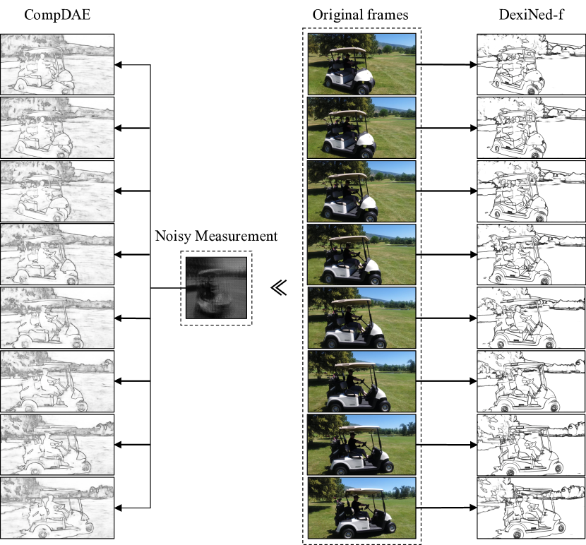
Figure 1: Comparison of our methodology and traditional frame-based methods. (left) Our proposed CompDAE deals with video task directly through low-SNR compressive measurements. (right) Previous method operates on RGB image per frame, demanding higher data bandwidth.

In this paper, we propose a new paradigm for computer vision by training an auto-encoder using raw sensor information acquired using compressive sensing (CS) [8], thereby significantly reduce data bandwidth, power and latency.

We also studied the performance of the proposed system under ultra-low-lighting conditions, when various forms of sensor noise and weak signal strength lead to very low signal-to-noise ratios (SNR). Noise in these scenarios is typically modeled by a Poisson-Gaussian model [9], where the Poisson noise across different frames follows a Poisson process. Photon counts at the same pixel over different time intervals are correlated, and Poisson noise at different times is not entirely independent. As a result, signal aggregation at corresponding pixel positions offers limited noise cancellation. While denoising neural networks [10] are often developed for image denoising, they primarily enhance low-quality images without addressing temporal dependency in Poisson noise.

On the other hand, computer vision based on compressive imaging can be broadly classified into two categories:

The first category of systems perform computer vision related processing after first reconstructing video frames, which involves compressive sensing reconstruction that is usually time-consuming and may lead to information loss [11], both limiting their applicability in real-world applications.

The second category is reconstruction-free, including works such as [12, 13, 14], for infrared imaging [11], autonomous vehicles [15], and action classification [16]. A common limitation of these methods is that they can only perform visual tasks at the rate of compressed snapshot sequences, restricting them to image-level processing rather than multi-frame video processing. While executing video tasks directly in the compressive measurement domain would be ideal, a significant bottleneck in this approach lies in the representation of compressive measurements. In practice, the performance of these tasks in the compressive measurement domain has not met theoretical expectations. Zhang et al. [14] attempted to address this limitation by employing video-domain semantic computer vision (SCV) specifically for regions of interest (ROI), trading off between reconstructing the entire video and the limited performance of the compressive measurement domain. In general, fundamentally improving performance will likely require optimized measurement feature decoders or more advanced neural network architectures with stronger representational capabilities.

To address such challenges, this paper makes the following key contributions:

1. We introduce a Poisson-Gaussian noise measurement model tailored for compressive imaging under photon-limited conditions, effectively addressing the noise complexities encountered in low-light scenarios.

2. We develop a novel Compressive Denoising Autoencoder (CompDAE) framework that learns robust representations directly from compressed measurements, enabling the use of noisy raw measurements for video-level downstream tasks.

3. We demonstrate the effectiveness of our approach through pre-training on a simulated low-SNR dataset with limited frames, achieving notable generalization in edge detection and monocular depth estimation.

2 Related work

Snapshot Compressive Imaging

is an advanced imaging technique that captures a sequence of video frames in a single shot using a two-dimensional detector, incorporating compressive sensing principles. In the reconstruction stage, the video SCI reconstruction solves an ill-posed inverse problem. Traditional model-based reconstruction algorithms combines the idea of iterative optimization but requiring a variety of prior knowledge, such as total variation (TV) [17], non-local low rank [18] and so on. In recent years, learning-based models, particularly Transformers [19] have been introduced to SCI reconstruction by exploring long-term dependencies [20, 21].

Optimal sensing matrices or binary masks have also been studied using learning-based approaches. The DeepBinaryMask model [22] proposes an end-to-end neural network framework for video compressive sensing, where the sensing matrix (coded mask) is optimized as weights alongside the reconstruction process.

Denoising Autoencoders (DAEs) are a class of autoencoders that corrupt a signal for learning representations by reconstructing the original, uncorrupted signal [23]. For example, a naive DAE consists of an encoder $f(\cdot)$ and a decoder $g(\cdot)$, which work together to minimize a loss function $\mathcal{L}(x,g(f(x_{noisy})))$. By mapping the input $x_{noisy}$ to a latent representation $z=f(x_{noisy})$ and then decoding $z$ to reconstruct the clean input $x$, the autoencoder learns the underlying structure of the data $x_{noisy}$, allowing it to extract informative feature representations.

Denoising and masked autoencoding methods for computer vision have seen continuous progress [24, 25, 26, 27]. Recent approaches leverage Transformer architectures [28] to unify vision and language tasks. iGPT [25] used pixels as tokens, while ViT [26] used patches as tokens, establishing robust Transformer models for vision and exploring masked prediction with patches. MAE [27] returns to the core of DAEs, emphasizing the importance of decoding.

Our CompDAE is a form of denoising autoencoding, but different from the classical DAE in a number of ways. The objective of CompDAE is to minimize $\mathcal{L}(x,g(f(y_{noisy})))$ which not only reconstructs the original video sequence but also removes noise from the input compressive measurements $y_{noisy}$.

Self-supervised Learning has emerged as a transformative paradigm in computer vision, allowing models to learn from vast amounts of unlabeled data. This paradigm enables the development of robust visual representations without the need for extensive human-labeled datasets, which are often costly and time-consuming to create. This is achieved by defining pretext tasks that leverage the inherent structure of the data. For instance, a model might learn to predict the missing parts of an image [24, 25, 27] or to reconstruct an image from its colorized version [29]. By solving these tasks, the model learns valuable representations that can be applied to various downstream tasks such as image classification [27].

3 Single Measurement SCI-based Computer Vision in Low-Lighting Conditions

Our goal is to transfer knowledge from snapshot compressive imaging (SCI) to downstream video tasks, particularly in ultra-low-lighting photon-limited scenarios. In image processing, DAEs are especially effective at learning latent representations that remove noise from noisy inputs while preserving important structural details. In this section, we first introduce our low-light noisy measurement generation pipeline, followed by the architecture of the proposed Compressive Denoising Autoencoder (CompDAE) model.

3.1 Low-light Compressive Imaging Noise

For gray-scale video SCI, we use coded aperture compressive temporal imaging (CACTI) [30] as an example. The high-speed frames of a video sequence are modulated at a higher speed than the capture rate of the camera and then compressed to a single compressed measurement. The dynamic scene is spatially coded by a temporal variant mask, such as different patterns on the digital micro-mirror device (DMD). The number of coded frames for a single measurement is determined by the number of variant codes of the mask or different patterns on the DMD within the integration (exposure) time.

Specifically, consider that $T$ video frames are modulated by $T$ different modulation patterns. Let $\{\mathbf{X}_{t}\}^{T}_{t=1}\in\mathbb{R}^{n_{x}\times n_{y}}$ denote a $T$-frame high-speed scene to be captured in a single exposure time, where $n_{x}$, $n_{y}$ represent the spatial resolution of each frame and $T$ is the compression ratio (Cr) of the video SCI system. Then, the modulation process can be modeled as multiplying $\{\mathbf{X}_{t}\}^{T}_{t=1}$ by pre-defined masks $\{\mathbf{M}_{t}\}^{T}_{t=1}\in\mathbb{R}^{n_{x}\times n_{y}}$,

$$\mathbf{Y}_{t}=\mathbf{X}_{t}\odot\mathbf{M}_{t},$$ (1)

where $\{\mathbf{Y}_{t}\}^{T}_{t=1}\in\mathbb{R}^{n_{x}\times n_{y}}$ and $\odot$ denote the modulated frames and Hadamard (element-wise) product, respectively. Modulated frames are then summed (integrating the light in the imaging system) to a single measurement ${\mathbf{Y}}\in\mathbb{R}^{n_{x}\times n_{y}}$. Thus, the forward model of video SCI system can be formulated as,

$$\mathbf{Y}=\sum^{T}_{t=1}{\mathbf{X}_{t}\odot\mathbf{M}_{t}}+\mathbf{N},$$ (2)

where $\mathbf{N}\in\mathbb{R}^{n_{x}\times n_{y}}$ denotes the measurement noise. In the context of photon-limited applications (such as low-light imaging), the Poisson-Gaussian model is generally used for raw-data digital imaging sensor data  [9]. In general, the noise term is composed of two mutually independent parts, a Poisson signal dependent component $\eta_{p}$ and a Gaussian signal-independent component $\eta_{g}$.

$$\mathbf{Y_{noisy}}=\sum^{T}_{t=1}{\left(\mathbf{X}_{t}\odot\mathbf{M}_{t}+\eta_{p,t}\right)}+\eta_{g}.$$ (3)

The distributions of these two components are characterized as follows, $\alpha(\mathbf{X}_{t}\odot\mathbf{M}_{t}+\eta_{p,t})\sim\mathcal{P}(\alpha(\mathbf{X}_{t}\odot\mathbf{M}_{t}))$, $\eta_{g}\sim\mathcal{N}(0,\sigma)$, where $\alpha>0$ and $\sigma>0$ are real scalar parameters and $\mathcal{P}$ and $\mathcal{N}$ Denote the Poisson and normal distributions.

3.2 From imaging towards vision

Our compressive denoising autoencoder (CompDAE) is a simple DAE approach that reconstructs the original clean spacetime data from its raw temporal compressive measurement captured by SCI sensors. Like all DAE [23], our approach has an encoder that maps the noisy (raw) measurement to a latent representation, and a decoder that reconstructs the original spacetime signal from the latent representation. Inspired by Masked Autoencoder (MAE) [27], we adopt an asymmetric design that allows the encoder to operate on the measurement and modulation masks of SCI system and a lightweight decoder ($N$<$M$/2) that reconstructs the full signal from the latent representation.

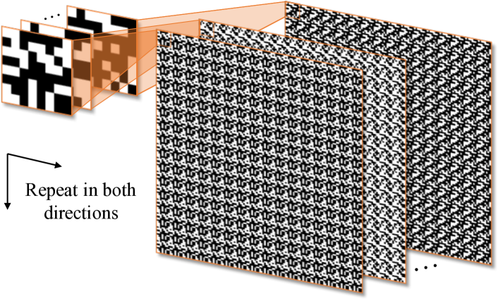
Figure 2: Construction of binary mask pattern.

Random binary patterns Considering real physical constraints, the masks or DMD response of light is always nonnegative and bounded [30, 31]. Moreover, during the implementation of the modulation, practical SCI systems often employ binary-valued masks. Theoretical analysis of binary masks confirms that i.i.d. binary (Bernoulli) masks is feasible for recovery [32]. The probability of non-zero entries $\rho$ is related with the achieved distortion which is a hyperparameter of mask design. As shown in Figure 2, the binary masks used in our CompDAE are generated by spatially replicating a smaller binary sub-mask in both directions.

CompDAE encoder. Following STFormer [20], we use the estimation module to pre-process measurement and masks in the pre-processing stage, inspired by [33, 34]. Just as in a STFormer, our encoder is composed of a token generation block, and a series of STFormer blocks. TG block uses 3D convolution for feature mapping, and then treats each point of the feature map as a token. STFormer blocks explore the spatial and temporal correlation between each token via spatial-temporal self-attention mechanism.

CompDAE decoder. The CompDAE decoder functions as a reconstruction module exclusively during the pre-training phase [33]. The final convolutional layers enable efficient and structured upsampling, generating high-resolution outputs in a smooth and coherent manner. These layers also allow the model to learn localized filters tailored to different image characteristics, such as edge enhancement and noise suppression. This adaptability equips the model to make the precise adjustments required for accurate pixel-level reconstruction.

To address the complexity of transfer learning in downstream tasks, the decoder stacks a series of STFormer blocks before the convolutional block. We apply a partial fine-tuning strategy [27] by fine-tuning only the decoder while keeping the encoder fixed to generate spatiotemporal representation of the compressive measurement. This strategy allows independent design of the decoder architecture. Our experiments utilize small decoders that are shallower than the encoder. With this asymmetrical design, the encoded tokens are only processed by the lightweight decoder, which significantly reduces fine-tuning time.

Reconstruction target Our CompDAE operates directly in the raw measurement domain, requiring the model to effectively extract meaningful representations from noisy measurements. As the average photon count (APC) decreases, the signal-to-noise ratio (SNR) correspondingly declines, resulting in increased noise within the raw measurements. To systematically generate different APC levels for each compressed frame, we normalize the pixel values by calculating the mean of all grayscale pixels and then use these normalized values as the target for pre-training reconstruction. The grayscale frames are then rescaled to a specified APC, and Poisson-Gaussian noise is applied according to Eq.(3). This process enables the generation of low-light measurements with controlled SNR conditions. During pre-training, CompDAE is trained with noisy input measurements, encoding both the measurements and the repeated masks to produce tokenized representations of the video clip. Our loss function computes the mean squared error (MSE) between the reconstructed and original frames in the pixel space. The decoder is initially responsible for pixel reconstruction during pre-training, while in the fine-tuning phase, its role shifts to performing pixel-level classification or regression for specific downstream tasks. The decoder can be formalized as a regression mapping function $g(:)$; in other words, $\hat{X}_{target}=g(z)$, where the latent spatiotemporal tokens are $z$ and $\hat{X}_{target}$ corresponds to the result of the last convolutional layer. In the case of edge detection, $\hat{X}_{target}$ are probability maps of a series of frames, we directly apply the binary cross-entropy loss with logits. For another task, we still compute the MSE loss only on pixels whose depth values are available.

4 Experiment Results

To test the effectiveness of the proposed approach, we conducted self-supervised pre-training using DAVIS2017 [35], the original Train&Val datasets containing 90 videos, for a total of 6242 frames at 480 × 894 spatial resolution. Then we performed supervised training to evaluate the representations with transfer learning for two commonly-used computer vision tasks: (i) edge detection and (ii) monocular depth estimation. As few publicly available datasets support video edge detection, we generated high precision ground truth (GT) edge maps using state-of-the-art model DexiNed [36], whose outputs are fused from multiple intermediate edge maps. To verify model edge-detection performance raw sensor measurement, we tested the fine-tuned model using six benchmark gray-scale datasets (Kobe, Traffic, Runner, Drop, Crash and Aerial with spatial resolution of 256 × 256). The same process was applied over the entire DAVIS2017 and benchmark gray-scale datasets. We employed depth completion to enhance the performance of our model for depth estimation tasks using the KITTI dataset [37]. This approach involves utilizing RGB images to fill in missing depth values in the depth maps, particularly where the depth information is sparse or absent. Then we fine-tuned and testes our model on generated raw measurement from road and lane scenes in KITTI dataset to predict frame-wise depth estimation.

4.1 Implementation Details

We used PyTorch framework with a single NVIDIA A100 GPU (80GB) for training. Following the CACTI imaging process in Sec 3.1, a series of photon-limited measurements were generated. Unless otherwise specified, the default CompDAE had 4 STFormer blocks, only the last 3D convolutional layers could be tuned (decoder depth $N$ = 0), the reconstruction target was original pixels, the data augmentation was random resized cropping and random flipping, low-light factor APC = 20. For all training settings, the Gaussian noise standard deviation $\sigma$ was 0.01. During testing, however, the noise level was adapted to each APC setting, with $\sigma$ set to APC/100, simulating varying noise intensities corresponding to photon-limited conditions. And the pre-training length is 30 epochs in noisy measurement domain (plus 120 epochs in clean measurement domain.) Our default compression setting was 8 frames each with 128 × 128 pixels (i.e., Cr = 8). The 8 frames were sampled from the original video with a temporal stride of 1 or 2 to preserve redundancy within the selected clip, as the underlying assumption of compressive sensing is the compressibility of high-speed video frames due to the similarity between adjacent frames. In the spatial domain, we performed random resized cropping with a scale range of [0.8, 1.2], and random flipping. We used the noisy measurement and masks as inputs to train the CompDAE and use Adam [38] optimizer to optimize the model. And the default initial learning rate was set to 0.0001. To speed up training, we trained the CompDAE on data with a spatial resolution of 128 × 128 (60 epochs) on pre-training and edge detection task fine-tuning. In the depth estimation task, we resized KITTI data with a spatial resolution of 256 × 256 (100 epochs with AdamW [39] optimizer with a batch size of 4) for fine-tuning.

Architecture. Our encoder and decoder are based on standard STFormer architecture [20]. The so called TG block consists of five 3D convolutional layers within spatial downsampling. Thus, for a original 8 × 128 × 128 video clip, this block generates 8 × 64 × 64 tokens. These tokens are then passed through $M$ STFormer blocks of encoder, producing an output that maintains the same dimensions. The decoder part mainly focus on regression in the pixel space. We also study a variant whose decoder contains $N$ STFormer blocks before the reconstruction block. Number $N$ denotes the decoder depth, depending on downstream task difficulty.

Metrics. The performance of CompDAE was evaluated using different metrics, depending on the specific task: (i) Edge Detection: We used the Optimal Dataset Scale (ODS) and Optimal Image Scale (OIS) F1-scores to evaluate the quality of edge detection outputs. (ii) Depth Estimation: We evaluated depth estimation performance using metrics such as Absolute Relative Error (AbsRel), Root Mean Square Error (RMSE), Logarithmic Error ($\log$10), and precisions ($\delta_{1}$, $\delta_{2}$, and $\delta_{3}$). These metrics measured the accuracy of predicted depth-maps compared to the ground truth.

4.2 Comparison with conventional algorithms

We demonstrate the limitations of conventional algorithms for edge detection under ultra-low-light conditions.

As shown in Figure 3, pretrained SOTA DexiNed [36] fails to produce clear edges at decreasing APC, where edge structures become almost indistinguishable due to noise. In contrast, our fine-tuned CompDAE consistently retains clear edge information even at very low APC values, demonstrating strong robustness to noise.

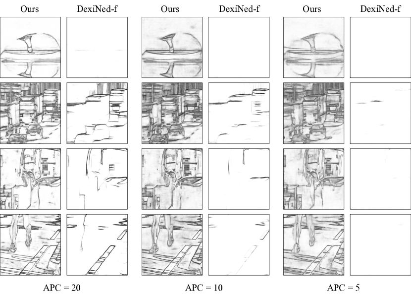
Figure 3: Comparison of edge detection results under different ultra-low-lighting conditions.

We compare our method with previous techniques for edge detection (RCF [40], BDCN [41], DexiNed) and depth estimation (MiDaS v3.1 [4]). Unlike conventional algorithms that operate on clean RGB frames, our approach processes a single compressive measurement under low-SNR conditions, marking a fundamental departure from traditional RGB-based methods. Despite the inherent disadvantage of such comparison, since our input was corrupted by severe low-light limitations while conventional methods rely on clean images, CompDAE consistently outperforms these methods in frame-level performance.

Method	ODS	OIS	Params (M)
Canny	0.473	0.501	-
RCF	0.534	0.569	14.80
BDCN	0.569	0.618	16.30
Ours	0.672	0.685	23.82

Table 1: Evaluation on benchmark grayscale video simulation datasets [42] with our fine-tuned CompDAE.

Method	AbsRel	RMSE	$\log$10	$\delta_{1}$	$\delta_{2}$	$\delta_{3}$
MiDaS [4]	0.638	28.569	1.061	0.499	0.560	0.632
Ours ($N$ = 0)	0.208	5.777	0.283	0.745	0.876	0.941
Ours ($N$ = 1)	0.178	5.823	0.302	0.666	0.867	0.948

Table 2: Fine-tuning and evaluating on KITTI [37] with our pre-trained CompDAE.

As shown in Table 1 and Table 2, we quantitatively compare the performance of CompDAE under an APC = 20 low-light condition against conventional algorithms that use original clean images. In Table 1, CompDAE achieves superior ODS and OIS scores, outperforming edge detection baselines like Canny, RCF, and BDCN despite the challenging low-light input. Similarly, in Table 2, CompDAE demonstrates competitive depth estimation performance on the benchmark KITTI dataset, showing substantial improvement over MiDaS. CompDAE effectively maintains high performance under low-light conditions, bridging the gap with traditional algorithms trained on clean images.

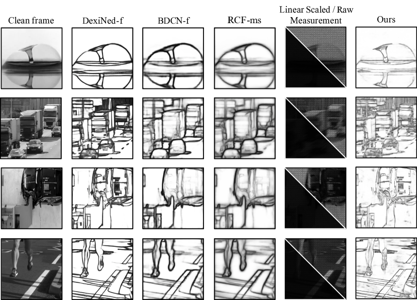
Figure 4: Comparison of edge detection results on several benchmark grayscale video simulation datasets (CompDAE ($N$ = 0) with APC = 20 low-lighting condition; DexiNed, BDCN and RCF with original grayscale frames).

CompDAE was capable of generating multi-frame results for various video tasks in an end-to-end manner. Due to space constraints, we presented visual comparisons only for selected frames from benchmark datasets. In Figure 4, our edge detection results are compared with the DexiNed model and the Canny operator. Remarkably, our results exhibit competitive edge detection accuracy under low-SNR conditions and, notably, produce thinner edges compared to DexiNed.

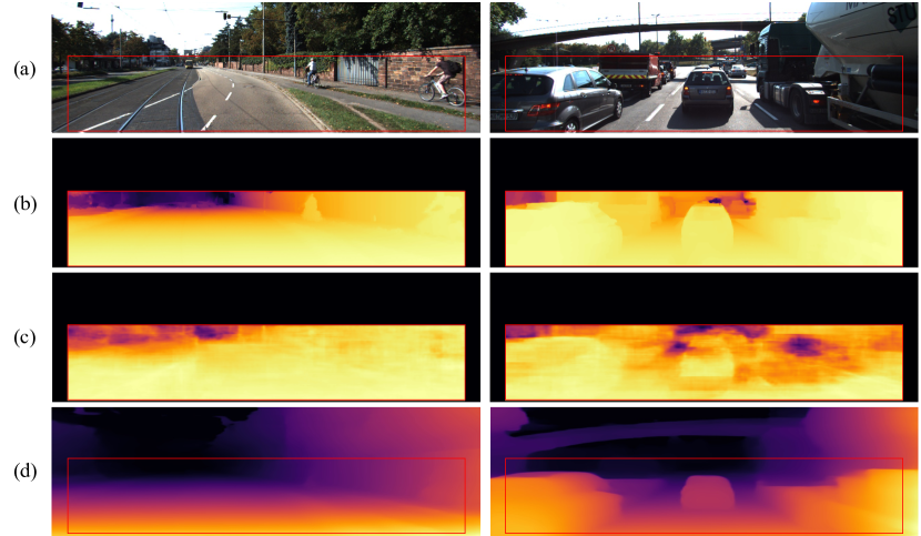
Figure 5: Comparison of depth estimation results. (a) RGB images of original scenes. (b) Groud truth. (c) CompDAE ($N$ = 1) with APC = 20 low-lighting condition. (d) MiDaS with clean RGB.

For the monocular depth estimation task, we randomly selected prediction results from two urban street scenes in KITTI dataset, as shown in Figure 5. The red boxed area indicates the region covered by Lidar scans in the dataset. Our CompDAE displays depth estimation results within this region. Despite the challenges posed by noisy input data, CompDAE is able to provide a reasonably accurate depth estimation. Compared to algorithms operating in the RGB domain, our method does exhibit certain limitations, such as lower resolution, highlighting the challenges of representing stereo information in grayscale compressive measurements.

4.3 Main Properties

We ablate our CompDAE using default settings in Sec 4.1. Several intriguing properties are observed.

Depth	ODS	OIS
0	0.672	0.685
1	0.681	0.694
2	0.695	0.709
3	0.686	0.698

Table 3: Impact of Decoder Depth. Depth refers to the number of fine-tuned STFormer blocks used in the decoder module.

Decoder design As mentioned in Figure LABEL:fig:framework, Decoder depth $N$ represents the number of STFormer blocks used in the reconstruction decoder. To optimize the model, we employ a partial fine-tuning protocol in which the last several blocks are fine-tuned while the others remain frozen [29, 27]. Given our asymmetric design (i.e.,$N$<$M$/2 with $M$ = 4), the decoder remains efficient and flexible. Table 3 shows that increasing depth from 0 to 1 improves ODS and OIS scores, striking a balance between performance and computational efficiency within the asymmetric framework. To examine the effect of further depth, we also tested deeper configurations. A depth of 2 achieves the highest scores (ODS = 0.695, OIS = 0.709), but a depth of 3 shows a slight decline, indicating that additional blocks may add computational cost without practical benefit. Overall, while deeper decoders (e.g., $N$ = 2) can yield marginal gains, the asymmetric configurations ($N$ = 0 or $N$ = 1) offer an effective trade-off between efficiency and quality, making it the optimal choice for applications.

APC	5		10		20
	ODS	OIS	ODS	OIS	ODS	OIS
5	0.644	0.652	0.663	0.670	0.647	0.653
10	-	-	0.650	0.659	0.653	0.663
20	-	-	-	-	0.672	0.685

Table 4: Impact of Average Photon Counts (APC) under Different Noise Conditions.

Measurement Noise Table 4 explores the impact of different APC training settings on CompDAE, where APC represents the average photon counts per frame in photon-limited conditions. Higher APC values simulate scenarios with more photons, implying better lighting and reduced shot noise. Notably, CompDAE demonstrates robust performance across varying testing conditions without requiring model adjustments for changes in noise or photon counts. Models trained with higher APC (e.g., APC = 20) exhibit consistently better adaptability. This stability suggests that CompDAE inherently learns robust features that generalize well, regardless of specific photon or noise levels during testing.

Cr	4		8		16
	ODS	OIS	ODS	OIS	ODS	OIS
4	0.669	0.682	0.587	0.593	0.459	0.497
8	-	-	0.672	0.685	0.513	0.538
16	-	-	-	-	0.612	0.617

Table 5: Impact of Compression Ratio (Cr).

Compression ratio. Table 5 demonstrates the effect of compression ratio (Cr). Here, Cr corresponds to the number of masks utilized in the compressive imaging process, with lower values indicating less compression (higher spatial-temporal fidelity) and higher values indicating greater compression. Our results reveal that a Cr of 8 achieves the best overall performance when used consistently in both training and testing. This moderate compression ratio strikes an optimal balance, capturing sufficient scene dynamics without excessive information loss, thereby enhancing reconstruction accuracy. In contrast, Cr = 16, which involves a higher level of compression, shows the lowest scores, indicating that high compression sacrifices accuracy due to reduced spatial-temporal information. Additionally, training and testing with consistent Cr values, particularly at Cr = 4 or Cr = 8, enhances model performance, while mismatched compression ratios across training and testing lead to notable performance drops. These findings underscore the importance of aligning Cr settings during both phases for effective generalization.

$\rho$	ODS	OIS
0.3	0.673	0.680
0.4	0.638	0.652
0.5	0.672	0.685

Table 6: Impact of Mask Pattern Density $\rho$.

Non-zero density. Table 6 presents the model performance with varying mask pattern densities, denoted by $\rho$, which is the probability of non-zero entities in the binary mask pattern. Higher values of $\rho$ allow more light to pass through each mask, potentially enhancing photon counts but reducing spatial sparsity in the mask. The current results suggest that mask density, within the 0.3 to 0.5 range, has minimal impact on the capability of model to reconstruct high-quality results. Theoretically, $\rho$ affects both the amount of light transmitted through each mask and reconstruction quality. Lower $\rho$ reduce photon counts in each measurement, potentially lowering the SNR. However, previous studies [22] indicate that a spatially smoother sensing matrix can improve reconstruction, independent of the specific value of $\rho$. Our results align with this observation, as the performance does not show a clear trend with varying $\rho$.

5 Discussions

Our proposed CompDAE demonstrates the capability to effectively reconstruct multi-frame sequences directly from compressive measurements in low-SNR, photon-limited conditions. Furthermore, the integration of convolutional network and spatiotemporal Transformer enables robust denoising and feature extraction under challenging photon-limited conditions. Besides, one of the significant advantages of using compressive measurements in CompDAE is its inherent privacy-preserving nature compared to traditional RGB-based methods. By operating directly in the compressive measurement domain, our approach avoids reconstructing high-fidelity RGB frames, which often contain sensitive visual information. This property makes CompDAE particularly valuable for applications where privacy is a priority, such as surveillance in public or sensitive areas.

While CompDAE shows promising results, there are certain limitations that need to be addressed. Primarily, the model operates on grayscale compressive measurements, which limits the color information available for downstream tasks. Grayscale data may be insufficient for applications where color cues are essential for accurate analysis, such as object recognition or fine-grained segmentation tasks. This grayscale limitation also restricts broader applicability of the model in scenarios that demand color detail. Moreover, the fixed binary mask patterns, while practical, could limit adaptability for specific tasks that might benefit from bayer modulation or more complex sensing patterns.

To address these limitations, future research could explore: (i) integrating Bayer color filters to enable color-sensitive compressive imaging [43, 42, 20], allowing richer visual information while preserving data efficiency; (ii) developing specialized hardware for adaptive masks and real-time sensing to improve flexibility across different scenes and lighting conditions.

References

- Karpathy et al. [2014] Andrej Karpathy, George Toderici, Sanketh Shetty, Thomas Leung, Rahul Sukthankar, and Li Fei-Fei. Large-scale video classification with convolutional neural networks. In CVPR, pages 1725–1732, 2014.
- Wang and Yeung [2013] Naiyan Wang and Dit-Yan Yeung. Learning a deep compact image representation for visual tracking. NeurIPS, 26, 2013.
- Girshick et al. [2014] Ross Girshick, Jeff Donahue, Trevor Darrell, and Jitendra Malik. Rich feature hierarchies for accurate object detection and semantic segmentation. In CVPR, pages 580–587, 2014.
- Birkl et al. [2023] Reiner Birkl, Diana Wofk, and Matthias Müller. Midas v3. 1–a model zoo for robust monocular relative depth estimation. arXiv preprint arXiv:2307.14460, 2023.
- Guo et al. [2019] Bichuan Guo, Yuxing Han, and Jiangtao Wen. Agem: Solving linear inverse problems via deep priors and sampling. NeurIPS, 32, 2019.
- Li et al. [2021] Yanghao Li, Bichuan Guo, Jiangtao Wen, Zhen Xia, Shan Liu, and Yuxing Han. Learning model-blind temporal denoisers without ground truths. In ICASSP, pages 2055–2059. IEEE, 2021.
- Dong et al. [2010] Xuan Dong, Yi Pang, and Jiangtao Wen. Fast efficient algorithm for enhancement of low lighting video. In ACM SIGGRApH 2010 posters, pages 1–1. 2010.
- Donoho [2006] David L Donoho. Compressed sensing. IEEE Transactions on information theory, 52(4):1289–1306, 2006.
- Foi et al. [2008] Alessandro Foi, Mejdi Trimeche, Vladimir Katkovnik, and Karen Egiazarian. Practical poissonian-gaussian noise modeling and fitting for single-image raw-data. IEEE TIP, 17(10):1737–1754, 2008.
- Khademi et al. [2021] Wesley Khademi, Sonia Rao, Clare Minnerath, Guy Hagen, and Jonathan Ventura. Self-supervised poisson-gaussian denoising. In WACV, pages 2131–2139, 2021.
- Kwan et al. [2019] Chiman Kwan, Bryan Chou, Jonathan Yang, Akshay Rangamani, Trac Tran, Jack Zhang, and Ralph Etienne-Cummings. Target tracking and classification using compressive measurements of mwir and lwir coded aperture cameras. Journal of Signal and Information Processing, 10(3):73–95, 2019.
- Bethi et al. [2021] Yeshwanth Ravi Theja Bethi, Sathyaprakash Narayanan, Venkat Rangan, Anirban Chakraborty, and Chetan Singh Thakur. Real-time object detection and localization in compressive sensed video. In ICIP, pages 1489–1493. IEEE, 2021.
- Hu et al. [2021] Chengyang Hu, Honghao Huang, Minghua Chen, Sigang Yang, and Hongwei Chen. Video object detection from one single image through opto-electronic neural network. APL Photonics, 6(4), 2021.
- Zhang et al. [2022] Zhihong Zhang, Bo Zhang, Xin Yuan, Siming Zheng, Xiongfei Su, Jinli Suo, David J Brady, and Qionghai Dai. From compressive sampling to compressive tasking: retrieving semantics in compressed domain with low bandwidth. PhotoniX, 3(1):19, 2022.
- Lu et al. [2020] Sidi Lu, Xin Yuan, and Weisong Shi. Edge compression: An integrated framework for compressive imaging processing on cavs. In 2020 IEEE/ACM Symposium on Edge Computing (SEC), pages 125–138. IEEE, 2020.
- Okawara et al. [2020] Tadashi Okawara, Michitaka Yoshida, Hajime Nagahara, and Yasushi Yagi. Action recognition from a single coded image. In ICCP, pages 1–11. IEEE, 2020.
- Yuan [2016] Xin Yuan. Generalized alternating projection based total variation minimization for compressive sensing. In ICIP, pages 2539–2543. IEEE, 2016.
- Liu et al. [2018] Yang Liu, Xin Yuan, Jinli Suo, David J Brady, and Qionghai Dai. Rank minimization for snapshot compressive imaging. IEEE TPAMI, 41(12):2990–3006, 2018.
- Vaswani et al. [2017] Ashish Vaswani, Noam Shazeer, Niki Parmar, Jakob Uszkoreit, Llion Jones, Aidan N. Gomez, Łukasz Kaiser, and Illia Polosukhin. Attention is all you need. In NeurIPS, page 6000–6010. Curran Associates Inc., 2017.
- Wang et al. [2022] Lishun Wang, Miao Cao, Yong Zhong, and Xin Yuan. Spatial-temporal transformer for video snapshot compressive imaging. IEEE TPAMI, 45(7):9072–9089, 2022.
- Wang et al. [2023] Lishun Wang, Miao Cao, and Xin Yuan. Efficientsci: Densely connected network with space-time factorization for large-scale video snapshot compressive imaging. In CVPR, pages 18477–18486, 2023.
- Iliadis et al. [2020] Michael Iliadis, Leonidas Spinoulas, and Aggelos K Katsaggelos. Deepbinarymask: Learning a binary mask for video compressive sensing. Digital Signal Processing, 96:102591, 2020.
- Vincent et al. [2008] Pascal Vincent, Hugo Larochelle, Yoshua Bengio, and Pierre-Antoine Manzagol. Extracting and composing robust features with denoising autoencoders. In ICML, pages 1096–1103, 2008.
- Pathak et al. [2016] Deepak Pathak, Philipp Krahenbuhl, Jeff Donahue, Trevor Darrell, and Alexei A Efros. Context encoders: Feature learning by inpainting. In CVPR, pages 2536–2544, 2016.
- Chen et al. [2020] Mark Chen, Alec Radford, Rewon Child, Jeffrey Wu, Heewoo Jun, David Luan, and Ilya Sutskever. Generative pretraining from pixels. In ICML, pages 1691–1703. PMLR, 2020.
- Dosovitskiy [2020] Alexey Dosovitskiy. An image is worth 16x16 words: Transformers for image recognition at scale. arXiv preprint arXiv:2010.11929, 2020.
- He et al. [2022] Kaiming He, Xinlei Chen, Saining Xie, Yanghao Li, Piotr Dollár, and Ross Girshick. Masked autoencoders are scalable vision learners. In CVPR, pages 16000–16009, 2022.
- Vaswani [2017] A Vaswani. Attention is all you need. NeurIPS, 2017.
- Zhang et al. [2016] Richard Zhang, Phillip Isola, and Alexei A Efros. Colorful image colorization. In ECCV, pages 649–666. Springer, 2016.
- Llull et al. [2013] Patrick Llull, Xuejun Liao, Xin Yuan, Jianbo Yang, David Kittle, Lawrence Carin, Guillermo Sapiro, and David J Brady. Coded aperture compressive temporal imaging. Optics express, 21(9):10526–10545, 2013.
- Jiang et al. [2015] Xin Jiang, Garvesh Raskutti, and Rebecca Willett. Minimax optimal rates for poisson inverse problems with physical constraints. IEEE TIP, 61(8):4458–4474, 2015.
- Zhao and Jalali [2023] Mengyu Zhao and Shirin Jalali. Theoretical analysis of binary masks in snapshot compressive imaging systems. In 2023 59th Annual Allerton Conference on Communication, Control, and Computing (Allerton), pages 1–8. IEEE, 2023.
- Cheng et al. [2021] Ziheng Cheng, Bo Chen, Guanliang Liu, Hao Zhang, Ruiying Lu, Zhengjue Wang, and Xin Yuan. Memory-efficient network for large-scale video compressive sensing. In CVPR, pages 16246–16255, 2021.
- Cheng et al. [2020] Ziheng Cheng, Ruiying Lu, Zhengjue Wang, Hao Zhang, Bo Chen, Ziyi Meng, and Xin Yuan. Birnat: Bidirectional recurrent neural networks with adversarial training for video snapshot compressive imaging. In ECCV, pages 258–275. Springer, 2020.
- Pont-Tuset et al. [2017] Jordi Pont-Tuset, Federico Perazzi, Sergi Caelles, Pablo Arbeláez, Alexander Sorkine-Hornung, and Luc Van Gool. The 2017 davis challenge on video object segmentation. arXiv preprint arXiv:1704.00675, 2017.
- Poma et al. [2020] Xavier Soria Poma, Edgar Riba, and Angel Sappa. Dense extreme inception network: Towards a robust cnn model for edge detection. In WACV, pages 1923–1932, 2020.
- Uhrig et al. [2017] Jonas Uhrig, Nick Schneider, Lukas Schneider, Uwe Franke, Thomas Brox, and Andreas Geiger. Sparsity invariant cnns. In International Conference on 3D Vision (3DV), 2017.
- Kinga et al. [2015] D Kinga, Jimmy Ba Adam, et al. A method for stochastic optimization. In ICLR, page 6. San Diego, California;, 2015.
- Loshchilov [2017] I Loshchilov. Decoupled weight decay regularization. arXiv preprint arXiv:1711.05101, 2017.
- Liu et al. [2017] Yun Liu, Ming-Ming Cheng, Xiaowei Hu, Kai Wang, and Xiang Bai. Richer convolutional features for edge detection. In Proceedings of the IEEE conference on computer vision and pattern recognition, pages 3000–3009, 2017.
- He et al. [2019] Jianzhong He, Shiliang Zhang, Ming Yang, Yanhu Shan, and Tiejun Huang. Bi-directional cascade network for perceptual edge detection. In CVPR, pages 3828–3837, 2019.
- Yuan et al. [2020] Xin Yuan, Yang Liu, Jinli Suo, and Qionghai Dai. Plug-and-play algorithms for large-scale snapshot compressive imaging. In CVPR, pages 1447–1457, 2020.
- Yuan et al. [2014] Xin Yuan, Patrick Llull, Xuejun Liao, Jianbo Yang, David J Brady, Guillermo Sapiro, and Lawrence Carin. Low-cost compressive sensing for color video and depth. In CVPR, pages 3318–3325, 2014.