Signal Whisperers: Enhancing Wireless Reception Using DRL-Guided Reflector Arrays

Abstract

This paper presents a novel approach for enhancing wireless signal reception through self-adjustable metallic surfaces, termed reflectors, which are guided by deep reinforcement learning (DRL). The designed reflector system aims to improve signal quality for multiple users in scenarios where a direct line-of-sight (LOS) from the access point (AP) and reflector to users is not guaranteed. Utilizing DRL techniques, the reflector autonomously modifies its configuration to optimize beam allocation from the AP to user equipment (UE), thereby maximizing path gain. Simulation results indicate substantial improvements in the average path gain for all UEs compared to baseline configurations, highlighting the potential of DRL-driven reflectors in creating adaptive communication environments.

I Introduction

The evolution of wireless communication has been driven by the need to overcome propagation channel challenges, with traditional research focusing on optimizing transmitter-receiver interactions without manipulating channel condition [1, 2]. However, this approach has shown limitations in meeting the ambitious goals of current and future wireless networks. The concept of smart radio environments, emerging from advancements in metamaterials, has gained significant attention due to its potential to create adaptive communication environments [2].

Early research explored passive frequency-selective surfaces (FSS) to manipulate the wireless environment, but their static nature proved inadequate for dynamic channel conditions [3, 4]. This led to the development of active FSS technologies [5]. A pioneering study proposed deploying active FSS on walls, utilizing positive-intrinsic-negative (PIN) diodes to dynamically adjust transmission and reflection characteristics [6]. Simulations demonstrated the effectiveness of these “intelligent walls” in controlling signal coverage and interference, marking a significant step towards realizing smart radio environments.

This paradigm shift from passive to active environmental control represents a promising approach to overcome the limitations of conventional wireless communication systems, potentially enabling more efficient and adaptive networks.

In recent years, Reconfigurable Intelligent Surfaces (RIS) have emerged as a promising technology for manipulating wireless environments, offering potential control over channel characteristics through programmable metamaterials. RIS creates smart radio environments by dynamically programming electromagnetic properties using varactor diodes or microelec-tromechanical system (MEMS) [7, 2, 8, 9]. This allows modification of phase, amplitude, frequency, and orbital angular momentum of electromagnetic waves without conventional mixers or RF chains.

Despite its potential, RIS technology faces several challenges. Channel state information (CSI) estimation at the RIS can lead to high pilot overhead and reduced spectral efficiency [10, 11]. This requires significant protocol updates for existing wireless systems, making RIS integration difficult for existing wireless systems, e.g., Wi-Fi, 4G-LTE and 5G-NR. Even with perfect CSI, real-time optimization of RIS reflection coefficients is computationally prohibitive [12]. Current RIS control solutions rely on accurate RIS modeling, which is inherently challenging due to the dependency of reflection coefficients on the carrier frequency, subject to Doppler shifts and user variations [13, 14]. Furthermore, external control link requirements limit deployment flexibility and increase system complexity. Existing RIS implementations are complex, costly, and frequency-band specific, requiring different designs for various bands [15].

Facing these limitations, study in [16] introduces a novel metallic linear Fresnel reflector array, a.k.a. reflector, designed to enhance wireless signal quality by guiding signals from an access point (AP) to user equipment (UE), achieving significant improvements in received signal strength (RSS) through geometric manipulation of the reflector’s tiles. Simulation results demonstrate that this approach can increase path gains by at least 50 dB, offering a cost-effective and versatile solution for improving wireless communication in various frequency bands without the significant ongoing power consumption associated with traditional RIS.

Expanding upon the research of [16], we employ a reflector for beam-focusing signal guidance. While geometric mathematical optimization suffices for simple, obstacle-free scenarios, the complexity increases significantly with multiple receivers and obstacles. Optimizing the total sum-rate or path gains for all receivers by adjusting the reflector configuration presents challenges due to the diversity in user channel models and the numerous small elements of the reflector requiring fine-tuning.

We apply Deep Reinforcement Learning (DRL) algorithms for reflector configuration based on limited wireless environmental information to tackle these complexities. This method offers a more adaptive solution compared to traditional optimization techniques. Furthermore, the widespread adoption of neural network hardware [17, 18, 19] and the increasing use of accelerators for deep learning and DRL in hardware [20] underscore the practicality of this approach.

I-A Related Work

In wireless communication systems that incorporate RIS, several studies have explored optimization strategies using DRL. The work in [21] proposed a method to maximize the total sum-rate of all UEs by leveraging the knowledge of the full CSI, including the AP-RIS, RIS-UE and AP-UE channel information. However, this approach requires channel estimation at the RIS, which substantially increases the complexity of the whole wireless system and compromises the associated energy efficiency benefits.

The research works demonstrated in [22, 23] explore the application of deep learning and DRL techniques to guide RIS in their interaction with incident signals, given knowledge of sampled channel vectors. However, their proposed method for obtaining CSI of the Transmitter-RIS and RIS-Receiver channels involves installing channel sensors on the RIS. This approach, while innovative, requires precise channel estimation of the whole system at the reflector, potentially compromising its simplicity and cost-effectiveness.

In an effort to reduce dependence on sub-channel CSI, [24] proposed a deep learning scheme designed to extract the relationship between RIS phase shifts and receiver locations. This method shows promise in simplifying the CSI requirements for RIS operation. However, a limitation of this approach is the reliance on offline training data collection. This constraint potentially restricts the adaptability of the system to more general and dynamic scenarios, highlighting the need for more flexible and real-time learning approaches in RIS control strategies.

The author in [25] introduced an alternative approach that eliminates the need for feedback from the base station. Their method integrates a limited number of sensing elements into the RIS to perform channel estimation, subsequently extrapolating the results to all RIS elements. With the CSI estimated, DRL algorithms are used to optimize defined performance metrics. While this technique demonstrates promising results in terms of total sum-rate optimization, it still requires some degree of channel estimation at the RIS.

In [26], the authors introduced a framework in which UEs provide CSI feedback to the RIS, employing a concept similar to our approach. However, their model relies on the assumption that all UEs consistently have a LOS connection to the RIS. In contrast, our study does not make this assumption; instead, we account for the diverse channel conditions experienced by users due to environmental obstacles.

I-B Contributions

Our study presents a novel approach to RIS by treating the reflector as a device that does not require CSI estimation at the reflector itself, instead relying solely on CSI obtained from UE. This design minimizes modifications to existing wireless systems and introduces a model-free control scheme that leverages a higher-level understanding of the radio environment to configure reflection coefficients based on UE CSI, specifically within a multi-user multiple-input-multiple-output (MU-MIMO) scenario to enhance wireless signal quality.

The primary contributions of this research are summarized as follows:

• We present a realistic reflector design that is currently being developed for real-world experiments, bridging the gap between theoretical models and practical implementations.

• The control mechanism for the reflector is formulated as a Markov decision process (MDP). Subsequently, we employ DRL techniques to optimize the reflector configurations in complex environments characterized by multiple users in the presence of obstacles. This approach allows for adaptive decision-making in scenarios, where users change their locations, while accounting for physical constraints of reflector tiles.

• Our study utilizes the reflector as a passive device that does not require channel estimation at the reflector itself, relying solely on the receiver’s CSI feedback.

The rest of this paper is structured as follows. Section II presents the design of our reflector that addresses practical requirements and constraints. Section III provides an overview of the system model, including assumptions and simulation software. Section IV describes the DRL agent, the corresponding DRL environment setup, and the reflector control algorithm. Section V presents and analyzes the simulation results. Finally, Section VI concludes the paper, summarizing key findings and outlining future research directions.

II Reflector Design

We discuss the reflector’s design, followed by its optimization for practical application.

II-A Design of Reflector’s Tiles

In line with the approach described in [16], we utilize a specialized reflector engineered to redirect signal wavefronts back into the environment toward specific targets. As illustrated in Figure 1, a reflector consists of numerous individual units, known as tiles. These tiles can independently rotate, enabling precise manipulation of signal wavefront reflections. The range of rotation for both azimuth and elevation angles is restricted to a certain range based on practical implementation.

We utilize hexagonal-shaped tiles for each reflector.The hexagonal structure offers distinct advantages over rectangular reflectors in terms of signal control, largely due to its geometric properties and arrangement capabilities:

• Efficient Packing and Coverage: Hexagonal tiles can be seamlessly arranged in a honeycomb-like pattern, maximizing space efficiency. This is in contrast to circular or square tiles, which tend to be inefficient in terms of space utilization [27].

• Enhanced Symmetry and Connectivity: The hexagonal geometry reduces the blockage and shadowing adjacent tiles [27].

Therefore, hexagonal tiles provide a robust framework for signal manipulation by maximizing surface area coverage, enhancing connectivity, and allowing for flexible signal direction adjustments.

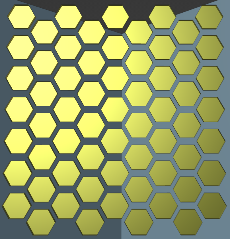
Figure 1: Reflector with hexagonal elements.

II-B Efficient Motor Control Design for Reflector Arrays

We design the reflector with $N_{c}$ columns, each comprising $N_{r}$ elements. In a simple design, each rotation requires the adjustment of a device, such as a motor. To control both horizontal and vertical orientations of each tile independently, two motors per tile would be required. Consequently, for a system with $N_{c}\times N_{r}$ elements, the total number of motors needed for full individual control would be $2\times N_{c}\times N_{r}$.

While independent control of all rotations is a simple design selection, it presents significant cost implications due to the large number of motors required. Therefore, our objective is to design a reflector system that strikes a balance between cost-effectiveness and beam-focusing performance requirements for real-world user activities. Therefore, the solution aims to reduce the total number of motors while maintaining sufficient flexibility to effectively manipulate signal paths in practical scenarios.

We propose a cost-effective yet performance-efficient approach for controlling reflector arrays. This strategy involves using one motor for the azimuth rotation ($\phi$) of each column while individual motors control the elevation rotation ($\theta$) of each tile. This design optimizes the trade-off between cost and performance efficiency.

Consider a reflector array with $N_{r}$ rows and $N_{c}$ columns serving $N_{K}$ users at diverse locations. Our motor control strategy is as follows:

• Elevation rotation ($\theta$): Individual motors control each tile.

• Azimuth rotation ($\phi$): One motor controls an entire column.

This approach enables beam-focusing for different users while significantly reducing the required number of motors. The total motor count is reduced to $(N_{r}+1)\times N_{c}$, representing a reduction factor of $\frac{2\times N_{r}\times N_{c}}{(N_{r}+1)\times N_{c}}=\frac{2\times N_{r}}{N_{r}+1}\approx 2$, compared to individual control of each unit. This strategy effectively balances cost-effectiveness and performance efficiency in practical deployments, allowing for scalable and flexible reflector array systems.

The proposed motor control strategy can be rationalized by conceptualizing the reflector array as a composite of vertically thin dish antennas. In this design, all tiles within a column form a cohesive group serving a specific purpose, such as focusing beams towards a particular user. This approach allows for uniform horizontal rotation within each column, as the reflection pattern for a column remains largely consistent. The strategy is particularly effective in real-world scenarios, where obstacles are often elongated in the vertical direction. When signals are obstructed by such vertically elongated objects, a column of reflective surfaces can easily adjust its azimuth rotation to mitigate interference.

Once a column achieves a suitable azimuth angle, individual tiles within the column can further optimize their elevation angles to focus beams precisely towards mobile users. This design effectively transforms each column into an independent thin-disk antenna capable of separate beam-focusing. By implementing this column-based control strategy, we significantly reduce the number of motors required while maintaining a high degree of flexibility for tile adjustment and beam-focusing. This approach not only optimizes cost-effectiveness, but also preserves high levels of performance, thus meeting the original design goals. The strategy strikes an optimal balance between motor reduction and performance optimization, ensuring an efficient and adaptable beam-focusing on various environmental conditions.

III System Model

This section outlines the core challenges addressed in our research and presents the wireless simulation framework employed to investigate our proposed solutions.

III-A Problem formulation

This research builds upon the concept of path gain improvement, as illustrated in [16] using controllable reflector, and applies it to more complex scenarios that include multiple transmit antennas, several users (a MU-MIMO system), and the presence of obstacles. The incorporation of multiple users and obstacles significantly increases the complexity of the optimization challenge.

In ideal conditions without obstacles, LOS paths exist between the AP, the reflector, and all users. However, the presence of obstacles creates a mixed scenario where some users maintain LOS with the reflector while others experience non-line-of-sight (NLOS) conditions, as illustrated in Figure 2. This heterogeneity in channel models among users substantially complicates the problem.

Our objective is to achieve autonomous operation of both the wireless communication system and the reflector. The wireless communication system functions largely independently of the reflector, providing only instantaneous performance feedback to the reflector controller. This approach maintains the conventional structure for uplink pilot transmission and downlink data transmission. The reflector operates strictly as an integral component of the wireless channel, without direct integration into the wireless communication system design. It relies solely on the received CSI from the wireless system to train models that learn environmental dynamics and determine optimal reflector configurations. This design enables the reflector to adapt to complex environments while minimizing modifications to existing wireless communication protocols.

In general, we aim to maximize the received power for all users under several constraints.

• Limited channel information, with only the receiver’s CSI known at the reflector.

• Presence of obstacles in the environment.

• Angular constraints on the movement of reflector elements.

Therefore, the optimization problem can be formulated as

—s— θ,ϕ∑_k=0^K G_k θ_i,j ∈[θ_min,θ_max],   ∀i ∈[1, …, N_r], j ∈[1, …, N_c] ϕ_j ∈[ϕ_min,ϕ_max],   ∀j ∈[1, …, N_c] , where $G_{k}$ is the measured path gain for user $k$. $\theta_{i,j}$ is the elevation angles of a unit in row $i$ and column $j$. $\phi_{j}$ is the azimuth angle of the column $j$. Equation (III-A) indicates the goal of maximizing the overall path gain for UE. Meanwhile, the constraints for tile rotation angles are presented in (III-A) and (III-A). In alignment with the ongoing development of a real-world experimental system, we define $\theta_{min}=\phi_{min}=-\frac{\pi}{4}$ and $\theta_{max}=\phi_{max}=\frac{\pi}{4}$.

To address the challenges associated with complex, multi-user environments that include obstacles, we propose utilizing DRL for reflector control. Our objective is to create a robust and adaptive solution that can optimize reflector configurations in dynamic settings marked by obstructions and multiple users. By leveraging DRL, the reflector can autonomously adjust its configuration based solely on feedback from CSI received from the user, rather than relying on CSI estimations for each tile of the reflector, which are extremely complex in real-world scenarios. This approach allows the system to respond effectively to the dynamic characteristics of wireless environments, accommodating obstacles and fluctuating channel conditions encountered by multiple users.

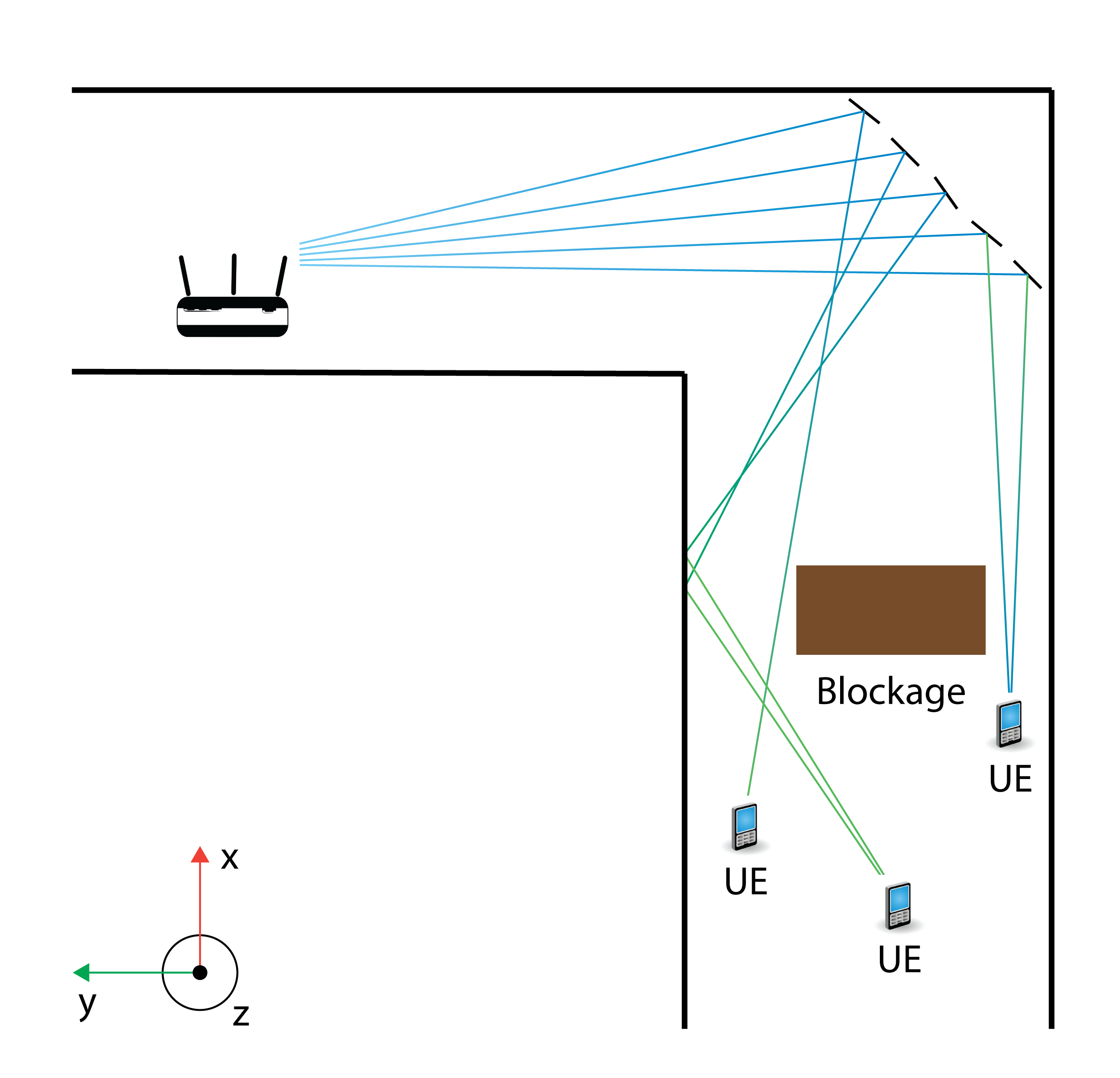
Figure 2: An example of an optimized reflector configuration to enhance signal quality for all UEs.

III-B Assumptions

We adopt a deterministic 3D ray-tracing approach to model the propagation of millimeter-wave signals. Ray tracing is well-suited for this frequency range because the dominant propagation mechanisms $-$ reflection, diffraction, and scattering $-$ closely resemble those encountered with optical wavelengths. By simulating multiple bounces off environmental objects until signal strength diminishes, our model captures the spatial and temporal characteristics essential for accurate high-frequency channel analysis.

We assume that when a ray encounters an object, it reflects specularly into the environment. Different materials have specific reflection coefficients, and each reflection diminishes signal power based on these coefficients, which depend on the ray’s direction and the surface material composition [28]. Furthermore, the ray-tracing method includes diffraction effects to improve simulation accuracy [29, 30].

To facilitate the simulation, several additional assumptions are made. First, it is assumed that all device positions are predetermined at the simulation’s outset, which is feasible in practical scenarios through the utilization of tracking technologies such as ultra-wideband (UWB) [31]. Furthermore, while constraints are imposed on the maximum and minimum angles of each tile, it is assumed that each tile of the reflector device can rotate continuously, enabling precise control over all tiles.

Additionally, it is assumed that there is a mechanism for UE to provide feedback on its measured channel condition to the reflector. This assumption is reasonable, as UEs perform channel estimation upon each signal reception. Moreover, given that UEs transmit their locations back to the reflector, the additional overhead required to send the receiver’s CSI to the reflector is likely to be minimal.

III-C Simulation Environment

We utilize NVIDIA Sionna as a compute engine for propagation calculations [32]. Sionna enables wireless simulations based on 3D models created with a modeling engine, specifically Blender [33] in our case. All materials are labeled according to the material list defined by Sionna. Figure 3 summarizes the workflow of this study.

NVIDIA Sionna utilizes ray tracing techniques to simulate signal propagation by reflecting rays off surfaces until either the maximum number of reflections is achieved or the ray no longer intersects any objects. This library calculates the electromagnetic characteristics of transmitted signals [34, 35], enabling the estimation of path loss through an analysis of these characteristics at UE.

Given that the ray tracing module of Sionna requires 3D models for simulation purposes, it is essential to create a 3D representation of the simulation environment. In this project, we leverage Blender’s modeling tools to incorporate structural elements such as walls, floors, ceilings, and a reflector with predefined configurations for orientation and element angles. The careful assignment of materials to each component of the 3D model is vital, as these materials greatly affect the reflection and transmission coefficients, which in turn influence the signal strength of users. Accurate modeling of these coefficients depends on the material properties, particularly their permittivity and conductivity.

To ensure the accuracy and reliability of our simulation, we conform to the guidelines established by the International Telecommunications Union (ITU) for specifying the relative permittivity and conductivity of all materials [28]. The ITU provides frequency-dependent constant values that enable the calculation of the real part of the relative permittivity, $\eta^{\prime}$, and conductivity, $\sigma$, for various material groups, derived from empirical measurement data. By incorporating these material properties, our simulation provides a realistic and accurate representation of the environment, enabling the evaluation of the reflector’s performance in a practical setting. Using the predefined constant values for each material, we calculate the material properties as follows.

$$\eta^{\prime}=af^{b},$$ (1)

$$\sigma=cf^{d},$$ (2)

where $\eta^{\prime}$ is dimensionless, $\sigma$ is in S/m, and $f$ is frequency in GHz. The values of $a,b,c$ and $d$ are measured constants for each material and are presented in I.

TABLE I: Material Properties.

Material	Metal	Concrete	Plaster	Ceiling
a	1	5.24	2.73	1.48
b	0	0	0	0
c	$10^{7}$	0.0462	0.0085	0.0011
d	0	0.7822	0.9395	1.0750
Frequency (GHz)	1-100	1-100	1 – 100	1 – 100

We accelerate the modeling and simulation process by developing a simulation pipeline that automates wireless signal calculations. The pipeline seamlessly transfers models between the Blender modeling engine and the Sionna compute engine. After setting up the default scene, the reflector’s configuration is adjusted using a Python API in Blender to calculate the rotation angles for the reflector array tiles. The configured 3D asset is then exported in XML format for wireless simulation.

IV Reflector Control with Deep Reinforcement Learning

IV-A Overview of Reflector Control with Deep Reinforcement Learning

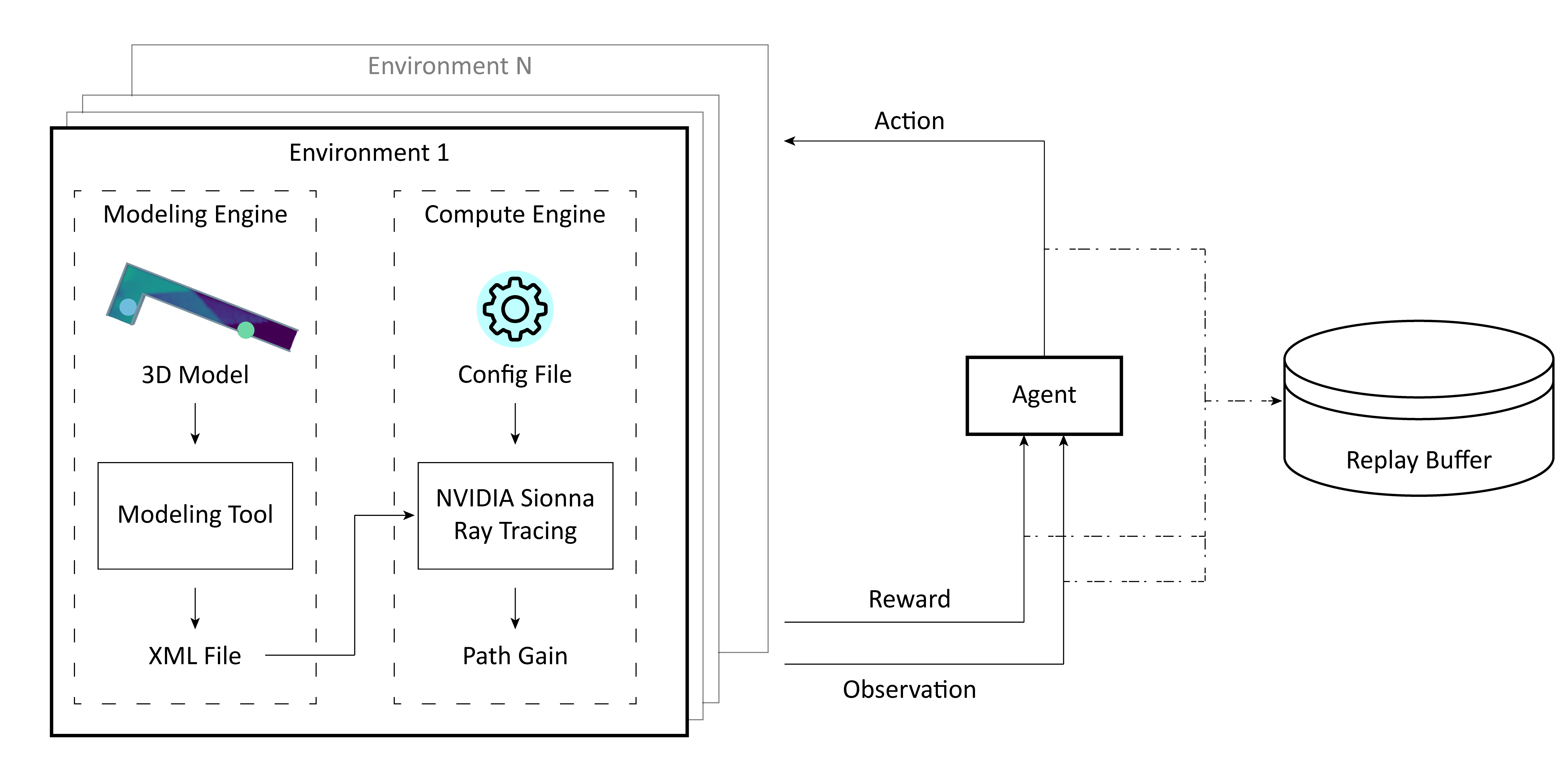
Figure 3: Workflow of the Deep Reinforcement Learning and the integrated environment with Sionna and Blender.

DRL frameworks employ an iterative learning paradigm in which an autonomous agent refines its behavioral patterns through interactions with its environment. Figure 3 illustrates this training process. The architecture of the learning system consists of several key components that enable the agent’s decision-making process.

IV-A1 Markov Decision Process (MDP)

The DRL framework is fundamentally structured as an MDP, characterized by the tuple $\pazocal{M}=(\pazocal{S},\pazocal{A},\pazocal{P},\pazocal{R},\gamma)$, where $\pazocal{S}$ represents the state space, $\pazocal{A}$ denotes the action space, $\pazocal{P}$ defines the state transition probability function, $\pazocal{R}$ specifies the reward function, and $\gamma\in(0,1]$ is the discount factor. Within this framework, at each timestep $t$, the agent observes the current state $s^{t}\in\pazocal{S}$, selects an action $a^{t}\in\pazocal{A}$ according to its policy $\pi$, receives a reward $r^{t}$, and transitions to a new state $s^{t+1}$ according to the probability distribution $\pazocal{P}(s^{t+1}|s^{t},a^{t})$. The objective is to learn an optimal policy $\pi^{*}$ that maximizes the expected cumulative discounted reward $\mathbb{E}\left[\sum_{t=0}^{\infty}\gamma^{t}r^{t}\right]$, where the discount factor $\gamma$ determines the trade-off between immediate and future rewards.

State: The state consists of three main components: (1) CSI of each UE, (2) rotation angles of all tiles, and (3) positions of all UEs.

The first component includes the CSI from all UEs. With $N_{K}$ UEs and $N_{T}$ AP antennas, the total dimension of the received CSI is $N_{K}\times N_{T}$.

We utilize both the real and imaginary components of the CSI as states of the DRL agent. This method is adopted to preserve both magnitude and delay information for all channel taps. By maintaining these distinct components, a more complete representation of channel characteristics is achieved, allowing a more comprehensive analysis of the signal propagation environment.

The second state component comprises the current rotation angles of the reflector tiles. These angles are defined within the angular space shown in (3). This representation provides a comprehensive description of the reflector’s current configuration, which is crucial for the system’s decision-making process.

$$s_{2}=\begin{bmatrix}\phi_{1,1}&...&\phi_{1,j}&...&\phi_{1,N_{c}}\\ \theta_{1,1}&...&\theta_{1,j}&...&\theta_{1,N_{c}}\\ \vdots&\ddots&\vdots&\ddots&\vdots\\ \theta_{i,1}&...&\theta_{i,j}&...&\theta_{i,N_{c}}\\ \vdots&\ddots&\vdots&\ddots&\vdots\\ \theta_{N_{r},1}&...&\theta_{N_{r},j}&...&\theta_{N_{r},N_{c}}\\ \end{bmatrix},$$ (3)

where, $\phi_{1,j}$ is the azimuth rotation of the $j^{th}$ column. $\theta_{i,j}$ is the elevation rotation of the $i^{th}$ row and the $j^{th}$ column. $N_{r}$ and $N_{c}$ are the number of rows and columns of the reflector elements, respectively.

The third set of states contains positions of all UEs, which are denoted as follows:

$$s_{3}=\begin{bmatrix}x_{\text{ue}_{1}}&y_{\text{ue}_{1}}&z_{\text{ue}_{1}}\\ \vdots&\vdots&\vdots\\ x_{\text{ue}_{K}}&y_{\text{ue}_{K}}&z_{\text{ue}_{K}}\\ \end{bmatrix},$$ (4)

where $K$ is the number of UEs.

Action: We develop an action space for DRL based on the reflector structure, where all elements in a column share the same azimuth rotation but have individual elevation rotations. Utilizing all rotation angles would create an excessively large action space, potentially causing training divergence or prolonging the process. To address this, we implement a technique to reduce the action space, as illustrated in Figure 4. By treating each column as a thin disk antenna, we use a focal point to manage the angular movement of the tiles.

To ensure compliance with physical constraints on angular rotation, we perform a transformation from Cartesian to spherical coordinates, facilitating the imposition of angular limits during training. Consequently, we define control values for each column, including azimuth rotation (angle $\phi$), elevation rotation of the middle element (angle $\theta$), and a point along the normal vector of the middle element with a distance of $R$. This design reduces the action space by $\nicefrac{{(1+N)}}{{3}}$, significantly lowering its dimensionality and expediting DRL agent training.

Based on the aforementioned concept, the action space is defined as follows.

$$a=\begin{bmatrix}\Delta\phi_{1}&...&\Delta\phi_{j}&...&\Delta\phi_{N_{c}}\\ \Delta\theta_{1}&...&\Delta\theta_{j}&...&\Delta\theta_{N_{c}}\\ \Delta R_{1}&...&\Delta R_{j}&...&\Delta R_{N_{c}}\\ \end{bmatrix},$$ (5)

where $\Delta\phi_{j}$ represents the change in the azimuth rotation angle, $\Delta\theta_{j}$ denotes the change in the elevation rotation angle for the middle tile, and $\Delta R_{j}$ indicates the change in distance of a point along the normal vector of the middle tile from that tile. The subscript $j$ refers to the $j^{\text{th}}$ column.

To employ the new action space design to control the reflector’s elements, a conversion process is required to adjust all elements within a column based on the middle element’s configuration, specified by $\phi$, $\theta$, and $R$. The goal is to align all elements towards the point $R$, effectively creating a thin disk antenna. This requires that the normal vectors of all elements point towards $R$.

The movement of the focal point $R$ induces a rotation of all elements in the column to face point $R$. This approach is based on the assumption that UE are generally not co-located in the x-y plane but are significantly separated in the z-direction, implying that two or more users cannot occupy the same x-y location while differing substantially in altitude.

Once the point $R$ is established, the rotation angles for all other tiles can be computed. This is achieved by aligning the normal vectors of all tiles to point towards $R$. Subsequently, after obtaining the correct normal vectors for all tiles, the rotation angles can be calculated using the standard transformation from the Cartesian coordinate system to the spherical coordinate system. This transformation enables the determination of both angles, $\theta$ and $\phi$, utilizing equations (6), (7), and (8).

$$r=\sqrt{x^{2}+y^{2}+z^{2}}\text{,}$$ (6)

$$\theta=\arccos\left(\dfrac{z}{r}\right)\text{,}$$ (7)

$$\phi=\text{atan2}\left(\dfrac{y}{x}\right)\text{,}$$ (8)

where $x$, $y$, and $z$ are Cartesian coordinates of the normal $\vec{n}$, $r$ is the length of the normal $\vec{n}$, $\theta$ is the elevation angle, $\phi$ is the azimuth angle, atan2 is the 2-argument arctangent.

(a) Simple Design.

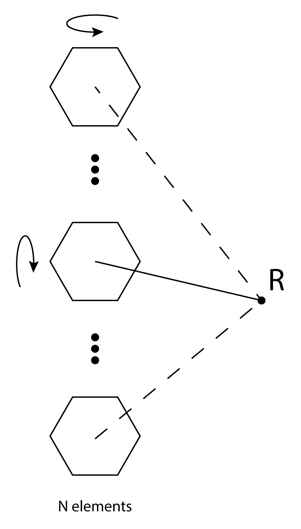
(b) Improved Design.

Figure 4: Reflector design for action space of Deep Reinforcement Learning agent. (a) Simple design with 1 + N control values per column. (b) Improved design with 3 control values per column.

Reward: The reward function is formulated to accelerate the training process of the agent. This is accomplished through an informative reward function that allows the agent to distinguish between favorable and unfavorable actions based on its current observation. The reward function relies on information derived from the agent’s present observation and action, specifically the path gain at the current time step and the path gain at the previous time step. After gathering the path gains for all users, these values, expressed in decibels, are subjected to the following processing steps.

Initially, path gains of all users are averaged out.

$$G_{avg}^{t}=\frac{1}{K}\sum_{k=0}^{K}G_{k}^{t},$$ (9)

where $G_{k}$ is the path gain of user $k$.

Subsequently, the average path gain is adjusted by a piece-wise function shown in (10), with a transition point determined to be a threshold gain. This threshold, which depends on the given environment, is informed by observations showing that a large, single flat reflector (serving as a baseline) positioned at the same location typically achieves an average path gain of approximately $-85$ dB. Using DRL, our goal is to exceed this baseline and enhance the average path gains for all users.

$$G_{adj}^{t}(G_{avg}^{t})=\begin{dcases}\frac{G_{avg}^{t}+G_{th}}{c_{1}},&G_{avg}^{t}<G_{th}\\ \frac{G_{avg}^{t}+G_{th}}{c_{2}}+c_{r},&\text{otherwise}\end{dcases}$$ (10)

where $G_{adj}$ represents the adjusted gain for this scenario. $G_{th}$ represents a path gain threshold used to evaluate whether the configuration achieves good performance. In our implementation, we set $G_{th}=-82.5$ dB. This value is chosen to be higher than the baseline’s average path gain of $-85$ dB, ensuring our agent achieves superior performance. The scaling factors $c_{1}$ and $c_{2}$ are set to $10$ and $5$, respectively. Additionally, when the average gain $G_{avg}$ surpasses the threshold $G_{th}$, an extra reward constant $c_{r}$, empirically determined to be $1.5$, is applied. These parameter values are chosen to enhance the agent’s learning process.

The reward is also dependent on the path gain information of the previous observation as we can evaluate how good the taken action is. The difference between path gains of the current step and previous are added to the reward.

$$G_{diff}^{t}=\frac{1}{K}\sum_{k=0}^{K}(G_{k}^{t}-G_{k}^{t-1}),$$ (11)

where $G_{i}^{t}$ and $G_{i}^{t+1}$ are the path gain in dB of user $k$ at time step $t$ and $t+1$, respectively.

Additionally, the agent receives a penalty when executing actions that result in out-of-bounds rotational movements at the angular limits of the system. This boundary constraint mechanism helps enforce operational limits and encourages the agent to maintain movements within the physical range of motion.

$$C=\begin{dcases}1,&\text{for each violation}\\ 0,&\text{otherwise}\end{dcases}$$ (12)

Finally, the reward for each step is defined based on the current state of the agent as well as the action the agent takes. Particularly, it is defined as follows:

$$\pazocal{R}^{t}(s^{t},a^{t},s^{t+1})=G_{adj}^{t}+w_{1}\times G_{diff}^{t}-w_{2}\times C,$$ (13)

where $w_{1}$ and $w_{2}$ represent weighting coefficients for $G_{diff}$ and $C$, set to $0.03$ and $0.3$, respectively. These coefficients are carefully calibrated to ensure appropriate balance between different terms, optimizing the agent’s overall performance.

IV-A2 Policy

The policy $\pi(a^{t}|s^{t})$ defines the probability distribution over actions $a^{t}$ conditioned on the current state $s^{t}$. This stochastic mapping satisfies the probability constraint:

$$\sum_{a^{t}\in A}\pi(a^{t}|s^{t})=1.$$ (14)

IV-A3 State-Action Value Function

The state-action value function $Q_{\pi}(s^{t},a^{t})$ quantifies the expected cumulative discounted reward when executing action $a^{t}$ in state $s^{t}$ and following policy $\pi$ thereafter. This is formally expressed as:

$$Q_{\pi}(s^{t},a^{t})=\mathbb{E}_{\pi}[r^{t}|s^{t}=s,a^{t}=a],$$ (15)

where the return $r^{t}$ is defined as:

$$r^{t}=\sum_{\tau=0}^{\infty}\gamma^{\tau}r^{(t+\tau+1)},$$ (16)

with discount factor $\gamma\in(0,1]$.

IV-A4 Bellman Equation

The Q-function adheres to the Bellman equation:

$$Q_{\pi}(s^{t},a^{t}) =\mathbb{E}_{\pi}[r^{t+1}|s^{t}=s,a^{t}=a]$$ (17)

$$+\gamma\sum_{s^{\prime}\in S}P_{ss^{\prime}}^{a}\left(\sum_{a^{\prime}\in A}\pi(s^{\prime},a^{\prime})Q^{\pi}(s^{\prime},a^{\prime})\right),$$

where $P_{ss^{\prime}}^{a}=\pazocal{P}(s^{t+1}|s^{t},a^{t})$ represents the transition probability to state $s^{\prime}$ given the current state-action pair $(s,a)$.

IV-A5 Experience Definition

The experience tuple $(s^{t},a^{t},r^{t+1},s^{t+1})$ encapsulates a single interaction step, comprising the current state $s^{t}$, action taken $a^{t}$, resulting reward $r^{t+1}$, and subsequent state $s^{t+1}$. This formulation enables the agent to learn from historical interactions and update its policy accordingly.

IV-B Soft Actor-Critic Algorithms

IV-B1 Algorithm Description

In this study, we employ the Soft Actor-Critic (SAC) algorithm to optimize the reflector configuration. SAC, an off-policy algorithm, introduces entropy maximization to enhance exploration and improve robustness. It learns a stochastic policy by maximizing both the expected return and the policy’s entropy, thereby preventing premature convergence to suboptimal solutions [36, 37].

The SAC algorithm offers several key advantages in reinforcement learning. Its entropy maximization approach facilitates efficient exploration of the state-action space, enhancing the algorithm’s ability to discover optimal policies. SAC also demonstrates greater robustness across diverse tasks compared to deterministic methods like Deep Deterministic Policy Gradient (DDPG) [38] and Twin-Delayed Deep Deterministic (TD3) [39], making it more adaptable to various domains. Additionally, its temperature adjustment mechanism allows for a fine-tuned balance between exploration and exploitation during learning. These features make SAC well-suited for optimizing reflector configurations in dynamic, multi-user wireless environments with obstacles. Moreover, given that it takes approximately 4 seconds for each step on a NVIDIA 3090 GPU, the use of off-policy algorithms like SAC is advantageous, ruling out on-policy methods such as Proximal policy optimization (PPO) [40].

To be more precise, SAC is an actor-critic algorithm that aims to learn a policy by optimizing both the expected return and entropy for each state encountered in a trajectory.

$$\pi^{*}=\arg\max_{\pi}\sum_{t}\mathop{\mathbb{E}}_{(s^{t},a^{t})\sim\rho_{\pi}}\left[r(s^{t},a^{t})+\alpha\pazocal{H}(\pi(\cdot|s^{t}))\right],$$ (18)

where $\pazocal{H}(\pi(a|s))=\mathop{\mathbb{E}}_{a\sim\pi}[-\text{log}\pi(a|s)]$ is the entropy. $\alpha$ is the temperature parameter that controls the trade-off between entropy and reward.

This process is achieved through soft-policy iteration, which involves repeatedly applying the entropy-augmented (soft) Bellman operator.

$$Q(s^{t},a^{t})=r_{t}+\gamma\mathop{\mathbb{E}}_{s^{t+1}\sim p}\left[V(s^{t+1})\right],$$ (19)

where

$$V(s^{t+1}) =\mathop{\mathbb{E}}_{a^{t+1}\sim\pi}\left[Q(s^{t+1},a^{t+1})-\alpha\log\pi(a^{t+1}|s^{t+1})\right].$$ (20)

We employ function approximators for both the soft Q-function and the policy. We alternate between optimizing both networks using stochastic gradient descent. Specifically, we parameterize the soft Q-function as $Q_{\xi}(s^{t},a^{t})$ and the policy as $\pi_{\psi}(a^{t}\mid s^{t})$, where $\xi$ and $\psi$ represent the respective parameters of these networks. For instance, the soft Q-function can be represented by expressive neural networks, while the policy can be modeled as a Gaussian distribution, with its mean and covariance determined by neural networks. The parameters of the soft Q-function can be optimized by minimizing the soft Bellman residual.

$$J_{Q}(\xi)=\mathop{\mathbb{E}}_{(s^{t},a^{t})\sim\pazocal{D}}\left[\frac{1}{2}\left(Q_{\xi}(s^{t},a^{t})-Q_{\text{target}}\right)^{2}\right],$$ (21)

where

$$Q_{\text{target}}=r(s^{t},a^{t})+\gamma\mathop{\mathbb{E}}_{s^{t+1}\sim p}[V_{\xi^{\prime}}(s^{t+1})],$$ (22)

where the value function is implicitly based on the soft Q-function parameters defined in (20) and uses a target soft Q-function with parameters $\xi^{\prime}$ updated by an exponential moving average, ensuring smoother and more stable learning.

The policy parameters $\psi$ can be optimized by directly minimizing the expected Kullback-Leibler (KL) divergence between the policy distribution and the exponential of the Q-function. This minimization process effectively learns the optimal policy by reducing the probabilistic distance between the policy’s action distribution and the distribution implied by the value function.

$$J_{\pi}(\psi)=\mathop{\mathbb{E}}_{s^{t}\sim\pazocal{D}}\left[\mathop{\mathbb{E}}_{a^{t}\sim\pi_{\psi}}\left[\alpha\log(\pi_{\psi}(a^{t}|s^{t}))-Q_{\xi}(s^{t},s^{t})\right]\right].$$ (23)

This formulation allows for direct optimization of the policy parameters through gradient descent methods, where the objective function $J_{\pi(\psi)}$ captures both the entropy of the policy (through the log term) and the expected value of actions (through the soft Q-function).

In our approach, the Q-function, used to evaluate how good an action is in a given state, is represented as a differentiable neural network. To train this network more efficiently, we apply the reparameterization trick instead of sampling actions directly from the policy’s probability distribution. This trick involves generating a noise sample from a simple distribution and then using a deterministic function of both this noise and the network parameters to produce an action. By shifting randomness into the noise sampling step, we can calculate gradients more reliably, which ultimately reduces the variance of our gradient estimates and stabilizes training.

$$a^{t}=f_{\psi}(\epsilon^{t};s^{t}),$$ (24)

where, the noise vector $\epsilon^{t}$ represents a random input that is drawn from a predefined probability distribution, with a common choice being a spherical (isotropic) Gaussian distribution $\epsilon^{t}\sim\pazocal{N}(\mathbf{0},\mathbf{I})$.

The final objective of the policy is then as follows:

$$J_{\pi}(\psi)= \mathop{\mathbb{E}}_{s^{t}\sim\pazocal{D},\epsilon^{t}\sim\pazocal{N}}[\alpha\log\pi_{\psi}(f_{\psi}(\epsilon^{t};s^{t})|s^{t})$$ (25)

$$\quad\quad\quad\quad\quad-Q_{\xi}(s^{t},f_{\psi}(\epsilon^{t};s^{t}))],$$

where $\pi_{\psi}$ is defined implicitly in terms of $f_{\psi}$. $a^{t}$ is evaluated at $f_{\psi}(\epsilon^{t};s^{t})$.

IV-B2 Dual Critic Architecture

The framework implements dual critic networks to alleviate the overestimation of action values [39]. Critic networks are parameterized by $\xi_{1}$ and $\xi_{2}$ to evaluate action values:

$$Q_{\xi_{i}}(s,a),\quad i\in\{1,2\}.$$ (26)

Each critic is paired with a target network ($\xi_{1}^{\prime}$, $\xi_{2}^{\prime}$):

$$Q_{\xi_{i}^{\prime}}(s,a),\quad i\in\{1,2\}.$$ (27)

The target networks use soft updates, shown in (28), to maintain a slowly-moving average of the critics’ parameters. This dual-network architecture mitigates value overestimation through ensemble estimation while enhancing training stability through complementary value function approximation.

$$\xi_{i}^{\prime}\leftarrow(1-\tau)\xi_{i}^{\prime}+\tau\xi_{i},\quad i\in\{1,2\},$$ (28)

where $\tau$ is the smoothing factor, $0<\tau<1$. A smaller value of $\tau$ results in slower updates, providing more stability.

IV-C Neural Network Design

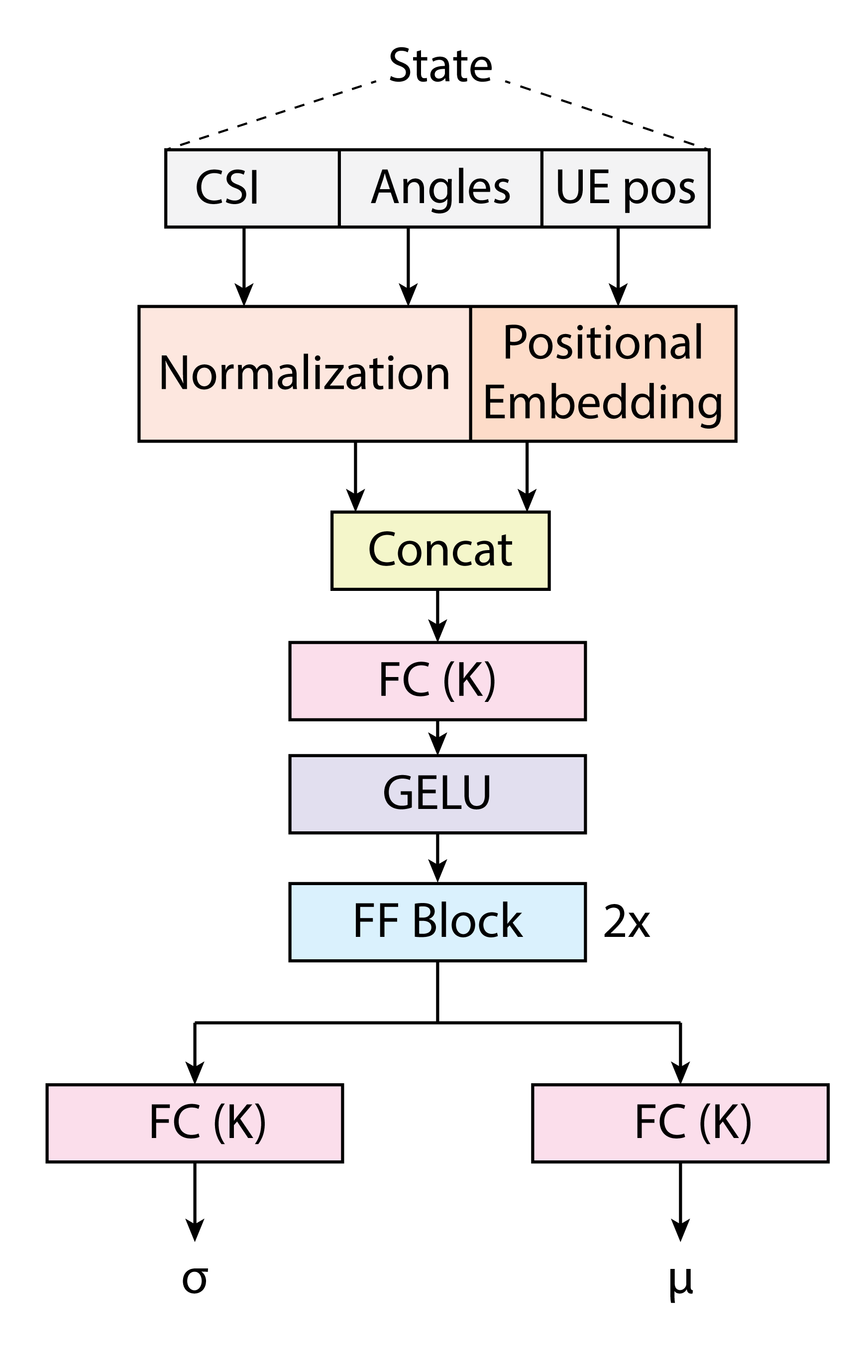
(a)

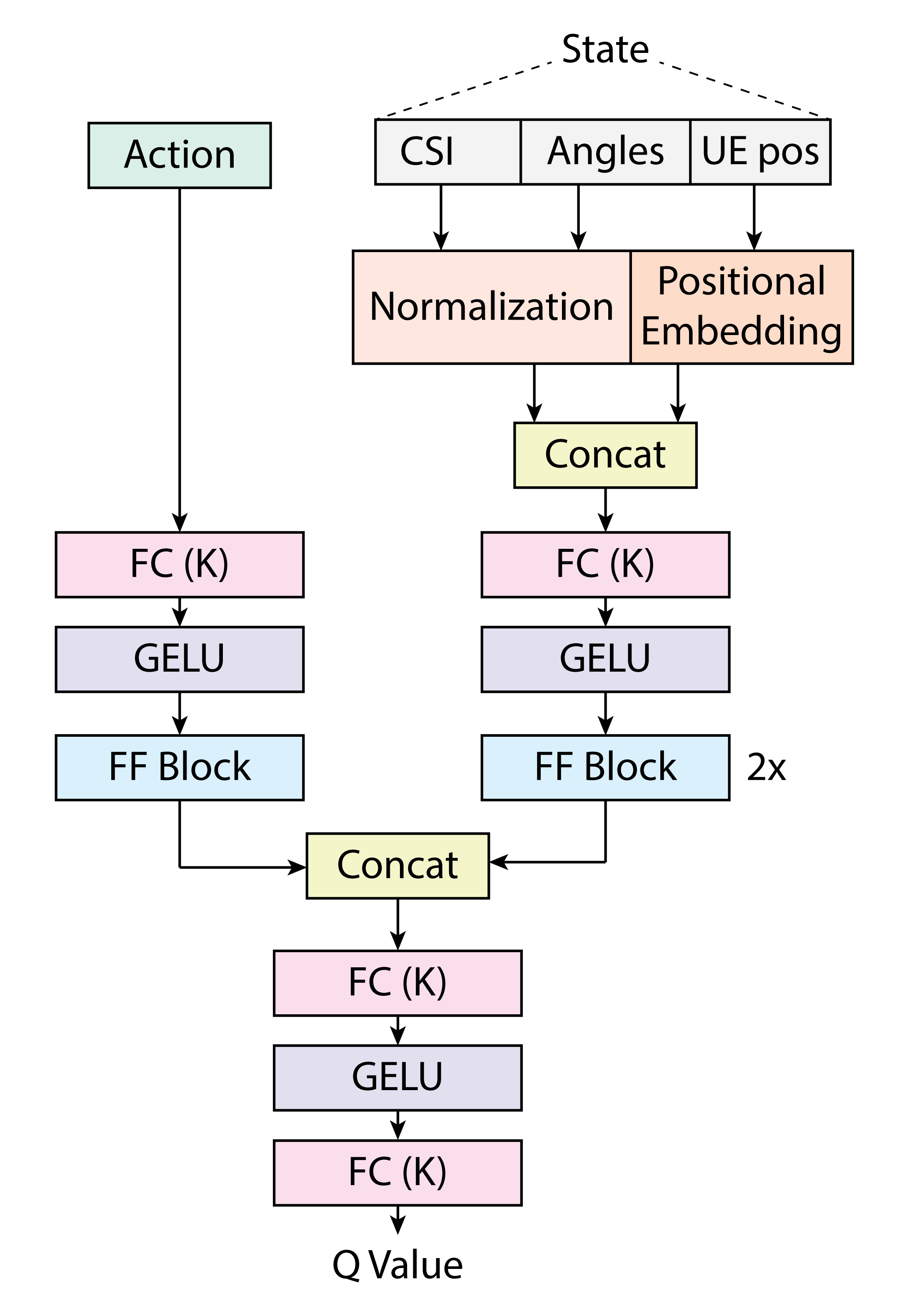
(b)

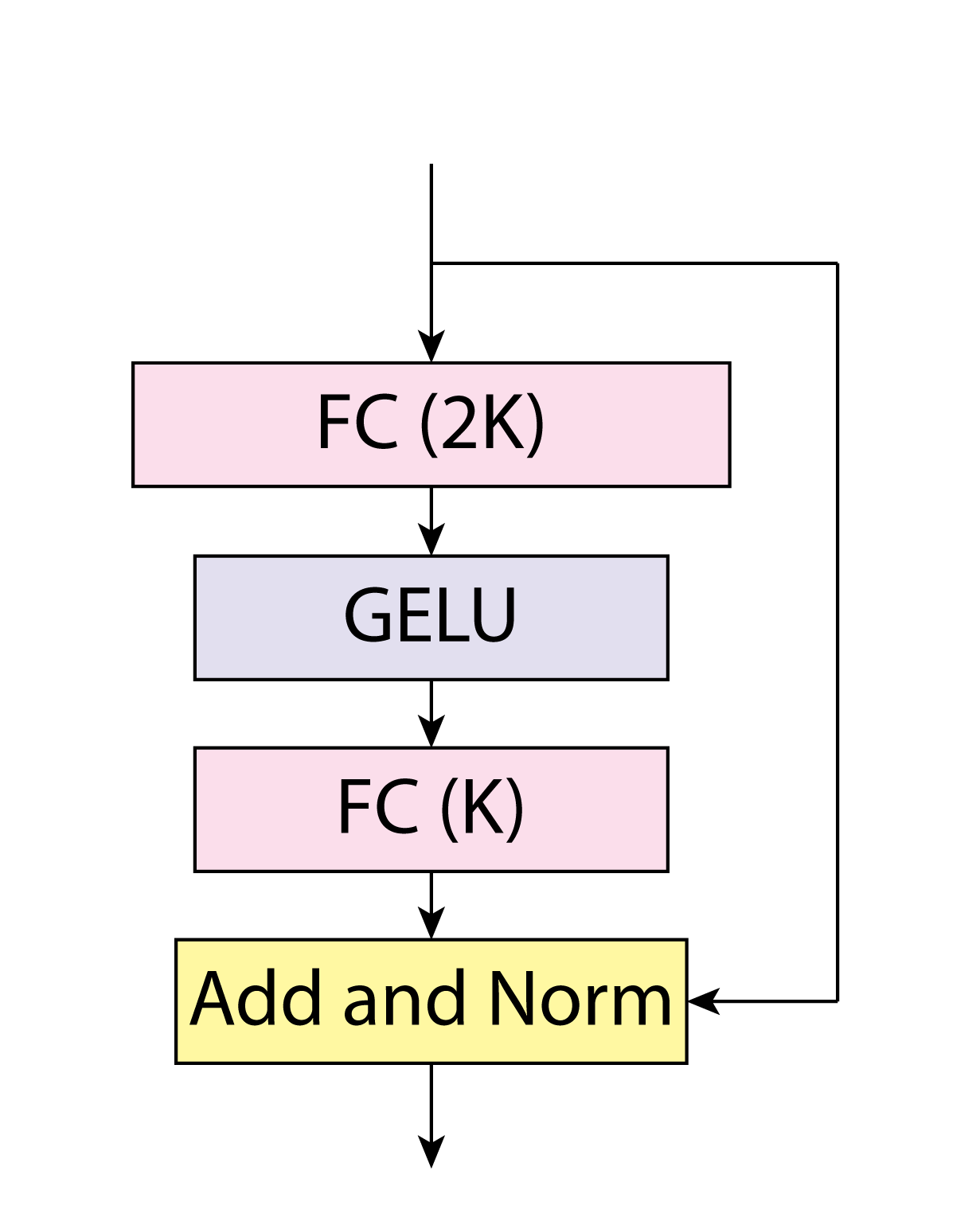
(c)

Figure 5: Neural network architectures of actor and critic.

IV-C1 Embedding Position

Positional embedding in Neural Radiance Fields (NeRF) [41, 42] is a method that transforms low-dimensional input coordinates into a higher-dimensional feature space using periodic trigonometric functions. By applying sine and cosine transformations to spatial coordinates and viewing directions, this technique addresses the spectral bias of neural networks, enabling more detailed representation of complex geometric and appearance variations. The frequency-based encoding enhances the network’s capacity to represent details, allowing for efficient capture of high-frequency scene features with minimal computational overhead. In our implementation, this encoding is used to map user positions into a higher-dimensional feature space, thereby accelerating the training of the agent.

IV-C2 Critic Network

The architecture incorporates a feed-forward block augmented with a residual connection as shown in Figure 5(c), a design choice that substantially enhances the training efficacy of the neural network. This approach, which facilitates improved gradient flow and mitigates the vanishing gradient problem, has been demonstrated to be particularly effective for large language models [43].

The architecture of the critic network is depicted in Figure 5(b). The network processes a state vector comprising UE positions, reflector angles, and CSI. Prior to input, the state undergoes preprocessing: CSI is normalized using the sample mean and variance, while angles are scaled to the range $[-\nicefrac{{\pi}}{{4}},\nicefrac{{\pi}}{{4}}]$. This preprocessed state representation is then propagated through a series of fully connected layers and feed-forward blocks, each containing $K$ neurons.

Concurrently, the action vector is processed through multiple fully connected layers, also with $K$ neurons. The critic network ultimately generates a Q-value for the given state-action pair. This Q-value serves as the output of the network, providing a measure of the expected cumulative reward for the input state and action combination.

IV-C3 Actor Network

The actor network’s architecture is similar to that of the critic network, employing a combination of fully connected layers and feed-forward blocks, as illustrated in Figure 5(a). However, the actor network’s output two key parameters: the mean and variance of the action distribution. These outputs characterize the probabilistic nature of the actor’s policy, enabling the network to model a continuous action space and facilitate exploration during the learning process. During the evaluation process, the output mean is used as action of the DRL agent.

V Results and Discussion

This section assesses the reflector’s effectiveness in enhancing wireless signal reception for multiple users in NLOS conditions. We evaluate our DRL-based optimization approach for beam allocation and path gain maximization for different experiments. The analysis focuses on downlink transmission performance with an AP operating at 28 GHz.

V-A Hyperparameters

The hyperparameters used in this study are outlined in Table II. The optimization process involves extensive parameter tuning, requiring numerous iterations to obtain values that reflect meaningful agent learning behavior. Each experimental iteration requires approximately 24 hours to establish distinct learning trajectories or significant performance indicators, primarily due to the slow simulation speed of 4 seconds per sample on a single NVIDIA 3090 GPU. This thorough optimization process can be accelerated by employing parallel computing resources.

TABLE II: SAC Hyperparameters.

Parameter	Value
number of neurons (K)	256
optimizer	AdamW
critic learning rate	4.0 $\cdot 10^{-4}$
actor learning rate	1.8 $\cdot 10^{-4}$
learning rate schedule	constant
discount ($\gamma$)	0.985
replay buffer size	3 $\cdot 10^{4}$
minibatch size	256
non-linearity	GELU
entropy coefficient ($\alpha$)	auto
target entropy	$-\dim(\pazocal{A})$
target smoothing coefficient ($\tau$)	0.005
train frequency	episodic
warm-up steps prior to learning	1 001

V-B Downlink Transmission in an L-shaped Hallway with Fixed User Positions

Figure 6: Episodic return during training for the scenario with fixed user positions. The solid line is the mean of episodic return for many different runs, while the shaded area is the variance.

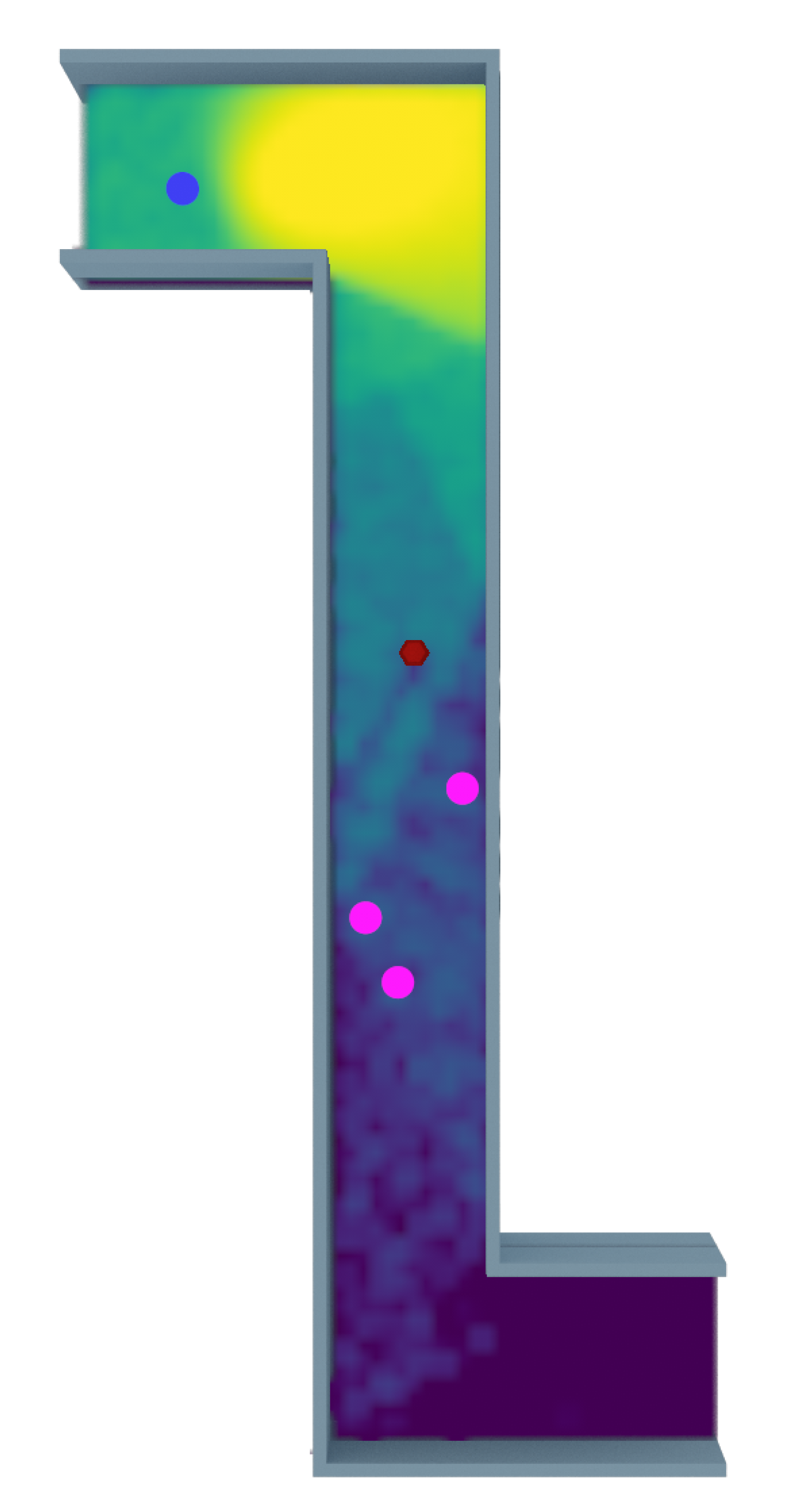
(a)

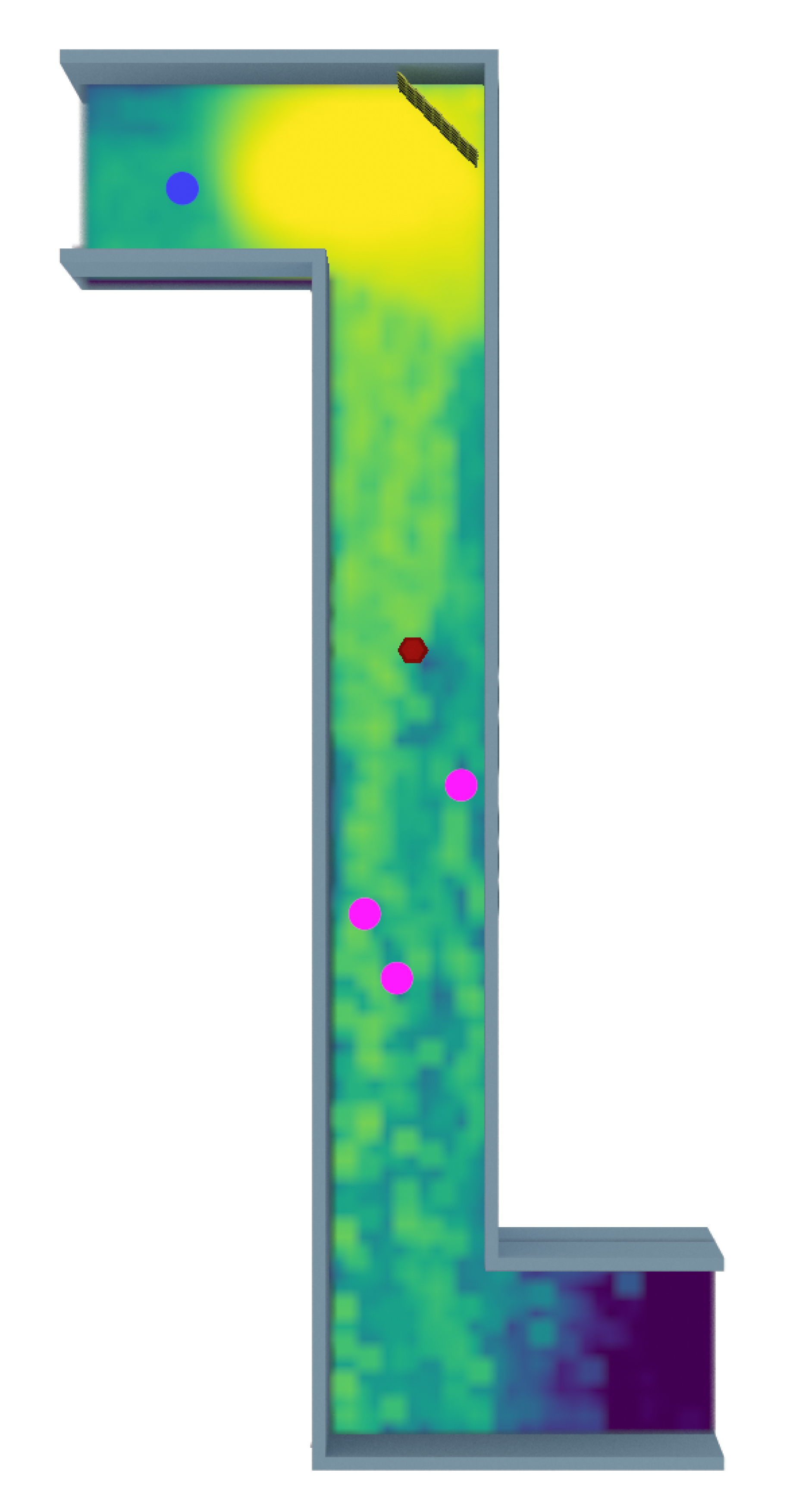
(b)

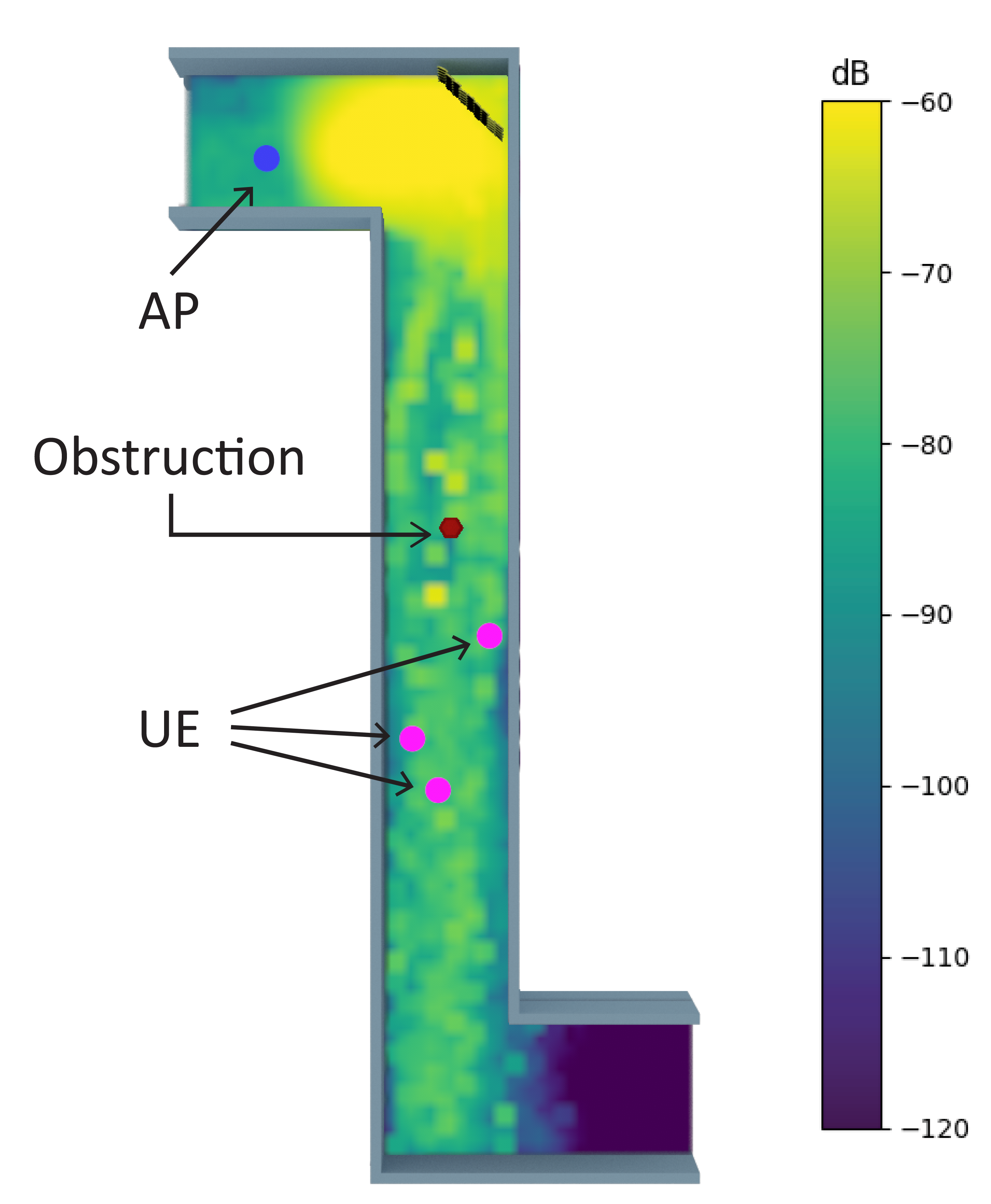
(c)

Figure 7: Path Gain for different scenarios. The Access Point (AP) is depicted in blue, while the users are shown in pink. The obstruction is represented in red.

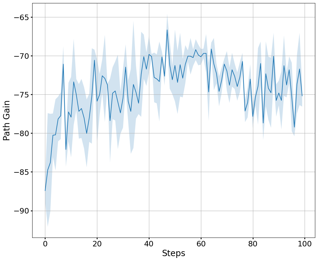
Figure 8: Evaluation results for fixed user positions in an L-shaped hallway.

Experiments conducted in an L-shaped hallway investigate wireless signal propagation in the presence of obstacles. The experimental setup includes fixed positions for the AP and UE, with a reflector located at the corner of the hallway. The AP has four antennas, while each UE has one antenna. The indoor environment is constructed with plasterboard walls, a ceiling board, a concrete floor, and wooden furniture as obstruction.

To simulate real-world conditions, the initial configuration of the reflector is randomized within physical constraints at the beginning of each episode. This approach mimics practical scenarios where reflector tile angles may exhibit diverse configurations prior to focusing signal beams towards designated users.

Figure 6 demonstrates the DRL-based algorithm’s adaptability, showing its ability to optimize reflector configurations by learning from the environment. The training process iteratively enhances signal propagation efficiency, enabling the system to autonomously determine optimal tile orientations for maximizing user signal strength, regardless of initial reflector conditions.

The effectiveness of the proposed approach is also evaluated through an analysis of path gains achieved by the optimized reflector configuration against two baseline setups. The first baseline scenario is characterized by the absence of any reflector (Figure 7(a)), while the second baseline incorporates a large flat metal surface positioned at the corner of the hallway (Figure 7(b)).

Figure 7 shows significant difference in performance across the different configurations. In the first baseline scenario without a reflector, the average path gain across all users is measured at $-105.126$ dB. The introduction of a large flat metal surface in the second baseline scenario yields an improved average path gain of $-87.233$ dB. In contrast, a controllable reflector system made up of multiple small tiles, autonomously controlled by DRL, shows a significantly improved average path gain of around $-75$ dB (Figure 7(c)).

After the training phase, this system is evaluated across various runs with different initial tile configurations. Despite these varying starting conditions, the DRL-based reflector effectively reconfigures its tiles over several iterations to optimize the average path gain for all users. It consistently achieves and maintains an average path gain of approximately and above $-75$ dB throughout the evaluation period (Figure 8). This improvement in signal propagation highlights the potential of DRL-based reflector configurations to enhance wireless communication systems. Video results of all evaluation runs of the study can be found at [44].

The substantial performance gap between the DRL-controlled reflector and the baseline scenarios highlights the effectiveness of the proposed approach. By leveraging the adaptability and fine-tuned control offered by the DRL algorithm, the system demonstrates its ability to optimize signal propagation in an obstructed environment, potentially enhancing wireless communication in indoor environments.

V-C L-shaped Hallway with Randomized User Positions

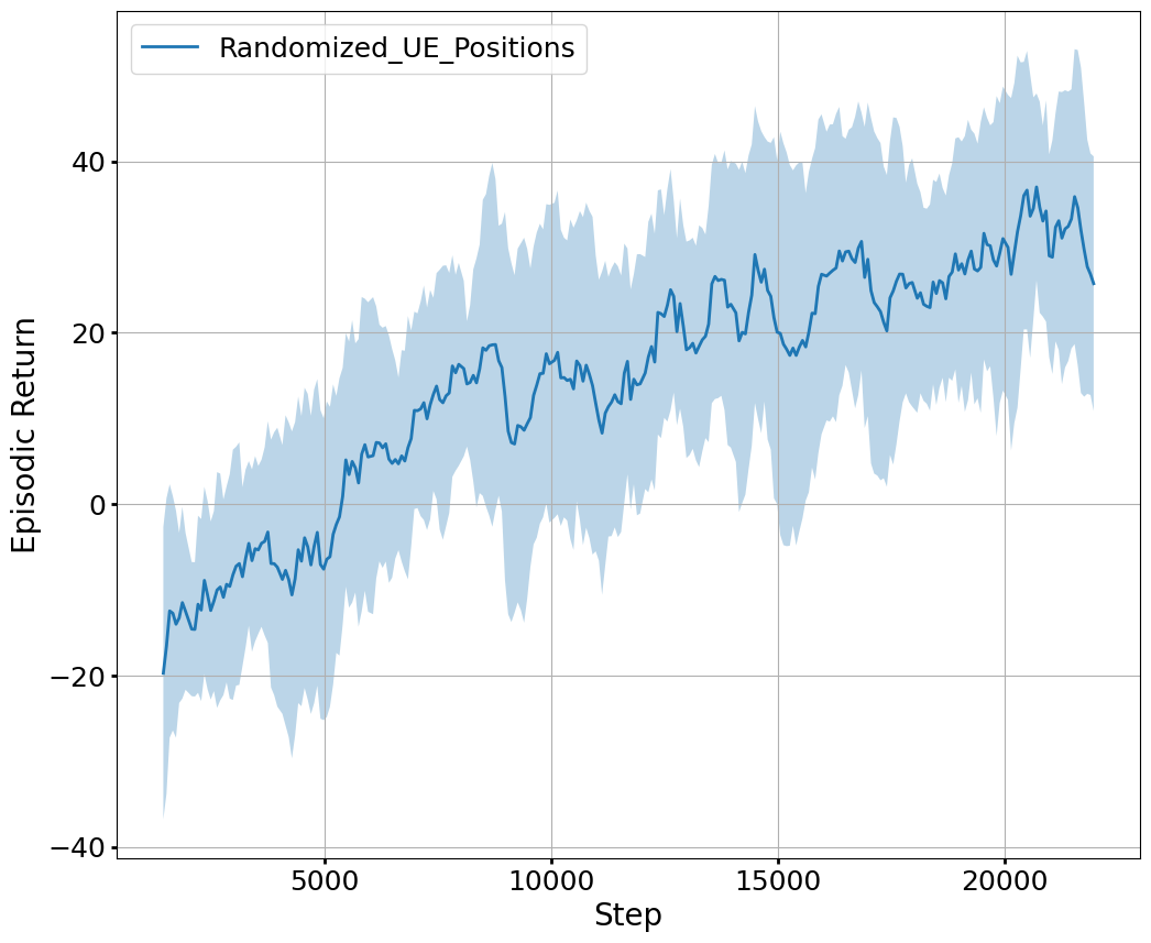
Figure 9: Episodic return during training for the scenario with randomized user positions.

Figure 10: Average path gain across all users for different evaluation runs.

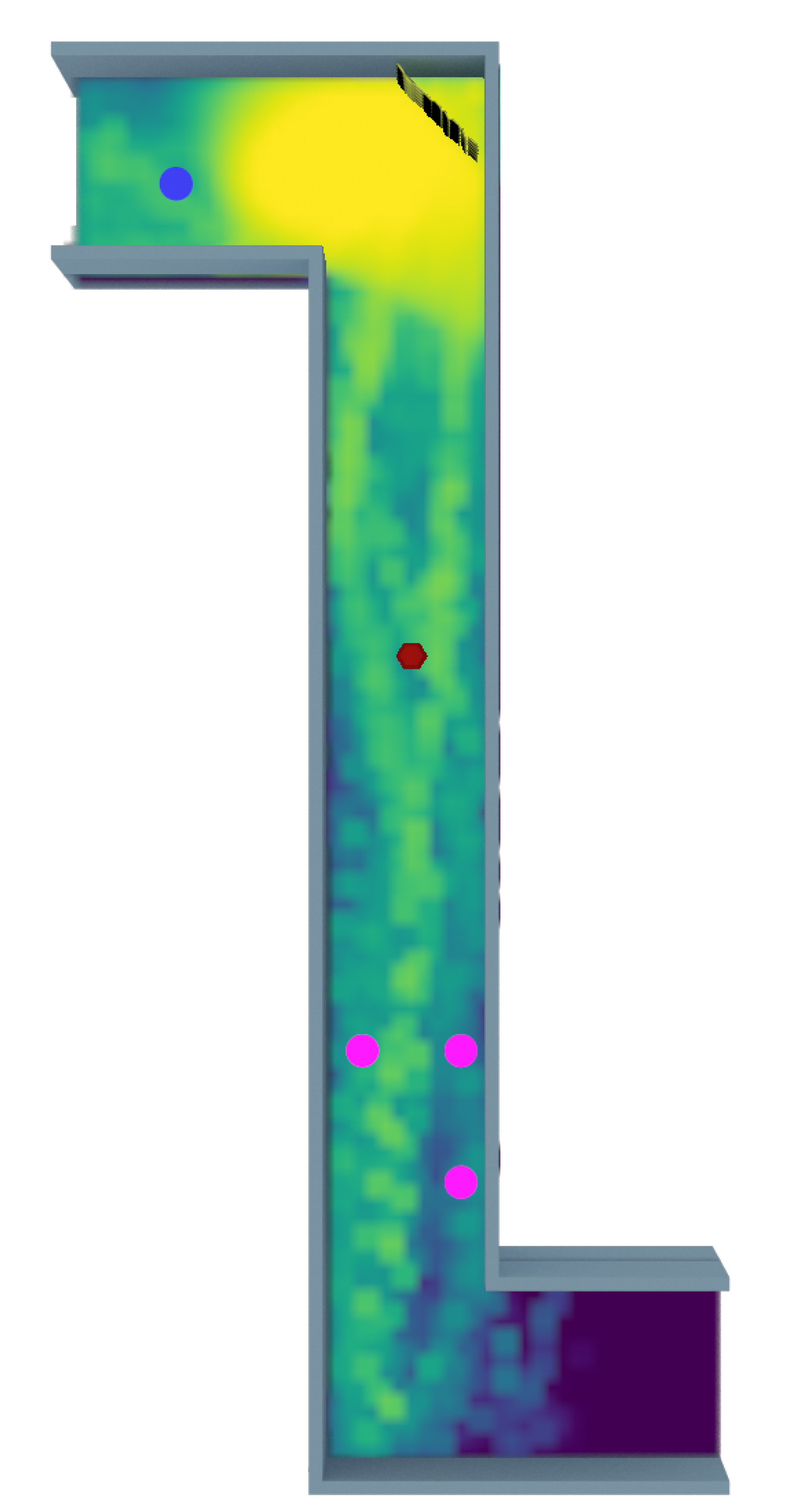
(a)

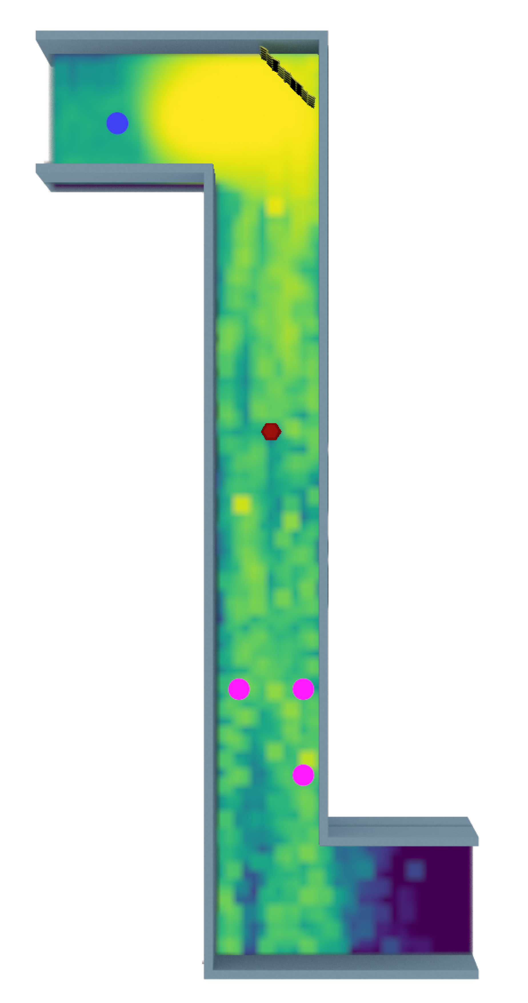
(b)

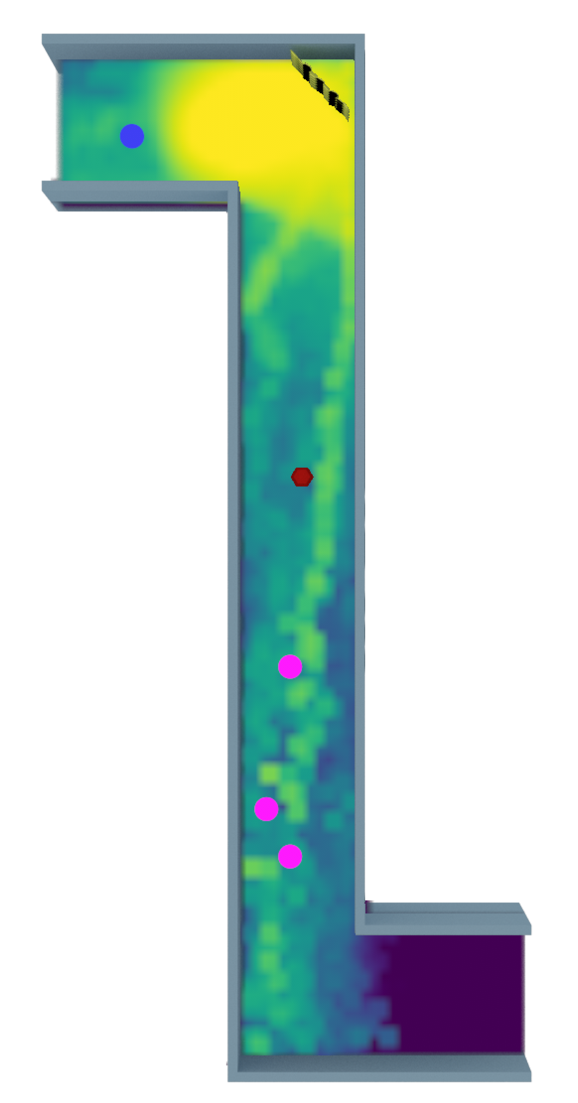
(c)

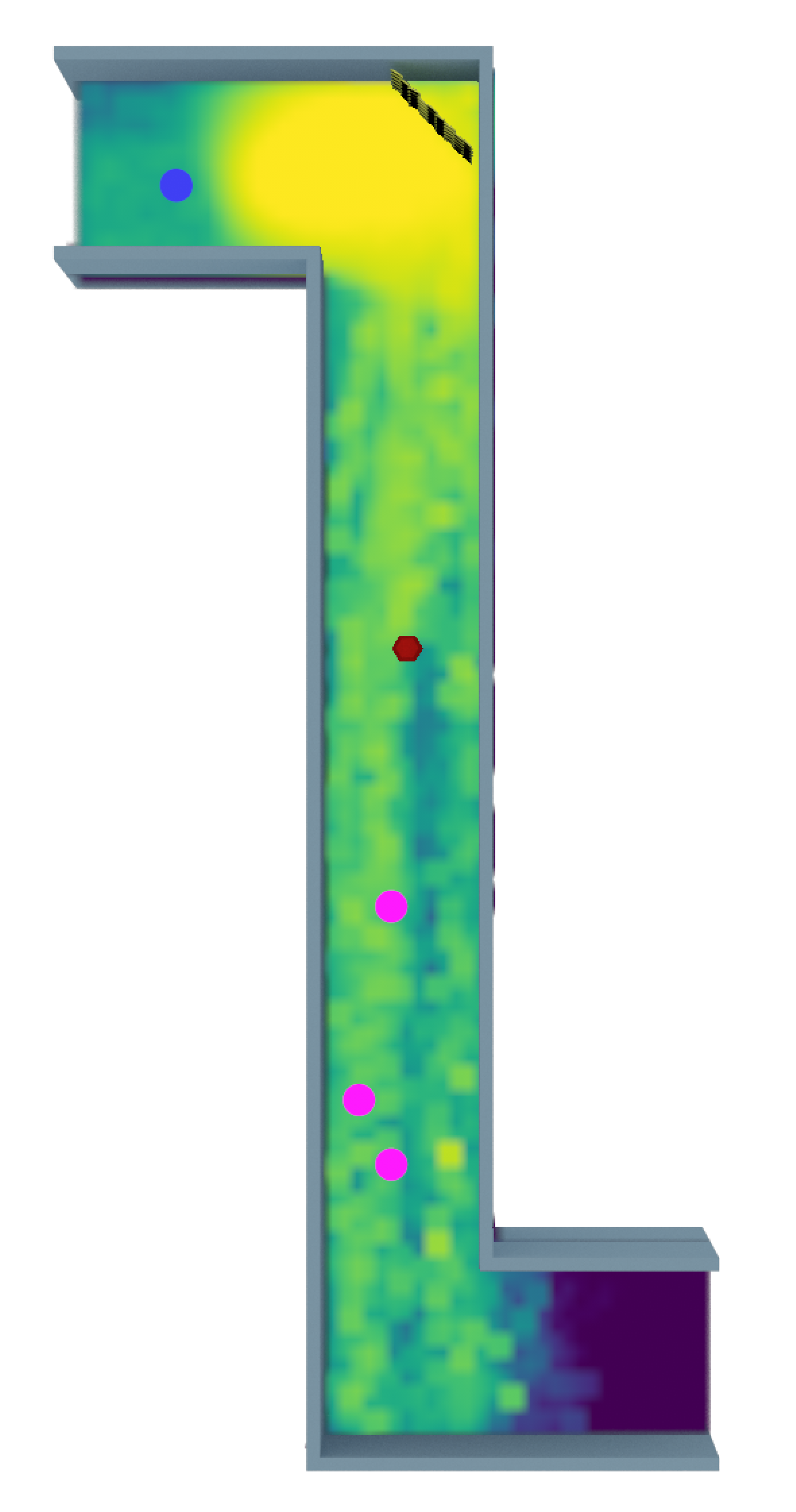
(d)

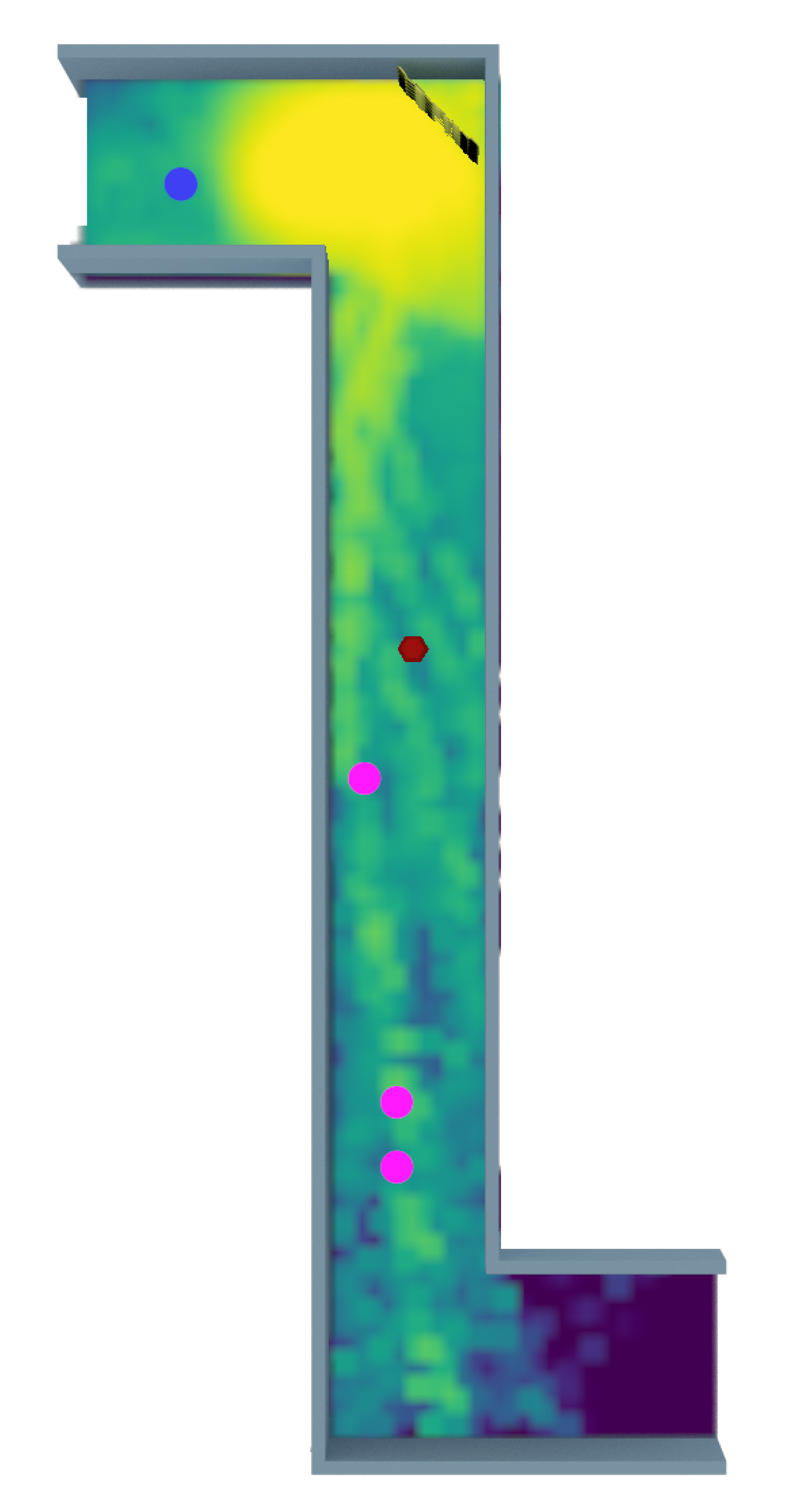
(e)

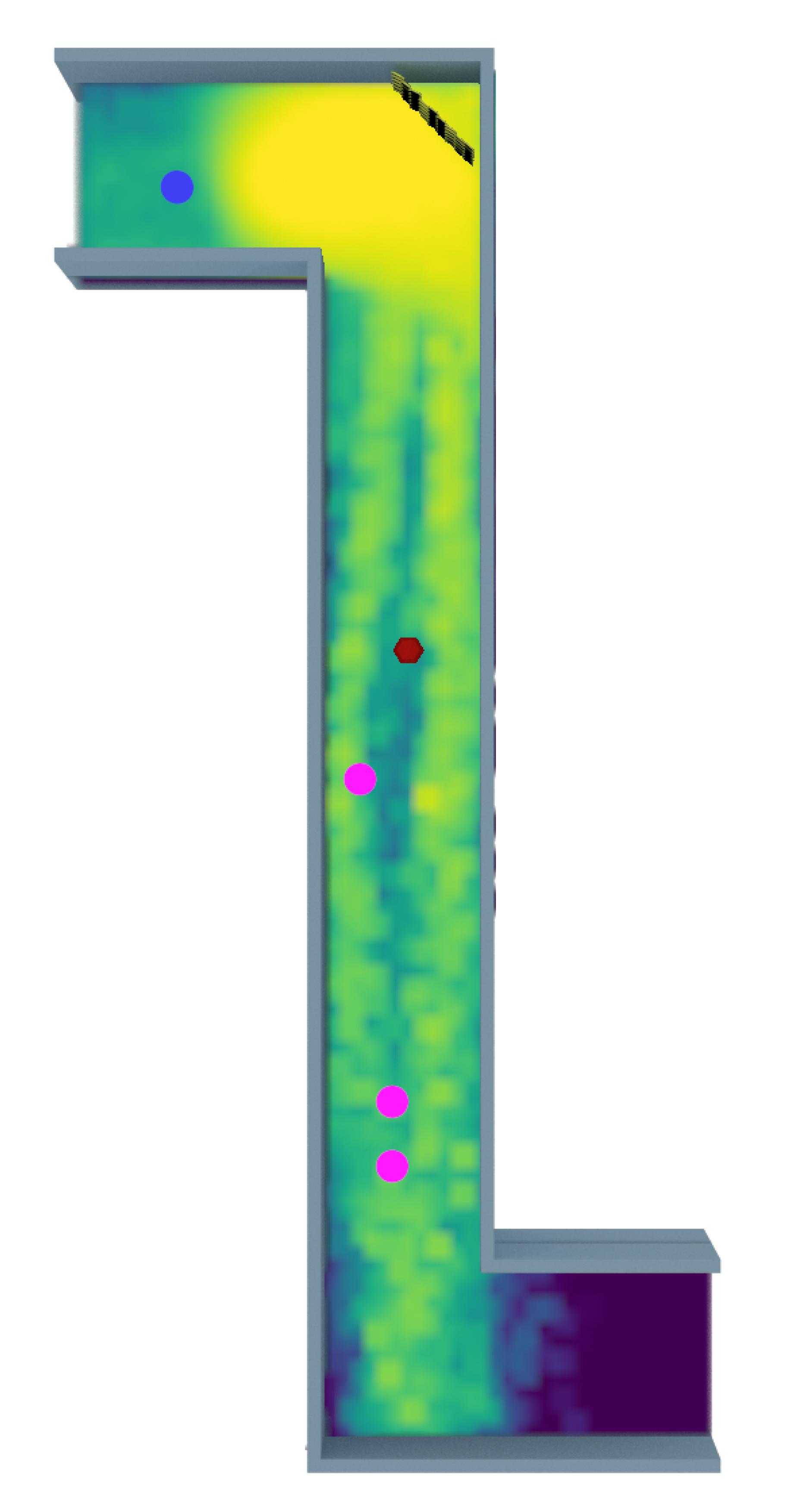
(f)

Figure 11: Evaluation results for randomized user position in an L-shaped hallway.

This scenario builds on the previous setup, with users randomly positioned along the hallway while the transmitter and reflector locations remain fixed. Experiments are conducted in an L-shaped hallway where user positions change periodically, with each episode lasting 70 steps. At the start of each episode, both user locations and reflector tile configurations are randomized.

Figure 9 illustrates the effectiveness of the DRL algorithm in adapting to varying user positions by learning the dynamics of the environment. It optimizes the configurations of the tiles to redirect signals, leading to a significant increase in episodic return, which correlates with the average path gain for all users. The observed fluctuations in reward are mainly attributed to the distances of users from the reflector; even when the reflector directs beams towards users located farther away, their path gain remains lower than when they are positioned closer. Consequently, despite the presence of several dips in episodic return shown in the figure, the agent is still able to improve the average path gain for all users over time.

The effectiveness of the DRL-based reflector is further evaluated through multiple evaluation experiments. Figure 10 illustrates the reflector’s capability to effectively redirect signals to all users across varying positions, resulting in an improvement of the average path gain from approximately $-84$ dB to $-75$ dB.

Figures 11(a) and 11(b) illustrate the autonomous configuration process of the reflector during evaluation. Within a few steps, the reflector effectively directs signal beams toward all users, even when their locations are randomized. The scale for all evaluation runs in this context is comparable to that presented in Figure 7. Likewise, Figures 11(c) through 11(f) demonstrate the adaptability of the DRL-based reflector. The system successfully reconfigures its tiles to redirect signals to the intended targets, maintaining performance despite changes in user positions and different initial tile configurations. This underscores the robustness and flexibility of the DRL-based approach in dynamic environments.

V-D Ablation Study for Network Size

To assess the impact of different design choices, we explored the influence of network capacity by varying the size of both the actor and critic networks, using configurations with 128 and 256 neurons in the fully connected layers and feed-forward blocks.

Figure 12: Comparison of episodic return during training for the scenario with fixed user positions with different size of neural network.

Figure 13: Comparison of episodic return during training for the scenario with randomized user positions with different size of neural network.

We begin by examining the effect of network size on the performance of the DRL algorithm in a fixed user position scenario. As shown in Figure 12, a 256-node network performs worse than a 128-node network. The larger network struggles to learn the environment’s dynamics, likely due to its increased complexity, which can lead to overfitting or inefficient learning when data is limited. Larger networks require more data to generalize effectively, and with insufficient training data, they may overfit or fail to converge, reducing adaptability. Smaller networks, like those with 128 nodes, are less prone to overfitting and generalize better [45].

This trend also persists in scenarios with randomized user positions, where the network with 128 neurons significantly outperforms the one with 256 neurons (Figure 13). Overall, these findings highlight that the size of the network is a critical hyperparameter affecting DRL performance.

VI Conclusion and Future Work

In conclusion, this research demonstrates the effectiveness of self-adjustable metallic surfaces guided by DRL in enhancing wireless signal reception. The proposed reflector array significantly outperformed baseline setups, achieving improvements in average path gain for multiple users under obstructed conditions. These findings contribute to the advancement of smart radio environments and provide a foundation for future practical applications that can dynamically adapt to real-world challenges. Future work will focus on refining the DRL algorithms and exploring additional scenarios, such as larger conference rooms with increased user density and more obstacles, to further enhance the adaptability and efficiency of wireless communication systems.

References

- [1] E. Björnson, H. Wymeersch, B. Matthiesen, P. Popovski, L. Sanguinetti, and E. De Carvalho, “Reconfigurable intelligent surfaces: A signal processing perspective with wireless applications,” IEEE Signal Processing Magazine, vol. 39, no. 2, pp. 135–158, 2022.
- [2] M. Di Renzo, A. Zappone, M. Debbah, M.-S. Alouini, C. Yuen, J. de Rosny, and S. Tretyakov, “Smart Radio Environments Empowered by Reconfigurable Intelligent Surfaces: How It Works, State of Research, and The Road Ahead,” IEEE Journal on Selected Areas in Communications, vol. 38, no. 11, pp. 2450–2525, 2020.
- [3] G. H.-h. Sung, K. W. Sowerby, M. J. Neve, and A. G. Williamson, “A frequency-selective wall for interference reduction in wireless indoor environments,” IEEE Antennas and Propagation Magazine, vol. 48, no. 5, pp. 29–37, 2006.
- [4] M. Raspopoulos and S. Stavrou, “Frequency selective buildings through frequency selective surfaces,” IEEE Transactions on Antennas and Propagation, vol. 59, no. 8, pp. 2998–3005, 2011.
- [5] R. S. Anwar, L. Mao, and H. Ning, “Frequency selective surfaces: A review,” Applied Sciences, vol. 8, no. 9, 2018. [Online]. Available: https://www.mdpi.com/2076-3417/8/9/1689
- [6] L. Subrt, D. Grace, and P. Pechac, “Controlling the Short-Range Propagation Environment Using Active Frequency Selective Surfaces,” RADIOENGINEERING, vol. 19, pp. 610–617, Dec. 2010.
- [7] J. Zhao, “A survey of intelligent reflecting surfaces (IRSs): Towards 6G wireless communication networks,” arXiv preprint arXiv:1907.04789, 2019.
- [8] S. Zahra, L. Ma, W. Wang, J. Li, D. Chen, Y. Liu, Y. Zhou, N. Li, Y. Huang, and G. Wen, “Electromagnetic Metasurfaces and Reconfigurable Metasurfaces: A Review,” Frontiers in Physics, vol. 8, 2021. [Online]. Available: https://www.frontiersin.org/articles/10.3389/fphy.2020.593411
- [9] S. Basharat, M. Khan, M. Iqbal, U. S. Hashmi, S. A. R. Zaidi, and I. Robertson, “Exploring reconfigurable intelligent surfaces for 6G: State-of-the-art and the road ahead,” IET Communications, vol. 16, no. 13, pp. 1458–1474, 2022. [Online]. Available: https://ietresearch.onlinelibrary.wiley.com/doi/abs/10.1049/cmu2.12364
- [10] C. Pan, G. Zhou, K. Zhi, S. Hong, T. Wu, Y. Pan, H. Ren, M. Di Renzo, A. L. Swindlehurst, R. Zhang et al., “An overview of signal processing techniques for RIS/IRS-aided wireless systems,” IEEE Journal of Selected Topics in Signal Processing, vol. 16, no. 5, pp. 883–917, 2022.
- [11] S. Kim, H. Lee, J. Cha, S.-J. Kim, J. Park, and J. Choi, “Practical channel estimation and phase shift design for intelligent reflecting surface empowered MIMO systems,” IEEE Transactions on Wireless Communications, vol. 21, no. 8, pp. 6226–6241, 2022.
- [12] Q. Wu and R. Zhang, “Intelligent reflecting surface enhanced wireless network via joint active and passive beamforming,” IEEE transactions on wireless communications, vol. 18, no. 11, pp. 5394–5409, 2019.
- [13] H. Yang, X. Cao, F. Yang, J. Gao, S. Xu, M. Li, X. Chen, Y. Zhao, Y. Zheng, and S. Li, “A programmable metasurface with dynamic polarization, scattering and focusing control,” Scientific reports, vol. 6, no. 1, pp. 1–11, 2016.
- [14] W. Tang, X. Li, J. Y. Dai, S. Jin, Y. Zeng, Q. Cheng, and T. J. Cui, “Wireless communications with programmable metasurface: Transceiver design and experimental results,” China Communications, vol. 16, no. 5, pp. 46–61, 2019.
- [15] H. Jeong, E. Park, R. Phon, and S. Lim, “Mechatronic reconfigurable intelligent-surface-driven indoor fifth-generation wireless communication,” Advanced Intelligent Systems, vol. 4, no. 12, p. 2200185, 2022. [Online]. Available: https://onlinelibrary.wiley.com/doi/abs/10.1002/aisy.202200185
- [16] H. Le, O. Bedir, M. Ibrahim, J. Tao, and S. Ekin, “Guiding Wireless Signals with Arrays of Metallic Linear Fresnel Reflectors: A Low-cost, Frequency-versatile, and Practical Approach,” arXiv preprint arXiv:2407.19179, 2024.
- [17] Qualcomm. (2024) Unlocking on-device generative AI with an NPU and heterogeneous computing. [Online]. Available: https://www.qualcomm.com/content/dam/qcomm-martech/dm-assets/documents/Unlocking-on-device-generative-AI-with-an-NPU-and-heterogeneous-computing.pdf
- [18] A. Nasari, H. Le, R. Lawrence, Z. He, X. Yang, M. Krell, A. Tsyplikhin, M. Tatineni, T. Cockerill, L. Perez, D. Chakravorty, and H. Liu, “Benchmarking the performance of accelerators on national cyberinfrastructure resources for artificial intelligence / machine learning workloads,” in Practice and Experience in Advanced Research Computing 2022: Revolutionary: Computing, Connections, You, ser. PEARC ’22. New York, NY, USA: Association for Computing Machinery, 2022. [Online]. Available: https://doi.org/10.1145/3491418.3530772
- [19] H. Le, Z. He, M. Le, D. Chakravorty, L. M. Perez, A. Chilumuru, Y. Yao, and J. Chen, “Insight Gained from Migrating a Machine Learning Model to Intelligence Processing Units,” in Practice and Experience in Advanced Research Computing 2024: Human Powered Computing, ser. PEARC ’24. New York, NY, USA: Association for Computing Machinery, 2024. [Online]. Available: https://doi.org/10.1145/3626203.3670527
- [20] C. Silvano, D. Ielmini, F. Ferrandi, L. Fiorin, S. Curzel, L. Benini, F. Conti, A. Garofalo, C. Zambelli, E. Calore et al., “A survey on deep learning hardware accelerators for heterogeneous hpc platforms,” arXiv preprint arXiv:2306.15552, 2023.
- [21] C. Huang, R. Mo, and C. Yuen, “Reconfigurable intelligent surface assisted multiuser MISO systems exploiting deep reinforcement learning,” IEEE Journal on Selected Areas in Communications, vol. 38, no. 8, pp. 1839–1850, 2020.
- [22] A. Taha, Y. Zhang, F. B. Mismar, and A. Alkhateeb, “Deep reinforcement learning for intelligent reflecting surfaces: Towards standalone operation,” in 2020 IEEE 21st international workshop on signal processing advances in wireless communications (SPAWC). IEEE, 2020, pp. 1–5.
- [23] A. Taha, M. Alrabeiah, and A. Alkhateeb, “Enabling large intelligent surfaces with compressive sensing and deep learning,” IEEE access, vol. 9, pp. 44 304–44 321, 2021.
- [24] B. Sheen, J. Yang, X. Feng, and M. M. U. Chowdhury, “A deep learning based modeling of reconfigurable intelligent surface assisted wireless communications for phase shift configuration,” IEEE Open Journal of the Communications Society, vol. 2, pp. 262–272, 2021.
- [25] H. Choi, L. V. Nguyen, J. Choi, and A. L. Swindlehurst, “A Deep Reinforcement Learning Approach for Autonomous Reconfigurable Intelligent Surfaces,” arXiv preprint arXiv:2403.09270, 2024.
- [26] W. Wang and W. Zhang, “Intelligent reflecting surface configurations for smart radio using deep reinforcement learning,” IEEE Journal on Selected Areas in Communications, vol. 40, no. 8, pp. 2335–2346, 2022.
- [27] X. He and W. Jia, “Hexagonal structure for intelligent vision,” in 2005 International Conference on Information and Communication Technologies. IEEE, 2005, pp. 52–64.
- [28] I. T. U. R. Sector. (2024) Effects of building materials and structures on radiowave propagation above about 100MHz. [Online]. Available: https://www.itu.int/rec/R-REC-P.2040/en
- [29] J. B. Keller, “Geometrical theory of diffraction,” Josa, vol. 52, no. 2, pp. 116–130, 1962.
- [30] R. G. Kouyoumjian and P. H. Pathak, “A uniform geometrical theory of diffraction for an edge in a perfectly conducting surface,” Proceedings of the IEEE, vol. 62, no. 11, pp. 1448–1461, 1974.
- [31] D. Porcino and W. Hirt, “Ultra-wideband radio technology: potential and challenges ahead,” IEEE communications magazine, vol. 41, no. 7, pp. 66–74, 2003.
- [32] J. Hoydis, S. Cammerer, F. Ait Aoudia, A. Vem, N. Binder, G. Marcus, and A. Keller, “Sionna: An Open-Source Library for Next-Generation Physical Layer Research,” arXiv preprint, Mar. 2022.
- [33] Blender. (2024) The Blender Foundation. [Online]. Available: https://www.blender.org/
- [34] C. A. Balanis, Advanced engineering electromagnetics. John Wiley & Sons, 2012.
- [35] N. Geng and W. Wiesbeck, Planungsmethoden für die Mobilkommunikation: Funknetzplanung unter realen physikalischen Ausbreitungsbedingungen. Springer-Verlag, 2013.
- [36] T. Haarnoja, A. Zhou, P. Abbeel, and S. Levine, “Soft actor-critic: Off-policy maximum entropy deep reinforcement learning with a stochastic actor,” in International conference on machine learning. PMLR, 2018, pp. 1861–1870.
- [37] T. Haarnoja, A. Zhou, K. Hartikainen, G. Tucker, S. Ha, J. Tan, V. Kumar, H. Zhu, A. Gupta, P. Abbeel et al., “Soft actor-critic algorithms and applications,” arXiv preprint arXiv:1812.05905, 2018.
- [38] T. Lillicrap, “Continuous control with deep reinforcement learning,” arXiv preprint arXiv:1509.02971, 2015.
- [39] S. Fujimoto, H. Hoof, and D. Meger, “Addressing function approximation error in actor-critic methods,” in International conference on machine learning. PMLR, 2018, pp. 1587–1596.
- [40] J. Schulman, F. Wolski, P. Dhariwal, A. Radford, and O. Klimov, “Proximal policy optimization algorithms,” arXiv preprint arXiv:1707.06347, 2017.
- [41] B. Mildenhall, P. P. Srinivasan, M. Tancik, J. T. Barron, R. Ramamoorthi, and R. Ng, “Nerf: Representing scenes as neural radiance fields for view synthesis,” Communications of the ACM, vol. 65, no. 1, pp. 99–106, 2021.
- [42] M. Tancik, P. Srinivasan, B. Mildenhall, S. Fridovich-Keil, N. Raghavan, U. Singhal, R. Ramamoorthi, J. Barron, and R. Ng, “Fourier features let networks learn high frequency functions in low dimensional domains,” Advances in neural information processing systems, vol. 33, pp. 7537–7547, 2020.
- [43] A. Vaswani, “Attention is all you need,” Advances in Neural Information Processing Systems, 2017.
- [44] H. Le. (2025) DRL-controlled Reflector Videos for an L-shaped Hallway. [Online]. Available: https://youtube.com/playlist?list=PLqlwvIIAd0I7tu3LIuCx8X7pMU0s1mXtV&si=H8AkazyF4dPoQ3iF
- [45] K. Ota, D. K. Jha, and A. Kanezaki, “A framework for training larger networks for deep reinforcement learning,” Machine Learning, pp. 1–25, 2024.