Divergence-Augmented Policy Optimization

Qing Wang, Yingru Li, Jiechao Xiong, Tong Zhang

\setbeamercolor

block titlefg=ngreen,bg=white \setbeamercolorblock bodyfg=black,bg=white \setbeamercolorblock alerted titlefg=white,bg=dblue!70 \setbeamercolorblock alerted bodyfg=black,bg=dblue!10 \setbeamertemplatebibliography entry location \instituteHuya AI, CUHK-Shenzhen, Tencent AI Lab, HKUST

\addtobeamertemplate

block end \addtobeamertemplateblock alerted end

{columns}

[t]

{column}

\setbeamercolor

block alerted titlefg=white,bg=RubineRed \setbeamercolorblock alerted bodyfg=black,bg=white {alertblock}Overview We study the divergence augmented policy optimization method in which the optimization is guided by divergence augmented reward $r_{i}-1/\eta\log\frac{\pi_{\theta}}{\pi_{\theta_{t}}}$ instead of original $r_{i}$ .

The method is to introduce divergence regularization to stabilize policy optimization when off-policy data are reused. We show that the above formation of divergence augmentation can be derived from the Bregman divergence calculated between the state-action distributions of two policies, instead of only on the action probabilities.

Empirical experiments on Atari games show that in the data-scarce scenario where the reuse of off-policy data becomes necessary, our method can achieve better performance than other state-of-the-art deep reinforcement learning algorithms.

{block}

Preliminaries We define the Bregman divergence as follows: With respect to a Legendre $F$ , we define the Bregman divergence $D_{F}:\bar{\mathcal{D}}\times\mathcal{D}\rightarrow\mathbb{R}$ as

D_{F}(x,y)=F(x)-F(y)-\langle\nabla F(y),x-y\rangle.

The inner product is defined as $\langle x,y\rangle=\Sigma_{i}x_{i}y_{i}$ . For $\mathcal{K}\subset\bar{\mathcal{D}}$ and $\mathcal{K}\cap\mathcal{D}\neq\emptyset$ , the Bregman projection

z=\operatorname*{arg\,min}_{x\in\mathcal{K}}D_{F}(x,y)

exists uniquely for all $y\in\mathcal{D}$ . Specifically, for $F(x)=\Sigma_{i}x_{i}\log(x_{i})-\Sigma_{i}x_{i}$ , we recover the Kullback-Leibler (KL) divergence as

\displaystyle D_{\text{KL}}(\mu^{\prime},\mu)

\displaystyle=

\displaystyle\Sigma_{s,a}\mu^{\prime}(s,a)\log\frac{\mu^{\prime}(s,a)}{\mu(s,a)}

for $\mu,\mu^{\prime}\in\Delta(\mathcal{S}\times\mathcal{A})$ and $\pi,\pi^{\prime}\in\Pi$ . To measure the distance between two policies $\pi$ and $\pi^{\prime}$ , we also use the symbol for conditional “Bregman divergence” associated with state distribution $d$ denoted as

\displaystyle D_{F}^{d}(\pi^{\prime},\pi)=\Sigma_{s}d(s)D_{F}(\pi^{\prime}(\cdot|s),\pi(\cdot|s)).

(1)

{column}

\setbeamercolor

block alerted titlefg=white,bg=ProcessBlue \setbeamercolorblock alerted bodyfg=black,bg=white {alertblock}Motivation Given the policy at iteration $t$ as

\mu_{t}(s,a)=d_{t}(s)\pi_{t}(a|s)

we would like to find a $\mu_{t+1}$ which is close to $\mu_{t}$ . Inspired from mirror descent methods, given the gradient of loss as $g_{t}$ and $\tilde{\mu}_{t+1}\propto\mu_{t}\exp(-\eta g_{t})$ , it is known that

	$\displaystyle\mu_{t+1}$	$\displaystyle=$	$\displaystyle\operatorname*{arg\,min}_{\mu\in\Delta_{\Pi}}D_{\text{KL}}(\mu,\tilde{\mu}_{t+1}),$		(2)
	$\displaystyle\mu_{t+1}$	$\displaystyle=$	$\displaystyle\operatorname*{arg\,min}_{\mu\in\Delta_{\Pi}}D_{\text{KL}}(\mu,\mu_{t})+\eta\langle g_{t},\mu\rangle$		(3)

are equivalent. In addition, if we reverse the KL divergence in (2), we get

\mu_{t+1}=\operatorname*{arg\,min}_{\mu\in\Delta_{\Pi}}D_{\text{KL}}(\tilde{\mu}_{t+1},\mu)

which recovers the core algorithm as in MPO and MARWIL; while if we reverse the KL divergence in (3), we get

\mu_{t+1}=\operatorname*{arg\,min}_{\mu\in\Delta_{\Pi}}D_{\text{KL}}(\mu_{t},\mu)+\eta\langle g_{t},\mu\rangle,

which is related to the TRPO method. Although TRPO and MPO have been widely used in reinforcement learning community, the original formulation in (2) (3) is more natural in this view.

\setbeamercolor

block alerted titlefg=white,bg=VioletRed \setbeamercolorblock alerted bodyfg=black,bg=white {alertblock}Divergence-Augmented Policy Optimization (DAPO) Input: $D_{F}(\mu^{\prime},\mu)$ , total iteration $T$ , batch size $M$ , learning rate $\alpha_{t}$ .
Initialize : randomly initiate $\theta_{0}$
— For $t=0$ to $T$
— (in parallel) Use $\pi_{t}=\pi_{\theta_{t}}$ to generate trajectories.
— For $m=1$ to $M$
— Sample $(s_{i},a_{i})\in\mathcal{S}\times\mathcal{A}$ w.p. $d_{t}\pi_{t}$ .
— Estimate state value $v_{s_{i}}$ (e.g. by V-trace).
— Calculate Q-value est. $\hat{A}_{s,a}$ and divergence est. $\hat{D}_{s,a}$ .
— $\quad\hat{A}_{s,a}=r_{i}+\gamma v_{i+1}-V_{\theta}(s_{i})$ ,
— $\quad\hat{D}_{s,a}=f(s_{i},a_{i})+\Sigma_{j=1}^{n}\gamma^{j}(\Pi_{k=0}^{j-1}c_{i+k})\rho_{i+j}f(s_{i+j},a_{i+j})$ .
— Update $\theta$ with respect of policy loss and value loss
— $\quad\theta\leftarrow\theta-\alpha_{t}(\nabla_{\theta}L_{\pi}(\theta)+{b}\nabla_{\theta}L_{v}(\theta)).$
— Set $\theta_{t+1}=\theta$ .

{column}

{column}\setbeamercolor

block alerted titlefg=white,bg=Green \setbeamercolorblock alerted bodyfg=black,bg=white {alertblock}Divergence Augmentation Solving (3) is usually hard. We consider the optimization of (3) in the (parametric) policy space without explicit projection to $\Delta_{\Pi}$ . Specifically, we consider $\mu_{\pi}$ as a function of $\pi$ , and $\pi$ parametrized as $\pi_{\theta}$ . The Formula (3) can be written as

\displaystyle\pi_{t+1}=\operatorname*{arg\,min}_{\pi}D_{F}(\mu_{\pi},\mu_{t})+\eta\langle g_{t},\mu_{\pi}\rangle.

(4)

Instead of solving globally, we approximate Formula (4) with gradient descent on $\pi$ . From the celebrated policy gradient theorem, we have

\Sigma_{s,a}f(s,a)\nabla_{\theta}\mu_{\pi}(s,a)=\Sigma_{s,a}d_{\pi}(s)\mathcal{Q}^{\pi}(f)(s,a)\nabla_{\theta}\pi(a|s),

for any state-action function $f:\mathcal{S}\times\mathcal{A}\rightarrow\mathbb{R}$ , and $\mathcal{Q}^{\pi}(\cdot)$ defined as an operator such that

\displaystyle\mathcal{Q}^{\pi}(f)(s,a)={\mathbb{E}}_{\pi|s_{t}=s,a_{t}=a}\Sigma_{l=0}^{\infty}\gamma^{l}f(s_{t+l},a_{t+l}).

Decomposing the loss and divergence in two parts (4), we have

\displaystyle\nabla_{\theta}\left\langle g_{t},\mu_{\pi}\right\rangle=\left\langle d_{\pi}\mathcal{Q}^{\pi}(g_{t}),\nabla_{\theta}\pi(a|s)\right\rangle,

(5)

which is the usual policy gradient, and

\displaystyle\nabla_{\theta}D_{F}(\mu_{\pi},\mu_{t})=\left\langle d_{\pi}\mathcal{Q}^{\pi}\left(\nabla F(\mu_{\pi})-\nabla F(\mu_{t})\right),\nabla_{\theta}\pi(a|s)\right\rangle.

(6)

We utilize the V-trace estimation of $\mathcal{Q}^{\pi}(g_{t})$ and $\mathcal{Q}^{\pi}(\nabla F(\mu_{\pi})-\nabla F(\mu_{t}))$ as $\hat{A}_{s,a}$ and $\hat{D}_{s,a}$ . The gradient of policy loss is

\displaystyle\nabla_{\theta}L_{\pi}(\theta)={\mathbb{E}}_{\pi_{t},d_{t}}\frac{\pi}{\pi_{t}}(\hat{D}_{s,a}-\eta\hat{A}_{s,a})\nabla_{\theta}\log\pi.

(7)

which explains the name “divergence augmentation”.

\setbeamercolor

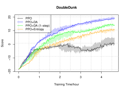
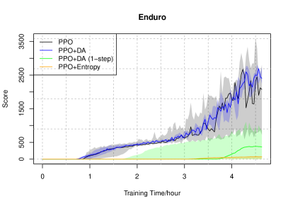
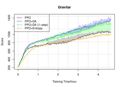
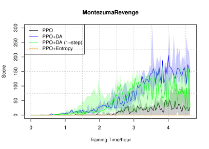
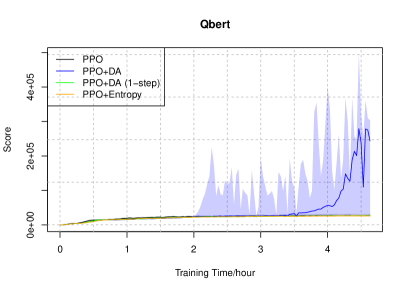
block alerted titlefg=white,bg=Purple \setbeamercolorblock alerted bodyfg=black,bg=white {alertblock}Performance Comparison [Uncaptioned image] PPO with and without Divergence Augmentation. We see relatively better performance in data-scarce scenarios.

{column}

{column}

{block}

Experiments

Refer to caption — Figure 1: Performance comparison on selected environments of Atari games. The performance of PPO, PPO+DA, PPO+DA (1-step), and PPO+Entropy are plotted in different colors.

\usebeamerfont

block body

\setbeamercolor

block alerted titlefg=white,bg=YellowGreen \setbeamercolorblock alerted bodyfg=black,bg=white {alertblock}Conclusion In short, we showed that divergence augmentation can be viewed as imposing Bregman divergence constraint on the state-action space, which is related to online mirror descent methods. Experiments results showed that divergence augmentation is effective when data generated by previous policies are reused in policy optimization.