lemmatheorem \aliascntresetthelemma \newaliascntpropositiontheorem \aliascntresettheproposition \newaliascntcorollarytheorem \aliascntresetthecorollary \newaliascntconjecturetheorem \aliascntresettheconjecture \newaliascntopenQtheorem \aliascntresettheopenQ \newaliascntquesttheorem \aliascntresetthequest \newaliascntquestxconjx \aliascntresetthequestx \newaliascntdefntheorem \aliascntresetthedefn \newaliascntexampletheorem \aliascntresettheexample \newaliascntremtheorem \aliascntresettherem
Two disks maximize the third Robin eigenvalue: positive parameters
Abstract.
The third eigenvalue of the Robin Laplacian on a simply-connected planar domain of given area is bounded above by the corresponding eigenvalue of a disjoint union of two equal disks, for Robin parameters in . This sharp inequality was known previously only for negative parameters in , by Girouard and Laugesen. Their proof fails for positive Robin parameters because the second eigenfunction on a disk has non-monotonic radial part. This difficulty is overcome for parameters in by means of a degree-theoretic approach suggested by Karpukhin and Stern that yields suitably orthogonal trial functions.
Key words and phrases:
Robin, Neumann, vibrating membrane, conformal mapping2010 Mathematics Subject Classification:
Primary 35P15. Secondary 30C701. Introduction
The Robin eigenvalue problem for a bounded Lipschitz planar domain consists of finding eigenvalues of the Laplacian for which an eigenfunction exists satisfying
where is the outward normal derivative, is the length (perimeter) of the boundary , and is the Robin parameter. We choose in the boundary condition to divide by in order to match the inverse length scale of the normal derivative . Consequently, the parameter below in Theorem 1.1 belongs to a universal interval that is independent of the shape of and of its area .
Physically, Robin eigenvalues represent rates of decay to equilibrium for heat in a partially insulated region, or frequencies of vibration for a membrane under elastically restoring boundary conditions.
Sharp upper bounds are known for the first three Robin eigenvalues. After multiplying the eigenvalue by the area to obtain a scale invariant quantity, is known to be maximal for a degenerate rectangle, for each ; see [3, Theorem A]. The second eigenvalue is maximal among simply-connected domains for the disk whenever , as shown by Freitas and Laugesen [3, Theorem B]. While this interval of -values could perhaps be enlarged, the disk certainly cannot be the maximizer for all , because the Robin spectrum converges to the Dirichlet spectrum as and the lowest Dirichlet eigenvalue can be made arbitrarily large by considering thin domains of fixed area.
For the third Robin eigenvalue, Girouard and Laugesen [5, Theorem 1.1] proved a sharp upper bound when lies in the interval : they proved is maximized by a disjoint union of two equal disks, in the sense that this maximum value is approached in the limit as a simply-connected domain degenerates to a union of disks.
The goal of this paper is to extend Girouard and Laugesen’s upper bound to handle positive Robin parameters in the range , thus resolving one of their open problems [5, p. 2713]. Write for the unit disk, so that represents a disjoint union of two copies of the disk.
Theorem 1.1 (Third Robin eigenvalue is maximal for two disks).
Fix . If is a simply-connected bounded Lipschitz domain whose boundary is a Jordan curve then
Equality is attained asymptotically for the domain that as approaches the disjoint union of two disks.
The third eigenvalue of the disjoint union is simply the second eigenvalue of one of the disks, and so the theorem says
where the eigenvalue on the right can be computed explicitly in terms of Bessel functions on the disk, as explained in Appendix A.
By scale invariance, the conclusion of the theorem can alternatively be rephrased as
where is the union of two disjoint disks each having half the area of .
As a remark, Theorem 1.1 can fail when , because by [3, pp. 1039–1040] when , while by [3, (4.1)] we have for any sufficiently long and thin rectangle .
Plan of the paper
The next section explains how to modify Girouard and Laugesen’s approach in order to obtain Theorem 1.1 for . The key change is to use a degree theoretic lemma due to Karpukhin and Stern [9, Lemma 4.2] for mappings between spheres. Those authors wrote in reference to the theorem of Girouard and Laugesen for that “We believe that our version of the argument allows one to extend the range of Robin parameters for which the results” hold [9, p. 4079]. The current paper pursues their suggestion and shows that the crucial reflection-symmetry hypothesis ((6)) indeed holds, enabling the proof to proceed.
Section 3 recalls properties of Möbius transformations and hyperbolic caps. From those objects the family of trial functions is constructed: see formula ((2)) and Figure 2.
To show in Section 4 that at least one trial function in the family is orthogonal to the first two Robin eigenfunctions of , the reflection symmetry hypothesis for Karpukhin and Stern’s degree theory lemma is verified. In Section 5 we present an alternative proof of Kim’s variant of their lemma [11]. We simplify Kim’s proof by introducing a homotopy to avoid certain calculations, thus bringing out more clearly the role played by the reflections.
Appendix A collects background facts on the Robin spectrum of the disk.
Literature on upper bounds for eigenvalues of the Laplacian
The maximization of individual eigenvalues of the Laplacian began with Szegő [14], who proved that among simply-connected planar domains of given area, the second Neumann () eigenvalue is largest for the disk. Weinberger [15] extended the result by a different method to domains in all dimensions. An excellent source for these classical results and later developments is the survey book edited by Henrot [7]. Notable open problems for Robin eigenvalues can also be found in Laugesen [12].
The Neumann inequalities of Szegő and Weinberger were extended to the second Robin eigenvalue by Freitas and Laugesen [3, 4]. For the third Neumann eigenvalue, the breakthrough was achieved by Girouard, Nadirashvili and Polterovich [6], finding for simply connected planar domains that the maximizer is the union of two equal disks. Their result was generalized by Bucur and Henrot [1] to all domains and higher dimensions.
Meanwhile, a parallel line of research developed eigenvalue bounds on closed surfaces and manifolds, starting with Hersch’s generalization of Szegő’s approach to metrics on the -sphere [8], showing that the round sphere maximizes . The most relevant work for our current purposes is by Petrides [13], Karpukhin and Stern [9] and Kim [10, 11]. Petrides got upper bounds on for spheres of arbitrary dimensions, and in the course of that work obtained an elegant degree theory lemma for “reflection symmetric” maps between spheres [13, claim 3].
Karpukhin and Stern found a more general result [9, Lemma 4.2] involving two reflections rather than one. Kim applied Petrides’s lemma in her work for eigenvalues on spheres [10] and applied a variant of Karpukhin and Stern’s lemma to eigenvalues on projective space [11]. In the latter paper, she provided an alternative proof that yields more information about the value of the degree of the sphere mapping.
2. Proof of Theorem 1.1
The function spaces and consist of complex-valued functions, although for the sake of brevity we will often omit the from the notation. A conformal map is a diffeomorphism that is holomorphic in both directions.
The Robin eigenvalues form a sequence in which each eigenvalue is repeated according to its multiplicity. The variational characterization of the third eigenvalue says that it equals the minimum of the Rayleigh quotient taken over trial functions orthogonal to the first two eigenfunctions:
where and are -orthonormal real-valued eigenfunctions corresponding to the eigenvalues and , and is the area element. The trial function may be complex-valued.
Thus to prove Theorem 1.1, one wants to construct a suitable trial function and show that when it is substituted into the variational characterization, the desired upper bound is obtained on the third eigenvalue.
The method of Girouard and Laugesen [5, Section 7] for continues to hold verbatim for , except with one minor and one major alteration. The major change is that when , a new method is needed to prove existence of a trial function orthogonal to the Robin eigenfunctions and . Girouard and Laugesen take a two-step approach to proving orthogonality. In terms of the notation developed in Section 3 below, their first step shows for each each hyperbolic cap that a unique Möbius parameter exists that ensures orthogonality of against (their Lemma 5.1 and (5.3)). Second, they show for some that orthogonality also holds against (their Proposition 5.5). The hypothesis of their first step fails when because the second Robin eigenfunction of a disk has nonmonotonic radial part ; see Figure 5 in Appendix A.
To replace the orthogonality component of their argument, in the current paper we rely on Section 4 below to generate a trial function that is orthogonal to and . The proof of that proposition follows the one-step approach of Karpukhin and Stern.
The proposition generates a trial function that depends on a point and a parameter . When , Case 2 in the proof of Girouard and Laugesen [5, Sections 7] should be followed. When , one follows Case 1 with the minor change that in their proof is replaced by .
The final claim in the theorem, about asymptotic equality as , was handled for all by Girouard and Laugesen [5, Section 8]. ∎
Remark
The orthogonality construction in Section 4 holds for all . The restriction in Theorem 1.1 is necessary elsewhere in the proof of the theorem, on [5, pp. 2732-2733], to ensure nonnegativity of and hence to justify a certain inequality in the proof. The restriction arises on [5, pp. 2732–2733] when Girouard and Laugesen use their Lemmas 4.3 and 6.1 to compare the norm of the trial function on with the norm of the eigenfunction on . Those lemmas, which ultimately rely on [3, formula (7.5)], both require .
3. Möbius transformations, hyperbolic caps, fold and cap maps, and trial functions
We follow Girouard and Laugesen’s construction in [5] of a -parameter family of complex-valued trial functions for the Rayleigh quotient of . The four parameters will provide enough degrees of freedom to ensure at least one of the trial functions is orthogonal to the first two real-valued eigenfunctions and .
Two of the four parameters come from a family of Möbius transformations of the disk and two more from a family of hyperbolic caps inside the disk. We proceed to recall the needed formulas and reflection properties.
Möbius transformations
Given , let
When , this is a Möbius self-map of the disk with . When it is a constant map, with for all .
Define to be reflection across the line through the origin that is perpendicular to . The following conjugation relation comes from [5, formula (2.4)]:
| ((1)) |
Hyperbolic caps
For , let be the half-disk “centered” in direction :
where in this definition we think of and as vectors in . Define a hyperbolic cap by
as illustrated in Figure 1. The complement of is the cap .
The hyperbolic reflection associated with is obtained by pulling back to the half-disk, reflecting, and then pushing out again:
This reflection takes to and vice versa.
This paper uses only the caps with , that is, caps larger than a half-disk. It will be important later that expands to the full disk as .
Fold map
Define the “fold map” by
We interpret as “folding” the disk onto the cap across the boundary between and its complement . The fold map is two-to-one except on the common boundary. Clearly depends continuously on the parameters .
Cap map
Girouard and Laugesen [5, Section 3] constructed a particular conformal map , called a “cap map”, such that converges locally uniformly to the identity as , that is, as the cap expands to fill the whole disk.
Trial functions
Let . For the rest of the paper,
is the complex-valued Robin eigenfunction on the unit disk corresponding to ; see Appendix A, where it is observed that . The Robin parameter here is .
Fix a conformal map . Given a hyperbolic cap and , define the trial function
by
| ((2)) |
as shown schematically in Figure 2. This function is continuous as a function of , is bounded by the maximum value of the radial part , is smooth except along the preimage under of the cap boundary, and belongs to by conformal invariance of the Dirichlet integral.
Further, the trial function depends continuously on its parameters:
Lemma \thelemma (Continuous dependence of trial function; [5, Lemma 5.2]).
The function depends continuously on , in other words, on .
As the cap expands to the whole disk, the fold and cap maps drop out of the formula completely, yielding a limiting value at that is independent of the cap direction :
Lemma \thelemma (Extension of trial function to large caps; [5, Lemma 5.3]).
The function with extends to as follows:
with locally uniform convergence on .
4. Orthogonality of trial functions
Denote by and the first and second eigenfunctions (real-valued) of the Robin Laplacian on , corresponding to eigenvalues and , where . As explained in Section 2, the task for proving Theorem 1.1 is to show that for some and Möbius parameter , the trial function constructed in the previous section is -orthogonal to and . In Section 4 below, we establish the desired orthogonality.
Since the ground state does not change sign, we may suppose it is positive. Define
so that . Introduce a continuous vector field
that is defined by
The vector field extends continuously to with value
| ((3)) |
by Section 3 and dominated convergence, using that is dominated by the maximum value of . Notice this value in ((3)) is independent of and depends only on .
Another useful property is that when the value of is nonzero and independent of and , with
| ((4)) |
since for all while with , and and .
The goal is to show the vector field vanishes at some , because implies that is orthogonal in to and and hence also to . The next proposition uses homotopy invariance of degree to show that indeed vanishes somewhere.
Proposition \theproposition (Vanishing of the vector field).
for some and .
The provided by the proposition cannot lie in , due to ((4)), and so .
Proof.
We start by endowing an equivalence relation on the parameter space: say that if and . Then define a bijection to the -sphere by
where it is straightforward to check that . This mapping collapses the boundary points onto points in of the form . The inverse map has
when , where really depends only on since . When , we have and so , giving with an arbitrary point in (they are all equivalent under ).
Next, write the components of the inverse map as
| ((5)) |
Precompose the vector field with this inverse, letting
and noting when that the choice of is irrelevant because then , in which case is independent of by ((4)). Thus is continuous on .
Suppose for the sake of obtaining a contradiction that does not vanish. Then also does not vanish. Normalize by defining
with
Formula ((4)) implies when that .
We claim has degree . Indeed, when we have
by ((3)), and this last expression is independent of . Hence the continuous map is not surjective, because it depends only on the -dimensional parameter , is constant when , and is smooth when . Since the range of omits some point of , we see is homotopic to a constant map and so has degree . Homotopy invariance of degree implies that also has degree .
We will apply Theorem 5.1 below to to obtain the desired contradiction, namely that has degree . Hence we need only verify that satisfies the “reflection symmetry” hypothesis (7) in Theorem 5.1. In this task some shorthand notations are helpful, for the reflection, cap map and fold map associated with the half-disk: let and . Then for and , the definitions say that
using by ((5)) and linearity of , and that by [5, formula (5.5)] and by definition of the fold map. Since also by ((1)) and by [5, formula (5.6)], we deduce
| ((6)) |
The reflection preserves the magnitude, and so . Thus after dividing by these quantities, we see , which is the reflection symmetry condition (7) for .
Hence has degree by Theorem 5.1. This contradiction implies that must vanish somewhere, completing the proof of Section 4. ∎
5. Degree theory result
This section states and proves Theorem 5.1, which was used in the previous section and says that reflection-symmetric self-maps of have degree .
The degree of a continuous mapping from a sphere to itself is defined to equal , that is, the degree of at with respect to where is any continuous extension of to the ball ; see [2, Proposition 1.27].
Recall that is reflection across the line through the origin that is perpendicular to . Define
by when .
Theorem 5.1 (Degree of reflection-symmetric map between -spheres).
Suppose is continuous. If satisfies the reflection symmetry property
| ((7)) |
for all with , then .
The reflection symmetry condition ((7)) can be interpreted as saying that commutes with , since . But one must remember that the reflection operator depends on and so varies from point to point.
A recent paper by Kim [11, Theorem 11] shows that the degree of a map with reflection symmetry on equals for odd (in particular for as in the theorem here) and is odd for even . The current paper improves the method by using a homotopy to avoid certain computations needed in [11]: see later in the section, in the proof of Section 5.
Karpukhin and Stern [9, Lemma 4.2] earlier showed that a continuous map on on with a similar reflection property has odd degree, by using the Lefschetz–Hopf fixed point theorem. The current paper builds on their remark that their lemma with should apply to the Robin problem.
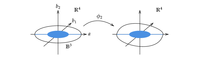
The special case treated by Theorem 5.1 is more readily visualized than the general case. We illustrate the essential ideas in Figure 3 and Figure 4 below.
Proof.
We aim to extend to a continuous mapping , so that the degree of can be computed from the degree of . The extension is accomplished in stages, building up from dimensions to . For that purpose, we write
Similarly, means .
Start by letting be the identity mapping on , that is, whenever , which is consistent with the second equation in ((7)). Also let be the identity on the -dimensional upper halfball of radius . (We use “” subscripts to refer to the upper half of an object and “” for the lower half.) In particular, .
Step 1 — extend to upper half -ball. In this step and the next, we aim to extend continuously to the -dimensional ball in such a way that the extension still satisfies the reflection symmetry equation and vanishes only at the origin. We start by extending to the upper half of the ball.
Consider the annular region and its upper half
The boundary of (as a domain in ) decomposes into three parts: , and , which we call the outer, inner, and bottom boundaries, respectively. We have already chosen to equal the identity on the inner and bottom boundaries, and since by hypothesis equals the identity on the unit circle where the outer boundary meets the inner one, we see that is continuous on the whole boundary . Remember also that on the outer boundary.
Take to be any continuous extension of that is smooth on . For example, we could choose on to be the harmonic extension of the boundary values , meaning the we extend each of the four components of harmonically. Since does not vanish on , we know the boundary image does not contain the origin. Hence attains a positive minimum value on , and so for some sufficiently small , the image does not intersect the ball . Thus the preimage is separated from the boundary, meaning there exists such that
| ((8)) |
Step 2 — eliminate zeros and extend to lower half -ball. The map might have zeros in . To eliminate them, we perturb the map as follows and then extend to . See Figure 3.
The -dimensional domain is mapped smoothly under into . The image has zero -dimensional volume, and so does not contain the ball . Thus we may take a point . Define a perturbed mapping on by
This perturbed mapping is continuous, since the distance function is continuous and equals on . Further, equals on , and in particular equals the identity on the upper halfball .
This construction ensures that when , as we now show. The claim is immediate if since then , which is nonzero because . And if then , while by ((8)), and so
Now that we have extended to on the upper halfball in dimensions, we may extend to the lower halfball by defining
| ((9)) |
when , that is, when , and with . This definition ensures that satisfies the reflection symmetry property ((7)) for all with (equivalently, with ). Also, equals the identity mapping on the lower halfball of radius , because if then the definition gives that
since equals the identity on the upper halfball of radius . Similarly, on the lower half-sphere , since on the upper half-sphere and both and satisfy reflection symmetry.
We must verify that the extended map is continuous on the set where the upper half of the -ball joins the lower half. Since , the reflection acts on simply by changing the sign of the first coordinate. Thus the extended definition ((9)) says
where
flips the sign of the first and third coordinates in . Suppose with . If and then
Thus is continuous on the joining set , and so on all of .
Step 2 is complete: we have found a continuous mapping of into that satisfies there the reflection symmetry property ((7)), agrees with on the sphere , equals the identity on , and is nonzero except at the origin.
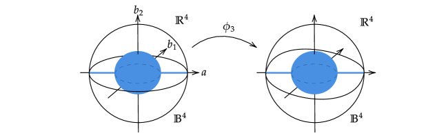
Step 3 — extend to -ball. The next task is to extend continuously to the -dimensional ball while preserving reflection symmetry and ensuring the extension equals on . Figure 4 summarizes the extension process.
First extend to be the identity map on the upper halfball of radius , and define to equal on . Consider the annular region
and its upper and lower halves
Choose to be a continuous extension of to the upper halfball. For example, we could harmonically extend the components of from into the interior of . Further extend to the lower halfball (which contains ) by defining
| ((10)) |
This definition ensures that satisfies the reflection symmetry property ((7)) on the ball . (We already knew that property on , by the previous step.) Further, equals the identity mapping on the lower halfball of radius , because if then
since is the identity on . Similarly, reflection symmetry for and guarantees that on the lower half-sphere , since on the upper half-sphere by construction.
We still need to verify continuity of on the set where the upper half of meets the lower half. Suppose with and . We consider two cases. First, if then and so the definition gives
by reflection symmetry for . Second, if then and so
since is the identity on by construction. Hence
| by ((10)) | |||
| since reflections preserve norms | |||
| since is the identity on | |||
by uniform continuity of on (recall ). Thus in both cases, is continuous at .
Step 4 — compute degree by decomposition of -ball. The ball has disjoint decomposition
where
Notice is nonzero on by construction in Steps 2 and 3. Removing from the ball preserves the degree, by the excision property [2, Theorem 2.7], and so . Then the domain decomposition property of degree [2, Theorem 2.7] implies
since equals the identity on . Hence , which finishes the proof of Theorem 5.1. ∎
The next lemma was used above in the proof of Theorem 5.1. It is a special case of [11, Lemma 17] (take there). Several computations used in the proof in [11] are eliminated in the new and shorter proof below, by introducing a deformation .
Lemma \thelemma (Reflection symmetry and degrees on the half-annuli).
Let and be the upper and lower annular regions of . If is a continuous map satisfying the reflection symmetry property (7) and is nonzero on then the degrees on the half-annuli sum to zero:
Proof.
Since does not vanish where (note such points lie on the boundary of ), we may choose sufficiently small that does not vanish when . The excision property of degree allows us to truncate the half-annuli without changing the degrees, namely omitting all points with and concluding that where
The goal is now to show .
On we have and so , and hence
by the reflection symmetry property (7). Let
so that and . Clearly because its second coordinate is greater than or equal to .
Define a homotopy by
for , where we note that the right side is well defined since . The definition ensures . Further, is nonzero on since is nonzero on . Hence homotopy invariance of degree [2, Theorem 2.3] yields that
On the right side of this formula, observe that
By the multiplicative property of degree [2, Theorem 2.10], the reflections on the range each multiply the degree by , and so do the reflections and that preserve the domain and the reflection that maps to . These five reflections together multiply the degree by , and so
Combining the equalities and recalling that , we conclude as desired that
∎
Acknowledgments
Kim is supported by an RTG grant from the National Science Foundation (#2135998). Laugesen’s research is supported by grants from the Simons Foundation (#964018) and the National Science Foundation (#2246537).
Appendix A The Robin problem on the unit disk
The trial function constructed in ((2)) involves the second Robin eigenfunction of the unit disk, whose properties we now summarize. The disk eigenfunctions satisfy
where for simplicity we do not rescale the Robin parameter by like in Theorem 1.1. The parameter range in that theorem corresponds to in this appendix. For a plot of the Robin eigenvalues of the disk as a function of , we recommend [7, Figure 4.2].
Proposition \theproposition (Second Robin eigenfunctions of the disk).
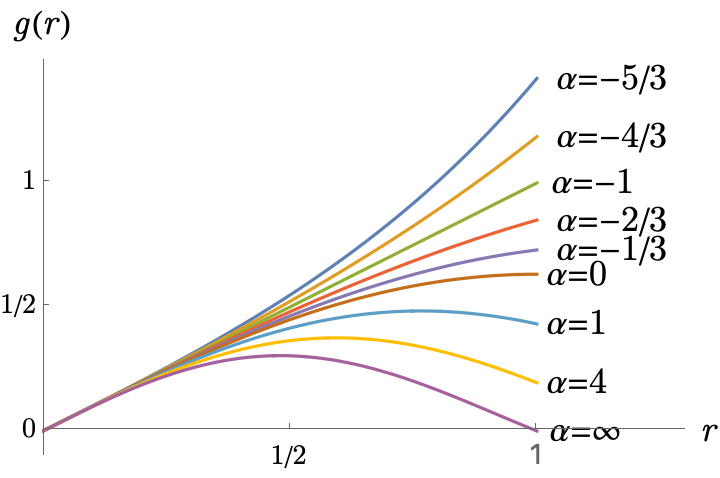
Let . A complex-valued eigenfunction for , can be taken in the form where the radial part has for , and . When , is strictly increasing and . When , is initially positive and then negative.
The eigenvalue is negative when , equals zero at , and is positive when .
The second eigenvalue of the disk has multiplicity since yields both a sine and cosine mode. Thus the second and third eigenvalues agree.
The second eigenvalue can be evaluated in terms of the Bessel function , when . We will not need the formula in this paper, but for the sake of completeness we recall (see [4, Section 5] with dimension ) that where is the smallest positive solution of the Robin condition .
References
- [1] D. Bucur and A. Henrot, Maximization of the second non-trivial Neumann eigenvalue, Acta Math. 222 (2019), 337–361.
- [2] I. Fonseca and W. Gangbo, Degree Theory in Analysis and Applications. Oxford Lecture Ser. Math. Appl., 2. Oxford Sci. Publ. The Clarendon Press, Oxford University Press, New York, 1995.
- [3] P. Freitas and R. S. Laugesen, From Steklov to Neumann and beyond, via Robin: the Szegő way, Canad. J. Math. 72 (2020), 1024–1043.
- [4] P. Freitas and R. S. Laugesen, From Neumann to Steklov and beyond, via Robin: the Weinberger way, Amer. J. Math. 143 (2021), 969–994.
- [5] A. Girouard and R. S. Laugesen, Robin spectrum: two disks maximize the third eigenvalue, Indiana Univ. Math. J. 70 (2021), 2711–2742.
- [6] A. Girouard, N. Nadirashvili and I. Polterovich, Maximization of the second positive Neumann eigenvalue for planar domains, J. Differential Geom. 83 (2009), 637–661.
- [7] A. Henrot, ed. Shape Optimization and Spectral Theory. De Gruyter Open, Warsaw, 2017.
- [8] J. Hersch, Quatre propriétés isopérimétriques de membranes sphériques homogènes, C. R. Acad. Sci. Paris Sér. A-B 270 (1970), A1645–A1648.
- [9] M. Karpukhin and D. Stern, Min-max harmonic maps and a new characterization of conformal eigenvalues, J. Eur. Math. Soc. (JEMS) 26 (2024), 4071–4129.
- [10] H. N. Kim, Maximization of the second Laplacian eigenvalue on the sphere, Proc. Amer. Math. Soc. 150 (2022), 3501–3512.
- [11] H. N. Kim, Upper Bound on the second Laplacian eigenvalue on real projective space, ArXiv:2401.13862.
- [12] R. S. Laugesen, The Robin Laplacian — spectral conjectures, rectangular theorems, J. Math. Phys. 60 (2019), 121507.
- [13] R. Petrides. Maximization of the second conformal eigenvalue of spheres, Proc. Amer. Math. Soc. 142 (2014), 2385–2394.
- [14] G. Szegő, Inequalities for certain eigenvalues of a membrane of given area, J. Rational Mech. Anal. 3 (1954), 343–356.
- [15] H. F. Weinberger, An isoperimetric inequality for the -dimensional free membrane problem, J. Rational Mech. Anal. 5 (1956), 633–636.