Constraints from Entanglement Wedge Nesting for Holography at a Finite Cutoff
Abstract
We explore constraints that arise from associating an entanglement wedge (EW) to subregions of a cutoff boundary at a finite distance in AdS/CFT, using a subcritical end-of-the-world (ETW) brane acting as the cutoff.
In particular, we consider the case of two intervals in the holographic dual to a BCFT, with one interval located at the asymptotic boundary and the second interval located on the ETW brane. We discuss in detail subtleties that arise near the RT end-points when defining the EW for this configuration, particularly in the connected phase. Entanglement wedge nesting (EWN) requires that . We demonstrate that already in the simplest example of an AdS3 bulk geometry, EWN can be violated even if and are spacelike separated through the bulk and instead we must require the stronger condition that be spacelike separated from , which highlights the non-local nature of the cutoff theory. Our prescription to associate EWs to subregions on the ETW brane is different from the restricted maximin procedure Grado-White:2020wlb but will agree within the subset of parameter space where EWN is respected.
Additionally, we study EWN in a two sided BTZ black hole geometry with an ETW brane in one of the exteriors. In the BTZ black hole example we find that our condition for EWN disallows configurations where the RT surface goes from the brane to the black hole singularity.
1 Introduction
1.1 Motivation and Background
While the AdS/CFT correspondence Maldacena:1997re ; Witten:1998qj ; Gubser:1999vj ; Nastase:2007kj ; Polchinski:2010hw ; Ammon:2015wua ; VanRaamsdonk:2016exw is our best model of holography to date, it is – in its best established form – limited to describing a gravitational theory in an asymptotically AdS spacetime with prescribed boundary conditions at infinity Witten:1998qj ; Gubser:1998bc ; deHaro:2000vlm . This presents a significant obstacle for studying quantum gravity in more realistic flat or de Sitter backgrounds, as well as localized subregions.
One attempt at generalizing the duality between quantum gravity in a bulk AdS spacetime and a quantum field theory on the asymptotic boundary is to consider spacetimes with boundaries at a finite proper distance. Understanding holography in such a setting would enable to study quantum gravity in finite local subregions, but also to potentially embed cosmologies in holography Gubser:1999vj ; Cooper:2018cmb . More generally, such ideas can be understood in the framework of the surface/state correspondence Miyaji:2015yva ; Miyaji:2015fia , which assigns a quantum state to convex codimension-two submanifolds in a gravitational spacetime.
Concrete realizations for the surface/state correspondence can be found, apart from tensor networks which motivated the correspondence, for example in the study of -deformations of holographic CFTs Zamolodchikov:2004ce ; Jiang2019LecturesOS ; Bonelli:2018kik ; Dubovsky:2017cnj ; Grieninger:2019zts ; Gross:2019ach ; Cavaglia:2016oda . It has been proposed that a deformation of a holographic CFT should be understood as “moving the boundary into the bulk” McGough:2016lol ; Guica:2019nzm ; Lewkowycz:2019xse . Furthermore, the appearance of cutoff surfaces have also played a key role in double holography Takayanagi:2011zk ; Almheiri:2019hni ; Chen:2020uac ; Chen:2020hmv ; Hernandez:2020nem ; Grimaldi:2022suv ; Neuenfeld2021DoubleHA ; Neuenfeld:2021wbl ; Omiya:2021olc ; Geng:2023iqd , where a convex cutoff surface in the form of an end-of-the-world (ETW) brane appears. Doubly-holographic models with AdS branes start by introducing the dual of a holographic -dimensional boundary BCFT in terms of a -dimensional bulk AdS spacetime.111BCFTs are conformal field theories living on a space with boundary at which conformal boundary conditions are imposed. However, at least for a BCFT2 one needs to introduce boundary degrees of freedom which break conformal invariance in order to obtain interesting models, e.g. by coupling an SYK model to the BCFT boundary. We will will thus use the term BCFT more loosely to also account for situations like this. The boundary of the BCFT is continued into the bulk by an ETW brane Takayanagi:2011zk which removes part of the naive bulk spacetime dual to a CFT without boundary.
Naturally, it is tempting to extend lessons learned from AdS/CFT to holography at a cutoff. Of particular interest are holographic computations of entanglement entropies. In AdS/CFT the holographic entanglement entropy of some subregion of the asymptotic boundary is given, at leading order in , by the Hubeny-Rangamani-Ryu-Takayanagi formula222In fact, in certain situations such as black hole evaporation, the quantum corrected RT formula Engelhardt:2014gca can yield results that differ at leading order from the RT formula. We will not be concerned with such situations in this paper. Ryu:2006bv ; Hubeny:2007xt
| (1) |
where is the the minimal area extremal surface homologous to the boundary subregion . The surface is known as the HRRT surface or RT surface for short.
The surface/state correspondence proposes that in the case of a finite cutoff the von Neumann entropy of a reduced density matrix obtained from can be computed from co-dimension two extremal surfaces that are anchored at the boundary of subregions of (a slice of) the spacetime boundary . A basic consistency check of this proposal with holographic subregion entropy computations has e.g. been performed in the context of in Donnelly:2018bef . Also in double holography, there is evidence that subregion entropies on the brane can be computed using the RT formula Chen:2020uac . However, it is still unknown under which conditions the proposal of the surface/state correspondence is fully consistent. While it is not even clear what “consistency” entails in detail, strong subadditivity (SSA) of holographic entanglement entropy Headrick:2007km ; Wall:2012uf should certainly be a necessary condition if we want the holographic entanglement entropy to behave like an entropy in the quantum information theoretic sense.
In addition, in standard AdS/CFT we have a notion of subregion/subregion duality Headrick:2014cta ; Akers:2016ugt ; Akers:2017ttv ; Chen:2021lnq ; Leutheusser:2022bgi . More precisely, a boundary subregion is dual to the entanglement wedge which is defined as the causal past and future of the partial bulk Cauchy slice bounded by and the corresponding RT surface . Moreover, given a subregion , is dual to which must be a subset of . This follows from the fact that tracing out parts of to acts as a quantum channel on the reduced density matrix . This property of entanglement wedges is called entanglement wedge nesting (EWN).
The purpose of this paper is to first carefully describe the subtleties in defining entanglement wedges for cutoff subregions , and second, to the non-trivial conditions on the relative location of with respect to another subregion (disjoint from ) imposed by EWN. For concreteness, we will focus on the simplest geometry which allows for non-trivial statements, namely AdS3 and Planar BTZ cut off by a hyperbolic ETW brane. Throughout this paper, we will take the perspective that one can freely choose a subregions and in much the same way as one can choose a subregion on a standard holographic boundary.333The reader should be cautious to not confuse this with the closely related notion of islands. Although the case of finding islands occurs in the connected phase the issue of knowing where on the brane the extremal surface is anchored is dynamically determined as part of the extremization problem. In our case we are considering fixing a brane region and fixing a boundary region independently. In a certain sense we are considering Dirichlet boundary conditions on the brane whereas island setups use Neumann conditions. However, the theory on the cutoff surface might in general be gravitational as is the case in doubly holography Karch:2000ct . This naively poses the question of how to define cutoff subregions in a diffeomorphism invariant way. In this paper, we restrict ourselves to the strict limit, such that gravity is effectively turned off in the bulk. In this case subregions can be defined uniquely.444The authors of Bousso:2022hlz proposed the notion of generalized entanglement wedges for gravitational theories. Their proposal only works for subregions of a time-reflection symmetric Cauchy slice and thus is not applicable to our configurations. Extending this discussion to corrections, while interesting, will not be pursued here.
We will assume that the RT formula in its simplest formulation, Eq. (1), holds. Given this starting point, the RT surface which computes for two disconnected, spacelike subregions and consists of two disconnected pieces which can be in one of two phases. Either, each connected piece can be homologous to one of and . In this case, which we will call the disconnected phase, the mutual information vanishes. The second phase has the RT surface connect the subregions and to each other. Consequently, the mutual information does not vanish. We will call this the connected phase. We will then construct the entanglement wedges for the regions , , and . As we will argue below, while the definitions of and are straight forward and agree with the intersection of entanglement wedge in the full geometry cut off by the brane, the definition of the connected entanglement wedge is more subtle and requires us to be careful about the location and direction at which the RT surface ends on the cutoff surface.
We find that, in general, and unlike AdS/CFT, spacelike separation of and is not enough to ensure EWN. As we will argue, this happens because spacelike separateness of and , while sufficient to make sure that each connected piece of the associated RT surfaces is spacelike, is not enough to guarantee that the disconnected pieces of the RT surfaces are also spacelike separated. What we demonstrate is that the non-trivial condition EWN imposes precisely ensures that all the disconnected pieces of the RT surfaces are spacelike separated. Requiring that EWN is satisfied imposes a bound on the relative separation of and which is stronger than spacelike separation through the bulk.
It is well known Lewkowycz:2019xse ; Geng:2019ruz ; Grado-White:2020wlb ; Neuenfeld:2023svs that naively extending in HRT formula for cutoff surfaces can yield situation where SSA and EWN is violated. This motivated the authors of Grado-White:2020wlb to propose a modification of the RT formula for cutoff surfaces, called restricted maximin. The main idea of their proposal is to only consider bulk extremal surfaces which lie on a Cauchy slice that intersects , which guarantees SSA and EWN. However, as we will argue below, applying their construction to a configuration of disjoint subregions and which violate our bounds will produce RT surfaces which disagree with naive expectations. For example, given a static geometry and subregions and on constant but different time-slices, the two disjoint components of the RT surface in the disconnected phase will have a non-trivial profile in time. Since this happens whenever and are timelike separated, this suggests that a deviation between the naive RT surfaces defined in this paper and restricted maximin surfaces indicates that and are not independent, possibly due to the non-local nature of the theory at the cutoff.
1.2 Overview
This paper is roughly divided into two parts. The first part consists of Sections 2 and 3 where we explore EWN in Poincare AdS3 cutoff by an end-of-the-world (ETW) brane. In the second part of this work, given in Section 4, we study EWN for a two-sided planar BTZ black hole geometry with the right exterior cutoff by an ETW brane.
More specifically, in Section 2 we consider two disjoint spacelike separated constant time intervals and on the conformal boundary and brane respectively. Identifying the RT surfaces that we will use in our prescription which are homologous to , , and we define entanglement wedges , , and respectively. We address the subtle aspects of correctly identifying the entanglement wedges for brane subregions, which involve finding spacelike separated regions from the relevant RT curve line segments. When we explicitly construct we show that the RT surface that is homologous to can generally be extended behind the brane and will be homologous to a subregion on the “imaginary” or “virtual” conformal boundary behind the brane, which we denote as . By defining an “entanglement wedge”, denoted as , in the extended spacetime we demonstrate that , where is the physically relevant portion of the spacetime in front of the brane. However, when constructing in the connected phase, we demonstrate that it is generally not possible to view as the intersection of some kind of extended wedge with .
In Section 3 we explore whether EWN (i.e., requiring that ) places non-trivial constraints on the relative placement of the spacelike separated intervals and . We derive the necessary and sufficient condition on the set of parameters that define the location of and to ensure that the EWN is satisfied when is in the connected phase (see Eq. (43)). We show that the condition to satisfy EWN amounts to ensuring that the RT surfaces homologous to , , in the connected phase are all spacelike separated from each other. We conclude our exploration by emphasizing that in our setup we must non-trivially require that and be spacelike separated, which is a stronger condition in cutoff holography than simply requiring that and be spacelike separated. We connect this back to the expectation that holographic theories on cutoff surfaces are generally expected to exhibit a certain degree of non-locality and that our results corroborate this expectation. We also comment on how our results and prescription for defining entanglement wedges of subregions on cutoff surfaces compare to the restricted maximin prescription, which necessarily gives rise to entanglement wedges that respect EWN. We argue that the RT surfaces used in our prescription and the maximin prescription agree within the subset of parameter space where we EWN is satisfied (i.e. when all the relevant RT surfaces are spacelike separated).
In Section 4 we study EWN in a two-sided planar BTZ black hole background whose right exterior is cutoff by an ETW brane. We introduce the intervals and on the brane in the right exterior and on the boundary in the left exterior, respectively. We discuss the RT surfaces that will be homologous to the subregions , , and and use them to define the entanglement wedges , , and respectively. Using similar methods employed in the first part of the paper in AdS3 we can write down the condition that needs to be placed on the intervals and so that in the connected phase. We find that in the limit where the brane and boundary interval lengths diverge the condition has a simple geometric interpretation in the bulk. This interpretation is that requiring EWN in the connected phase prevents the connected RT surfaces from touching the black hole “singularities” at Kruskal time . This provides an interesting result in the context of Lee:2022efh which also analyzed the same BTZ black hole setup to constrain DGP couplings (more specifically the gravitational coupling set by the value of a JT dilaton) on the brane. The result we obtain serves as another reason beyond the ones discussed in Lee:2022efh to ignore RT surfaces that cross the “singularities” at .
We conclude the work in Section 5 where we summarize the main results and ideas of the paper and discuss future avenues of exploration.
2 Constructing Entanglement Wedges in AdS3 cutoff by ETW Brane
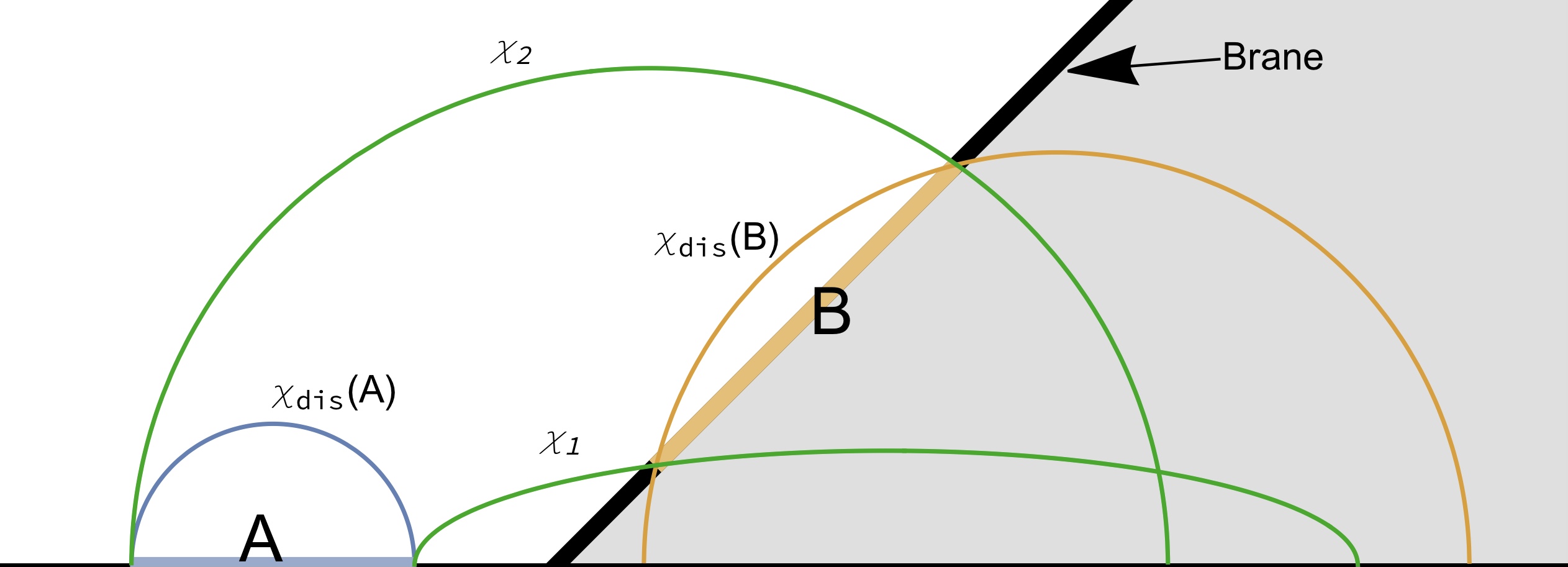
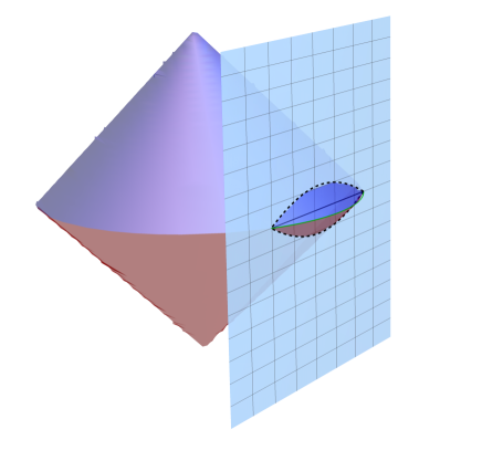
In this section, we will present a prescription to construct entanglement wedges in AdS3 with an ETW brane acting as a cutoff surface. We will fix spacelike subregions and on the boundary and brane, respectively, and then consider candidate extremal surfaces that are homologous to , , and , which we denote as , and , which we depict in Figure 1. These extremal surfaces are then used to construct entanglement wedges , , and which will later be used to study EWN.
Section 2.1 briefly reviews ETW branes in Poincare AdS3. Explicit expressions for relevant RT surfaces are given in Section 2.2. In Section 2.3 a classification of the extremal surfaces is given in terms of conic sections and we show that due to the presence of the ETW brane a larger set of surfaces than in standard holography must be considered. In Section 2.4 we describe how our entanglement wedges are constructed and also provide explicit examples. Through our construction we demonstrate that while can be thought of as naively being cut out of a larger wedge in the extended spacetime, this is generally not possible for , since our prescription and the naive extended wedge prescription will differ near the brane.
2.1 AdS3 Poincare Patch with an ETW Brane
Our starting point is AdS3 in Poincare coordinates,
| (2) |
where is the AdS radius, is the radial bulk coordinate and is the conformal boundary which is parameterized by .
The ETW brane is a co-dimension one surface in the bulk which satisfies the the metric equation of motion of the Lorentzian action555Note in our setup in Poincare AdS the boundary of the bulk cutoff by the brane consists of the conformal boundary as well as the ETW brane so we should also include a Gibbons-Hawking term of the form . For simplicity we omit explicitly writing it this in the action and focus on the brane and bulk terms. Takayanagi:2011zk
| (3) |
The parameter denotes the tension of the ETW brane. Varying Eq. (3) with respect to the metric gives an equation that needs to be satisfied by the brane,
| (4) |
where is the induced metric on the brane and is the extrinsic curvature. We can rewrite the equation above into a more simple form by substituting its trace,
| (5) |
It is straightforward to check that in Poincare coordinates the solution for an ETW brane that intersects the conformal boundary at is given by
| (6) |
where is a parameter that is related to the brane tension via . When the tension is zero the ETW brane cuts off half of the AdS space and when the ETW brane coincides with the conformal boundary. The limit of , i.e., the limit in which the brane approaches the “would be conformal boundary” is referred to as the critical limit. The critical limit is physically relevant in the discussion of gravity induced on the brane, particularly in higher dimensions. It is a limit in which bulk gravitons become localized on the brane and one can consider a conventional lower dimensional gravity theory on the world volume of the brane Karch:2000ct ; Geng:2020qvw ; Neuenfeld:2021wbl . In the three-dimensional case discussed here, a theory of dilaton gravity gets induced on the brane, and the critical limit is the limit in which the cutoff scale of the brane theory becomes small Neuenfeld:2023svs .
Throughout this work we will denote as the remaining spacetime after the cutoff is introduced. In the case of AdS3 cut off by an ETW brane whose position is given by Eq. (6) we can explicitly express as
| (7) |
where is the Heaviside step function. The metric on is identical to AdS3 with the only difference being that the ETW brane cuts off a the portion of AdS3 which is “behind” the brane.
2.2 Candidate RT Surfaces in AdS3 with an ETW Brane
We consider two constant time subregions, and living on the boundary of this spacetime. is an interval with at time on the conformal boundary at . Subregion lives on the brane at time . It is located at for and such that . The proper length of this interval is given by .
Since in our approach the RT surfaces by definition are the minimal extremal surfaces homologous to regions and , we now need to consider the different extremal surfaces which are anchored to those subregions. Since the bulk is three dimensional the extremal surfaces are curves that extend through the bulk. We parameterize these curves in terms of the Poincare coordinate and extremize the area functional
| (8) |
where and . The general solutions to the equations of motion associated with the functional in Eq. (8) are given by (see Appendix A.1)
| (9) |
The four undetermined constants, can be expressed in terms of the coordinates , , , , which determine the entangling surfaces.
There are two possible configurations of the extremal surfaces. Either, the extremal surface consists of two disconnected pieces which are separately homologous to and . We will denote those surfaces by , , respectively, where the subscript stands for disconnected. Explicitly, is given by
| (10) |
This is simply a semi-circle of radius centered at on the constant plane. Similarly, is given by
| (11) |
This curve is a section of the semi-circle whose radius is given by centered at on the constant plane. In particular, we can think of it as an RT surface which ends on an interval of the asymptotic region in the nonphysical region of spacetime behind the brane, which intersects the ETW brane at the boundary of .
The other configuration consists of two line segments which connect to and to . We will denote those two surfaces by and , respectively, and call their union the connected surface666The fact that the connected RT surface consists of two disconnected segments is special to and we hope that this naming convention will not be the source of confusion. . The explicit trajectories are given by
| (12) | ||||
where and .
2.3 General Classification of Extremal Surfaces in Poincare AdS3
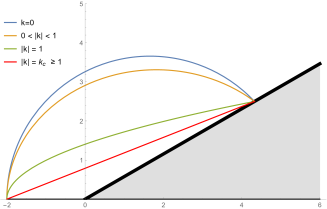
In our setup, RT surfaces are conic sections in the -plane. In the special case where the endpoints lie on the same constant time-slice, they are half circles. However, more generally RT surfaces have a slope in time direction , c.f. Eqs. (9) and (12), such that the projection on the -plane is one of the three conic sections (ellipse, parabola, or hyperbola). Which of the three sections is realized depends on the value of ,
| circle | ellipse | parabola | hyperbola |
In usual AdS/CFT, i.e. when the spacetime boundary is at asymptotic infinity, one only considers RT curves that have (i.e. circles and ellipses), since all the extremal surfaces have to end on the boundary. RT surfaces with may start on the asymptotic boundary at but never return. However, in the presence of a cutoff, such as the brane under consideration, we can now attach one endpoint of the extremal surface to the brane for which generally . This allows for novel configurations where the RT curve has .
Nonetheless, for above a certain threshold, the extremal surface becomes timelike. Here, we consider only spacelike separated points with respect to the bulk metric, as expected in computations of entanglement entropy for spacelike separated subregions.777For work on timelike entanglement entropy see Doi:2022iyj ; Liu:2022ugc ; Doi:2023zaf ; Li:2022tsv . In this case we have that , where and are the coordinate distances between the RT endpoints. This places an upper bound on the parameter , with given by
| (13) |
The value is special to our model and arises from maximizing over all boundary and brane points. Restricting the RT surface to end on the asymptotic boundary of course reproduces the situation in standard AdS/CFT with . In the limit where the line segment becomes a null geodesic (i.e. a straight line in the -plane). We depict several configurations in Figure 2.
Before continuing, it is important to note that in the definitions of , , and , Eqs. (10) – (12), we have restricted the range of the parameter along the curves so that they would lie within . For our future discussions it will also be useful to define the extension of these extremal curves so they are not only defined in but also in AdS3 which includes the region “behind” the brane, shaded in gray in Figs. 1 and 2. This is achieved by simply lifting the restrictions on the parameter and continuing the expressions into the region behind the brane. We will distinguish these extended extremal curves with a bar on top of the . For example, the extension of is given by and it is straightforward to see in this definition that .
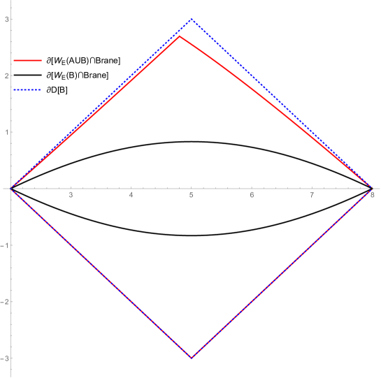
Fig. 1 shows an example of the boundary and brane subregions along with the associated extremal surfaces in the -plane. The shaded gray region is the portion of AdS that is cut off by the ETW brane and is not physically relevant in our discussion. The blue curve and the yellow curve are half-circles. The union of the green line segments form the connected surface, . In this particular case the two line green line segments correspond to ellipses in the -plane.
2.4 Constructing the Entanglement Wedges
Once the candidate RT surfaces are known, we can construct the associated entanglement wedges. In standard holography, the entanglement wedge is defined by taking a boundary subregion together with its associated RT surface . One then considers a partial Cauchy surface, , whose boundary is given by . The entanglement wedge of the boundary subregion , denoted , is then given by the domain of dependence of the partial Cauchy slice . It is tempting to suggest that to construct the entanglement wedge to an associated boundary region one can simply define an extended entanglement wedge using and then cut off the extended wedge with brane and identify the remaining portion in as . As we shall see in our discussions, such a prescription is generally not valid in the cases where our boundary subregions lie on cutoff surfaces such as the brane.
The explicit construction of the entanglement wedge of an interval on the conformal boundary can be understood by introducing a null congruence orthogonal to the RT surface, which is directed towards the past and future towards the boundary. In the case of a simple geometry like Poincare AdS3 it is straightforward to show that the null sheets generated by this family of null geodesics are light cones whose coordinate description is very simple. In particular, in our setup for the interval , one finds that is given by the points which satisfy
| (14) |
see Fig. 3 for an illustration. Now let us define as a partial Cauchy slice whose boundary is given by . Any future(past) oriented causal curve going through a point to the past(future) of within the wedge enclosed by the light cones will eventually intersect and for any point outside the light cones one can find a causal curve that does not go through . This means that the region enclosed by the light cones really is the domain of dependence of which by definition means it is .
In our setup we also have spatial boundary subregions that (at least partially) live on the brane, namely and . We already know that the RT curves associated with and are given by and respectively. We define the entanglement wedge of the subregion denoted, , as the domain of dependence of the partial Cauchy slice whose boundary is given by . In a similar manner we define the the entanglement wedge of subregion , denoted , as the domain of dependence of the partial Cauchy slice whose boundary is given by , where we remind the reader that and are the extremal surfaces which connect the boundaries of and .
The challenge now is to characterize the set of points in and . In the case of the boundary interval we can find by simply considering the set of spacelike separated points from towards the boundary and this naturally gives rise to the light cones bounding the entanglement wedge. In a similar manner is the set of spacelike separated points from going towards the brane.
As for we will consider the region which is given by the intersection of points that are spacelike separated from towards with the points that are spacelike separated from towards in . This will trace out a tube-like region through the bulk which will connect interval to interval . In standard AdS/CFT this would give the domain of dependence of the partial Cauchy slice in the connected phase. As we will see in the next section, the situation is more complicated in the presence of a cutoff.
To explicitly characterize the spacelike regions of interest in we need to identify spacelike separated points from curve segments in AdS3. Understanding the subtleties of doing this will be the primary aim of the discussions in Subsection 2.4.1. We will then explicitly construct in Subsection 2.4.2 and in Subsection 2.4.3. Note that much of the explicit construction that is discussed in this subsection is not required to formulate the conditions for EWN in Section 3. Here we present the construction for the sake of completeness of the discussion of the various entanglement wedges that are involved in our setup and to illustrate subtleties in defining entanglement wedges in the connected phase.
2.4.1 Spacelike Separated Points from RT Curves in Poincare AdS3
To understand the entanglement wedge of various brane-boundary subregions it is essential to characterize which points in the bulk are spacelike and timelike separated from the RT surfaces. We can identify the regions for extremal line segments through the methods discussed in Appendix A.2. We summarize the procedure in the following.
Suppose we have an extremal line segment, , parameterized in terms of the Poincare coordinate (i.e. we have a curve and ). At the endpoints of the line segment we introduce planes that are orthogonal to the tangent vectors,
| (15) |
where and . The subscripts indicate that the planes correspond to the endpoints at smaller or bigger which are left and right in our figures. As we work through explicit examples these regions will become more clear. The normalized unit tangent vector to the left and right endpoints, which we denote as and respectively, take the form
| (16) |
Since is a unit normal vector to the plane we can use it to characterize which “side” of the plane we are on. For any point we can take a line segment orthogonal to that connects a point on denoted as to that satisfies . Based on this, we say is to the in the direction of () from if (). Using this terminology, we define to be the set of bulk points that are in the direction of from . We define , , and .
In the region the set of spacelike separated points from the extremal curve can be understood by emitting null geodesics orthogonally from each point on the curve. We will refer to the null sheet generated by emitting null geodesics orthogonally from the “null evolution” of denoted . The points outside the null evolution of are spacelike separated from .
In the region the set of spacelike separated points can be understood as being outside the light cones emitted by the endpoints of the extremal surface. These are the points that will satisfy the following inequality .
Importantly, in general, if we have an extremal surface that lives in AdS3 and another extremal surface , the set of points in which are spacelike separated from will generally differ from the set of spacelike separated points from due to the finite extent of the extremal surfaces.
In particular, one could naively extended all extremal surfaces behind the brane, , and defined spacelike separation in the physical spacetime as the restriction of spacelike separation in the extended spacetime to points in . As we will see in Section 2.4.2, our approach and this naive approach will correctly identify . However, when constructing in the connected phase in Section 2.4.3 the naive approach will not correctly give the entanglement wedge. It is also worth mentioning that if one defines an extended wedge in the extended spacetime using we know by construction that null sheet enclosing will always fully enclose a co-dimension 0 region between and the brane. However, it is possible for portions of the null sheet in front of the brane to be generated by geodesics that originate from behind the brane. Our prescription relies only on null rays emitted from . In fact, we can say that the entanglement wedge can be correctly identified using the naive prescription iff the null sheet which encloses can be completely generated by null congruences emitted from . Such is the case for but not for .
2.4.2 Construction of
By definition is the set of points that are spacelike separated from towards the brane. In our case, it is relatively straightforward to explicitly construct . We can define the regions by introducing the planes given by,
| (17) |
and given by,
| (18) |
Making use of the notation discussed immediately after Eq. (16) we can define and describe . In particular, can be intuitively understood as the region wedged between and . The region can be understood as being between the planes and (i.e. to the “left” of ). In a similar manner is the region between the planes and (i.e. to the “right” of ). We adopt the notation to denote the set of spacelike separated points to in the subregion . Using this notation we can write888We obtain the definition of from Eq. (LABEL:SLTowardsBdry) and Eq. (LABEL:SLAwayBdry) by setting and . The “” corresponds to the spacelike points towards the boundary and the “” corresponds to the set of spacelike points expanding away from the boundary.,
| (19) | ||||
| (20) | ||||
| (21) |
Due to the simplicity of out setup we can easily visualize all these regions together on various constant time slices. We depict them in Figure 4.
As time evolves, we can see that on each time slice a red curve encloses the RT curve line segment. This red curve is exactly the set of points that will be lightlike separated from at that particular time slice, and therefore the region outside the red curve is spacelike separated from . Another interesting point to make in this case is that the planes (the purple line in Figure 4) and (the blue line in Figure 4) intersect along a line on the conformal boundary behind the brane. By construction, this line is the axis along which the tips of the future and past cones intersect along . In fact, we can see as we approach the “shrinking” part of the null surface will converge at the apex of the boundary cones. What will be physically relevant for our discussion is the restriction to (i.e. the unshaded portion of Figure 4 above the thick black line representing the brane).
The points spacelike separated from towards the brane define . It is straightforward to see from Figure 4 that and that
| (22) |
In fact, one can understand the region as being cut from a larger entanglement wedge of a constant time slice interval that lives on the imagined, or virtual, asymptotic boundary behind the brane. This interval can be found by analyzing where intersects with the boundary this interval will be called . Using we can express the entanglement wedge of the brane interval, , as the intersection of the entanglement wedge of with the region of ,
| (23) |
The visualization of the points contained in the intersection is depicted in Figure 5, where the brane cuts out a small section of the larger wedge. The smaller piece the brane cuts is precisely .
To conclude the discussion of the construction of we should emphasize that we did not use the extension to define . The statement followed from our prescription. So in this special case, the naive approach of defining the wedge by cutting a piece out of a larger wedge and our approach match. However, we will see that when we construct the connected wedge in the next section, this nice coincidence between our approach and the naive approach fails.
2.4.3 Construction of
Now that we have identified the entanglement wedges associated with the boundary interval and brane interval we can consider the construction of the entanglement wedge associated with . In this case there are two possible phases that can exist for the entanglement wedge of . The disconnected phase, which is given by the union of the entanglement wedges discussed thus far (i.e. ). However, in the connected phase it is no longer true that the entanglement wedge is the union of the disjoint wedges. To determine in the connected phase we will adopt the procedure of finding the entanglement wedge through the prescription of finding the spacelike region away from the boundary from and the spacelike region toward the boundary for and then taking the intersection of those regions and restricting to . Roughly speaking, the region we will define will look like a “tube” that connects and regions on the brane-boundary system.
For each line segment we must begin by computing the relevant orthogonal planes. To begin, we note that both line segments and have their left endpoint on the conformal boundary so the planes for these points coincide for the conformal boundary and the region 999As we showed in Appendix A.2 the plane “” coincides with the boundary which implies that .. We only need to worry about for .
The orthogonal plane to at the the point where intersects the brane is denoted , where . The points on the plane satisfy
| (24) |
where , , and . Using we can define and using the notation/conventions introduced in Eq. (16). In this particular scenario, we will find as the region between the planes and and as the region between the planes and . Now we can define the set of spacelike points in each region
| (25) | ||||
| (26) |
We can then express the set of spacelike separated points in AdS3 from as .
In the special case where is a line segment with we can write more explicitly. This is because we can express in terms of light cones whose apexes are located at where
| (27) |
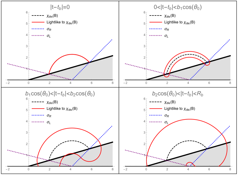
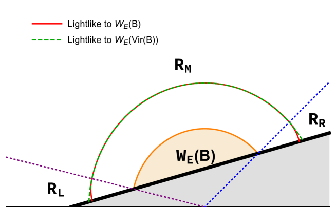
Using the discussion in Appendix A.4 along with the expressions given in Eq. (24) and Eq. (27) we can write down a formula for the null sheets emitted from in the special case where , which is given by Eq. (122). Using this we can generate Figure 6, which plots various time slices of the null sheets/congruences originating from the we depicted in Figure 1.
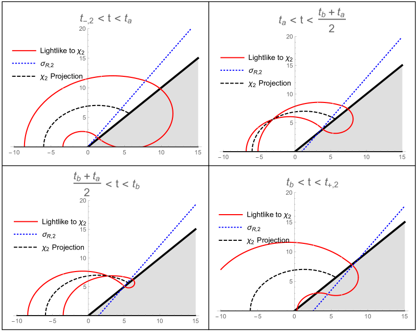
As in Figure 4, the red lines enclose the projection of (given by the dashed black line), although due to the nontrivial profile of over time, the red curve that surrounds the projection of takes on a more complicated shape. The blue dotted line is a time slice of the plane, , whose position changes over time, as we discussed. To the left of the dotted blue line the red line is obtained by the null evolution of , while to the right of the dotted blue line the red line is generated by a light cone centered at the point where ends on the brane. We can see how the red line segments are continuously glued along the plane in every time slice, as they should be through our construction.
In Figure 6, we consider 4 time regimes. The regime where the time slice is below the spacelike region on that slice is given by what is outside the red curve. The next two frames occur at time scales . In these regimes the constant time slice intersects with this occurs exactly at the point on the dotted black line (representing ) where the red lines appear to intersect along a “lobe”. We can see that this intersection point (“lobe”) moves along the as we shift the time slice in the window . The last frame depicts the time window when . Similar plots can also be obtained for as well, but they contain the same features, so we will not explicitly include them here.
It is worth noting that dotted blue line also allows us to identify the differences in our prescription for defining entanglement wedges and the naive prescription. In the naive prescription one would extend the RT surface behind the brane and compute the set of spacelike points to that extended curve and then restrict that to . On a given time slice the spacelike regions defined in the two prescriptions will match to the left of the dotted blue lines in Figure 6, but to the right of the dotted blue lines the spacelike regions will differ and so will the associated wedges.
Now that we have illustrated how we can find the set of spacelike regions from from we can use this to construct the in the connected phase. We start by considering where is the set of spacelike points from expanding “outward” towards and is the set of spacelike points from expanding “inward” towards . The intersection of the regions in will trace a smooth “tube-shaped” codimension 0 region enclosed by null sheets emitted from as long as and are spacelike separated from each other101010Unlike in standard holography, when we have a cutoff is not generally guaranteed to be spacelike separated from whenever and are spacelike separated. This fact will reappear in our discussions of EWN in Section 3.3.. Furthermore, we can postulate the existence of a specific partial Cauchy slice with boundary and we can identify the domain of dependence of with the set of points . For this reason we identify
| (28) |
In Figures 7 and 8, we consider an example to illustrate what the wedge will look like on various constant time slices. For each frame (constant time step) the brane is the thick black line. The remaining curves are color coded. Curves related to the line segment are green, and curves related to the line segment are blue. The dotted lines are the constant time slice of the planes which define the regions for each line segment. The dashed lines are the projections of on the constant time slices. The projection of the partial Cauchy slice is contained between the dashed lines. The solid green line is the set of lightlike points from evolving towards (spacelike points to are above the solid green line) and the solid blue line is the set of lightlike points from evolving towards (spacelike points to are below the solid blue line). On each time slice we line shade the region that is spacelike to both and and represents a constant time slice of .
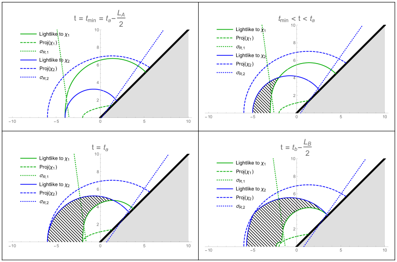
To get intuition on what the various frames in Figures 7 and 8 represent it is useful to remember the basic ideas behind the construction of . We take and emit null sheets outward towards and we consider another set of null sheets that are emitted from towards . The sheets emitted towards the “past” will intersect along a curve which we will call and the sheets emitted towards the future will intersect along another curve which we will denote . The region enclosed by these null sheets is precisely . and it will trace out a “tube.”
At time (Figure 7, top left frame) we see that there is no shaded region, this is because that time slice only contains the past tip of the causal diamond of on the conformal boundary which is represented by the intersection of the green and blue solid lines at the conformal boundary. In fact, this past apex is precisely where intersects with the conformal boundary.
In the next time frame (Figure 7, top right frame) we consider time scales in the window , we will begin to obtain slices of the connected wedge indicated by the line-shaded region. The intersection of the solid green and blue lines which pinch off the line-shaded region is the “past apex” of the entanglement wedge tube and will lie on the line .
At (Figure 7, bottom left frame) we can see that the connected wedge on the conformal boundary spans the entire subregion we can also see that the line-shaded region describing the connected wedge grows and the “past apex” (indicated by the intersection between green and blue solid lines) moves further along the curve towards the brane.
At time (Figure 7, bottom right frame), the line-shaded region becomes larger and develops “kinks” where it touches the projections of . These kinks were also seen in the discussion of Figure 6 and occur when the time slice intersects with and will persist at all times . Another important feature to mention on this time slice is that the intersection of the solid blue and green curve now occurs on the brane, and this is where the curve will terminate on the brane and this point represents the “past tip of the causal diamond” on the brane. We put “past tip of the causal diamond” in quotation marks because, in general, the intersection of the entanglement wedge with the brane will not be the naive causal diamond of the brane interval . So for all the curve will not appear.
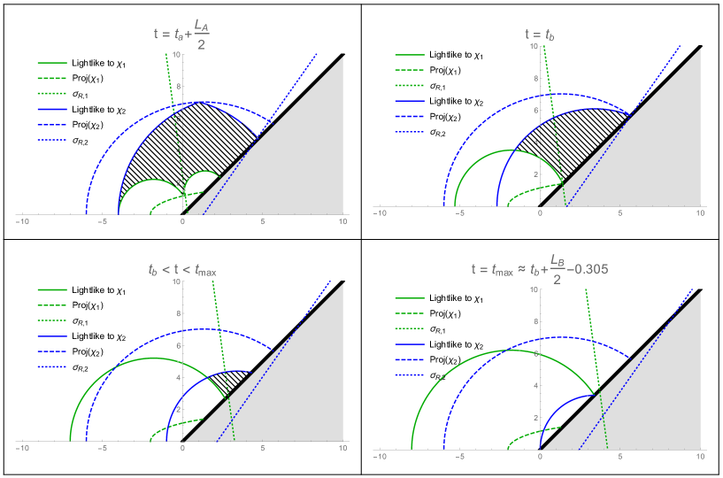
At a later time, (Figure 8, top left frame), we see the appearance of at the conformal boundary which represents the future tip of the causal diamond of on the conformal boundary where the blue and green lines intersect. Similar to , the curve will eventually terminate on the brane at some later time, which we will calculate explicitly.
At time (Figure 8, top right frame), we can see that the time slice intersects with closer to the brane indicated by the intersection of the green and blue lines, and the line-shaded region intersects with the brane along the brane interval .
As time progresses past into the regime where (Figure 8, bottom left frame), we will see that the line-shaded region will shrink and the intersection of the green and blue lines will become closer to the brane.
The last frame of Figure 8 occurs at which is the time where terminates on the brane and we have fully moved through the connected wedge through time. Naively, one might guess that the time scale should be given by . However, this is not the case. The reason for this can be clearly seen upon closer inspection of the final frame in Figure 8. Start by noting the intersection occurs to the left of both the dotted green and blue lines. This implies the point of intersection should be understood by projecting the null evolution of and in the region and respectively onto the brane. Referring to Appendix A.4 we can find expressions for these sheets in the appropriate regions given by . We need to find intersections of and . Using the fact that we can write
| (29) |
Setting will describe a curve. We know this curve has to terminate on the brane at the intersection point we are interested so restricting to the brane we can actually set which leads to a non-linear 2 by 2 system of equations.
| (30) |
We can find solutions to these equations and for our particular case we will numerically find
| (31) |
where and and and are explicitly given by Eq. (27). It is also possible to find solutions in closed form expressions but for the sake of simplicity of the presentation we just resort to numerically determining the time scale.
To conclude this section we will discuss the plot in Figure 9 which is the intersection of in the connected phase and with the brane for the same set of parameters considered in Figures 7 and 8.
The intersection of with the brane is contained in the intersection of the connected wedge with the brane. This will always be the case in our construction as long as EWN is satisfied. We compare the intersection of the connected wedge with the brane with the naive domain of dependence of denoted . We can see that the connected wedge is contained in . Generally, whenever EWN is respected, we will have .
As we have seen, the precise analytic understanding of the region is relatively complicated compared to understanding the entanglement wedges and . In the next set of Sections (Section 3) we will derive constraints in terms of the parameters which need to be satisfied to ensure that our entanglement wedges are well defined and satisfy EWN.
3 Entanglement Wedge Nesting in Poincaré AdS
In this section, we will study conditions on the relative location of constant time intervals and , which are located on the asymptotic boundary and on the cutoff brane respectively, such that EWN is satisfied, that is, . Clearly, this condition is only non-trivial if , ie., whenever we are in the connected phase. Assuming the latter, in Section 3.1 we derive a condition, presented in Eq. (43), on the time separation between and such that EWN holds. In Section 3.2 we study when the connected phase dominates and our conditions for EWN should be applied. We find that there are nontrivial configurations in which the RT surfaces are in the connected phase and EWN fails, although the intervals and are spacelike separated with respect to both the bulk and boundary metric. In Section 3.3, we argue that these violations appear whenever the RT surfaces in the connected or disconnected phase are not spacelike separated. In Section 3.4, we discuss how insisting that and be be spacelike separated in the bulk is generally not enough to ensure EWN will be satisfied. We connect this to the idea that the holographic theory on the cutoff surface is non-local which leads to a stronger requirement than spacelike separation of and to define independent subregions in non-local holographic theories. Finally, in Section 3.5, we compare our prescription for defining entanglement wedges/RT surfaces in cutoff holography with the restricted maximin prescription of Grado-White:2020wlb . Our results imply that while restricted maximin is designed such that EWN is satisfied under the condition that and are spacelike separated, the results obtained from restricted maximin disagree with a naive application of the RT formula if the “naive” RT surfaces corresponding to and are in causal contact. Even in the simplest cases, like the one we discuss, this can lead to RT surfaces which significantly differ from the naive expectation.
3.1 Condition for EWN
We will now derive conditions under which EWN holds. To this end consider two subregions and , located at constant times and , respectively. We choose to be a subset of the asymptotic boundary, while is a subset of the cutoff surface, i.e., the brane. Recall that EWN in our setup can only be violated when the connected phase dominates. Therefore, conditions that we derive in this section are only necessary and sufficient if the connected phase dominates. We will return to this point later in Section 3.2.
As a warm-up, let us begin with the special case of . In this situation the RT surfaces , , and which were defined in the previous section all lie on the same constant time slice. It is clear that since the partial Cauchy slices are contained in , the domain of dependence of is contained in the domain of dependence of ; in other words, . To see this, take any . Any causal curve going through must also go through . But since all causal curves passing through also intersect Thus, and must be a subset of . The proof for follows analogously.
Now, let us take the more general case in which . In this case, the strategy will be to ensure that the null congruences originating from or that enclose cannot puncture and . This means that causal signals originating from and, in particular, the complement of cannot influence events in and . As long as such a condition holds, we are guaranteed .
The condition that is unable to influence events in can be expressed as
| (32) |
where and are given in Eq. (12), and the index, , indicates whether we consider or . This condition arises from requiring that on every time-slice the spatial distance of the light congruence, which emanates from , to the center of the region is less than the distance of the curve to the center of region . As shown in Appendix B.1, it turns out that among the two conditions, the most stringent one is given by analyzing the constraint for , that is, the curve closer to the defect (c.f. Fig. 1). This condition can be rewritten as
| (33) |
The weaker condition we obtain from the analysis of takes the same form as Eq. (33) with the replacement . It is straightforward to see that Eq. (33) is not only a sufficient condition for EWN of in the connected phase, but also necessary, since violations of the condition necessarily lead to violations in EWN of because null congruences from will puncture .
Now we turn to the more complicated and involved case of deriving sufficient and necessary conditions to ensure . To obtain sufficient conditions for EWN we require that be spacelike separated from . However, following our discussion in Section 2.4.2 we know that we need to analyze the condition in a piecewise manner for each region , , and , defined with respect to the extremal surface . The condition that the points on which are spacelike separated from in or need to satisfy reads
| (34) |
where if the point lies in and if it lies in , while, as above, enumerates the two RT surfaces that connect and . This condition comes from requiring that and need to be spacelike separated to the entangling surface on the cutoff brane. For the points of that are located in , we impose the usual condition, familiar from the intervals at the asymptotic boundary, c.f., Eq. (32)
| (35) |
Out of the conditions written in Eqs. (34) and (35), we claim that it is sufficient for to satisfy Eq. (35) in . The reason for this is easily seen from Figure 10.
It depicts the various notions of spacelike separation to on some time slice . The collective conditions in Eq. (34) and Eq. (35) applied to the relevant regions can be visually understood as requiring to be outside the region enclosed by the solid red line. Moreover, satisfying only Eq. (35) in is equivalent to staying outside the region enclosed by the dashed green line. What is clear from Figure 10 is that a point being in the region outside the dashed green line implies that the same point is also outside the region enclosed by the solid red line. In Appendix B.1 we analyze the constraints in Eq. (35) for and show that it is satisfied inside whenever
| (36) |
where the right hand side defines the additional bounds .
Let us now investigate whether, under which circumstances, Eq. (36) is necessary. We begin by focusing on (that is, ). Suppose that we fix . As we vary or equivalently (cf., Eq. (12)) we will change the profile of the projection of onto a constant time slice without changing the endpoints. We know that since eventually intersects the boundary, a portion of always has to lie in . This just leaves us with the question of whether can lie in and . It is useful to note that if no portion of lies in then no portion of can lie within either. Therefore, showing that implies that . In Appendix B.2 we show that whenever , where is given by
| (37) |
To understand where this quantity comes from we define the point . When one can show that the tangent line to at will coincide with the ray in the -plane that separates the regions and . When , one can further show that the tangent line lives in . This implies that within some neighborhood of , . With some additional work detailed in Appendix B.2 we can prove that this is enough to show that throughout . An astute reader may notice that can actually become imaginary and worry about how our discussion will apply in such a scenario. We also cover such cases in Appendix B.2. Imaginary simply indicates that we have chosen a combination of such that for every choice of the tangent to at point will always lie in which means in such cases . So technically our condition should be iff . This implies that when is imaginary, satisfying the bound is not necessary to ensure EWN. This leaves us with the case where is real. To analyze this we define
| (38) |
Now consider the following expression,
| (39) |
It thus follows that and we have shown that . Using we can rewrite the condition as . Thus, whenever , it follows that . In other words, if the sufficient condition (36) is violated, we are in a regime where it is not necessary, since the extremal surface is completely contained in . Instead, the sufficient and necessary condition is simply the condition in Eq. (34) with . We show in Appendix B.1 that this is trivially satisfied when
| (40) |
which is equivalent to saying that and are spacelike separated.
A similar analysis can also be performed for , although with some differences. It is straightforward to convince oneself that there will always be portions of that live in and so it really only leaves us to understand under which conditions might live in . In Appendix B.2 we prove that iff either or and , where
| (41) |
is analogous to we defined in the analysis of with similar subtleties and interpretations we already discussed.111111The reader may be wondering why there are two distinct cases here. The reason for this is that unlike the ray that separates and , which always has a non-positive slope; the ray that separates and can have a positive or negative slope depending on the sign of . In the case where the ray has a negative slope and we can do a similar analysis as we did for by defining . In the case where the slope of the ray is non-negative and in such a case it is not possible for to be in . For the case of we can see that a violation of will necessarily lead to intersections of with null congruences originating from in arbitrarily small neighborhoods of . So in this case is necessary and sufficient. The remaining case of can be analyzed in an analogous manner as the case of . In fact, we can also show that which implies that anytime then which again will imply is both sufficient and necessary to ensure EWN in the connected phase.
Combining our results from the analysis of , we conclude that the necessary and sufficient condition to ensure in the connected phase is . We have to augment the two bounds with a minimum because the ordering between the two quantities changes depending on the specific choices of . Finally, we can formulate the condition for EWN of the entire setup (that is, ensuring that ) by requiring that . We can eliminate from the result by considering
| (42) |
It is easy to see that the right-hand side is positive from which it follows that . Since both and are positive, this implies that . This yields the final necessary and sufficient condition to ensure EWN of our setup in the event a connected phase dominates,
| (43) |
where and are defined in Eq. (33) and Eq. (36) respectively.
As a quick check it is useful to consider the limit as . In this limit the brane becomes a conformal boundary and we should recover standard holography results. Indeed, we can see that
| (44) |
Quick inspection of the expression in Eq. (42) reveals that . In other words, in the critical limit we recover standard holography results that EWN trivially follows from requiring spacelike separation of the intervals and .
3.2 Dominance of the Connected Phase
Thus far, we have been exploring the issue of when EWN is violated under the assumption that the RT surfaces associated to the region are in the connected phase, i.e., . This condition is necessary to have a non-trivial constraint from EWN. To finally show that EWN is violated, we need to discuss under which circumstances the condition
| (45) |
holds which implies that the RT surfaces are in the connected phase. Here, denotes the area of an extremal surface, while the subscript specifies which surface we are considering. In Appendix B.3 we analyze Eq. (45) and show that we can rephrase the condition of the RT surfaces being in the connected phase in terms of as with
| (46) |
where , , and . The condition for a connected phase places a lower bound on , which is intuitively clear since increasing the time between and makes the corresponding connected extremal surfaces more lightlike (i.e., decreases their area).
Recall that the condition for EWN, Eq. (43), places an upper bound on , while the condition for dominance of the connected phase places a lower bound on . Therefore, in order to have a genuine connected phase for which our EWN conditions are nontrivial, it is sufficient to check that the connected phase occurs before and become timelike separated, i.e., . This ensures that a connected phase dominates as from below. Using the fact that it is straightforward to see that generally, .121212This can be straightforwardly proved by noting that . Using this in Eq. (46) we can show that , which is clearly positive when . This implies that as a connected phase will always dominate.
It is also interesting to ask if a connected phase already exists as we approach from below. To facilitate our discussion, we will find it useful to understand when and when . Start by noting the following identity,
| (47) |
where we defined the length scale131313The positivity of can be seen as follows. Define and . Then . Then it is a straightforward exercise to explicitly compute and see .
| (48) |
It follows that, and . Using the length scale we numerically analyze the quantity . The details of our numerical analysis is discussed near the end of Appendix B.3 after Eq. (167). We find that whenever . Thus, if the subregion is sufficiently large, the connected phase will always dominate as we approach the EWN bound from below. This demonstrates that the constraint in Eq. (43) is non-trivial.
In the remaining regime where we find the opposite results, namely that (saturation occurs exactly when ). This implies that as the disconnected phase actually dominates. So it appears that for sufficiently small the condition for EWN we wrote only becomes relevant once and sufficiently close to . We organize all these results in Table 1.
| Disconnected | Connected | |
| Disconnected | Connected | |
| Connected | Connected |
In summary, we have shown that spacelike separateness of two regions and with respect to the bulk, is not sufficient to ensure EWN, at least if one of those regions is located at a finite cutoff in the bulk. When EWN precisely fails depends on the size of the involved intervals. At least in our case and for sufficiently large intervals we can give a precise condition, Eq. (43), which is equivalent to EWN. In the next section, we will demonstrate that the conditions we obtained for EWN can be reinterpreted as playing the role of ensuring that all extremal surfaces in our setup are spacelike separated from each other.
3.3 EWN and Spacelike Separation of Extremal Surfaces
To make more sense of the findings of Sections 3.1 and 3.2 it is useful to understand how the various extremal surfaces are separated from each other, in particular, whether they are spacelike separated. The conditions we derived for EWN in previous sections certainly guarantee that the line segments, and , generating the RT surface in the connected phase are always spacelike separated from the RT curves in the disconnected phase. However, we have not said anything about the separation between or or the separation between and , we will explore this in what follows.
Let us begin by investigating under which conditions the extremal surfaces and are spacelike separated. Start by noting that the congruence of null geodesics orthogonal to is simply given by
| (49) |
A point is spacelike separated from will satisfy Eq. (49) with the “” sign replaced by a “” sign. The RT surface is located at and , which is given in Eq. (11). Using this, we can write the condition for to be spacelike separated from as
| (50) |
This has to be true for any choice of . Since the right hand side of the inequality is a linear function of with a positive slope it means that the inequality is satisfied for if and only if it is satisfied at . Plugging this in we find
| (51) |
which, after isolating for , is precisely the condition that . This proves that is equivalent to requiring the spacelike separation of the disconnected RT surfaces. Importantly, this condition is actually stronger than simply requiring that and are spacelike separated in the bulk due to the computation we did in Eq. (42).
Now we turn to the issue of understanding when and are spacelike separated. We start by claiming that anytime then and cannot be spacelike separated. To prove this, it is useful to make use of the fact that we can can express as the intersection of lightcones located at the boundary whose apexes are located at the points given in Eq. (27).141414This statement is strictly speaking only true when . However, note that if we have that ¡1 when . For the purposes of our proof we need only show and fail to be spacelike separated from each other at and also very slightly above the bound as well so there is no issue here. Furthermore, the numerical calculations we did in Appendix B.4 make no such assumption and agree with what we have proved using this method. This means that is spacelike separated to (i.e. the extension of behind brane which we discussed near the end of Section 2.3) whenever151515Note the orientation of the inequality is correct. Since should be contained in the region enclosed by the lightcones whose apexes are at which makes timelike to .
| (52) |
Without loss of generality we will consider the case when . Let us consider the situation when and we set with ,
| (53) |
When we know that some subset of points on are in fact null separated from the point where . The next step is to determine which portion of is null separated from .161616The reason this step is necessary is because it is important to ensure that is null separated from (i.e. the point on needs to be null separated from some point on in front of the brane). This can be done by understanding where in the -plane the tip of the cone which defines what is spacelike separated from is equal to when . The answer is very simple; it is given by . The important aspect of this is . Now project our entire setup into the -plane and draw a straight line that goes from the tip of the cone located at to the point where intersects with the brane located at . It is straightforward to show that the slope of the straight line we constructed is negative for any choice of parameters in our setup. If we follow this ray it will intersect with at , where . It is precisely which is null separated from . So far we understand that at pair of points ( and ) the extremal surfaces become null separated when . Our next task is to understand what happens, we slightly perturb away from . To do this we consider the following,
| (54) |
When the expression above is also greater than zero. This represents a violation of the spacelike condition in Eq. (52) and implies that a portion of is now timelike separated from . Due to our previous discussion below Eq. (53) we can actually conclude that is timelike separated from as well as an open neighborhood of points on centered around . This proves our claim that cannot be spacelike to when .
Let us now turn to . In such a regime, there are a few comments that we can make based on the results of the computations in Eq. (53) and Eq. (54). In particular, we see that when in Eq. (53) the “” bound given in Eq. (52) is not violated. This suggests that, when only and fail to be spacelike separated from each other but all other points are indeed spacelike separated. The result in Eq. (54) in the case where suggests that the same pair of points are spacelike separated to each other when and indeed we should also expect all other points on and to be spacelike separated also as we reduce .171717Here, we only considered the “” bound of Eq. (52). We should also perform a similar analysis for “” bound, which however is harder to analyze. We thus resorted to numerical computations (see Appendix B.4) to verify that claims we made for . This is because if only a pair of points fail to be spacelike separated from at reducing to be below the marginal case increases the curves’ spacelike separation. Based on these observations, we expect that implies that and are spacelike separated. We have also verified this numerically in Appendix B.4.
We have thus shown that the necessary and sufficient condition for EWN we derived in Eq. (43) is equivalent to requiring that all the extremal surfaces we used to define our entanglement wedges (i.e. the surfaces , , ) are all spacelike separated from each other. In standard AdS this is guaranteed by spacelike separation of and in the bulk and boundary. However, as we have seen here, even in the simplest cases this is not true anymore in the presence of a cutoff.
Note that our construction of the entanglement wedge discussed in Section 2.4 only asked for points which were spacelike separated from and located between and . However, as seen above, the volume obtained this way is not necessarily the domain of dependence of a partial Cauchy slice . In the case of holography at a cutoff this enters as an additional requirement and in our case gives rise to the bound . All the different wedges we consider can only be constructed iff . The bound is logically independent of this and, as discussed below, ensures that the partial Cauchy slices and can lie on a single Cauchy slice.
3.4 Consequences for Locality in Cutoff Holography
From the analysis in Sections 3.1 – 3.3 we have learned that our condition for EWN, which was written in Eq. (43) non-trivially applies in the regime where . In this regime, the condition for EWN becomes which can be equivalently reinterpreted as the requirement that and are spacelike separated. This observation has implications for the discussion of non-locality in cutoff holography.
In standard holography the boundary theory is local and two subregions are independent if there are not causally related, i.e., they are spacelike separated. However, in cutoff holography one generally expects the theory on the cutoff to be a non-local theory and it is less clear how independent subregions can be defined. It has been known in our setup involving ETW branes that spacelike separation in the bulk sense is stronger than spacelike separation in the boundary sense Omiya:2021olc . An interesting open question in such setups is which notion of “spacelike” separation we need to define subregions on the holographic cutoff surface that are independent of each other. A naive candidate condition would be that the boundary subregions should be spacelike separated through the bulk as this ensures no causal signaling can occur between and either through the bulk or boundary.
Our computation in Eq. (42) proves that this requirement is not sufficient. In particular, as we have seen, it is possible to construct configurations in which and cannot influence each other causally through the bulk, but the entanglement wedges can. Such examples cannot be constructed in the case where (i.e. in standard holography). This implies that — provided entanglement wedges work in cutoff holography in the same way they do in standard AdS/CFT — and , and thus and , are not independent of each other even when and are spacelike separated through the bulk. We suggest that this should be regarded a geometric bulk manifestation of the non-local nature of the theory on the cutoff. In such cases our bound on entanglement wedge nesting disallows one to consider and as independent subregions. And clearly, the condition that cannot causally influence is a necessary condition for “independent” subregions in non-local holographic theories such as the one we have on the brane.
3.5 Relation to Restricted Maximin
Trying to define holography on a cutoff surface does not only cause problem for EWN, but also other inequalities which need to be obeyed by entanglement entropies, such as strong subadditivity (SSA). Based on ideas put forward in Wall:2012uf , the authors of Grado-White:2020wlb proposed a prescription, called restricted maximin, which associates a quantity which obeys SSA to any set of achronal co-dimension two bulk regions. This quantity is thus a natural candidate for a holographic entanglement entropy. It was further shown in Grado-White:2020wlb that their version of entanglement entropy also obeys monogamy of mutual information and the corresponding entanglement wedges satisfy EWN. It is interesting to contrast our construction of entanglement wedges to the construction using restricted maximin Grado-White:2020wlb .
In the restricted maximin prescription, one considers some subregion on the space-time boundary (which is allowed to be located at a finite cutoff) and then considers Cauchy surfaces in the bulk which end on the cutoff along a co-dimension 2 surface (i.e. ) such that . On each Cauchy slice one is instructed to find the minimal area surface homologous to . Maximizing the area of the minimal area surfaces over the choice of all Cauchy slices with the property yields the restricted maximin surface. In Grado-White:2020wlb it was shown that the construction of entanglement wedges using the maximin prescription satisfies EWN anytime the subregions on the cutoff/boundary are spacelike separated through the bulk. This is quite different from our conclusion which stated that simply requiring and to be spacelike separated is not sufficient to ensure EWN.
The key to resolving this apparent tension between our work and Grado-White:2020wlb is to note that our prescription for defining RT surfaces is generally not the same as in the restricted maximin approach. To understand this, recall that our approach starts with choosing the “naive” RT surfaces homologous to the subregions in which we are interested. What our results in Section 3.1-3.3 demonstrate is that such “naive” RT surfaces are generally not spacelike separated from each other. In our approach we need to enforce EWN non-trivially by restricting the placement of allowed boundary regions. This ensures that all the RT surfaces are spacelike separated. In the restricted maximin prescription, the construction always involves surfaces on restricted Cauchy slices, which ensures that all RT surfaces are already spacelike separated by construction. From this perspective, it is no surprise that EWN follows trivially from restricted maximin just by requiring and to be spacelike separated (i.e., EWN is “baked” into the maximin procedure through the ingredient of the restricted Cauchy slice). Furthermore, we expect that anytime EWN is respected in our prescription the “naive” and restricted maximin RT surfaces will coincide.
However, this also implies that there are configurations in which restricted maximin RT surfaces do not agree with the naive expectation. Consider the scenario used in this paper, where we have two spacelike separated subregions and at constant times and on a cutoff surface. As we have seen explicitly, it is possible to choose and such that and are spacelike separated, while their RT surfaces, which are located on constant time slices, are not. In particular, as demonstrated, this is possible for a static geometry. According to our prescription, such configurations should be ruled out, since EWN is violated. However, following restricted maximin it is indeed possible to assign an RT surface and an associated entropy. The price to pay is that even the disconnected, restricted maximin surfaces do not lie on constant time slices anymore, although the bulk geometry is static and both and are located on a constant time slice – in stark contrast to expectations from AdS/CFT. Although we do not intend to make definitive statements, a deviation between the “naive” and “restricted maximin” RT surfaces might indicate that the chosen boundary regions are not truly independent. This would in particular imply that partial traces over subregions have to be handled with care: Given subregions and which violate our EWN bounds one might want to compute the entanglement entropy of the reduced system on . However, when doing so using restricted maximin, one needs to remember to only consider Cauchy slices which are anchored on , although is not part of the system under consideration anymore.
We can summarize the relation between restricted maximin and our construction with the help of Figure 11, where we fix some values of and and plot the values of (solid green line), (solid blue line), (solid red line), and (dotted black line) as functions of .
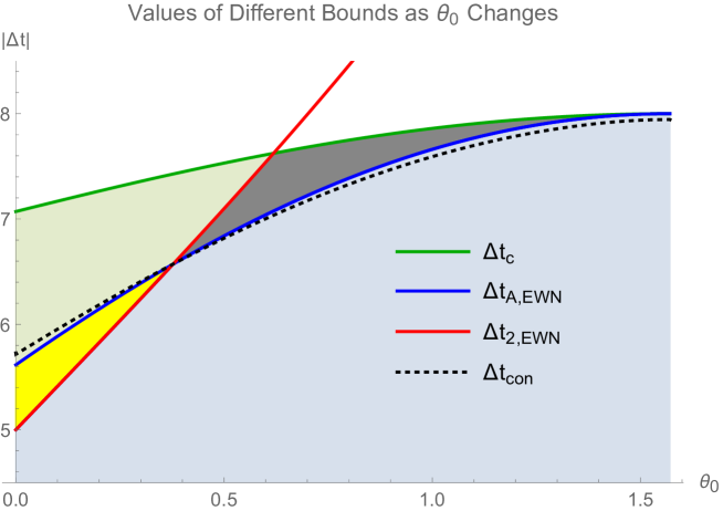
Start by noting that one can apply the restricted maximin procedure anywhere below the solid green line when and are spacelike separated, and one will always obtain entanglement wedges that satisfy the EWN (these wedges are defined using the maximin RT surfaces). In our prescription, we have learned that we can construct in the connected phase (as well as all other wedges) using the “naive” RT surfaces iff . This corresponds to the union of the gray and blue regions. The gray region is always below the red line but above the blue line and this implies are spacelike separated to each other but the disconnected RT surfaces , are not. In this portion of parameter space the disconnected RT surfaces in the restricted maximin prescription will not agree with our “naive” RT surfaces in the disconnected phase but we expect the connected RT surfaces to agree. The blue region () is where all “naive” RT surfaces are spacelike separated and EWN is satisfied. This is precisely the portion of parameter space where we expect all the maximin and “naive” RT surfaces to agree. This just leaves us with the union of the shaded green and yellow regions. In the yellow region, we are below the blue line but above the red line. Here we expect the disconnected phase maximin RT surfaces to match the “naive” ones but the connected ones will not match. Finally, in the green region we are above both the red and blue lines so none of the naive RT surfaces are spacelike separated from each other. In this parameter regime we expect no agreement between the maximin RT surfaces and the “naive” ones.
4 Entanglement Wedge Nesting in a Planar BTZ Black Hole Geometry
In this section, we will study conditions for entanglement wedge nesting for a two-sided planar BTZ black hole geometry with one exterior having an ETW brane by adapting the formalisms developed in the previous sections in AdS3. BTZ black hole geometry has also been of great interest in a variety of contexts ranging from black hole microstates Hartman:2013qma ; Kourkoulou:2017zaj ; Miyaji:2021ktr , brane world cosmologies Cooper:2018cmb ; Antonini:2019qkt ; Waddell:2022fbn , as well as constraining DGP couplings in brane-world setups Lee:2022efh , which motivates their study using our techniques.
In Section 4.1 we will introduce the two-sided BTZ black hole along with the ETW brane which will cut off a portion of the right exterior. We will also describe the configuration of intervals we will consider on the two exteriors. In particular, is an interval defined on the conformal boundary in the left exterior and is an interval defined on the right exterior on the brane. After doing this in Section 4.2 we derive expressions for the extremal surfaces we will be considering, which will be anchored to and . In 4.2.1 we give explicit expressions for thermal RT surfaces anchored to and which remain in their respective exteriors. In 4.2.2 we compute the connected RT surface which goes through the horizon and connects and . In Section 4.3 we give explicit expressions characterizing the wedges associated with the thermal RT surfaces depicted in Figures 13(a) - 13(b). In Section 4.4 we show that EWN of constrains the relative time shift between and in a way that prevents the RT surface in the connected phase from crossing the black hole “singularity”.
4.1 Two-Sided BTZ Black Holes with an ETW Brane
We start by discussing two-sided planar BTZ black hole with one side having an ETW brane. Nothing in what follows will depend on the fact that the black hole is planar, as long as the horizon size is sufficiently big relative to the brane and boundary intervals. The line element for the two sided BTZ black hole written in Kruskal-Szekeres coordinates is
| (55) |
where , , is the AdS radius, and is the horizon radius in Schwarzschild coordinates. The right and left conformal boundaries are located at and , respectively. In these coordinates, the future and past event horizons are located at . They split the spacetime into four distinct regions: The right and left exteriors,
| (56) | ||||
as well as the future and past interiors,
| (57) | ||||
see Figure 12.
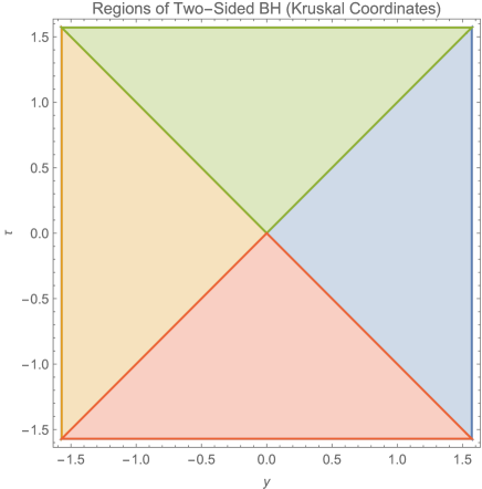
The Schwarzschild coordinate description of the exterior regions, , is related to the Kruskal coordinates through the change of coordinates
| (58) | ||||
Applying these coordinate transformations to the exterior region (), the line element given in Eq. (55) takes the form of the (planar) BTZ line element in Schwarzschild coordinates which covers the left (right) exterior region,
| (59) |
where , and . As we will see, using Schwarzschild coordinates is useful when discussing extremal surfaces which stay in the exterior regions, while Kruskal coordinates are beneficial to discuss extremal surfaces which start and end in the exterior regions, but cross through the interior regions. A particularly useful redefinition of the radial coordinate is so that the exterior exists for . Using this new radial coordinate gives the following expression for the planar BTZ black hole line element,
| (60) |
We now introduce an ETW brane in our setup. The ETW brane will be a timelike co-dimension one surface, which satisfies the following equations of motion involving the extrinsic curvature and induced metric
| (61) |
One can check that a hypersurface , satisfies the equation of motion above with
| (62) |
We will be interested in the case where the ETW brane is in the right exterior (i.e. ). With the help of the coordinate transformations in Eq. (58), we can also express the ETW brane in the right exterior in Schwarzschild coordinates as
| (63) |
We can see that in Schwarzschild coordinates the brane emerges from the past horizon at and falls into the future horizon at with some nontrivial profile in the plane in the right exterior.
4.2 Subregions and RT Surfaces
For the sake of mathematical simplicity we will restrict ourselves to a very limited configuration of boundary and brane intervals. In particular, we will consider constant Schwarzschild time slice intervals of equal length on both the boundary and brane centered at . We will only allow for a relative shift in time for the boundary and brane intervals. We will denote the the constant time interval on the left boundary at Schwarzschild time as . The constant time interval on the brane in the right exterior at Schwarzschild time will be denoted by . For the configuration of intervals on the asymptotic boundary and brane described above there are two kinds of possible RT surfaces which are discussed in the next two subsections.
4.2.1 Thermal Extremal Surfaces
Let us begin by finding extremal surfaces which stay within a single exterior region; we will call those thermal extremal surfaces. In the BTZ Due to time-translation symmetry in each region, thermal extremal surfaces are located on a constant Schwarzschild time-slice. We denote the thermal surface in left exterior anchored to the boundary as and the thermal surface in the right exterior anchored to the brane as . The extremal surfaces and are analogous to and in our previous AdS3 setup which will be used to construct disconnected wedges in our study of EWN. Thermal extremal surfaces extremize the area functional which in the BTZ geometry reads
| (64) |
with the horizon location in Schwarzschild coordinates (with radial coordinate ).
| (65) |
With some work, detailed in Appendix C.1, we obtain the following expression for a thermal RT surface anchored to a constant time slice () interval on the conformal boundary of (i.e. )
| (66) |
Using the expression above for the thermal RT surface anchored to a boundary interval we can also easily deduce the expression for the thermal RT surface which is anchored to a constant time slice interval on the brane at time in the right exterior (i.e. ). To do this we define the “virtual interval” associated to the interval on the brane denoted which is defined to be an interval which is obtained by continuing the RT surface anchored to the brane past the brane into the non-physical region. We can characterize this interval below,
| (67) |
The thermal RT surface is then described by
| (68) |
It it straightforward to see that , where is the part of the Planar BTZ spacetime not cut off by the brane (this just amounts to restricting the range of from to ). This gives the following, final, expression for , where
| (69) |
We can use our results to rewrite the same thermal RT surface in Kruskal coordinates using the inverse of the transformation Eq. (58). With a little bit of algebra and a careful distinction between the left and right exteriors the transformation from Schwarzschild to Kruskal coordinates reads
| (70) | ||||
where the different choice of signs give us the right and left exteriors. In particular, the left exterior is given when and the right exterior is given when . With some work detailed in Appendix C.1 we can express as
| (71) |
Similarly, is given by
| (72) |
4.2.2 Connected Extremal Surfaces
Connected extremal surfaces are extremal surfaces that connect the boundary and brane interval and pass through the interior of the black hole. We will denote them as .
To find the connected extremal surfaces we extremize the area function in Kruskal coordinates,
| (73) |
We can simplify the functional above by recalling that and are intervals with the same -coordinate for the endpoints. This means that a connected surface that starts at also needs to end at . This is only possible if . After setting we arrive at the task of extremizing the functional
| (74) |
With the work detailed in Appendix C.2, we arrive at the following general expression for the extremal curve(s) that go through the horizon and connects the brane and boundary intervals
| (75) |
For future convenience, we define . We can see that for a given a fixed value of (in the left exterior) the constant parameter will determine what (in the right exterior) will be and vice-versa. In the special case of the connected surface has a trivial horizontal profile in Kruskal time coordinates. As tends to the extremal curves become null.
When we do our analysis of entanglement wedge nesting we will find it useful to work in Schwarzschild coordinates. To find the expressions for the connected RT curves we start with Eq. (75) and make use of the coordinate transformation that takes exterior regions in Kruskal coordinates to Schwarzschild coordinates given by Eq. (58). The result is the following expression (see Appendix C.2 for details)
| (76) |
with constants given by
| (77) | ||||
The absolute value signs in the expressions are a book-keeping tool which circumvents the issue of worrying about the specific signs we need to use for for a given .
4.3 Construction of Entanglement Wedges
We now turn to discussing the entanglement wedges associated to the regions , , and . Starting with , we use to denote a partial Cauchy surface with boundary . We define the entanglement wedge of as the domain of dependence of . A convenient prescription which can be used to explicitly construct is by considering the a family of null geodesics beginning on which are also orthogonal to and evolve them towards the boundary. The set of these null geodesics enclose a co-dimension 0 region which is exactly as shown in Figure 13(a).
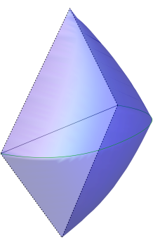
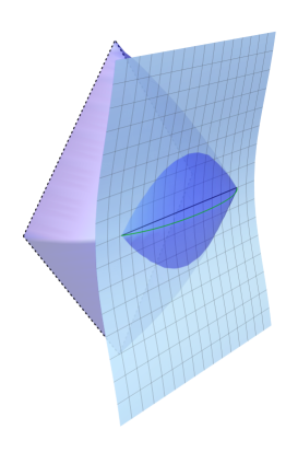
The points which belong to the entanglement wedge obey
| (78) |
where equality holds for the boundary of which is null (see Appendix C.4).
In an analogous manner we define the entanglement wedge associated with the region on the brane. We define as the partial Cauchy slice whose boundary is given by . Then the entanglement wedge of , denoted , is simply the domain of dependence of the . Furthermore, a more explicit construction of the of the wedge can be made by considering the a family of null orthogonal geodesics beginning on and evolve towards the boundary. The set of these null geodesics enclose a co-dimension 0 region which is exactly as shown in Figure 13(b).
As shown in Appendix C.4 the set of points in , satisfy
| (79) |
where we make the implicit restriction on to be in .
Finally, we turn to the definition of the entanglement wedge . As in the Poincare case, can be in one of two possible phases which we will call the connected and disconnected phase, depending on whether the RT surfaces connect the asymptotic boundary with the brane or not. In the disconnected phase we have which is simply the union of the separate entanglement wedges of and which we already discussed. In the connected phase we define as the partial Cauchy slice with a boundary given by . Then using this partial Cauchy slice we define the connected phase entanglement wedge as the domain of dependence of .
The explicit construction of in the connected phase can be done in a manner similar to what we outlined in Poincare AdS3, although the technical details will be different. Since for the purposes of finding constraints using EWN we only need to explicitly characterize the disconnected wedges, we refrain from explicitly characterizing the connected wedge here.
4.4 Conditions for EWN
In this section we will derive constraints on the parameters defining the separation of boundary and brane subregions in Kruskal time such that in the connected phase.
Just as in the Poincare AdS3 analysis in Section 3.1 a sufficient condition for EWN is given by requiring that all null geodesics originating from are unable to reach , i.e. no causal signals originating from can influence events in . Due to the trivial trajectory of the connected surface in the -plane, it suffices to ask when the points on the connected surface are spacelike separated from . The reason is that in our particular setup of brane and boundary intervals the connected surface always lies entirely the the region (depicted in Figure 20).
The points on the connected surface are spacelike (or possibly null) separated from points in if
| (80) |
where was defined in Eq. 79. Points that satisfy this inequality cannot influence events in , guaranteeing that . Substituting the location of the connected RT surface, Eg. (76) into Eq. (80) and rearranging the results as discussed in Appendix C.5 we obtain
| (81) |
Whenever this inequality is satisfied, EWN holds. It is possible to derive a specific constraint on the parameter which characterizes the connected surface. If we fix the parameters , , and and allow to vary (i.e. we fix the location and size of the brane interval and move the boundary interval up and down in time) then we can visualize the constraint with the help of the listed facts about the left hand side of (81) discussed in Appendix C.2, c.f. Figure 14.
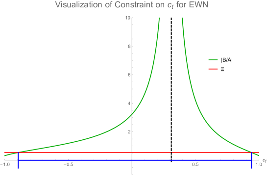
As we can see the right-hand side of the inequality in Eq. (81) is constant. The left-hand side explicitly depends on , has a vertical asymptote at and is non-zero and well defined everywhere else in the regime . Therefore, the inequality is only satisfied for some values with . The specific values of can be obtained by solving the equations
| (82) |
and solutions are181818Details of getting solution given in Appendix C.5.,
| (83) |
The tightest interval occurs when we take the limit of the expressions above as (i.e. when ) to give,
| (84) |
4.5 Constraints from EWN
Now that we have derived a sufficient condition for when EWN is respected in the connected phase we can continue and describe a nice geometric interpretation of what the tightest constraints given in Eq. (84) mean. First lets recall that a priori we just required that so the connected RT surfaces are spacelike. Now suppose we have a connected curve which starts on the left boundary at some Kruskal time . For the connected surface in Kruskal coordinates has a trivial horizontal profile and will end on the brane in the right exterior at the same Kruskal time as it started with at the boundary. However for more general values of less than unity one can imagine that there are certain values of where the surface would go through the past or future singularity before it hits the brane.
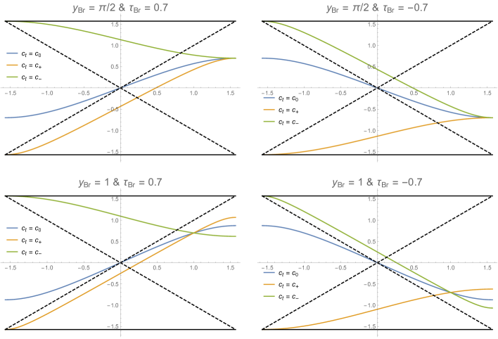
It turns out the the condition that EWN hold for intervals on the brane in the right exterior exactly excludes the configurations that would allow the connected surface to go through the singularity. In particular, if we fix the location of a constant time interval in the right exterior on the brane (i.e. fix and ) then the condition that EWN holds translates to
| (85) |
In Figure 15 we plot the connected surface in Kruskal coordinates in the -plane for , , and and see that the condition prevents the connected surface from going through the future and past singularities.
This is consistent with expectations from Lee:2022efh where the authors argued that connected RT surfaces that pass the “singularity” of a planar BTZ back hole cross, so that the orientation of the entanglement wedge flips. In practice, this means that the two connected components become timelike separated. Just like in Section 3, we can conclude that a violation of EWN comes from disconnected parts of the RT surface being able to causally influence each other.
5 Concluding Remarks
In this work, we have used basic examples to study the idea of associating an entanglement wedge for subregions located on cutoff surfaces and analyzed conditions for entanglement wedge nesting (EWN) to hold. More specifically, we focused on models where the cutoff surface takes the form of an end-of-the-world (ETW) brane in three dimensions, although our general prescription is independent of this. The prescription used to construct the entanglement wedge was to consider boundary and cutoff subregions, and , and naively apply the RT formula. Throughout the paper we chose and to be spacelike separated with respect to the bulk metric. Within this prescription, care has to be taken near the cutoff surface.
We demonstrated that even though the subregions and are spacelike separated, EWN can still fail. This is in contrast to standard AdS/CFT holography (which we recover from our results by sending the cutoff to the asymptotic boundary, i.e. in the AdS example and in the BTZ example) where spacelike separation of and implies EWN. Instead, to ensure EWN holds one needs stronger conditions, which we derived for two exemplary setups in Sections 3 and 4. The failure of EWN was caused in both cases by an unexpected timelike separation of RT surfaces. We would like to interpret this feature, where RT surfaces are not spacelike separated, even though the associated regions on the boundary or cutoff are, as a bulk manifestation of the non-local physics in the theory on the cutoff surface. It indicates that non-locality can make spacelike separated regions on the cutoff non-independent. We also related our construction to the restricted maximin procedure of Grado-White:2020wlb . We pointed out that while restricted maximin automatically satisfies EWN for spacelike separated subregions, it can give rise to RT surfaces with non-trivial profiles in time for constant time subregions in static geometries. We expect restricted maximin and our prescription agree when all RT surfaces are spacelike separated (or equivalently when EWN is respected).
Our understanding of holography at a finite cutoff is poor and we hope that a careful study of properties of entanglement wedges in the presence of a cutoff can shed light on the properties of holographic duals to finite subregions. It would in particular be interesting to generalize our results to more complicated geometries and interval configurations, also in higher dimensions. Optimistically, this could provide a set of rules which determine under which conditions cutoff and boundary subregions can be treated as truly independent. It is interesting to note that violations of the conditions we obtained for EWN throughout this paper have always started in arbitrarily small bulk neighborhoods of the entangling surface on the cutoff. Perhaps this will always be the case if a non-trivial violation of EWN occurs, such that it could be sufficient to focus on those regions which would significantly simplify the analyses. Even if this is not generally the case one might at least formulate some concrete necessary conditions for EWN to hold again, this may provide insight as to how one can naturally identify independent subregions on the boundary.
Another suggestive feature which warrants further investigation can be seen in Figure 9. This figure shows how the intersection of the entanglement wedge with the cutoff brane grows as we include further away regions (in this case on the asymptotic boundary). It is natural to interpret the intersection of the entanglement wedge with the cutoff surface as a domain of dependence, i.e., the spacetime subregion within which we can predict the state uniquely given a state on (or ). In a standard local quantum field theory, given a subsystem , we can predict the state within the naive domain of dependence of . Having access to a spacelike separated subregion does not affect this. For the theory on the cutoff, given we do not have access to the full naive domain of dependence. However, including far away regions increases the domain in which we can predict the state. Notably, as discussed, e.g., in Neuenfeld:2023svs , regions close to the boundary of the naive domain of dependence of correspond to UV information about the state on . This seems to indicate that for holographic cutoff theories IR information is stored locally, while UV information is stored non-locally in stark contrast to naive expectations. It would be very interesting to find a model which realizes such a behavior explicitly.
Acknowledgements.
I thank Niayesh Afshordi, Dominik Neuenfeld, Donald Marolf, Xi Dong, Samir Mathur, and Bin Guo for helpful discussions and comments as well as Dominik Neuenfeld for initial collaboration. The early stages of this work have also appeared in Krishan Saraswat’s Ph.D. thesis Saraswat:2023knb , which was supported by the University of Waterloo, Natural Sciences and Engineering Research Council of Canada (NSERC), and the Perimeter Institute for Theoretical Physics. Research at Perimeter Institute is supported in part by the Government of Canada through the Department of Innovation, Science and Economic Development Canada and by the Province of Ontario through the Ministry of Colleges and Universities. From August 2023 - 2024 this work was supported by Clifford Johnson, the University of Southern California, and the US Department of Energy for support under grant DE-SC 0011687.Appendix A Supplemental Calculations for Section 2
A.1 General Solution for Extremal Curves in Poincare AdS3
In this appendix we will find the general solution to the equations of motion that are obtain from the Lagrangian
| (86) |
which we read off from the function given in Eq. (8). Since there is no explicit dependence on there is a conserved Hamiltonian corresponding to -translations which can be written as
| (87) |
Furthermore, since there is no explicit time dependence we get the following equation for ,
| (88) |
Combining 87 and 88 we will obtain the following equations for and ,
| (89) |
where are constants. The general solution to the equations above is
| (90) |
which is what we wrote in Eq. (9). In the special case where the RT surface remains on a constant time slice and traces out a half circle in the bulk given by
| (91) |
It is straightforward to see that this is a half circle in the plane. It has a center at with a radius .
A.2 Spacelike Separated Points From Line Segments AdS3
Consider a spacelike line segment in AdS3 Poincare space parameterized in terms of
| (92) |
To understand the the set of points that are causally disconnected from the line segment we can consider an arbitrary point on the line segment , where . We consider the lightcone centered at the point
| (93) |
Next consider another point on the curve that is arbitrarily close to , with coordinates . The lightcone at that point is
| (94) |
Since is small we expand to obtain
| (95) |
We can find intersections of the light cones by solving
| (96) |
Setting the leading term to zero describes a plane of intersection after a small perturbation away from is made,
| (97) |
Note that the point is contained in the plane. Furthermore, we can express any tangent vector to the plane as follows,
| (98) |
with an appropriate choice of . Next consider the tangent vector to the curve at given by
| (99) |
Using these expressions we can explicitly show that , where . This demonstrates that the plane of intersection of cones near each other is along a plane that is orthogonal to the tangent vector along the curve with respect to the AdS3 inner product.
This fact is important to note because we can apply procedure for any point . It follows that we can generate the null surface which separates the spacelike and timelike regions in “most” of the bulk by shooting orthogonal geodesics from the curve. This prescription, however, is not the full story in fact we must also deal with the endpoints of the line segments. This is not difficult from our previous analysis we simply analyzed light cones to each point and the endpoints we will do a similar analysis. We start by noting the null surface we described by shooting null geodesics orthogonally is valid all the way up to . Recall that the set of orthogonal null geodesics will lie on the following orthogonal planes to the curve endpoints
| (100) |
These two planes will divide the spacetime into three regions:
-
•
are the set of points that are to the “left” of the orthogonal plane located at .
-
•
are the set of points that are to the “right” of the orthogonal plane located at
-
•
are the set of points that are enclosed by the planes and contain the line segment and is precisely where our procedure of finding spacelike points by emitting orthogonal null geodesics to the curve will be valid.
To find the set of spacelike separated points in regions it suffices to consider the light cones centered at the endpoints. This completes our formal discussion of how one can construct the null surfaces that allow one to determine what points are spacelike separated from a line segment.
To conclude this Appendix, lets apply this formalism to the RT curves in AdS3 with . Recall that we can write the extremal RT surface anchored to an interval with endpoints and as follows
| (101) |
The normal planes to the tangent at the conformal boundary at are given by
| (102) |
Generally one will find that this particular parametrization in terms of of the RT surface at the endpoints leads to a divergences for terms. This is not a problem with the formalism but rather a problem of the way we parameterized the surface. Lets instead parameterize the surface in terms of . We can write as
| (103) |
where the defines the two branches of the RT surface when when parameterize in terms of . We can plug this into to get
| (104) |
In this parametrization the equation of the plane normal to the tangent is given by
| (105) |
Once can explicitly check the derivatives are zero so the plane is given by
| (106) |
This shows that the RT curve ends on the conformal boundary orthogonally. This also implies that we can construct the null surface to which separates spacelike and timelike is generated by the geodesics shot orthogonal from the RT surface. In other words the entire AdS3 spacetime is so there is no need to worry about the light cones at the endpoints.
A.3 Extremal Curves with as Intersection of Light Cones
Lets go back to the line element of Poincare AdS3 it is given by:
| (107) |
We can see that under a Lorentz transformation of the form
| (108) |
gives
| (109) |
So extremal surfaces after Lorentz transforms remain extremal surfaces anchored to a boosted boundary interval. This allows us to simply take the extremal surface anchored to constant time slice boundary interval and boost the whole setup to get the extremal surface for a tilted interval. In particular, we could start with a constant time slice interval with endpoints and . The extremal surface is given by the following parametric equation in
| (110) |
One can check that the expression in Eq. (LABEL:ConstTimeSlicExtSSuf) is actually the intersection of the following two light cone surfaces
| (111) |
Next consider the case of a tilted interval on the boundary through a Lorentz boost with endpoints at and and . Since we were able to write the constant time slice extremal surface in terms of the intersection of two lightcones we should be able to write the new extremal surface in terms of the intersection of the lightcones with Lorentz transformed tips. In particular in the original coordinates we had a lightcone tip to the future of the extremal surface at and to the past of the extremal surface at . The future tip is Lorentz transformed to
| (112) |
The past tip is transformed to
| (113) |
Now we consider intersection of the two lightcones,
| (114) |
To find the intersection we solve,
| (115) |
With some simple algebra we find the intersection to be along the curve
| (116) |
where and . This indeed is the extremal surface we derived in Eq. (9) with the following identification of parameters
| (117) |
A.4 Expression for Null Evolution of for
Before writing the null evolution of it is useful to discuss some basic facts about identifying spacelike separated regions to extremal curves in AdS3 with .
Since every extremal curve with can be expressed as an intersection of certain bulk lightcones it is easy to find the set of spacelike separated regions to curves. Recall in Appendix A.3 we were able to show that the expression for the extremal surface written in Eq. (9) can be expressed as the intersection of the following lightcones
| (118) |
where and . We can express the intersection curve in terms of the coordinates of the cone tips as
| (119) |
where and . This allows us to express the set of spacelike separated points from the extremal curve towards the AdS3 boundary191919In Appendix A.2 we show that to understand the points that are spacelike separated to a line segment we can consider null surfaces generated by emitting null geodesics orthogonally from the RT curve. as
| (120) |
while the set of spacelike separated points away from the AdS3 boundary are given by
| (121) |
The lightcones given in Eq. (118) are generated by the family of null geodesics that are emitted orthogonally from the curve. These facts are useful when writing down expressions for the null sheets emitted from in .
Here we write the piecewise defined expression for the null sheets/congruence emitted from in the regime where , where .
| (122) |
where , , and . The signs appearing in Eq. (122) determine if the null points are have larger than (given by “” sign) or a smaller than (given by “” sign) , in the -plane for each fixed time slice. What we plot in the Figure 6 is at various fixed time slices 202020NOTE: The Heaviside step function, , used in Eq. (122) has a value of when the argument is zero (i.e. ).
Appendix B Supplemental Calculations for Section 3
B.1 Analysis of Conditions for EWN
In this Appendix we will analyze the conditions given in Eq. (32), Eq. (34), and Eq. (35) which will give us sufficient conditions for entanglement wedge nesting to hold.
We begin by considering the condition in Eq. (32), satisfying this condition ensures that no violations of EWN can occur for . For the condition reads
| (123) |
where and are given in Eq. (12). Along we have have the following relation between and ,
| (124) |
Substituting into the bound gives
| (125) |
So to satisfy the inequality throughout we must require
| (126) |
which is the result in Eq. (33) with .
Next we consider the conditions given in Eq. (35). For we we need to consider,
| (127) |
On the curve there is a relation between and given by,
| (128) |
We plug this into the inequality and simplify to obtain
| (129) |
So to satisfy the inequality throughout we require that
| (130) |
Which reproduces the bound we had in Eq. (36).
Finally, we will consider the condition in Eq. (34) with . For , we shall consider,
| (131) |
We claim that the inequality above is satisfied as long as . To demonstrate this we begin by noting that along we can express as , where and we also write . Then we have:
| (132) |
We can also express in terms of , , , and . Using Eq. (12) we can write,
| (133) |
Putting everything together we arrive at the following identity:
| (134) |
All we need to do now is demonstrate that the expression in the second line is negative. To do this, we note that the terms in the square brackets are non-negative and . Therefore it suffices to show that,
| (135) |
Expanding the left-hand side of the inequality above and rearranging the terms gives,
| (136) |
The set of of terms in in the second line are zero due to Eq. (133). We arrive at the following conclusion,
| (137) |
This proves that anytime the constraints in Eq. (34) with are satisfied.
B.2 Conditions when and
In this appendix we will be understanding when and . We will formulate the conditions by first fixing the spatial location of and (i.e. we fix ) and vary or equivalently and study what regions land in.
Lets begin by writing down the condition that needs to be satisfied to prove that for a certain placement of and we have that . To begin we must recall that the plane the separates the regions and is given by the expression written in Eq . (17). Since the profile along of the plane is trivial it suffices to simply refer to the plane as a ray in -plane and in this appendix this ray will be given by
| (138) |
The region to the immediate right of this ray is , therefore the condition that is equivalent to saying that is to the left of the ray . This can be formally written out as the following condition
| (139) |
where is given by Eq. (12). The strategy here will be to fix the parameters and vary (i.e. we vary and study if the inequality given in Eq. (138) is respected). As a first step we will analyze the inequality to linear order at the point where the brane intersects with . In this case we obtain
| (140) |
This places a constraint on of the form
| (141) |
So whenever this holds we will know that at least in a neighborhood of the point where the brane and intersect 212121The reader may be concerned that the expression for is not always going to be real. This is indeed true so the reader should really interpret the inequality is being true when . In the case when it is not real we can still show that ..
Now we will prove that this is not only true in a neighborhood of the point but for all . Start by noting that
| (142) |
This implies that if then we have that,
| (143) |
Now consider what happens when we set . We find that
| (144) |
This shows that when we have not just in small neighborhoods of but for all . Now consider any . Due to Eq. (143) we can write
| (145) |
This proves the statement that whenever then .
Now consider the case when becomes imaginary in this case we have that
| (146) |
We claim that when then for any value of . To prove this it suffices to show that
| (147) |
The reason for this is because of the the result we wrote in Eq. (143), it shows that . Therefore, satisfying the bounds written in Eq. (147) for is sufficient to have a bound for general values of . A simple computation reveals that
| (148) |
The quadratic term in is already positive and the linear term will also be positive whenever Eq. (146) is satisfied which is exactly when becomes imaginary. This proves our claim that whenever we know that .
Now lets turn to the task of deriving conditions for having . In this case the plane that separates and is given by the expression in Eq. (18). Just as before, the plane will have a trivial profile in and we will just refer to it as a ray in the -plane. Explicitly, the ray will be given by
| (149) |
To the right of this ray we will have the region so the condition to have is equivalent to saying that is to the left of the ray. This can be expressed as222222Notice that we actually have two different cases which did not appear when considering when . This was because the slope of the ray was always negative. However for the sign of the slope of the ray will depend on the sign of the quantity , hence we need to multiply the inequality in Eq. (LABEL:z2toLeftCondition) by the pre-factor of to account for the two cases.
| (150) |
where is given in Eq. (12 with ).
Lets begin by considering the case when (in this case the slope of the ray is negative). To linear order around we require
| (151) |
Using the linear order term we obtain the following condition on
| (152) |
This demonstrates that when (and also assuming that ) then in sufficiently small neighborhoods of the point where the brane intersects we have that . Using similar reasoning as we did in the study of when the condition that implies that throughout the whole domain given by . It is also straightforward to show that anytime 232323In particular we just go through analogous steps from Eqs.(143-147) with , , and . The expressions will take on similar forms and everything follows in a similar way as before..
This now leaves us with the case where (i.e. the ray separating and will have positive slope). In this case we can easily argue that . Start by noting that the region is described by . Consider the following quantity,
| (153) |
Lets analyze the quantity above in the domain . Since and it follows that when we know . Now lets consider the domain . Here it suffices to consider . Using this we can conclude that in the region . Combining everything we conclude that
| (154) |
Using the result above along with the fact that for all we can show
| (155) |
This proves that whenever then .
Finally, if then the ray separating and is a vertical line in the -plane (i.e. described by a line with ) in this case it is trivial to see that .
Lets now summarize the main results of this appendix:
-
•
if and only if:
-
–
242424Here we are combining the cases when is real or imaginary by simply putting bounds using the real part of . .
-
–
-
•
if and only if:
-
–
when .
-
–
Or if .
-
–
These results will be important towards finding the relevant necessary and sufficient constraints on such that EWN is respected in the connected phase in Section 3.1.
B.3 Condition for Dominance of Connected Phase
Below we will derive an inequality that determines when the connected phase will dominate. We start by writing expressions for , , and .
The regulated area for is
| (156) |
where , , and is given by Eq. (10). Performing the integral we obtain
| (157) |
The regulated area for is,
| (158) |
where is given by
| (159) |
and , , , , and is given by Eq. (12). Doing the integral and also a series expansion in we obtain
| (160) |
which gives the following the regulated length of ,
| (161) |
The area for is given by
| (162) |
where we use from Eq. (11) to obtain,
| (163) |
Note that here we did not use any regulator. This is because the distances between points on the brane away from the origin when are finite.
Using the expressions above we can write the condition in which the connected phase dominates as
| (164) |
which can be rewritten as follows
| (165) |
We can rearrange the inequality given in Eq. (165) and complete the square in to obtain
| (166) |
Using the facts that all the quantities are non-negative and also we can isolate for and arrive at
| (167) |
which is precisely what we mention in Eq. (46) with .
In Section 3.2, we discuss when the connected phase becomes dominant. In particular, we argued that the conditions we wrote for EWN would be non-trivial only if . This is because satisfying such a condition would imply that as the connected phase would dominate and our condition in Eq. (43) will need to be enforced in the connected phase. In particular, since , we should analyze and and determine their sign for various parameters. Since there are many parameters involved, we adopt the following approach in our analysis. First, we fix and . Then we plot or as a function of . This will give a single curve. Whenever the curve is above the -axis the connected phase will dominate, and when it is on or below the -axis the disconnected phase will dominate.
For example, in Figure 16 we plot both (left frame) and (right frame) as functions of for fixed and , and each colored line in the graph corresponds to a particular choice of 252525The reader might be wondering why we take the difference of squares rather than difference of the quantities themselves. It is just to reduce the number of square roots in our expression which can cause reduce numerical error when we get close to machine precision. We know the quantities themselves are always non-negative so can do this with. ut affecting our conclusions.. At first glance, we can see for certain choices of parameters the lines can be above or below the -axis. We can also see that when comparing between the left and right frames, lines of the same color (i.e. the lines that are plotted for same parameters and ) are above or below the -axis for the exact same interval(s) in . This can be seen visually in the plots, and verified through more precise numerical calculations. This is not just true for the particular sample we show but also more generally. This in fact is likely not a coincidence; it is a consequence of another fact that we numerically verified for many different choices of parameters. Which is, the roots of and are precisely given by solutions to , where we introduced in Eq. (48). In fact, recalling that by definition makes it very clear why the roots match for the same colored lines in Figure 16.
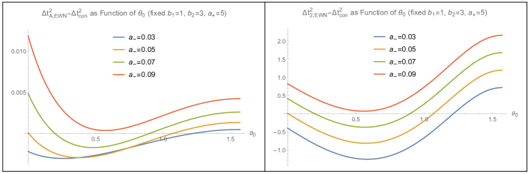
What all these numerical results suggest is that anytime we have 262626The implications occurs because we defined such that when . This implies that if we know then we also know . and anytime we have 272727The implications occurs because we defined such that when . This implies that if we know , then we also know .. We can verify this further through a more refined analysis by defining . When we fix to we will always have and when we will always be in the case where . In Figure 17 we make a Log plot (for , in left frame of Figure 17) and a Log plot (for , in right frame of Figure 17) as a function of .
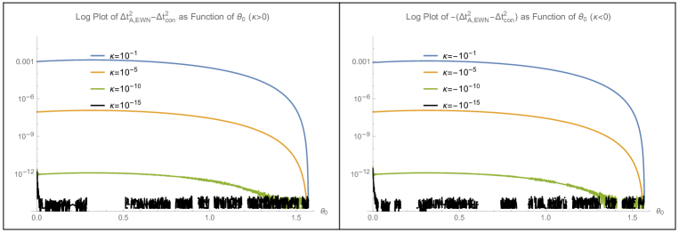
In the left frame we can see that when the value of and in the right frame we see when the value of . Furthermore, as , the value of as expected (one can check that similar results appear for more general choices of parameters as well, the wild oscillations we see in the curves as in the plots are artifacts of approaching machine precision).
Together, all these numerical results allow us to fill in the first two rows of Table 1, which tell us if the connected or disconnected phase dominates as .
B.4 Numerical Analysis of Spacelike Separation of
This Appendix discusses the details of our numerical analysis which further support the conjecture in Section 3.3 that and are spacelike separated. To explore the conjecture numerically we define a function of two variables
| (168) |
over the range of parameters where are defined in Eq. (12). We know that will be spacelike separated from iff . We analyze this numerically by first fixing the values of and , where and plotting the surface . Then we can determine if is spacelike to by simply checking if the surface is above the zero-plane. What we find in our numerical investigation is that in general whenever then remains above the zero plane and whenever a portion of dips below the zero plane. For example, in Figure 18 we plot as a blue surface and the zero plane as the orange surface with we have four frames for this choice of parameters with (top left frame), (top right frame), (bottom left frame), (bottom right frame).
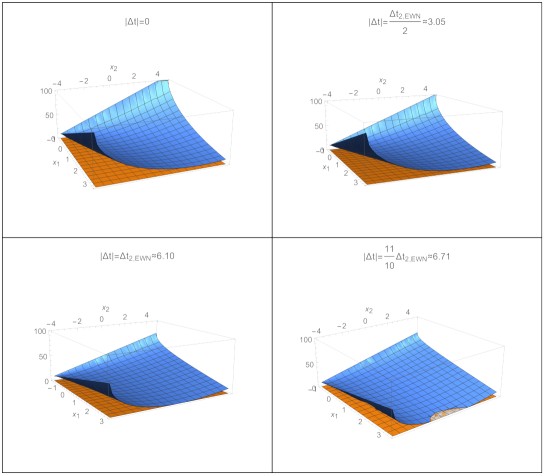
We can clearly see that when the blue surface stays above the zero plane, indicating that and are spacelike. We can also see that the shape of the blue plane is such that it gets closest to the zero plane along the slice. In Figure 19 we plot this particular slice in four frames with the same set of parameters as the frames in Figure 18.
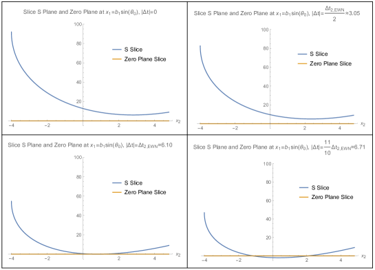
We can clearly see that when the blue plane will marginally touch the zero plane. In fact, the two bottom frames in Figure 19 are exactly the results we proved in Section 3.3 the two top frames of Figures 18 and 19 corroborate our claim that, indeed, and are spacelike separated. For more generic parameters, one can check that the results are similar.
Appendix C Supplemental Calculations for Section 4
C.1 Derivation of Thermal RT Surface
In this subsection we will derive the equations of motion to determine the thermal RT surface. We define the Lagrangian associated to the functional given in Eq. (64) as
| (169) |
Since the Lagrangian has no explicit dependence so we can define a conserved Hamiltonian associated with -translations given by
| (170) |
We have the following equation of motion for
| (171) |
where is constant. Plugging this into the Lagrangian we obtain the following expression for
| (172) |
Since we know that sign of the derivative will not change along the RT curve. Since we want to anchor the thermal RT surface to a constant time slice interval we must require that . This in turn means . If we plug this back into the equation for and rearrange for we get
| (173) |
We can see that when , this is the turning point for the RT curve where the derivative goes to zero. We want an RT surface that starts at extends into the bulk and then returns to the boundary at . Rearranging the expression we obtain the following integral equation for the “left portion” of the RT curve where
| (174) |
We can explicitly integrate each side of the expression and with some algebraic/trigonometric manipulations we arrive at
| (175) |
By requiring that we obtain the following relation between and
| (176) |
Plugging this back into the expression for gives
| (177) |
For the “right portion” of the RT curve we have to perform the following integrals
| (178) |
Based on our previous work on the left portion we can show the right portion of the RT curve will take the form
| (179) |
Once again, the requirement that gives
| (180) |
Using this we write
| (181) |
The condition that the two portions of the RT curves should be smoothly glued at and (i.e. ) gives the following equation
| (182) |
We can see that this requires the setting of as expected. So our final result for the thermal RT surface in Schwarzschild coordinates anchored to the endpoints of a constant time slice interval on the boundary centered around of size is
| (183) |
This gives the result we wrote in Eq. (66).
Schwarzschild to Kruskal Coordinates:
Now that we have derived the thermal RT surface in Schwarzschild coordinates we can use the expression given for the thermal RT surface along with the transformations given in in Eq. (70). Lets begin by computing the thermal surface in the left exterior which is anchored to an interval on the boundary at time . We have the following expressions for and
| (184) |
With these expressions we can write
| (185) |
This gives Eq. (71).
Next we proceed with writing the thermal RT surface anchored to a constant time slice interval on an ETW brane in the right exterior. We have the following expressions for and in the right exteriors
| (186) |
With similar manipulations as before we find that a thermal RT surface in the right exterior anchored to a constant time slice interval () centered around of length is given by
| (187) |
This gives the expressions in Eq. (72). We can check that the following identities hold,
| (188) |
which is exactly what we would expect from the coordinate transformations given in Eq. (58).
C.2 Derivation of Connected RT Surface
Derivation in Kruskal Coordinates:
We will go over the derivation of finding the connected RT surface that connects the brane and boundary intervals that are placed in the same position in the “-direction” (i.e. brane and boundary intervals have endpoints that are located at the same -coordinate location). The connected RT surface will consist of two line segments that go through the black hole horizon and connect the endpoints of the intervals on the brane and boundary which may exist on different time slices. To obtain such line segments we must extremize the functional given in Eq. (73). The Lagrangian associated to the functional is
| (189) |
Since there is no explicit -dependence we have
| (190) |
where is constant. Plugging in the actual Lagrangian gives the following expression for
| (191) |
We can see that within the bulk geometry a spacelike RT surface will have a derivative that is monotonic for . However, we also know that we must require the RT curve to start and end at the same -coordinate. This is only possible if . Therefore, we restrict ourselves to the set of RT surfaces with . This means we can deal with a much simpler Lagrangian
| (192) |
which is what we wrote in Eq. (74). Since we no longer have any explicit dependence on the Lagrangian we have another conserved quantity namely,
| (193) |
The extra factor is just a convenient normalization. Plugging in the appropriate Lagrangian gives
| (194) |
The sign of the above solution is determined by . In particular, when we have
| (195) |
The integrals can be done explicitly to obtain
| (196) |
Using the relation between and allows us to write
| (197) |
This gives us the expression for the connected RT surface in Eq. (75). Note that in general that . We can see for a fixed the value of fixes where in time the connected surface connects to the brane.
Connected Surface in Schwarzschild Coordinates:
Now that we have obtained an expression for the connected RT curve in Kruskal coordinates we can express it in the right exterior in Schwarzschild coordinates with the help of the coordinate transformations given in Eq. (58). Since we are interested analyzing entanglement wedge nesting in the right exterior in Schwarzschild coordinates. We will find it convenient to use the following expression for the connected surface in Kruskal coordinates
| (198) |
The connected RT surface ends on a brane located at where and at where . Recall the following relation between Kruskal and Schwarzschild coordinates
| (199) |
We can invert the relations above to obtain
| (200) |
where the “” is for the right exterior, the “” is for the left exterior. We focus on the right exterior and take the “” sign. From the equation of the connected surface we have
| (201) |
Now we plug in the expressions we had for and in Eq. (200) into Eq. (201) to obtain
| (202) |
Rearranging the expression above and recalling that , we obtain the following expression for the connected RT surface in the right exterior in Schwarzschild coordinates
| (203) |
An important point to note in the expression above is the issue of the sign of . In particular, depending on the precise value of the surface would extend away from the brane toward positive or negative . For example, if was fixed such that the connected surface moves toward larger then we certainly cannot have (at least in a arbitrarily small neighborhood of the brane). So the central question is how to understand if we should be in the case where or for a given . At first glance this may appear to be a rather complicated issue due to the expressions we wrote. However, there is a useful “trick” we can use to circumvent this problem.
To begin we do an expansion around the (near the brane) to get
| (204) |
One can check that the zeroth order term will evaluate to
| (205) |
This makes sense since should place us on the brane. Now lets focus on the linear order term. The linear order term will dictate if the brane is moving above or below the . In particular we want to to increase so the surface moves outward away from the brane this means the linear term should have an overall positive sign. This in turn means that we must require that . With the identity we showed for the zeroth order term we are able to write
| (206) |
Now we have a precise characterization of how the value of affects if or if . In particular, if and if . We can “automate/circumvent” these cases by strictly dealing with the following expression involving absolute values
| (207) |
This precisely gives us the expression for the connected surface in Schwarzschild coordinates in the right exterior given in Eq. (76).
For the sake of completeness, we can do a similar analysis and write down the connected surface in the left exterior as well. It is given by
| (208) |
Useful Properties of “”:
It is worthwhile to take the time to more carefully understand the properties of the ratio . We can explicitly write it as follows in terms of , , and
| (209) |
Since we want to strictly consider intervals on the brane in the right exterior we must require that we also note that . With this we conclude that: , , is singular at , and finally that is non-negative (i.e. monotonically increasing as increases) when . Using these facts we can easily deduce that when and when . So the sign of swaps at . One can easily check that the point of sign swapping occurs exactly when the connected extremal surface passes through the bifurcate horizon at . These facts will become important when we discuss conditions for entanglement wedge nesting.
C.3 Null Geodesics and Lightcones for Planar BTZ Background
In this appendix we will derive expressions the null geodesics propagating in the exterior spacetime of a planar BTZ black hole in Schwarzschild coordinates. The equations of motion for the geodesics will be obtained from the following Lagrangian (where we parameterize the geodesics trajectories using )
| (210) |
Using the fact that the the Lagrangian has no explicit or dependence we have the following conserved quantities
| (211) |
Dividing one equation by the other and squaring gives
| (212) |
where is some constant. Finally we can use the condition for having a null geodesic (i.e. ) to obtain the following first order equations that can be easily integrated,
| (213) |
In the special case where we choose a point on the boundary we can use the expressions above to obtain a fairly simple expression for a boundary lightcone
| (214) |
For more general cases the expression will be much more complicated and we will not explicitly write it here (nor will we require it in our discussions).
C.4 Entanglement Wedges For Constant Time Intervals in BTZ Background
An important fact about the thermal RT curves given in Eq. (66), which are anchored to constant time slice intervals on the boundary, is that they can be understood in terms of the intersection of certain lightcones whose apexes live on certain points on a conformal boundary (recall these lightcones are described by the equation given in Eq. (214)). In particular, for the thermal RT surface given in Eq. (66) we can define two lightcones. One lightcone is generated by past directed null geodesics originating from from the point given by,
| (215) |
The other lightcone consists of future oriented null geodesics originating from the point given by,
| (216) |
The surfaces will intersect along a curve on the constant time slice we can find this curve by setting
| (217) |
This is precisely the RT curve anchored to a constant time boundary interval. The region enclosed by and is called the causal wedge we can express the null boundary of the causal wedge in the following compact notation
| (218) |
where , which is what we wrote in Eq. (78). Points inside the causal wedge satisfy
| (219) |
Since the boundary of the causal wedge contains the set of points in the RT curve we can conclude a well-known fact that in the BTZ black hole background the causal and entanglement wedges are the same. We give an example of what it may look like in Figure 13(a).
For a constant time slice on the Brane in the BTZ background we take a similar approach to as we did for Poincare AdS3. For the interval on the brane we continue it past the brane and allow it to end on the boundary this defines a new constant time slice interval, the “virtual interval”, denoted which is defined as
| (220) |
Using this “virtual interval” we can construct its entanglement wedge in the full BTZ black hole background. Now we claim that the entanglement wedge associated to can be identified as . First we need to introduce the BTZ analogues of planes which will enable us to identify which we discussed in the AdS3 examples in Section 2.4.2. In the BTZ case the key is to appeal to the lightcones describing whose apexes are located at . The set of geodesics emitted from these apexes generates the null sheets that enclose . In particular, referring to our results in Appendix C.3 in Eq. (213) the set of null geodesics emitted from the apexes have the following profile in the -plane
| (221) |
The () branch are the set of null geodesics emitted toward (). These rays form a foliation of the spacetime in the -plane parametrized by . We can trivially extend these rays along the direction and define a foliation of the exterior BTZ geometry. The advantage of this foliation is that each individual null geodesic emitted from the apexes is restricted to a single leaf. The values for for the null geodesics that intersect the entangling surface on the brane is given by
| (222) |
This defines two planes in the BTZ background described by
| (223) |
As the subscripts suggest these are the BTZ analogues of the equations for we discussed in AdS3. Now it is straightforward to split the bulk into and we depict this in Figure 20 which (roughly speaking) is the BTZ analogue of Figure 10 obtained in the AdS3 analysis.
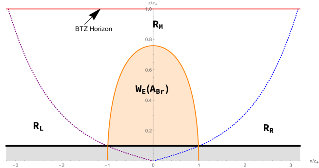
It should be stressed that Figure 20 should be properly understood as a the slice of the setup. When we go to a different slice the dotted lines which separate remain fixed, however, the solid black line representing the brane will shift away from to a different position given by Eq. (63). It will be more convenient to express the the trajectory of the brane in rather than coordinates. Using the transformation the trajectory of the brane reads
| (224) |
We will find it useful to express in terms of and . Using the fact that we will find that
| (225) |
Using this, we obtain the final form for the trajectory of the brane
| (226) |
where to reduce clutter we defined the horizon scaled variables , , , and . Taking the derivative of the brane trajectory with respect to one can easily see that it vanishes at and is positive(negative) for (). Consider some choice of the interval and lie on the time slice. We claim that any portion of the null congruence originating from behind the brane heading towards the boundary at will remain behind the brane at all times. By proving this we will be able to conclude that only null congruences from are needed to fully enclose a co-dimension one region (i.e. no need to amend with lightcones near the interval endpoints) and that .
Begin by writing down the trajectory of null geodesics that originate from and travel towards to boundary. These are given by the results in Eq. (213), using these, we can write the relevant trajectories in the -plane as
| (227) |
It is straightforward to see that when all the geodesics will intersect at the boundary at the apexes of the cones we described earlier and when the null geodesics will lie on . So we are interested in the time window . Each value of corresponds to a particular ray in the congruence emitted toward the boundary from . The rays which begin from behind the brane at are precisely the ones with where is given in Eq. (222) (note that these rays will live in and when the rays follow trajectories in the -plane corresponding to the dotted lines in Figure 20). We claim the family of rays we identified in the discussion above will always remain behind the brane. To prove this we compute
| (228) |
Analyzing the expression above we can clearly see that when we have that 282828Note that we need to make a restriction on since terminates on the boundary at whereas terminates later.. This means the trajectory of is bounded/nested in by . Next we consider the following computation
| (229) |
We can clearly see that anytime we have . This means the trajectory of is bounded/ nested in the trajectory of . In particular, all the rays that begin behind the brane with will be bounded by the rays with . So we need only show that rays with remains behind the brane when . This can be expressed mathematically as satisfying the bound
| (230) |
To prove the statement above we will make use of the fact that which was demonstrated through the calculation in Eq. (228). We can explicitly compute292929Note that the computation is made under the implicit assumption that with . This is sufficient because when we know that the brane advances towards larger when so there is no chance of rays starting behind the brane to end up in front. However, when the brane can move towards smaller values of which can pose a problem so we really only need to check the regime where . Furthermore, when the analysis will be similar in that case we only care about what will happen when .
| (231) |
By inspection of the expression above we can see that and saturation occurs only when . With this we can conclude that the condition in Eq. (230) is satisfied which proves the claim that rays emitted from towards the boundary which start behind the brane always remain behind the brane. This allows us to conclude that . We can explicitly write an inequality (which is in Eq. (79)) which characterizes the set of points in as
| (232) |
Where it is implicitly understood that we only keep points that are not cutoff by the ETW brane. In Figure 13(b) we given an example of what might look like.
C.5 Analysis of Condition for EWN
In this appendix we will manipulate the constraint given by Eq. (80) to obtain the inequality given in Eq. (81).
We begin by defining and then we rearrange the inequality in Eq. (80) to obtain
| (233) |
We have the following identity which comes from a trigonometric expansion
| (234) |
Using this we obtain
| (235) |
Next we plug in the explicit expression for from Eq. (76) and with some simple algebraic manipulations we arrive at
| (236) |
This gives us Eq. (81). It is useful to note that when we have
| (237) |
as long as , which it is. So we can see that EWN is always satisfied in our setup when .
We argued in Section 4.4 that to translate the constraint above to a constraint on simply requires us to find the appropriate solutions to,
| (238) |
The solutions to this equation will determine the endpoints on an interval in the parameter space over which EWN is satisfied. In particular, the parameter space over which EWN holds will take the form where and .
To get we solve
| (239) |
more explicitly the equation above reads,
| (240) |
and the relevant solution is given by
| (241) |
For we need to solve
| (242) |
which is the same equation as Eq. (240) with an added minus sign on the right-hand side. The relevant solution is given by
| (243) |
This gives us the bounds given in Eq. (83). It is not difficult to see from Figure 14 that to get the tightest bound we need to move the horizontal line representing the value of upwards. The highest it will go is when in that case we obtain the following results for ,
| (244) |
These are the bounds in Eq. (84).
C.6 Condition for Connected Phase
In this appendix we will go compute the areas of the connected and disconnected surfaces to determine when a connected phase will exist.
For the thermal RT surface anchored to the boundary we need to introduce a regulator/cutoff near the conformal boundary which we will send to zero when we analyze the condition for the connected phase. Specifically we will be interested in computing
| (245) |
One can easily compute the integral and show
| (246) |
For the thermal RT surface anchored to the brane there is no need for a regulator we can just do the computation directly. In this case we will be computing
| (247) |
Using the results from before we can immediately write
| (248) |
For the area of the connected surface we will find it convenient to compute the area in Kruskal coordinates. The area integral we will need to compute is given by
| (249) |
We can compute the anti-derivative of the integrand and obtain
| (250) |
We need to expand the result in terms of . To do this we need to note that the cutoff is defined in Schwarzschild coordinates. So using the expression for the connected surface given in Eq. (LABEL:LeftExteriorConnSch) we write
| (251) |
We can then express in terms of
| (252) |
Recall that sign of and should be the same so we actually can write the expressions without the absolute values and solve for and obtain (note that )
| (253) |
Now we use the coordinate transformation in Eq. (70) and obtain
| (254) |
This allows us to write
| (255) |
Now the condition for the connected phase will be
| (256) |
Plugging in all our expressions gives
| (257) |
In general we can see that as long as is sufficiently large, the inequality is satisfied, and therefore a connected phase is always guaranteed to exist as long as is sufficiently large. This makes the constraint we analyzed in the context of EWN relevant in the limit where (i.e. the constraint we wrote in Eq. (84)).
References
- (1) B. Grado-White, D. Marolf and S. J. Weinberg, Radial Cutoffs and Holographic Entanglement, JHEP 01 (2021) 009 [2008.07022].
- (2) J. M. Maldacena, The Large N limit of superconformal field theories and supergravity, Adv. Theor. Math. Phys. 2 (1998) 231 [hep-th/9711200].
- (3) E. Witten, Anti-de Sitter space and holography, Adv. Theor. Math. Phys. 2 (1998) 253 [hep-th/9802150].
- (4) S. S. Gubser, AdS / CFT and gravity, Phys. Rev. D 63 (2001) 084017 [hep-th/9912001].
- (5) H. Nastase, Introduction to AdS-CFT, 0712.0689.
- (6) J. Polchinski, Introduction to Gauge/Gravity Duality, in Theoretical Advanced Study Institute in Elementary Particle Physics: String theory and its Applications: From meV to the Planck Scale, pp. 3–46, 10, 2010, 1010.6134, DOI.
- (7) M. Ammon and J. Erdmenger, Gauge/gravity duality: Foundations and applications. Cambridge University Press, Cambridge, 4, 2015, 10.1017/CBO9780511846373.
- (8) M. Van Raamsdonk, Lectures on gravity and entanglement., in Theoretical Advanced Study Institute in Elementary Particle Physics: New Frontiers in Fields and Strings, pp. 297–351, 2017, 1609.00026, DOI.
- (9) S. S. Gubser, I. R. Klebanov and A. M. Polyakov, Gauge theory correlators from noncritical string theory, Phys. Lett. B 428 (1998) 105 [hep-th/9802109].
- (10) S. de Haro, S. N. Solodukhin and K. Skenderis, Holographic reconstruction of space-time and renormalization in the AdS / CFT correspondence, Commun. Math. Phys. 217 (2001) 595 [hep-th/0002230].
- (11) S. Cooper, M. Rozali, B. Swingle, M. Van Raamsdonk, C. Waddell and D. Wakeham, Black hole microstate cosmology, JHEP 07 (2019) 065 [1810.10601].
- (12) M. Miyaji and T. Takayanagi, Surface/State Correspondence as a Generalized Holography, PTEP 2015 (2015) 073B03 [1503.03542].
- (13) M. Miyaji, T. Numasawa, N. Shiba, T. Takayanagi and K. Watanabe, Continuous Multiscale Entanglement Renormalization Ansatz as Holographic Surface-State Correspondence, Phys. Rev. Lett. 115 (2015) 171602 [1506.01353].
- (14) A. B. Zamolodchikov, Expectation value of composite field T anti-T in two-dimensional quantum field theory, hep-th/0401146.
- (15) Y. Jiang, Lectures on solvable irrelevant deformations of 2d quantum field theory, 2019, https://api.semanticscholar.org/CorpusID:140264614.
- (16) G. Bonelli, N. Doroud and M. Zhu, -deformations in closed form, JHEP 06 (2018) 149 [1804.10967].
- (17) S. Dubovsky, V. Gorbenko and M. Mirbabayi, Asymptotic fragility, near AdS2 holography and , JHEP 09 (2017) 136 [1706.06604].
- (18) S. Grieninger, Entanglement entropy and deformations beyond antipodal points from holography, JHEP 11 (2019) 171 [1908.10372].
- (19) D. J. Gross, J. Kruthoff, A. Rolph and E. Shaghoulian, in AdS2 and Quantum Mechanics, Phys. Rev. D 101 (2020) 026011 [1907.04873].
- (20) A. Cavaglià, S. Negro, I. M. Szécsényi and R. Tateo, -deformed 2D Quantum Field Theories, JHEP 10 (2016) 112 [1608.05534].
- (21) L. McGough, M. Mezei and H. Verlinde, Moving the CFT into the bulk with , JHEP 04 (2018) 010 [1611.03470].
- (22) M. Guica and R. Monten, and the mirage of a bulk cutoff, SciPost Phys. 10 (2021) 024 [1906.11251].
- (23) A. Lewkowycz, J. Liu, E. Silverstein and G. Torroba, and EE, with implications for (A)dS subregion encodings, JHEP 04 (2020) 152 [1909.13808].
- (24) T. Takayanagi, Holographic Dual of BCFT, Phys. Rev. Lett. 107 (2011) 101602 [1105.5165].
- (25) A. Almheiri, R. Mahajan, J. Maldacena and Y. Zhao, The Page curve of Hawking radiation from semiclassical geometry, JHEP 03 (2020) 149 [1908.10996].
- (26) H. Z. Chen, R. C. Myers, D. Neuenfeld, I. A. Reyes and J. Sandor, Quantum Extremal Islands Made Easy, Part I: Entanglement on the Brane, JHEP 10 (2020) 166 [2006.04851].
- (27) H. Z. Chen, R. C. Myers, D. Neuenfeld, I. A. Reyes and J. Sandor, Quantum Extremal Islands Made Easy, Part II: Black Holes on the Brane, JHEP 12 (2020) 025 [2010.00018].
- (28) J. Hernandez, R. C. Myers and S.-M. Ruan, Quantum extremal islands made easy. Part III. Complexity on the brane, JHEP 02 (2021) 173 [2010.16398].
- (29) G. Grimaldi, J. Hernandez and R. C. Myers, Quantum extremal islands made easy. Part IV. Massive black holes on the brane, JHEP 03 (2022) 136 [2202.00679].
- (30) D. Neuenfeld, Double holography as a model for black hole complementarity, 2021, https://api.semanticscholar.org/CorpusID:233714953.
- (31) D. Neuenfeld, The Dictionary for Double Holography and Graviton Masses in d Dimensions, 2104.02801.
- (32) H. Omiya and Z. Wei, Causal structures and nonlocality in double holography, JHEP 07 (2022) 128 [2107.01219].
- (33) H. Geng, A. Karch, C. Perez-Pardavila, L. Randall, M. Riojas, S. Shashi et al., Constraining braneworlds with entanglement entropy, SciPost Phys. 15 (2023) 199 [2306.15672].
- (34) N. Engelhardt and A. C. Wall, Quantum Extremal Surfaces: Holographic Entanglement Entropy beyond the Classical Regime, JHEP 01 (2015) 073 [1408.3203].
- (35) S. Ryu and T. Takayanagi, Holographic derivation of entanglement entropy from AdS/CFT, Phys. Rev. Lett. 96 (2006) 181602 [hep-th/0603001].
- (36) V. E. Hubeny, M. Rangamani and T. Takayanagi, A Covariant holographic entanglement entropy proposal, JHEP 07 (2007) 062 [0705.0016].
- (37) W. Donnelly and V. Shyam, Entanglement entropy and deformation, Phys. Rev. Lett. 121 (2018) 131602 [1806.07444].
- (38) M. Headrick and T. Takayanagi, A Holographic proof of the strong subadditivity of entanglement entropy, Phys. Rev. D 76 (2007) 106013 [0704.3719].
- (39) A. C. Wall, Maximin Surfaces, and the Strong Subadditivity of the Covariant Holographic Entanglement Entropy, Class. Quant. Grav. 31 (2014) 225007 [1211.3494].
- (40) M. Headrick, V. E. Hubeny, A. Lawrence and M. Rangamani, Causality & holographic entanglement entropy, JHEP 12 (2014) 162 [1408.6300].
- (41) C. Akers, J. Koeller, S. Leichenauer and A. Levine, Geometric Constraints from Subregion Duality Beyond the Classical Regime, 1610.08968.
- (42) C. Akers, V. Chandrasekaran, S. Leichenauer, A. Levine and A. Shahbazi Moghaddam, Quantum null energy condition, entanglement wedge nesting, and quantum focusing, Phys. Rev. D 101 (2020) 025011 [1706.04183].
- (43) B. Chen, B. Czech and Z.-z. Wang, Quantum information in holographic duality, Rept. Prog. Phys. 85 (2022) 046001 [2108.09188].
- (44) S. Leutheusser and H. Liu, Subregion-subalgebra duality: emergence of space and time in holography, 2212.13266.
- (45) A. Karch and L. Randall, Locally localized gravity, JHEP 05 (2001) 008 [hep-th/0011156].
- (46) R. Bousso and G. Penington, Entanglement wedges for gravitating regions, Phys. Rev. D 107 (2023) 086002 [2208.04993].
- (47) H. Geng, Some Information Theoretic Aspects of De-Sitter Holography, JHEP 02 (2020) 005 [1911.02644].
- (48) D. Neuenfeld and M. Srivastava, On the causality paradox and the Karch-Randall braneworld as an EFT, JHEP 10 (2023) 164 [2307.10392].
- (49) J. H. Lee, D. Neuenfeld and A. Shukla, Bounds on gravitational brane couplings and tomography in AdS3 black hole microstates, JHEP 10 (2022) 139 [2206.06511].
- (50) H. Geng and A. Karch, Massive islands, JHEP 09 (2020) 121 [2006.02438].
- (51) K. Doi, J. Harper, A. Mollabashi, T. Takayanagi and Y. Taki, Pseudoentropy in dS/CFT and Timelike Entanglement Entropy, Phys. Rev. Lett. 130 (2023) 031601 [2210.09457].
- (52) B. Liu, H. Chen and B. Lian, Entanglement entropy of free fermions in timelike slices, Phys. Rev. B 110 (2024) 144306 [2210.03134].
- (53) K. Doi, J. Harper, A. Mollabashi, T. Takayanagi and Y. Taki, Timelike entanglement entropy, JHEP 05 (2023) 052 [2302.11695].
- (54) Z. Li, Z.-Q. Xiao and R.-Q. Yang, On holographic time-like entanglement entropy, JHEP 04 (2023) 004 [2211.14883].
- (55) T. Hartman and J. Maldacena, Time Evolution of Entanglement Entropy from Black Hole Interiors, JHEP 05 (2013) 014 [1303.1080].
- (56) I. Kourkoulou and J. Maldacena, Pure states in the SYK model and nearly- gravity, 1707.02325.
- (57) M. Miyaji, T. Takayanagi and T. Ugajin, Spectrum of End of the World Branes in Holographic BCFTs, JHEP 06 (2021) 023 [2103.06893].
- (58) S. Antonini and B. Swingle, Cosmology at the end of the world, Nature Phys. 16 (2020) 881 [1907.06667].
- (59) C. Waddell, Bottom-up holographic models for cosmology, JHEP 09 (2022) 176 [2203.03096].
- (60) K. Saraswat, Quantum Aspects of Black Holes: From Microstates to Echoes and Somewhere In-Between, Ph.D. thesis, U. Waterloo (main), 2023.