Convergence Analysis of the Wasserstein Proximal Algorithm beyond Geodesic Convexity

Abstract

The proximal algorithm is a powerful tool to minimize nonlinear and nonsmooth functionals in a general metric space. Motivated by the recent progress in studying the training dynamics of the noisy gradient descent algorithm on two-layer neural networks in the mean-field regime, we provide in this paper a simple and self-contained analysis for the convergence of the general-purpose Wasserstein proximal algorithm without assuming geodesic convexity of the objective functional. Under a natural Wasserstein analog of the Euclidean Polyak-Łojasiewicz inequality, we establish that the proximal algorithm achieves an unbiased and linear convergence rate. Our convergence rate improves upon existing rates of the proximal algorithm for solving Wasserstein gradient flows under strong geodesic convexity. We also extend our analysis to the inexact proximal algorithm for geodesically semiconvex objectives. In our numerical experiments, proximal training demonstrates a faster convergence rate than the noisy gradient descent algorithm on mean-field neural networks.

1 Introduction

Minimizing a cost functional over the space of probability distributions has recently drawn widespread statistical and machine learning applications such as variational inference [23, 14, 37], sampling [31, 30, 5], and generative modeling [34, 7], among many others. In this work, we consider the following general optimization problem:

$$\min_{\rho\in\mathcal{P}_{2}({\Theta})}F(\rho),$$ (1)

where $F$ is a real-valued target functional defined on the space of probability distributions $\mathcal{P}_{2}({\Theta})$ with finite second moments on $\Theta\subset\mathbb{R}^{d}$. Our motivation for studying this problem stems from analyzing training dynamics of the Gaussian noisy gradient descent algorithm on infinitely wide neural networks, which can be viewed as a forward time-discretization of the mean-field Langevin dynamics (MFLD) [26, 15]. Given the connection between sampling and optimization, the continuous-time MFLD is an important example of the Wasserstein gradient flow corresponding to minimizing an entropy-regularized total objective function of large interacting particle systems (cf. Section 2.1).

On the other hand, the Wasserstein gradient flow is conventionally constructed by the following proximal algorithm,

$$\rho_{n+1}=prox_{F,\xi}(\rho_{n}):=\operatorname*{arg\,min}_{\tilde{\rho}\in\mathcal{P}_{2}({\Theta})}\left\{F(\tilde{\rho})+\dfrac{1}{2\xi}\mathcal{W}_{2}^{2}(\tilde{\rho},\rho_{n})\right\},$$ (2)

where $\xi>0$ is the time-discretization step size. The Wasserstein proximal algorithm (2) is an iterative backward time-discretization procedure for solving (1) and it is also known as the JKO scheme introduced in a seminal work [16]. In contrast to various forward-discretization methods such as gradient descent over $\mathcal{P}_{2}({\Theta})$ and the Langevin sampling algorithms [10, 30, 5], proximal algorithms are often unbiased in the sense that their convergence guarantees do not depend on the dimension-dependent discretization error with positive step size and they are often more stable than the forward gradient descent algorithms without strong smoothness condition [37, 36, 29, 7]. While the proximal algorithms for geodesically convex functionals are well studied in the literature, it remains an open question whether they can maintain similar unbiased and linear convergence guarantees in discrete time beyond the geodesic convexity. Current work fills this important gap by establishing linear convergence results without assuming geodesic convexity on the objective functional $F$.

Our general quantitative convergence rate for the Wasserstein proximal algorithm offers an alternative training scheme to the noisy gradient descent for two-layer neural networks in the mean-field regime. Specifically, a two-layer neural network is parameterized as

$$f(x;{\bm{\theta}}):=\dfrac{1}{m}\sum_{j=1}^{m}\varphi(\theta_{j};x)=\int_{\Theta}\varphi(\theta;x)d\rho^{m}(\theta),$$ (3)

where ${\bm{\theta}}=(\theta_{1},\theta_{2},...,\theta_{m})\in\mathbb{R}^{d\times m}$ and $\rho^{m}=\frac{1}{m}\sum_{j=1}^{m}\delta_{\theta_{j}}$ is the empirical distribution of the hidden neuron parameters. The perceptron $\varphi(\theta_{j};x)$ in (3) can take the form $\varphi(\theta_{j};x)=\sigma(\theta_{j}^{\top}x)$ where $\sigma$ is some nonlinear activation function. Given a training dataset $(x_{i},y_{i})_{i=1}^{N}\sim p(x,y)$ and a convex loss function $l(\cdot)$ (such as the squared loss and logistic loss), the $L^{2}$-regularized training risk is defined as

$$\begin{gathered}R({\rho^{m}})={1\over N}\sum_{i=1}^{N}l(f(x_{i};{\bm{\theta}}),y_{i})+\dfrac{\lambda}{m}\sum_{j=1}^{m}\left\|\theta_{j}\right\|^{2}\\ \qquad\qquad\qquad\qquad={1\over N}\sum_{i=1}^{N}l\left(\int_{\Theta}\varphi(\theta;x_{i})d\rho^{m}(\theta),y_{i}\right)+\lambda\int_{\Theta}\left\|\theta\right\|^{2}d\rho^{m}(\theta).\end{gathered}$$ (4)

where $\lambda>0$ is the coefficient of $L_{2}$-regularization. The Gaussian noisy gradient descent algorithm on the $L^{2}$-regularized training risk can be written as the following stochastic recursion

$$\theta^{n+1}_{j}=\theta^{n}_{j}-\xi\nabla{\delta R\over\delta\rho}(\frac{1}{m}\sum_{\ell=1}^{m}\delta_{\theta_{\ell}^{n}})(\theta^{n}_{j})+\sqrt{2\xi\tau}z_{nj},$$ (5)

where $z_{nj}$ are i.i.d. $\mathcal{N}(0,I)$ and $\tau>0$ represents the Gaussian noise variance. In (5), ${\delta R\over\delta\rho}(\rho)$ is the first variation of $R$ at $\rho$ (cf. Definition A.2). The limiting dynamics of (5) under $m\rightarrow\infty$ and $\xi\rightarrow 0$ is called the continuous-time MFLD [15]. Under a uniform log-Sobolev inequality (LSI) assumption (cf. Definition C.1), linear convergence of MFLD to the optimal value of the total objective ($L^{2}$-training risk plus an entropy term) is established in [27, 6], and the noisy gradient descent algorithm is subject to a dimension-dependent time-discretization error [27], which may slow down the convergence.

To remove the time-discretization error, we may instead train the neural network with the Wasserstein proximal algorithm (2). Since such neural network architecture satisfies the uniform LSI which in turn implies a Wasserstein Polyak-Łojasiewicz (PL) inequality (cf. Definition 3.2), our algorithm can achieve an unbiased linear rate of convergence to a global minimum of total objective.

1.1 Contributions

In this work, we give a simple and self-contained convergence rate analysis of the Wasserstein proximal algorithm (2) for minimizing the objective function satisfying a PL-type inequality without resorting to any geodesic convexity assumption. Below we summarize our main contributions.

• To the best of our knowledge, current work is among the first works to obtain an unbiased and linear convergence rate of the general-purpose Wasserstein proximal algorithm for optimizing a functional under merely a PL-type inequality. When restricted to $\mu$-convex ($\mu>0$) objective functional, our result yields a sharper linear convergence rate (in function value and minimizer under $\mathcal{W}_{2}$ distance) than the existing literature [37, 7].

• The linear convergence guarantee provides a new training scheme for two-layer wide neural networks in the mean-field regime. Our numeric experiments show a faster training phase (up to particle discretization error) than the (forward) noisy gradient descent method.

• We also analyze the inexact proximal algorithm for geodesically semiconvex objectives under PL-type inequality.

1.2 Literature review

Recently, various time-discretization methods have been proposed for minimizing a functional over a single distribution. Different from the proximal algorithm, some explicit forward schemes that can be seen as gradient descent in Wasserstein space are proposed [8, 24]. For example, [8] studies a gradient descent algorithm for solving the barycenter problem on the Bures-Wasserstein manifold of Gaussian distributions. The Langevin algorithm, as another forward discretization of Wasserstein gradient flows via its stochastic differential equation (SDE) recursion, is widely used in the sampling literature. Numerous works [10, 30, 5] have been devoted to the analysis of the Langevin algorithm under different settings and its variants [38, 33]. However, Langevin algorithms are naturally biased for a positive step size. [29] introduced a hybridized forward-backward discretization, namely the Wasserstein proximal gradient descent, and proved convergence guarantees for geodesically convex objective, akin to the proximal gradient descent algorithm in Euclidean spaces.

Existing rate analysis for proximal algorithm. Though convergence rate analysis for Langevin algorithms under strong convexity is well-developed, it is until recently that the convergence rate of the proximal algorithm on geodesically convex objectives is obtained. One advantage of the proximal algorithm is that it ensures a dimension-independent convergence guarantee directly for any starting distribution. [37, 7] proved an unbiased linear convergence result for the $\mu$-strongly convex objective. The condition is relaxed to geodesic convexity and quadratic growth of functional in [36]. However, convergence analysis for non-geodesically convex objective functionals is missing.

Convergence rate of different time-discretizations under PL-type inequality. [30] obtained a biased linear convergence result for Langevin dynamics under the log-Sobolev inequality (LSI) and smoothness condition. [27] extended this result to MFLD with similar techniques. Proximal Langevin algorithm proposed by [32], attains a biased linear convergence rate under the LSI, while an extra smoothness condition of the second derivative of the sampling function is required. Proximal sampling algorithm [4], assuming access to samples from an oracle distribution, achieves an unbiased linear convergence for sampling from Langevin dynamics under the LSI, while the analysis requires geodesic semiconvexity (cf. Definition A.3). [13, 22] improved the results, however, they still concentrate on sampling on a fixed function and cannot be applied to MFLD.

To highlight the distinction between our contributions and existing results from the literature, we make the following comparison between explicit convergence guarantees of the Wasserstein proximal algorithm (our result) and Langevin algorithms for optimizing the KL divergence in Table 1. Similar comparison on the convergence rates can be made between our result and the forward time-discretization of MFLD under further assumptions [27, 6].

Table 1: Comparison between Langevin and Wasserstein proximal algorithms for KL divergence.

Algorithm	Assumptions	Step size	Convergence guarantee at $n$-th iteration
Langevin	$\mu$-LSI $L$-smooth (on $\Theta$)	$0<\xi<\dfrac{\mu}{4L^{2}}$	$\underset{\displaystyle\text{\cite[cite]{[\@@bibref{Number}{ULA2019}{}{}]}}}{e^{-n\mu\xi}D_{\mathrm{KL}}(\rho_{0}\|\nu)+\dfrac{8\xi dL^{2}}{\mu}}$
Proximal	$\mu$-LSI semiconvex (on $\Theta$)	$\xi>0$	$\underset{\displaystyle\text{[{\color[rgb]{0,0,1}Ours}]}}{\dfrac{1}{(1+\mu\xi)^{2n}}D_{\mathrm{KL}}(\rho_{0}\|\nu)}$
Proximal	$\mu$-strongly convex (on $\Theta$)	$\xi>0$	$\underset{\displaystyle\text{\cite[cite]{[\@@bibref{Number}{yao2023meanfield}{}{}]}}}{\frac{1}{(1+\mu\xi)^{n}}D_{\mathrm{KL}}(\rho_{0}\|\nu)}$ $\rightarrow\underset{\displaystyle\text{[{\color[rgb]{0,0,1}Ours}]}}{\frac{1}{(1+\mu\xi)^{2n}}D_{\mathrm{KL}}(\rho_{0}\|\nu)}$

The remainder of this paper is organized as follows. In Section 2, we provide some background knowledge for the connection between Wasserstein gradient flows and associated Langevin dynamics. In Section 3, we present our main convergence results. In Section 4, we discuss how to apply the proximal algorithm for MFLD of a two-layer neural network and provide numerical experiments exploring the behavior of the proximal algorithm.

Notations. We assume $\Theta=\mathbb{R}^{d}$ (by default) unless explicitly indicating that it is a compact subset of $\mathbb{R}^{d}$. Let $\mathcal{P}_{2}(\Theta)$ be the collection of all probability measures with finite second moment and $\mathcal{P}_{2}^{a}(\Theta)\subset\mathcal{P}_{2}(\Theta)$ be the absolutely continuous measures. For a measurable map $T:\Theta\rightarrow\Theta$, let $T_{\#}:\mathcal{P}_{2}(\Theta)\rightarrow\mathcal{P}_{2}(\Theta)$ be the corresponding pushforward operator. For probability measures $\mu$ and $\nu$, we shall use $T_{\mu}^{\nu}$ to denote the optimal transport (OT) map from $\mu$ to $\nu$ and $\mathbf{id}$ to denote the identity map. We use $\mathcal{W}_{2}(\cdot,\cdot)$ to denote the Wasserstein-2 distance. We denote $\partial F(\rho)$ to be the Fréchet subdifferential at $\rho\in\mathcal{P}_{2}^{a}(\Theta)$ if exists, $\mathcal{D}(F):=\{\rho\in\mathcal{P}_{2}(\Theta)\mid F(\rho)<\infty\}$ to be the domain of $F$ that has finite functional value, and $D(|\partial F|)$ to be the domain of $F$ that has finite metric slope, see [Lemma 10.1.5, [1]]. We refer to Appendix A for more notions and definitions.

2 Preliminaries

In this section, we review the connection between Wasserstein gradient flows and the associated Langevin dynamics.

2.1 Wasserstein gradient flows and continuous-time Langevin dynamics

Gradient flows in the Wasserstein space of probability distributions provide a powerful means to understand and develop practical algorithms for solving diffusion-type equations [1]. For a smooth Wasserstein gradient flow, noisy gradient descent algorithms over relative entropy functionals are often used for space-time discretization via the stochastic differential equation (SDE). Below we illustrate two main Wasserstein gradient flow examples involving the linear and nonlinear Fokker-Planck equations, which model the diffusion behavior of probability distributions.

Langevin dynamics via the Fokker-Planck equation. The Langevin dynamics for the target distribution $\nu=e^{-f}$ is defined as an SDE,

$$d\theta_{t}=-\nabla f(\theta_{t})dt+\sqrt{2}dW_{t}$$ (6)

where $W_{t}$ is the standard Brownian motion in $\Theta$ with zero initialization. It is well-known that, see e.g., Chapter 8 of [28], if the process $(\theta_{t})$ evolves according to the Langevin dynamics in (6), then their marginal probability density distributions $\rho_{t}(\theta)$ satisfy the Fokker-Planck equation

$$\partial_{t}\rho_{t}-\Delta\rho_{t}-\nabla\cdot(\rho_{t}\nabla f)=0,$$

which is the Wasserstein gradient flow for minimizing the KL divergence

$$D_{\mathrm{KL}}(\rho\|\nu):=\int_{\Theta}\rho(\theta)\log\dfrac{\rho(\theta)}{\nu(\theta)}d\theta=\int_{\Theta}f(\theta)\rho(\theta)d\theta+\int_{\Theta}\rho(\theta)\log\rho(\theta)d\theta.$$

If $\nu$ satisfies a log-Sobolev inequality (LSI) with constant $\mu>0$, i.e., if for all $\rho\in\mathcal{P}_{2}^{a}(\Theta)$, we have

$$D_{\mathrm{KL}}(\rho\|\nu)\leq\dfrac{1}{2\mu}J(\rho\|\nu),$$ (7)

where $J(\rho\|\nu)=\int_{\Theta}\left\|\nabla\log\frac{\rho}{\nu}\right\|^{2}d\rho$ is the relative Fisher information, then the continuous-time Langevin $\rho_{t}$ convergences to $\nu$ exponentially fast.

Mean-field Langevin dynamics (MFLD) via the McKean-Vlasov equation. In an interacting $m$-particle system, the potential energy contains a nonlinear interaction term in addition to $\int_{\Theta}fd\rho$. More generally, in the mean-field limit as $m\to\infty$, the nonlinear Langevin dynamics can be described as

$$d\theta_{t}=-\nabla{\delta R\over\delta\theta}(\theta_{t})dt+\sqrt{2\tau}dW_{t},$$ (8)

where $R:\mathcal{P}_{2}({\Theta})\to\mathbb{R}$ is a cost functional such as the $L^{2}$-regularized training risk of mean-field neural networks in (4) and $\tau>0$ is a temperature parameter. For a convex loss $l$, the risk $R$ has the linear convexity in (4). Process evolving according to (8) solves the following McKean-Vlasov equation [35],

$$\partial_{t}\rho_{t}-\tau\Delta\rho_{t}-\nabla\cdot(\rho_{t}\nabla{\delta R\over\delta\rho}(\rho_{t}))=0,$$

which is the Wasserstein gradient flow of the entropy-regularized total objective,

$$F_{\tau}(\rho)=R(\rho)+\tau\int_{\Theta}\rho\log\rho.$$ (9)

Similarly, as in the linear Langevin case if the proximal Gibbs distribution of $\rho$ (cf. Definition C.1) satisfies a uniform LSI (cf. Definition C.1), then MFLD converges to the optimal value exponentially fast in continuous time [6, 27] and, in the case of infinite-width neural networks in mean-field regime, it subjects to a dimension-dependent time-discretization error [27].

3 Convergence Rate Analysis

In this section, we first introduce a natural PL inequality in the Wasserstein space and then provide the convergence rate analysis for the Wasserstein proximal algorithm under such a weak assumption. Then, we shall extend our analysis to the inexact proximal algorithm setting. In the whole section, we make the following regularity assumption,

Assumption 1 ensures that the proximal operator (2) admits a minimizer (cf. Lemma B.2) and all minimizers belong to $\mathcal{P}_{2}^{a}(\Theta)$. We refer the reader to Lemma B.3 and Remark B.4 for conditions that guarantee weakly lower semicontinuity.

Definition 3.1 (Hopf-Lax formula).

Let $\xi>0$. The Hopf-Lax formula $u(\rho,\xi)$ of a functional $F:\mathcal{P}_{2}(\Theta)\to\mathbb{R}$ is defined as

$$u(\rho,\xi):=F(\rho_{\xi})+\dfrac{1}{2\xi}\mathcal{W}_{2}^{2}(\rho_{\xi},\rho)=\min_{\tilde{\rho}\in\mathcal{P}_{2}(\Theta)}\left\{F(\tilde{\rho})+\dfrac{1}{2\xi}\mathcal{W}_{2}^{2}(\tilde{\rho},\rho)\right\},$$ (10)

where $\rho_{\xi}=prox_{F,\xi}(\rho)$.

The Hopf-Lax formulation in (10) is also known as the Moreau-Yoshida approximation [1]. Below, we present a key connection between the time-derivative of the Hopf-Lax semigroup and the squared Wasserstein distance between the proximal and the initial point.

Lemma 3.1.

Let $\rho\in\mathcal{D}(F)$. Under Assumption 1, we have

$$\partial_{\xi}u(\rho,\xi) =-\frac{1}{2\xi^{2}}\mathcal{W}_{2}^{2}(\rho_{\xi},\rho)$$ (11)

holds for $\xi\in(0,+\infty)$ with at most countable exceptions.

Proof of Lemma 3.1 is provided in Appendix C. The proof essentially follows from Proposition 3.1 and Proposition 3.3 in [2], which are summarized together in Lemma B.1 for completeness.

Remark 3.2 (Computation of the proximal operator).

To compute $\rho_{n+1}$ in (2), we can reformulate the proximal algorithm into an optimization problem in functional space. Finding $\rho_{n+1}$ is equivalent to finding an optimal transport (OT) map $T$ such that $T_{\#}\rho_{n}$ minimizes (2),

$$T_{\rho_{n}}^{\rho_{n+1}}=\arg\min_{T:\Theta\to\Theta}F(T_{\#}\rho_{n})+\dfrac{1}{2\xi}\int_{\Theta}\left\|T(\theta)-\theta\right\|^{2}d\rho_{n}.$$ (12)

3.1 Convergence rates of exact proximal algorithm

In this subsection, we establish the convergence rate for the Wasserstein proximal algorithm (2). First, we define the PL inequality in Wasserstein space as in [3].

Definition 3.2 (Polyak-Łojasiewicz inequality).

For any $\rho\in\mathcal{D}(F)$, the objective functional $F$ satisfies the following inequality with $\mu>0$,

$$\int_{\Theta}\left\|\nabla\dfrac{\delta F}{\delta\rho}(\rho)\right\|^{2}d\rho\geq 2\mu(F(\rho)-F({\rho^{*}})),$$ (13)

where $\rho^{*}$ is any global minimizer of $F$. Denote $F^{*}=F(\rho^{*})$. The Wasserstein PL inequality generalizes the classical PL inequality in Euclidean space $\left\|\nabla f(\theta)\right\|^{2}\geq 2\mu(f(\theta)-f(\theta^{*}))$ where $f:\Theta\rightarrow\mathbb{R}$ [19].

For KL divergence, the Wasserstein analog of the Euclidean PL inequality is the LSI. Proving the LSI (7) is often difficult since it is almost exclusively used to study the linear convergence for KL divergence-type objective functionals. We remark that with a convex function $f$, the quadratic growth of $f$ implies the PL inequality in Euclidean space  [19] and the quadratic growth of its KL objective implies LSI [36]. Previous works [3, 18, 6] show that under certain regularity conditions, the continuous-time dynamics exhibit linear convergence under the Wasserstein PL inequality. Our paper considers the problem of minimizing a general functional in (1), where the convergence analysis of the proximal algorithm is directly based on Wasserstein PL inequality (13).

Remark 3.3.

By Lemma 10.1.2 in [1], $\rho_{\xi}\in D(|\partial F|)$ and $(T_{\rho_{\xi}}^{\rho}-\mathbf{id})/\xi$ is a strong subdifferential of $F$ at $\rho_{\xi}$. If $\Theta$ is a compact set in $\mathbb{R}^{d}$, we have $\nabla\frac{\delta F}{\delta\rho}(\rho_{\xi})=({T_{\rho_{\xi}}^{\rho}-\mathbf{id}})/{\xi}$ due to the existence of the first variation of $\mathcal{W}_{2}(\cdot,\rho)$ distance for any fixed $\rho\in\mathcal{P}_{2}({\Theta})$ (cf. Lemma B.5), and thus Assumption 2 automatically holds. Moreover, MFLD under the conditions of Corollary 3.5 and Langevin dynamics under the conditions of Corollary 3.6 satisfy Assumption 2 since $\nabla\frac{\delta F}{\delta\rho}(\rho_{\xi})$ is guaranteed to be the strong subdifferential at $\rho_{\xi}$ with minimal $L_{2}(\rho_{\xi})$-norm.

Now we are ready to state the main theorem of this paper.

Theorem 3.4 (Convergence rate of the exact proximal algorithm under PL inequality).

Under Assumptions 1 and 2, if the objective functional $F$ in (1) satisfies the PL inequality (13), then for any $\xi>0$, the Wasserstein proximal algorithm (2) satisfies

$$F(\rho_{n})-F^{*}\leq\dfrac{1}{(1+\xi\mu)^{2n}}(F(\rho_{0})-F^{*}).$$

Proof of Theorem 3.4.

It suffices to prove one-step contraction. We begin with

$$\partial_{\xi}(u(\rho,\xi)-F^{*}) =-\dfrac{\mu}{2\xi(1+\mu\xi)}\mathcal{W}_{2}^{2}(\rho_{\xi},\rho)-\dfrac{1}{2(1+\mu\xi)\xi^{2}}\mathcal{W}_{2}^{2}(\rho_{\xi},\rho)$$ (by Lemma 3.1)

$$=-\dfrac{\mu}{2\xi(1+\mu\xi)}\mathcal{W}_{2}^{2}(\rho_{\xi},\rho)-\dfrac{1}{2(1+\mu\xi)\xi^{2}}\int_{\Theta}\left\|T_{\rho_{\xi}}^{\rho}-\mathbf{id}\right\|^{2}d\rho_{\xi}$$ (by Brenier’s theorem)

$$\leq-\dfrac{\mu}{2\xi(1+\mu\xi)}\mathcal{W}_{2}^{2}(\rho_{\xi},\rho)-\dfrac{1}{2(1+\mu\xi)}\int_{\Theta}\left\|\nabla\dfrac{\delta F}{\delta\rho}(\rho_{\xi})\right\|^{2}d\rho_{\xi}$$ (by Assumption 2)

$$\leq-\dfrac{\mu}{2\xi(1+\mu\xi)}\mathcal{W}_{2}^{2}(\rho_{\xi},\rho)-\dfrac{\mu}{(1+\mu\xi)}(F(\rho_{\xi})-F^{*})$$ (by PL (13))

$$=-\dfrac{\mu}{1+\mu\xi}(u(\rho,\xi)-F^{*}).$$ (by Def 3.1)

Using Lemma B.6 to deal with the technique issue of almost everywhere differentiability, we have

$$u(\rho,\xi)-F^{*} \leq(u(\rho,0)-F^{*})\exp\left(\int_{0}^{\xi}-\frac{\mu}{1+\mu t}dt\right)=(F(\rho)-F^{*})\dfrac{1}{1+\mu\xi}.$$

Invoking the PL inequality (13) once again, we obtain that

$$(F(\rho)-F^{*})\dfrac{1}{1+\mu\xi} \geq u(\rho,\xi)-F^{*}=F(\rho_{\xi})-F^{*}+\dfrac{1}{2\xi}\mathcal{W}_{2}^{2}(\rho_{\xi},\rho)$$

$$\geq F(\rho_{\xi})-F^{*}+\dfrac{\xi}{2}\int_{\Theta}\left\|\nabla\dfrac{\delta F}{\delta\rho}(\rho_{\xi})\right\|^{2}d\rho_{\xi}\geq(1+\mu\xi)(F(\rho_{\xi})-F^{*}).$$

∎

Next, we specialize our general-purpose convergence guarantee for the Wasserstein proximal algorithm to MFLD induced from training a two-layer neural network (3) in the mean-field regime, and Langevin dynamics, which is a special case of MFLD.

Corollary 3.5 (Wasserstein proximal algorithm on MFLD).

Let $F_{\tau}$ be the total objective functional in (9). Suppose that the loss function $l(\cdot)$ is either squared loss or logistic loss. If the perceptron $\varphi(\theta;x)$ is bounded by $K$ and $sup_{\theta,x}\left\|\nabla_{\theta}\varphi(\theta;x)\right\|$ is finite, then $F_{\tau}$ satisfies Assumptions 1, 2 and the PL inequality (13). Consequently, the Wasserstein proximal algorithm (2) satisfies for any $\xi>0$,

$$F_{\tau}(\rho_{n})-F_{\tau}^{*}\leq \frac{1}{(1+\xi\tau\mu_{\tau})^{2n}}(F_{\tau}(\rho_{0})-F_{\tau}^{*}),$$ (14)

$$\mathcal{W}_{2}(\rho^{*},\rho_{n})\leq \sqrt{\frac{2}{\mu_{\tau}\tau}(F_{\tau}(\rho_{0})-F_{\tau}^{*})}\left(\frac{1}{1+\xi\mu_{\tau}\tau}\right)^{n}.$$ (15)

Our Theorem 3.4 can also be applied to derive the convergence rate for backward time-discretized KL divergence (i.e., linear Langevin dynamics).

Corollary 3.6 (Wasserstein proximal algorithm on Langevin dynamics).

If $f:\Theta\rightarrow\mathbb{R}$ is semiconvex, lower semicontinuous, and $\nu=\exp(-f)$ satisfies the $\mu$-LSI condition (7), Assumptions 1, 2 and the PL inequality (13) are satisfied. Consequently, the Wasserstein proximal algorithm (2) satisfies for any $\xi>0$,

$$D_{\mathrm{KL}}(\rho_{n}\|\nu)\leq\frac{1}{(1+\mu\xi)^{2n}}D_{\mathrm{KL}}(\rho_{0}\|\nu)\quad\text{and}\quad\mathcal{W}_{2}(\rho_{n},\nu)\leq\sqrt{\frac{2}{\mu}D_{\mathrm{KL}}(\rho_{0}\|\nu)}\frac{1}{(1+\mu\xi)^{n}}.$$

Remark 3.7.

Moreover, if $\Theta$ is a compact set, $f$ is lower semicontinuous and bounded from below, and $\nu=exp(-f)$ satisfies $\mu$-LSI condition (7), then Assumptions 1, 2 and the PL inequality (13) are satisfied. Therefore, for any $\xi>0$, the exact Wasserstein proximal algorithm (2) satisfies

$$D_{\mathrm{KL}}(\rho_{n}\|\nu)\leq\frac{1}{(1+\mu\xi)^{2n}}D_{\mathrm{KL}}(\rho_{0}\|\nu)\quad\text{and}\quad\mathcal{W}_{2}(\rho_{n},\nu)\leq\sqrt{\frac{2}{\mu}D_{\mathrm{KL}}(\rho_{0}\|\nu)}\frac{1}{(1+\mu\xi)^{n}}.$$

Applying similar proof techniques to the $\mu$-strongly convex objective functional $F$ (1), we obtain a faster convergence rate than those in existing literature, see Remark 3.9 below. In particular, we can avoid evoking Assumption 2 with careful modifications to our proof.

Theorem 3.8 (Sharper convergence rates of the exact proximal algorithm: strongly geodesically convex objective).

Under Assumption 1, if the objective functional $F$ in (1) is $\mu$-strongly convex along geodesics, then for any $\xi>0$, the Wasserstein proximal algorithm (2) satisfies

$$F(\rho_{n})-F^{*}\leq\frac{1}{(1+\mu\xi)^{2n}}(F(\rho_{0})-F^{*})\;\text{ and }\;\mathcal{W}_{2}(\rho^{*},\rho_{n})\leq\sqrt{\frac{2}{\mu}(F(\rho_{0})-F^{*})}\frac{1}{(1+\mu\xi)^{n}}.$$

Remark 3.9.

The bound obtained in Corollary 3.8 is sharper than those in [37] and [7] for $\mu$-strongly convex objective, where the convergence rate for functional value $(1+\mu\xi)^{-n}(F(\rho_{0})-F^{*})$ is proved. Corollary 3.8 applies to functionals corresponding to interacting particle systems $F(\rho)=\int_{\Theta}f(\theta)d\rho(\theta)+\int_{\Theta}w(\theta_{1},\theta_{2})d\rho(\theta_{1})d\rho(\theta_{2})+\int_{\Theta}\log\rho(\theta)d\rho(\theta)$, where both the external force $f(\cdot)$ and interaction potential $w(\cdot,\cdot)$ are both convex and at least one of them is strongly convex [36].

3.2 Convergence rates of inexact proximal algorithm

This subsection investigates the inexact proximal algorithm where numerical errors are allowed in each iteration. Let ${\overline{\rho}_{n}}$ be the inexact solution of the proximal algorithm at iteration $n$. We need an additional smoothness assumption on the proximal flow to provide a quantitative analysis for the proximal algorithm when the OT map at each iteration is allowed to be estimated with errors.

When the proximal algorithm (2) is initialized with ${\rho}_{0}\in\mathcal{C}^{1}(\Theta)$, Assumption 3 ensures that the inexact proximal flow $\overline{\rho}_{n}$ remains $\mathcal{C}^{1}(\Theta)$. In practice, to optimize over (12) via $T_{\overline{\rho}_{n}}^{\overline{\rho}_{n+1}}$, the learned OT map is typically restricted to a specific class of functionals, such as a normalizing flow [34] or a neural network [37] with a certain structure. Even though this assumption is mainly for technical purposes, we provide Lemma B.8 in the Appendix, showing that restricting the learned OT map to some classes can ensure Assumption 3. Next we define the error $\beta_{n+1}:\Theta\rightarrow\Theta$ in estimating the Wasserstein gradient in the $(n+1)$-th iterate as,

$$\beta_{n+1}=T^{\overline{\rho}_{n}}_{\overline{\rho}_{n+1}}-\mathbf{id}-\xi\nabla\dfrac{\delta F}{\delta\rho}(\overline{\rho}_{n+1}).$$ (16)

Under Assumption 3, if ${\overline{\rho}_{n+1}}$ is the exact solution of the Wasserstein proximal algorithm (2), then $\beta_{n+1}=0$ (cf. Lemma B.10). Therefore, we utilize $\int_{\Theta}\left\|\beta_{n+1}\right\|^{2}d\overline{\rho}_{n+1}$ to depict the error induced by solving (2) inexactly,

$$\int_{\Theta}\left\|\beta_{n+1}\right\|^{2}d\overline{\rho}_{n+1}\leq\epsilon_{n+1},$$

which can be viewed as measuring the norm of strong subdifferential as in Euclidean case. Furthermore, we need the additional geodesic semiconvexity assumption apart from PL inequality to control the inexact error, which differs from Section 3.1 that only relies on PL inequality. Examples that satisfy both semiconvexity and PL inequality include the objective of MFLD under the assumptions of Corollary 3.5 and KL divergence objective under the assumptions of Corollary 3.6. Now we are in the position to quantify the impact of numerical errors on the proximal algorithm.

Theorem 3.10 (Convergence rates of the inexact proximal algorithm under PL inequality).

Suppose $\overline{\rho}_{n}\in D(|\partial F|)$ for every $n\in\mathbb{N}$. Under Assumptions 1 and 3, if $F$ is $(-L)$- geodesically semiconvex, $F$ satisfies the PL inequality (13), and $0<\xi\leq\frac{1}{L}$, then we have the following cases.
(a) If $\epsilon_{n}\leq C_{exp}\gamma^{n}$ with $\gamma\in(0,1)$, then there exists $C_{1}=C_{1}(\mu,L,\gamma,C_{exp})$ such that

$$F(\overline{\rho}_{n})-F^{*}\leq\left(\dfrac{1}{1+\mu\xi}\right)^{n}(F(\rho_{0})-F^{*})+C_{1}\max\left\{\frac{1}{1+\mu\xi},\gamma\right\}^{n+1}.$$

(b) If $\epsilon_{n}\leq C_{poly}n^{-\zeta}$ with $\zeta>0$, then there exists $C_{2}=C_{2}(\mu,L,\zeta,C_{poly})$ such that,

$$F(\overline{\rho}_{n})-F^{*}\leq\left(\dfrac{1}{1+\mu\xi}\right)^{n}(F(\rho_{0})-F^{*})+\dfrac{C_{2}}{n^{\zeta}}.$$

Remark 3.11.

Theorem 3.10 demonstrates how the decay of inexact error impacts the convergence behavior under PL inequality. If the numerical error decays at an exponential rate, the linear convergence rate still holds. However, if the numerical error decays at a polynomial rate, the linear convergence will degrade to a sublinear rate. Under Assumption 1, the inexact proximal algorithm has been well-studied under strong geodesic convexity in [Section 4.3, [36]].

4 Numerical Experiments

In this section, we first present the application of the exact proximal algorithm on the KL divergence functional, for which the particle and the distribution updates can be computed explicitly. Then we show how to apply the proximal algorithm for the regularized training objective of two-layer neural networks in the mean-field regime.

4.1 Linear Langevin dynamics

In this subsection, we apply the proximal algorithm on KL divergence with the target distribution $\nu=\exp(-\frac{1}{2}\theta^{2})$ where $\theta\in\mathbb{R}$. Note that $D_{KL}(\cdot\|\nu)$ is $1$-strongly convex. We provide numerical experiments to explore the dynamical behavior of the proximal algorithm.

When both initialization and the target distributions are Gaussian, problem (12) can be explicitly solved and $\rho_{n}$ remains Gaussian for every $n$. In particular, closed forms of the particle and distribution updates are available in [31]. Additionally, the $\mathcal{W}_{2}$ distance between two Gaussian distributions, known as the Bures-Wasserstein distance, can be computed explicitly. In the experiment, we set the initialization Gaussian distribution to be $\mathcal{N}(0,100)$, step size $\xi=0.1$, and iterations equal to 60.

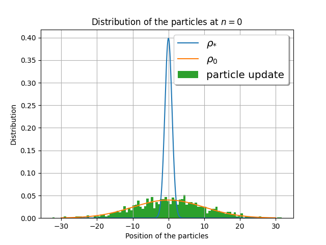
(a)

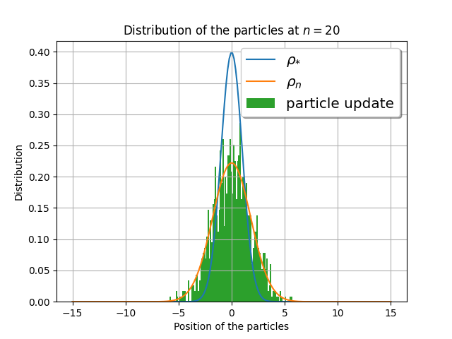
(b)

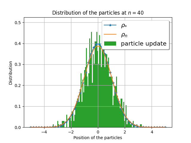
(c)

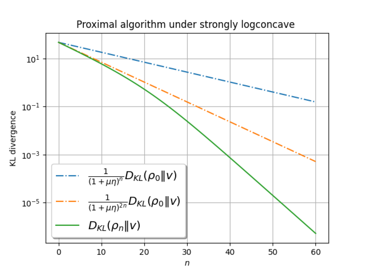
(d)

Figure 1: Wasserstein proximal algorithm on the KL divergence with $\nu=\exp(-\left\|\theta\right\|^{2}/2)$.

In Figure 1, the distribution of particles, represented by the histogram, approximates $\rho_{n}$ and converges to $\rho^{*}$ after several iterations (approximately  40 iterations in this experiment). The linear converge result of $D_{KL}(\rho_{n}\|\nu)$ in Figure 1(d) demonstrates a sharper bound holds for $\mu$-convex objective with respect to [37, 7], as Corollary 3.8 suggests.

4.2 Mean-field neural network training with entropy regularization

In practice, the optimization problem (12) typically lacks an explicit solution. Therefore, we can use particle methods to approximate the time-evolving probability distributions, and we can solve an approximate $T^{n+1}$ using functional approximation methods. When applied to our entropy-regularized total objective of mean-field neural network (9), the functional approximation method can be expressed as,

$$\begin{gathered}T^{n+1}=\arg\min_{T}\ \dfrac{1}{N}\sum_{i=1}^{N}l(\dfrac{1}{m}\sum_{j=1}^{m}\varphi(T(\theta_{j}^{n}),x_{i}),y_{i})+\dfrac{\lambda}{m}\sum_{j=1}^{m}\left\|T(\theta_{j}^{n})\right\|^{2}\\ \qquad\qquad\qquad-\dfrac{\tau}{m}\sum_{j=1}^{m}\log|\det\nabla T(\theta_{j}^{n})|+\dfrac{1}{2m\xi}\sum_{j=1}^{m}\left\|T(\theta_{j}^{n})-\theta_{j}^{n}\right\|^{2}\end{gathered}$$ (17)

where the change of variable for entropy [25] is utilized. In our work, we specifically employ a shallow neural network to learn the optimal transport map $T^{n+1}$ at each iteration, using the right-hand side of (17) as the loss function.

Experiments. In our experiments, we aim to optimize the MFLD entropy-regularized total objective (9) with $\varphi(\theta,x)=\tanh(\theta^{T}x)$ for $\theta,x\in\Theta$. The parameters are set as $d=2$,$\lambda=0.1$, $\tau=\{0.04,0.1\}$, with the number of particles $m=100$ and a discretized step size of $\xi=0.1$. We generate $N=1000$ training data samples using a teacher model $y=sin(\alpha^{T}x)$, where $x\sim\mathcal{N}(0,I)$. Our goal is to compare the proximal algorithm with the neural network-based functional approximation (17) with the noisy gradient descent algorithm (5).

We first randomly generated a dataset and then conducted 5 repeated experiments for both $\tau=0.04$ and $\tau=0.1$ on the same generated data. For each experiment, a new weight empirical distribution is generated from standard Gaussian distribution, and both algorithms will use the same weight as the initial value. For the learning of the optimal transport map, we train a one-hidden layer fully-connected neural network of the form $g(\theta)={W}_{2}\sigma(W_{1}\theta)$ for each iteration using Adam optimizer with learning rate 0.004, where $W_{1}\in\mathbb{R}^{q\times d}$, ${W}_{2}\in\mathbb{R}^{d\times q}$ where $\sigma(\cdot)=ReLU(\cdot)$ and $q=1000$.

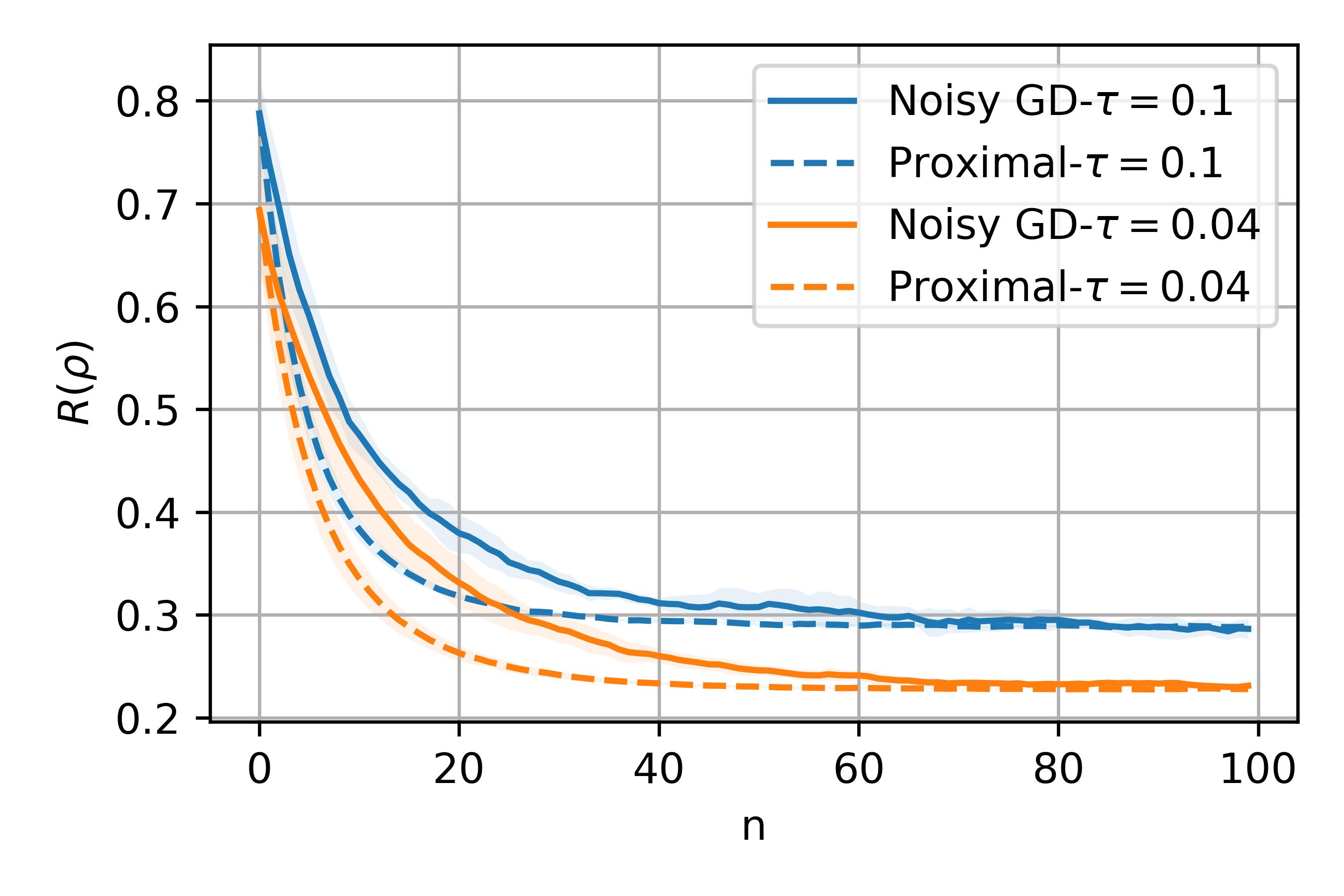
(a)

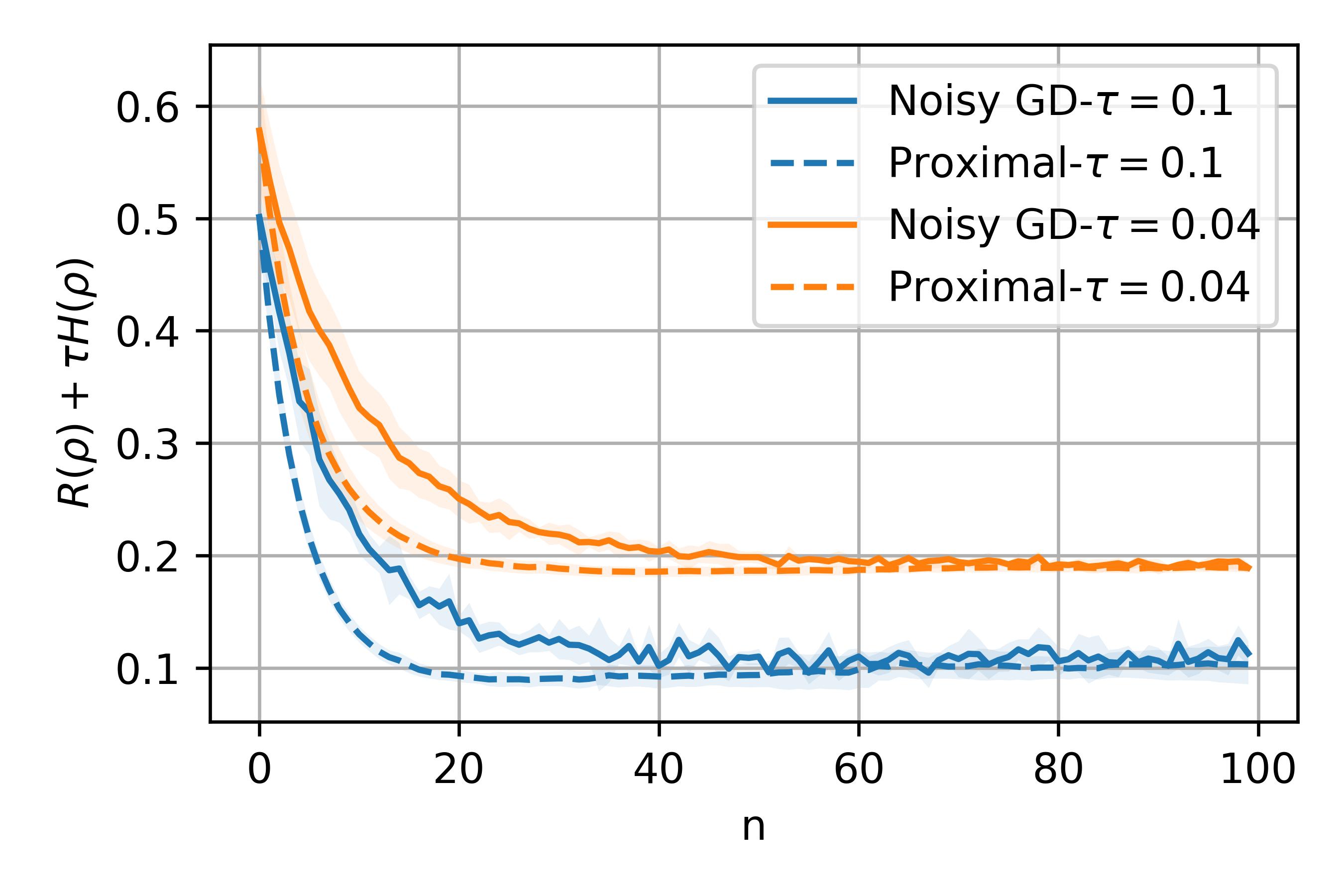
(b)

(c)

(d)

Figure 2: Wasserstein proximal algorithm on MFLD objective. Note that for Figure 2(c) and Figure 2(d), the y-axis is on log-scale.

In Figure 2(a) and Figure 2(b), we observe that both the $L^{2}$-regularized loss $R$ and the total objective $F=R+\tau\int_{\Theta}\rho log\rho$ converge under two algorithms, where the nearest neighbor estimator [17] is used to estimate $\int_{\Theta}\rho\log\rho$. To better depict the convergence rate of the Wasserstein proximal algorithm and the Langevin algorithm (forward time-discretization of MFLD), we obtain a reference $\tilde{\rho}_{\tau}^{*}$ of $\rho^{*}$, by running the noisy gradient descent algorithm with very small step size $10^{-3}$ and $m=1000$ particles. In the early training phase of both algorithms, $\mathcal{W}_{2}^{2}(\rho_{n}^{m},\tilde{\rho}_{\tau}^{*})$ is dominated by $\mathcal{W}_{2}^{2}(\rho_{n}^{m},{\rho}^{*})$ and exhibits a linear convergence above the black dash-dot line as shown in Figure 2(c) and Figure 2(d). Within this phase, the Wasserstein proximal algorithm demonstrates a faster linear rate thanks to the unbiased linear convergence nature of $\mathcal{W}_{2}^{2}(\rho_{n}^{m},\rho^{*})$ (cf. Corollary 3.5). However, both algorithm has similar bias at convergence, for which we conjecture that the particle discretization error of $\rho_{n}^{m}$ dominates $\mathcal{W}_{2}^{2}(\rho_{n}^{m},\tilde{\rho}_{\tau}^{*})$ while close to convergence. We validate our conjecture through further experiments and discussions in Appendix D.1.

5 Conclusion

In this work, we provided a convergence analysis of the Wasserstein proximal algorithm without assuming any geodesic convexity, which improves upon the existing rates when strong geodesic convexity indeed holds. We also analyzed the inexact gradient variant under an extra geodesic semiconvexity condition. Applying to the proximal training of mean-field neural networks, linear convergence of the entropy-regularized total objective is guaranteed, which is faster than the noisy gradient descent algorithm as observed in our empirical experiments. One future work would be the study of particle discretization effect of the Wasserstein proximal algorithm in the setting of MFLD [21, 12].

Appendix A Backgound on Optimal Transport and Wasserstein Space

A.1 Wasserstein distance and optimal transport

The squared 2-Wasserstein distance is defined as the solution to the Kantorovich problem

$$\mathcal{W}_{2}^{2}(\rho,\tilde{\rho}):=\min_{\pi\in\Pi(\rho,\tilde{\rho})}\int_{\Theta\times\Theta}\left\|\theta-\tilde{\theta}\right\|^{2}d\pi(\theta,\tilde{\theta}),$$

where $\Pi(\rho,\tilde{\rho})\subset\mathcal{P}_{2}(\Theta\times\Theta)$ is the set of all coupling distributions with marginals $\rho$ and $\tilde{\rho}$. The optimal solution $\pi^{*}$ is called the optimal transport plan. When $\rho\in\mathcal{P}_{2}^{a}(\Theta)$, it is known from Brenier’s theorem that the solution $T_{\rho}^{\tilde{\rho}}$ of Monge’s problem exists, and the optimal transport plan is $\pi^{*}=(\mathbf{id},T_{\rho}^{\tilde{\rho}})_{\#}\rho$.

A.2 Wasserstein subdifferential and $\mu$-convex functionals

Definition A.1 (Frechet subdifferential, [Definition 10.1.1 [1]]).

Let $F:\mathcal{P}_{2}(\Theta)\rightarrow(-\infty,+\infty]$ be proper, lower semicontinuous, and let $\rho\in D(|\partial F|)$ where $|\partial F|(\rho)$ denotes the metric slope [1]. We say that $\mathbf{v}\in L^{2}(\rho;\Theta)$ belongs to the Frechet subdifferential $\partial F(\rho)$ of $F$, written as $\mathbf{v}\in\partial F(\rho)$, if

$$F(\tilde{\rho})\geq F(\rho)+\int_{\Theta}\langle\mathbf{v}(\theta),T_{\rho}^{\tilde{\rho}}(\theta)-\theta\rangle d\rho(\theta)+o(\mathcal{W}_{2}(\rho,\tilde{\rho})).$$

And $\mathbf{v}$ is called strong subdifferential. Also, $\mathbf{v}\in\partial F(\rho)$ with minimal $\left\|\cdot\right\|_{L_{2}(\rho)}$ norm is denoted as $\partial^{\circ}F(\rho)$, and it is unique, see [Lemma 10.1.5, [1]].

Definition A.2 (First variation).

Let $F:\mathcal{P}_{2}(\Theta)\rightarrow(-\infty,+\infty]$ be proper, lower semicontinuous. Let $\rho\in\mathcal{P}_{2}(\Theta)$, the first variation $\frac{\delta F}{\delta\rho}(\rho):\Theta\rightarrow\mathbb{R}$ exists if,

$$\dfrac{d}{d\varepsilon}F(\mu+\varepsilon\chi)\Big{|}_{\varepsilon=0}=\int\dfrac{\delta F}{\delta\rho}(\rho)d\chi$$

for any perturbation $\chi=\tilde{\rho}-\rho$ with $\tilde{\rho}\in\mathcal{P}_{2}(\Theta)$.

Definition A.3 ($\mu$-convexity along geodesic, [Section 10.1.1, [1]]).

A proper, lower semicontinuous functional $F$ is said to be $\mu$-convex along geodesic ($\mu\in\mathbb{R}$) at $\rho\in\mathcal{D}(F)\cap D(|\partial F|)$, if for all $\tilde{\rho}\in\mathcal{D}(F)$,

$$F(\tilde{\rho})\geq F(\rho)+\int_{\Theta}\langle\mathbf{v}(\theta),T_{\rho}^{\tilde{\rho}}(\theta)-\theta\rangle d\rho(\theta)+\dfrac{\mu}{2}{\mathcal{W}_{2}^{2}(\rho,\tilde{\rho})},$$ (18)

where $\mathbf{v}\in\partial F(\rho)$. In particular, if $\mu\geq 0$, we call F is geodesically convex; If $\mu<0$, we call $F$ is geodesically semiconvex. We refer to [Section 9, [1]] for definitions of $\mu$-convexity (and semiconvexity) in Euclidean space, which are similar to the definition above.

Definition A.4 (Weak convergence).

Let $\mathcal{C}_{b}(\Theta)$ be the set of all continuous bounded functions on $\Theta$ and $\mathcal{M}(\Theta)$ be the set of all finite signed measures on $\Theta$. We say that $\rho_{k}\in\mathcal{M}(\Theta)$ converges to $\rho\in\mathcal{M}(\Theta)$ weakly if for every $\phi\in\mathcal{C}_{b}(\Theta)$,

$$\lim_{k\rightarrow\infty}\int_{\Theta}\phi d\rho_{k}=\int_{\Theta}\phi d\rho.$$

The weak convergence is also called narrow convergence in the literature [28].

Appendix B Technical Lemmas

Lemma B.1 (Proposition 3.1 and 3.3,  [2]).

Let $(Z,d)$ be a general metric space, $z\in Z$ such that $f(z)<+\infty$, the Hopf-Lax semigroup is defined as

$$u(z,\xi)=\inf_{z^{\prime}\in Z}f(z^{\prime})+\dfrac{1}{2\xi}d(z^{\prime},z)^{2}.$$

We define

$$D_{+}(z,\xi):=\sup\mathop{\lim\sup}_{n\rightarrow\infty}d(z,z_{n}^{\prime}),\qquad D_{-}(z,\xi):=\inf\mathop{\lim\inf}_{n\rightarrow\infty}d(z,z_{n}^{\prime}),$$

where the supremum and the infimum run among all minimizing sequences $(z_{n}^{\prime})$. For $z\in Z$ such that $f(z)<+\infty$, we define $t^{*}(z)=\sup\{t>0:u(t,\xi)>-\infty\}$. Then if $f(z)<+\infty$, we have

(a) $D_{+}(z,\xi)=D_{-}(z,\xi)$ holds for $\xi\in(0,t^{*}(z))$ except for at most countable exceptions;

(b) If and only if $D_{+}(z,\xi)=D_{-}(z,\xi)$, the map $\xi\rightarrow u(z,\xi)$ is differentiable in $(0,t^{*}(z))$ and

$$\dfrac{d}{d\xi}u(z,\xi)=-\dfrac{D_{+}(z,\xi)}{2\xi^{2}}=-\dfrac{D_{-}(z,\xi)}{2\xi^{2}}.$$

Lemma B.2 (Existence of minimizer).

If $F:\mathcal{P}_{2}(\Theta)\rightarrow(-\infty,\infty]$ is weakly lower semicontinuous, then proximal algorithm (2) admits a minimizer.

Proof.

The proof is essentially contained in [Section 10.1, [1]]. For the sake of completeness, we provide a proof here. We only need to show $\mathcal{B}_{r}(\rho)=\{\nu|\mathcal{W}_{2}^{2}(\rho,\nu)<r\}$ is weakly-precompact for any fixed $r>0$. By Prokhorov’s theorem, it suffices to prove the tightness of $\mathcal{B}_{r}(\rho)$, i.e., there is a sequence of compact sets $(K_{i})_{i\in\mathbb{N}}$ such that

$$\nu(\Theta\backslash K_{i})\leq 1/i,\forall\nu\in\mathcal{B}_{r}(\rho).$$

We prove for any $\varepsilon>0$, we can find compact set $K$ such that

$$\nu(\Theta\backslash K)\leq\varepsilon,\forall\nu\in\mathcal{B}_{r}(\rho).$$

by contradiction. Assume there exists $\varepsilon$, for any compact $K$, there exists $\nu\in\mathcal{B}_{r}(\rho)$ such that $\nu(\Theta\backslash K)>\varepsilon$. As a singleton $\{\rho\}$ constitutes a tight family, we can find a compact set $K_{\rho,\varepsilon}$ such that

$$\rho(K_{\rho,\varepsilon})<\varepsilon.$$

We define a compact set $U_{R}=\{\tilde{\theta}|argmin_{\theta\in K_{\rho,\varepsilon}}\left\|\theta-\tilde{\theta}\right\|^{2}\leq R,\}$. Then there exists $\nu$ such that $\nu(\Theta\backslash U_{3r/\varepsilon})>\varepsilon$. However, $\mathcal{W}_{2}^{2}(\rho,\nu)\geq 3r$, contradiction. Furthermore, note that since $\Theta$ is not compact, $\mathcal{B}_{r}(\rho)$ under the Wasserstein metric is not compact. ∎

Lemma B.3 (Conditions on weakly lower semicontinuity).

If $F:\mathcal{P}_{2}(\Theta):\rightarrow(-\infty,+\infty]$ is proper, lower semicontinuous (with respect to $\mathcal{W}_{2}$ topology), and $\mu$-convex ($\mu\in\mathbb{R}$) along generalized geodesics , then $F$ is weakly lower semicontinuous.

Proof of Lemma B.3.

See Section 10.3 in [1]. ∎

Remark B.4.

We give several examples that the functional $F$ satisfies weakly lower continuity.

• If $f:\Theta\rightarrow(-\infty,+\infty]$ is lower semicontinuous, and $\mu$-convex ($\mu\in\mathbb{R}$) in Euclidean sense, then Lemma B.3 implies that $F=\int_{\Theta}fd\rho$ is weakly lower semicontinuous.

• If $f:\Theta\rightarrow(-\infty,+\infty]$ is lower semicontinuous and bounded from below, then $F=\int_{\Theta}fd\rho$ is weakly lower semicontinuous, [Example 9.3.1, [1]].

• For conditions that ensure the weakly lower semicontinuity of internal energy, we refer to [Section 9.3, [1]] for details. Specifically, $\int_{\Theta}\rho log\rho$ is weakly lower semicontinuous.

Lemma B.5 (Satisfication of Assumption 2 on $\mathcal{P}_{2}(\Theta)$ with compact set $\Theta$).

Under Assumption 1, if $\Theta$ is compact, then Assumption 2 holds.

Proof.

By [Proposition 7.17, [28]], when $\Theta$ is compact, for fixed $\rho\in\mathcal{P}_{2}(\Theta)$, the first variation of $\mathcal{W}_{2}(\cdot,\rho)$ is well-defined for all $\tilde{\rho}\in\mathcal{P}_{2}^{a}(\Theta)$. Similar to [Proposition 8.7, [28]], by standard calculus of variation followed by gradient operation, we have

$$\nabla\dfrac{\delta F}{\delta\rho}(\rho_{\xi})=\dfrac{T_{\rho_{\xi}}^{\rho}-\mathbf{id}}{\xi}.$$

See [Lemma B.1, [36]] for similar arguments. Therefore, Assumption 2 holds. If $\Theta$ is not compact, the first variation of $\mathcal{W}_{2}$ distance is not well defined. ∎

Lemma B.6.

Assume $u:[0,\xi]\rightarrow(0,+\infty)$ is a decreasing function, $\partial_{t}u(t)\leq-C(t)u(t)$ almost everywhere for $t\in[0,\xi]$, $C(t)>0$ for every $t\in[0,\xi]$, then

$$u(\xi)\leq u(0)\exp\left(\int_{0}^{\xi}-C(t)dt\right).$$

Remark B.7.

Lemma B.6 extends the classical Gronwall lemma, which requires everywhere differentiability, to the case with almost everywhere differentiability and monotonicity.

Proof.

By the monotonicity of $u(t)$ we construct a function $g(t)=\ln(u(t))$. It is a decreasing function and $\dfrac{dg(t)}{dt}=\dfrac{\partial_{t}u(t)}{u(t)}\leq-C(t)$ almost everywhere on $[0,\xi]$. By properties of Lebesgue integral, we have

$$\int_{0}^{\xi}\dfrac{dg(t)}{dt}dt\leq\int_{0}^{\xi}-C(t)dt.$$

Since $g$ is decreasing, by [Proposition 6.6, [20]],

$$g(\xi)-g(0)\leq\int_{0}^{\xi}\dfrac{dg(t)}{dt}dt.$$

Thus,

$$u(\xi)\leq u(0)\exp\left(\int_{0}^{\xi}-C(t)dt\right).$$

∎

Lemma B.8.

Assume $T_{\overline{\rho}_{n}}^{\overline{\rho}_{n+1}}$ is $C^{2}$ diffeomorphism. If $\overline{\rho}_{n}\in\mathcal{C}^{1}(\Theta)$, then $\overline{\rho}_{n+1}\in\mathcal{C}^{1}(\Theta)$.

Proof.

The change variable formula of probability density is,

$$T_{\#}{\rho}(\theta)=\rho(T^{-1}(\theta))\cdot|detD(T^{-1})(\theta)|$$

where $D(T^{-1})$ is the Jacobian matrix of $T^{-1}$. Since $T$ is a $\mathcal{C}^{2}$ diffeomorphism, then $T^{-1}$ is $\mathcal{C}^{2}$ mapping. Thus, $\rho\circ(T^{-1})$ is $\mathcal{C}^{1}(\Theta)$. Since $T^{-1}$ is diffeomorphism, then $D(T^{-1})$ is not singular and $|detD(T^{-1})|$ is $C^{1}(\Theta)$. And thus $T_{\#}\rho$ is $\mathcal{C}^{1}(\Theta)$. ∎

Remark B.9.

We have an example from normalizing flow that can be $\mathcal{C}^{2}$ diffeomorphism. Real NVP [11] has the following structure,

$$T(\theta_{1:\tilde{d}}) =\theta_{1:\tilde{d}}$$

$$T(\theta_{\tilde{d}+1:d}) =\theta_{\tilde{d}+1:d}*exp(s(\theta_{1:\tilde{d}})+t(\theta_{1:\tilde{d}}))$$

where $*$ refers to the pointwise product. $T$ is naturally reversible (The Jacobian matrix is always non-singular) and the reverse is,

$$T^{-1}(\theta_{1:\tilde{d}}) =\theta_{1:\tilde{d}}$$

$$T^{-1}(\theta_{\tilde{d}+1:d}) =(\theta_{\tilde{d}+1:d}-t(\theta_{1:\tilde{d}}))*exp(-s(\theta_{1:\tilde{d}}))$$

It is not hard to see that if $s(\cdot):\mathbb{R}^{\tilde{d}}\rightarrow\mathbb{R}^{d-\tilde{d}}$ and $t(\cdot):\mathbb{R}^{\tilde{d}}\rightarrow\mathbb{R}^{d-\tilde{d}}$ are $\mathcal{C}^{2}$ maps (i.g. represented by fully neural network with smooth activation function), then $T$ is restricted to be $\mathcal{C}^{2}$ diffeomorphism.

Lemma B.10.

Under Assumption 3, if $\overline{\rho}_{n}\in\mathcal{C}^{1}(\Theta)$ and $\overline{\rho}_{n+1}$ is the exact solution of the Wasserstein proximal algorithm (2), then $\beta_{n+1}=0$.

Proof.

Since $\overline{\rho}_{n+1}$ is the exact solution of (2), then $\overline{\rho}_{n+1}\in D(|\partial F|)$ and $\frac{T_{\overline{\rho}_{n+1}}^{\overline{\rho}_{n}}-\mathbf{id}}{\xi}\in\partial F(\overline{\rho}_{n+1})$ by [Lemma 10.1.2, [1]]. As $\overline{\rho}_{n+1}\in\mathcal{C}^{1}(\Theta)$, then $\nabla\dfrac{\delta F}{\delta\rho}(\overline{\rho}_{n+1})$ is the unique strong subdifferential by [Lemma 10.4.1, [1]]. Therefore,

$${T_{\overline{\rho}_{n+1}}^{\overline{\rho}_{n}}-\mathbf{id}}-\xi\nabla\frac{\delta F}{\delta\rho}(\overline{\rho}_{n+1})=0$$

∎

Appendix C Proofs

Proof of Lemma 3.1.

Lemma B.2 guarantees the existence of a minimizer of the JKO scheme or proximal algorithm. Thus we can define

$$z_{\xi}=\arg\min_{z\in\mathcal{P}_{2}(\mathbb{R}^{d})}u(z,\xi).$$

Then Lemma B.1 implies that $D_{+}(z,\xi)=D_{-}(z,\xi)=d(z,z_{\xi})$ in $(0,t^{*}(z))$ except for at most countable exceptions, from which we can conclude the desired Lemma 3.1. ∎

Definition C.1 (Uniform log-Sobolev inequality).

There is a constant $\mu>0$ such that for any $\rho\in\mathcal{P}_{2}(\Theta)$, its Gibbs proximal distribution $q_{\rho}$ defined as,

$$q_{\rho}(\theta)\propto\exp\left(-{1\over\tau}{\delta R\over\delta\rho}(\rho)(\theta)\right)$$

satisfies the log-Sobolev inequality (7) with the constant $\mu$.

Proof of Corollary 3.5.

We divide our proof into four parts,
(1) Firstly, we prove the satisfaction of Assumption 1 and the geodesic semiconvexity of $F_{\tau}$;
(2) Secondly, we prove the PL inequality;
(3) Thirdly, we prove the satisfaction of Assumption 2 by showing that $\nabla\frac{\delta F_{\tau}}{\delta\rho}(\rho_{\xi})=\partial^{\circ}F_{\tau}(\rho_{\xi})$;
(4) With the previous three parts, we can get the linear convergence of function value. The last part is devoted to obtain a convergence rate of $\mathcal{W}_{2}$ distance using some structure of MFLD.

Our proof is as follows,
(1) The weakly lower semicontinuity of $F_{\tau}$ is verified in [Section 5.1, [6]]. The geodesic semiconvexity follows from [Lemma A.2, [6]] and the proof relies on (19) below.

(2) Now we prove PL inequality. The training risk $R:\mathcal{P}_{2}(\Theta)\rightarrow(-\infty,+\infty]$ has linear convexity if the loss function $l$ is convex (in the Euclidean sense). By [Proposition 5.1,  [6]], the $L^{2}$-regularized training risk $R$ in (4) satisfies the uniform LSI assumption [Assumption 3, [6]]. Next, we shall show that these assumptions imply the relaxed PL-inequality defined in (13). By the entropy sandwich bound [Lemma 3.4,  [6]] (which relies on linear convexity of $F_{\tau}$),

$$\tau D_{\mathrm{KL}}(\rho\|q_{\rho})\geq F_{\tau}(\rho)-F_{\tau}(\rho^{*}).$$

Therefore,

$$\int_{\Theta}\left\|\nabla\frac{\delta F_{\tau}}{\delta\rho}(\rho)\right\|^{2}d\rho =\int_{\Theta}\left\|\nabla\frac{\delta{R}}{\delta\rho}(\rho)+\tau\nabla\log(\rho)\right\|^{2}d\rho$$

$$=\tau^{2}J_{q_{\rho}}(\rho)\geq 2\mu_{\tau}\tau^{2}D_{\mathrm{KL}}(\rho\|q_{\rho})\geq 2\mu_{\tau}\tau(F_{\tau}(\rho)-F_{\tau}(\rho^{*})),$$

Thus, the functional $F_{\tau}$ satisfies the Wasserstein PL-inequality with parameter $\tau\mu_{\tau}$.

(3) Under Assumption 1, $(T_{\rho_{\xi}}^{\rho}-\mathbf{id})/\xi$ is a strong subdifferential at $\rho_{\xi}\in\mathcal{P}_{2}^{a}(\Theta)$, and $\rho_{\xi}\in D(|\partial F_{\tau}|)$ by [Lemma 10.1.2, [1]]. To prove that Assumption 2 holds, we only need to prove that,

If $\rho\in D(|\partial F_{\tau}|)\cap\mathcal{P}_{2}^{a}(\Theta)$, then $\nabla\frac{\delta F_{\tau}}{\delta\rho}(\rho)=\partial^{\circ}F_{\tau}(\rho)$.

Our proof for (3) below highly relies on the proof of [Theorem 10.4.13, [1]].
Step 1. We first need to derive some conditions similar to [(10.4.58), (10.4.59), [1]]. Under the assumptions of Corollary 3.5, $R$ satisfies the following smoothness condition with $\tilde{L}>0$ by [Proposition 5.1, [6]].

$$\forall\theta,\tilde{\theta}\in\Theta,\forall\rho,\tilde{\rho}\in\mathcal{P}_{2}(\Theta),\quad\left\|\nabla\dfrac{\delta{R}}{\delta\rho}(\rho)(\theta)-\nabla\dfrac{\delta{R}}{\delta\rho}(\tilde{\rho})(\tilde{\theta})\right\|\leq\tilde{L}(\|\theta-\tilde{\theta}\|_{2}+\mathcal{W}_{2}(\rho,\tilde{\rho})).$$ (19)

By [Lemma A.2, [6]], relying on (19), choosing $\mathbf{r}=\mathbf{id}+\mathbf{t}$ with $\mathbf{t}\in C_{c}^{\infty}(\Theta)$,

$$\lim_{t\rightarrow 0}\dfrac{R((\mathbf{id}+t\mathbf{t})_{\#}\rho)-R(\rho)}{t}=\int_{\Theta}\langle\nabla\dfrac{\delta R}{\delta\rho}(\rho),\mathbf{r}-\mathbf{id}\rangle d\rho.$$ (20)

(20) is the key condition similar to [(10.4.58), (10.4.59), [1]] that we want to obtain. Furthermore, a by-product is that (20) suggests that $\nabla\frac{\delta R}{\delta\rho}(\rho)$ is a (unique) strong subdifferential and $\left\|\nabla\frac{\delta R}{\delta\rho}(\rho)\right\|_{L_{2}(\rho)}=\left|\partial R\right|(\rho)$ for all $\rho\in\mathcal{P}_{2}^{a}(\Theta)$, see [Lemma A.2, [6]]. It is not hard to verify that $\left\|\nabla\frac{\delta R}{\delta\rho}(\rho)\right\|_{L_{2}(\rho)}$ is finite at any $\rho\in\mathcal{P}_{2}(\Theta)$ because (19) ensures 2-growth of $\left\|\nabla\frac{\delta R}{\delta\rho}(\rho)(\cdot)\right\|^{2}$.

In Step 2, we conduct a proof similar to [Theorem 10.4.13, [1]].

Step 2. By [Lemma 10.4.4, [1]], (20), and the fact that $\rho\in\mathcal{P}_{2}^{a}(\Theta)\cap D(|\partial F|)$, for $\mathbf{t}\in C_{c}^{\infty}(\Theta)$

$$-\int_{\Theta}\tau\rho\nabla\cdot\mathbf{t}d\theta+\int_{\Theta}\langle\nabla\dfrac{\delta R}{\delta\rho}(\rho),\mathbf{t}\rangle d\rho\geq-|\partial F_{\tau}(\rho)|\left\|\mathbf{t}\right\|_{L_{2}(\rho)}.$$

By (19), $\forall\theta,\tilde{\theta}\in\Theta,\forall{\rho}\in\mathcal{P}_{2}(\Theta)$,

$$\quad\left\|\nabla\dfrac{\delta{R}}{\delta\rho}(\rho)(\theta)-\nabla\dfrac{\delta{R}}{\delta\rho}(\rho)(\tilde{\theta})\right\|\leq\tilde{L}(\|\theta-\tilde{\theta}\|_{2}).$$

Therefore, $\nabla\dfrac{\delta{R}}{\delta\rho}(\rho)(\cdot)$ is Lipschitz and locally bounded. Therefore, following the same argument of [Theorem 10.4.13, [1]], we obtain that

$$\nabla\dfrac{\delta F_{\tau}}{\delta\rho}(\rho)=\tau\dfrac{\nabla\rho}{\rho}+\nabla\dfrac{\delta R}{\delta\rho}(\rho)\in L_{2}(\rho)\text{ and }{\left\|\nabla\dfrac{\delta F_{\tau}}{\delta\rho}(\rho)\right\|_{L_{2}(\rho)}\leq|\partial F_{\tau}(\rho)|}.$$

where we define $\frac{\nabla\rho}{\rho}=0$ if $\rho(\theta)=0$. Furthermore, it is straightforward to prove $\nabla\dfrac{\delta F_{\tau}}{\delta\rho}(\rho)\in\partial F_{\tau}(\rho)$. Since $\rho\in D(|\partial F_{\tau}|)$ and $\rho\in D(|\partial R|)$, we have $\rho\in D(|\partial H_{\tau}|)$ where $H_{\tau}(\rho)=\int_{\Theta}\tau\rho log\rho$. Therefore, $\tau\frac{\nabla{\rho}}{\rho}\in\partial H_{\tau}(\rho)$ [Theorem 10.4.6, [1]]. With $\nabla\dfrac{\delta R}{\delta\rho}(\rho)\in\partial R(\rho)$, we have proved that $\nabla\dfrac{\delta F_{\tau}}{\delta\rho}(\rho)\in\partial F_{\tau}(\rho)$. Thus, $\nabla\dfrac{\delta F_{\tau}}{\delta\rho}(\rho)=\partial^{\circ}F_{\tau}(\rho)$.

(4) With the previous three parts, we can get (14) with Theorem 3.4. Next, we prove (15). Using [Lemma 3.4, [6]] once again, we get

$$\tau D_{\mathrm{KL}}(\rho\|\rho^{*})\leq F_{\tau}(\rho)-F_{\tau}(\rho^{*})\leq\tau D_{\mathrm{KL}}(\rho\|q_{\rho}).$$

Since $\rho^{*}$ also satisfies $\mu_{\tau}$-LSI, by Talagrand’s inequality, we have

$$\mathcal{W}_{2}^{2}(\rho^{*},\rho_{n})\leq\dfrac{2}{\mu_{\tau}}D_{\mathrm{KL}}(\rho_{n}\|\rho^{*})\leq\dfrac{2}{\mu_{\tau}\tau}(F_{\tau}(\rho_{n})-F_{\tau}(\rho^{*}))\leq\dfrac{2}{\mu_{\tau}\tau}(F_{\tau}(\rho_{0})-F_{\tau}(\rho^{*}))(\dfrac{1}{1+\mu_{\tau}\tau\xi})^{2n}.$$

∎

Proof of Corollary 3.6.

Similar to proof of Corollary 3.5, we divide the proof into four parts.

(1) If $f$ is semiconvex and lower-semicontinuous, then $\int_{\Theta}fd\rho$ is weakly lower semicontinuous by Remark B.4. In addition, $\int_{\Theta}\log\rho d\rho$ is also weakly lower semicontinuous by Remark B.4. Thus, $F$ is weakly lower continuous, and Assumption 1 satisfies.

Furthermore, $\int_{\Theta}fd\rho$ is semiconvex along geodesics and $\int_{\Theta}\log\rho d\rho$ is convex along geodesics, see [Section 9.3, [1]]. Thus, $F$ is semiconvex along geodesics.

(2) The PL inequality directly follows from LSI condition.

(3) We prove that Assumption 2 is satisfied by showing $\nabla\frac{\delta F}{\delta\rho}(\rho_{\xi})=\partial^{\circ}F(\rho_{\xi})$. [Theorem 10.4.13, [1]] already incorporates KL divergence as a special case: Assume $f$ is semiconvex and lower semicontinuous, and $\{\theta|V(\theta)<\infty\}$ is not empty. Then for $F(\rho)=\int_{\Theta}fd\rho+\int_{\Theta}\rho log\rho$ (here we assume the interaction energy to be 0), if $\rho\in D(|\partial F|)\cap\mathcal{P}_{2}^{a}(\Theta)$, then $\nabla\frac{\delta F}{\delta\rho}(\rho)=\nabla V+\nabla\log(\rho)=\partial^{\circ}F(\rho)$, where we assume $\nabla log(\rho)(\theta)=0$ if $\rho(\theta)=0$. With Assumption 1 to guarantee $\rho_{\xi}\in\mathcal{P}_{2}^{a}(\Theta)$ and [Lemma 10.1.2, [1]] to guarantee that $\rho_{\xi}\in D(|\partial F|)$, Assumption 2 holds.

(4) The convergence rate on $\mathcal{W}_{2}$ distance follows Talagrand inequality. ∎

Proof of Theorem 3.8.

In this proof, we will not invoke Assumption 2.
Step 1. We want to prove that $\mu$-geodesic convex implies, for any fixed $\rho$ and for any $\xi$,

$$F(\rho^{*})\geq F(\rho_{\xi})-\dfrac{1}{2\mu\xi^{2}}\mathcal{W}_{2}^{2}(\rho_{\xi},\rho).$$ (21)

Note $\dfrac{T_{\rho_{\xi}}^{\rho}-I}{\xi}$ is a strong subdifferential at $\rho_{\xi}$,

$$F(\tilde{\rho}) \geq F(\rho_{\xi})+\int_{\Theta}\langle\dfrac{T_{\rho_{\xi}}^{\rho}(\theta)-\theta}{\xi},T_{\rho\xi}^{\tilde{\rho}}(\theta)-\theta\rangle d\rho_{\xi}(\theta)+\dfrac{\mu}{2}{\mathcal{W}_{2}^{2}(\rho_{\xi},\tilde{\rho})}$$

$$=F(\rho_{\xi})+\int_{\Theta}\left(\langle\dfrac{T_{\rho_{\xi}}^{\rho}(\theta)-(\theta)}{\xi},T_{\rho_{\xi}}^{\tilde{\rho}}(\theta)-\theta\rangle+\dfrac{\mu}{2}\left\|T_{\rho_{\xi}}^{\tilde{\rho}}(\theta)-\theta\right\|^{2}\right)d\rho_{\xi}(\theta).$$

Then, we minimize both sides of Eqn (18) with respect to $\tilde{\rho}\in\mathcal{P}_{2}^{a}(\Theta)$. Clearly, $\rho^{*}$ minimizes the left side. For the integral term on the right-hand side, we define $T_{\rho_{\xi}}^{\tilde{\rho}}$ in the following,

$$T_{\rho_{\xi}}^{\tilde{\rho}}(\theta)-\theta=-\dfrac{1}{\mu\xi}\left(T_{\rho_{\xi}}^{\rho}(\theta)-\theta\right),\quad\rho_{\xi}\text{-}a.e.$$

then it minimizes the integral as it minimizes the term inside the integral almost everywhere. Therefore,

$$F(\rho^{*})\geq F(\rho_{\xi})-\dfrac{1}{2\mu\xi^{2}}\int_{\Theta}\left\|T_{\rho_{\xi}}^{\rho}(\theta)-\theta\right\|^{2}d\rho_{\xi}(\theta)=F(\rho_{\xi})-\dfrac{1}{2\mu\xi^{2}}W_{2}^{2}(\rho_{\xi},\rho).$$

Step 2.

$$\partial_{\xi}(u(\rho,\xi)-F^{*}) =-\dfrac{\mu}{2\xi(1+\mu\xi)}\mathcal{W}_{2}^{2}(\rho_{\xi},\rho)-\dfrac{1}{2(1+\mu\xi)\xi^{2}}\mathcal{W}_{2}^{2}(\rho_{\xi},\rho)$$ (by (11))

$$\leq-\dfrac{\mu}{2\xi(1+\mu\xi)}\mathcal{W}_{2}^{2}(\rho_{\xi},\rho)-\dfrac{\mu}{(1+\mu\xi)}(F(\rho_{\xi})-F^{*})$$ (by (21) in Step 1)

$$=-\dfrac{\mu}{1+\mu\xi}(u(\rho,\xi)-F^{*}).$$ (by Def 3.1)

Using Lemma B.6 to deal with the technique issue of almost everywhere differentiability, we have

$$u(\rho,\xi)-F^{*} \leq(u(\rho,0)-F^{*})\exp\left(\int_{0}^{\xi}-\frac{\mu}{1+\mu t}dt\right)=(F(\rho)-F^{*})\dfrac{1}{1+\mu\xi}.$$

Invoking (21) once again, we obtain that

$$(F(\rho)-F^{*})\dfrac{1}{1+\mu\xi}\geq u(\rho,\xi)-F^{*}=F(\rho_{\xi})-F^{*}+\dfrac{1}{2\xi}\mathcal{W}_{2}^{2}(\rho_{\xi},\rho)\geq(1+\mu\xi)(F(\rho_{\xi})-F^{*}).$$

Step 3. We derive a bound for $\mathcal{W}_{2}(\rho^{*},\rho_{n})$ here. Since for any $\rho\in\mathcal{D}(F)$,

$$F(\rho)-F(\rho^{*})\geq\int_{\Theta}\langle{\bf{0}},T_{\rho^{*}}^{\rho}\rangle d\rho^{*}(\theta).$$

Therefore, ${\bf{0}}$ is a strong subdifferential by definition of geodesic convexity. Thus, we have

$$F(\rho)-F(\rho^{*})\geq\int_{\Theta}\langle{\bf{0}},T_{\rho^{*}}^{\rho}\rangle d\rho^{*}(\theta)+\dfrac{\mu}{2}\mathcal{W}_{2}^{2}(\rho^{*},\rho)=\dfrac{\mu}{2}\mathcal{W}_{2}^{2}(\rho^{*},\rho).$$

by definition of $\mu$-convexity along geodesics. Therefore,

$$\mathcal{W}_{2}(\rho^{*},\rho_{n})\leq\sqrt{\dfrac{2}{\mu}F(\rho_{0})-F(\rho^{*})}\dfrac{1}{(1+\mu\xi)^{n}}.$$

∎

Proof of Theorem 3.10.

It suffices to prove the case $\xi=1/L$ because for $\xi<1/L$, a functional that is $(-L)$ geodesically convex is also $-(1/\xi)$ geodesically convex. Under Assumption 3, since we assume $\overline{\rho}_{n+1}\in D(\partial F)$, then $\nabla\frac{\delta F}{\delta\rho}(\overline{\rho}_{n+1})$ is the unique strong subdifferential. Thus,

$$F(\overline{\rho}_{n+1})-F(\overline{\rho}_{n}) \leq-\xi\int_{\Theta}\langle\nabla\dfrac{\delta F}{\delta\rho}(\overline{\rho}_{n+1}),\dfrac{T_{\overline{\rho}_{n+1}}^{\overline{\rho}_{n}}-\mathbf{id}}{\xi}\rangle d\overline{\rho}_{n+1}+\dfrac{L}{2}\mathcal{W}_{2}^{2}(\overline{\rho}_{n+1},\overline{\rho}_{n})$$

$$=-\xi\int_{\Theta}\langle\nabla\dfrac{\delta F}{\delta\rho}(\overline{\rho}_{n+1}),\nabla\dfrac{\delta F}{\delta\rho}(\overline{\rho}_{n+1})+\dfrac{1}{\xi}\beta_{n+1}\rangle d\overline{\rho}_{n+1}$$

$$\qquad\qquad+\dfrac{L}{2}\int_{\Theta}\left\|\xi\nabla\dfrac{\delta F}{\delta\rho}(\overline{\rho}_{n+1})+\beta_{n+1}\right\|^{2}d\overline{\rho}_{n+1}$$ (by Eqn 16)

$$=(-\dfrac{1}{2L}){\int_{\Theta}\left\|\nabla\dfrac{\delta F}{\delta\rho}(\overline{\rho}_{n+1})\right\|^{2}d\overline{\rho}_{n+1}}+\dfrac{L}{2}\int_{\Theta}\left\|\beta_{n+1}\right\|^{2}d\overline{\rho}_{n+1} \xi=\frac{1}{L}$$ (let )

$$\leq-\dfrac{\mu}{L}(F(\overline{\rho}_{n+1})-F(\rho^{*}))+\dfrac{L}{2}(\epsilon_{n+1}).$$ (by PL (13))

Thus,

$$(1+\dfrac{\mu}{L})(F(\overline{\rho}_{n+1})-F^{*})\leq(F(\overline{\rho}_{n})-F^{*})+\dfrac{L}{2}\epsilon_{n+1}.$$ (22)

By [Lemma 14, [36]], we set $A=\frac{1}{1+\mu/L}$, $B=\frac{L/2}{1+\mu/(L)}$.

(a) If $\epsilon_{n}\leq C_{exp}\gamma^{n}$ with $\gamma\in(0,1)$,

$$F(\overline{\rho}_{n})-F(\rho^{*})\leq A^{n}(F(\rho_{0})-F(\rho^{*}))+\dfrac{BC_{exp}}{|A-\gamma|}max\{A,\gamma\}^{n+1}.$$

(b) If $\epsilon_{n}\leq C_{poly}n^{-\zeta}$ with $\zeta>0$, there is a constant $C(\zeta,A)$,

$$F(\overline{\rho}_{n})-F(\rho^{*})\leq A^{n}(F(\rho_{0})-F(\rho^{*}))+\dfrac{BC(\zeta,A)\zeta}{n^{\zeta}}.$$

∎

Appendix D Further Numerical Experiments and Discussions

D.1 Further discussions on MFLD Experiments

As shown in Figure 3, while $m$ increases, $\mathcal{W}_{2}(\rho_{n}^{m},\tilde{\rho}_{\tau}^{*})$ at convergence decreases for both algorithms. This experiment supports our conjecture that partial discretization error dominates the bias, if we assume $\tilde{\rho}_{\tau}^{*}$ is a good approximate of $\rho^{*}$.

The particle discretization error is well studied for noisy gradient descent and a quantitative uniform-in-time propagation of chaos result for the MFLD has been established in [9]. Specifically, the ”distance” between the finite particle dynamics and the mean-field dynamics converges at rate $O(1/m)$ for all $t>0$ under the uniform LSI condition. Note that even though the “distance” in theoretical analysis of uniform propagation chaos is not simply defined to be the $\mathcal{W}_{2}$ distance between the empirical measure of finite particle dynamics and absolutely continuous measure of mean-field dynamics, it is empirically observed that the $\mathcal{W}_{2}$ distance also demonstrates similar propagation-of-chaos property in Figure 3(b). One future work would be the study of particle discretization effect of the Wasserstein proximal algorithm in the setting of MFLD [21, 12].

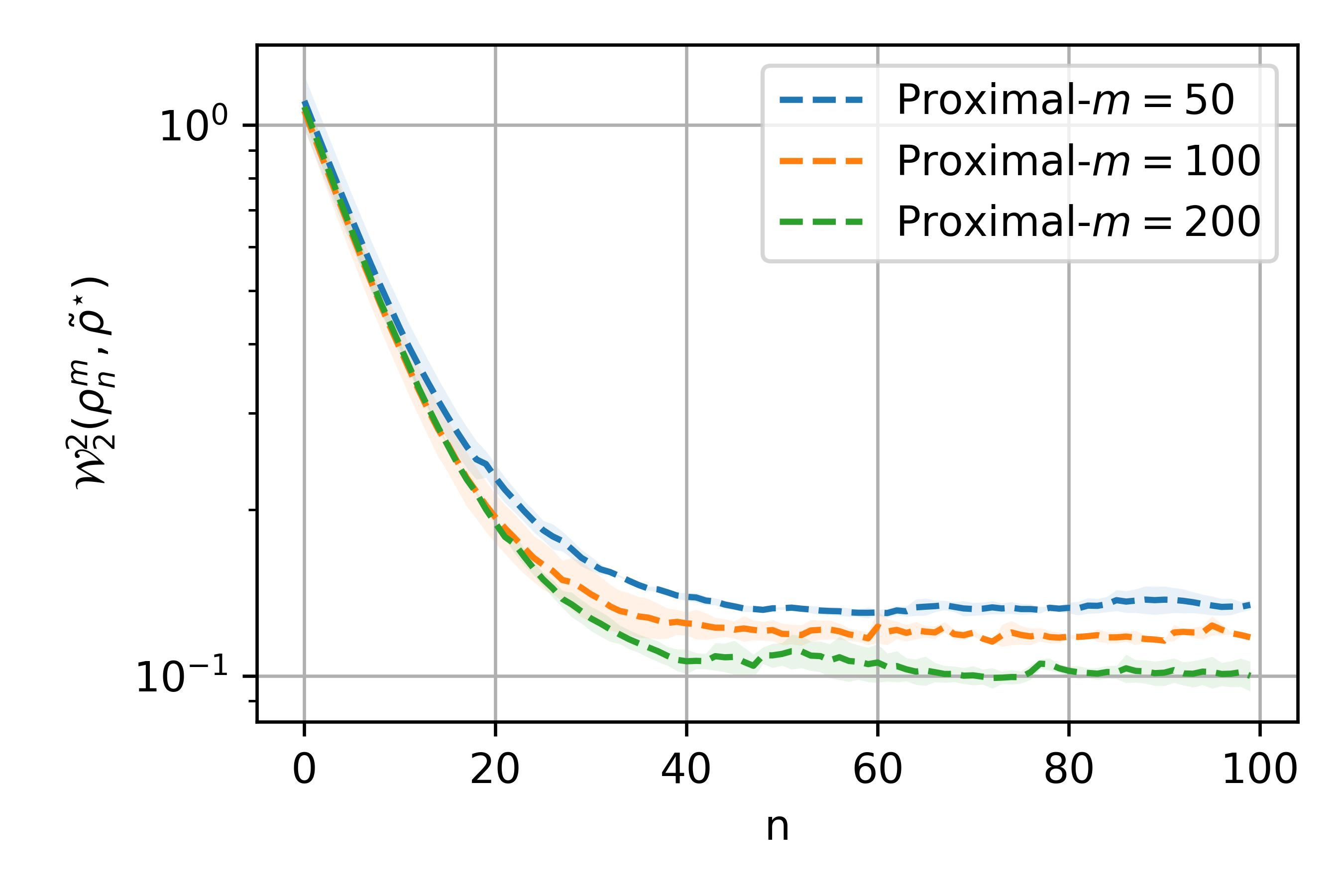
(a)

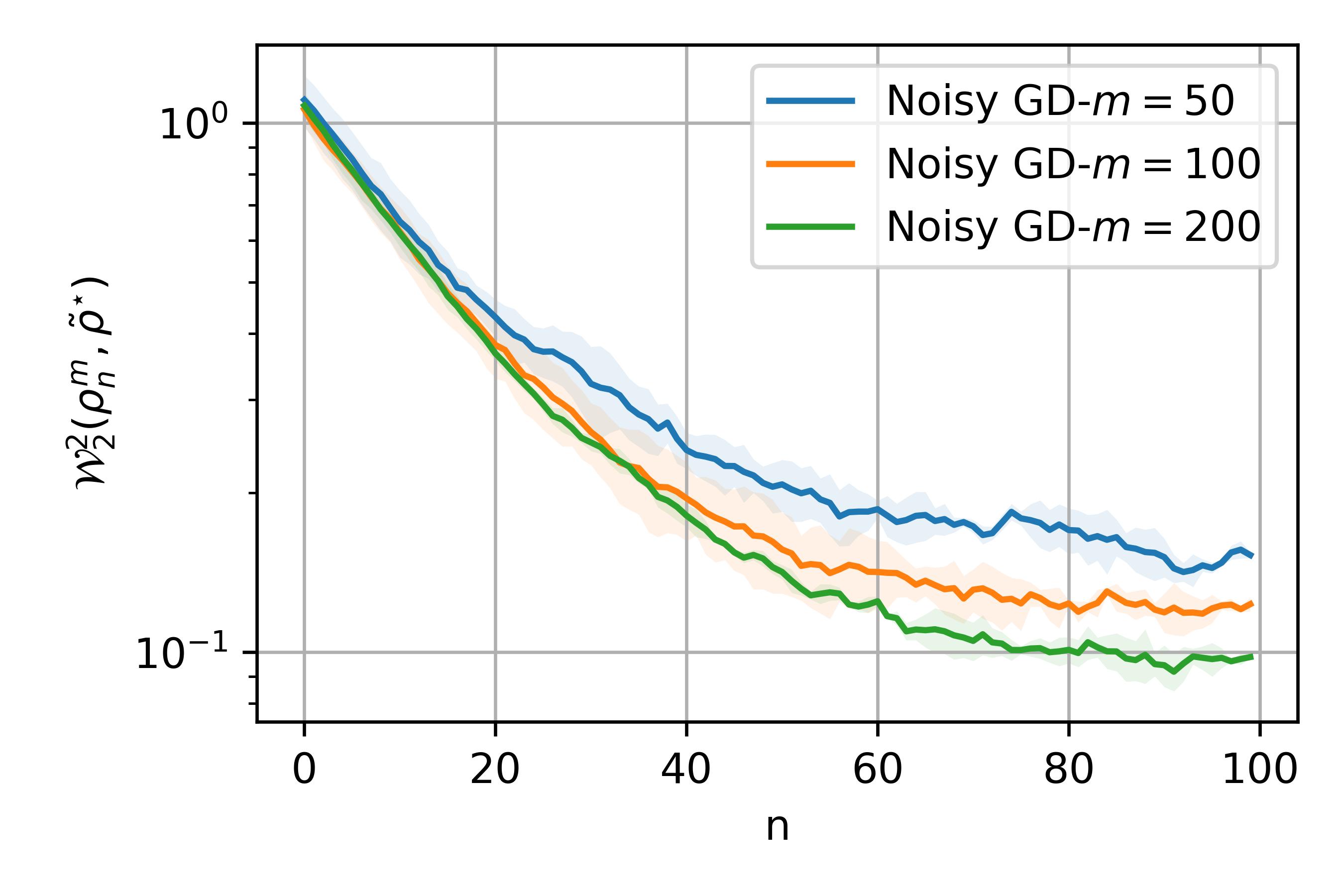
(b)

Figure 3: Particle discretization error with different number of particles. We follow all the experiment settings in Section 4.2.

References

- AGS [08] Luigi Ambrosio, Nicola Gigli, and Giuseppe Savaré. Gradient Flows: in Metric Spaces and in the Space of Probability Measures. Springer Science & Business Media, 2008.
- AGS [14] Luigi Ambrosio, Nicola Gigli, and Giuseppe Savaré. Calculus and heat flow in metric measure spaces and applications to spaces with ricci bounds from below. Inventiones mathematicae, 195(2):289–391, 2014.
- BV [23] Siwan Boufadène and François-Xavier Vialard. On the global convergence of Wasserstein gradient flow of the Coulomb discrepancy. arXiv preprint arXiv:2312.00800, 2023.
- CCSW [22] Yongxin Chen, Sinho Chewi, Adil Salim, and Andre Wibisono. Improved analysis for a proximal algorithm for sampling. In Conference on Learning Theory, pages 2984–3014. PMLR, 2022.
- CEL+ [24] Sinho Chewi, Murat A Erdogdu, Mufan Li, Ruoqi Shen, and Matthew S Zhang. Analysis of Langevin Monte Carlo from Poincaré to log-Sobolev. Foundations of Computational Mathematics, pages 1–51, 2024.
- Chi [22] Lénaïc Chizat. Mean-field Langevin dynamics : Exponential convergence and annealing. Transactions on Machine Learning Research, 2022.
- CLTX [24] Xiuyuan Cheng, Jianfeng Lu, Yixin Tan, and Yao Xie. Convergence of flow-based generative models via proximal gradient descent in Wasserstein space. IEEE Transactions on Information Theory, pages 1–1, 2024.
- CMRS [20] Sinho Chewi, Tyler Maunu, Philippe Rigollet, and Austin J Stromme. Gradient descent algorithms for Bures-Wasserstein barycenters. In Conference on Learning Theory, pages 1276–1304. PMLR, 2020.
- CRW [22] Fan Chen, Zhenjie Ren, and Songbo Wang. Uniform-in-time propagation of chaos for mean field Langevin dynamics. arXiv preprint arXiv:2212.03050, 2022.
- DMM [19] Alain Durmus, Szymon Majewski, and Błażej Miasojedow. Analysis of Langevin Monte Carlo via convex optimization. Journal of Machine Learning Research, 20(73):1–46, 2019.
- DSDB [16] Laurent Dinh, Jascha Sohl-Dickstein, and Samy Bengio. Density estimation using real NVP. arXiv preprint arXiv:1605.08803, 2016.
- FW [24] Qiang Fu and Ashia Camage Wilson. Mean-field underdamped Langevin dynamics and its spacetime discretization. In International Conference on Machine Learning, pages 14175–14206. PMLR, 2024.
- FYC [23] Jiaojiao Fan, Bo Yuan, and Yongxin Chen. Improved dimension dependence of a proximal algorithm for sampling. In Conference on Learning Theory, pages 1473–1521. PMLR, 2023.
- GLNZ [22] Soumyadip Ghosh, Yingdong Lu, Tomasz Nowicki, and Edith Zhang. On representations of mean-field variational inference. arXiv preprint arXiv:2210.11385, 2022.
- HRŠS [21] Kaitong Hu, Zhenjie Ren, David Šiška, and Łukasz Szpruch. Mean-field Langevin dynamics and energy landscape of neural networks. In Annales de l’Institut Henri Poincare (B) Probabilites et statistiques, volume 57, pages 2043–2065. Institut Henri Poincaré, 2021.
- JKO [98] Richard Jordan, David Kinderlehrer, and Felix Otto. The variational formulation of the Fokker–Planck equation. SIAM Journal on Mathematical Analysis, 29(1):1–17, 1998.
- KL [87] Lyudmyla F Kozachenko and Nikolai N Leonenko. Sample estimate of the entropy of a random vector. Problemy Peredachi Informatsii, 23(2):9–16, 1987.
- KMV [16] Stanislav Kondratyev, Léonard Monsaingeon, and Dmitry Vorotnikov. A new optimal transport distance on the space of finite Radon measures. Advances in Differential Equations,, 2016.
- KNS [16] Hamed Karimi, Julie Nutini, and Mark Schmidt. Linear convergence of gradient and proximal-gradient methods under the Polyak-Łojasiewicz condition. In Paolo Frasconi, Niels Landwehr, Giuseppe Manco, and Jilles Vreeken, editors, Machine Learning and Knowledge Discovery in Databases, pages 795–811, Cham, 2016. Springer International Publishing.
- Kom [16] Vilmos Komornik. Lectures on Functional Analysis and the Lebesgue Integral, volume 2. Springer, 2016.
- KZC+ [24] Yunbum Kook, Matthew S Zhang, Sinho Chewi, Murat A Erdogdu, and Mufan Bill Li. Sampling from the mean-field stationary distribution. In Conference on Learning Theory, pages 3099–3136. PMLR, 2024.
- LC [24] Jiaming Liang and Yongxin Chen. Proximal oracles for optimization and sampling. arXiv preprint arXiv:2404.02239, 2024.
- LCB+ [22] Marc Lambert, Sinho Chewi, Francis Bach, Silvère Bonnabel, and Philippe Rigollet. Variational inference via Wasserstein gradient flows. Advances in Neural Information Processing Systems, 35:14434–14447, 2022.
- LW [16] Qiang Liu and Dilin Wang. Stein variational gradient descent: A general purpose Bayesian inference algorithm. Advances in neural information processing systems, 29, 2016.
- MKL+ [21] Petr Mokrov, Alexander Korotin, Lingxiao Li, Aude Genevay, Justin Solomon, and Evgeny Burnaev. Large-scale Wasserstein gradient flows. In A. Beygelzimer, Y. Dauphin, P. Liang, and J. Wortman Vaughan, editors, Advances in Neural Information Processing Systems, volume 41, 2021.
- MMM [19] Song Mei, Theodor Misiakiewicz, and Andrea Montanari. Mean-field theory of two-layers neural networks: dimension-free bounds and kernel limit. In Conference on learning theory, pages 2388–2464. PMLR, 2019.
- NWS [22] Atsushi Nitanda, Denny Wu, and Taiji Suzuki. Convex analysis of the mean field Langevin dynamics. In International Conference on Artificial Intelligence and Statistics, pages 9741–9757. PMLR, 2022.
- San [15] Filippo Santambrogio. Optimal Transport for Applied Mathematicians. Springer, 2015.
- SKL [20] Adil Salim, Anna Korba, and Giulia Luise. The Wasserstein proximal gradient algorithm. Advances in Neural Information Processing Systems, 33:12356–12366, 2020.
- VW [19] Santosh Vempala and Andre Wibisono. Rapid convergence of the unadjusted Langevin algorithm: Isoperimetry suffices. Advances in neural information processing systems, 32, 2019.
- Wib [18] Andre Wibisono. Sampling as optimization in the space of measures: The langevin dynamics as a composite optimization problem. In Conference on Learning Theory, pages 2093–3027. PMLR, 2018.
- Wib [19] Andre Wibisono. Proximal langevin algorithm: Rapid convergence under isoperimetry. arXiv preprint arXiv:1911.01469, 2019.
- WSC [22] Keru Wu, Scott Schmidler, and Yuansi Chen. Minimax mixing time of the Metropolis-adjusted Langevin algorithm for log-concave sampling. Journal of Machine Learning Research, 23(270):1–63, 2022.
- XCX [24] Chen Xu, Xiuyuan Cheng, and Yao Xie. Normalizing flow neural networks by JKO scheme. Advances in Neural Information Processing Systems, 36, 2024.
- YCY [22] Rentian Yao, Xiaohui Chen, and Yun Yang. Mean-field nonparametric estimation of interacting particle systems. In Conference on Learning Theory, pages 2242–2275. PMLR, 2022.
- YCY [24] Rentian Yao, Xiaohui Chen, and Yun Yang. Wasserstein proximal coordinate gradient algorithms. arXiv preprint arXiv:2405.04628, 2024.
- YY [22] Rentian Yao and Yun Yang. Mean field variational inference via Wasserstein gradient flow. arXiv preprint arXiv:2207.08074, 2022.
- ZCL+ [23] Shunshi Zhang, Sinho Chewi, Mufan Li, Krishna Balasubramanian, and Murat A Erdogdu. Improved discretization analysis for underdamped Langevin Monte Carlo. In Conference on Learning Theory, pages 36–71. PMLR, 2023.