Supercooled Phase Transitions: Why Thermal History of Hidden Sector Matters in Analysis of Pulsar Timing Array Signals

Abstract

The detection of a gravitational wave background in the nano-Hertz frequency range from Pulsar Timing Array (PTA) observations offers new insights into evolution of the early universe. In this work we analyze gravitational wave data from PPTA, EPTA, and NANOGrav, as arising from a supercooled first-order phase transition within a hidden sector, characterized by a broken $U(1)_{X}$ gauge symmetry. Several previous works have discussed challenges in producing observable PTA signal from supercooled phases transitions. We discuss these challenges and show how they are overcome by inclusion in part of the proper thermal history of the hidden and the visible sectors. The analysis of this work demonstrates that thermal histories of hidden and visible sectors profoundly influence the gravitational wave power spectrum, an aspect not previously explored in the literature. Further, the analysis of this work suggests that supercooled phase transitions not only align with the Pulsar Timing Array observations but also show promise for gravitational wave detection by future gravitational wave detectors. Our analysis shows that the dominant contribution to the gravitational wave power spectrum for PTA signal comes from bubble collision while the sound wave and turbulence contributions are highly suppressed. It is also found that all the PTA events are of detonation type while deflagration and hybrid events are absent. The analysis presented in this work provides a robust framework for further investigations on the origin of gravitational wave power spectrum in the early universe and for their experimental observation in the future.

 

1 Introduction

Recent observations by various Pulsar Timing Array (PTA) collaborations, including PPTA [1], EPTA [2] and NANOGrav [3], have detected a gravitational wave (GW) background signal in the nano-Hertz frequency range. These observations have sparked considerable interest as they provide insights into the early history of the universe. Among the possible explanations, supercooled first-order phase transitions (FOPTs) have emerged as a particularly attractive scenario [4, 5, 6, 7, 8, 9, 10, 11, 12, 13, 14, 15, 16, 17, 18, 19, 20, 21, 22, 23]. Here a sufficiently strong FOPT that remains trapped in a metastable false vacuum until very low temperatures could in principle generate gravitational waves with amplitudes and spectral shapes compatible with the current PTA observations. However, recent studies attempting to fit PTA signals using power-law indices and normalizations  [18, 24, 25, 26, 27, 28, 29, 30, 31] consistently find that the nucleation parameter $\beta/H$ must be less than approximately $10^{2}$. This small value of $\beta/H$ indicates a strongly supercooled phase transition. In contrast, moderately supercooled transitions typically yield $\beta/H>100$ [32, 5, 20]. The PTA observations thus suggest that if the detected gravitational waves originate from a cosmic FOPT, they likely arise from a supercooled scenario. However, as noted in [4], several challenges emerge when studying strongly supercooled phase transitions, potentially invalidating some previously proposed models. Our careful analysis reveals that a supercooled FOPT in a hidden sector remains a viable explanation for the PTA signal, even after accounting for these challenges.

In this work, we explore a supercooled first-order phase transition (FOPT) in a hidden sector with a spontaneously broken $U(1)_{X}$ gauge symmetry, comprising a hidden gauge boson, a dark scalar field, and a dark fermion. Similar studies on hidden sector phase transitions have been conducted in Refs. [33, 19, 34, 18, 32, 35, 36, 37, 38, 8, 39, 40, 17, 41]. However, these studies generally use the inverse timescale of the transition $\beta$, which has been shown to yield significant errors in supercooled phase transition analyses; instead, the mean bubble separation $R$ should be used [12, 4]. We carefully compare the results obtained using these two approaches and demonstrate that using $R_{*}$ not only provides more accurate results but also validates previously excluded parameters that could explain the PTA signal.

A central piece of our analysis focuses on the temperature ratio $\xi$ between the hidden and visible sector temperatures, which plays a key role in the hidden sector phase transitions. This ratio influences two parameters: the effective number of relativistic species, $N_{\rm eff}$, and the transition strength, $\alpha_{\rm tot}$. When explaining PTA signals while satisfying Big Bang Nucleosynthesis (BBN) cosmological constraints [42], one finds a strong tension between these parameters. Here we explore a decaying hidden sector as a possible solution, as noticed earlier in [24]. Through solutions of coupled Boltzmann equations, we demonstrate how hidden sector transitions from relativistic to non-relativistic before BBN, simultaneously satisfying both $\Delta N_{\rm eff}$ and relic density constraints while generating a sufficiently large $\alpha_{\rm tot}$ to explain PTA signal.

The evolution of the temperature ratio proves to be critical in analyzing the supercooled phase transition. Thus the computation of the percolation temperature $T_{h,p}$ and the mean bubble separation $R_{*}$, involves evaluation of integrals from the critical temperature $T_{h,c}$ to the percolation temperature $T_{h,p}$. In a supercooled phase transition, we typically observe $T_{h,p}/T_{h,c}\ll 1$, indicating a large temperature interval. Consequently, the evolution of the Hubble parameter $H(T_{h})$ during this period becomes significant, as the temperature ratio evolution $\xi(T_{v})$ or $\zeta(T_{h})$ strongly influences it. Our analysis shows that the gravitational power spectrum is sensitively dependent on $\xi(t_{p})(\zeta(t_{p}))$ and thus different thermal evolutions can alter gravitational wave power spectrum by up to four orders of magnitude. Finally, we exhibit benchmark models that generate gravitational waves with sufficient strength to explain the PTA signal while satisfying all other cosmological constraints. Further, some of these models predict signals within the detection range of future space-based gravitational wave detectors. These detectors could observe the supercooled FOPT signals above the NanoGrav, EPTA, PPTA frequency range as further test of the models discussed here.

The rest of this paper is organized as follows. In section 2, we discuss the hidden $U(1)_{X}$ model and the temperature dependent effective potential that enters in the analysis. Here we analyze the dynamics of the supercooled phase transition, incorporating both the percolation and the completion conditions, and emphasize the importance of using $R_{*}$ instead of $\beta$ for strongly supercooled transitions. In section 3 we examine the synchronous thermal evolution of the hidden and the visible sectors and its influence on the analysis of the supercooled phase transition in the hidden sector, as well as the effect of other cosmological constraints. In section 4, we present the resulting gravitational wave power spectra, highlighting benchmark points that can fit the current PTA data. In section  5 an analysis of the gravitational wave energy density generated in the supercooled phase transition is given. We summarize our conclusions and provide an outlook in section 6. Further mathematical details are given in the Appendix.

2 Model

2.1 A hidden $U(1)_{X}$ model interacting with the visible sector

The analysis of this work is based on the Lagrangian $\mathcal{L}=\mathcal{L}_{\text{SM}}+\Delta\mathcal{L}$ where $\mathcal{L}_{\text{SM}}$ is the standard model Lagrangian and $\Delta\mathcal{L}$ is the Lagrangian for the hidden sector and its coupling to the visible sector

$$\Delta\mathcal{L}= -\frac{1}{4}F_{\mu\nu}F^{\mu\nu}-\frac{\delta}{2}F_{\mu\nu}B^{\mu\nu}-|(\partial_{\mu}-ig_{x}A_{\mu})\Phi|^{2}$$

$$+\bar{q}(i\gamma^{\mu}\partial_{\mu}-m_{q})q-f_{x}\bar{q}\gamma^{\mu}qA_{\mu}-V_{0}^{h}(\Phi),$$ (2.1)

where

$$V_{0}^{h} =-\mu_{h}^{2}\Phi\Phi^{*}+\lambda_{h}(\Phi^{*}\Phi)^{2},~~\Phi=\frac{1}{\sqrt{2}}(\phi_{c}+\phi+iG^{0}_{h}).$$ (2.2)

Here $A_{\mu}$ is the gauge field associated with a hidden $U(1)_{X}$ symmetry, $\Phi$ is a complex scalar field, $q$ is a dark fermion, and $B_{\mu}$ is the gauge field of the Standard Model’s $U(1)_{Y}$ hypercharge symmetry. The field strength tensors are defined as $F_{\mu\nu}=\partial_{\mu}A_{\nu}-\partial_{\nu}A_{\mu}$ and $B_{\mu\nu}=\partial_{\mu}B_{\nu}-\partial_{\nu}B_{\mu}$. Thermal contributions to the zero-temperature effective potential $V_{0}^{h}(\Phi)$ enable a first-order phase transition, during which the scalar field $\Phi$ acquires a vacuum expectation value (VEV). This VEV generates masses for both the hidden sector gauge boson $A_{\mu}$ and the scalar field $\phi$ itself. Thus the effective temperature dependent hidden sector potential including loop corrections is given by

$$V^{h}_{{\rm eff}}(\phi_{c},T_{h}) =V_{0}^{h}(\phi_{c})+V_{\rm 1}^{h}(\phi_{c})+\Delta V_{T_{h}}^{h}(\phi_{c},T_{h}),$$ (2.3)

where $V^{h}_{1}$ is the zero temperature one-loop Coleman-Weinberg potential and $\Delta V_{T_{h}}^{h}$ is the finite thermal correction. Here for $V^{h}_{1}$ we have

$$V_{\rm 1}^{h}(\phi_{c})=\sum_{i}\frac{g_{i}(-1)^{2s_{i}}}{64\pi^{2}}m_{i}^{4}(\phi_{c})\left[\ln{\left(\frac{m_{i}^{2}(\phi_{c})}{\Lambda^{2}}\right)}-{\cal C}_{i}\right],$$ (2.4)

where $g_{i}$ is the degrees of freedom of the particle and $s_{i}$ its spin and $\mathcal{C}_{i}=\frac{5}{6}(\frac{3}{2})$ for gauge bosons(fermions). In this model we have three hidden sector fields $A_{\mu},\phi,G_{h}^{0}$ contributing to effective potential and their field dependent masses are

$$m_{A}^{2}(\phi_{c})=g^{2}_{x}\phi_{c}^{2},~~m_{\phi}^{2}(\phi_{c})=-\mu_{h}^{2}+3\lambda_{h}\phi_{c}^{2},~~m_{G^{0}_{h}}^{2}(\phi_{c})=-\mu_{h}^{2}+3\lambda_{h}\phi_{c}^{2},$$ (2.5)

The finite thermal correction $\Delta V_{T_{h}}^{h}$ is given by

$$\Delta V_{T_{h}}^{h}(\phi_{c},T_{h}) =\frac{T_{h}^{4}}{2\pi^{2}}\sum_{i=\text{bosons}}g_{i}\int_{0}^{\infty}dq~q^{2}\ln\left(1-\exp{\left(-\sqrt{q^{2}+\mathcal{M}_{i}^{2}(\phi_{c},T_{h})/T_{h}^{2}}\right)}\right)$$

$$-\frac{T_{h}^{4}}{2\pi^{2}}\sum_{i=\text{fermions}}g_{i}\int_{0}^{\infty}dq~q^{2}\ln\left(1+\exp{\left(-\sqrt{q^{2}+\mathcal{M}_{i}^{2}(\phi_{c},T_{h})/T_{h}^{2}}\right)}\right),$$ (2.6)

where $\mathcal{M}_{i}^{2}(\phi_{c},T_{h})$ are thermal corrected masses using Debye masses given by

$$\mathcal{M}_{i}^{2}(\phi_{c},T_{h}) =m_{i}^{2}(\phi_{c})+\Pi_{i}(T_{h})$$ (2.7)

$$\Pi_{A}(T_{h}) =\frac{2}{3}g_{x}^{2}T_{h}^{2}$$ (2.8)

$$\Pi_{\phi}(T_{h}) =\frac{1}{4}g_{x}^{2}T_{h}^{2}+\frac{1}{3}\lambda_{h}T_{h}^{2}.$$ (2.9)

Calculational details for the above can be found in [43]. We note in passing that while the zero temperature one-loop Weinberg-Coleman potential is gauge invariant, the temperature dependent one loop potential needs additional corrections for gauge invariance. However, typically these corrections are size (10-15)%[44] and produce no discernible effect in our analysis since the variations due to other factors are enormous in comparison. Returning to our analysis, according to Eqs. (2.1,2.2), one finds that 6 parameters define the model: $g_{x},m_{q},\delta,f_{x},\mu_{h}$ and $\lambda_{h}$. An additional important parameter is $\xi_{0}$, which is the initial temperature ratio of the hidden sector temperature and the temperature of the visible sector at the high temperature, a topic which we will discuss in further detail in Section 3.1.

2.2 Supercooled Hidden Sector Phase Transition from Hidden $U(1)_{X}$ Model

As discussed in the introduction, supercooled phase transitions have attracted attention as they can yield a sufficiently small transition rate $\beta_{*}/H_{*}$ (here * represents the time when the gravitational waves are generated, which is taken to be the percolation temperature in this work), compatible with PTA observations. However, for strongly supercooled phase transitions, using $\beta_{*}$ to characterize the transition rate is not valid and leads to a high degree of error because it is just a linear coefficient in a Taylor expansion [12, 21]. The mean bubble separation $R_{*}$ was first introduced in gravitational waves fits where for non-supercooled phase transitions, studies have shown that $R_{*}$ can be well approximated by [45]:

$$R_{*}\approx(8\pi)^{1/3}\frac{v_{w}}{\beta_{*}},$$ (2.10)

where $v_{w}$ is the bubble wall velocity. However, this approximation breaks down for supercooled phase transitions. In such cases, $R_{*}$ should be determined directly from its definition for gravitational wave analysis rather than derived from $\beta_{*}$, as established in several studies [4, 9, 46].

In this section, we discuss the dependence of $H_{*}R_{*}$ on the parameters $\lambda_{h},g_{x}$, while the previous studies have focused on $\beta_{*}/H_{*}$ [33, 32, 35]. In the computation of $R_{*}$ and $\beta_{*}$, we need to first determine when the phase transition occurs and the gravitational waves are generated. As discussed in [47, 4, 46, 20], the percolation temperature $T_{h,p}$ appears as the appropriate temperature for the production of gravitational waves during a supercooled phase transition. Here, $T_{h,p}$ denotes the temperature of the hidden sector at which 71$\%$ of the universe remains in the false vacuum, and is defined by

$$P_{f}(T_{h,p}) =0.71,$$ (2.11)

$$P_{f}(T_{h}) =\exp\left(-\frac{4\pi}{3}v_{w}^{3}\int_{T_{h}}^{T_{h,c}}dT^{\prime}\frac{\Gamma(T_{h}^{\prime})}{T_{h}^{\prime}H^{4}(T_{h}^{\prime})}\left(\int_{T_{h}}^{T_{h}^{\prime}}dT_{h}^{\prime\prime}\frac{1}{H(T_{h}^{\prime\prime})}\right)^{3}\right),$$ (2.12)

$$\Gamma(T) \simeq T^{4}\left(\frac{S(T)}{2\pi}\right)^{3/2}\exp{(-S(T))},$$ (2.13)

where $S(T)=S_{3}(T)/T$ with $S_{3}$ being the three-dimensional Euclidean action (bounce action), $T_{h,c}$ is the critical temperature and $H$ is the hubble parameter. Here, we use CosmoTransitions [48] to numerically find Euclidean action $S_{3}(T)$ with given effective potential. In this subsection, we assume the temperature ratio between the hidden and the visible sector $\xi=\frac{T_{h}}{T_{v}}=1$ and $v_{w}=1$ for a trivial discussion. We will discuss the non-trivial case later in section 3.2. Upon determining $T_{h,p}$, the parameter $\beta_{*}/H_{*}$ can be calculated using

$$\frac{\beta_{*}}{H_{*}}=T_{h}\left.\frac{dS(T_{h})}{dT_{h}}\right|_{T_{h}=T_{h,p}}.$$ (2.14)

To achieve a small $\beta/H$, the derivative $\frac{dS(T_{h})}{dT_{h}}$ should approach zero near $T_{h}=T_{h,p}$. For $R_{*}$, we calculate it directly from the bubble number density so that

$$R_{*}(T_{h})=(n_{B}(T_{h}))^{-\frac{1}{3}}=\left(T_{h}^{3}\int_{T_{h}}^{T_{h,c}}dT_{h}^{\prime}\frac{\Gamma(T_{h}^{\prime})P_{f}(T_{h}^{\prime})}{{T_{h}^{\prime}}^{4}H(T_{h}^{\prime})}\right)^{-\frac{1}{3}}.$$ (2.15)

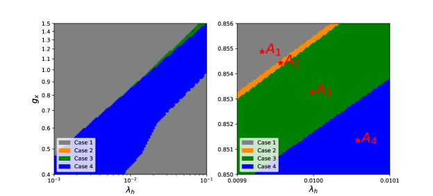
Figure 1: Left panel: The parameter space in the $\lambda_{h}$-$g_{x}$ plane divided into four regions with distinct colors, each corresponding to a different phase transition case for the cases (Case 1 -Case 4) discussed in section (2.2) where Case 2 occupies a region too small to be visible. Right panel: A magnified view of a small region of the left panel is displayed. Here four characteristic points labeled $A_{1}-A_{4}$ defined in Fig. (2) are marked on the plot.

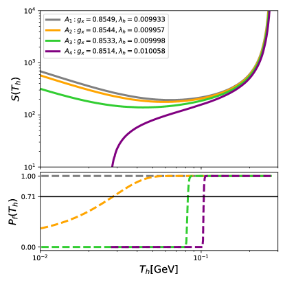
Figure 2: The bounce action $S(T_{h})$ (solid lines) and percolation probability $P_{f}(T_{h})$ (dashed lines) are plotted vs $T_{h}$ for four characteristic points labeled $A_{1}-A_{4}$ defined by $g_{x}$ and $\lambda_{h}$.

The left panel of Fig. 1 shows the parameter space spanning $\lambda_{h}\in(10^{-3},2\times 10^{-1})$ versus $g_{x}\in(0.4,1.5)$, with the right panel showing the region $\lambda_{h}\in(0.0099,0.0101)$ versus $g_{x}\in(0.850,0.856)$. The space is partitioned into four distinct regions, each colored differently to represent different types of phase transitions, which are:

Case 1: Here first-order phase transitions do not occur. There are two such regions in the left panel of Fig. 1. The first one is the upper dark region and is called the “ultracooled” region, where the potential barrier becomes too large for the transition to achieve percolation. The second one is the lower dark “crossover” region, where the transition from the false vacuum to the true vacuum is smooth and continuous, with no barriers between phases, thus precluding a first-order phase transition. The supercooled first-order phase transition of interest lies on the boundary of the “ultracooled” region.

Case 2: Here first-order phase transitions either do not complete or the physical volume of the false vacuum does not decrease at $T_{h,p}$. In this case, while percolation is successfully achieved with $P_{f}=0.71$, the phase transition either fails to complete ($P_{f}\nless 0.01$ at the end) or the physical volume of the false vacuum $V_{false}\propto a^{3}(t)P_{f}(t)$ increases due to a growing scale factor $a(t)$ via Hubble expansion, preventing bubble collisions and thus gravitational wave generation. Traditionally, the constraint on a decreasing volume of the false vacuum is satisfied by [18, 49]:

$$\frac{\beta_{*}}{H_{*}}>3.$$ (2.16)

However, since using $\beta_{*}$ for a supercooled phase transition leads to a significant error, an alternative constraint is employed [47, 4]:

$$3+\left.T_{h,p}\frac{d\mathcal{V}_{t}^{ext}}{dT_{h}}\right|_{T_{h}=T_{h,p}}<0,$$ (2.17)

where $-\mathcal{V}_{t}^{ext}$ is the exponent in Eq.  (2.12).

Case 3: The first-order phase transition successfully completes with a permanent potential barrier (i.e., the barrier persists even at $T_{h}=0$). A typical feature of this case is that the action curve $S(T)$ has a U-shape. With such a U-shape, we can achieve a small transition rate since $\frac{dS(T_{h})}{dT_{h}}$ can approach zero. This case is expected to have a sufficiently small transition rate with strong enough transition strength to fit PTA signals.

Case 4: The first-order phase transition successfully completes with the metastable false vacuum disappearing at some non-zero temperature. A typical feature of this case is that the action curve $S(T)$ has a “tangent-like” shape. In this case, the transition rate is generally large because the action curve is a monotonically increasing function, meaning $\frac{dS(T_{h})}{dT_{h}}$ is typically large. This case is expected to exhibit either a weak supercooled phase transition or a non-supercooled phase transition.

Four model model points labeled $A_{i}$ ($i=1,2,3,4$) one for each of the Cases 1-Case 4 are shown in Fig. 2 where the bounce action $S$ and the percolation probability $P_{f}$ versus $T_{h}$ are plotted in Fig. 2 to illustrate each case. For $A_{1}$, the percolation probability $P_{f}(T_{h})$ is a straight horizontal line equal to 1, indicating that percolation never occurs. For $A_{2}$, the transition is so slow that $P_{f}$ takes considerable time to decrease from 1 to 0, and consequently, we find the physical volume of the false vacuum increasing at the percolation temperature. For $A_{3}$, the transition is fast and generates gravitational waves . In this case, we observe a U-shaped action curve. For $A_{4}$, the false vacuum disappears in finite time, ensuring the completion of the transition. It exhibits a typical “tangent-like” action curve characteristic of weakly supercooled or non-supercooled phase transitions. From the right panel of Fig. 1, we find that by decreasing $g_{x}$ or increasing $\lambda_{h}$, phase transitions progress from Case 1 to Case 4. Case 3 is of particular interest because it generates gravitational waves strong enough to fit PTA signals. From the left panel of Fig. 1, we observe that Case 3 occupies a larger area as $\lambda_{h}$ increases, indicating that a strongly supercooled phase transition favors a larger $\lambda_{h}$. Conversely, when $\lambda_{h}$ is very small, Case 3 may disappear entirely, which suggests that a supercooled phase transition is prohibited.

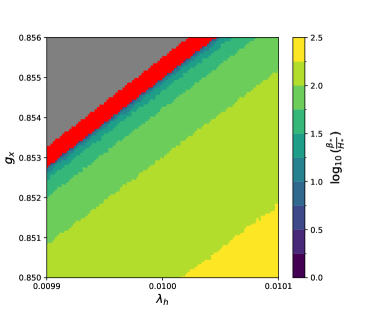
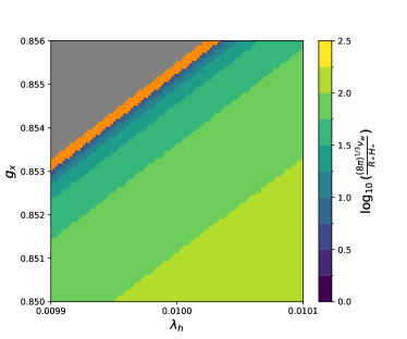
Figure 3: Left panel: An display of $log_{10}(\beta_{*}/H_{*})$ given by Eq.(2.14) in the $\lambda_{h}$-$g_{x}$ plane. The gray region represents Case 1. The red region shows the constraint given by $\beta_{*}/H_{*}>3$. The remaining region shows a color map of $\beta_{*}/H_{*}$ values. Right panel: The gray and orange regions represent Case 1 and Case 2, respectively. The remaining region shows a color map of $\frac{(8\pi)^{1/3}v_{w}}{R_{*}H_{*}}$ by Eq.(2.15).

To demonstrate the significant error introduced by the approximation in Eq. (2.10), we analyze two terms: $\beta_{*}/H_{*}$ and $\frac{(8\pi)^{1/3}v_{w}}{R_{*}H_{*}}$. These terms should have comparable values if the approximation holds. In Fig. 3, we present two color maps of these terms within the parameter space $\lambda_{h}\in(0.0099,0.0101)$ versus $g_{x}\in(0.850,0.856)$, which correspond to the zoomed-in region shown in Fig. 1. In the plots of Fig. 3, the gray and the orange regions indicate Case 1 and Case 2, respectively. The red region represents the constraint imposed by $\beta_{*}/H_{*}>3$, which is commonly considered when using $\beta_{*}/H_{*}$. The color maps of the left panel and the right panel of Fig. 3 exhibit stark differences, clearly demonstrating that the approximation in Eq. (2.10) fails when analyzing supercooled phase transitions. Further, we observe that for given values of $\lambda_{h}$ and $g_{x}$, $\beta_{*}/H_{*}$ consistently yields larger values than $\frac{(8\pi)^{1/3}v_{w}}{R_{*}H_{*}}$, indicating that using $\beta_{*}/H_{*}$ leads to an underestimation of the final gravitational wave power spectrum. Notably, the red region substantially exceeds the orange region, suggesting that applying Eq. (2.16) incorrectly excludes physically viable parameters. These parameters lie near the boundary of the “ultracooled” region, indicating that strongly supercooled phase transitions can arise in this region that can potentially generate gravitational wave power spectrum powerful enough to match PTA signals.

3 Why thermal history is important for a supercooled phase transition

The temperature ratio $\xi$ between the hidden and the visible sectors, enters in hidden sector phase transitions, as discussed in several previous studies [33, 24, 50, 38, 43]. The effective number of relativistic species, $N_{\rm eff}$ and the transition strength, $\alpha_{\rm tot}$, are two factors that are significantly influenced by the temperature ratio $\xi$. Generally, there are two types of transition strength parameters, as discussed in [24, 50]:

$$\alpha_{\rm tot} =\frac{\Delta\bar{\theta}(T_{h,p})}{\rho_{\rm rad}^{v}(T_{v,p})+\rho_{\rm rad}^{h}(T_{h,p})},$$ (3.1)

$$\alpha_{h} =\frac{\Delta\bar{\theta}(T_{h,p})}{\rho_{\rm rad}^{h}(T_{h,p})},$$ (3.2)

where $T_{h,p}$ and $T_{v,p}$ are the percolation temperatures in the hidden and visible sectors, respectively. Below we show that $\alpha_{tot}$ which controls the gravitational wave power spectrum is proportional to $\xi_{p}$ where $\xi_{p}=T_{h,p}/T_{v,p}$ indicating the strong role that $\xi$ plays in generating gravitational waves strong enough to match the PTA signal. In Eq.(3.2), $\Delta\bar{\theta}$ represents the amount of vacuum energy released during the transition [51, 52], and is defined as:

$$\Delta\bar{\theta}(T_{h}) =\bar{\theta}_{f}(T_{h})-\bar{\theta}_{t}(T_{h}),$$ (3.3)

$$\bar{\theta}_{i}(T_{h}) =\frac{1}{4}\left(\rho^{h}_{i}-\frac{p^{h}_{i}(T_{h})}{c_{s,t}^{2}(T_{h})}\right),$$ (3.4)

where

$$p^{h}_{i}(\phi_{i},T_{h}) =\frac{\pi^{2}}{90}g^{h}_{eff}(T_{h})T_{h}^{4}-V^{h}_{eff}(\phi_{i},T_{h}),$$ (3.5)

$$\rho^{h}_{i}(\phi_{i},T_{h}) =T_{h}\frac{\partial p^{h}_{i}}{\partial T_{h}}-p^{h}_{i},$$ (3.6)

$$c^{2}_{s,t}(T_{h}) =\frac{\partial p^{h}_{t}}{\partial\rho^{h}_{t}}=\frac{\partial p^{h}_{t}/\partial T_{h}}{\partial\rho^{h}_{t}/\partial T_{h}},$$ (3.7)

Here the notation “$f$” and “$t$” stand for the false vacuum and the true vacuum. As noted above the parameter $\alpha_{tot}$ enters directly in the gravitational wave power spectrum analysis while $\alpha_{h}$ enters in hydrodynamic computations for the hidden sector to determine the efficiency factor $\kappa$ and the bubble wall velocity $v_{w}$ when the visible sector is either very weakly coupled to or decoupled from the hidden sector. However, if there is a strong coupling between the visible and hidden sectors, the situation can be quite different. In this work, we assume that the visible sector is weakly coupled to the hidden sector during the phase transition, so $\alpha_{h}$ is primarily used for energy budget calculations. In the case of a supercooled phase transition, we expect $\alpha_{h}\gg 1$. However, to measure the strength of the first-order phase transition and the gravitational waves it generates, $\alpha_{\rm tot}$ should be used instead.

In the class of models discussed here, we typically have $g_{\rm eff}^{v}\gg g_{\rm eff}^{h}$, where $g_{\rm eff}^{v}$ is the number of degrees of freedom in the visible sector and $g_{\rm eff}^{h}$ is the number of degrees of freedom in the hidden sector. In this case, we expect that the main contribution to the radiation energy density comes from the visible sector, where the radiation energy density is given by $\rho_{\rm rad,v}(T_{h})=\frac{\pi^{2}}{30}g_{\rm eff}^{v}\left(\frac{T_{h,p}}{\xi_{p}}\right)^{4}$. Consequently, we find that [33]

$$\alpha_{\rm tot} \sim\frac{\Delta\bar{\theta}(T_{h,p})}{\rho_{\rm rad}^{v}(T_{v,p})}\sim\frac{\Delta\bar{\theta}(T_{h,p})}{\frac{\pi^{2}}{30}g_{\rm eff}^{v}\left(\frac{T_{h,p}}{\xi_{p}}\right)^{4}}\propto\xi_{p}^{4},$$ (3.8)

which means it is possible to have $\alpha_{tot}\ll 1$ even for a strong supercooled phase transition with $\alpha_{h}\gg 1$. To generate observable signals in PTAs, it is desirable to maximize $\alpha_{\rm tot}$, which in turn means maximizing $\xi_{p}$. On the other hand, the effective number of additional neutrino species,

$$\Delta N_{\rm eff}=\frac{4}{7}g^{h}_{eff}(T_{h,BBN})\left(\frac{11}{4}\right)^{4/3}\xi_{BBN}^{4},$$ (3.9)

scales as $\xi_{BBN}^{4}$, and observations from BBN and CMB impose the constraint $\Delta N_{\rm eff}<0.3$ [53]. These two conditions, i.e., maximizing $\alpha_{\rm tot}$ and limiting $\Delta N_{\rm eff}$, are in conflict, which substantially constrains the viable parameter space for $\xi$.

This conflict becomes more pronounced for a supercooled phase transition when reheating becomes non-negligible. To find the reheating temperature $T_{h,reh}$, we assume that reheating completes instantaneously around the time of bubble percolation. Energy conservation (see Section 5) then gives us:

$$\rho^{h}_{rad}(T_{h,reh})\simeq\rho^{h}_{rad}(T_{h,p})+\rho^{h}_{vac}(T_{h,p})$$ (3.10)

For strong phase transitions, such as those which are of interest in this work, we have $\rho_{\rm vac}^{h}(T_{h})\simeq\Delta\bar{\theta}(T_{h})$. Combining Eqs. (3.10) and (3.2), we obtain:

$$T_{h,reh}=\left(1+\alpha_{h}\right)^{\frac{1}{4}}\left(\frac{g^{h}_{eff}(T_{h,p})}{g^{h}_{eff}(T_{h,reh})}\right)^{\frac{1}{4}}T_{h,p}$$ (3.11)

Solving this equation yields $T_{h,reh}$. Since reheating occurs so rapidly that all released heat is transferred to the hidden sector, the temperature of the visible sector remains unchanged:

$$T_{v,reh}=T_{v,p}$$ (3.12)

This leads to a new temperature ratio after reheating:

$$\xi_{reh}=\frac{T_{h,reh}}{T_{v,reh}}$$ (3.13)

In a supercooled phase transition, we know that $\alpha_{h}\gg 1$, which implies $T_{h,reh}\gg T_{h,p}$ and consequently $\xi_{reh}\gg\xi_{p}$. This exacerbates the conflict since we need $\xi_{reh}$ to be as small as possible to satisfy the BBN constraint on $\Delta N_{\rm eff}$, while simultaneously requiring $\xi_{p}$ to be as large as possible to generate gravitational waves strong enough to match PTA signals. A detailed analysis by [24] shows that for a stable hidden sector, the viable parameter space is severely restricted. However, as also noted in [24], a dark sector decaying at pre-BBN temperature could resolve this conflict. We will examine this scenario with a detailed analysis in the following subsection.

3.1 Thermal evolution of coupled hidden and visible sectors

Thermal evolution of the hidden and the visible sectors are affected by coupling between the two sectors. Such couplings can exist via a variety of portals which include kinetic mixing of gauge fields [54], via Higgs coupling to the visible and the hidden sectors [55] and via Stueckelberg mass mixing[56, 57, 58] among others. In this work, we assume kinetic mixing for convenience. We generally use the notation $T_{h}$ for the hidden sector temperature and $T_{v}$ for the visible sector temperature. To describe the synchronous evolution of the hidden and the visible sectors we define

$$T_{h}=\xi(T_{v})T_{v}$$ (3.14)

where $\xi(T_{v})$ is an evolution function that relates the visible and the hidden sector temperatures. It is also convenient to sometime use $\zeta(T_{h})$ where

$$T_{v}=\zeta(T_{h})T_{h}$$ (3.15)

which allows to fix the temperature in the visible sector given the temperature in the hidden sector. $\zeta(T_{h})$ and $\xi(T_{v})$ are simply related: $\zeta(T_{h})=\xi^{-1}(T_{v})$ and $\xi(T_{v})$ and $\zeta(T_{h})$ are alternately used as needed to simplify notation. To find $\xi(T_{v})$, we start from the coupled Boltzmann equations in an expanding universe so that

$$\frac{d\rho_{v}}{dt}+3H(\rho_{v}+p_{v})=j_{v},$$

$$\frac{d\rho_{h}}{dt}+3H(\rho_{h}+p_{h})=j_{h}.$$ (3.16)

Here $\rho_{v},p_{v}$ and $\rho_{h},p_{h}$ are the energy and pressure densities for the visible and hidden sectors, and where $j_{v},j_{h}$ encode in them all the possible processes exchanging energy between these sectors [59, 60]. The evolution equation for $\xi(T)$ is given by [61, 62, 63]

$$\frac{d\xi}{dT_{v}}=\left[-\xi\frac{d\rho_{h}}{dT_{h}}+\frac{4H\sigma_{h}\rho_{h}-j_{h}}{4H\sigma\rho-4H\sigma_{h}\rho_{h}+j_{h}}\frac{d\rho_{v}}{dT_{v}}\right](T\frac{d\rho_{h}}{dT_{h}})^{-1}.$$ (3.17)

where $\sigma=\frac{3}{4}(1+\frac{p_{v}+p_{h}}{\rho_{v}+\rho_{h}}),\sigma_{h}=\frac{3}{4}(1+\frac{p_{h}}{\rho_{h}})$. In the analysis using the above one needs to pay attention to the limit when $\rho_{h}\rightarrow 0$ which happens for the case of a decaying dark sector. To study the thermal evolution of a decaying hidden sector, we account for the energy density not only through thermal equilibrium analysis but also by including the contribution from the relic abundance. Details on this can be found in Appendix E of [43]. In Eq.(3.17) $j_{h}$ depends on the particle content and their interactions in the hidden sector, which can be gotten by solving the Boltzmann equations for the yields discussed below:

$$\frac{dY_{q}}{dT}= -\frac{\mathbb{\mathbb{s}}}{H}\left(\frac{d\rho_{v}/dT}{{4\sigma\rho-4\sigma_{h}\rho_{h}}+j_{h}/H}\right)\Big{[}\frac{1}{2}\left<\sigma v\right>_{q\bar{q}\rightarrow i\bar{i}}(T)(Y_{q}^{eq}(T)^{2}-Y_{q}^{2})$$

$$-\frac{1}{2}\left<\sigma v\right>_{q\bar{q}\rightarrow\gamma^{\prime}{\gamma^{\prime}}}(T_{h})\left(Y_{q}^{2}-Y_{q}^{eq}(T_{h})^{2}\frac{Y_{\gamma^{\prime}}^{2}}{Y_{\gamma^{\prime}}^{eq}(T_{h})^{2}}\right)\Big{]}\,,$$ (3.18)

$$\frac{dY_{\gamma^{\prime}}}{dT}= -\frac{\mathbb{\mathbb{s}}}{H}\left(\frac{d\rho_{v}/dT}{{4\sigma\rho-4\sigma_{h}\rho_{h}}+j_{h}/H}\right)\left[\frac{1}{2}\left<\sigma v\right>_{q\bar{q}\rightarrow\gamma^{\prime}{\gamma^{\prime}}}(T_{h})\left(Y_{q}^{2}-Y_{q}^{eq}(T_{h})^{2}\frac{Y_{\gamma^{\prime}}^{2}}{Y_{\gamma^{\prime}}^{eq}(T_{h})^{2}}\right)+\right.$$

$$\frac{1}{2}\left<\sigma v\right>_{\phi\bar{\phi}\rightarrow\gamma^{\prime}{\gamma^{\prime}}}(T_{h})\left(Y_{\phi}^{2}-Y_{\phi}^{eq}(T_{h})^{2}\frac{Y_{\gamma^{\prime}}^{2}}{Y_{\gamma^{\prime}}^{eq}(T_{h})^{2}}\right)+\left<\sigma v\right>_{i\bar{i}\rightarrow\gamma^{\prime}}(T)Y_{i}^{eq}(T)^{2}$$

$$\left.-\frac{1}{\mathbb{\mathbb{s}}}\left<\Gamma_{\gamma^{\prime}\rightarrow i\bar{i}}(T_{h})\right>Y_{\gamma^{\prime}}+\left<\Gamma_{\phi\rightarrow\gamma^{\prime}\gamma^{\prime}}(T_{h})\right>\left(Y_{\phi}-Y^{eq}_{\phi}(T_{h})\frac{Y_{\gamma^{\prime}}^{2}}{Y^{eq}_{\gamma^{\prime}}(T_{h})^{2}}\right)\right]\,,$$ (3.19)

$$\frac{dY_{\phi}}{dT}= -\frac{\mathbb{\mathbb{s}}}{H}\left(\frac{d\rho_{v}/dT}{{4\sigma\rho-4\sigma_{h}\rho_{h}}+j_{h}/H}\right)\big{[}-\frac{1}{2}\left<\sigma v\right>_{\phi\bar{\phi}\rightarrow\gamma^{\prime}{\gamma^{\prime}}}(T_{h})\left(Y_{\phi}^{2}-Y_{\phi}^{eq}(T_{h})^{2}\frac{Y_{\gamma^{\prime}}^{2}}{Y_{\gamma^{\prime}}^{eq}(T_{h})^{2}}\right)$$

$$-\frac{1}{\mathbb{\mathbb{s}}}\left<\Gamma_{\phi\rightarrow\gamma^{\prime}\gamma^{\prime}}(T_{h})\right>\left(Y_{\phi}-Y^{eq}_{\phi}(T_{h})\frac{Y_{\gamma^{\prime}}^{2}}{Y^{eq}_{\gamma^{\prime}}(T_{h})^{2}}\right)\big{]}\,.$$ (3.20)

In the set of equations above $\mathbb{\mathbb{s}}$ is the entropy density and $Y_{i}$ are the yields defined by $Y_{i}=n_{i}/\mathbb{\mathbb{s}}$ To solve the differential equation set, Eq. (3.17,3.18,3.19,3.20), we need to set up the initial values for $\xi$ and the yields $Y_{\gamma^{\prime}},Y_{q}$, and $Y_{\phi}$. For a freeze-in process the initial value of $\xi$ is labeled $\xi_{0}$ and is taken to be zero. More generally we will assume $\xi_{0}$ to be a free parameter. More details may be found in Section 2.2 of [43].

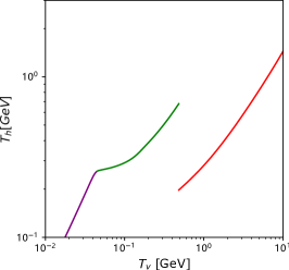
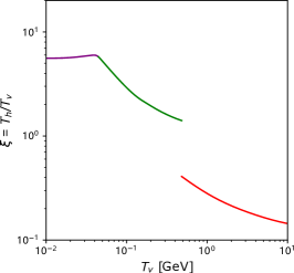
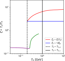
Figure 4: Temperature evolution of the hidden and visible sectors for benchmark point BP1 from Table 1. The evolution shows three distinct epochs: Phase 1 (red), before reheating; Phase 2 (green), after the reheating; and Phase 3 (purple), after the hidden sector particles decouple from each other. Left panel: Evolution of $T_{h}$ v.s. $T_{v}$. Middle panel: Evolution of $\xi$ v.s. $T_{v}$. Right panel: Evolution of $\zeta$ v.s. $T_{h}$. The vertical dashed line marks the point $T_{h}=T_{h,p}$ and the solid line marks the critical temperature for the hidden sector $T_{h}=T_{h,c}$. The blue line is the case $\zeta(T_{h})=1/\xi_{p}=\text{const}$.

The temperature evolution of the hidden and visible sectors for model BP1 is analyzed in Fig.(4). This evolution can be divided into three distinct epochs: Phase 1 (red), occurring before the phase transition and reheating; Phase 2 (green), following the phase transition and reheating; and Phase 3 (purple), when the hidden sector particles decouple from each other. During Phases 1 and 2, the evolution of $\xi(T_{v})$ is governed by Eq.(3.17). There is a discontinuous jump between Phase 1 and Phase 2, corresponding to the instantaneous reheating (analyzed in the previous section).

According to Table 1, for BP1 the lightest hidden sector particle (LHP) is $\phi$ with a mass of $1.28$ GeV. When the hidden sector temperature falls below this mass, the sector becomes non-relativistic, and its particles are expected to annihilate and decay into other particles. However, if the coupling between the hidden and visible sectors is very small (as is the case in this work), the radiational energy of the hidden sector converts into chemical potential rather than transferring to the visible sector, yielding the entropy density:

$$s_{h}\simeq\frac{m_{\phi}-\mu_{\phi}}{T_{h}}n_{\phi}.$$ (3.21)

If the hidden sector maintains efficient number-changing processes, such as $\phi\phi\phi\to\phi\phi$, the chemical potential vanishes ($\mu_{\phi}=0$) while preserving the hidden-sector entropy. In this scenario, the hidden sector effectively consumes its own particles to maintain its temperature, causing $\xi$ to increase continuously ($\zeta$ decreasing). This mechanism is known as ”cannibalism.” For detailed discussions of cannibalism and the associated phase transition, see Refs. [64, 34, 24, 32]. The cannibalism persists after the phase transition concludes, continuing into Phase 2. The process terminates when either the number-changing processes become inactive or the hidden sector loses thermal contact and particles decouple from each other. In the analysis of this work, the latter case stops the cannibalism—specifically, when the interaction rate between hidden sector particles becomes smaller than the Hubble parameter. At this point, the hidden sector particles freeze out, marking the transition to Phase 3.

During Phase 3, changes in the hidden sector temperature can occur only due to the universe’s expansion, similar to the visible sector. Consequently, the visible and the hidden sector temperatures evolve at the same rate, resulting in $\xi\sim\zeta\sim\text{const}$ during this phase. Once the cannibalism phase ends, the hidden sector becomes fully non-relativistic, causing $g^{h,rad}_{eff}$ to decrease exponentially. This leads $\Delta N_{eff}$ to rapidly approach zero, indicating that the hidden sector particles’ contribution to the radiation energy density becomes negligible. Consequently, the constraint on $\Delta N_{eff}$ is naturally satisfied. Meanwhile, the middle panel demonstrates that $\xi$ can reach $\mathcal{O}(1)$ at phase transition without violating the $\Delta N_{\rm eff}$ constraint. Thus, in the case of a decaying hidden sector, the apparent tension between $\alpha_{tot}$ and $\Delta N_{\rm eff}$ is resolved.

On the right panel, we indicate both $T_{h,p}$ and $T_{h,c}$ on the plot. The graph shows that the temperature ratio changes dramatically between $T_{h,c}$ and $T_{h,p}$. In most previous works in the literature, the temperature ratio was generally assumed to be constant, as indicated by the horizontal blue line. In the next section, we will demonstrate how $\zeta(T_{h})$ is involved in analyzing a hidden supercooled phase transition, highlighting the necessity of considering synchronous evolution hidden and visible sectors.

3.2 How thermal history of hidden and visible sectors enter in supercooled phase transitions

In section 2.2, we have discussed some details of supercooled phase transition when assuming $\xi(T_{v})=\zeta(T_{h})=1$. However, in most cases the temperature ratio varies significantly during and before the phase transition, especially for a decaying hidden sector, as discussed in the previous section. In this section, for a temperature dependent $\xi(T_{v})$ or $\zeta(T_{h})$, we will investigate how the analysis on supercooled phase transition could be modified. The percolation temperature, $T_{h,p}$, is defined as the point at which $71\%$ of the universe remains in the false vacuum, i.e.,

$$P_{f}(T_{h,p})=0.71$$ (3.22)

where

$$P_{f}(T_{h})=\exp\left(-\frac{4\pi}{3}v_{w}^{3}\int_{T_{h}}^{T_{h,c}}dT^{\prime}\frac{\Gamma(T_{h}^{\prime})}{T_{h}^{\prime}H^{4}(T_{h}^{\prime})}\left(\int_{T_{h}}^{T_{h}^{\prime}}dT_{h}^{\prime\prime}\frac{1}{H(T_{h}^{\prime\prime})}\right)^{3}\right)$$ (3.23)

The Hubble parameter $H(T_{h})$ is evaluated at the hidden sector temperature $T_{h}$:

$$H(T_{h})=\sqrt{\frac{8\pi G}{3}\rho_{tot}}=\sqrt{\frac{8\pi G}{3}\left(\rho^{v}_{rad}(\zeta(T_{h})T_{h})+\rho^{h}_{rad}(T_{h})+\rho^{h}_{vac}(T_{h})\right)},$$ (3.24)

where $G$ is Newton’s gravitational constant,

$$\rho^{v}_{rad}(T_{v}) =\frac{\pi}{30}g_{eff}^{v}(T_{v})T_{v}^{4},$$ (3.25)

$$\rho^{h}_{rad}(T_{h}) =\frac{\pi}{30}g_{eff}^{h}(T_{h})T_{h}^{4},$$ (3.26)

$$\rho^{h}_{vac}(T_{h}) \simeq\left.V_{\rm eff}^{h}(\phi,T_{h})-T_{h}\frac{\partial V^{h}_{\rm eff}}{\partial T_{h}}\right|_{\phi=\phi_{f}}-\rho^{h}_{gs},$$ (3.27)

and $\rho^{h}_{gs}$ in Eq.(3.24) is the zero-temperature ground state energy density, and ${V_{\rm eff}^{h}(\phi,T_{h})}$ is the effective potential for the hidden sector [47].

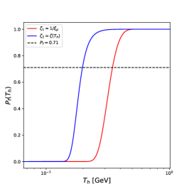
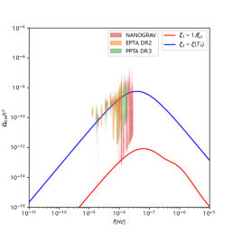
Figure 5: Illustration of the significant effect of thermal histories of the visible and the hidden sectors on the Hubble parameter, percolation temperature and the gravitational power spectrum through their dependence on the parameter $\zeta(T_{h})=T_{v}/T_{h}$. Left Panel: The Hubble parameter $H(T_{h})$ as a function of the hidden sector temperature $T_{h}$ versus $T_{h}$ for two different choices of $\zeta$ where $\zeta$ is defined by Eq.(3.15). The vertical dashed line marks the point the percolation temperature for the hidden sector $T_{h}=T_{h,p}$ and the solid line marks the critical temperature for the hidden sector $T_{h}=T_{h,c}$. Middle Panel: $P_{f}(T_{h})$ versus $T_{h}$ for two different choices of $\zeta$. The horizontal dashed line marks $P_{f}=0.71$. Right Panel: Gravitational wave power spectrum $\Omega_{GW}h^{2}$ for two different choices of $\zeta$. Colored areas represent PTA signals. Benchmark model BP1 from Table. 1 is applied for all three figures.

The synchronous evolution function, $\zeta(T_{h})$, appearing in Eq. (3.24), can modify the evolution history of the Hubble parameter and, consequently, affect the percolation temperature, since the Hubble parameter appears in the integral Eq. (3.23). For weakly supercooled or non-supercooled phase transitions, such effects are typically limited because $T_{h,p}/T_{h,c}\sim 1$, implying that the Hubble parameter does not change significantly during the small interval between $T_{h,p}$ and $T_{h,c}$. However, for strongly supercooled transitions, its influence becomes significant. To illustrate the Hubble parameter’s sensitivity to temperature ratio evolution, we consider two different scenarios: $\zeta_{1}=\text{const}=1/\xi_{p}$ and $\zeta_{2}=\zeta(T_{h})$. In the first scenario, the temperature is constant, which is commonly suggested in most works in the literature.

In the second scenario, we introduce an evolving temperature ratio. An important observation is that for these two scenarios, we have $\zeta_{2}=\zeta(T_{h,p})=1/\xi_{p}=\zeta_{1}$. Thus, for weakly supercooled or non-supercooled phase transitions, these two scenarios are identical. We then plot $H(T_{h})$ for these two scenarios on the left panel of Fig. 5 using the benchmark model BP1. Here, we use dashed and solid lines to mark $T_{h}=T_{h,p}$ and $T_{h}=T_{h,c}$, which are the upper and lower limits appearing in the Integral Eq. (3.23,2.15). The figure shows that at $T_{h}=T_{h,p}$, the Hubble parameter is the same for both scenarios as discussed, while it can differ by a factor of 10 at $T_{h}=T_{h,c}$. In the middle panel, we have $P_{f}(T_{h})$ versus $T_{h}$ for two different choices of $\zeta$. We observe a significant difference between these two cases, where the percolation temperatures differ by 100%. This substantial change in $T_{h,p}$ significantly affects other parameters, including $\alpha_{tot},H_{*}$ and $R_{*}$. The effect of the temperature dependence is even more drastic on the gravitational wave power spectrum. The right panel of Fig. 5 shows the gravitational wave power spectrum for the two different $\zeta$. We notice that they differ by a factor of as much as $10^{4}$, which would seriously impact fits to the PTA signals.

4 Computation of the gravitational wave power spectrum and fits to PTA data

We carry out the analysis in two parts. In the first part we will present a set of benchmark models and study the power spectrum in detail as a function of the frequency for the supercooled phase transition. Here we show that the gravitational wave power spectrum allows a fit to the PTA data in the range of frequencies observed by NANOGrav, EPTA and PPTA. In the second part we will present a Monte Carlo analysis relevant for the PTA signal. We discuss these below.

4.1 Benchmark models for PTA signal

We provide five benchmark points in Table 1 that generate sufficiently strong GWs to match the PTA signal while satisfying other cosmological constraints. The relevant parameters are listed in Table 2, and the resulting gravitational wave power spectrum is shown in Fig. 6.

	$m_{q}$	$g_{x}$	$f_{x}$	$\delta$($\times 10^{-12}$)	$\xi_{0}$	$\mu_{h}$	$\lambda_{h}$	$m_{A}$	$m_{\phi}$
(BP1)	28.69	2.147	1.53e-03	6.948	0.118	0.906	0.2805	3.67	1.28
(BP2)	32.28	2.824	1.38e-05	11.387	0.185	8.023	0.7706	25.81	11.35
(BP3)	8.43	2.105	2.53e-04	8.573	0.116	0.262	0.2601	1.08	0.37
(BP4)	31.41	2.378	1.20e-03	8.472	0.133	0.337	0.4055	1.26	0.48
(BP5)	25.67	0.821	9.15e-03	5.543	0.231	8.195	0.0086	72.64	11.59

Table 1: Benchmark points BP1-BP5 where the parameters $m_{q},g_{x},f_{x},\delta,\mu_{h},\lambda_{h}$ are defined as in Eq.(2.1) and Eq.(2.2) and $\xi_{0}$ is the initial temperature ratio between two sectors. All masses are in unit of GeV.

	$T_{h,p}$	$T_{h,reh}$	$T_{h,c}$	$T_{v,p}$	$\xi_{p}$	$\alpha_{tot}$	$\alpha_{h}$	$\frac{\beta_{*}}{H_{*}}$	$\frac{(8\pi)^{1/3}v_{w}}{H_{*}R_{*}}$	$\Omega_{DM}h^{2}$
(BP1)	0.197	0.679	1.017	0.483	0.408	0.298	1769	-308.89	4.05	0.039
(BP2)	1.592	4.500	6.934	1.979	0.804	1.509	1096	-261.70	4.05	0.109
(BP3)	0.050	0.200	0.299	0.138	0.362	0.979	6397	-375.37	3.86	0.049
(BP4)	0.066	0.228	0.341	0.154	0.425	0.789	2992	-331.40	3.91	0.050
(BP5)	2.969	13.66	23.415	5.966	0.498	2.790	2497	-29.01	6.38	0.014

Table 2: A display of the output of Table(1) for the benchmarks BP1-BP5. $T_{h,p}$ and $T_{v,p}$ are the percolation temperatures for the hidden and the visible sectors where $T_{h,reh}$ and $T_{h,c}$ are the reheat and the critical temperatures and $\xi_{p}$ is $\xi$ at the percolation temperature. Further, $\alpha_{tot}$ and $\alpha_{h}$ are defined by Eq.(3.1,3.2), $\beta_{*}/H_{*}$ is defined by Eq.(2.14), $R_{*}$ by Eq.(2.15) and $\Omega_{DM}h^{2}$ is the dark matter relic density. All temperatures are in unit of GeV.

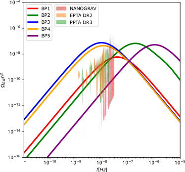
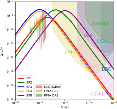
Figure 6: Left Panel: The gravitational power spectrum $\Omega_{GW}h^{2}$ for supercooled phase transitions as a function of the frequency $f$ in the range [$10^{-11}-10^{-5}$] [Hz] for five benchmark points BP1-BP5. Colored areas represent PTA signals, given by NANOGrav [3], PPTA [1], and EPTA [2]. Right Panel: Detection regions from future space-based GW detectors are shown, including LISA [65, 66, 67], BBO[68], Decigo[69], Taiji[70], TianQin[71], and $\mu$Ares[72]. The right panel shows that supercooled phase transitions also can produce detectable signals in the higher frequency regions above NanoGrav.

In Table 2, we list the signature temperatures, including the critical temperature $T_{h,c}$, reheating temperature $T_{h,reh}$, and percolation temperature $T_{h,p}$ in the hidden sector. We also provide the visible sector percolation temperature $T_{v,p}$, which is used when calculating the redshift. We observe that the temperature ratio during the phase transition, $\xi_{p}$, is generally large, which enables a strong phase transition, with $\alpha_{tot}\sim\mathcal{O}(1)$. For all benchmark points, the hidden sector becomes non-relativistic before BBN, thereby satisfying $\Delta N_{\rm eff}$ constraints. Our calculations of $\frac{\beta_{*}}{H_{*}}$ and $\frac{(8\pi)^{1/3}v_{w}}{H_{*}R_{*}}$ reveal that $\frac{\beta_{*}}{H_{*}}$ is negative for these benchmark points. While this would have excluded them under the previous constraint $\beta_{*}/H_{*}>3$, these points are now valid since we employ the mean bubble separation $R_{*}$ instead. In the final column, we present the total relic density contributed by $\phi$ and $q$, calculated by solving the Boltzmann equations Eq. (3.17,3.18,3.19,3.20). These results demonstrate that our model can account for at least a portion of the dark matter content. Fig. 6 displays the calculated gravitational wave power spectra for all benchmark points. These spectra not only reach but in some cases exceed the observed PTA signal, providing strong potential for future observations. The right panel also illustrates the detection regions of future space-based gravitational wave detectors, including LISA, BBO, Decigo, Taiji, TianQin, and $\mu$Ares. The power spectra from our benchmark points fall within these detection regions, suggesting that the model discussed here can be tested by these detectors in the future.

4.2 Contribution to the GW Signal

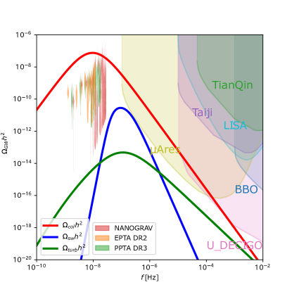
Figure 7: The three primary contributions to the GW signal for BP3: bubble collisions (red), sound waves in the plasma (blue), and turbulence in the plasma (green). The analysis indicates that the dominant contribution to the gravitational waves comes from bubble collisions while the contributions from sound waves and turbulence are essentially negligible in the nano-Hz region.

There are three primary contributions to the GW signal: bubble collisions, sound waves in the plasma, and turbulence in the plasma. If a true vacuum bubble generated during the phase transition continues to accelerate to a velocity close to the speed of light ($v_{w}\simeq 1$), this is referred to as the runaway scenario. In this case, most of the energy is stored in the bubble walls, and GWs are predominantly generated by bubble collisions. Conversely, if the bubble reaches a terminal velocity $v_{w}<1$, it is termed the non-runaway scenario. Here, most of the energy resides in the plasma, and GWs are primarily produced by sound waves and turbulence. The distinction between the runaway and non-runaway scenarios depends on whether the friction exerted by the plasma is comparable to the pressure difference driving the bubble expansion [73]. A detailed analysis of this is provided in Appendix 7.1.

For all BPs, we generally find that $\alpha_{h,\infty}<\alpha_{h}$, indicating that they all correspond to runaway scenarios. As shown in Fig. 7, the dominant contribution to the GW signal comes from bubble collisions.

4.3 Monte Carlo analysis of model points covering the PTA signal

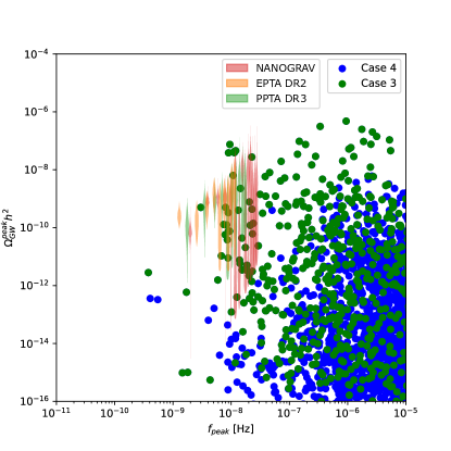
Figure 8: Results of Monte Carlo analysis showing gravitational power spectrum peaks for two different supercooled phase transition scenarios: Case 3 and Case 4. Green points represent Case 3 and blue points are for Case 4. All points shown satisfy the cosmological constraint on $\Delta N_{\text{eff}}$ and dark matter relic density requirement ($0.001<\Omega_{\text{DM}}h^{2}<0.12$). The sampling was performed along the boundary of the ultracooled region with small fluctuations.

Fig. 8 presents the result of a Monte Carlo analysis performed on 7 free parameters: $m_{q}$,$g_{x}$,$f_{x}$, $\delta$, $\xi_{0}$, $\mu_{h}$, $\lambda_{h}$. To conserve computational resources, we conducted the Monte Carlo sampling along the boundary of the “ultracooled” region with small fluctuations. Each point in the figure represents the peak of a gravitational wave power spectrum curve. All displayed points correspond to successfully completed phase transitions that satisfy both the cosmological constraint on $\Delta N_{eff}$ and the dark matter relic density requirement ($0.001<\Omega_{DM}h^{2}<0.12$). The points are color-coded, with green and blue points corresponding to Case 3 and Case 4, respectively, as discussed in section 2.2. The results demonstrate that numerous Case 3 models readily achieve PTA signal levels. In contrast, virtually none of the Case 4 models reach PTA signal levels while simultaneously satisfying all the cosmological constraints.

5 Gravitational Wave Energy Density in PTA signal region

In this section we discuss the energy transfer to gravitational waves during the phase transition. An approximation of the energy density ratio is given by [12]:

$$\frac{\rho_{GW}}{\rho_{tot}}\sim\kappa^{2}\left(\frac{\alpha}{1+\alpha}\right)\left(\frac{\beta}{H}\right)^{-2}.$$ (5.1)

However, as discussed in Section 2.2, $\beta$ may not be an appropriate parameter to describe the transition rate of a supercooled phase transition. Here we compute the energy density ratio numerically. The gravitational wave power spectrum before redshift is defined as:

$$\Omega_{GW}=\frac{1}{\rho_{tot}}\frac{\partial\rho_{GW}}{\partial\ln{f}}$$ (5.2)

With $\Omega_{GW}$ given in Section 7, we can determine the ratio:

$$\frac{\rho_{GW}}{\rho_{tot}}=\frac{\int d\rho_{GW}}{\rho_{tot}}=\int_{-\infty}^{\infty}\frac{\Omega_{GW}}{f}df.$$ (5.3)

Furthermore, we have $\alpha_{tot}\simeq\frac{\rho_{vac}}{\rho_{tot}}$. Using these relations, we can calculate $\frac{\rho_{GW}}{\rho_{vac}}$.

No.	$\frac{\rho_{GW}}{\rho_{tot}}$(units:$10^{-3}$)	$\alpha_{tot}\simeq\frac{\rho_{vac}}{\rho_{tot}}$	$\frac{\rho_{GW}}{\rho_{vac}}$(units:$10^{-3}$)
BP1	0.31	0.30	1.10
BP2	3.30	1.51	2.18
BP3	2.83	0.98	2.89
BP4	1.73	0.79	2.19
BP5	2.39	2.79	0.85

Table 3: Energy density ratios for different benchmark points (BP1-BP5) of Table (1). The table gives the ratio of the gravitational wave energy density to the total energy density ($\frac{\rho_{GW}}{\rho_{tot}}$), the approximate ratio of the vacuum energy density to the total energy density ($\alpha_{tot}$), and the resulting ratio of the gravitational wave energy density to the vacuum energy density ($\frac{\rho_{GW}}{\rho_{vac}}$).

Table 3 presents the ratios for five benchmark points given in Table 1. As shown, for all the benchmark points shown, only about (0.1-0.3)% of the vacuum energy is transferred to the gravitational wave energy. Thus, the energy conservation assumption expressed in Eq.(3.10) remains valid.

6 Conclusion

In this paper, we explored the possibility that the nano-Hertz gravitational wave signal observed by the recent PTA experiments arise from a supercooled first-order phase transition within a hidden sector featuring a spontaneously broken $U(1)_{X}$ gauge symmetry. We emphasize in our analysis the use of mean bubble separation $R_{*}$, rather than the inverse timescale $\beta_{*}$, in characterizing supercooled phase transitions. In Fig. 3, we demonstrated how naively adopting $\beta_{*}/H_{*}$ for strongly supercooled scenarios can lead to substantial errors. Here we show that a large portion of the parameter space that would otherwise appear excluded by the commonly used condition $\beta_{*}/H_{*}>3$ is in fact viable once $R_{*}$ is used in place of $\beta$.

In addition, the main new feature of our analysis over existing works is that we have taken into account thermal histories of coupled hidden and visible sectors evolving their temperature ratio $\xi(T_{v})$ or alternately $\zeta(T_{h})$ in a synchronous fashion. We highlight in Fig. 5 that a nontrivial evolution of $\zeta(T_{h})$ can significantly affect the Hubble parameter during the transition (see the left panel of Fig.(5)), thereby modifying the percolation temperature $T_{h,p}$ and the mean bubble separation $R_{*}$. In particular, the longer integration range between $T_{h,c}$ and $T_{h,p}$ in a supercooled scenario amplifies the impact of how $\xi$ and $\zeta$ evolve. The sensitivity to $\xi$ is also reflected in the percolation temperature as exhibited in the middle panel of Fig.(5). Further, ignoring the $\xi$ evolution can lead to discrepancies of up to four orders of magnitude in the predicted gravitational wave power spectrum as exhibited the right panel of Fig.(5). The results of our analysis are illustrated through several benchmark points, each of which satisfies important cosmological and astrophysical constraints and gives an observable gravitational wave power spectrum. We presented these spectra in Fig. 6 and demonstrated that hidden sector FOPTs can generate gravitational waves in the PTA frequency range with sufficient power to match current observations. Further, some benchmark models predict signals within the reach of future gravitational wave experiments such as LISA, Taiji, and others.

In summary, our study shows that with a more complete analysis which properly takes into account the subtleties discussed in this work, the supercooled hidden sector phase transitions can naturally generate gravitational wave backgrounds that explain the current PTA data. We have provided a systematic treatment of the supercool phase transitions and demonstrated that both the mean bubble separation $R_{*}$ and the synchronous temperature ratio $\xi(T_{v})$ and $\zeta(T_{h})$ play crucial roles in the gravitational wave power spectrum analysis. Consequently, the analysis presented here offers a robust framework for further investigation of the cosmic first order phase transitions and for further exploration of their role in the analysis of stochastic gravitational wave backgrounds in $[10^{-9}-10^{-2}]$Hz frequency range with levels of power spectrum accessible to current and future gravitational wave detectors.

Acknowledgments
The research was supported in part by the NSF Grant PHY-2209903.

7 Appendix: Details of GW Power Spectrum

A number of factors enter in the gravitational wave power spectrum and have been discussed in depth in the literature. We give here a brief summary of some of the elements that enter prominently in the analysis. Thus gravitational wave power spectrum involves the hydrodynamics of the bubble nucleation includes the efficiency factor $\kappa$ and the bubble wall velocity $v_{w}$. Further, the gravitational wave power spectrum receives contributions from bubble collision, from sound waves and from turbulence. We discuss these further below.

7.1 Hydrodynamics, Efficiency Factor and Bubble Wall Velocity

In the main text of the paper, we have discussed many aspects of the supercooled phase transition in a hidden $U(1)_{X}$ model, including temperatures $T_{h,p}$ and $T_{h,reh}$, transition strengths $\alpha_{tot}$ and $\alpha_{h}$, and transition rates $\frac{\beta_{*}}{H_{*}}$ and $\frac{1}{H_{*}R_{*}}$. In the analysis of gravitational waves  generated by a first-order phase transition (FOPT), there are two remaining parameters to consider, which enter in the hydrodynamics of bubble expansion: the efficiency factor $\kappa$ and bubble wall velocity $v_{w}$ [74, 75, 52, 51, 76, 77]. Here, the transition coefficient $\kappa(c_{s,f}^{2},c_{s,t}^{2},\alpha,v_{w})$ is calculated using $\alpha_{h}$ rather than $\alpha_{tot}$. Detailed calculations of $\kappa$ can be found in [51, 52], and we utilize their provided Python code for numerical calculations. The kinetic energy fraction is then given by

$$K=\frac{\Delta\bar{\theta}(T_{h,p})}{\rho_{tot}}\kappa(c_{s,f}^{2},c_{s,t}^{2},\alpha_{h},v_{w})\simeq\frac{\alpha_{tot}}{1+\alpha_{tot}}\kappa(c_{s,f}^{2},c_{s,t}^{2},\alpha_{h},v_{w})$$ (7.1)

To determine the bubble wall velocity, we must first classify whether the bubble expansion is runaway or non-runaway [73]. This classification is made using a critical phase transition strength $\alpha_{h,\infty}$, defined as:

$$\alpha_{h,\infty}=\frac{(T_{h,p})^{2}}{\rho^{h}_{\rm rad}(T_{h,p})}\left(\sum_{i=\text{bosons}}n_{i}\frac{\Delta m_{i}^{2}}{24}+\sum_{i=\text{fermions}}n_{i}\frac{\Delta m_{i}^{2}}{48}\right)$$ (7.2)

In the runaway regime, where $\alpha_{h,\infty}<\alpha_{h}$, we have:

$$\kappa_{\phi}=1-\frac{\alpha_{\infty}}{\alpha_{h}},\quad\kappa_{\rm sw}=\frac{\alpha_{\infty}}{\alpha_{h}}\kappa(\alpha_{\infty},c^{2}_{s,f},c^{2}_{s,t},v_{w}),\quad v_{w}=1$$ (7.3)

Conversely, in the non-runaway regime, where $\alpha_{h,\infty}>\alpha_{h}$, we have:

$$\kappa_{\phi}=0,\quad\kappa_{\rm sw}=\kappa(\alpha_{h},c^{2}_{s,f},c^{2}_{s,t},v_{w})$$ (7.4)

For the non-runaway case, $v_{w}$ requires further determination. Following the method described in [78, 77], we calculate $v_{w}(\alpha_{h},c_{s,f}^{2},c_{s,t}^{2},\Phi_{p})$, where:

$$\Phi_{p}=\frac{w_{t}(\phi_{t},T_{h,p})}{w_{f}(\phi_{f},T_{h,p})},\quad w^{h}_{i}(\phi_{i},T_{h})=p^{h}_{i}(\phi_{i},T_{h})+\rho^{h}_{i}(\phi_{i},T_{h})$$ (7.5)

with $p^{h}_{i}$ and $\rho^{h}_{i}$ given in Eqs. (3.5, 3.6). Our analysis shows that for any supercooled phase transition events capable of producing a PTA signal, the $\alpha_{h}$ is generally too large to yield deflagration or hybrid solutions. Thus all PTA events end up as detonation type with

$$v_{w}\approx v_{J}=c_{s,f}\left(\frac{1+\sqrt{3\alpha_{h}(1+c_{s,f}^{2}(3\alpha_{h}-1))}}{1+3\alpha_{h}c_{s,f}^{2}}\right),$$ (7.6)

where $v_{J}$ is the Chapman-Jouguet velocity. Thus, taking $v_{w}=v_{J}$ serves as a reasonable approximation, at least within the context of the hidden $U(1)_{X}$ model under investigation.

7.2 Details of the gravitational power spectrum

Gravitational waves produced during the early universe undergo redshifting. To correctly match the gravitational waves we observe today with those produced during the early universe, we need to consider this effect. For a hidden sector phase transition, the power spectrum $\Omega^{0}_{GW}(f_{0})$ at the current temperature $T_{v,0}$ from the power spectrum $\Omega_{GW}$ obtained at the temperature $T_{v,reh}$ is given by

$$\Omega^{0}_{GW}(f_{0}) =\mathcal{R}_{\Omega}\Omega_{GW}\left(\frac{1}{\mathcal{R}_{f}}f_{0}\right),~~\frac{1}{\mathcal{R}_{f}}=\frac{a_{0}}{a}=\left(\frac{h_{eff}(T_{v,reh})}{h^{0}_{eff}}\right)^{1/3}\left(\frac{T_{v,reh}}{T_{v}^{0}}\right)$$

$$\mathcal{R}_{\Omega} \equiv\left(\frac{a}{a_{0}}\right)^{4}\left(\frac{H}{H_{0}}\right)^{2}\simeq 2.473\times 10^{-5}h^{-2}\left(\frac{h^{0}_{eff}}{h_{eff}(T_{v,reh})}\right)^{4/3}\left(\frac{g_{eff}(T_{v,reh})}{2}\right)$$

$$g_{eff}(T_{v,reh}) =g_{eff}^{v}(T_{v,reh})+g_{eff}^{h}(T_{v,reh})\xi(T_{v,reh})^{4}$$

$$h_{eff}(T_{v,reh}) =h_{eff}^{v}(T_{v,reh})+h_{eff}^{h}(T_{v,reh})\xi(T_{v,reh})^{3}$$

$$h^{0}_{eff} \simeq 3.91$$

where $T_{v}^{0}=2.35\times 10^{-13}$GeV is today’s temperature. Since the reheating occurs within the hidden sector, the visible sector temperature remains unaffected. Consequently, the final GW power spectrum is not significantly impacted even in the presence of strong reheating, unlike the case discussed in [4]. The computations of the gravitational wave power spectrum have been carried out by a number of authors  [79, 80, 81, 82, 83, 8, 84, 85, 73, 86]. These results are collected in Appendix E of [4] which we utlize in the analysis of this work. The gravitational wave power spectrum includes contributions from bubble collision, from sound waves, and from turbulence. Their relative contributions are discussed in detail in Fig. (7) where one finds that the PTA signal is dominated by the gravitational wave arising from bubble collision.

References

- [1] D. J. Reardon, A. Zic, R. M. Shannon, G. B. Hobbs, M. Bailes, V. Di Marco, A. Kapur, A. F. Rogers, E. Thrane and J. Askew, et al. Astrophys. J. Lett. 951, no.1, L6 (2023) doi:10.3847/2041-8213/acdd02 [arXiv:2306.16215 [astro-ph.HE]].
- [2] J. Antoniadis et al. [EPTA and InPTA:], Astron. Astrophys. 678, A50 (2023) doi:10.1051/0004-6361/202346844 [arXiv:2306.16214 [astro-ph.HE]].
- [3] G. Agazie et al. [NANOGrav], Astrophys. J. Lett. 951, no.1, L8 (2023) doi:10.3847/2041-8213/acdac6 [arXiv:2306.16213 [astro-ph.HE]].
- [4] P. Athron, A. Fowlie, C. T. Lu, L. Morris, L. Wu, Y. Wu and Z. Xu, Phys. Rev. Lett. 132, no.22, 221001 (2024) doi:10.1103/PhysRevLett.132.221001 [arXiv:2306.17239 [hep-ph]].
- [5] K. Kawana, Phys. Rev. D 105, no.10, 103515 (2022) doi:10.1103/PhysRevD.105.103515 [arXiv:2201.00560 [hep-ph]].
- [6] M. Lewicki and V. Vaskonen, Eur. Phys. J. C 83, no.2, 109 (2023) doi:10.1140/epjc/s10052-023-11241-3 [arXiv:2208.11697 [astro-ph.CO]].
- [7] S. W. Hawking and I. G. Moss, Phys. Lett. B 110, 35-38 (1982) doi:10.1016/0370-2693(82)90946-7
- [8] T. Ghosh, A. Ghoshal, H. K. Guo, F. Hajkarim, S. F. King, K. Sinha, X. Wang and G. White, JCAP 05, 100 (2024) doi:10.1088/1475-7516/2024/05/100 [arXiv:2307.02259 [astro-ph.HE]].
- [9] P. Athron, L. Morris and Z. Xu, JCAP 05, 075 (2024) doi:10.1088/1475-7516/2024/05/075 [arXiv:2309.05474 [hep-ph]].
- [10] E. Madge, E. Morgante, C. Puchades-Ibáñez, N. Ramberg, W. Ratzinger, S. Schenk and P. Schwaller, JHEP 10, 171 (2023) doi:10.1007/JHEP10(2023)171 [arXiv:2306.14856 [hep-ph]].
- [11] K. Fujikura, S. Girmohanta, Y. Nakai and M. Suzuki, Phys. Lett. B 846, 138203 (2023) doi:10.1016/j.physletb.2023.138203 [arXiv:2306.17086 [hep-ph]].
- [12] P. Athron, C. Balázs, A. Fowlie, L. Morris and L. Wu, Prog. Part. Nucl. Phys. 135, 104094 (2024) doi:10.1016/j.ppnp.2023.104094 [arXiv:2305.02357 [hep-ph]].
- [13] L. Sagunski, P. Schicho and D. Schmitt, Phys. Rev. D 107, no.12, 123512 (2023) doi:10.1103/PhysRevD.107.123512 [arXiv:2303.02450 [hep-ph]].
- [14] Y. Nakai, M. Suzuki, F. Takahashi and M. Yamada, Phys. Lett. B 816, 136238 (2021) doi:10.1016/j.physletb.2021.136238 [arXiv:2009.09754 [astro-ph.CO]].
- [15] J. Ellis, M. Lewicki and V. Vaskonen, JCAP 11, 020 (2020) doi:10.1088/1475-7516/2020/11/020 [arXiv:2007.15586 [astro-ph.CO]].
- [16] A. Kobakhidze, C. Lagger, A. Manning and J. Yue, Eur. Phys. J. C 77, no.8, 570 (2017) doi:10.1140/epjc/s10052-017-5132-y [arXiv:1703.06552 [hep-ph]].
- [17] Y. Gouttenoire and T. Volansky, Phys. Rev. D 110, no.4, 043514 (2024) doi:10.1103/PhysRevD.110.043514 [arXiv:2305.04942 [hep-ph]].
- [18] K. Freese and M. W. Winkler, Phys. Rev. D 106, no.10, 103523 (2022) doi:10.1103/PhysRevD.106.103523 [arXiv:2208.03330 [astro-ph.CO]].
- [19] M. Fairbairn, E. Hardy and A. Wickens, JHEP 07, 044 (2019) doi:10.1007/JHEP07(2019)044 [arXiv:1901.11038 [hep-ph]].
- [20] X. Wang, F. P. Huang and X. Zhang, JCAP 05, 045 (2020) doi:10.1088/1475-7516/2020/05/045 [arXiv:2003.08892 [hep-ph]].
- [21] A. Megevand and S. Ramirez, Nucl. Phys. B 919, 74-109 (2017) doi:10.1016/j.nuclphysb.2017.03.009 [arXiv:1611.05853 [astro-ph.CO]].
- [22] L. Leitao and A. Megevand, JCAP 05, 037 (2016) doi:10.1088/1475-7516/2016/05/037 [arXiv:1512.08962 [astro-ph.CO]].
- [23] J. Ellis, M. Lewicki, J. M. No and V. Vaskonen, JCAP 06, 024 (2019) doi:10.1088/1475-7516/2019/06/024 [arXiv:1903.09642 [hep-ph]].
- [24] T. Bringmann, P. F. Depta, T. Konstandin, K. Schmidt-Hoberg and C. Tasillo, JCAP 11, 053 (2023) doi:10.1088/1475-7516/2023/11/053 [arXiv:2306.09411 [astro-ph.CO]].
- [25] Z. Arzoumanian et al. [NANOGrav], Astrophys. J. Lett. 905, no.2, L34 (2020) doi:10.3847/2041-8213/abd401 [arXiv:2009.04496 [astro-ph.HE]].
- [26] B. Goncharov, R. M. Shannon, D. J. Reardon, G. Hobbs, A. Zic, M. Bailes, M. Curylo, S. Dai, M. Kerr and M. E. Lower, et al. Astrophys. J. Lett. 917, no.2, L19 (2021) doi:10.3847/2041-8213/ac17f4 [arXiv:2107.12112 [astro-ph.HE]].
- [27] S. Chen et al. [EPTA], Mon. Not. Roy. Astron. Soc. 508, no.4, 4970-4993 (2021) doi:10.1093/mnras/stab2833 [arXiv:2110.13184 [astro-ph.HE]].
- [28] S. Blasi, V. Brdar and K. Schmitz, Phys. Rev. Lett. 126, no.4, 041305 (2021) doi:10.1103/PhysRevLett.126.041305 [arXiv:2009.06607 [astro-ph.CO]].
- [29] M. Benetti, L. L. Graef and S. Vagnozzi, Phys. Rev. D 105, no.4, 043520 (2022) doi:10.1103/PhysRevD.105.043520 [arXiv:2111.04758 [astro-ph.CO]].
- [30] V. Vaskonen and H. Veermäe, Phys. Rev. Lett. 126, no.5, 051303 (2021) doi:10.1103/PhysRevLett.126.051303 [arXiv:2009.07832 [astro-ph.CO]].
- [31] W. Buchmuller, V. Domcke and K. Schmitz, Phys. Lett. B 811, 135914 (2020) doi:10.1016/j.physletb.2020.135914 [arXiv:2009.10649 [astro-ph.CO]].
- [32] T. Bringmann, T. E. Gonzalo, F. Kahlhoefer, J. Matuszak and C. Tasillo, JCAP 05, 065 (2024) doi:10.1088/1475-7516/2024/05/065 [arXiv:2311.06346 [astro-ph.CO]].
- [33] M. Breitbach, J. Kopp, E. Madge, T. Opferkuch and P. Schwaller, JCAP 07, 007 (2019) doi:10.1088/1475-7516/2019/07/007 [arXiv:1811.11175 [hep-ph]].
- [34] F. Ertas, F. Kahlhoefer and C. Tasillo, JCAP 02, no.02, 014 (2022) doi:10.1088/1475-7516/2022/02/014 [arXiv:2109.06208 [astro-ph.CO]].
- [35] A. Banik, Y. Cui, Y. D. Tsai and Y. Tsai, [arXiv:2412.16282 [hep-ph]].
- [36] J. Jaeckel, V. V. Khoze and M. Spannowsky, Phys. Rev. D 94, no.10, 103519 (2016) doi:10.1103/PhysRevD.94.103519 [arXiv:1602.03901 [hep-ph]].
- [37] P. Schwaller, Phys. Rev. Lett. 115, no.18, 181101 (2015) doi:10.1103/PhysRevLett.115.181101 [arXiv:1504.07263 [hep-ph]].
- [38] S. P. Li and K. P. Xie, Phys. Rev. D 108, no.5, 055018 (2023) doi:10.1103/PhysRevD.108.055018 [arXiv:2307.01086 [hep-ph]].
- [39] P. Di Bari, D. Marfatia and Y. L. Zhou, JHEP 10, 193 (2021) doi:10.1007/JHEP10(2021)193 [arXiv:2106.00025 [hep-ph]].
- [40] Z. Chen, K. Ye and M. Zhang, Phys. Rev. D 107, no.9, 095027 (2023) doi:10.1103/PhysRevD.107.095027 [arXiv:2303.11820 [hep-ph]].
- [41] S. Kanemura and S. P. Li, JCAP 03, 005 (2024) doi:10.1088/1475-7516/2024/03/005 [arXiv:2308.16390 [hep-ph]].
- [42] R. H. Cyburt, B. D. Fields, K. A. Olive and T. H. Yeh, Rev. Mod. Phys. 88, 015004 (2016) doi:10.1103/RevModPhys.88.015004 [arXiv:1505.01076 [astro-ph.CO]].
- [43] W. Z. Feng, J. Li and P. Nath, Phys. Rev. D 110, no.1, 015020 (2024) doi:10.1103/PhysRevD.110.015020 [arXiv:2403.09558 [hep-ph]].
- [44] J. Löfgren, M. J. Ramsey-Musolf, P. Schicho and T. V. I. Tenkanen, Phys. Rev. Lett. 130, no.25, 251801 (2023) doi:10.1103/PhysRevLett.130.251801 [arXiv:2112.05472 [hep-ph]].
- [45] K. Enqvist, J. Ignatius, K. Kajantie and K. Rummukainen, Phys. Rev. D 45, 3415-3428 (1992) doi:10.1103/PhysRevD.45.3415
- [46] C. Caprini, M. Chala, G. C. Dorsch, M. Hindmarsh, S. J. Huber, T. Konstandin, J. Kozaczuk, G. Nardini, J. M. No and K. Rummukainen, et al. JCAP 03, 024 (2020) doi:10.1088/1475-7516/2020/03/024 [arXiv:1910.13125 [astro-ph.CO]].
- [47] P. Athron, C. Balázs and L. Morris, JCAP 03, 006 (2023) doi:10.1088/1475-7516/2023/03/006 [arXiv:2212.07559 [hep-ph]].
- [48] C. L. Wainwright, Comput. Phys. Commun. 183, 2006-2013 (2012) doi:10.1016/j.cpc.2012.04.004 [arXiv:1109.4189 [hep-ph]].
- [49] M. S. Turner, E. J. Weinberg and L. M. Widrow, Phys. Rev. D 46, 2384-2403 (1992) doi:10.1103/PhysRevD.46.2384
- [50] Y. Bai and M. Korwar, Phys. Rev. D 105, no.9, 095015 (2022) doi:10.1103/PhysRevD.105.095015 [arXiv:2109.14765 [hep-ph]].
- [51] F. Giese, T. Konstandin, K. Schmitz and J. van de Vis, JCAP 01, 072 (2021) doi:10.1088/1475-7516/2021/01/072 [arXiv:2010.09744 [astro-ph.CO]].
- [52] F. Giese, T. Konstandin and J. van de Vis, JCAP 07, no.07, 057 (2020) doi:10.1088/1475-7516/2020/07/057 [arXiv:2004.06995 [astro-ph.CO]].
- [53] N. Aghanim et al. [Planck], Astron. Astrophys. 641, A6 (2020) [erratum: Astron. Astrophys. 652, C4 (2021)] doi:10.1051/0004-6361/201833910 [arXiv:1807.06209 [astro-ph.CO]].
- [54] B. Holdom, Phys. Lett. B 166, 196-198 (1986) doi:10.1016/0370-2693(86)91377-8
- [55] B. Patt and F. Wilczek, [arXiv:hep-ph/0605188 [hep-ph]].
- [56] B. Kors and P. Nath, Phys. Lett. B 586, 366-372 (2004) doi:10.1016/j.physletb.2004.02.051 [arXiv:hep-ph/0402047 [hep-ph]].
- [57] D. Feldman, Z. Liu and P. Nath, Phys. Rev. D 75, 115001 (2007) doi:10.1103/PhysRevD.75.115001 [arXiv:hep-ph/0702123 [hep-ph]].
- [58] M. Du, Z. Liu and P. Nath, Phys. Lett. B 834, 137454 (2022) doi:10.1016/j.physletb.2022.137454 [arXiv:2204.09024 [hep-ph]].
- [59] A. Aboubrahim, W. Z. Feng, P. Nath and Z. Y. Wang, JHEP 06, 086 (2021) doi:10.1007/JHEP06(2021)086 [arXiv:2103.15769 [hep-ph]].
- [60] A. Aboubrahim and P. Nath, JHEP 09, 084 (2022) doi:10.1007/JHEP09(2022)084 [arXiv:2205.07316 [hep-ph]].
- [61] A. Aboubrahim, W. Z. Feng, P. Nath and Z. Y. Wang, Phys. Rev. D 103, no.7, 075014 (2021) doi:10.1103/PhysRevD.103.075014 [arXiv:2008.00529 [hep-ph]].
- [62] J. Li and P. Nath, Phys. Rev. D 108, no.11, 115008 (2023) doi:10.1103/PhysRevD.108.115008 [arXiv:2304.08454 [hep-ph]].
- [63] P. Nath and J. Li, LHEP 2024, 502 (2024) doi:10.31526/lhep.2024.502 [arXiv:2402.04123 [hep-ph]].
- [64] M. Farina, D. Pappadopulo, J. T. Ruderman and G. Trevisan, JHEP 12, 039 (2016) doi:10.1007/JHEP12(2016)039 [arXiv:1607.03108 [hep-ph]].
- [65] P. Amaro-Seoane et al. [LISA], [arXiv:1702.00786 [astro-ph.IM]].
- [66] J. Baker, J. Bellovary, P. L. Bender, E. Berti, R. Caldwell, J. Camp, J. W. Conklin, N. Cornish, C. Cutler and R. DeRosa, et al. [arXiv:1907.06482 [astro-ph.IM]].
- [67] P. Amaro-Seoane, S. Aoudia, S. Babak, P. Binetruy, E. Berti, A. Bohe, C. Caprini, M. Colpi, N. J. Cornish and K. Danzmann, et al. GW Notes 6, 4-110 (2013) [arXiv:1201.3621 [astro-ph.CO]].
- [68] C. Grojean and G. Servant, Phys. Rev. D 75, 043507 (2007) doi:10.1103/PhysRevD.75.043507 [arXiv:hep-ph/0607107 [hep-ph]].
- [69] S. Kawamura, T. Nakamura, M. Ando, N. Seto, K. Tsubono, K. Numata, R. Takahashi, S. Nagano, T. Ishikawa and M. Musha, et al. Class. Quant. Grav. 23, S125-S132 (2006) doi:10.1088/0264-9381/23/8/S17
- [70] W. H. Ruan, Z. K. Guo, R. G. Cai and Y. Z. Zhang, Int. J. Mod. Phys. A 35, no.17, 2050075 (2020) doi:10.1142/S0217751X2050075X [arXiv:1807.09495 [gr-qc]].
- [71] J. Luo et al. [TianQin], Class. Quant. Grav. 33, no.3, 035010 (2016) doi:10.1088/0264-9381/33/3/035010 [arXiv:1512.02076 [astro-ph.IM]].
- [72] A. Sesana, N. Korsakova, M. A. Sedda, V. Baibhav, E. Barausse, S. Barke, E. Berti, M. Bonetti, P. R. Capelo and C. Caprini, et al. Exper. Astron. 51, no.3, 1333-1383 (2021) doi:10.1007/s10686-021-09709-9 [arXiv:1908.11391 [astro-ph.IM]].
- [73] C. Caprini, M. Hindmarsh, S. Huber, T. Konstandin, J. Kozaczuk, G. Nardini, J. M. No, A. Petiteau, P. Schwaller and G. Servant, et al. JCAP 04, 001 (2016) doi:10.1088/1475-7516/2016/04/001 [arXiv:1512.06239 [astro-ph.CO]].
- [74] D. Bodeker and G. D. Moore, JCAP 05, 025 (2017) doi:10.1088/1475-7516/2017/05/025 [arXiv:1703.08215 [hep-ph]].
- [75] J. R. Espinosa, T. Konstandin, J. M. No and G. Servant, JCAP 06, 028 (2010) doi:10.1088/1475-7516/2010/06/028 [arXiv:1004.4187 [hep-ph]].
- [76] W. Y. Ai, B. Garbrecht and C. Tamarit, JCAP 03, no.03, 015 (2022) doi:10.1088/1475-7516/2022/03/015 [arXiv:2109.13710 [hep-ph]].
- [77] W. Y. Ai, B. Laurent and J. van de Vis, [arXiv:2411.13641 [hep-ph]].
- [78] W. Y. Ai, B. Laurent and J. van de Vis, JCAP 07, 002 (2023) doi:10.1088/1475-7516/2023/07/002 [arXiv:2303.10171 [astro-ph.CO]].
- [79] M. Hindmarsh, Phys. Rev. Lett. 120, no.7, 071301 (2018) doi:10.1103/PhysRevLett.120.071301 [arXiv:1608.04735 [astro-ph.CO]].
- [80] M. Hindmarsh and M. Hijazi, JCAP 12, 062 (2019) doi:10.1088/1475-7516/2019/12/062 [arXiv:1909.10040 [astro-ph.CO]].
- [81] C. Gowling, M. Hindmarsh, D. C. Hooper and J. Torrado, JCAP 04, 061 (2023) doi:10.1088/1475-7516/2023/04/061 [arXiv:2209.13551 [astro-ph.CO]].
- [82] M. Hindmarsh, S. J. Huber, K. Rummukainen and D. J. Weir, Phys. Rev. D 96, no.10, 103520 (2017) [erratum: Phys. Rev. D 101, no.8, 089902 (2020)] doi:10.1103/PhysRevD.96.103520 [arXiv:1704.05871 [astro-ph.CO]].
- [83] R. G. Cai, S. J. Wang and Z. Y. Yuwen, Phys. Rev. D 108, no.2, L021502 (2023) doi:10.1103/PhysRevD.108.L021502 [arXiv:2305.00074 [gr-qc]].
- [84] C. Caprini, R. Durrer and X. Siemens, Phys. Rev. D 82, 063511 (2010) doi:10.1103/PhysRevD.82.063511 [arXiv:1007.1218 [astro-ph.CO]].
- [85] C. Caprini, R. Durrer and G. Servant, JCAP 12, 024 (2009) doi:10.1088/1475-7516/2009/12/024 [arXiv:0909.0622 [astro-ph.CO]].
- [86] D. J. Weir, Phil. Trans. Roy. Soc. Lond. A 376, no.2114, 20170126 (2018) [erratum: Phil. Trans. Roy. Soc. Lond. A 381, 20230212 (2023)] doi:10.1098/rsta.2017.0126 [arXiv:1705.01783 [hep-ph]].