Private Minimum Hellinger Distance Estimation via Hellinger Distance Differential Privacy

Abstract

Hellinger distance has been widely used to derive objective functions that are alternatives to maximum likelihood methods. Motivated by recent regulatory privacy requirements, estimators satisfying differential privacy constraints are being derived. In this paper, we describe different notions of privacy using divergences and establish that Hellinger distance minimizes the added variance within the class of power divergences for an additive Gaussian mechanism. We demonstrate that a new definition of privacy, namely Hellinger differential privacy, shares several features of the standard notion of differential privacy while allowing for sharper inference. Using these properties, we develop private versions of gradient descent and Newton-Raphson algorithms for obtaining private minimum Hellinger distance estimators, which are robust and first-order efficient. Using numerical experiments, we illustrate the finite sample performance and verify that they retain their robustness properties under gross-error contamination.

Key words: Differential privacy, $\epsilon-$HDP, $(\lambda,\epsilon)-$PDP, adaptive composition, sequential composition, parallel composition, group privacy, PMHDE, private gradient descent, private Newton-Raphson, first-order efficiency, utility, robustness.

1 Introduction

Recently, the adoption of AI (artificial intelligence)- whose success relies on data- by many scientific fields has brought an increased focus on data privacy. Many entities collect individually identifiable data to provide personalized services and share them with other organizations to improve and enhance the quality of the service. However, such data-sharing activities lead to increased data privacy concerns. Specifically, in healthcare, data are often shared with various research groups to facilitate treatment payment operations and improve the quality of care. The Health Insurance Portability and Accountability Act (HIPAA), The Health Information Technology for Economic and Clinical Health (HITECH), the California Consumer Privacy Act (CCPA), and the General Data Protection Regulation (GDPR) are some of the recent regulations that impact commerce. Historically, anonymization techniques, like encrypting or removing personally identifiable information, have been widely used to ensure privacy protection. However, recent studies (Gymrek et al., 2013; Homer et al., 2008; Narayanan and Shmatikov, 2008; Sweeney, 1997) have shown that many of the existing anonymization methods are fragile and can lead to the leakage of private information. Specifically, an intruder might still be able to identify individuals by cross-classifying categorical variables in the dataset and matching them with some external database. A need for a rigorous technical framework to measure and analyze the de-identification methods has long been noted (see Duncan and Lambert (1986)).

Differential privacy (DP) is a probabilistic framework that quantifies how individual privacy is preserved in a database when certain information is released by querying the database. The basic idea behind the DP framework is to measure the indistinguishability, using a parameter $\epsilon$, of two probability distributions of a dataset in the presence or absence of a record. Small values of $\epsilon$ correspond to hard distinguishability and high privacy. The distributions in question typically correspond to those of statistics obtained by querying the database.

In an interactive setting of the DP, a data warehouse provides a group of query functions that allow users to pose queries about the data and receive responses with noise added for privacy (referred to as a mechanism). In a non-interactive setting, the data warehouses offer a dataset with added noise, and users can apply any models and methods to this data. Controlling privacy breaches is challenging in the non-interactive setting (see Dwork et al. (2006), for instance). In contrast, privacy-preserving mechanisms that rely on specific query functions without direct access to the dataset enable assessment of privacy and utility. In this paper, we focus on the interactive approach and assume the existence of a trusted curator holding individuals’ data in a database. The goal of private inference is to protect individual data while simultaneously allowing statistical analysis of the entire database. An analyst can only access a model’s perturbed summary statistics or outputs in such cases. While adding noise preserves privacy, the amount of noise needs to be small to ensure optimal statistical performance.

This paper describes a new notion, namely Hellinger distance differential privacy (HDP)- a particular case of power divergence privacy (PDP)- and studies private estimation and inference for Minimum Hellinger Distance Estimators (MHDEs). The power divergence family parameterized by $\lambda$ encompasses Rényi divergence up to a Logarithmic transformation. The classical $\epsilon-$ DP can be obtained by taking the limit as $\lambda$ diverges to infinity in the PDP. Following the privacy literature, we describe privacy using the parameters $\lambda$ and $\epsilon$ and the terminology $(\lambda,\epsilon)-$ PDP. When $\lambda=-\frac{1}{2}$, the power divergence reduces to twice the squared Hellinger distance between densities, and hence $(-\frac{1}{2},2\epsilon)-$ PDP is referred to as $\epsilon-$ HDP.

Some well-known differential privacy methods, such as $\epsilon-$ DP, $(\epsilon,\delta)-$ DP, and $(\alpha,\epsilon)-$ Rényi differential privacy (RDP) (Mironov (2017)) can be defined using statistical divergence measures and are subsumed in our $(\lambda,\epsilon)-$PDP. Specifically, for $\lambda>0$, $(\lambda,\epsilon)-$ PDP is equivalent to $(\lambda+1,\frac{1}{\lambda}\log(\epsilon\lambda(\lambda+1)+1)-$RDP. The parameter $\lambda$ in power divergence plays a similar role as $\alpha$ in Rényi divergence, for example $\lambda\in[1,2]$ corresponds to $\alpha\in[2,3]$. While the RDP focuses on the case $\lambda>0$, the case $\lambda<0$ has several useful properties. Specifically, it turns out that the additive Gaussian mechanism has minimal variance when $\lambda=-\frac{1}{2}$. This observation motivates a detailed study of this case, namely, the HDP. We establish that HDP has better composition and group privacy properties than RDP (see Theorem 2.3 and Theorem 2.4). We also discuss the relationship between HDP and other privacy frameworks, which broadens the potential applications of HDP.

Another contribution of our paper is the application of private optimization algorithms to obtain private MHDE (PMHDE). Previous studies on private optimization algorithms (Avella-Medina (2021); Chaudhuri et al. (2011); Chaudhuri and Hsu (2012); Chen et al. (2019); Dalenius (1977); Slavkovic and Molinari (2012); Wang et al. (2017)) have focused on M-estimators, which typically involves bounded score functions and convex loss functions. While M-estimators are well-known for their robustness, they are not statistically first-order efficient due to the boundedness of the score function. In contrast, MHDE achieves both robustness and first-order efficiency. This paper develops asymptotic properties of PMHDE obtained through private optimization algorithms without explicit assumptions of convexity and boundedness. While $\epsilon-$ HDP is used for privacy guarantees, the methods also work for any $(\lambda,\epsilon)-$ PDP, in particular, for $(\alpha,\epsilon)-$ RDP. Additionally, other approaches such as $\mu-$ GDP (Dong et al. (2022)) and $\rho-$ zCDP (Bun and Steinke (2016); Dwork and Rothblum (2016)) can also be used for privacy guarantees. Some of these are described in Section 2.

The sensitivity of the query function plays a central role in DP investigations. In applications in point estimation, the query concerns the gradient of the loss function under appropriate model regularity. Since the second-order properties of estimators also rely on the first and second-order derivatives of the loss functions, it is reasonable to anticipate a link between the sensitivity and statistical efficiency. We make this precise in Sections 3.4 and 3.5. Specifically, we obtain sharp estimates of the sensitivities of the gradient and Hessian of the Hellinger loss functions (see Theorem 3.1) and use them to derive the limit distribution of the PMHDE. The arguments required for establishing this are subtle and involved. Finally, it is worth emphasizing here that we do not make convexity assumptions. instead, we leverage the family regularity and the properties of the Hellinger objective function to develop our results.

Algorithms such as gradient descent (GD) and Newton-Raphson (NR) are typically used to obtain MHDE and other M-estimators (Avella-Medina et al. (2023); Bassily et al. (2014); Feldman et al. (2020); Lee and Kifer (2018); Song et al. (2013)). The private versions of these estimators are derived by optimizing the private objective functions that are obtained by adding an appropriate noise at every iteration. We study private versions of GD and NR, namely PGD and PNR, that output $\epsilon-$ HDP counterparts of MHDE, namely PMHDE (see Section 3.3). Analysis of these algorithms is critical to study the properties of the PMHDE. These are investigated in Section 3.4 and Section 3.5. We begin in Section 2 with the background and notations of DP, while in Section 4, we present several numerical experiments that evaluate the performance of our estimators under the true model and contamination. Section 5 contains some extensions and concluding remarks. The proofs of the main results are in Section 6. Several additional calculations needed for the paper are relegated to Appendices A through E.

2 Background, notations, and Hellinger distance differential privacy

Let $\{X_{n}:n\geq 1\}$ denote a collection of independent and identically distributed (i.i.d.) real-valued random variables defined on the probability space $(\Omega,\mathscr{F},P)$ and set $\mathbf{X}=(X_{1},X_{2},\cdots X_{n})$ so that $\mathbf{X}:(\Omega,\mathscr{F},P)\mapsto(\mathbb{R}^{n},\mathscr{B}(\mathbb{R}^{n}),P_{X})$, where $P_{X}$ is the induced probability measure on the Borel subsets of $\mathbb{R}^{n}$. We denote by $\mathscr{D}\subset\mathbb{R}^{n}$, the database of the i.i.d. observations; that is, $\mathscr{D}=\{\mathbf{X}(\omega):\omega\in\Omega\}$. A query function $W(\cdot)$ is a statistic; namely a measurable mapping $W:(\mathscr{D},\mathscr{B}(\mathbb{R}^{n}))\mapsto(\mathbb{R}^{m},\mathscr{B}(\mathbb{R}^{m}))$. We denote a typical element of $\mathscr{D}$, namely the dataset, by $D$, and the query applied to $D$ by $w\coloneqq W(D)$. In our applications, We will be interested in functions of the type, $f(w,D)$, where $f(\cdot,\cdot)$ is a measurable mapping from $(\mathbb{R}^{m}\times\mathbb{R}^{n},\mathscr{B}(\mathbb{R}^{m})\times\mathscr{B}(\mathbb{R}^{n}))\mapsto(\mathbb{R}^{m},\mathscr{B}(\mathbb{R}^{m}))$. A simple example of $f(w,D)$ is $f(w,D)=w$.

Next, we introduce one of the essential concepts of DP, namely the mechanism (or a randomized algorithm) denoted by $M$. In statistical terms, $M$ is a measurable mapping from $(\mathbb{R}^{m}\times\mathbb{R}^{n},\mathscr{B}(\mathbb{R}^{m})\times\mathscr{B}(\mathbb{R}^{n}))\mapsto(\mathbb{R}^{m},\mathscr{B}(\mathbb{R}^{m}))$. $M$ is said to be an additive mechanism, if $M(w,D)=f(w,D)+\mathbf{Y}$, where $\mathbf{Y}=[Y_{1},\cdots,Y_{m}]\in\mathbb{R}^{m}$, is a random vector (with i.i.d. components) representing the noise and independent of $(w,D)$. In here, $M(\cdot,\cdot)$ represents a private version of $f(\cdot,\cdot)$. Continuing with the above example, the additive mechanism will output $w+\mathbf{Y}$, a perturbed version of $w$.

A critical component of the privacy measure is the sensitivity of the query function. Formally, in DP, it is based on two adjacent datasets differing in one observation. Specifically, for $D,D^{\prime}\in\mathscr{D}$, set $z_{i}=\mathbbm{1}_{[x_{i}=x_{i}^{^{\prime}}]}$, for $1\leq i\leq n$. Then, the Hamming distance between $D$ and $D^{\prime}$ is given by

$$||D-D^{\prime}||_{H}=\sum_{i=1}^{n}z_{i}.$$

We say $D$ and $D^{\prime}$ are adjacent if $||D-D^{\prime}||_{H}=1$. Define ${L}_{1}$ and ${L}_{2}$ sensitivity of a query function $W$ to be

$$\Delta_{L_{1}}W=\sup\limits_{||D-D^{\prime}||_{H}=1}||W(D)-W(D^{\prime})||_{1}$$

$$\Delta_{L_{2}}W=\sup\limits_{||D-D^{\prime}||_{H}=1}||W(D)-W(D^{\prime})||_{2}.$$

We now turn to a precise description of some widely used DP measures. To this end, let $Q$ denote the conditional distribution of $M(w,D)$ given $w,D)$. We start with $\epsilon-$ differential privacy introduced in Dwork et al. (2006).

Definition 2.1.

A mechanism, ${M}$, satisfies $\epsilon-$ differential privacy (DP) if for any $S\in\mathscr{B}(\mathbb{R}^{m})$ and adjacent $D,D^{\prime}$,

$${}Q(M(w,D)\in S)\leq e^{\epsilon}\cdot Q(M(w,D^{\prime})\in S).$$ (2.1)

When $M$ is an additive mechanism, that is, $M(w,D)=W(D)+\mathbf{Y}$ and the random variables $Y_{1},Y_{2},\cdots,Y_{m}$ are i.i.d. with $Y_{1}\sim Lap(0,\frac{\Delta_{L_{1}}W}{\epsilon})$, then $M$ satisfies $\epsilon-$ DP. A natural case of an additive mechanism, namely the Gaussian mechanism, does not satisfy (2.1). Hence, a relaxation of $\epsilon-$(DP) was studied in Dwork et al. (2006) and is referred to as approximate DP or, more commonly, as $(\epsilon,\delta)-$DP.

Definition 2.2.

A mechanism $M$, satisfies $(\epsilon,\delta)-$ differential privacy (DP) if for any possible output $S\subset\mathscr{B}(\mathbb{R}^{m})$ and adjacent $D,D^{\prime}$,

$$Q(M(w,D)\in S)\leq e^{\epsilon}\cdot Q(M(w,D^{\prime})\in S)+\delta.$$

In this case, the distribution of $\mathbf{Y}$ is $N_{m}(\mathbf{0},\sigma^{2}\mathbf{I}_{m\times m})$, where

$$\sigma^{2}=\frac{2\cdot(\Delta_{L_{2}}W)^{2}\cdot\log(1.25/\delta)}{\epsilon^{2}}.$$

Other notions of relaxations of differential privacy have been studied in the literature. Some of the most commonly studied ones include concentrated differential privacy (CDP) (Dwork and Rothblum (2016)), zero concentrated differential privacy (zCDP) (Bun and Steinke (2016)), Gaussian differential privacy (Dong et al. (2022)), and Renyi differential privacy (RDP) (Mironov (2017)). Some of these approaches can be unified under the general notion of divergence. We first turn to the notion of Hellinger distance differential privacy (HDP) and a related generalization. In the following, for two random variables $X$ and $Y$ with distribution $P_{1}$ and $P_{2}$ respectively, we denote the divergence between them as $D(X,Y)$, which is equivalent to $D(P_{1},P_{2})$.

Definition 2.3.

(Hellinger differential privacy) A mechanism $M$ is said to satisfy $\epsilon-$ Hellinger differential privacy (HDP), if for any adjacent $D,D^{\prime}\in\mathscr{D}$,

$$D_{HD}(M(w,D),M(w,D^{\prime}))\leq\epsilon.$$

where for two distributions $P_{1},P_{2}$, with densities $p_{1}(\cdot)$ and $p_{2}(\cdot)$ with respect to (w.r.t.) the Lebesgue measure,

$$D_{HD}(P_{1},P_{2})=\int_{\mathbb{R}^{m}}\left(\sqrt{p_{1}(x)}-\sqrt{p_{2}(x)}\right)^{2}\mathrm{d}x.$$

By definition $\epsilon\in[0,2]$.

Hellinger distance is a member of the general class of divergences referred to as Power divergence, introduced by Cressie and Read (1984) and further analyzed in Read and Cressie (1988) for performing goodness of fit tests in multinomial and multivariate discrete data. The ideas were unified in the work of Lindsay (Lindsay (1994)), who studied general divergences for robust and efficient estimation in parametric models (see also Basu et al. (2011)). Let $P_{1}$ and $P_{2}$ be two probability distributions possessing densities $p_{1}(\cdot)$ and $p_{2}(\cdot)$ on $\mathbb{R}^{m}$. The power divergence $D_{\lambda}(P_{1},P_{2})$ between $P_{1}$ and $P_{2}$, denoted by $D_{\lambda}(P_{1},P_{2})$ is defined as follows: for $\lambda\neq-1,0$

$$D_{\lambda}(P_{1},P_{2})=\frac{1}{\lambda(\lambda+1)}\mathbf{E}_{X\sim p_{2}}\left[\left(\frac{p_{1}(X)}{p_{2}(X)}\right)^{\lambda+1}-1\right],$$

$D_{0}(P_{1},P_{2})$ and $D_{-1}(P_{1},P_{2})$ are defined by taking the limits as $\lambda$ approaches $0$ or $-1$. A standard calculation shows that

$$D_{0}(P_{1},P_{2})=D_{-1}(P_{2},P_{1})=KL(P_{1},P_{2}),$$

where $KL(\cdot,\cdot)$ represents the Kullback-Leibler divergence. Rényi divergence is a particular case of power divergence when $\lambda>0$; specifically, setting $\alpha=(\lambda+1)$, the Rényi divergence of order $\alpha$ is given by

$$D_{\alpha}^{(R)}(P_{1},P_{2})=\frac{1}{\lambda}\log\left[\lambda(\lambda+1)D_{\lambda}(P_{1},P_{2})+1\right].$$

When $P_{1}$ and $P_{2}$ have the same support, the limit of $D_{\lambda}(P_{1},P_{2})$ exists and is referred to as the Max divergence and is given by

$$D_{\infty}(P_{1},P_{2})\coloneqq\lim\limits_{\lambda\to\infty}\frac{1}{\lambda}\log[\lambda(\lambda+1)D_{\lambda}(P_{1},P_{2})+1]=\max_{S\in Supp(P_{1})}\log\frac{P_{1}(S)}{P_{2}(S)}.$$

A $\delta-$ ($0<\delta<1$) relaxation of the above Max divergence is given by

$$D_{\infty}^{\delta}(P_{1},P_{2})\coloneqq\max_{S\in Supp(P_{1}):P_{1}(S)\geq\delta}\log\frac{P_{1}(S)-\delta}{P_{2}(S)}.$$

Using the above notions, one can express the $\epsilon-$ DP, $(\epsilon,\delta)-$ DP, and $(\epsilon,\alpha)-$ RDP as follows: Let $D,D^{\prime}$ be adjacent. A mechanism, $M$ is $\epsilon-$DP if $D_{\infty}(M(W(D)),M(W(D^{\prime})))\leq\epsilon$, while it is $(\epsilon,\delta)-$DP if $D_{\infty}^{\delta}(M(W(D)),M(W(D^{\prime})))\leq\epsilon$. It is said to be $(\alpha,\epsilon)-$RDP ($\alpha>1$) if $D_{\alpha}^{(R)}(M(W(D)),M(W(D^{\prime})))\leq\epsilon$. We now turn to describe a new privacy measure called Power Divergence Differential Privacy (PDP).

Definition 2.4.

Let $\lambda\in\mathbb{R}$ and $\epsilon>0$ if $[\lambda(\lambda+1)]\geq 0$ and $0<\epsilon<-[\lambda(\lambda+1)]^{-1}$ otherwise. A mechanism $M$ is said to satisfy $(\lambda,\epsilon)-$ Power differentially private (PDP) if for any fixed adjacent $D,D^{\prime}$,

$$D_{\lambda}(M(w,D)),M(w,D^{\prime})))\leq\epsilon.$$

Remark 2.1.

It follows from the above definitions that $\epsilon-$HDP is equivalent to $(-\frac{1}{2},2\epsilon)-$PDP. We emphasize here PDP is defined for any $\lambda\in\mathbb{R}$ and includes the RDP. Specifically, for $\lambda>0$, a standard calculation shows that $(\lambda,\epsilon)-$ PDP is equivalent to $(\lambda+1,\frac{1}{\lambda}\log(\epsilon\lambda(\lambda+1)+1)-$ RDP. Furthermore, if $M$ satisfies $(\lambda,\epsilon)-$ PDP then $M$ satisfies $(\alpha,\alpha\epsilon)-$ RDP, where $\alpha=\lambda+1>1$. And if $M$ is an additive Gaussian mechanism (see Theorem 2.2 below with Gaussian perturbation), $M$ also satisfies $\epsilon-$ zCDP (details are in Appendix C).

Also, using the relationship between RDP and $(\epsilon,\delta)-$ DP and $\mu-$GDP, one can verify that $(\lambda,\epsilon)-$ PDP implies $(\frac{1}{\lambda}\log(\frac{\lambda(\lambda+1)\epsilon+1}{\delta}),\delta)-$ DP and $\mu-$GDP, where $\mu=\sup_{\alpha\in[0,1]}\{\Phi^{-1}(1-\alpha)-\Phi^{-1}(1-e^{\frac{1}{\lambda+1}\log(\lambda(\lambda+1)\epsilon+1)}\cdot\alpha^{\frac{\lambda}{\lambda+1}})\}$.

However, when $\lambda<-1$, RDP is not defined. Nevertheless, one can argue, as in Mironov (2017) one can show that it is equivalent to $(\frac{-1}{\lambda+1}\log(\frac{\lambda(\lambda+1)\epsilon+1}{\delta}),\delta)-$ DP and $\mu-GDP$ , with $\mu=\sup_{\alpha\in[0,1]}\{\Phi^{-1}(1-\alpha)-\Phi^{-1}(1-e^{\frac{-1}{\lambda}\log(\lambda(\lambda+1)\epsilon+1)}\cdot\alpha^{\frac{\lambda+1}{\lambda}})\}$. The proof of this last statement is in Appendix C.

In applications, one encounters multiple queries applied to datasets. These are referred to as compositions. Three commonly occurring compositions are: (i) Sequential composition, (ii) Adaptive composition, and (iii) Parallel composition. Parallel composition involves disjoint datasets, while sequential and adaptive compositions typically involve the same dataset.

Let $\{M_{k}:k\geq 1\}$ denote a sequence of mechanisms. The adaptive $n-$ composition of mechanisms $M_{1},\cdots M_{n}$, denoted by $M^{(n)}$, represents the trajectory of the outputs from $n$ mechanisms and is defined recursively as follows: let $M^{(0)}(w,D)=w$, and let $M^{(1)}(w,D)=[M_{1}(M^{(0)}(w),D)]$; for $n\geq 2$

$$M^{(n)}(w,D)=[M^{(n-1)}(w,D),M_{n}(\langle\mathbf{e}_{n},M^{(n-1)}(w)\rangle,D)],$$

where $\mathbf{e}_{n}=(0,0,\cdots,1)_{1\times(n-1)}$ is the unit vector. We note here that the trajectory is useful for describing the composition property and for calculating the mechanisms. However, only the $n^{\text{th}}$ component of $M^{(n)}$ is released. Next, turning to the sequential composition, it is given by

$$M^{(n)}(w,D)=[M^{(n-1)}(w,D),M_{n}(w,D)]=[M_{1}(w,D),\cdots,M_{n}(w,D)].$$

The parallel composition is defined by applying a sequence of queries on disjoint datasets, specifically,

$$M^{(n)}(\mathbf{W}^{(n)},\mathbf{D}^{(n)})=[M_{1}(w_{1},D_{1}),\cdots,M_{n}(w_{n},D_{n})],$$

where $D_{i}\cap D_{j}=\emptyset$ for all $i\neq j$, and $\mathbf{D}^{(n)}=D_{1}\times\cdots\times D_{n}\in\mathscr{D}^{(n)}=\mathscr{D}_{1}\times\cdots\times\mathscr{D}_{n}$ and $\mathbf{W}^{(n)}=[w_{1},\cdots,w_{n}]:\mathscr{D}^{(n)}\mapsto\mathbb{R}^{m}_{1}\times\cdots\times\mathbb{R}^{m}_{n}$. To extend the definition of adjacent datasets to $\mathbf{D}^{(n)}$, we extend the Hamming distance between $\mathbf{D}^{(n)}$ and $\mathbf{D}^{(n)^{\prime}}=D_{1}^{\prime}\times\cdots\times D_{n}^{\prime}$ as follows:

$$||\mathbf{D}^{(n)}-\mathbf{D}^{(n)^{\prime}}||_{H}=\sum_{i=1}^{n}||D_{i}-D_{i}^{\prime}||_{H}.$$

We say $\mathbf{D}^{(n)}$ and $\mathbf{D}^{(n)^{\prime}}$ are adjacent if

$$||\mathbf{D}^{(n)}-\mathbf{D}^{(n)^{\prime}}||_{H}=1.$$

Below, by $M_{i}(W,D)|W=w$ we mean the mechanism $M_{i}$ acting on a given query $W=w$ and dataset $D$.

Theorem 2.1.

1. (Adaptive composition) Let $M_{1}(w,D)$ satisfy $(\lambda,\epsilon_{1})-$PDP and $M_{2}(W,D)|W$ satisfy $(\lambda,\epsilon_{2})-$PDP. Then the composition $M^{(2)}(w,D)=(M_{1}(w,D),M_{2}(M_{1}(w,D),D))$ satisfies $(\lambda,(\epsilon_{1}+\epsilon_{2}+\lambda(\lambda+1)\epsilon_{1}\epsilon_{2}))-$PDP.

2. (Sequential composition) Let $M_{1}(w,D)$ satisfy $(\lambda,\epsilon_{1})-$PDP and $M_{2}(w,D)$ satisfy $(\lambda,\epsilon_{2})-$PDP. Then the composition $M^{(2)}(w,D)=(M_{1}(w,D),M_{2}(w,D))$ satisfies $(\lambda,(\epsilon_{1}+\epsilon_{2}+\lambda(\lambda+1)\epsilon_{1}\epsilon_{2}))-$PDP.

3. (Parallel composition) Let $M_{1}$ and $M_{2}$ satisfy $\epsilon_{1}$ and $\epsilon_{2}$ PDP on two disjoint datasets $D_{1}$ and $D_{2}$ with distinct queries $w_{1}$ and $w_{2}$ respectively. Then, the parallel composition $M^{(2)}(\mathbf{W}^{(2)},\mathbf{D}^{(2)})$ satisfies $(\lambda,\max\{\epsilon_{1},\epsilon_{2}\})-$PDP.

We now focus on the additive mechanism with Gaussian perturbation. Recalling that such a mechanism can be represented as $M(w,D)=w+\mathbf{Y}$, $\mathbf{Y}\sim N(0,\sigma^{2}\cdot\mathbf{I})$ (or $m-$ dimensional Laplace with independent components), our aim is to identify $\sigma^{2}$ (or $b$) to achieve $(\lambda,\epsilon)-$PDP. Our next Theorem summarizes this result.

Theorem 2.2.

Let $\mathbf{Y}=(Y_{1},Y_{2},\cdots,Y_{m})$. If $Y_{i}$’s are i.i.d. $N(0,\sigma^{2})$, then the choice

$$\sigma^{2}\coloneqq\sigma_{\lambda,\epsilon}^{2}=\begin{cases}\left(\Delta_{L_{2}}W\right)^{2}\cdot\frac{\lambda(\lambda+1)}{2\log(1+\lambda(\lambda+1)\epsilon)}&\text{if }\lambda(\lambda+1)\neq 0\\ \left(\Delta_{L_{2}}W\right)^{2}\cdot\frac{1}{2\epsilon}&\text{otherwise},\end{cases}$$ (2.2)

renders the mechanism $(\lambda,\epsilon)-$PDP. If $Y_{i}$’s are i.i.d. $Lap(0,b)$, then the choice

$$b\coloneqq b_{\lambda,\epsilon}=\begin{cases}\max\left\{\frac{sign(\lambda)(\lambda+1)\Delta_{L_{1}}W}{\log(\lambda(\lambda+1)\epsilon+1)},\frac{sign(\lambda+1)(\lambda)\Delta_{L_{1}}W}{\log(\lambda(\lambda+1)\epsilon+1)}\right\},&\text{if }\lambda(\lambda+1)\neq 0\\ \frac{\Delta_{L_{1}}W}{\epsilon}&\text{otherwise},\end{cases}$$ (2.3)

renders the mechanism $(\lambda,\epsilon)-$ PDP. Furthermore, choosing $\lambda=-\frac{1}{2}$ and replacing $\epsilon$ by $2\epsilon$, we obtain for Gaussian $\mathbf{Y}$ and Laplace $\mathbf{Y}$

$$\sigma^{2}_{HDP,\epsilon}=\frac{\left(\Delta_{L_{2}}W\right)^{2}}{8\log(\frac{1}{1-0.5\epsilon})},\quad\text{and}~~b_{HDP,\epsilon}=\frac{\Delta_{L_{1}}W}{2\log(\frac{1}{1-0.5\epsilon})}\quad\text{respectively}.$$

The case $\lambda=-\frac{1}{2}$ is interesting for the following reasons:

1. When $\lambda=-\frac{1}{2}$, the Power divergence is twice the squared Hellinger distance, which is widely used in point estimation. Specifically, the minimum Hellinger distance estimator achieves robustness and efficiency when the model is correctly specified (Beran (1977); Cheng and Vidyashankar (2006)).

2. When using the additive mechanism with Gaussian perturbation, for a fixed privacy level $\epsilon$, $\lambda=-\frac{1}{2}$ minimizes $\sigma^{2}_{\lambda}$ for $\lambda\in\mathbb{R}$. To see this, setting $t=\lambda(\lambda+1)$, and $f(t)=\frac{t}{2\log(1+t\epsilon)}$, observe that

   $$f^{\prime}(t)=\frac{\log(1+t\epsilon)-\frac{t\epsilon}{t\epsilon+1}}{2(\log(1+t\epsilon))^{2}},~~f^{\prime}(0)=0.$$

   Next, setting $g(t)=\log(1+t\epsilon)-\frac{t\epsilon}{t\epsilon+1}$, we observe that $g^{\prime}(t)>0$ for $t>0$, $g^{\prime}(t)<0$ as $t<0$, $g^{\prime}(0)=0$. This implies $f^{\prime}(t)$ is decreasing for $t<0$ and increasing for $t>0$ and $f^{\prime}(0)=0$, which means $f^{\prime}(t)\geq 0$ for all $t$ implying that $f(t)$ is non-decreasing in $t$. Since $t$ reaches minimum at $\lambda=-\frac{1}{2}$, it follows that $\sigma$ reaches minimum at $\lambda=-\frac{1}{2}$.

3. PDP privacy under both advanced and sequential composition is maximized when $\lambda=-\frac{1}{2}$.

4. When $\lambda=-\frac{1}{2}$, PDP is a symmetric divergence and has a simpler group privacy representation (see Theorem 2.4 below).

We now turn to a more detailed analysis of the case $\lambda=-\frac{1}{2}$.

As explained previously, a sequence of analyses is performed on the same dataset, where each analysis uses prior information from the previous ones. If each individual analysis satisfies a certain privacy level, then the overall privacy guarantee for this sequence is given by the adaptive composition rule.

Theorem 2.3.

1. (Adaptive composition) Let $M_{1}(w,D)$ satisfy $\epsilon_{1}-$HDP and $M_{2}(W,D)|W$ satisfy $\epsilon_{2}-$HDP. Then the composition $M^{(2)}(w,D)=(M_{1}(w,D),M_{2}(M_{1}(w,D),D))$ satisfies $(\epsilon_{1}+\epsilon_{2}-\frac{1}{2}\epsilon_{1}\epsilon_{2})-$HDP.

2. (Sequential composition) Let $M_{1}(w,D)$ satisfy $\epsilon_{1}-$HDP and $M_{2}(w,D)$ satisfy $\epsilon_{2}-$HDP. Then the composition $M^{(2)}(w,D)=(M_{1}(w,D),M_{2}(w,D))$ satisfies $(\epsilon_{1}+\epsilon_{2}-\frac{1}{2}\epsilon_{1}\epsilon_{2})-$HDP.

3. (Parallel composition) Let $M_{1}$ and $M_{2}$ satisfy $\epsilon_{1}$ and $\epsilon_{2}$ HDP on two disjoint datasets $D_{1}$ and $D_{2}$ with distinct queries $w_{1}$ and $w_{2}$ respectively. Then, the parallel composition

   $$M^{(2)}(w_{1},w_{2},D_{1},D_{2})\coloneqq(M_{1}(w_{1},D_{1}),M_{2}(w_{2},D_{2}))$$

   satisfies $\max\{\epsilon_{1},\epsilon_{2}\}-$HDP.

It is known that the privacy levels degrade ($\epsilon$ increases) with the number of compositions. Our next Corollary provides a useful quantification of this degradation after $j-$ compositions.

Corollary 2.1.

Let $h_{1}(x)=x$ and for all $j\geq 1$, the mechanism $M_{j}$ satisfies $\epsilon-$HDP. Then, for both adaptive and sequential compositions and for all $j\geq 1$, $M^{(j)}$ satisfies $h_{j}(\epsilon)-$HDP, where

$$h_{j}(x)=x+h_{j-1}(x)-\frac{1}{2}xh_{j-1}(x).$$

For the parallel compositions, $M^{(j)}$ satisfies $\epsilon-$HDP.

When applying compositions to HDP, a key ingredient is the post-processing property. Specifically, for any mechanism $M(\cdot,\cdot)$ satisfying $\epsilon-$ HDP, and $g:\mathbb{R}^{m}\mapsto\mathbb{R}^{m}$, the mechanism $g\circ M$ also satisfies $\epsilon-$ HDP. This follows immediately from the post-processing inequality of the Hellinger distance (see Wu (2017)). A natural next question concerns the relationship between HDP and other privacy measures. This is described in the next proposition.

Proposition 2.1.

If $M$ satisfies $\epsilon-$HDP, $M$ also satisfies $(\epsilon^{\prime},\delta^{\prime})$ differential privacy where $\epsilon^{\prime}=0$ and $\delta^{\prime}=\sqrt{\epsilon}$. Furthermore, $M$ also satisfies $\mu-GDP$ where $\mu=2\Phi^{-1}(\frac{\sqrt{\epsilon}+1}{2})$.

As illustrated above, the definition of differential privacy is based on the pairs of adjacent datasets. However, in practice, it is convenient to define adjacent datasets with $k$ records being different. This is common in applications such as healthcare, where one is concerned with protecting groups of individuals. To address this scenario, we define group privacy using $k-$neighbor datasets. We say $D,D^{\prime}$ are $k-$neighbor datasets if there exists datasets $D=D_{0},D_{1},\cdots,D_{k}=D^{\prime}$ such that $D_{i}$ and $D_{i+1}$ are adjacent or identical for $i=0,\cdots,k-1$. That is,

$$||D-D^{\prime}||_{H}=k.$$ (2.4)

Our next Theorem shows that HDP has a simple characterization for evaluating group privacy.

Theorem 2.4 (Group privacy).

If a mechanism $M(\cdot,\cdot)$ is $\epsilon-$HDP, $D$ and $D^{\prime}$ satisfy (2.4) then

$$D_{HD}(M(w,D),M(w,D^{\prime}))\leq k^{2}\epsilon.$$

That is, for any $k-$ neighbor datasets, the mechanism is $k^{2}\epsilon-$HDP.

We now turn to implementing the HDP via the additive mechanisms involving the Gaussian and Laplace perturbations. We separate the following proposition from Theorem 2.2 to focus on the HDP case.

Proposition 2.2.

Let $M(w,D)=w+\mathbf{Y}$ be an additive mechanism and for $i=1,2$, $\Delta_{L_{i}}W$ be the $L_{i}$ sensitivity of $W$. Then

1. If $Y\sim N(0,\sigma^{2}\cdot\mathbf{I})$, then, to achieve $\epsilon-$HDP,

   $$\sigma^{2}=\frac{\left(\Delta_{L_{2}}W\right)^{2}}{8\log(\frac{1}{1-0.5\epsilon})}.$$

2. If $\mathbf{Y}=(Y_{1},\cdots,Y_{m})$, $Y_{i}\sim Lap(0,b)$, then to achieve $\epsilon-$HDP, $b=\frac{\Delta_{L_{1}}W}{2\log(\frac{1}{1-0.5\epsilon})}$.

If $m=1$, then a sharper value of $b$ for the Laplace mechanism can be obtained by using Lemma B.3 in Appendix B and solving

$$-2\left[e^{-\frac{\Delta_{L_{1}}w}{2b}}+\frac{\Delta_{L_{1}}w}{2b}e^{-\frac{\Delta_{L_{1}}w}{2b}}-1\right]=\epsilon.$$

The exact value of $b$ for multidimensional parameter space is not explicit, and the previous proposition provides an upper bound. An extension of the above additive mechanism for matrix-valued queries is referred to as symmetric matrix mechanism and is given below. We will use this mechanism in Section 3.3 for estimating using the PNR algorithm and in Section 3.6 for constructing private confidence intervals.

Proposition 2.3.

Let the query $w:\mathscr{D}\to\mathbb{R}^{m\times m}$ be a matrix-valued function and $w(D)$ is a symmetric matrix. Then the additive mechanism $M(w,D)=w(D)+E$ satisfies $\epsilon-$HDP, where $E$ is a random upper triangle matrix including diagonals, whose components are i.i.d. random variables with $N(0,\sigma^{2})$ or $Lap(0,b)$. $\sigma^{2}$ and $b$ are chosen using Proposition 2.2.

The proof of this proposition is similar to that given on page 14 of Dwork et al. (2014) Algorithm 1 and hence is omitted.

One common use of the composition property, post-processing rules, and additive mechanisms is in the optimization algorithms. For instance, in parametric estimation problems, legal requirements may need privacy-preserving parameter estimates. A common approach is to modify an existing optimization algorithm to obtain private parameter estimates. Widely used optimization algorithms, such as GD and NR algorithms, iteratively update the estimators. Using the additive mechanism, with Gaussian or Laplace perturbations, it is possible to achieve the required levels of privacy at each iteration and ensure that the final iteration produces a desired private estimator. These modified algorithms are called PGD and PNR algorithms. Several versions of these optimization algorithms have been explored in the context of M-estimators: Avella-Medina (2021); Chaudhuri et al. (2011); Chaudhuri and Hsu (2012); Chen et al. (2019); Dalenius (1977); Slavkovic and Molinari (2012); Wang et al. (2017).

Although M-estimators are known for their robustness, they are often inefficient since the score functions are bounded. In this paper, we develop private optimization algorithms for MHDEs in parametric models. MHDEs have the property that they simultaneously achieve robustness and efficiency. The utility of PGD and PNR methods for M-estimators rely on (i) the boundedness of the score function and (ii) the convexity of the loss function. However, the score function for MHDEs is not bounded, and the loss function is not necessarily convex. In the following section, we provide a detailed analysis of the utility of private optimization algorithms when applied to MHDEs. We also address the efficiency of PMHDEs under some practical conditions.

3 Private minimum Hellinger distance estimation

In this section, we will briefly discuss minimum Hellinger distance estimation for continuous i.i.d. data and modify the estimation to satisfy HDP via PGD and PNR algorithms. The consistency and efficiency of the PMHDEs are also studied.

3.1 Minimum Hellinger distance estimation

The minimum Hellinger distance estimation method for i.i.d. observations, proposed in Beran Beran (1977), has been extended to several general statistical models, including dependent data (see Basu et al. (2011); Cheng and Vidyashankar (2006); Li et al. (2019)). A useful feature of these estimators is that they are, like maximum likelihood estimators (MLEs), first-order efficient when the posited parametric model is true. However, unlike MLEs, they are also robust with a “high breakdown point”. In other words, the MHDE achieves the dual goal of robustness and efficiency at the true model. For a comprehensive discussion of minimum divergence theory, see Basu et al. (2011).

Let $\{X_{1},X_{2},\cdots,X_{n}\}$ be i.i.d. real-valued random variables with density $g(\cdot)$, and postulated to belong to a parametric family $\{f_{\bm{\theta}}:\bm{\theta}\in\Theta\subset\mathbb{R}^{m}\}$. The minimum Hellinger distance estimator in the population, $\bm{\theta}_{g}$, if it exists, is the minimizer of the $||f_{\bm{\theta}}^{\frac{1}{2}}-g^{\frac{1}{2}}||_{2}$; that is,

$$\bm{\theta}_{g}=\underset{\bm{\theta}\in{\Theta}}{\mbox{argmin}}||f_{\bm{\theta}}^{\frac{1}{2}}-g^{\frac{1}{2}}||_{2}=\underset{\bm{\theta}\in{\Theta}}{\mbox{argmin}}HD(f_{\bm{\theta}},g).$$

Beran (1977) and Cheng and Vidyashankar (2006) establish the existence of $\bm{\theta}_{g}$ under family regularity which are described in the Appendix A. Replacing $g(\cdot)$ by $g_{n}(\cdot)$, where $g_{n}(\cdot)$ is a nonparametric estimator of $g(\cdot)$, one obtains the MHDE. In this paper, we specifically use the kernel density estimator (KDE) of $g(\cdot)$; namely,

$$g_{n}(x)=\frac{1}{n\cdot c_{n}}\sum_{i=1}^{n}K\left(\frac{x-X_{i}}{c_{n}}\right),$$

where $K(\cdot)$ is a kernel density with support $(-\beta,\beta)$ for $\beta\in(0,\infty)$, and $c_{n}$ (referred to as bandwidth) is a sequence of constants converging to 0 such that $nc_{n}\rightarrow\infty$. Thus, the loss function of the MHDE is given by

$$L_{n}(\bm{\theta})=2HD^{2}(f_{\bm{\theta}},g_{n})=2\int_{\mathbb{R}}(\sqrt{f_{\bm{\theta}}(x)}-\sqrt{g_{n}(x)})^{2}\mathrm{d}x,$$ (3.1)

where we include factor 2 to draw connections to the general power divergence family described above. We notice here that other non-parametric density estimators, such as wavelet-based density estimators, can be used since they possess similar $L_{1}$ properties like the KDE (see Chacón and Rodríguez-Casal (2005)). Statistical properties such as consistency and asymptotic normality of the MHDE have been established under the assumptions (A1)-(A8) in Appendix A. In the rest of the paper we assume that these conditions hold.

Computationally, the estimators are typically derived using optimization algorithms such as gradient descent and the Newton-Raphson method. Using an “additive mechanism” of the HDP described in Section 2, we derive private versions of these estimators. The mechanism involves adding appropriate noise at every iteration of the optimization algorithm, yielding the private versions of the gradient descent and Newton-Raphson algorithms. The resulting optimization is referred to as private optimization (also referred to in the literature as noisy optimization). The variability induced by noise addition depends on the $L_{2}-$sensitivity of the gradient and Hessian of $L_{n}(\bm{\theta})$. Analysis of this is much more subtle, unlike the M-estimator, and requires some new technical ideas (see Theorem 3.1 below), and when incorporated into the algorithms, allows an improved numerical performance. We now describe private gradient descent and Newton-Raphson algorithms and study their statistical properties.

3.2 Almost sure local convexity

In this section, we leverage the properties of Hellinger distance, assumptions (A1)-(A8), and additional moment conditions to establish almost surely locally strongly convexity (ASLSC) properties of the loss function $L_{n}(\bm{\theta})$. To this end, we need a few additional notations.

(U1).

Let $u_{\bm{\theta},i}(x)=\frac{\partial}{\partial\theta_{i}}\log f_{\bm{\theta}}(x)$. Assume that for all   $1\leq j\leq m,0\leq k_{j}\leq 6$ and $k_{1}+k_{2}+\cdots k_{m}\leq 6$,

$$\mathbf{E}_{\bm{\theta}}\left[\prod_{i=1}^{m}|u_{\bm{\theta},i}(X)|^{k_{i}}\right]<\infty.$$

Additionally, assume that the expectation above is continuous in $\bm{\theta}$.

(U2).

Assume that all the partial and cross-partial derivatives of $f_{\bm{\theta}}$ up to order three exist and are continuous. Set $u_{\bm{\theta},i,j}(x)=\frac{\partial}{\partial\theta_{i}}u_{\bm{\theta},j}(x),~\text{and}\quad u_{\bm{\theta},i,j,l}(x)=\frac{\partial}{\partial\theta_{i}}u_{\bm{\theta},j,l}(x)$. Assume that for all $1\leq i,j,l\leq m$, $\mathbf{E}_{\bm{\theta}}\left[|u_{\bm{\theta},i,j}(X)|^{2}\right]<\infty$ and $\mathbf{E}_{\bm{\theta}}\left[|u_{\bm{\theta},i,j,l}(X)|^{2}\right]<\infty$. Also, the Fisher information matrix is positive definite for all $\bm{\theta}\in\Theta$ and, in particular, $I(\bm{\theta})=((I_{ij}(\bm{\theta})\coloneqq-\mathbf{E}_{\bm{\theta}}\left[u_{\bm{\theta},i,j}(X)\right]))<\infty$ for all $\bm{\theta}\in\Theta$.

Here we denote by $\nabla L_{n}(\bm{\theta})$ and $H_{n}(\bm{\theta})$ the gradient and Hessian of $L_{n}$, defined as

$$\nabla L_{n}(\bm{\theta})= -2\int g_{n}^{\frac{1}{2}}(x)f_{\bm{\theta}}^{\frac{1}{2}}(x)\mathbf{u}_{\bm{\theta}}(x)\mathrm{d}x,~~\text{and}~~H_{n}(\bm{\theta})=-\int g_{n}^{\frac{1}{2}}(x)f_{\bm{\theta}}^{\frac{1}{2}}(x)[\mathbf{u}_{\bm{\theta}}(x)\mathbf{u}^{T}_{\bm{\theta}}(x)+2\mathbf{\dot{u}}_{\bm{\theta}}(x)]\mathrm{d}x,$$

where $\mathbf{u}_{\bm{\theta}}(x)=\nabla_{\bm{\theta}}\log f_{\bm{\theta}}(x)=[u_{\bm{\theta},1}(x),\cdots,u_{\bm{\theta},m}(x)]^{T}$ is the score vector and $\mathbf{\dot{u}}_{\bm{\theta}}(x)$ is the matrix of second partials of $\mathbf{u}_{\bm{\theta}}(\cdot)$ with respect to components of $\bm{\theta}$. That is,

$$\mathbf{\dot{u}}_{\bm{\theta}}(x)=\begin{bmatrix}u_{\bm{\theta},1,1}(x)&\cdots&u_{\bm{\theta},1,m}(x)\\ \vdots&\ddots&\vdots\\ u_{\bm{\theta},m,1}(x)&\cdots&u_{\bm{\theta},m,m}(x)\end{bmatrix}.$$

Proposition 3.1.

With probability 1, $\sup\limits_{\bm{\theta}\in\Theta}||\nabla L_{n}(\bm{\theta})||_{2}\leq B_{1}$, $\sup\limits_{\bm{\theta}\in\Theta}||H_{n}(\bm{\theta})||_{2}\leq B_{2}$, for some constants $B_{1},B_{2}\in(0,\infty)$.

Proof: First note that using Cauchy-Schwarz inequality, that

$$||\nabla L_{n}(\bm{\theta})||_{2}\leq 2I(\bm{\theta}).$$

Hence, by taking the supremum on both sides of the above inequality and using assumption (A3) and the compactness of $\Theta$, it follows for some $0<B_{1}<\infty$

$$\sup_{\bm{\theta}\in\Theta}||\nabla L_{n}(\bm{\theta})||_{2}\leq B_{1}.$$

Turning to $H_{n}(\bm{\theta})$, we apply Cauchy-Schwarz inequality to every component of the Hessian matrix and use assumption (U1) and the compactness of $\Theta$ to verify that there exists a constant $B_{2}$ such that $\sup_{\bm{\theta}\in\Theta}||H_{n}(\bm{\theta})||\leq B_{2}$.    

Next, we turn to almost ensure convergence of the Hessian matrices. We note that the sequence $A_{n}$ of $m\times m$ matrices converge to $A$ if the $(i,j)^{th}$ element of $A_{n}$ converges to $(i,j)^{th}$ element of $A$.

Proposition 3.2.

Under the assumptions (A1)-(A8) and (U1)-(U2), the Hessian matrix $H_{n}(\bm{\theta})$ converges almost surely to $H_{\infty}(\bm{\theta})$ for all $\bm{\theta}\in\Theta$ and $H_{\infty}(\bm{\theta})=I(\bm{\theta})-D(\bm{\theta})$, where the $(i,j)^{\text{th}}$ element of $D(\bm{\theta})$ is given by

$$D_{i,j}(\bm{\theta})=\int_{\mathbb{R}}\left(g^{\frac{1}{2}}(x)-f_{\bm{\theta}}^{\frac{1}{2}}(x)\right)f_{\bm{\theta}}^{\frac{1}{2}}(x)[u_{\bm{\theta},i}(x)u_{\bm{\theta},j}(x)+2u_{\bm{\theta},i,j}(x)]\mathrm{d}x.$$

Furthermore, $H_{\infty}(\bm{\theta})$ is continuous in $\bm{\theta}$.

Proof: We will first establish that $H_{n,i,j}(\bm{\theta})$ converges to $H_{\infty,i,j}(\bm{\theta})$. To this end, using the equation (D.1) in the Appendix D, notice that $H_{n,i,j}(\bm{\theta})=I_{i,j}(\bm{\theta})-D_{n,i,j}(\bm{\theta})~\text{where}$

$$D_{n,i,j}(\bm{\theta})=\int_{\mathbb{R}}\left(g_{n}^{\frac{1}{2}}(x)-f_{\bm{\theta}}^{\frac{1}{2}}(x)\right)f_{\bm{\theta}}^{\frac{1}{2}}(x)[u_{\bm{\theta},i}(x)u_{\bm{\theta},j}(x)+2u_{\bm{\theta},i,j}(x)]\mathrm{d}x$$

Now, adding and subtracting $g^{\frac{1}{2}}(\cdot)$ to the RHS of the above equation, we obtain

$$D_{n,i,j}(\bm{\theta})=D_{i,j}(\bm{\theta})-\int_{\mathbb{R}}\left(g_{n}^{\frac{1}{2}}(x)-g^{\frac{1}{2}}(x)\right)f_{\bm{\theta}}^{\frac{1}{2}}(x)[u_{\bm{\theta},i}(x)u_{\bm{\theta},j}(x)+2u_{\bm{\theta},i,j}(x)]\mathrm{d}x.$$

Next, applying the Cauchy-Schwarz inequality to the second term on the RHS of the above equation and using assumptions (U1) and (U2) it follows that $D_{n,i,j}(\bm{\theta})$ converges almost surely to $D_{i,j}(\bm{\theta})$. This implies convergence of $H_{n}(\bm{\theta})$ to $H_{\infty}(\bm{\theta})$. Now, combining the above equations, the expression for $H_{\infty}(\bm{\theta})$ follows. Turning to the continuity of $H_{\infty}(\bm{\theta})$, it follows from Cauchy-Schwarz inequality, Scheffe’s Theorem, and Assumption (A4) that $D(\bm{\theta})$ is continuous in $\bm{\theta}$. Finally, continuity of $H_{\infty}(\bm{\theta})$ follows from (A3) and the continuity of $D(\bm{\theta})$.    

Below, we use $\lambda_{min}(A)$ and $\lambda_{max}(A)$ to denote the minimum and maximum eigenvalue of a square matrix $A$.

Proposition 3.3.

Under assumptions (A1)-(A8) and (U1)-(U2), there exists an $\epsilon>0$ such that if $HD(g,f_{\bm{\theta}_{g}})<\epsilon$, then there exists an open ball of radius $r_{\epsilon}$, centered at $\bm{\theta}_{g}$, $B_{r_{\epsilon}}(\bm{\theta}_{g})$, such that for all $\bm{\theta}\in B_{r_{\epsilon}}(\bm{\theta}_{g})$, $H_{\infty}(\bm{\theta})$ is strictly positive definite. Furthermore, $\lambda_{max}(H_{\infty}(\bm{\theta}))\leq C$, where $0<C<\infty$ is independent of $\bm{\theta}$.

Proof: First notice using equation (D.2) in Appendix D that $D_{i,j}(\bm{\theta})\leq c\cdot HD(g,f_{\bm{\theta}})$ where $c>0$ is independent of $\bm{\theta}$, which implies that $D(\bm{\theta})\leq C^{\prime}HD(g,f_{\bm{\theta}})\mathbf{J}_{m}$ where $\mathbf{J}_{m}$ is a $m\times m$ matrix of ones and $0<C^{\prime}<\infty$. If $HD(g,f_{\bm{\theta}_{g}})<\epsilon$ is small, then by Proposition 3.2 and Weyl’s inequality, it follows that the minimal eigenvalue of $H_{\infty}(\bm{\theta}_{g})$, $\lambda_{min}(H_{\infty}(\bm{\theta}_{g}))$, is close to that of $I(\bm{\theta}_{g})$; that is, there exists $\epsilon^{\prime}$ such that $|\lambda_{min}(H_{\infty}(\bm{\theta}_{g}))-\lambda_{min}(I(\bm{\theta}_{g}))|<\epsilon^{\prime}$. Since $H_{\infty}(\bm{\theta})$ is continuous in $\bm{\theta}$ by Proposition 3.2 and $\lambda_{min}(I(\bm{\theta}_{g}))>0$, it follows that there exists a neighborhood $B_{r_{\epsilon}}(\bm{\theta}_{g})$ such that $\lambda_{min}(H_{\infty}(\bm{\theta}))>0$ for all $\bm{\theta}\in B_{r_{\epsilon}}(\bm{\theta}_{g})$. The proof regarding $\lambda_{max}(H_{\infty}(\bm{\theta}))$ is similar.    

Our next proposition is concerned with the ASLSC of $H_{n}(\bm{\theta}).$

Proposition 3.4.

Let assumptions (A1)-(A8) and (U1)-(U2) hold. Then there exists an open ball of radius $r$, centered at $\bm{\theta}_{g}$, $B_{r}(\bm{\theta}_{g})$, and $0<\tau_{1}\leq\tau_{2}<\infty$ (independent of $\bm{\theta}$) and $N$ such that for all $\bm{\theta}\in B_{r}(\bm{\theta}_{g})$ and large $n\geq N$,

$$\tau_{1}\leq\lambda_{min}(H_{n}(\bm{\theta}))\leq\lambda_{max}(H_{n}(\bm{\theta}))\leq\tau_{2}$$

with probability one. That is, $L_{n}(\bm{\theta})$ is almost surely locally strongly convex and $\tau_{2}-$ smooth.

Proof: By Proposition 3.3, given $\epsilon>0$, there exists $r>0$ such that for all $\bm{\theta}\in B_{r}(\bm{\theta}_{g})$,

$$0<\lambda_{min}(H_{\infty}(\bm{\theta}))\leq\lambda_{max}(H_{\infty}(\bm{\theta}))<\infty.$$

By Proposition 3.2, for all $\bm{\theta}\in\bar{B}_{r}(\bm{\theta}_{g})$, $H_{n}(\bm{\theta})\xlongrightarrow{a.s.}H_{\infty}(\bm{\theta}),~\text{as}~n\to\infty$. By Weyl’s inequality, $\lambda_{min}(H_{n}(\bm{\theta}))\xlongrightarrow{a.s.}\lambda_{min}(H_{\infty}(\bm{\theta}))$ as $n\to\infty$. Hence given $\eta>0$ and $N_{\eta}$ such that for all $n>N_{\eta}$,

$$|\lambda_{min}(H_{n}(\bm{\theta}))-\lambda_{min}(H_{\infty}(\bm{\theta}))|\leq\eta,$$

which implies that $\lambda_{min}(H_{n}(\bm{\theta}))>\lambda_{min}(H_{\infty}(\bm{\theta}))-\eta\coloneqq\tau_{1}(\bm{\theta})$. Let $\tau_{1}=\inf_{\bm{\theta}\in\bar{B}_{r}(\bm{\theta}_{g})}\tau_{1}(\bm{\theta})$. Since $\tau_{1}(\bm{\theta})$ is continuous in $\bm{\theta}$ and $\bar{B}_{r}(\bm{\theta})$ is compact, it follows that $\tau_{1}>0$, implying $\lambda_{min}(H_{n}(\bm{\theta}))>\tau_{1}$ for all $n\geq N_{\eta}\coloneqq N$. The proof for the upper bound follows similarly.    

Our next proposition summarizes some useful properties of $L_{n}(\bm{\theta})$ and is based on the definition of almost sure $\tau_{1}$ strong convexity and $\tau_{2}$ smoothness. The proof is similar to the discussion in Boyd and Vandenberghe (2004) Section 9.1.2.

Proposition 3.5.

The following inequalities hold for $\bm{\theta}_{1},\bm{\theta}_{2}\in B_{r}(\bm{\theta}_{g})$:

1. $L_{n}(\bm{\theta}_{1})\geq L_{n}(\bm{\theta}_{2})+\langle\nabla L_{n}(\bm{\theta}_{2}),(\bm{\theta}_{1}-\bm{\theta}_{2})\rangle+\frac{\tau_{1}}{2}||\bm{\theta}_{1}-\bm{\theta}_{2}||_{2}^{2}$.

2. $\langle\nabla L_{n}(\bm{\theta}_{1})-\nabla L_{n}(\bm{\theta}_{2}),\bm{\theta}_{1}-\bm{\theta}_{2}\rangle\geq\tau_{1}||\bm{\theta}_{1}-\bm{\theta}_{2}||_{2}^{2}$.

3. $L_{n}(\bm{\theta}_{1})\leq L_{n}(\bm{\theta}_{2})+\langle\nabla L_{n}(\bm{\theta}_{2}),(\bm{\theta}_{1}-\bm{\theta}_{2})\rangle+\frac{\tau_{2}}{2}||\bm{\theta}_{1}-\bm{\theta}_{2}||_{2}^{2}$.

4. $\langle\nabla L_{n}(\bm{\theta}_{1})-\nabla L_{n}(\bm{\theta}_{2}),\bm{\theta}_{1}-\bm{\theta}_{2}\rangle\leq\tau_{2}||\bm{\theta}_{1}-\bm{\theta}_{2}||_{2}^{2}$.

Our next Proposition is concerned with the almost sure Lipschitz property of the Hessian of the Hellinger loss function, (3.1) which is required to establish certain utility properties of our proposed algorithms in Section 3.3 below. The proof is in Section 6.

Proposition 3.6.

Under the assumptions (A1)-(A8) and (U1)-(U2), the Hessian matrix $H_{n}(\bm{\theta})$ is almost surely Lipschitz; that is, if $\bm{\theta}_{1},\bm{\theta}_{2}\in\Theta$, then there exists $\alpha\in(0,\infty)$ such that

$$||H_{n}(\bm{\theta}_{1})-H_{n}(\bm{\theta}_{2})||_{2}\leq\alpha||\bm{\theta}_{1}-\bm{\theta}_{2}||_{2}$$

holds for any $n$ with probability one.

3.3 Private optimization

As explained above, in this section, we systematically develop private versions of the GD and NR algorithms. We begin by observing that the estimator is a solution to the Hellinger-score equation

$$\nabla{L_{n}(\bm{\theta})}=0,\quad\text{where }\nabla{L_{n}(\bm{\theta})}=\left[\frac{\partial L_{n}(\bm{\theta})}{\partial\theta_{1}},\cdots,\frac{\partial L_{n}(\bm{\theta})}{\partial\theta_{m}}\right]^{T}.$$ (3.2)

We first consider the GD algorithm. To obtain the solution to (3.2), given a potential root $\hat{\bm{\theta}}_{n}^{(k)}$ of the equation, we obtain an updated solution by minimizing the objective function,

$$Q(\bm{\theta})=L_{n}(\hat{\bm{\theta}}_{n}^{(k)})+\langle\nabla L_{n}(\hat{\bm{\theta}}_{n}^{(k)}),\bm{\theta}-\hat{\bm{\theta}}_{n}^{(k)}\rangle+\frac{1}{2\eta}||\bm{\theta}-\hat{\bm{\theta}}_{n}^{(k)}||_{2}^{2}.$$

Taking the derivative and setting it equal to zero, one obtains $\hat{\bm{\theta}}_{n}^{(k+1)}=\hat{\bm{\theta}}_{n}^{(k)}-\eta\nabla L_{n}(\hat{\bm{\theta}}_{n}^{(k)})$, where $\eta$ is a pre-determined step-size and frequently referred to as the learning rate. The idea is to update the estimator $\hat{\bm{\theta}}^{(k)}_{n}$ until it reaches the zero of $\nabla L_{n}(\bm{\theta})$. Letting $k$ increase without bound ensures that $\hat{\bm{\theta}}_{n}^{(k)}$ is close to $\hat{\bm{\theta}}_{n}$, where $\hat{\bm{\theta}}_{n}$ is the stationary point of $L_{n}(\bm{\theta})$. It is known that $\hat{\bm{\theta}}_{n}$ is not guaranteed to be the global minimizer of the loss function (see Agarwal et al. (2009)). However, under family regularity and a large sample size, the algorithm will converge to the global minimizer by choosing the starting point appropriately. We focus on the private version of the above algorithm, and as explained previously, we introduce an appropriate amount of noise in each iteration of the optimization algorithm. Specifically, using the additive mechanism described in the previous section, we introduce the noise $N_{k}$ to obtain the private version of $Q(\cdot)$. That is,

$$Q_{k}(\bm{\theta})=L_{n}(\hat{\bm{\theta}}_{n}^{(k)})+\langle\nabla L_{n}(\hat{\bm{\theta}}_{n}^{(k)})+N_{k},\bm{\theta}-\hat{\bm{\theta}}_{n}^{(k)}\rangle+\frac{1}{2\eta}||\bm{\theta}-\hat{\bm{\theta}}_{n}^{(k)}||_{2}^{2}.$$

While the convergence properties of the non-private sequence $\bm{\theta}_{n}^{(k)}$ are typically obtained using the convexity and smoothness properties of the loss function, we, on the other hand, leverage the properties of Hellinger distance and convergence of kernel densities to establish almost surely locally strong convexity of $L_{n}(\bm{\theta})$ as in Proposition 3.4. Additionally, we establish convergence rates (Theorem 3.1), which are required to establish the efficiency of the estimators. Thus, perhaps more importantly, the private estimator obtained via our private optimization algorithms is not only efficient but also satisfies the privacy levels under some practical conditions described in section 3.5 below.

To obtain $\hat{\bm{\theta}}_{n}^{(K)}$ to be $\epsilon-$HDP, we start from $\hat{\bm{\theta}}_{n}^{(0)}$. For all $k\geq 1$, we design a mechanism $M_{k}(\cdot,\cdot)$ to obtain $\hat{\bm{\theta}}_{n}^{(k)}$ from $\hat{\bm{\theta}}_{n}^{(k-1)}$ (treated as a plug-in constant vector), which is $\epsilon^{\prime}-$HDP. Then using Corollary 2.1, it will follow that the $K-$ composition mechanism $M^{(K)}$ applied to the starting point $\hat{\bm{\theta}}_{n}^{(0)}$ and the dataset $D$ to obtain $\hat{\bm{\theta}}_{n}^{(K)}$ satisfies $h_{K}(\epsilon^{\prime})-$HDP. If $h_{K}(\epsilon^{\prime})\leq\epsilon$, then $\hat{\bm{\theta}}_{n}^{(K)}$ will satisfy $\epsilon-$HDP. Turning to the mechanism $M_{k}(\cdot,\cdot)$, let $M_{k}(w,D)=w(D)-\eta\cdot M_{k}^{\prime}(w^{\prime},D)$, where $M_{k}^{\prime}(w^{\prime},D)=w^{\prime}(D)+\sigma\cdot Z_{k}$ and $w^{\prime}(D)=\nabla L_{n}(w(D))$, and $Z_{k}$ is the perturbing random vector which are i.i.d. for $k=1,2,\cdots K$. We design $M_{k}^{\prime}(w,D)$ to be $\epsilon^{\prime}-$HDP and hence using the post-processing property of the mechanism, $M_{k}(w,D)$ satisfies $\epsilon^{\prime}-$HDP. Finally, using the Corollary 2.1 we conclude that $M^{(K)}(w,D)$ satisfies $\epsilon-$HDP.

We next describe the mechanism $M_{k}^{\prime}(w,D)$. By the previous description, it is an additive mechanism and we take $Z_{k}=[Z_{k,1},\cdots,Z_{k,m}]^{T}\sim N(\bm{0},\mathbf{I})$. Next to determine $\sigma$ we use Proposition 2.2 to obtain

$$\sigma_{n,\epsilon^{\prime}}=\Delta_{n}\sqrt{\frac{1}{-8\log(1-0.5\epsilon^{\prime})}}\coloneqq\Delta_{n}c_{\epsilon^{\prime}},$$

where $\Delta_{n}$ is the upper-bound of the $L_{2}$ sensitivity of the query function $w^{\prime}$ on dataset $D$ which is $\nabla L_{n}(\bm{\theta})$. Note that $\nabla L_{n}(\bm{\theta})$ is a function of the dataset $D$ for fixed $\bm{\theta}=\hat{\bm{\theta}}_{n}^{(k-1)}$. Our next proposition describes a weak upper bound on the $L_{r}$ sensitivity of the $\nabla L_{n}(\bm{\theta})$ and $H_{n}(\bm{\theta})$.

Proposition 3.7.

Suppose that assumptions (A1)-(A8) in Appendix A and assumptions (U1)-(U2) hold. Then for $r=1,2$,

$$\Delta_{L_{r}}[\nabla L_{n}(\bm{\theta})]=O(n^{-\frac{1}{2}}),~~\Delta_{L_{r}}[H_{n}(\bm{\theta})]=O(n^{-\frac{1}{2}}),\quad\text{as}~n\rightarrow\infty.$$ (3.3)

Behavior of the sensitivity of the gradient of the loss function, $\nabla L_{n}(\bm{\theta})$, is essential to study the convergence rate and the asymptotic efficiency of the PMHDE. As explained before, sensitivity is defined on a pair of adjacent datasets with an unbounded range. In the HD setting, the sensitivity appears through the integrals of kernel densities of adjacent datasets, yielding a weak upper bound. The disadvantage of this weak-upper bound is that it does not yield asymptotic normality of the private estimator. Under additional privacy constraints, we provide in Theorem 3.1 below, a sharper upper bound for the sensitivity. We first turn to the algorithm for private gradient descent.

Definition 3.1 (Private gradient descent (PGD)).

1. via Gaussian noise

   $$\hat{\bm{\theta}}_{n}^{(k+1)}=\hat{\bm{\theta}}_{n}^{(k)}-\eta\left(\nabla L_{n}(\hat{\bm{\theta}}_{n}^{(k)})+N_{n,k}\right),$$ (3.4)

   $N_{n,k}=\Delta_{n}c_{\epsilon^{\prime}}\mathbf{Z}_{k}$ where $\Delta_{n}$ is an appropriate estimate of the $L_{2}$ global sensitivity of $\nabla L_{n}(\bm{\theta})$. $\epsilon^{\prime}$ is the privacy level in each iteration. $\mathbf{Z}_{k}=[Z_{k,1},\cdots,Z_{k,m}]^{T}\sim N(\bm{0},\mathbf{I})$.

2. via Laplace noise

   $$\hat{\bm{\theta}}_{n}^{(k+1)}=\hat{\bm{\theta}}_{n}^{(k)}+\eta\left(\nabla L_{n}(\hat{\bm{\theta}}_{n}^{k})+Y_{k}\right),$$ (3.5)

   where $Y_{k}\sim Lap(0,b)$. If the parameter space is one dimension, $b$ is obtained by solving

   $$-2\left[e^{-\frac{\Delta_{n}^{(1)}}{2b}}+\frac{\Delta_{n}^{(1)}}{2b}e^{-\frac{\Delta_{n}^{(1)}}{2b}}-1\right]=\epsilon^{\prime}.$$

   If the parameter space is $m-$dimension, $Y_{k}=(Y_{1,k},\cdots,Y_{m,k})$, $Y_{i,k}\sim Lap(0,b)$, $b=\frac{\Delta_{n}^{(1)}}{2\log(\frac{1}{1-0.5\epsilon^{\prime}})}$, where $\Delta_{n}^{(1)}$ is the $L_{1}$ sensitivity of $\nabla L_{n}(\bm{\theta})$. $\epsilon^{\prime}$ is the privacy level in each iteration. In Proposition 3.8 below, we describe a method to choose $\epsilon^{\prime}$ for both the mechanisms.

We summarize the iterations as an algorithm in the Gaussian case.

Algorithm 1 Private gradient descent

 Input: MHDE loss function $L_{n}(\bm{\theta})$, number of iteration $K$, learning rate $\eta$, MHDE privacy level $\epsilon$, each iteration privacy level $\epsilon^{\prime}$ from Proposition 3.8, initial point $\hat{\bm{\theta}}_{n}^{(0)}$.

 Output: Private MHDE $\hat{\bm{\theta}}_{n}^{(K)}$.

 $k=1$.

 while $k\leq K$ do

  Generate $Z_{k}$ from $N(0,I)$, with same dimension of $\hat{\bm{\theta}}_{n}^{(0)}$.

  Calculate $\Delta_{n}$, the $L_{2}$ sensitivity of $\nabla L_{n}(\bm{\theta})$.

  Update $\hat{\bm{\theta}}_{n}^{(k)}$ by $\hat{\bm{\theta}}_{n}^{(k)}=\hat{\bm{\theta}}_{n}^{(k-1)}-\eta\left(\nabla L_{n}(\hat{\bm{\theta}}_{n}^{(k-1)})+\Delta_{n}\cdot c_{\epsilon^{\prime}}\cdot Z_{k}\right)$.

 end while

 return  $\hat{\bm{\theta}}_{n}^{(K)}$.

We will show that for a fixed $\epsilon$ and $K$ (depending on $n$ and pre-determined), the algorithm returns PMHDE, which satisfies $\epsilon-$ HDP.

While the above GD is useful, its convergence rate can be arbitrarily slow. Hence, frequently, in applications, the NR method is used to obtain MHDE, which guarantees a quadratic convergence rate. For this reason, we now describe the private NR algorithm. We recall that the standard NR algorithm follows the iteration

$$\hat{\bm{\theta}}_{n}^{(k+1)}=\hat{\bm{\theta}}_{n}^{(k)}-H_{n}^{-1}(\hat{\bm{\theta}}_{n}^{(k)})\nabla L_{n}(\hat{\bm{\theta}}_{n}^{(k)}),$$

where $H_{n}(\bm{\theta})$ is the Hessian matrix of $L_{n}(\bm{\theta})$ defined as follows:

$$H_{n}(\bm{\theta})=\begin{bmatrix}\frac{\partial^{2}L_{n}(\bm{\theta})}{\partial\theta_{1}\partial\theta_{1}}&\cdots&\frac{\partial^{2}L_{n}(\bm{\theta})}{\partial\theta_{1}\partial\theta_{m}}\\ \vdots&\ddots&\vdots\\ \frac{\partial^{2}L_{n}(\bm{\theta})}{\partial\theta_{m}\partial\theta_{1}}&\cdots&\frac{\partial^{2}L_{n}(\bm{\theta})}{\partial\theta_{m}\partial\theta_{m}}\end{bmatrix}.$$

We determine appropriate noise to be added to the Hessian and the Hellinger score using Corollary 2.1, Proposition 2.2, and Proposition 2.3 to obtain HDP via the addive mechanism.

Definition 3.2 (Private Newton-Raphson (PNR) via Gaussian noise).

The private Newton-Raphson iterates are

$$\hat{\bm{\theta}}_{n}^{(k+1)}=\hat{\bm{\theta}}_{n}^{(k)}-\eta\left(H_{n}(\hat{\bm{\theta}}_{n}^{(k)})+W_{n,k}\right)^{-1}\left(\nabla L_{n}(\hat{\bm{\theta}}_{n}^{(k)})+N_{n,k}\right),$$ (3.6)

where $W_{n,k}\in\mathbb{R}^{m\times m}$ and $N_{n,k}\in\mathbb{R}^{m\times 1}$ are the noise added to satisfy $\epsilon-$HDP. That is,

$$N_{n,k}=\Delta_{n}\cdot c_{\epsilon^{\prime}/2}\cdot Z_{k},\quad W_{n,k}=\Delta_{n}^{(H)}\cdot c_{\epsilon^{\prime}/2}\cdot\tilde{Z}_{k}$$

$\Delta_{n}$ and $\Delta_{n}^{(H)}$ are appropriate estimates of $L_{2}$ sensitivity of $\nabla L_{n}(\bm{\theta})$ and $H_{n}(\bm{\theta})$. $Z_{k}$ is $m-$dimensional standard Gaussian, $\tilde{Z}_{k}$ is $m\times m$ random upper triangular symmetric matrix including diagonals, whose components are i.i.d. standard Gaussian. $\epsilon^{\prime}$ is the privacy level in each iteration.

We summarize the iterations as an algorithm for the Gaussian case.

Algorithm 2 Private Newton-Raphson

 Input: MHDE loss function $L_{n}(\bm{\theta})$, number of iteration $K$, learning rate $\eta$, MHDE privacy level $\epsilon$, each iteration privacy level $\epsilon^{\prime}$ from Proposition 3.8, initial point $\hat{\bm{\theta}}_{n}^{(0)}$.

 Output: Private MHDE $\hat{\bm{\theta}}_{n}^{(K)}$.

 $k=1$.

 while $k\leq K$ do

  Generate $Z_{k}$ from $N(0,I)$, with same dimension of $\hat{\bm{\theta}}_{n}^{(0)}$.

  Calculate Hessian matrix of $L_{n}(\bm{\theta})$ at $\hat{\bm{\theta}}_{n}^{(k-1)}$: $H_{n}(\hat{\bm{\theta}}_{n}^{(k-1)})$.

  Generate $\tilde{Z}_{k}$ from $N(0,I)$, with same dimension of $H_{n}(\hat{\bm{\theta}}_{n}^{(k-1)})$.

  Calculate $\Delta_{n}$, the $L_{2}$ sensitivity of $\nabla L_{n}(\bm{\theta})$.

  Calculate $\Delta_{n}^{(H)}$, the $L_{2}$ sensitivity of $H_{n}(\bm{\theta})$.

  Calculate $N_{n,k}=\Delta_{n}\cdot c_{\epsilon^{\prime}/2}\cdot Z_{k}$.

  Calculate $W_{n,k}=\Delta_{n}^{(H)}\cdot c_{\epsilon^{\prime}/2}\cdot\tilde{Z}_{k}$.

  Update $\hat{\bm{\theta}}_{n}^{(k)}$ by $\hat{\bm{\theta}}_{n}^{(k)}=\hat{\bm{\theta}}_{n}^{(k-1)}-\eta\cdot\left(H_{n}(\hat{\bm{\theta}}_{n}^{(k-1)})+W_{n,k}\right)^{-1}\left(\nabla L_{n}(\hat{\bm{\theta}}_{n}^{(k-1)})+N_{n,k}\right)$.

 end while

 return  $\hat{\bm{\theta}}_{n}^{(K)}$.

It is possible to use the additive Laplace mechanism to obtain the PMHDE, where one replaces $N_{n,k}$ and $W_{n,k}$ by a Laplace distribution with variance as described in PGD, and replaces $\epsilon^{\prime}$ with $\epsilon^{\prime}/2$.

Proposition 3.8.

Let the iteration number $K$ and the privacy budget $\epsilon$ be given. Let $\epsilon^{\prime}$ denote the privacy level at every iteration of the PGD and PNR algorithms and let $\hat{\bm{\theta}}_{n}^{(K)}$ denote the PMHDE. If $\epsilon^{\prime}$ satisfies $\epsilon=h_{K}(\epsilon^{\prime})$, then $\hat{\bm{\theta}}_{n}^{(K)}$ satisfies $\epsilon=h_{K}(\epsilon^{\prime})-$HDP. In particular, if $\epsilon^{\prime}=\frac{\epsilon}{K}$ then $\epsilon[1-\epsilon(K-1)(4K)^{-1}]\leq h_{K}(\epsilon^{\prime})\leq\epsilon$.

We end this subsection with a brief discussion about similar algorithms studied in the literature, namely for the M-estimators. First, unlike the M-estimators, the difficulty in our problem is that the loss function $L_{n}(\bm{\theta})$ is usually not convex in $\bm{\theta}$. We address this issue by leveraging the properties at the optimal point, which is required for statistical analysis of the estimator in non-private settings. Next, the gradient $\nabla_{\bm{\theta}}\log f_{\bm{\theta}}(x)$ (score function) is not a bounded function of $x$. This is an important issue since the sensitivity of the estimator depends on the score function, and in the M-estimator case, they are assumed to be bounded. However, this assumption leads to a loss of statistical efficiency.

3.4 Utility of PMHDE

In this section, we describe the utility properties of the PMHDE. In addition to the assumptions in Appendix A, we need additional weak family regularity conditions to study the convergence properties of the algorithms. We emphasize here that our proof method also yields the convergence of the non-private GD and NR algorithms, which have not been studied in the literature before. In summary, establishing the properties of private algorithms only requires weak family regularity conditions.

As explained above, the weak upper bound does not yield asymptotic normality of the private estimator. However, in practice, extreme points in a dataset are not typically revealed to safeguard privacy. Under this consideration, we assume a range of the data that increases as the sample size increases. Specifically, we consider the kernel density estimator

$$\bar{g}_{n}(x)=\frac{1}{n\cdot c_{n}}\sum_{i=1}^{n}K\left(\frac{x-X_{i}}{c_{n}}\right)\bm{1}_{(X_{i}\in B_{n})},$$ (3.7)

where $b_{n}\nearrow\infty$ and $B_{n}=(-b_{n},b_{n})$. In the rest of the paper, the loss function $L_{n}(\bm{\theta})$ is based on $\bar{g}_{n}(\cdot)$. With this choice of the query function, we derive a sharper upper bound for the sensitivity, which plays an essential role in the proof of the asymptotic normality of the PMHDE. We need an additional regularity condition on the postulated family of densities. We recall that $c_{n}$ is the bandwidth associated with $\bar{g}_{n}(\cdot)$.

(U3).

Let $A_{n}=(-b_{n}-\beta c_{n},b_{n}+\beta c_{n})$ denote the support of $\bar{g}_{n}$. Let $\delta_{n}=\inf_{x\in A_{n}}\bar{g}_{n}(x)$. Let $p\in(1,2)$ and satisfy $\frac{1}{p}+\frac{1}{q}=1.$ We assume that $c_{n}^{\frac{1}{p}}(nc_{n})^{-(1-\frac{1}{p})}\leq\delta_{n}^{\frac{1}{2}}\rightarrow 0$. Additionally, assume that

$$\mathbf{E}_{\bm{\theta}}\left[\|\mathbf{u}_{\bm{\theta}}(X)f_{\bm{\theta}}^{\frac{1}{2}-\frac{1}{q}}(X)\|_{1}^{q}\right],~\mathbf{E}_{\bm{\theta}}\left[\|\mathbf{u}_{\bm{\theta}}(X)\mathbf{u}^{T}_{\bm{\theta}}(X)f_{\bm{\theta}}^{\frac{1}{2}-\frac{1}{q}}(X)\|_{1}^{q}\right],\text{and }\mathbf{E}_{\bm{\theta}}\left[\|\mathbf{\dot{u}}_{\bm{\theta}}(X)f_{\bm{\theta}}^{\frac{1}{2}-\frac{1}{q}}(X)\|_{1}^{q}\right]$$

are all finite and continuous in $\bm{\theta}$ for all $\bm{\theta}\in\Theta$.

We recall that $\Delta_{L_{r}}(h)$ denotes the $L_{r}$ sensitivity (for $r=1,2$) of any query function $h(\cdot)$.

Theorem 3.1 (Sensitivity for MHDE).

Suppose that assumptions of the Appendix A and assumptions (U1)-(U3) hold. Then for $r=1,2$,

$$\Delta_{L_{r}}[\nabla L_{n}(\bm{\theta})]=O(n^{-\frac{1}{p}}),~~\Delta_{L_{r}}[H_{n}(\bm{\theta})]=O(n^{-\frac{1}{p}}),\quad\text{as}~n\rightarrow\infty.$$ (3.8)

The constants in the above expressions depend on $f_{\bm{\theta}}(\cdot)$ and $m$.

Our next result is concerned with the utility of the method, measured using the $L_{2}$ distance between the private and non-private estimators.

Theorem 3.2 (Utility of PGD via Gaussian noise).

Let assumptions (A1)-(A8) in Appendix A and assumptions (U1)-(U3) hold. Then, the PMHDE, $\hat{\bm{\theta}}_{n}^{(K_{n})}$, obtained via the PGD algorithm satisfies $\epsilon-$HDP. Furthermore, there exists a strictly positive learning rate $\eta$, initial value $\hat{\bm{\theta}}_{n}^{(0)}$, $N$ such that for all $n>N$, there exist $p\in(1,2]$ and $K_{n}$ satisfying $K_{n}\geq c_{1}\log n$ for some $c_{1}\in(0,\infty)$

$$||\hat{\bm{\theta}}_{n}^{(K_{n})}-\hat{\bm{\theta}}_{n}||_{2}\leq c_{2}n^{-\frac{1}{p}}({K_{n}\log(K_{n}/\xi)})^{\frac{1}{2}}$$ (3.9)

with probability at least $1-\xi$, where $c_{2}\in(0,\infty)$ is a constant depending on $f_{\bm{\theta}}$ and $m$. That is, $||\hat{\bm{\theta}}_{n}^{(K_{n})}-\hat{\bm{\theta}}_{n}||_{2}=O_{p}\left(n^{-\frac{1}{p}}({K_{n}\log(K_{n})})^{\frac{1}{2}}\right)$.

Remark 3.1.

1. The calculations show that the upper bound in the above theorem is $||\hat{\bm{\theta}}^{(K_{n})}_{n}-\hat{\bm{\theta}}_{n}||_{2}\leq Cr_{noi}$, where

   $$r_{noi}=\Delta_{n}\cdot\frac{4m^{\frac{1}{2}}+2(2\log\frac{K_{n}}{\xi})^{\frac{1}{2}}}{\left(-\log(1-\frac{\epsilon}{2K_{n}})\right)^{\frac{1}{2}}}.$$

   The dominant term in the numerator is $\Delta_{n}(\log K_{n}/\xi)^{\frac{1}{2}}$ and the denominator $\left(-\log(1-\frac{\epsilon}{2K_{n}})\right)^{\frac{1}{2}}\sim K_{n}^{-\frac{1}{2}}$. This yields the approximate upper bound in the theorem.

2. As explained previously, the iteration number $K$ and privacy level $\epsilon$ are predetermined. In practice, $K$ is chosen based on the sample size $n$, $K_{n}\sim\log n$.

3. Using the weak upper bound for sensitivity in Proposition 3.7, namely, $\Delta_{n}\sim n^{-\frac{1}{2}}$, it follows that $r_{noi}\to 0$ as $n\to\infty$. However, with this choice, one obtains consistency and not the limit distribution. However, invoking the additional assumption (U3), one can use the sharper upper bound, namely $\Delta_{n}\sim n^{-\frac{1}{p}}$ for $p\in(1,2)$. While this choice continues to yield consistency, it also yields the asymptotic distribution that coincides with the asymptotic distribution of the non-private MHDE, as we shall see in Section 3.5 below.

4. For both private and non-private versions of the algorithm, the values of $\eta$, $c_{2}$, and global optimization property in the Theorem depend on the asymptotic properties of $L_{n}(\bm{\theta})$ in a neighborhood around $\bm{\theta}_{g}$. Also, the proof of the utility of the PMHDE relies on the above-mentioned properties of the loss function.

5. In practice, the starting value $\hat{\bm{\theta}}_{n}^{(0)}$ can be taken to be any robust $n^{\frac{1}{2}}$ consistent non-private estimator.

Theorem 3.3 (Utility of PNR via Gaussian noise).

Let assumptions (A1)-(A8) in Appendix A and assumptions (U1)-(U3) hold. Then the PMHDE, $\hat{\bm{\theta}}_{n}^{(K_{n})}$, obtained via the PNR algorithm satisfies $\epsilon-$HDP. Furthermore, there exists a learning rate $\eta>0$, initial value $\hat{\bm{\theta}}_{n}^{(0)}$, and $N$ such that for all $n>N$, there exist $p\in(1,2]$ and $K_{n}$ satisfying $K_{n}\geq c_{1}\log(\log n)$ for some $c_{1}\in(0,\infty)$

$$||\hat{\bm{\theta}}_{n}^{(K_{n})}-\hat{\bm{\theta}}_{n}||_{2}\leq c_{2}n^{-\frac{1}{p}}(K_{n}\log(K_{n}/\xi))^{\frac{1}{2}}$$ (3.10)

with probability at least $1-\xi$, where $c_{2}\in(0,\infty)$ is a constant depending on $f_{\bm{\theta}}$ and $m$. That is, $||\hat{\bm{\theta}}_{n}^{(K_{n})}-\hat{\bm{\theta}}_{n}||_{2}=O_{p}\left(n^{-\frac{1}{p}}(K_{n}\log(K_{n}))^{\frac{1}{2}}\right)$.

Remark 3.2.

1. The calculations show that the upper bound in the above theorem is $||\hat{\bm{\theta}}_{n}^{(K_{n})}-\hat{\bm{\theta}}_{n}||_{2}\leq C\cdot r_{noi}$, where

   $$r_{noi}\sim \Delta_{n}^{(H)}\cdot\frac{\left(2m\log\frac{4K_{n}m}{\xi}\right)^{\frac{1}{2}}}{\left(-8\log(1-\frac{\epsilon}{4K_{n}})\right)^{\frac{1}{2}}}.$$

   The specific expression is shown in the proof. The dominant term is $\Delta_{n}^{(H)}\cdot\frac{\left(2m\log\frac{4K_{n}m}{\xi}\right)^{\frac{1}{2}}}{\left(-8\log(1-\frac{\epsilon}{4K_{n}})\right)^{\frac{1}{2}}}$. The denominator $\left(-8\log(1-\frac{\epsilon}{4K_{n}})\right)^{\frac{1}{2}}\sim K_{n}^{-\frac{1}{2}}$ and the numerator $\left(2m\log\frac{4K_{n}m}{\xi}\right)^{\frac{1}{2}}\sim(\log K_{n}/\xi)^{\frac{1}{2}}$. This yields the approximate upper bound in the theorem.

2. Arguing as in the PGD algorithm, $K$ is chosen as $K_{n}\sim\log(\log n)$ for reducing computational complexity and obtaining consistency of the estimator. We notice here that with fewer iterations, compared to the PGD algorithm, one obtains the PMHDE with $\epsilon-$HDP guarantees.

3. Using the same arguments as in Remark 3 of Theorem 3.2, the asymptotic properties are now determined by $\Delta_{n}^{(H)}$. Specifically, using Theorem 3.1, the choice of $\Delta_{n}^{(H)}\sim n^{-\frac{1}{2}}$ leads to consistency alone, and under additional Assumption (U3), one also obtains the asymptotic distribution by using $\Delta_{n}^{(H)}\sim n^{-\frac{1}{p}}$ for $p\in(1,2)$.

3.5 Efficiency for private MHDEs

We now discuss the statistical properties of the PMHDE. Noting that our loss function is obtained using $\bar{g}_{n}(\cdot)$ and its almost sure $L_{1}$ convergence (using generalized dominated convergence Theorem) to $g(\cdot)$, we apply PGD and PNR algorithms for obtaining PMHDE. We recall that $K$ is the number of pre-determined iterations of the gradient descent or Newton-Raphson algorithm. In the Theorem below, we use $K_{n}$ for $K$ to emphasize its dependence on $n$. We note here that the efficiency proof will rely on the sharper bound in Theorem 3.1. Before we state the Theorem, we recall that $H_{\infty}(\bm{\theta})=\lim\limits_{n\to\infty}H_{n}(\bm{\theta})$, where $H_{n}(\cdot)$ is the Hessian matrix. That is,

$$H_{\infty}(\bm{\theta})=-\int g^{1/2}(x)f_{\bm{\theta}}^{1/2}(x)[\mathbf{u}_{\bm{\theta}}(x)\mathbf{u}^{T}_{\bm{\theta}}(x)+2\mathbf{\dot{u}}_{\bm{\theta}}(x)]\mathrm{d}x,~~\text{and set}~~\Sigma_{g}=4^{-1}\int_{\mathbb{R}}\rho_{\bm{\theta}_{g}}(x)\rho_{\bm{\theta}_{g}}^{T}(x)\mathrm{d}x,$$

where $\rho_{\bm{\theta}}(x)=4H^{-1}_{\infty}(\bm{\theta})\nabla f^{\frac{1}{2}}_{\bm{\theta}}(x)$.

Theorem 3.4.

Let assumptions (A1)-(A8) in Appendix A and assumptions (U1)-(U3) hold. Let $K_{n}>C\log(n)$ for the gradient-descent algorithm and $K_{n}\geq C\log(\log n)$ for the Newton-Raphson algorithm, where $0<C<\infty$. Let $\hat{\bm{\theta}}^{(K_{n})}_{n}$ denote the private Hellinger distance estimator of $\bm{\theta}_{g}$ evaluated using one of gradient-descent or Newton-Raphson algorithms. Then the following hold:

1. $\lim_{n\rightarrow\infty}\sqrt{n}||\hat{\bm{\theta}}^{(K_{n})}_{n}-\hat{\bm{\theta}}_{n}||_{2}=0$, in probability.

2. $\lim_{n\rightarrow\infty}||\hat{\bm{\theta}}^{(K_{n})}_{n}-\bm{\theta}_{g}||_{2}=0$, in probability.

3. $\sqrt{n}(\hat{\bm{\theta}}^{(K_{n})}_{n}-\bm{\theta}_{g})\overset{d}{\to}N(0,\Sigma_{g})$, as $n\rightarrow\infty$. Furthermore, if $g=f_{\bm{\theta}_{0}}$, then $\Sigma_{g}=I^{-1}(\bm{\theta}_{0})$.

It is worth emphasizing here that non-private estimator $\hat{\bm{\theta}}_{n}$ obtained by minimizing $L_{n}(\cdot)$ (derived using $\bar{g}_{n}$) is asymptotically normal with mean vector $\bm{0}$ and covariance matrix $\Sigma_{g}$. That is, PMHDE and MHDE have the same asymptotic distribution implying that PMHDE is fully first-order efficient.

3.6 Private confidence interval

It follows from Theorem 3.4 above that $n^{\frac{1}{2}}(\hat{\bm{\theta}}_{n}-\bm{\theta}_{0})$ converges in distribution to a Gaussian distribution with mean vector $\mathbf{0}$ and covariance matrix $\Sigma_{g}$ and when the model is correctly specified, $I^{-1}(\bm{\theta}_{0})=\Sigma_{g}$. To construct a confidence interval, we need private estimates of $\hat{\bm{\theta}}_{n}$, $H_{n}(\bm{\theta})$, and the covariance matrix of the gradient, $\mathbf{V}[\nabla L_{n}(\bm{\theta})]$. Turning to private estimates of the Hessian and the covariance matrix of the gradient, the idea is to use the symmetric matrix mechanisms described in Proposition 2.3. Then, both satisfy the $\epsilon-$ HDP using the post-processing property. Now, since $\hat{\bm{\theta}}_{n}^{(K_{n})}$ is $\epsilon-$HDP, we obtain, using Theorem 4 in Wang et al. (2018), that the resulting confidence interval is $3\epsilon-$HDP.

To derive the private version of $\Sigma_{g}$, it is convenient to use an alternative expression frequently referred to as the sandwich formula in the literature. Towards this derivation, recalling the loss function and using the first-order Taylor approximation of the gradient, and $\nabla L_{n}(\hat{\bm{\theta}}_{n})=\bm{0}$, we obtain

$$\sqrt{n}(\hat{\bm{\theta}}_{n}-\bm{\theta}_{g})= -\sqrt{n}H_{n}^{-1}(\bm{\theta}^{*}_{n})\cdot\nabla L_{n}(\bm{\theta}_{g}),$$

where $H_{n}(\cdot)$, as before, is the Hessian of $L_{n}(\bm{\theta})$, and $\bm{\theta}^{*}_{n}=\alpha\hat{\bm{\theta}}_{n}+(1-\alpha)\bm{\theta}_{g}\in\Theta$ for some $\alpha\in[0,1]$. Now, under assumptions (A1)-(A8), it follows that $\sqrt{n}\nabla L_{n}(\bm{\theta}_{g})\stackrel{{\scriptstyle d}}{{\to}}N(0,I(\bm{\theta}_{g}))$ as $n\to\infty$ (similar to Cheng and Vidyashankar (2006) Lemma 4.4 and Lemma 4.5). Notice that $I(\bm{\theta}_{g})$ can be expressed as $\mathbf{E}_{\bm{\theta}_{g}}[\mathbf{u}_{\bm{\theta}_{g}}(X)\mathbf{u}^{T}_{\bm{\theta}_{g}}(X)])$. Hence, using the almost sure convergence of $H_{n}(\bm{\theta}^{*}_{n})$ to $H_{\infty}(\bm{\theta}_{g})$, the limiting covariance matrix of $\sqrt{n}(\hat{\bm{\theta}}_{n}-\bm{\theta}_{g})$ is $H_{\infty}^{-1}(\bm{\theta}_{g})\cdot I(\bm{\theta}_{g})\cdot H_{\infty}^{-1}(\bm{\theta}_{g})$. This alternative expression with $\bm{\theta}_{g}$ replaced by the private estimator $\hat{\bm{\theta}}_{n}^{(K_{n})}$ yields

$$\mathbf{\hat{V}}\coloneqq\hat{\mathbf{V}}[\sqrt{n}(\hat{\bm{\theta}}_{n}^{(K_{n})}-\bm{\theta}_{g})]=H_{n}^{-1}(\hat{\bm{\theta}}_{n}^{(K_{n})})\cdot\left[n\cdot\nabla L_{n}(\hat{\bm{\theta}}_{n}^{(K_{n})})\cdot\nabla^{T}L_{n}(\hat{\bm{\theta}}_{n}^{(K_{n})})\right]\cdot H_{n}^{-1}(\hat{\bm{\theta}}_{n}^{(K_{n})})$$

and is commonly referred to as the Sandwich formula. Now, using the symmetric matrix mechanism, as explained above, we obtain the private version of $H_{n}(\cdot)$ as $H_{n}(\cdot)+\Delta_{n}^{(H)}\cdot c_{\epsilon}\cdot\tilde{Z}$, where $\tilde{Z}$ is $m\times m$ random upper triangular symmetric matrix including diagonals, whose components are i.i.d. standard Gaussian. The private version of $\nabla L_{n}(\cdot)$ is given by $\nabla L_{n}(\cdot)+\Delta_{n}\cdot c_{\epsilon}\cdot\mathbf{Z}$, where $\mathbf{Z}=[Z_{1},\cdots,Z_{m}]\sim N(\bm{0},\mathbf{I})$. The $1-\alpha$ confidence interval for the $j^{th}$ element of $\bm{\theta}_{g}$ is given by $\hat{\theta}_{n,j}^{(K_{n})}\pm z_{1-\alpha/2}\cdot\left(\frac{\mathbf{\hat{V}}_{jj}}{n}\right)^{\frac{1}{2}}$, where $\mathbf{\hat{V}}_{jj}$ is the $(j,j)^{th}$ component of $\mathbf{\hat{V}}$ and $\hat{\theta}_{n,j}^{(K_{n})}$ is the $j^{th}$ element of $\hat{\bm{\theta}}_{n}^{(K_{n})}$.

Since the plug-in method for the construction of the confidence interval does not take into account the perturbation in the last step, a correction is required. Using the perturbation random variables introduced for PGD and PNR algorithms, the corrected confidence interval for $j^{th}$ element of $\bm{\theta}_{g}$, for the PGD algorithm, is $\hat{\theta}_{n,j}^{(K_{n})}\pm z_{1-\alpha/2}\cdot\left(\frac{\mathbf{\hat{V}}_{jj}}{n}+2\eta\Delta_{n}\cdot c_{\epsilon^{\prime}}\right)^{\frac{1}{2}}$. Similarly, using the perturbation random variable, $\tilde{N}_{n,K_{n}}$, of the last iteration defined in Lemma 6.4, an approximation for the variance of $\tilde{N}_{n,K_{n}}$ is $C^{NR}=\eta^{2}\left(H_{n}^{-1}(\hat{\bm{\theta}}_{n}^{(K_{n})})+W_{n,K_{n}}\right)^{-1}\cdot(\Delta_{n}\cdot c_{\epsilon^{\prime}/2})\cdot\left(H_{n}^{-1}(\hat{\bm{\theta}}_{n}^{(K_{n})})+W_{n,K_{n}}\right)^{-1}$. The corrected confidence interval for $j^{th}$ element of $\bm{\theta}_{g}$, for the PNR algorithm, is $\hat{\theta}_{n,j}^{(K_{n})}\pm z_{1-\alpha/2}\cdot\left(\frac{\mathbf{\hat{V}}_{jj}}{n}+C^{NR}_{j,j}\right)^{\frac{1}{2}}$, where $C^{NR}_{j,j}$ is the $(j,j)^{th}$ component of $C^{NR}$. Similar ideas were also considered in Avella-Medina et al. (2023), where the limiting variance results from the M-estimation explicitly involves the bound of the M-estimating score function.

4 Numerical experiments

In this section, we present results from several numerical experiments. The experiments compare the outputs from both private and non-private optimization algorithms. We also study the coverage of the private confidence intervals. We begin by describing the simulation design.

Simulation design: The data are simulated from a normal distribution with a mean of five and a variance of four. The kernel density estimator $g_{n}(\cdot)$ is given by

$$g_{n}(x)=\frac{1}{n\cdot c_{n}}\sum_{i=1}^{n}K\left(\frac{x-X_{i}}{c_{n}}\right),$$

where $K(x)=\frac{3}{4}\cdot(1-x^{2})\cdot 1_{|x|\leq 1}(x)$ is the Epanichikov kernel. The bandwidth $c_{n}$ is chosen using Silverman’s bandwidth selection (Silverman (1986)) and then fixed for all replications. The loss function is approximated using the Monte-Carlo approach; that is,

$$L_{n}(\bm{\theta})= 2\cdot\int_{\mathbb{R}}\left(f_{\bm{\theta}}^{1/2}(x)-g_{n}^{1/2}(x)\right)^{2}\mathrm{d}x\approx 2\left[2-2\frac{1}{n}\sum_{i=1}^{r_{n}}\sqrt{\frac{f_{\bm{\theta}}(X_{n,i})}{g_{n}(X_{n,i})}}\right],$$

where $r_{n}$ is the number of Monte Carlo samples and $\{X_{n,i}\cdots X_{n,r_{n}}\}|(X_{1},\cdots X_{n})\stackrel{{\scriptstyle i.i.d.}}{{\sim}}g_{n}(\cdot).$ The algorithm in Cheng and Vidyashankar (2006) is used to generate data from $g_{n}(\cdot)$. We apply Algorithm 1 (PGD) and Algorithm 2 (PNR) with start point $(1,1)$ and choose $K=50$ for the PGD algorithm and $K=5$ for the PNR algorithm to obtain the PMHDE. One can also choose smaller values of $K$ that ensure convergence of the algorithm. The learning rate for both the PGD and PNR algorithms is taken to be $\eta=0.5$. The sharp sensitivities, $\Delta_{n}$ and $\Delta_{n}^{(H)}$, are derived with $p=1.7$. We also tried other choices of $p$, yielding similar results (data not presented). Using standard calculations, we approximate $\Delta_{n}$ and $\Delta_{n}^{(H)}$ by

$$\Delta_{n}=\frac{2\sqrt{6}}{\sigma}\cdot\left(\frac{1}{n}\right)^{1/p},\quad\Delta_{n}^{(H)}=\frac{\sqrt{118}}{\sigma^{2}}\cdot\left(\frac{1}{n}\right)^{1/p},$$

$\sigma$ is chosen as the private estimator from the previous iteration of the algorithm. The 95% confidence interval is calculated for both the parameters as described in Section 3.6. All the simulation results are based on datasets with sample sizes varying from 50 to 1000 and 5000 replications (not all data are presented).

Table 1 contains results for PMHDE and MHDE for the mean (std. error) and the variance (std. error) with sample size 1000, privacy levels $\epsilon=0.2,0.6,2.0$, and bandwidth $c_{n}=0.448$. $\epsilon=2$ corresponds to a non-private estimator, namely the MHDE. The confidence intervals are $2\epsilon-$HDP. As $\epsilon$ decreases (corresponding to increased privacy), we notice that the estimator smoothly deviates from the non-private estimator. Similarly, the standard error increases, implying that the perturbation is at work. The uncorrected coverage of the confidence interval deteriorates with increased privacy. Specifically, for $\epsilon=0.20$, even though the average estimate of the mean is $4.996$, the confidence interval fails to capture the true value $67.3\%$ of times. However, the finite sample correction, as outlined in Section 3.6, improves the coverage to $82.4\%$. A similar interpretation also holds for the PNR algorithm even though, in this case, the computational complexity is reduced due to a ten-fold reduction in the values of $K$. Results for the PNR algorithm are summarized in Table 2.

The behavior of the solution $\hat{\bm{\theta}}^{(j)}_{n}$ for PGD and PNR algorithms across iterations, representing the solution trajectory, are given in Figure 1, Figure 2, Figure 3, and Figure 4 respectively. The figures are based on 20 repetitions. The coverage rate of the 95% confidence interval for $\mu$ against the sample size, for $\epsilon=0.6$, is given in Figure 5 for PGD and Figure 6 for PNR respectively.

In Table 3, we present results comparing our HDP to PDP for values of $\lambda$ away from $\frac{-1}{2}$. The noise variance is now derived using (2.2) Theorem 2.2. We observe that the standard error of the estimates using the PGD and PNR algorithm increases as one deviates from the optimal value of $\frac{-1}{2}$. Inspection of the coverage shows that despite an increase in the standard error, the coverage rate of the CI is poor in contrast to the HDP setting.

		$\epsilon$
		2.00	0.60	0.20
Estimator	$\mu$: Mean (Std. Error)	4.991 (0.083)	4.989 (0.2)	4.996 (0.349)
	$\sigma$: Mean (Std. Error)	1.984 (0.058)	2.002 (0.144)	2.043 (0.256)
CI coverage for $\mu$	Corrected	0.861	0.836	0.824
	Uncorrected	0.861	0.487	0.327
CI coverage for $\sigma$	Corrected	0.819	0.933	0.927
	Uncorrected	0.819	0.459	0.284

Table 1: Results for different values of $\epsilon$. Sample size is 1000, $K=50$.

		$\epsilon$
		2.00	0.60	0.20
Estimator	$\mu$: Mean (Std. Error)	5 (0.08)	4.948 (0.332)	4.868 (1.756)
	$\sigma$: Mean (Std. Error)	1.975 (0.076)	1.987 (0.349)	2.196 (1.99)
CI coverage for $\mu$	Corrected	0.883	0.977	0.95
	Uncorrected	0.883	0.391	0.247
CI coverage for $\sigma$	Corrected	0.739	0.913	0.904
	Uncorrected	0.739	0.442	0.264

Table 2: Results for different values of $\epsilon$ (Newton-Raphson). Sample size is 1000, $K=5$.

		$\lambda=1$, $\epsilon$
		Non-private	1.20	0.40
Estimator	$\mu$: Mean (Std. Error)	4.991 (0.083)	4.986 (0.295)	4.96 (2.009)
	$\sigma$: Mean (Std. Error)	1.984 (0.058)	2.023 (0.21)	2.038 (1.809)
CI coverage for $\mu$	Corrected	0.861	0.823	0.817
	Uncorrected	0.861	0.371	0.292
CI coverage for $\sigma$	Corrected	0.819	0.93	0.913
	Uncorrected	0.819	0.332	0.266

Table 3: Results for different values of $\epsilon$ (Gradient descent). Sample size is 1000, $K=50$.

		$\lambda=1$, $\epsilon$
		Non-private	1.20	0.40
Estimator	$\mu$: Mean (Std. Error)	5 (0.08)	4.927 (0.727)	4.76 (5.962)
	$\sigma$: Mean (Std. Error)	1.975 (0.076)	2.107 (1.265)	2.513 (7.652)
CI coverage for $\mu$	Corrected	0.883	0.965	0.934
	Uncorrected	0.883	0.288	0.208
CI coverage for $\sigma$	Corrected	0.739	0.918	0.894
	Uncorrected	0.739	0.309	0.235

Table 4: Results for different values of epsilon (Newton-Raphson). Sample size is 1000, $K=5$.

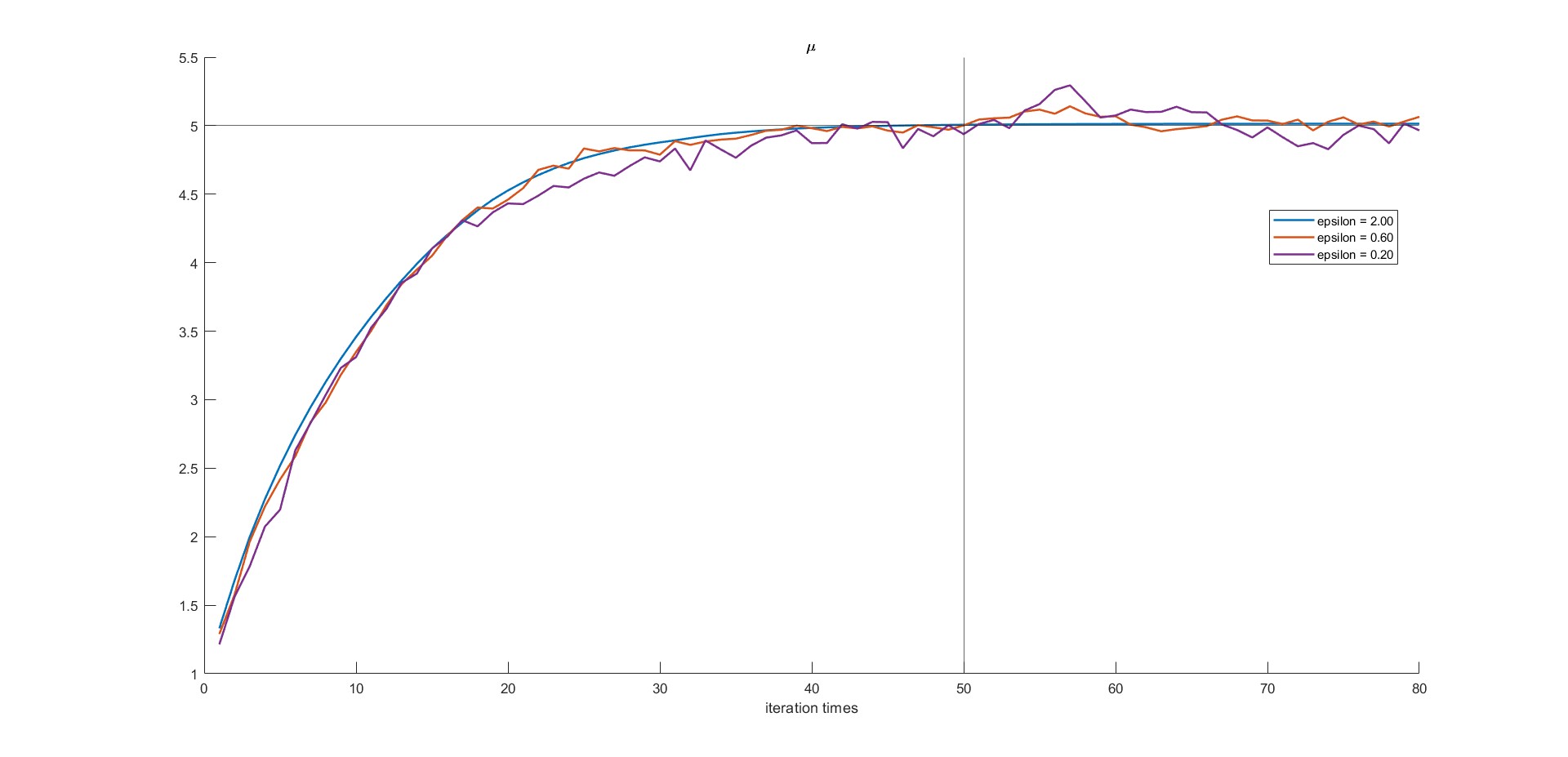
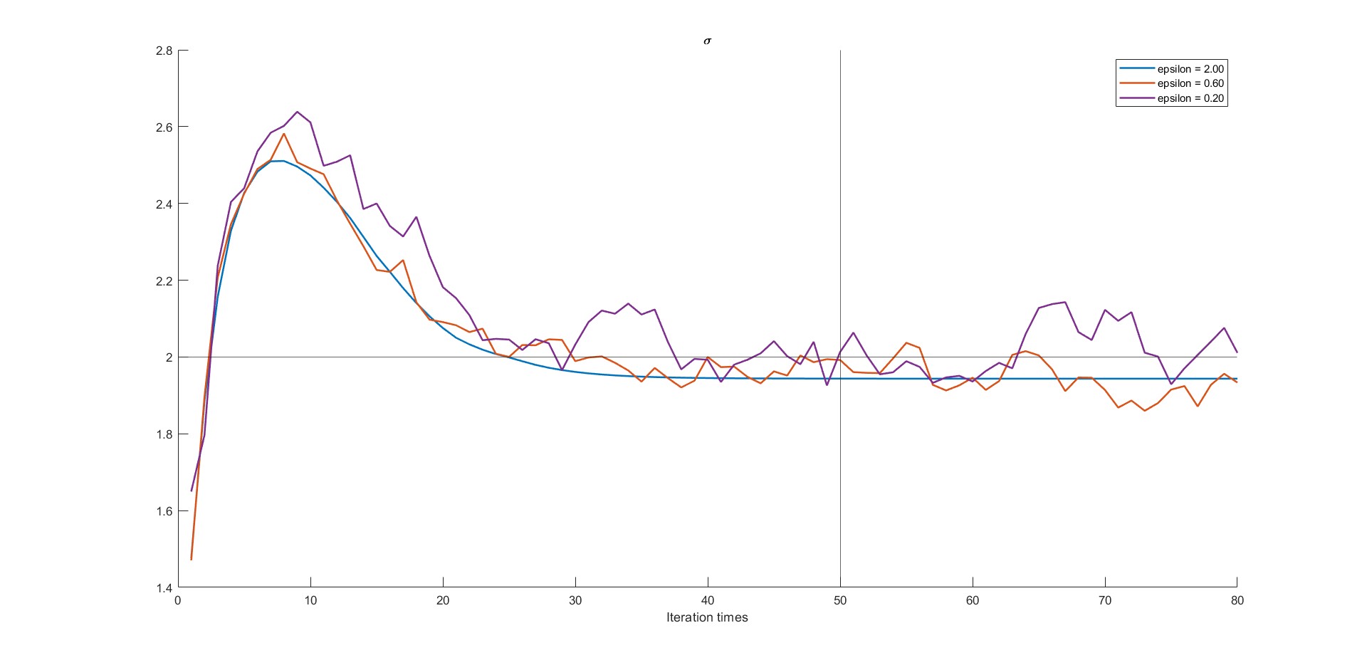
Figure 1: Private gradient descent path

Figure 2: Private gradient descent trajectory

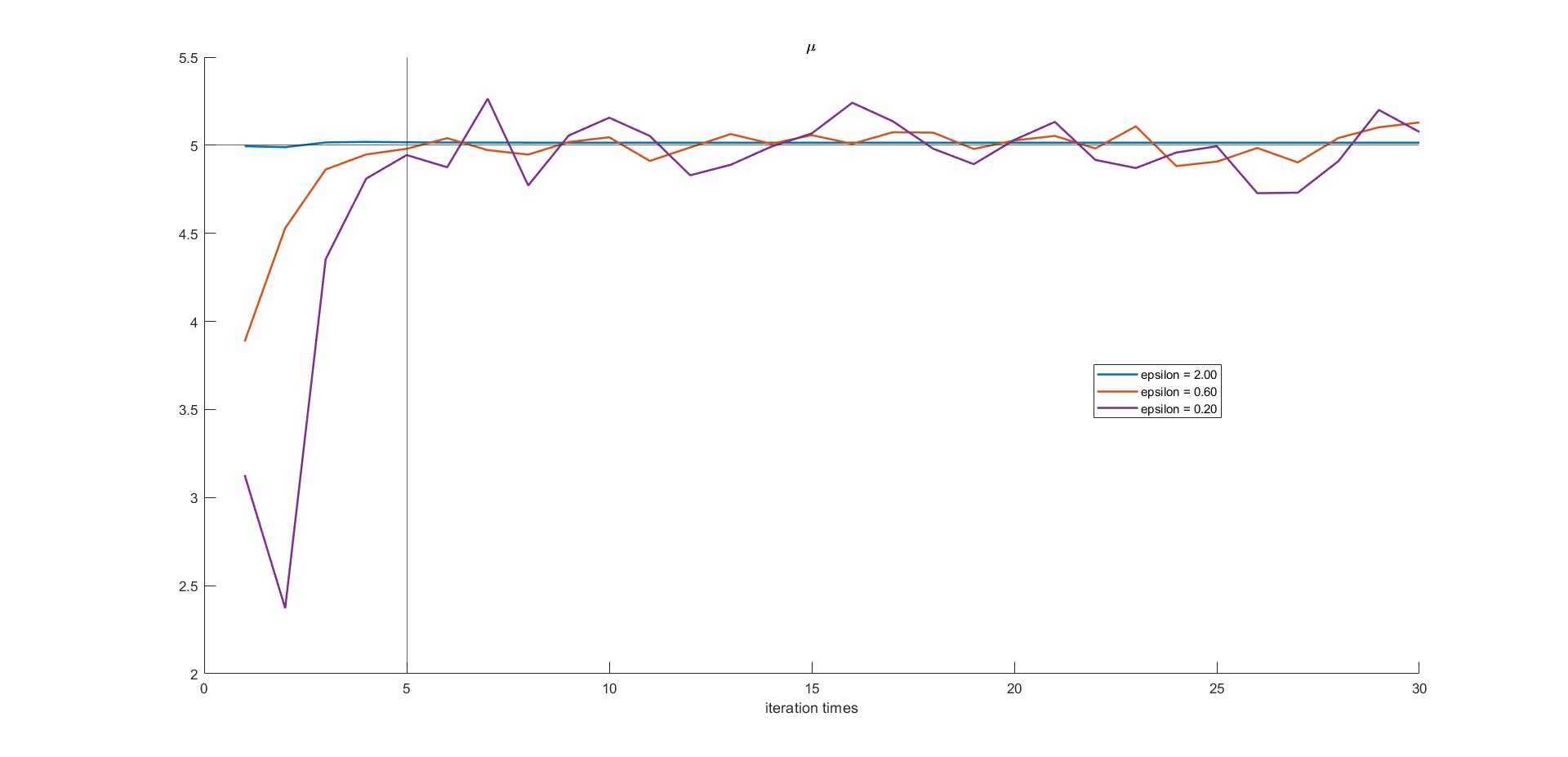
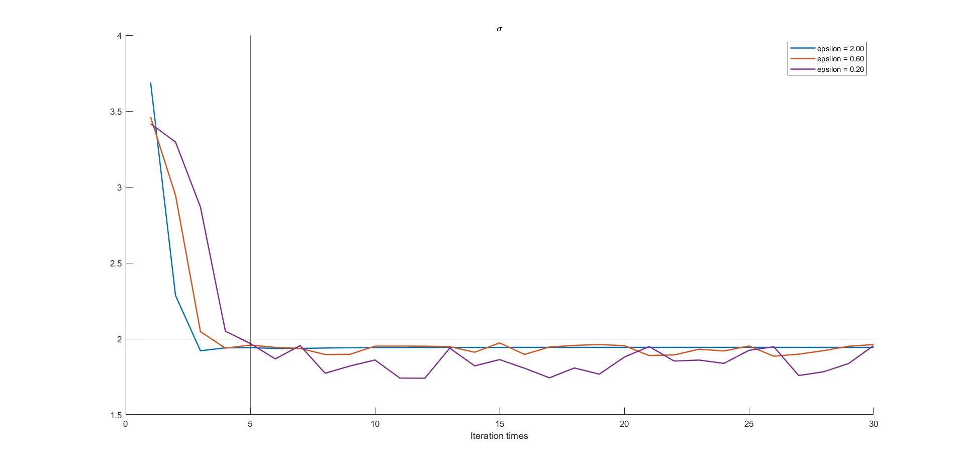
Figure 3: Private Newton’s method path

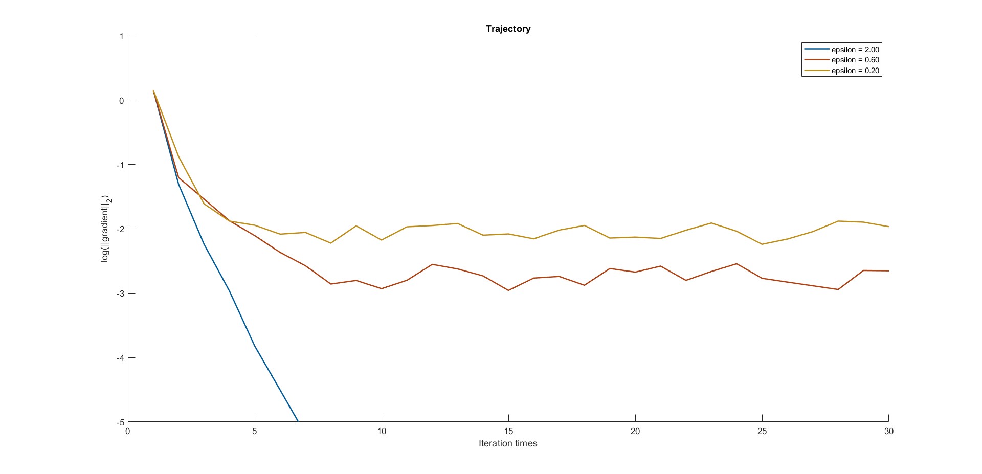
Figure 4: Private Newton’s method trajectory

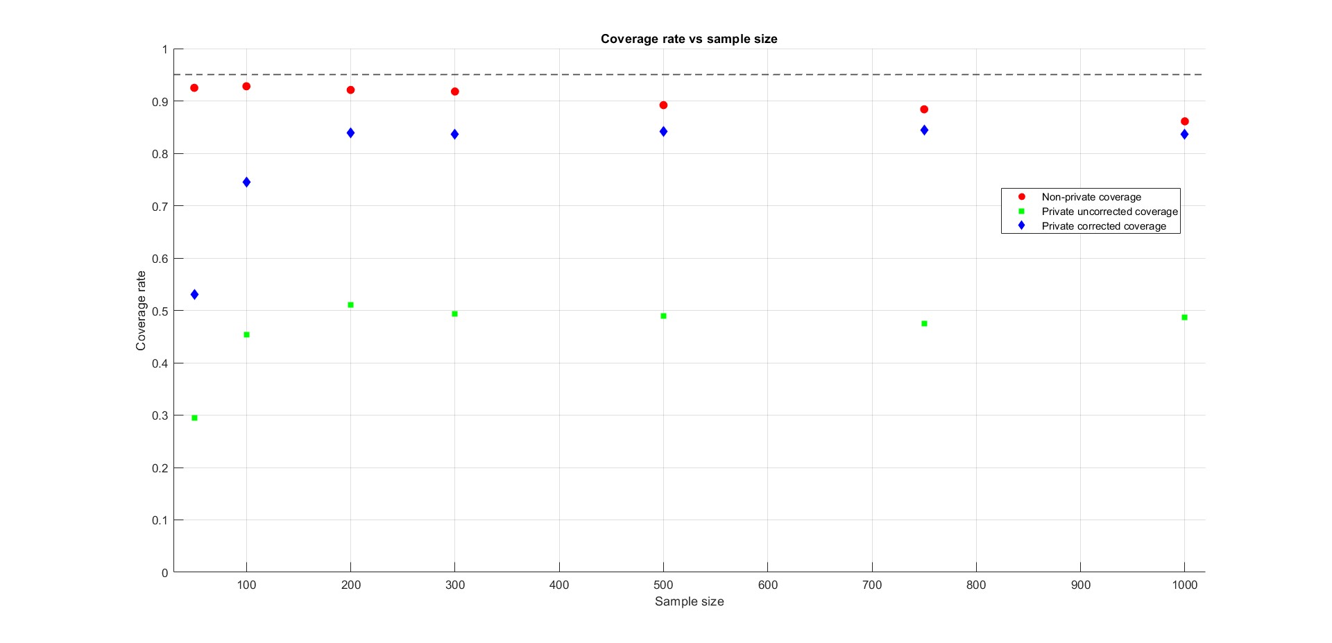
Figure 5: Private and non-private gradient descent 95% confidence interval coverage

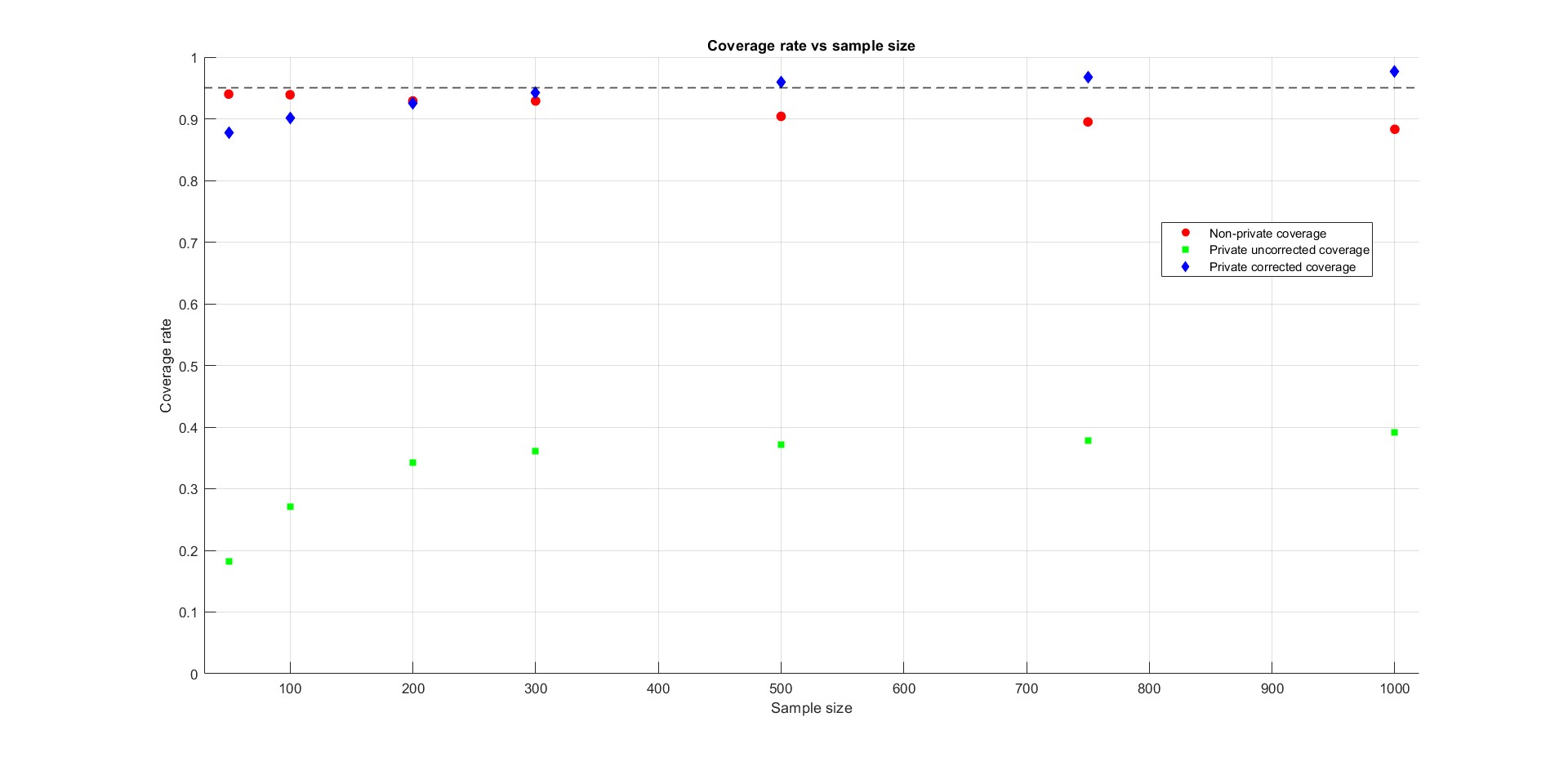
Figure 6: Private and non-private Newton’s method 95% confidence interval coverage

Robustness: We now describe the robustness properties of PMHDE by investigating the behavior under a gross-error contamination model. Denote by $f_{\bm{\theta},\alpha}$ the contamination model,

$$f_{\bm{\theta},\alpha}(x)=(1-\alpha)f_{\bm{\theta}}(x)+\alpha U_{z},$$

where $\alpha U_{z}$ is the uniform density on the interval $[z-\kappa,z+\kappa]$ for a small $\kappa>0$. Note that $f_{\bm{\theta},\alpha}(x)$ represents $\alpha\%$ contamination with distant outliers. In our experiments, $U_{z}$ is the uniform density on $[q(0.985,f_{\bm{\theta}}),q(0.995,f_{\bm{\theta}})]$, where $q(0.985,f_{\bm{\theta}})$ is the 98.5% quantile of $f_{\bm{\theta}}$ and $q(0.995,f_{\bm{\theta}})$ is the 99.5% quantile of $f_{\bm{\theta}}$; that is, $[9.34,10.15]$. We apply varying contamination levels with $\alpha=0,0.05,0.1,0.2,0.3$ for both PGD and PNR Algorithms. The result for the PGD algorithm is shown in Table 5, while that for the PNR algorithm is shown in Table 6.

We note that at high privacy levels, the iterative algorithm will yield estimates with high variability or tend to deviate from the true value since noise with larger variance is introduced in each iteration. This phenomenon is more common when the sample sizes are smaller. In these cases, it is common to use a thresholding strategy, which results in data in the extreme tails being suppressed. One approach to establishing the thresholds is by looking at the extreme tails of non-private estimators, while other methods are also feasible. In Appendix E, we provide numerical experiments illustrating the behavior of private estimators for different sample sizes (ranging from 200 to 500) and privacy levels.

Turning to Table 6 last row ($\epsilon=0.2$), we note that the standard error for PMHDE is larger due to aberrant values of the private estimate of $\mu$ in certain data sets. It turns out, in the no contamination case, 35 out of 5000 experiments yield estimates of private $\mu$ that are much larger than 10 or smaller than 0.15, while the true value is 5. In these cases, the usefulness of the estimate is in question. In applied settings, it is common not to release such values, and ad-hoc measures are adopted to circumvent this problem. We used the lower 0.7% and upper 99.5% percentiles of a Gaussian distribution with non-private $\hat{\mu}_{n}$ and $\hat{\sigma}_{n}$ to threshold the private estimates. This resulted in the following estimates for the case $\epsilon=0.2$: 4.863(0.807), 5.012(0.838), 5.135(0.811), 5.3340(0.850), 5.4430(0.921). The results illustrate that PMHDE retains robustness (compared to MLE) even under contamination.

	Contamination percentage $\alpha$
	0%	5%	10%	20%	30%
MLE (Std. Error)	5.001 (0.063)	5.241 (0.061)	5.476 (0.059)	5.952 (0.056)	6.422 (0.052)
PMHDE $\epsilon=2$ (Std. Error)	4.991 (0.083)	5.159 (0.089)	5.291 (0.09)	5.52 (0.095)	5.715 (0.102)
PMHDE $\epsilon=0.6$ (Std. Error)	4.986 (0.199)	5.158 (0.203)	5.289 (0.204)	5.516 (0.207)	5.712 (0.214)
PMHDE $\epsilon=0.2$ (Std. Error)	4.992 (0.353)	5.15 (0.349)	5.288 (0.355)	5.494 (0.367)	5.675 (0.523)

Table 5: Contamination results, gradient descent, sample size is 1000, $\mu=5$.

	Contamination percentage $\alpha$
	0%	5%	10%	20%	30%
MLE (Std. Error)	5.001 (0.063)	5.241 (0.061)	5.476 (0.059)	5.952 (0.056)	6.422 (0.052)
PMHDE $\epsilon=2$ (Std. Error)	5 (0.08)	5.174 (0.085)	5.309 (0.087)	5.555 (0.091)	5.778 (0.096)
PMHDE $\epsilon=0.6$ (Std. Error)	4.952 (0.326)	5.119 (0.333)	5.252 (0.341)	5.472 (0.38)	5.646 (0.42)
PMHDE $\epsilon=0.2$ (Std. Error)	4.942 (13.391)	4.905 (5.895)	5.054 (2.78)	5.349 (4.023)	5.169 (15.035)

Table 6: Contamination results, Newton-Raphson, sample size is 1000, $\mu=5$

5 Extensions and concluding remarks

In this paper, we developed new differential privacy concepts called $\epsilon-$HDP and $(\lambda,\epsilon)-$PDP and illustrated the optimality of $\epsilon-$HDP within the class of all power divergence measures for comparing two densities. We used these concepts to develop PMHDE estimators, which are not only robust and efficient but also private. These estimators are derived by privatizing the classical gradient descent and Newton-Raphson algorithms via a Gaussian mechanism. We analyzed the convergence properties of these algorithms and established that the resulting estimators are private, efficient, and robust. Since the models do not satisfy the strong convexity properties, we utilize ASLSC and smoothness derived from standard assumptions to analyze the resulting estimators.

Our methods also work when the Gaussian mechanism is replaced by the Laplace mechanism. Almost all properties in Theorem 3.2, Theorem 3.3, and Theorem 3.4 go through if one uses concentration bounds for Laplace random variables. Our initial analysis suggests that, in Theorem 3.2 and Theorem 3.3, the utility takes the following form: $||\hat{\bm{\theta}}_{n}^{(K_{n})}-\hat{\bm{\theta}}_{n}||_{2}=O_{p}\left(n^{-\frac{1}{p}}K_{n}^{\frac{1}{2}}\log(K_{n})\right)$ which also yields efficiency without any change. A detailed analysis of this case with a concentration inequality for the Laplace random variables and other probabilistic properties of compositions, especially when the number of queries diverges, will be discussed elsewhere.

It is also possible to extend the results to other minimum divergence estimators, such as minimum negative exponential disparity estimators, blended weight Hellinger distance estimators, and recently developed $S-$estimators (see Ghosh and Basu (2017)). We have not carried out all the technical details carefully; however, an initial heuristic analysis shows analogous versions of our results will continue to hold for each case. A unified approach for all these estimators under minimal conditions would be useful and is being studied by the authors.

Finally, replacing the power divergence with a general convex function to define an extended notion of privacy is also useful. However, obtaining closed-form expressions for the variance in the additive mechanism presents certain technical challenges.

6 Proof

In this section we provide the proofs of the main results of the paper.

6.1 Proof of Theorem 2.1 and 2.3

We start with the proof of Theorem 2.1. We begin with the case $\lambda(\lambda+1)\neq 0$. Since $M_{1}(w,D)$ is $(\lambda,\epsilon)$-PDP, the power divergence between $M_{1}(w,D)$ and $M_{1}(w,D^{\prime})$ is atmost $\epsilon_{1}$. For brevity, we denote the random variables $M_{1}(w,D)$ and $M_{1}(w,D^{\prime})$ by $X_{1}$ and $X_{2}$ respectively. Let $p_{1}(\cdot)$ and $p_{2}(\cdot)$ denote their densities. Thus, by the $(\lambda,\epsilon)-$ PDP property it follows that,

$$\frac{1}{\lambda(\lambda+1)}\mathbf{E}_{p_{2}}\left[\left(\frac{p_{1}(X_{2})}{p_{2}(X_{2})}\right)^{\lambda}\right]\leq\epsilon_{1}+\frac{1}{\lambda(\lambda+1)}$$ (6.1)

Next, let the random variables $Y_{1}|X_{1}$ and $Y_{2}|X_{2}$ represent the compositions of mechanisms $M_{2}(M_{1}(w,D),D)$ given $M_{1}(w,D)$ and $M_{2}(M_{1}(w,D^{\prime}),D^{\prime})$ given $M_{1}(w,D^{\prime})$ with conditional densities $q_{Y_{1}|X_{1}}(\cdot)$ and $q_{Y_{2}|X_{2}}(\cdot)$ respectively. Again using the PDP property, it follows that for a generic random variable $V\sim q_{Y_{2}|X_{2}}(\cdot)$,

$$\frac{1}{\lambda(\lambda+1)}\mathbf{E}_{q_{Y_{2}|X_{2}}}\left[\left(\frac{q_{Y_{1}|X_{1}}(V)}{q_{Y_{2}|X_{2}}(V)}\right)^{\lambda}\right]\leq\epsilon_{2}+\frac{1}{\lambda(\lambda+1)}$$ (6.2)

Now, to calculate power divergence of $M^{(2)}(w,D)$ and $M^{(2)}(w,D^{\prime})$, we need to calculate the joint power divergence of $(X_{1},Y_{1})$ and $(X_{2},Y_{2})$. Now, using that the joint density is the product of conditional density and the marginal density, it follows that

$$D_{\lambda}(M^{(2)}(w,D),M^{(2)}(w,D^{\prime}))=\frac{1}{\lambda(\lambda+1)}\mathbf{E}_{p_{2}}\left\{\left(\frac{p_{1}(X_{2})}{p_{2}(X_{2})}\right)^{\lambda}\mathbf{E}_{q_{Y_{2}|X_{2}}}\left[\left(\frac{q_{Y_{1}|X_{1}}(V)}{q_{Y_{2}|X_{2}}(V)}\right)^{\lambda}\right]\right\}-\frac{1}{\lambda(\lambda+1)}.$$

Now, suppose $\lambda(\lambda+1)>0$. Then, using (6.1) and (6.2) it follows that

$$D_{\lambda}(M^{(2)}(w,D),M^{(2)}(w,D^{\prime})) \leq \frac{1}{\lambda(\lambda+1)}[\epsilon_{1}(\lambda(\lambda+1))+1][\epsilon_{2}(\lambda(\lambda+1))+1]-\frac{1}{\lambda(\lambda+1)},$$

$$= \epsilon_{1}+\epsilon_{2}+\lambda(\lambda+1)\epsilon_{1}\epsilon_{2}.$$

Next, if $\lambda(\lambda+1)<0$, then using the condition $0<\epsilon<-[\lambda(\lambda+1)]^{-1}$ the above inequality continues to hold. Finally, consider the case $\lambda=0$. In this case, the power divergence reduces to the Kullback Leibler (KL) divergence between the densities. Hence, using the PDP property, it follows that

$$D_{0}(p_{1},p_{2})=KL(p_{1},p_{2})\leq\epsilon_{1},~~\text{and}~~D_{0}(q_{Y_{1}|X_{1}},q_{Y_{2}|X_{2}})=KL(q_{Y_{1}|X_{1}},q_{Y_{2}|X_{2}})\leq\epsilon_{2}.$$

Hence, with $V\sim q_{Y_{1}|X_{1}}(\cdot)$, we have

$$D_{\lambda}(M^{(2)}(w,D),M^{(2)}(w,D^{\prime}))=\mathbf{E}_{p_{1}}\left[\log\frac{p_{1}(X_{2})}{p_{2}(X_{2})}\right]+\mathbf{E}_{q_{Y_{1}|X_{1}}}\left[\log\frac{q_{Y_{1}|X_{1}}(V)}{q_{Y_{2}|X_{2}}(V)}\right]\leq\epsilon_{1}+\epsilon_{2}.$$

The proof of the case $\lambda=-1$ is similar. This completes the proof of (1). Next, the proof of (2) follows exactly as in (1) except that $M_{2}(X_{1},D)|X_{1}$ and $M_{2}(X_{2},D^{\prime})|X_{2}$ are now replaced by $M_{2}(w,D)$ and $M_{2}(w,D^{\prime})$. That is, we replace $\frac{q_{Y_{1}|X_{1}}(V)}{q_{Y_{2}|X_{2}}(V)}$ in (6.2) by $\frac{q_{Y_{1}}(V)}{q_{Y_{2}}(V)}$, where $q_{Y_{1}}$ and $q_{Y_{2}}$ are the unconditional distributions of $M_{2}(w,D)$ and $M_{2}(w,D^{\prime})$ respectively and $V$ has the density $q_{Y_{2}}$.

To start the proof of part (3), we first notice that adjacent $\mathbf{D}^{(2)}$ and $\mathbf{D}^{(2)^{\prime}}$ can be decomposed into two distinct cases. By definition,

$$||\mathbf{D}^{(2)}-\mathbf{D}^{(2)^{\prime}}||_{H}=\sum_{i=1}^{2}||D_{i}-D_{i}^{\prime}||_{H}=1.$$

Since the Hamming distance is a non-negative integer, the above equation holds if either: Case (1): $||D_{1}-D_{1}^{\prime}||_{H}=1$ and $||D_{2}-D_{2}^{\prime}||_{H}=0$; or Case (2): $||D_{1}-D_{1}^{\prime}||_{H}=0$ and $||D_{2}-D_{2}^{\prime}||_{H}=1$. Let, as before, $p_{1}(\cdot)$, $p_{2}(\cdot)$ denote the distributions of $M_{1}(w_{1},D_{1})$, $M_{1}(w_{1},D_{1}^{\prime})$. Also, let $q_{1}(\cdot)$, and $q_{2}(\cdot)$ are density functions of $M_{2}(w_{2},D_{2})$ and $M_{2}(w_{2},D_{2}^{\prime})$ respectively. The joint density of $M^{(2)}(\mathbf{W}^{(2)},\mathbf{D}^{(2)})$ and $M^{(2)}(\mathbf{W}^{(2)},\mathbf{D}^{(2)^{\prime}})$ are therefore given by $h_{1}(x,y)$ and $h_{2}(x,y)$ respectively, where $h_{1}(x,y)=p_{1}(x)q_{1}(y)$ and $h_{2}(x,y)=p_{2}(x)q_{2}(y)$.

If case (1) happens, $q_{1}(\cdot)=q_{2}(\cdot)$ holds since $D_{2}=D_{2}^{\prime}$. This leads to $\frac{h_{1}(x,y)}{h_{2}(x,y)}=\frac{p_{1}(x)}{p_{2}(x)}$. The PD between $M^{(2)}(\mathbf{W}^{(2)},\mathbf{D}^{(2)})$ and $M^{(2)}(\mathbf{W}^{(2)},\mathbf{D}^{(2)^{\prime}})$ is reduced to the PD between $M_{1}(w_{1},D_{1})$ and $M_{1}(w_{1},D_{1}^{\prime})$, since

$$D_{\lambda}(M^{(2)}(\mathbf{W}^{(2)},\mathbf{D}^{(2)}),M^{(2)}(\mathbf{W}^{(2)},\mathbf{D}^{(2)^{\prime}}))= \frac{1}{\lambda(\lambda+1)}\mathbf{E}_{h_{2}}\left[\left(\frac{h_{1}(X,Y)}{h_{2}(X,Y)}\right)^{\lambda}-1\right]$$

$$= \frac{1}{\lambda(\lambda+1)}\mathbf{E}_{p_{2}}\left[\left(\frac{p_{1}(X)}{p_{2}(X)}\right)^{\lambda}-1\right]$$

$$= D_{\lambda}(M_{1}(w_{1},D_{1}),M_{1}(w_{1},D_{1}^{\prime}))\leq\epsilon_{1}.$$

The last inequality follows from $M_{1}(w_{1},D_{1})$ is $(\lambda,\epsilon_{1})-$PDP. Similarly in Case (2),

$$D_{\lambda}(M^{(2)}(\mathbf{W}^{(2)},\mathbf{D}^{(2)}),M^{(2)}(\mathbf{W}^{(2)},\mathbf{D}^{(2)^{\prime}}))=D_{\lambda}(M_{2}(w_{2},D_{2}),M_{2}(w_{2},D_{2}^{\prime}))\leq\epsilon_{2}.$$

Combining Case (1) and Case (2) together, we get $D_{\lambda}(M^{(2)}(\mathbf{W}^{(2)},\mathbf{D}^{(2)}),M^{(2)}(\mathbf{W}^{(2)},\mathbf{D}^{(2)^{\prime}}))\leq\max\{\epsilon_{1},\epsilon_{2}\}$, which implies that the parallel composition $M^{(2)}(\mathbf{W}^{(2)},\mathbf{D}^{(2)})$ is $(\lambda,\max\{\epsilon_{1},\epsilon_{2}\})-$PDP. This completes the proof of Theorem 2.1. The Proof of Theorem 2.3 follows by taking $\lambda=-\frac{1}{2}$ and noticing that the objective function is $D_{-\frac{1}{2}}(\cdot,\cdot)=2D_{HD}^{2}(\cdot,\cdot)$.    

6.2 Proof of Theorem 2.2 and Proposition 2.2

We begin with the case when $Y_{i}$’s are $N(0,\sigma^{2})$. In this case, using Lemma B.1 we have that

$$D_{\lambda}(M(w,D),M(w,D^{\prime})) = \frac{1}{\lambda(\lambda+1)}\left[e^{\frac{\lambda(\lambda+1)||\mathbf{v}||_{2}^{2}}{2\sigma^{2}}}-1\right],$$

where $\mathbf{v}$ is the difference between the mean of $M(w,D)$ and the mean of $M(w,D^{\prime})$, and for $r=1,2$, $||\mathbf{v}||_{r}=\Delta_{L_{r}}W$. Thus, $D_{\lambda}(M(w,D),M(w,D^{\prime}))\leq\epsilon$ is equivalent to

$$\sigma\geq||\mathbf{v}||_{2}\sqrt{\frac{\lambda(\lambda+1)}{2\log(1+\lambda(\lambda+1)\epsilon)}},$$

which is well-defined for all values of $0<\epsilon<[-\lambda(\lambda+1)]^{-1}$. Thus, we choose

$$\sigma^{2}_{\lambda,\epsilon}=(\Delta_{L_{2}}W)^{2}\frac{\lambda(\lambda+1)}{2\log(1+\lambda(\lambda+1)\epsilon)}.$$

Next, when $\lambda=0$,

$$D_{0}(M(w,D),M(w,D^{\prime}))=\sum_{i=1}^{m}\frac{||w_{1}-w_{2}||_{2}^{2}}{2\sigma^{2}}$$

Again, $D_{0}{M(w,D),M(w,D^{\prime})}\leq\epsilon$ is equivalent to

$$\sigma^{2}_{0,\epsilon}=\frac{(\Delta_{L_{2}}W)^{2}}{2\epsilon}.$$

The case for $\lambda=-1$ is similar. Next, turning to the Laplace case, using Lemma B.2, notice that

$$D_{\lambda}(M(w,D),M(w,D^{\prime})) = \frac{1}{\lambda(\lambda+1)}\left[\left(\prod_{i=1}^{m}\int_{\mathbb{R}}\frac{1}{2b}e^{-\frac{(\lambda+1)|y_{i}-v_{i}|-\lambda|y_{i}|}{b}}\mathrm{d}y_{i}\right)-1\right]$$

$$\leq \frac{1}{\lambda(\lambda+1)}\left[e^{\frac{sign(\lambda)(\lambda+1)||v||_{1}}{b}}-1\right].$$

Similarly,

$$D_{\lambda}(M(w,D^{\prime}),M(w,D))\leq\frac{1}{\lambda(\lambda+1)}\left[e^{\frac{sign(\lambda+1)(\lambda)||v||_{1}}{b}}-1\right].$$

Thus, $D_{\lambda}(M(w,D),M(w,D^{\prime}))\leq\epsilon$ is equivalent to

$$b\geq\max\left\{\frac{sign(\lambda)(\lambda+1)||v||_{1}}{\log(\lambda(\lambda+1)\epsilon+1)},\frac{sign(\lambda+1)(\lambda)||v||_{1}}{\log(\lambda(\lambda+1)\epsilon+1)}\right\}.$$

Thus, we choose $b_{\lambda,\epsilon}$ to be

$$b_{\lambda,\epsilon}=\max\left\{\frac{sign(\lambda)(\lambda+1)\Delta_{L_{1}}W}{\log(\lambda(\lambda+1)\epsilon+1)},\frac{sign(\lambda+1)(\lambda)\Delta_{L_{1}}W}{\log(\lambda(\lambda+1)\epsilon+1)}\right\}.$$

Turning to the case $\lambda(\lambda+1)=0$, we note that

$$D_{0}(M(w,D),M(w,D^{\prime})) = \sum_{i=1}^{m}\int_{\mathbb{R}}\frac{1}{2b}e^{-\frac{|y_{i}|}{b}}\cdot\frac{|y_{i}-v_{i}|-|y_{i}|}{b}\mathrm{d}y_{i}$$

$$\leq \frac{||w_{1}-w_{2}||_{1}}{b}$$

Hence, $D_{0}(M(w,D),M(w,D^{\prime}))\leq\epsilon$ implies $b\geq\frac{\Delta w}{\epsilon}$. Thus,

$$b_{0,\epsilon}=\frac{\Delta_{L_{1}}W}{\epsilon}.$$

The proof for the case $\lambda=-1$ is similar. Finally, the proof for the HDP case follows by taking $\lambda=-\frac{1}{2}$ and replacing $\epsilon$ by $2\epsilon$ to obtain $\epsilon-$HDP.    

6.3 Proof of Corollary 2.1

The proof is based on the following iterative argument for adaptive and sequential compositions. Setting $\epsilon_{1}=\epsilon$ and $\epsilon_{2}=h_{1}(\epsilon)$ it follows from Theorem 2.3 part 1. and part 2., that $h_{2}(\epsilon)=\epsilon+h_{1}(\epsilon)-\frac{1}{2}\epsilon h_{1}(\epsilon)$. Now iterating, we obtain $h_{j+1}(\epsilon)=\epsilon+h_{j}(\epsilon)-\frac{1}{2}\epsilon h_{j}(\epsilon)$. The proof for the parallel compositions follows from part 3. of Theorem 2.3.    

6.4 Proof of Proposition 2.1

The proof of the Proposition follows using a comparison argument. Recall that the total variation distance between two densities can be expressed as one-half the $L_{1}-$norm, which is bounded above by the Hellinger distance between the densities. That is,

$$TV(p_{1},p_{2})=\frac{1}{2}||p_{1}-p_{2}||_{1}\leq HD(p_{1},p_{2}).$$

Now, if $HD^{2}(p_{1},p_{2})\leq\epsilon$, then $TV(p_{1},p_{2})\leq\sqrt{\epsilon}$ which implies that $M(\cdot,\cdot)$ satisfies $\sqrt{\epsilon}-$TV privacy. Hence, using Ghazi and Issa (2024) page 209, it follows that $M$ also satisfies $(0,\sqrt{\epsilon})$ differential privacy. Turning to $\mu-$GDP, we now use the Corollary 1 in Dong et al. (2022) to get $\mu=2\Phi^{-1}(\frac{\sqrt{\epsilon}+1}{2})$.    

6.5 Proof of Theorem 2.4

First notice that by the definition of group privacy, we need to calculate $D_{HD}(M(w,D),M(w,D^{\prime}))$ for $k-$ neighbor datasets $D$ and $D^{\prime}$. Now, by definition of $k-$neighbor datasets, there exist $D=B_{0},B_{1},B_{2},\cdots B_{k}=D^{\prime}$, such that $||B_{i}-B_{i+1}||_{H}=1$ for all $i=0,1,\cdots,(k-1)$. Also, since $M(w,B_{i})$ is $\epsilon-$ HDP for all $0\leq i\leq k$, we get that

$$D_{HD}(M(w,B_{i}),M(w,B_{i+1}))\leq\epsilon.$$

Now, using that $D_{HD}^{\frac{1}{2}}(\cdot,\cdot)=HD(\cdot,\cdot)$ is a metric, using the triangle inequality

$${}D_{HD}^{\frac{1}{2}}(M(w,D),M(w,D^{\prime}))\leq\sum_{i=1}^{k}D_{HD}^{\frac{1}{2}}(M(w,B_{i-1}),M(w,B_{i}))\leq k\sqrt{\epsilon}.$$ (6.3)

The result follows by squaring both sides of (6.3).    

6.6 Proof of Proposition 3.6

To show $H_{n}(\bm{\theta})$ is $\alpha-$ Lipschitz continuous, it is enough to show that the $(i,j)^{th}$ component of $H_{n}(\bm{\theta})$ is Lipschitz continuous for all $(i,j)$, where the Lipschitz constant depends only on $m$ and the upper bounds in assumptions (U1) and (U2). That is, we will show that for any $\bm{\theta}^{(1)},\bm{\theta}^{(2)}\in\Theta$,

$$|H_{n,i,j}(\bm{\theta}^{(1)})-H_{n,i,j}(\bm{\theta}^{(2)})|\leq\alpha_{i,j}||\bm{\theta}^{(1)}-\bm{\theta}^{(2)}||_{2},$$

where $H_{n,i,j}(\bm{\theta})$ is the $(i,j)^{th}$ component of $H_{n}(\bm{\theta})$. Recall that

$$H_{n,i,j}(\bm{\theta})= -\int_{\mathbb{R}}g_{n}^{\frac{1}{2}}(x)f_{\bm{\theta}}^{\frac{1}{2}}(x)u_{\bm{\theta},j}(x)u_{\theta,i}(x)\mathrm{d}x-2\int_{\mathbb{R}}g_{n}^{\frac{1}{2}}(x)f_{\bm{\theta}}^{\frac{1}{2}}(x)u_{\bm{\theta},i,j}(x)\mathrm{d}x.$$

Then for any $\bm{\theta}^{(1)},\bm{\theta}^{(2)}\in\Theta$,

$$|H_{n,i,j}(\bm{\theta}^{(1)})-H_{n,i,j}(\bm{\theta}^{(2)})| \leq \int_{\mathbb{R}}g_{n}^{\frac{1}{2}}(x)|T_{1,i,j}(\bm{\theta}^{(1)},x)-T_{1,i,j}(\bm{\theta}^{(2)},x)|\mathrm{d}x$$ (6.4)

$$+2\int_{\mathbb{R}}g_{n}^{\frac{1}{2}}(x)|T_{2,i,j}(\bm{\theta}^{(1)},x)-T_{2,i,j}(\bm{\theta}^{(2)},x)|\mathrm{d}x,$$

where

$$T_{1,i,j}(\bm{\theta},x)=f_{\theta}^{\frac{1}{2}}(x)u_{\bm{\theta},j}(x)u_{\bm{\theta},i}(x),\quad T_{2,i,j}(\bm{\theta},x)=f_{\bm{\theta}}^{\frac{1}{2}}(x)u_{\bm{\theta},i,j}(x).$$

Notice that for $\bm{\theta}\in\Theta$, $T_{1,i,j}(\bm{\theta},x)$ and $T_{2,i,j}(\bm{\theta},x)$ are differentiable in $\bm{\theta}$ by Assumption (U2). Using Cauchy-Schwarz inequality and the upper bounds in Assumption (U2), for $\bm{\theta}\in\Theta$ we obtain that $g_{n}^{1/2}(x)||\nabla T_{1,i,j}(\bm{\theta},x)||_{2}$ and $g_{n}^{1/2}(x)||\nabla T_{2,i,j}(\bm{\theta},x)||_{2}$ are integrable with respect to $x$, where the gradient is taken with respect to $\bm{\theta}$. By the mean value theorem and Cauchy-Schwarz inequality, there exists $\bm{\theta}^{(1)*}$ and $\bm{\theta}^{(2)*}$ on the line between $\bm{\theta}^{(1)}$ and $\bm{\theta}^{(2)}$, such that

$$|T_{1,i,j}(\bm{\theta}^{(1)},x)-T_{1,i,j}(\bm{\theta}^{(2)},x)|\leq ||\nabla T_{1,i,j}(\bm{\theta}^{(1)*},x)||_{2}\cdot||\bm{\theta}^{(1)}-\bm{\theta}^{(2)}||_{2}$$ (6.5)

$$|T_{2,i,j}(\bm{\theta}^{(1)},x)-T_{2,i,j}(\bm{\theta}^{(2)},x)|\leq ||\nabla T_{2,i,j}(\bm{\theta}^{(2)*},x)||_{2}\cdot||\bm{\theta}^{(1)}-\bm{\theta}^{(2)}||_{2}.$$ (6.6)

By the convexity of $\Theta$ (see Assumption (A1)), we obtain $\bm{\theta}^{(1)*},\bm{\theta}^{(2)*}\in\Theta$. Now, multiplying both sides of (6.5) and (6.6) by $g_{n}^{\frac{1}{2}}(\cdot)$ and using the integrability described above, it follows that

$$\int g_{n}^{1/2}(x)||\nabla T_{1,i,j}(\bm{\theta},x)||_{2}\mathrm{d}x\leq\left(\sup_{\bm{\theta}\in\Theta}\int g_{n}^{1/2}(x)||\nabla T_{1,i,j}(\bm{\theta},x)||_{2}\mathrm{d}x\right)||\bm{\theta}_{1}-\bm{\theta}_{2}||_{2}.$$

Using similar arguments for $T_{2,i,j}$ and setting

$$0<\alpha_{i,j}=\sup_{\bm{\theta}\in\Theta}\left\{\int g_{n}^{1/2}(x)||\nabla T_{1,i,j}(\bm{\theta},x)||_{2}\mathrm{d}x+2\int g_{n}^{1/2}(x)||\nabla T_{2,i,j}(\bm{\theta},x)||_{2}\mathrm{d}x\right\}<\infty.$$

It follows that

$$|H_{n,i,j}(\bm{\theta}^{(1)})-H_{n,i,j}(\bm{\theta}^{(2)})|\leq\alpha_{i,j}||\bm{\theta}^{(1)}-\bm{\theta}^{(2)}||_{2}.$$

This completes the proof.    

Before we prove the theorem, we recall that

$$g_{n}(x)=\frac{1}{nc_{n}}\sum_{i=1}^{n}K\left(\frac{x-X_{i}}{c_{n}}\right).$$

and for the neighboring i.i.d. observations $\{X^{\prime}_{1},X_{2},\cdots,X_{n}\}$, the corresponding density estimator is

$$\tilde{g}_{n}(x)=\frac{1}{nc_{n}}\sum_{i=2}^{n}K\left(\frac{x-X_{i}}{c_{n}}\right)+\frac{1}{nc_{n}}K\left(\frac{x-X^{\prime}_{1}}{c_{n}}\right).$$

The corresponding loss functions are given by

$$L_{n}(\bm{\theta})=2HD^{2}(g_{n},f_{\bm{\theta}})~~\text{and}~~\tilde{L}_{n}(\bm{\theta})=2HD^{2}(\tilde{g}_{n},f_{\bm{\theta}}),$$

and the Hessian of the loss functions are given by $H_{n}(\bm{\theta})$ and $\tilde{H}_{n}(\bm{\theta})$.

6.7 Proof of Proposition 3.7 and Theorem 3.1

We begin with the proof of (3.3). First, notice that for all $1\leq i\leq m$

$$\frac{\partial}{\partial\theta_{i}}L_{n}(\bm{\theta})=-2\int_{\mathbb{R}}g_{n}^{\frac{1}{2}}(x)f_{\bm{\theta}}^{\frac{1}{2}}(x)u_{\bm{\theta},i}(x)\mathrm{d}x$$

Hence,

$$\bar{\Delta}^{(i)}\coloneqq\frac{\partial}{\partial\theta_{i}}(L_{n}(\bm{\theta})-\tilde{L}_{n}(\bm{\theta}))= 2\int_{\mathbb{R}}(g_{n}^{\frac{1}{2}}(x)-\tilde{g}_{n}^{\frac{1}{2}}(x))f_{\bm{\theta}}^{\frac{1}{2}}(x)u_{\bm{\theta},i}(x)\mathrm{d}x$$

where we have suppressed $n$ in the notation $\bar{\Delta}^{(i)}$. Using Cauchy-Schwarz inequality, the $HD^{2}(g_{n},\tilde{g}_{n})$ is bounded above by $||g_{n}-\tilde{g}_{n}||_{1}$ and, assumption (A2) it follows that

$$\bar{\Delta}^{(i)}\leq 2HD(g_{n},\tilde{g}_{n})\cdot\left[\int_{\mathbb{R}}f_{\bm{\theta}}(x)u_{\bm{\theta},i}^{2}(x)\mathrm{d}x\right]^{1/2}\leq C_{i}||g_{n}-\tilde{g}_{n}||_{1}^{\frac{1}{2}}.$$

Now,

$$||g_{n}-\tilde{g}_{n}||_{1}^{1/2}=\left[\frac{1}{n\cdot c_{n}}\int_{\mathbb{R}}|K\left(\frac{x-X_{1}}{c_{n}}\right)-K\left(\frac{x-X_{1}^{\prime}}{c_{n}}\right)|\mathrm{d}x\right]^{1/2}\leq\left(\frac{2}{n}\right)^{1/2}.$$ (6.7)

Hence $\bar{\Delta}^{(i)}\leq 2C_{i}\left(\frac{2}{n}\right)^{1/2}$. Let $\mathbf{\bar{\Delta}}=[\bar{\Delta}^{(1)},\cdots,\bar{\Delta}^{(m)}]$. Then $\Delta_{L_{1}}(\nabla L_{n}(\bm{\theta}))\leq||\mathbf{\bar{\Delta}}||_{1}\leq C\cdot m\cdot n^{-\frac{1}{2}}$ and $\Delta_{L_{2}}(\nabla L_{n}(\bm{\theta}))\leq||\mathbf{\bar{\Delta}}||_{2}\leq C\cdot\sqrt{m}\cdot n^{-\frac{1}{2}}$, where $C=\max_{i}\{2\sqrt{2}C_{i}\}$.

We now turn to the Hessian. Recall the definition $u_{\bm{\theta},i}(x)=\frac{1}{f_{\bm{\theta}}(x)}\cdot\frac{\partial}{\partial\theta_{i}}f_{\bm{\theta}}(x)$, $u_{\bm{\theta},i,j}=\frac{\partial}{\partial\theta_{j}}u_{\bm{\theta},i}$, and

$$H_{n,i,j}(\bm{\theta})=-\int_{\mathbb{R}}g_{n}^{\frac{1}{2}}(x)f_{\bm{\theta}}^{\frac{1}{2}}(x)[u_{\bm{\theta},j}(x)u_{\bm{\theta},i}(x)+2u_{\bm{\theta},i,j}(x)]\mathrm{d}x.$$

Hence,

$$\bar{\Delta}^{(i,j)}\coloneqq H_{n,i,j}(\theta)-\tilde{H}_{n,i,j}(\theta)=\int_{\mathbb{R}}(g_{n}^{\frac{1}{2}}(x)-{\tilde{g}_{n}}^{\frac{1}{2}}(x))f_{\bm{\theta}}^{\frac{1}{2}}(x)[u_{\bm{\theta},j}(x)u_{\bm{\theta},i}(x)+2u_{\bm{\theta},i,j}(x)]\mathrm{d}x$$

Using Cauchy-Schwarz inequality, the $HD^{2}(g_{n},\tilde{g}_{n})$ is bounded above by $||g_{n}-\tilde{g}_{n}||_{1}$ and, assumptions (U1)-(U2) it follows that

$$|\bar{\Delta}^{(i,j)}|\leq 2HD(g_{n},\tilde{g}_{n})\cdot\left[\int_{\mathbb{R}}f_{\bm{\theta}}^{\frac{1}{2}}(x)[u_{\bm{\theta},j}(x)u_{\bm{\theta},i}(x)+2u_{\bm{\theta},i,j}(x)]\right]^{1/2}\leq(C_{i,1}+C_{i,2})||g_{n}-\tilde{g}_{n}||_{1}^{\frac{1}{2}},$$

where $C_{i,1}$ and $C_{i,2}$ are upper bounds given in assumptions (U1) and (U2). Using (6.7), it follows that $\bar{\Delta}^{(i,j)}\leq C_{i,j}\cdot n^{-\frac{1}{2}}$. Let $\mathbf{\bar{\Delta}}$ be a $m\times m$ matrix with $(i,j)^{\text{th}}$ element $\bar{\Delta}^{(i,j)}$. Then $\Delta_{L_{1}}(H_{n}(\bm{\theta}))\leq||\mathbf{\bar{\Delta}}||_{1}\leq C\cdot m\cdot n^{-\frac{1}{2}}$ and $\Delta_{L_{2}}(\nabla L_{n}(\bm{\theta}))\leq||\mathbf{\bar{\Delta}}||_{2}\leq C\cdot m\cdot n^{-\frac{1}{2}}$ for some $0<C<\infty$. This completes the proof of (3.3) and hence Proposition 3.7.

We next turn to the Proof of Theorem 3.1, specifically (3.8). In this case, we require the sensitivity is taken on a compact set $A_{n}$ as in assumption (U3). To reduce notational complexity, redefine $\tilde{g}_{n}(x)$ as follows:

$$\tilde{g}_{n}(x)=\frac{1}{nc_{n}}\sum_{i=2}^{n}K\left(\frac{x-X_{i}}{c_{n}}\right)\bm{1}_{(X_{i}\in B_{n})}+\frac{1}{nc_{n}}K\left(\frac{x-X^{\prime}_{1}}{c_{n}}\right)\bm{1}_{(X_{1}^{\prime}\in B_{n})},$$

where $X_{1},X_{1}^{\prime}\in B_{n}$. Now the $\bar{\Delta}^{(i)}$ is given by

$$\bar{\Delta}^{(i)}\coloneqq 2\int_{\mathbb{R}}(\bar{g}_{n}^{\frac{1}{2}}(x)-\tilde{g}_{n}^{\frac{1}{2}}(x))f_{\bm{\theta}}^{\frac{1}{2}}(x)u_{\bm{\theta},i}(x)\cdot{\bm{1}}_{(x\in A_{n})}\mathrm{d}x+2\int_{\mathbb{R}}(\bar{g}_{n}^{\frac{1}{2}}(x)-\tilde{g}_{n}^{\frac{1}{2}}(x))f_{\bm{\theta}}^{\frac{1}{2}}(x)u_{\bm{\theta},i}(x)\cdot{\bm{1}}_{(x\notin A_{n})}\mathrm{d}x$$

$$\coloneqq \bar{\Delta}^{(i,1)}+\bar{\Delta}^{(i,2)}.$$

Using the equation $a^{\frac{1}{2}}-b^{\frac{1}{2}}=\frac{a-b}{2b^{1/2}}-\frac{(a^{1/2}-b^{1/2})^{2}}{2b^{1/2}}$, and denoting $R_{\bm{\theta}}(x)=|f_{\bm{\theta}}^{1/2}(x)u_{\bm{\theta},i}(x)|$, we obtain

$$|\bar{\Delta}^{(i,1)}|\leq T_{1}+T_{2},\quad\text{where}$$

$$T_{1}=\int_{\mathbb{R}}\left|\frac{\bar{g}_{n}(x)-\tilde{g}_{n}(x)}{2\sqrt{\tilde{g}_{n}(x)}}\right|\cdot R_{\bm{\theta}}(x)\cdot{\bm{1}}_{(x\in A_{n})}\mathrm{d}x,~\text{and}~T_{2}=\int_{\mathbb{R}}\left|\frac{(\sqrt{\bar{g}_{n}(x)}-\sqrt{\tilde{g}_{n}(x)})^{2}}{2\sqrt{\tilde{g}_{n}(x)}}\right|\cdot R_{\bm{\theta}}(x)\cdot{\bm{1}}_{(x\in A_{n})}\mathrm{d}x.$$

We first develop the upper bound of $T_{1}$ and use the fact that $T_{2}\leq T_{1}$ almost surely to get the final answer. Using the Hölder’s inequality with $p\in(1,2)$ and integrability of $|R_{\bm{\theta}}(x)|^{q}$ in assumption (U3) and the boundedness of the kernel function $K(\cdot)$, it follows that

$$T_{1}\leq C_{1}\cdot\left[\int_{\mathbb{R}}\left|\frac{g_{n}(x)-\tilde{g}_{n}(x)}{2\sqrt{\tilde{g}_{n}(x)}}\right|^{p}\cdot{\bm{1}}_{(x\in A_{n})}\mathrm{d}x\right]^{\frac{1}{p}}$$

$$\leq C_{1}\cdot\left[\sup_{x\in A_{n}}\{|g_{n}(x)-\tilde{g}_{n}(x)|\}\right]^{\frac{1}{p}}\cdot\left[\int_{\mathbb{R}}\frac{|g_{n}(x)-\tilde{g}_{n}(x)|^{p-1}}{(2\sqrt{\tilde{g}_{n}(x)})^{p}}\cdot{\bm{1}}_{(x\in A_{n})}\mathrm{d}x\right]^{\frac{1}{p}}$$

$$\leq C_{1}\cdot C_{2}\left(\frac{1}{n}\right)^{\frac{1}{p}}\cdot\left[\int_{\mathbb{R}}\frac{|g_{n}(x)-\tilde{g}_{n}(x)|^{p-1}}{(2\sqrt{\tilde{g}_{n}(x)})^{p}}\cdot{\bm{1}}_{(x\in A_{n})}\mathrm{d}x\right]^{\frac{1}{p}}$$

where $0<C_{1}<\infty$ is a constant (independent of $\bm{\theta}$) obtained from assumption (U3). We turn to the last term on the RHS and show it converges to $0$ almost surely under assumption (U3). Notice that $\inf_{x\in A_{n}}\tilde{g}_{n}(x)\geq\delta_{n}$, we obtain

$$\int_{\mathbb{R}}\frac{|g_{n}(x)-\tilde{g}_{n}(x)|^{p-1}}{(2\sqrt{\tilde{g}_{n}(x)})^{p}}\cdot{\bm{1}}_{(x\in A_{n})}\mathrm{d}x\leq \int_{\mathbb{R}}\frac{|g_{n}(x)-\tilde{g}_{n}(x)|^{p-1}}{(2\sqrt{\delta_{n})^{p}}}\cdot{\bm{1}}_{(x\in A_{n})}\mathrm{d}x$$

$$\leq \frac{1}{(2\sqrt{\delta_{n}})^{p}\cdot(n\cdot c_{n})^{p-1}}\left[\int_{\mathbb{R}}\left|K(\frac{x-X_{1}^{\prime}}{c_{n}})-K(\frac{x-X_{1}}{c_{n}})\right|^{p-1}\mathrm{d}x\right]$$

Now we establish the upper bound of the last term on RHS. By assumption (A2), $K(\cdot)$ has compact support, say $[-\beta,\beta]$. In the calculation, fix any $X_{1}=x_{1}$, $X^{\prime}_{1}=x^{\prime}_{1}$ and $x_{1},x^{\prime}_{1}\in B_{n}$. Then write

$$S=supp_{x}\left(K(\frac{x-x_{1}}{c_{n}})\right)\cup supp_{x}\left(K(\frac{x-x_{1}^{\prime}}{c_{n}})\right)=[x_{1}-\beta c_{n},x_{1}+\beta c_{n}]\cup[x_{1}^{\prime}-\beta c_{n},x_{1}^{\prime}+\beta c_{n}]$$

and $\lambda(S)\leq 4\beta c_{n}$, where $\lambda(S)$ is the Lebesgue measure of $S$. Notice that $h(x)=x^{p-1}$ is concave for $p\in(1,2)$ on $x\in(0,\infty)$, using Jensen’s inequality, it follows that

$$\int_{\mathbb{R}}\left|K(\frac{x-x_{1}^{\prime}}{c_{n}})-K(\frac{x-x_{1}}{c_{n}})\right|^{p-1}\mathrm{d}x= \lambda(S)\int_{S}\left|K(\frac{x-x_{1}^{\prime}}{c_{n}})-K(\frac{x-x_{1}}{c_{n}})\right|^{p-1}\cdot\frac{1}{\lambda(S)}\mathrm{d}x$$

$$= \lambda(S)\mathbf{E}\left[\left|K(\frac{X-x_{1}^{\prime}}{c_{n}})-K(\frac{X-x_{1}}{c_{n}})\right|^{p-1}\right]$$

$$\leq \lambda(S)\mathbf{E}\left[\left|K(\frac{X-x_{1}^{\prime}}{c_{n}})-K(\frac{X-x_{1}}{c_{n}})\right|\right]^{p-1}$$

$$= \lambda(S)\left[\int_{S}\left|K(\frac{x-x_{1}^{\prime}}{c_{n}})-K(\frac{x-x_{1}}{c_{n}})\right|\cdot\frac{1}{\lambda(S)}\mathrm{d}x\right]^{p-1}$$

$$= [\lambda(S)]^{2-p}\left[\int_{S}\left|K(\frac{x-x_{1}^{\prime}}{c_{n}})-K(\frac{x-x_{1}}{c_{n}})\right|\mathrm{d}x\right]^{p-1}$$

$$\leq C_{3}\cdot c_{n}.$$

Hence by assumption (U3),

$$\int_{\mathbb{R}}\left[\frac{|g_{n}(x)-\tilde{g}_{n}(x)|^{p-1}}{(2\sqrt{\tilde{g}_{n}(x)})^{p}}\cdot\bm{1}_{(x\in A_{n})}\right]\mathrm{d}x\leq C_{4}\cdot\frac{c_{n}^{2-p}}{\delta_{n}^{p/2}\cdot n^{p-1}}\to 0.$$

Therefore, we proved $T_{1}\leq C_{5}\left(\frac{1}{n}\right)^{1/p}$ for some $C_{5}\in(0,\infty)$. Next, we show $T_{2}\leq T_{1}$ almost surely. To this end,

$$T_{2}\leq \int\frac{|\sqrt{g_{n}(x)}-\sqrt{g_{n}^{\prime}(x)}|\cdot|\sqrt{g_{n}(x)}+\sqrt{g_{n}^{\prime}(x)}|}{2\sqrt{g_{n}^{\prime}(x)}}\cdot R_{\theta}(x)\mathrm{d}x=T_{1}$$

We turn to $\bar{\Delta}^{(i,2)}$. Using Cauchy-Schwarz inequality and assumption (U3), it follows that

$$\bar{\Delta}^{(i,2)}\leq C_{6}\int_{\mathbb{R}}\left|K(\frac{x-x_{1}^{\prime}}{c_{n}})-K(\frac{x-x_{1}}{c_{n}})\right|\cdot{\bm{1}}_{(x\notin A_{n})}\mathrm{d}x,$$

where $x_{1},x_{1}^{\prime}\in B_{n}$. Notice that if $x\notin A_{n}$, then $x\notin S$. This implies the RHS of above inequality is zero. Now combining the upper bounds of $\bar{\Delta}^{(i,1)}$ and $\bar{\Delta}^{(i,2)}$, we have proved that under assumption (U3), for $i=1,\cdots,m$, $\bar{\Delta}^{(i)}\leq C_{6}\left(\frac{1}{n}\right)^{1/p_{n}}$. Now setting $\mathbf{\bar{\Delta}}=[\bar{\Delta}^{(1)},\cdots,\bar{\Delta}^{(m)}]$, we obtain $\Delta_{L_{1}}(\nabla L_{n}(\bm{\theta}))\leq||\mathbf{\bar{\Delta}}||_{1}\leq C\cdot m\cdot n^{-\frac{1}{p}}$ and $\Delta_{L_{2}}(\nabla L_{n}(\bm{\theta}))\leq||\mathbf{\bar{\Delta}}||_{2}\leq C\cdot\sqrt{m}\cdot n^{-\frac{1}{p}}$. Turning to the sharp sensitivity for Hessian, the proof follows a similar method and we obtain $\Delta_{L_{1}}(H_{n}(\bm{\theta}))\leq C\cdot m\cdot n^{-\frac{1}{p}}$ and $\Delta_{L_{2}}(\nabla L_{n}(\bm{\theta}))\leq C\cdot m\cdot n^{-\frac{1}{p}}$. This completes the proof of (3.8) and hence Theorem 3.1.    

6.8 Proof of Proposition 3.8

For PGD, recalling that the mechanism $M_{k}(w,D)=w-\eta\left(\nabla L_{n}(w)+\Delta_{n}\cdot c_{\epsilon^{\prime}}Z_{k}\right)$. $M_{k}$ satisfies $\epsilon^{\prime}-$HDP by Proposition 2.2 and the post processing property in Theorem 2.3. Now starting with the initial estimate $w=\hat{\bm{\theta}}_{n}^{(0)}$, we obtain $\hat{\bm{\theta}}_{n}^{(k)}$, for $k\geq 1$ using the iteration

$$\hat{\bm{\theta}}_{n}^{(k)}=M_{k}(\hat{\bm{\theta}}_{n}^{(k-1)},D)=\hat{\bm{\theta}}_{n}^{(k-1)}-\eta\left(\nabla L_{n}(\hat{\bm{\theta}}_{n}^{(k-1)})+\Delta_{n}\cdot c_{\epsilon^{\prime}}Z_{k}\right).$$

Hence, by Corollary 2.1 $\hat{\bm{\theta}}_{n}^{(K)}$ satisfies $h_{K}(\epsilon^{\prime})-$HDP. Finally, by the choice of $\epsilon^{\prime}$ satisfying $h_{K}(\epsilon^{\prime})=\epsilon$, it follows that $\hat{\bm{\theta}}_{n}^{(K)}$ satisfies $\epsilon-$HDP. Next, turning to PNR, the mechanism is $M_{k}(w,D)=w-\left(H_{n}(w)+W_{n,k}\right)^{-1}\left(\nabla L_{n}(w)+N_{n,k}\right)$, where $W_{n,k}\in\mathbb{R}^{m\times m}$ and $N_{n,k}\in\mathbb{R}^{m\times 1}$ are the independent random variables added to satisfy the HDP property and

$$N_{n,k}=\Delta_{n}\cdot c_{\epsilon^{\prime}/2}\cdot Z_{k},\quad W_{n,k}=\Delta_{n}^{(H)}\cdot c_{\epsilon^{\prime}/2}\cdot\tilde{Z}_{k}.$$

Let $M_{k,1}(w,D)=\left(H_{n}(w)+W_{n,k}\right)^{-1}$, $M_{k,2}(w,D)=\left(\nabla L_{n}(w)+N_{n,k}\right)$. Then $M_{k,1}$ and $M_{k,2}$ satisfies $\frac{\epsilon^{\prime}}{2}-$HDP by Proposition 2.2, Proposition 2.3, and the post processing property in Theorem 2.3. Hence, by Corollary 2.1, it follows that $M_{k}(w,D)=w-M_{k,1}(w,D)\cdot M_{k,2}(w,D)$ satisfies $\epsilon^{\prime}-$HDP. Finally, starting with the initial estimate $w=\hat{\bm{\theta}}_{n}^{(0)}$, we obtain $\hat{\bm{\theta}}_{n}^{(k)}$ for $k\geq 1$ by iterating

$$\hat{\bm{\theta}}_{n}^{(k)}=M_{k}(\hat{\bm{\theta}}_{n}^{(k-1)},D)=\hat{\bm{\theta}}_{n}^{(k-1)}-M_{k,1}(\hat{\bm{\theta}}_{n}^{(k-1)},D)\cdot M_{k,1}(\hat{\bm{\theta}}_{n}^{(k-1)},D)$$

Hence, by Corollary 2.1 $\hat{\bm{\theta}}_{n}^{(K)}$ satisfies $h_{K}(\epsilon^{\prime})-$HDP. Also, by the choice of $\epsilon^{\prime}$ satisfying $h_{K}(\epsilon^{\prime})=\epsilon$, it follows that $\hat{\bm{\theta}}_{n}^{(K)}$ satisfies $\epsilon-$HDP. Finally, to obtain the bounds for $h_{K}(\epsilon K^{-1})$, first notice that $h_{2}(\epsilon K^{-1})=h_{1}(\epsilon K^{-1})+\epsilon^{\prime}-\frac{1}{2}h_{1}(\epsilon K^{-1})\epsilon^{\prime}\leq h_{1}(\epsilon K^{-1})+\epsilon^{\prime}=2\epsilon K^{-1}$. Iterating it follows that $h_{K}(\epsilon K^{-1})\leq\epsilon$. Now, turning to the lower bound, by iterating Corollary 2.1 we obtain

$$h_{K}(\epsilon K^{-1})= \epsilon^{\prime}+\epsilon^{\prime}\left[(K-1)-\frac{1}{2}\sum_{j=1}^{K-1}h_{j}(\epsilon K^{-1})\right]=K\epsilon^{\prime}-\epsilon^{\prime}\frac{1}{2}\sum_{j=1}^{K-1}h_{j}(\epsilon K^{-1}).$$

Next, using the upper bound, $h_{j}(\epsilon K^{-1})\leq\epsilon\cdot jK^{-1}$, we obtain

$$h_{K}(\epsilon K^{-1})\geq\epsilon[1-\epsilon(K-1)(4K)^{-1}].\quad\hbox{\quad\vrule height=8.0pt,width=6.0pt}$$

6.9 Proof of Theorem 3.2

The proof of the theorem relies on the behavior of the Hellinger loss function at private estimates. Intuitively, we show that under ASLSC and $\tau_{2}-$ smoothness, the closeness of the loss functions implies the closeness of the parameter estimates and vice-versa. This is achieved via Lemma 6.1-Lemma 6.3. We recall that $N$ is defined in Proposition 3.4 above. In this proof, for the ease of exposition, we set $\tau_{1}$ and $\tau_{2}$ to be $2\tau_{1}$ and $2\tau_{2}$.

Lemma 6.1.

Assume that assumptions (A1)-(A8) in Appendix A and (U1)-(U2) hold and that $||\hat{\bm{\theta}}_{n}-\bm{\theta}_{g}||_{2}\leq\frac{1}{2}r$. Also, assume that for all $k=1,\cdots,K$, and $n\geq N$, $||\hat{\bm{\theta}}_{n}-\hat{\bm{\theta}}_{n}^{(k)}||_{2}\leq\frac{1}{2}r$ with probability $1-\frac{k\xi}{K}$ and $||\hat{\bm{\theta}}_{n}^{(k+1)}-\hat{\bm{\theta}}_{n}^{(k)}||_{2}\leq r$ with probability $1-\frac{(k+1)\xi}{K}$, where $r$ is as defined in Proposition 3.4. Let $N_{n,k}=\Delta_{n}c_{\epsilon^{\prime}}Z_{k}$, where $Z_{k}\sim N(\bm{0},\mathbf{I})$. Then, with probability $1-\frac{k\xi}{K}$,

$$L_{n}(\hat{\bm{\theta}}_{n}^{(k)})-L_{n}(\hat{\bm{\theta}}_{n})\leq(1-\gamma)^{k}(L_{n}(\hat{\bm{\theta}}_{n}^{(0)})-L_{n}(\hat{\bm{\theta}}_{n}))+\frac{3r\cdot||N_{n,k}||_{2}}{2\gamma},$$ (6.8)

where $\eta$ and $\gamma$ are chosen such that $0<\gamma\leq 2\eta\tau_{1}\leq 2\eta\tau_{2}<1$.

Proof: Recall that

$$Q_{k}(\bm{\theta})=L_{n}(\hat{\bm{\theta}}_{n}^{(k)})+\langle\nabla L_{n}(\hat{\bm{\theta}}_{n}^{(k)})+N_{k},\bm{\theta}-\hat{\bm{\theta}}_{n}^{(k)}\rangle+\frac{1}{2\eta}||\bm{\theta}-\hat{\bm{\theta}}_{n}^{(k)}||_{2}^{2}.$$

Since $\hat{\bm{\theta}}_{n}^{(k+1)}$ minimizes $Q_{k}(\bm{\theta})$, it follows that by setting $\bm{\theta}_{\gamma}=\gamma\hat{\bm{\theta}}_{n}+(1-\gamma)\hat{\bm{\theta}}_{n}^{(k)}$, that

$$\hskip-7.22743ptQ_{k}(\hat{\bm{\theta}}_{n}^{(k+1)})\leq Q_{k}(\bm{\theta}_{\gamma})=L_{n}(\hat{\bm{\theta}}_{n}^{(k)})+\gamma\langle\nabla L_{n}(\hat{\bm{\theta}}_{n}^{(k)}),\hat{\bm{\theta}}_{n}-\hat{\bm{\theta}}_{n}^{(k)}\rangle+\frac{\gamma^{2}}{2\eta}||\hat{\bm{\theta}}_{n}-\hat{\bm{\theta}}_{n}^{(k)}||_{2}^{2}+\gamma\langle N_{n,k},\hat{\bm{\theta}}_{n}-\hat{\bm{\theta}}_{n}^{(k)}\rangle.$$ (6.9)

Now using Proposition 3.5 part (i) we obtain

$$\langle\nabla L_{n}(\hat{\bm{\theta}}_{n}^{(k)}),\hat{\bm{\theta}}_{n}-\hat{\bm{\theta}}_{n}^{(k)}\rangle\leq L_{n}(\hat{\bm{\theta}}_{n})-L_{n}(\hat{\bm{\theta}}_{n}^{(k)})-\tau_{1}||\hat{\bm{\theta}}_{n}-\hat{\bm{\theta}}_{n}^{(k)}||_{2}^{2}.$$

Now, using this bound in the inequality (6.9), we obtain

$${}Q_{k}(\hat{\bm{\theta}}_{n}^{(k+1)})\leq L_{n}(\hat{\bm{\theta}}_{n}^{(k)})-\gamma[L_{n}(\hat{\bm{\theta}}_{n}^{(k)})-L_{n}(\hat{\bm{\theta}}_{n})]+\left(\frac{\gamma^{2}}{2\eta}-\gamma\tau_{1}\right)||\hat{\bm{\theta}}_{n}-\hat{\bm{\theta}}_{n}^{(k)}||_{2}^{2}+\gamma\langle N_{n,k},\hat{\bm{\theta}}_{n}-\hat{\bm{\theta}}_{n}^{(k)}\rangle,$$ (6.10)

yielding the upper bound of $Q_{k}(\hat{\bm{\theta}}_{n}^{(k+1)})$. We next obtain a lower bound for $Q_{k}(\hat{\bm{\theta}}_{n}^{(k+1)})$. To this end, we use part (iii) of Proposition 3.5. Specifically, using $L_{n}(\hat{\bm{\theta}}_{n}^{(k)})\geq L_{n}(\hat{\bm{\theta}}_{n}^{(k+1)})-\langle\nabla L_{n}(\hat{\bm{\theta}}_{n}^{(k)}),\hat{\bm{\theta}}_{n}^{(k+1)}-\hat{\bm{\theta}}_{n}^{(k)}\rangle-\tau_{2}||\hat{\bm{\theta}}_{n}^{(k)}-\hat{\bm{\theta}}_{n}^{(k+1)}||_{2}^{2}$, we obtain that

$$Q_{k}(\hat{\bm{\theta}}_{n}^{(k+1)})\geq L_{n}(\hat{\bm{\theta}}_{n}^{(k+1)})+(\frac{1}{2\eta}-\tau_{2})||\hat{\bm{\theta}}_{n}^{(k+1)}-\hat{\bm{\theta}}_{n}^{(k)}||_{2}^{2}+\langle N_{n,k},\hat{\bm{\theta}}_{n}^{(k+1)}-\hat{\bm{\theta}}_{n}^{(k)}\rangle.$$

Now since $2\eta\tau_{2}\leq 1$, it follows that

$$Q_{k}(\hat{\bm{\theta}}_{n}^{(k+1)})\geq L_{n}(\hat{\bm{\theta}}_{n}^{(k+1)})+\langle N_{n,k},\hat{\bm{\theta}}_{n}^{(k+1)}-\hat{\bm{\theta}}_{n}^{(k)}\rangle.$$ (6.11)

Now using (6.10) and (6.11) it follows that

$$L_{n}(\hat{\bm{\theta}}_{n}^{(k+1)})-L_{n}(\hat{\bm{\theta}}_{n})\leq (1-\gamma)(L_{n}(\hat{\bm{\theta}}_{n}^{(k)})-L_{n}(\hat{\bm{\theta}}_{n}))+\left(\frac{\gamma^{2}}{2\eta}-\gamma\tau_{1}\right)||\hat{\bm{\theta}}_{n}-\hat{\bm{\theta}}_{n}^{(k)}||_{2}^{2}$$

$$+\gamma\langle N_{n,k},\hat{\bm{\theta}}_{n}-\hat{\bm{\theta}}_{n}^{(k)}\rangle-\langle N_{n,k},\hat{\bm{\theta}}_{n}^{(k+1)}-\hat{\bm{\theta}}_{n}^{(k)}\rangle.$$

Now choosing $\gamma$ so that $0<\gamma\leq 2\eta\tau_{1}<1$ and applying Cauchy-Schwarz inequality, it follows that

$$L_{n}(\hat{\bm{\theta}}_{n}^{(k+1)})-L_{n}(\hat{\bm{\theta}}_{n})\leq (1-\gamma)(L_{n}(\hat{\bm{\theta}}_{n}^{(k)})-L_{n}(\hat{\bm{\theta}}_{n}))+||N_{n,k}||_{2}(||\hat{\bm{\theta}}_{n}-\hat{\bm{\theta}}_{n}^{(k)}||_{2}+||\hat{\bm{\theta}}_{n}^{(k+1)}-\hat{\bm{\theta}}_{n}^{(k)}||_{2})$$ (6.12)

$$\leq (1-\gamma)(L_{n}(\hat{\bm{\theta}}_{n}^{(k)})-L_{n}(\hat{\bm{\theta}}_{n}))+\frac{3r||N_{n,k}||_{2}}{2},$$

where the last inequality follows from the assumptions $||\hat{\bm{\theta}}_{n}-\hat{\bm{\theta}}_{n}^{(k)}||_{2}\leq\frac{1}{2}r$ and $||\hat{\bm{\theta}}_{n}^{(k+1)}-\hat{\bm{\theta}}_{n}^{(k)}||_{2}\leq r$. Now iterating the above inequality, it follows that

$$L_{n}(\hat{\bm{\theta}}_{n}^{(k)})-L_{n}(\hat{\bm{\theta}}_{n})\leq (1-\gamma)^{k}(L_{n}(\hat{\bm{\theta}}_{n}^{(0)})-L_{n}(\hat{\bm{\theta}}_{n}))+\frac{3r\cdot||N_{n,k}||_{2}}{2}\cdot\frac{(1-(1-\gamma)^{k})}{\gamma}$$

$$\leq (1-\gamma)^{k}(L_{n}(\hat{\bm{\theta}}_{n}^{(0)})-L_{n}(\hat{\bm{\theta}}_{n}))+\frac{3r\cdot||N_{n,k}||_{2}}{2\gamma}.~~\qed$$

Our next key result is Lemma 6.3 below, which verifies that under the assumptions of Lemma 6.3 the private and non-private estimators are close for large $n$ and for every iteration $k=0,1,\cdots K$. The proof of this lemma relies on the notion that, under the assumptions in the Appendix A and (U1)-(U3), if the loss functions are “close”, then arguments of the loss functions are also “close”. This is the content of our next lemma and the proof is based on almost sure local strong convexity and is provided in Appendix D.

Lemma 6.2.

Let assumptions (A1)-(A8) in Appendix A and (U1)-(U2) hold. Then for $\bm{\theta}\in B_{r}(\bm{\theta}_{g})$ and $n\geq N$, if $L_{n}(\bm{\theta})-L_{n}(\hat{\bm{\theta}})\leq\frac{r^{2}}{4}\tau_{1}$ then $||\bm{\theta}-\hat{\bm{\theta}}||_{2}\leq\frac{r}{2}$. Furthermore, if $||\bm{\theta}-\hat{\bm{\theta}}||_{2}\leq\frac{r}{2}$ for $\bm{\theta}\in B_{r}(\bm{\theta}_{g})$, then for $n\geq N$, $L_{n}(\bm{\theta})-L_{n}(\hat{\bm{\theta}})\leq\frac{r^{2}}{4}\tau_{2}.$

We next turn to the key result verifying the validity of the conditions in Lemma 6.1 above.

Lemma 6.3.

Under assumptions (A1)-(A8) and (U1)-(U2), for $\eta\leq\frac{1}{\tau_{2}}$, assume that for $n\geq N$, $\hat{\bm{\theta}}_{n}\in B_{r/c}(\bm{\theta}_{g})\subset B_{r/2}(\bm{\theta}_{g})$, where $c>2\left(\frac{\tau 2}{\tau_{1}}\right)^{\frac{1}{2}}$, then there exists $\hat{\bm{\theta}}_{n}^{(0)}$, such that $L_{n}(\hat{\bm{\theta}}_{n}^{(k)})-L_{n}(\hat{\bm{\theta}}_{n})\leq\tau_{1}\frac{r^{2}}{4}$ and $||\hat{\bm{\theta}}_{n}^{(k)}-\hat{\bm{\theta}}_{n}||_{2}\leq\frac{r}{2}$ hold with probability $1-\frac{k\xi}{K}$ for all $k=0,\cdots,K$.

The proof of this lemma is similar to the proof of Lemma 18 in Avella-Medina et al. (2023). A mildly different proof is given in the Appendix D.

We now turn to the proof of Theorem 3.2.

Proof of Theorem 3.2: Using Proposition 3.8 with $K$ replaced by $K_{n}$, it follows that $\hat{\bm{\theta}}_{n}^{(K_{n})}$ satisfies $\epsilon-$HDP. We next turn to verification of (3.9). The key idea is to use Proposition 3.5 (i) and Lemma 6.1 and iterate until the required bound is reached. Towards this, using $\nabla L_{n}(\hat{\bm{\theta}}_{n})=(0,\cdots,0)$ and taking $\gamma\in(0,2\eta\tau_{1})$, it follows that

$$||\hat{\bm{\theta}}_{n}^{(k)}-\hat{\bm{\theta}}_{n}||_{2}^{2}\leq \frac{(1-\gamma)^{k}(L_{n}(\hat{\bm{\theta}}_{n}^{(0)})-L_{n}(\hat{\bm{\theta}}_{n}))}{\tau_{1}}+\frac{3r\cdot||N_{n,k}||_{2}}{2\gamma\tau_{1}}.$$

Using concentration inequality for $L_{2}-$ norm of the Gaussian vector (see Rigollet and Hütter (2023)), namely,

$$P\left(||Z_{k}||_{2}\geq 4\sqrt{m}+2\sqrt{2[\log K-\log\xi]}\right)\leq\frac{\xi}{K},$$

it follows by setting $\epsilon^{\prime}=\frac{\epsilon}{K}$ that

$$P(||N_{n,k}||_{2}\leq\Delta_{n}c_{\epsilon^{\prime}}\left(4\sqrt{m}+2\sqrt{2[\log K-\log\xi]}\right)\coloneqq r_{noi})>1-\frac{\xi}{K}.$$ (6.13)

We emphasize here that $r_{noi}$ depends on $n,K_{n}$ and $\xi$. Now, first consider the case $L_{n}(\hat{\bm{\theta}}_{n}^{(0)})\neq L_{n}(\hat{\bm{\theta}}_{n})$. By choosing $k>k_{0}\coloneqq\max\{0,\frac{-\log(L_{n}(\hat{\bm{\theta}}_{n}^{(0)})-L_{n}(\hat{\bm{\theta}}_{n}))+\log(3r\cdot r_{noi})-\log(2\gamma)}{\log(1-\gamma)}\}$, it follows that with probability $(1-\frac{k\xi}{K})$, and for all $k\geq k_{0}$

$$||\hat{\bm{\theta}}_{n}^{(k)}-\hat{\bm{\theta}}_{n}||_{2}^{2}\leq \frac{3r\cdot r_{noi}}{\gamma\tau_{1}}\coloneqq C_{0}^{2}r_{noi}.$$ (6.14)

We notice here that this bound is of order $\Delta_{n}^{\frac{1}{2}}(K_{n}\log K_{n})^{\frac{1}{4}}$. However, this will not yield efficiency. Our goal is to remove the square root from $\Delta_{n}$. This suggests one needs larger $k$ in the above bound. This is accomplished by additional iterations (see Theorem 2 in Avella-Medina et al. (2023)). To this end, we need the following claim, whose proof is given below.

Claim: For $k>k_{0}$, choose $n,K$ such that $r_{noi}^{\frac{1}{2}}<\frac{1}{2\eta}C_{0}$. Then

$$L_{n}(\hat{\bm{\theta}}_{n}^{(k+1)})-L_{n}(\hat{\bm{\theta}}_{n})\leq(1-\gamma)(L_{n}(\hat{\bm{\theta}}_{n}^{(k)})-L_{n}(\hat{\bm{\theta}}_{n}))+(2\eta\tau_{2}+\frac{3}{2})C_{0}r_{noi}^{\frac{3}{2}}.$$

Using the claim with $k=k_{0}+j-1$ and iterating we get

$$L_{n}(\hat{\bm{\theta}}_{n}^{(k_{0}+j)})-L_{n}(\hat{\bm{\theta}}_{n})\leq (1-\gamma)^{j}(L_{n}(\hat{\bm{\theta}}_{n}^{(k_{0})})-L_{n}(\hat{\bm{\theta}}_{n}))+\left[\sum_{i=0}^{j}(1-\gamma)^{i}\right](2\eta\tau_{2}+\frac{3}{2})C_{0}r_{noi}^{\frac{3}{2}}$$

$$\leq (1-\gamma)^{j}(L_{n}(\hat{\bm{\theta}}_{n}^{(k_{0})})-L_{n}(\hat{\bm{\theta}}_{n}))+\frac{1}{\gamma}(2\eta\tau_{2}+\frac{3}{2})C_{0}r_{noi}^{\frac{3}{2}}.$$

Now, using Proposition 3.5 (i) and utilizing $\nabla L_{n}(\hat{\bm{\theta}}_{n})=(0,\cdots,0)$ , it follows that $||\hat{\bm{\theta}}_{n}^{(k_{0}+j)}-\hat{\bm{\theta}}_{n}||_{2}^{2}\leq\frac{L_{n}(\hat{\bm{\theta}}_{n}^{(k_{0}+j)})-L_{n}(\hat{\bm{\theta}}_{n})}{\tau_{1}}$ and hence

$$||\hat{\bm{\theta}}_{n}^{(k_{0}+j)}-\hat{\bm{\theta}}_{n}||_{2}^{2}\leq\frac{(1-\gamma)^{j}(L_{n}(\hat{\bm{\theta}}_{n}^{(k_{0})})-L_{n}(\hat{\bm{\theta}}_{n}))}{\tau_{1}}+(2\eta\tau_{2}+\frac{3}{2})\frac{C_{0}}{\gamma\tau_{1}}r_{noi}^{\frac{3}{2}}.$$

Next, we choose

$$j\geq k_{1}\coloneqq\max\left\{0,\frac{-\log(L_{n}(\hat{\bm{\theta}}_{n}^{(k_{0})})-L_{n}(\hat{\bm{\theta}}_{n}))+\log\left(\frac{1}{2}\frac{C_{0}}{\gamma\tau_{1}}r_{noi}^{\frac{3}{2}}\right)}{\log(1-\gamma)}\right\},$$

and setting $C_{1}=({\frac{2\eta\tau_{2}+2}{\gamma\tau_{1}}C_{0}})^{\frac{1}{2}}$, we obtain for $k>k_{0}+k_{1}$,

$$||\hat{\bm{\theta}}_{n}^{(k)}-\hat{\bm{\theta}}_{n}||_{2}^{2}\leq C_{1}^{2}r_{noi}^{\frac{3}{2}}.$$

We notice that the power of $r_{noi}$ is now $3/2$ and is still below the required power of 2. Hence, continuing the iterations and using the Claim with starting value $k_{0}+k_{1}+\cdots k_{i}$, we obtain for $k\geq k_{0}+k_{1}+\cdots k_{i}$,

$$||\hat{\bm{\theta}}^{(k)}_{n}-\hat{\bm{\theta}}||_{2}^{2}\leq C^{2}_{i}r_{noi}^{2-\frac{1}{2^{i}}}\quad\text{if}\quad r_{noi}^{\frac{1}{2^{i}}}\leq\frac{C_{i-1}}{2\eta},$$

where $C_{i}=\left(\frac{2\eta\tau_{2}+2}{\gamma\tau_{1}}C_{i-1}\right)^{\frac{1}{2}}=\left(\frac{2\eta\tau_{2}+2}{\gamma\tau_{1}}\right)^{1-\frac{1}{2^{i}}}\cdot C_{0}^{\frac{1}{2^{i}}}$. Finally, taking $i=\log_{2}(n)$ we get $k>k_{0}+\cdots+k_{\log_{2}(n)}$

$$||\hat{\bm{\theta}}_{n}^{(k)}-\hat{\bm{\theta}}_{n}||_{2}^{2}\leq C_{\log_{2}(n)}^{2}r_{noi}^{2-\frac{1}{n}},~~\text{if}\quad r_{noi}^{\frac{1}{n}}\leq\frac{C_{\log_{2}(n)-1}}{2\eta},$$

where $C_{\log_{2}(n)}=\left(\frac{2\eta\tau_{2}+2}{\gamma\tau_{1}}\right)^{1-\frac{1}{n}}\cdot C_{0}^{\frac{1}{n}}$. Now, letting $n\rightarrow\infty$, notice that $C_{\log_{2}(n)}$ converges to $C_{\infty}(\gamma)\coloneqq 2(\eta\tau_{2}+1)(\gamma\tau_{1})^{-1}$. Also, notice that $r_{noi}^{\frac{1}{n}}$ converges to 1. Now choosing $\gamma\in(0,2\eta\tau_{1})$ and $C_{\infty}>1$ (such a $\gamma$ exists) it follows that

$$\limsup_{n\rightarrow\infty}r_{noi}^{-2}||\hat{\bm{\theta}}_{n}^{(k_{n})}-\hat{\bm{\theta}}_{n}||_{2}=C_{\infty}.$$ (6.15)

This requires $K\geq k_{0}+k_{1}+\cdots+k_{\log_{2}(n)}\sim(\log n)\cdot(\log r_{noi})$ which implies $K\geq c\log n$, since $r_{noi}$ is bounded by a constant by choice of $n$ and $K$. Next, we notice that $r_{noi}=\Delta_{n}c_{\epsilon^{\prime}}\left(4\sqrt{m}+2\sqrt{2[\log K-\log\xi]}\right)$ by Theorem 3.1 and $\Delta_{n}\sim c\cdot n^{-\frac{1}{p}}$ for $p\in(1,2]$. Hence, (6.15) becomes

$$||\hat{\bm{\theta}}_{n}^{(K_{n})}-\hat{\bm{\theta}}_{n}||_{2}\leq c\cdot n^{-\frac{1}{p}}({K_{n}\log(K_{n}/\xi)})^{\frac{1}{2}},$$

for large $n$ with high probability. Thus, to complete the proof of the Theorem, we now establish the claim.
Proof of the Claim: Notice that by Proposition 3.5 inequality 4 that

$$||\nabla L_{n}(\hat{\bm{\theta}}_{n}^{(k)})||_{2}=||\nabla L_{n}(\hat{\bm{\theta}}_{n}^{(k)})-\nabla L_{n}(\hat{\bm{\theta}}_{n})||_{2}\leq 2\tau_{2}||\hat{\bm{\theta}}_{n}-\hat{\bm{\theta}}_{n}^{(k)}||_{2}.$$ (6.16)

Now, first using (3.4) and the expression above and applying (6.14) it follows that

$$||\hat{\bm{\theta}}_{n}^{(k+1)}-\hat{\bm{\theta}}_{n}^{(k)}||_{2}\leq 2\eta\tau_{2}C_{0}r_{noi}^{\frac{1}{2}}+\eta r_{noi}.$$

From the inequality (6.12) in the proof of Lemma 6.1, using (6.14) and from (6.16) it follows that

$$L_{n}(\hat{\bm{\theta}}_{n}^{(k+1)})-L_{n}(\hat{\bm{\theta}}_{n})\leq (1-\gamma)(L_{n}(\hat{\bm{\theta}}_{n}^{(k)})-L_{n}(\hat{\bm{\theta}}_{n}))+(2\eta\tau_{2}+1)C_{0}r_{noi}^{\frac{3}{2}}+\eta r_{noi}^{2}.$$

Next, choosing $n,K$ such that $r_{noi}^{\frac{1}{2}}<\frac{1}{2\eta}C_{0}$ it follows that

$$L_{n}(\hat{\bm{\theta}}_{n}^{(k+1)})-L_{n}(\hat{\bm{\theta}}_{n})\leq (1-\gamma)(L_{n}(\hat{\bm{\theta}}_{n}^{(k)})-L_{n}(\hat{\bm{\theta}}_{n}))+(2\eta\tau_{2}+\frac{3}{2})C_{0}r_{noi}^{\frac{3}{2}}.$$

This completes the proof of the claim and the Theorem.    

6.10 Proof of Theorem 3.3

The proof of the Theorem relies on the Lemma 6.4-Lemma 6.6 whose proofs use matrix concentration inequality and is similar to the idea of proof of Theorem 3.2. We recall that the concentration inequality for $L_{2}-$ norm of the Gaussian vector and matrix, (see Rigollet and Hütter (2023); Tropp et al. (2015)), is given by

$$P\left(||N_{n,k}||_{2}\leq\Delta_{n}\cdot c_{\epsilon^{\prime}/2}\cdot[4\sqrt{m}+2\sqrt{2(\log 2K-\log\xi)}]\right)\geq 1-\frac{\xi}{2K},~~\text{and}~~$$

$$P\left(||W_{n,k}||_{2}\leq\Delta_{n}^{(H)}\cdot c_{\epsilon^{\prime}/2}\cdot\sqrt{2m\log(4Km/\xi)}\right)\geq 1-\frac{\xi}{2K}.$$

We use these upper bounds on the norms with probability $1-\frac{\xi}{K}$ in the following Lemmas and proofs. In this proof, for the ease of exposition, we set $\tau_{1}$ and $\tau_{2}$ to be $2\tau_{1}$ and $2\tau_{2}$, and choose $\eta=1$. Our first lemma provides a useful alternative expression for $\hat{\bm{\theta}}_{n}^{(k+1)}-\hat{\bm{\theta}}_{n}^{(k)}$ (see (3.6)).

Lemma 6.4.

$$\left(H_{n}(\hat{\bm{\theta}}_{n}^{(k)})+W_{n,k}\right)^{-1}\left(\nabla L_{n}(\hat{\bm{\theta}}_{n}^{(k)})+N_{n,k}\right)=H_{n}^{-1}(\hat{\bm{\theta}}_{n}^{(k)})\nabla L_{n}(\hat{\bm{\theta}}_{n}^{(k)})+\tilde{N}_{n,k}.$$

Under assumptions (A1)-(A8) of Appendix A and (U1)-(U2), if $\hat{\bm{\theta}}_{n}^{(k)}\in B_{r}(\bm{\theta}_{g})$, then for large $n$, $||\tilde{N}_{n,k}||_{2}\leq\frac{\left\|N_{n,k}\right\|_{2}}{2\tau_{1}}+\frac{B_{1}\cdot||W_{n,k}||_{2}}{2\tau_{1}^{2}}+\frac{||N_{n,k}||_{2}\cdot||W_{n,k}||_{2}}{2\tau_{1}^{2}}$ holds with probability $1-\frac{\xi}{2K}$. Additionally, $\kappa\sim n^{-\frac{1}{p}}(K\log(K/\xi))^{\frac{1}{2}}$, there exists $N_{\kappa}$ such that for all $n>N_{\kappa}$ and $k=1,2,\cdots K$ $P(||\tilde{N}_{n,k}||_{2}\leq\kappa)>1-\frac{\xi}{K}$.

Proof: Using Neumann series formula, note that

$$\left(H_{n}(\hat{\bm{\theta}}_{n}^{(k)})+W_{n,k}\right)^{-1}\left(\nabla L_{n}(\hat{\bm{\theta}}_{n}^{(k)})+N_{n,k}\right)=H_{n}^{-1}(\hat{\bm{\theta}}_{n}^{(k)})\left[\mathbf{I}+\sum_{j=1}^{\infty}(-W_{n,k}H_{n}^{-1}(\hat{\bm{\theta}}_{n}^{(k)}))^{j}\right]\left(\nabla L_{n}(\hat{\bm{\theta}}_{n}^{(k)})+N_{n,k}\right)$$

$$= H_{n}^{-1}(\hat{\bm{\theta}}_{n}^{(k)})\nabla L_{n}(\hat{\bm{\theta}}_{n}^{(k)})+H_{n}^{-1}(\hat{\bm{\theta}}_{n}^{(k)})\left\{N_{n,k}+\left[\sum_{j=1}^{\infty}(-W_{n,k}H_{n}^{-1}(\hat{\bm{\theta}}_{n}^{(k)}))^{j}\right]\left(\nabla L_{n}(\hat{\bm{\theta}}_{n}^{(k)})+N_{n,k}\right)\right\}$$

$$\coloneqq H_{n}^{-1}(\hat{\bm{\theta}}_{n}^{(k)})\nabla L_{n}(\hat{\bm{\theta}}_{n}^{(k)})+\tilde{N}_{n,k}.$$

Now, applying the properties of matrix norms, Proposition 3.4, and Proposition 3.1, we obtain

$$||\tilde{N}_{n,k}||_{2}\leq\frac{1}{2\tau_{1}}\cdot\left[\left\|N_{n,k}\right\|_{2}+\left[\sum_{j=1}^{\infty}\left(\frac{||W_{n,k}||_{2}}{2\tau_{1}}\right)^{j}\right]\left(B_{1}+||N_{n,k}||_{2}\right)\right].$$

Let $n$ be large enough such that $||W_{n,k}||_{2}\leq\tau_{1}$ with probability $1-\frac{\xi}{2K}$. Then it follows that

$$||\tilde{N}_{n,k}||_{2}\leq\frac{\left\|N_{n,k}\right\|_{2}}{2\tau_{1}}+\frac{B_{1}\cdot||W_{n,k}||_{2}}{2\tau_{1}^{2}}+\frac{||N_{n,k}||_{2}\cdot||W_{n,k}||_{2}}{2\tau_{1}^{2}}.$$

Notice that as $n\to\infty$, both $||N_{n,k}||_{2}$ and $||W_{n,k}||_{2}$ converge to $0$ in probability at rate $n^{-\frac{1}{p}}(K\log(K/\xi))^{\frac{1}{2}}$.    

Lemma 6.5.

Under assumptions (A1)-(A8) and (U1)-(U2), if $\hat{\bm{\theta}}_{n}^{(k)}\in B_{r}(\bm{\theta}_{g})$, then $||\nabla L_{n}(\hat{\bm{\theta}}_{n}^{(k+1)})||_{2}\leq\frac{\alpha}{2\tau_{1}^{2}}||\nabla L_{n}(\hat{\bm{\theta}}_{n}^{(k)})||_{2}^{2}+C||\tilde{N}_{n,k}||_{2}$ holds with probability $1-\frac{\xi}{K}$.

Proof: Recall that from the PNR iteration, namely, $\hat{\bm{\theta}}_{n}^{(k+1)}=\hat{\bm{\theta}}_{n}^{(k)}-H_{n}^{-1}(\hat{\bm{\theta}}_{n}^{(k)})\nabla L_{n}(\hat{\bm{\theta}}_{n}^{(k)})+\tilde{N}_{n,k}$, that $\nabla L_{n}(\hat{\bm{\theta}}_{n}^{(k)})+H_{n}(\hat{\bm{\theta}}_{n}^{(k)})\cdot[\hat{\bm{\theta}}_{n}^{(k)}-\hat{\bm{\theta}}_{n}^{(k+1)}-\tilde{N}_{n,k}]=0$. We now rewrite $||\nabla L_{n}(\hat{\bm{\theta}}_{n}^{(k+1)})||_{2}$ as

$$||\nabla L_{n}(\hat{\bm{\theta}}_{n}^{(k+1)})||_{2}=||T_{1}-T_{2}+H_{n}(\hat{\bm{\theta}}_{n}^{(k)})\tilde{N}_{n,K}||_{2},~~\text{where}$$

$$T_{1}=\nabla L_{n}(\hat{\bm{\theta}}_{n}^{(k+1)})-\nabla L_{n}(\hat{\bm{\theta}}_{n}^{(k)})~~\text{and}~~T_{2}=H_{n}(\hat{\bm{\theta}}_{n}^{(k)})(\hat{\bm{\theta}}_{n}^{(k+1)}-\hat{\bm{\theta}}_{n}^{(k)}).$$

Notice that $T_{1}-T_{2}$ can be written as

$$T_{1}-T_{2}= \int_{0}^{1}H_{n}(\hat{\bm{\theta}}_{n}^{(k)}+t(\hat{\bm{\theta}}_{n}^{(k+1)}-\hat{\bm{\theta}}_{n}^{(k)}))\cdot(\hat{\bm{\theta}}_{n}^{(k+1)}-\hat{\bm{\theta}}_{n}^{(k)})\mathrm{d}t-\int_{0}^{1}H_{n}(\hat{\bm{\theta}}_{n}^{(k)})(\hat{\bm{\theta}}_{n}^{(k+1)}-\hat{\bm{\theta}}_{n}^{(k)})\mathrm{d}t$$

$$= (\hat{\bm{\theta}}_{n}^{(k+1)}-\hat{\bm{\theta}}_{n}^{(k)})\int_{0}^{1}\left[H_{n}(\hat{\bm{\theta}}_{n}^{(k)}+t(\hat{\bm{\theta}}_{n}^{(k+1)}-\hat{\bm{\theta}}_{n}^{(k)}))-H_{n}(\hat{\bm{\theta}}_{n}^{(k)})\right]\mathrm{d}t.$$

Using Proposition 3.6 (namely the Lipschitz property of the Hessian), it follows that with probability 1,

$$||T_{1}-T_{2}||_{2}\leq||\hat{\bm{\theta}}_{n}^{(k+1)}-\hat{\bm{\theta}}_{n}^{(k)}||_{2}\cdot\int_{0}^{1}\alpha\cdot t\cdot||\hat{\bm{\theta}}_{n}^{(k+1)}-\hat{\bm{\theta}}_{n}^{(k)}||_{2}\mathrm{d}t=\frac{\alpha}{2}||\hat{\bm{\theta}}_{n}^{(k+1)}-\hat{\bm{\theta}}_{n}^{(k)}||_{2}^{2}.$$

Using the upper bound of Proposition 3.1, $\hat{\bm{\theta}}_{n}^{(k+1)}-\hat{\bm{\theta}}_{n}^{(k)}=-H_{n}^{-1}(\hat{\bm{\theta}}_{n}^{(k)})\nabla L_{n}(\hat{\bm{\theta}}_{n}^{(k)})+\tilde{N}_{n,k}$, Proposition 3.4, and for large $n$ that $||\tilde{N}_{n,k}||_{2}\leq 1$ with probability $1-\frac{\xi}{K}$, we obtain

$$||\nabla L_{n}(\hat{\bm{\theta}}_{n}^{(k+1)})||_{2}\leq \frac{\alpha}{2}||\hat{\bm{\theta}}_{n}^{(k+1)}-\hat{\bm{\theta}}_{n}^{(k)}||_{2}^{2}+B_{2}||\tilde{N}_{n,k}||_{2}\leq\frac{\alpha}{2\tau_{1}^{2}}||\nabla L_{n}(\hat{\bm{\theta}}_{n}^{(k)})||_{2}^{2}+C||\tilde{N}_{n,k}||_{2},$$

where the constant $C\in(0,\infty)$ only depends on $\alpha,\tau_{1},B_{1},B_{2}$.    

The next lemma concerns the “distance” between the private and non-private estimators at every iteration, and the proof is based on induction. The choice of $\hat{\bm{\theta}}_{n}^{(0)}$, verifies the assumption that the assumptions in Lemma 6.5 hold; that’s is, for all $k=1,2\cdots K$, $\hat{\bm{\theta}}_{n}^{(k)}\in B_{r}(\bm{\theta}_{g})$.

Lemma 6.6.

Under assumption (A1)-(A8) and (U1)-(U2), if $\hat{\bm{\theta}}_{n}\in B_{r/2}(\bm{\theta}_{g})$, and $||\nabla L_{n}(\hat{\bm{\theta}}_{n}^{(0)})||_{2}\leq\min\{\frac{\tau_{1}r}{2},\frac{\tau_{1}^{2}}{\alpha}\}$, then for $k=0,1,\cdots,K$, $||\hat{\bm{\theta}}_{n}^{(k)}-\hat{\bm{\theta}}_{n}||_{2}\leq\frac{r}{2}$ holds with probability $1-\frac{k\xi}{K}$.

Proof: We prove the lemma using the following claim:

Claim: If $\hat{\bm{\theta}}_{n}\in B_{r/2}(\bm{\theta}_{g})$ and $||\nabla L_{n}(\bm{\theta})||_{2}\leq 2\tau_{1}r$, then $||\bm{\theta}-\hat{\bm{\theta}}_{n}||_{2}\leq r$.

First, we finish the proof of the lemma using the Claim and then prove the Claim. We prove the lemma by induction. First notice that by assumption $||\nabla L_{n}(\hat{\bm{\theta}}_{n}^{(0)})||_{2}\leq\min\{\frac{\tau_{1}r}{2},\frac{\tau_{1}^{2}}{\alpha}\}\leq\tau_{1}r$ and hence from the claim it follows, with $\bm{\theta}=\hat{\bm{\theta}}_{n}^{(0)}$ and $r$ replaced by $\frac{r}{2}$, that $||\hat{\bm{\theta}}_{n}^{(0)}-\hat{\bm{\theta}}_{n}||_{2}\leq\frac{r}{2}$. We start the inductive hypothesis with $k=k_{0}$. That is, assume for $k=k_{0}$, $||\nabla L_{n}(\hat{\bm{\theta}}_{n}^{(k_{0})})||_{2}\leq\min\{\tau_{1}r,\frac{\tau_{1}^{2}}{\alpha}\}$ and $||\hat{\bm{\theta}}_{n}^{(k_{0})}-\hat{\bm{\theta}}_{n}||_{2}\leq\frac{r}{2}$, and $\hat{\bm{\theta}}_{n}^{(k_{0})}\in B_{r}(\bm{\theta}_{g})$. Also from Lemma 6.5, and for large $n$ such that $||\tilde{N}_{n,k}||_{2}\leq\min\{\tau_{1}r,\frac{\tau_{1}^{2}}{\alpha}\}$ with probability $1-\frac{\xi}{K}$, we obtain

$$||\nabla L_{n}(\hat{\bm{\theta}}_{n}^{(k_{0}+1)})||_{2}\leq \frac{\alpha}{2\tau_{1}^{2}}||\nabla L_{n}(\hat{\bm{\theta}}_{n}^{(k_{0})})||_{2}^{2}+C||\tilde{N}_{n,k}||_{2}\leq\frac{\alpha}{2\tau_{1}^{2}}\cdot\left(\frac{\tau_{1}^{2}}{\alpha}\right)^{2}+C||\tilde{N}_{n,k}||_{2}\leq\min\{\frac{\tau_{1}^{2}}{\alpha},\tau_{1}r\}.$$

Now, applying the claim with $\bm{\theta}=\hat{\bm{\theta}}_{n}^{(k_{0}+1)}$ and replacing $r$ by $\frac{r}{2}$, it follows that $||\hat{\bm{\theta}}_{n}^{(k_{0}+1)}-\hat{\bm{\theta}}_{n}||_{2}\leq\frac{r}{2}$. This completes the induction. Now, we turn to the proof of the claim.

Proof of the claim: The proof uses the ASLSC property and is similar to the one used in Avella-Medina et al. (2023). Specifically, we establish the proof using contradiction. To this end, suppose $||\bm{\theta}-\hat{\bm{\theta}}_{n}||_{2}>r$; let $\tilde{\bm{\theta}}$ denote the point on the boundary of $\mathscr{B}_{r}(\hat{\bm{\theta}})$. By Proposition 3.5,

$$\nabla L_{n}(\tilde{\bm{\theta}})^{T}\cdot(\tilde{\bm{\theta}}-\hat{\bm{\theta}})\geq 2\tau_{1}||\tilde{\bm{\theta}}-\hat{\bm{\theta}}||_{2}^{2}.$$

Define $\bm{v}=\frac{\tilde{\bm{\theta}}-\hat{\bm{\theta}}}{||\tilde{\bm{\theta}}-\hat{\bm{\theta}}||_{2}}$; then we have

$$\nabla L_{n}(\tilde{\bm{\theta}})^{T}\cdot\bm{v}\geq 2\tau_{1}||\tilde{\bm{\theta}}-\hat{\bm{\theta}}||_{2}=2\tau_{1}r.$$

Set $f(t)=\nabla L_{n}(\hat{\bm{\theta}}+t\cdot v)^{T}\cdot v$ for $t\geq 0$, then $f^{\prime}(t)=\bm{v}^{T}H_{n}(\hat{\bm{\theta}}+t\cdot\bm{v})\cdot\bm{v}\geq 0$, since Hessian matrix is positive definite by Proposition 3.4. Hence $f(t)$ is increasing in $t$ and this implies that

$$||\nabla L_{n}(\bm{\theta})||_{2}\geq\nabla L_{n}(\bm{\theta})^{T}\cdot\bm{v}\geq\nabla L_{n}(\tilde{\bm{\theta}})^{T}\cdot\bm{v}\geq 2\tau_{1}r$$

which is a contradiction since $||\nabla L_{n}(\bm{\theta})||_{2}\leq 2\tau_{1}r$. Therefore, it follows that

$$||\nabla L_{n}(\bm{\theta})||_{2}\leq 2\tau_{1}r\Longrightarrow||\bm{\theta}-\hat{\bm{\theta}}||_{2}\leq r.$$

This completes the proof of the claim and the lemma.    

We now turn to the proof of the Theorem.

Proof of Theorem 3.3: Using Proposition 3.8 with $K$ replaced by $K_{n}$, it follows that $\hat{\bm{\theta}}_{n}^{(K_{n})}$ satisfies $\epsilon-$HDP. We next turn to verification of (3.10). The condition of $N$ is large enough to fulfill the condition in Lemma 6.4. That is for $n>N$ such that $P(||\tilde{N}_{n,k}||_{2}\leq r_{noi})\geq 1-\frac{\xi}{K}$ for $r_{noi}\sim n^{-\frac{1}{p}}(K\log(K/\xi))^{\frac{1}{2}}$. We will use Lemma 6.5 and Lemma 6.6 to obtain the following claim:

Claim: For $\hat{\bm{\theta}}_{n}\in B_{r/2}(\bm{\theta}_{g})$ and $||\nabla L_{n}(\hat{\bm{\theta}}_{n}^{(0)})||_{2}\leq\min\{\frac{\tau_{1}r}{2},\frac{\tau_{1}^{2}}{\alpha}\}$, the inequality

$$\frac{\alpha}{2\tau_{1}^{2}}||\nabla L_{n}(\hat{\theta}_{n}^{(K)})||_{2}\leq\left(\frac{\alpha}{2\tau_{1}^{2}}||\nabla L_{n}(\hat{\theta}_{n}^{(0)})||_{2}\right)^{2^{K}}+3C\cdot r_{noi}$$

holds for some constant $C\in(0,\infty)$ with probability $1-\xi$.

Using Proposition 3.5 (ii), and multiplying both side by $\frac{\alpha}{\tau_{1}}$, we obtain

$$\frac{\alpha}{\tau_{1}}||\hat{\bm{\theta}}_{n}^{(K)}-\hat{\bm{\theta}}_{n}||_{2}\leq \frac{\alpha}{2\tau_{1}^{2}}||\nabla L_{n}(\hat{\bm{\theta}}_{n}^{(K)})-\nabla L_{n}(\hat{\bm{\theta}}_{n})||_{2}.$$

Now using the fact that $\nabla L_{n}(\hat{\bm{\theta}}_{n})=0$, the claim, we obtain (since $||\nabla L_{n}(\hat{\bm{\theta}}_{n}^{(0)})||_{2}\leq\min\{\frac{\tau_{1}r}{2},\frac{\tau_{1}^{2}}{\alpha}\}$)

$$\frac{\alpha}{\tau_{1}}||\hat{\bm{\theta}}_{n}^{(K)}-\hat{\bm{\theta}}_{n}||_{2}\leq \left(\frac{1}{2}\right)^{2^{K}}+3Cr_{noi}.$$

Choose $K$ large such that $\left(\frac{1}{2}\right)^{2^{K}}\leq Cr_{noi}$, that is $K\geq\frac{1}{\log 2}\log\frac{\log Cr_{noi}}{\log(1/2)}$, then

$$||\hat{\bm{\theta}}_{n}^{(K)}-\hat{\bm{\theta}}_{n}||_{2}\leq 4Cr_{noi}.$$

By Lemma 6.4, $r_{noi}\sim n^{-\frac{1}{p}}(K\log(K/\xi))^{\frac{1}{2}}$. Using the sharp bound of $\Delta_{n}^{(H)}$ in Theorem 3.1, we obtain (3.10). This also implies that $K\geq C^{\prime}\log\log n$ for some $C^{\prime}\in(0,\infty)$. We complete the proof by establishing the claim.

Proof the the claim: We prove the claim by induction. Notice that for $k=1$, the claim is true by Lemma 6.5 and Lemma 6.6. Assume that the claim holds for $k=k_{0}$. Then for $k=k_{0}+1$, using Lemma 6.5 and the choice of $\hat{\bm{\theta}}_{n}^{(0)}$ such that $||\nabla L_{n}(\hat{\bm{\theta}}_{n}^{(0)})||_{2}\leq\min\{\frac{\tau_{1}r}{2},\frac{\tau_{1}^{2}}{\alpha}\}$, it follows that

$$\frac{\alpha}{2\tau_{1}^{2}}||\nabla L_{n}(\hat{\bm{\theta}}_{n}^{(k_{0}+1)})||_{2}\leq \left(\frac{\alpha}{2\tau_{1}^{2}}||\nabla L_{n}(\hat{\bm{\theta}}_{n}^{(k_{0})})||_{2}\right)^{2}+Cr_{noi}.$$

Now by inductive hypothesis, it follows that

$$\frac{\alpha}{2\tau_{1}^{2}}||\nabla L_{n}(\hat{\bm{\theta}}_{n}^{(k_{0}+1)})||_{2}\leq \left[\left(\frac{\alpha}{2\tau_{1}^{2}}||\nabla L_{n}(\hat{\bm{\theta}}_{n}^{(0)})||_{2}\right)^{2^{k_{0}}}+3Cr_{noi}\right]^{2}+Cr_{noi}$$

$$\leq \left(\frac{\alpha}{2\tau_{1}^{2}}||\nabla L_{n}(\hat{\bm{\theta}}_{n}^{(0)})||_{2}\right)^{2^{k_{0}+1}}+\frac{3}{2}Cr_{noi}+9C^{2}r_{noi}^{2}+Cr_{noi}.$$

Let $n$ be large such that $9C^{2}r_{noi}^{2}\leq\frac{1}{2}Cr_{noi}$. It then follows that

$$\frac{\alpha}{2\tau_{1}^{2}}||\nabla L_{n}(\hat{\bm{\theta}}_{n}^{(k_{0}+1)})||_{2}\leq \left(\frac{\alpha}{2\tau_{1}^{2}}||\nabla L_{n}(\hat{\bm{\theta}}_{n}^{(0)})||_{2}\right)^{2^{k_{0}+1}}+3Cr_{noi}.$$

This completes the induction and the proof of the Claim and the Theorem.    

We next turn to the proof of Theorem 3.4. First, we recall that $Q$ is the distribution associated with the mechanism, representing the noise distribution.

6.11 Proof of Theorem 3.4

We begin with part (1). Suppose $\bm{\theta}_{n}^{(K_{n})}$ is obtained using the PGD or PNR algorithm. Then, using Theorem 3.2 or Theorem 3.3 with $p\in(1,2)$ it follows that $n^{\frac{1}{2}}||\hat{\bm{\theta}}_{n}^{(K_{n})}-\hat{\bm{\theta}}_{n}||_{2}$ converges to zero in probability (with respect to the joint distribution of $P_{g}\times Q$) since $K_{n}\sim\log n$ for PGD algorithm and $K_{n}\sim\log\log n$ for the PNR algorithm. Turning to part (2), observe that

$${}(\hat{\bm{\theta}}_{n}^{(K_{n})}-\bm{\theta}_{g})=(\hat{\bm{\theta}}_{n}^{(K_{n})}-\hat{\bm{\theta}}_{n})+(\hat{\bm{\theta}}_{n}-\bm{\theta}_{g}).$$ (6.17)

Now, taking the norm, the first term on the RHS of the above equation converges to 0 in probability by part (1), and the second term converges to zero almost surely under the assumptions (A1)-(A8) in appendix A. Finally, turning to part (3), by multiplying both sides of (6.17) by $\sqrt{n}$, the first term converges to zero in $P_{g}\times Q$ probability by part (1). The second term converges to a normal distribution under the assumptions (A1)-(A8) in Appendix A under $P_{g}$, by Theorem A.1 in Appendix A. Hence, $n^{\frac{1}{2}}(\hat{\bm{\theta}}_{n}^{(K_{n})}-\bm{\theta}_{g})$ converges in distribution (under $P_{g}\times Q$) to a multivariate normal distribution; that is,

$$\lim_{n\rightarrow\infty}P_{g}\times Q\left(n^{\frac{1}{2}}(\hat{\bm{\theta}}_{n}^{(K_{n})}-\bm{\theta}_{g})\leq\bm{x}\right)=P(\mathbf{Z}\leq\bm{x}),$$

where $\mathbf{Z}\sim N(0,\Sigma_{g})$.

Appendix A Appendix

A.1 Assumptions and Asymptotic Results for MHDE

Let $f(x)$ and $g(x)$ be any two probability density functions. The Hellinger distance between $f(x)$ and $g(x)$ is defined as the $L_{2}$-norm of the difference between the square root of density functions, that is,

$$HD^{2}(f,g)=||f^{\frac{1}{2}}(x)-g^{\frac{1}{2}}(x)||_{2}^{2}=\int\left[f^{\frac{1}{2}}(x)-g^{\frac{1}{2}}(x)\right]^{2}\mathrm{d}x.$$

Let $\{X_{1},X_{2},\cdots,X_{n}\}$ be i.i.d. real-valued random variables with density $g(\cdot)$, and postulated to belong to a parametric family $\{f_{\bm{\theta}}:\bm{\theta}\in\Theta\subset\mathbb{R}^{m}\}$. The minimum Hellinger distance estimator in the population, $\bm{\theta}_{g}$, if it exists, is the minimizer of the $||f_{\bm{\theta}}^{\frac{1}{2}}-g^{\frac{1}{2}}||_{2}$; that is,

$$\bm{\theta}_{g}=\underset{\bm{\theta}\in{\Theta}}{\mbox{argmin}}||f_{\bm{\theta}}^{\frac{1}{2}}-g^{\frac{1}{2}}||_{2}=\underset{\bm{\theta}\in{\Theta}}{\mbox{argmin}}HD(f_{\bm{\theta}},g).$$

When $g(\cdot)=f_{\bm{\theta}_{0}}(\cdot)$, $\bm{\theta}_{g}=\bm{\theta}_{0}$. We also assume that $\bm{\theta}_{g}$ and $\bm{\theta}_{0}$ belong to the interior of $\Theta$. Beran (1977) and Cheng and Vidyashankar (2006) establish that under the assumption,

(A1).

$\Theta\subset\mathbb{R}^{m}$ is compact and convex and the family $\{f_{\bm{\theta}}(\cdot):\bm{\theta}\in\Theta\}$ is identifiable; that is, if $\bm{\theta}_{1}\neq\bm{\theta}_{2}$ then $f_{\bm{\theta}_{1}}(\cdot)\neq f_{\bm{\theta}_{2}}(\cdot)$ on a set of positive Lebesgue measure.

that $\bm{\theta}_{g}$ exists and is unique. We will assume this condition holds. In practice, one replaces $g(\cdot)$ by $g_{n}(\cdot)$, where $g_{n}(\cdot)$ is a nonparametric estimate of of $g(\cdot)$; specifically, a kernel density estimator, defined below.

$$g_{n}(x)=\frac{1}{n\cdot c_{n}}\sum_{i=1}^{n}K\left(\frac{x-X_{i}}{c_{n}}\right).$$

The MHDE is obtained by minimizing the loss function

$$\hat{\bm{\theta}}_{n}=\arg\min_{\bm{\theta}\in\Theta}L_{n}(\bm{\theta}),\quad\text{where }L_{n}(\bm{\theta})=\int_{\mathbb{R}}(\sqrt{f_{\bm{\theta}}(x)}-\sqrt{g_{n}(x)})^{2}\mathrm{d}x.$$

Asymptotic properties of $\hat{\bm{\theta}}_{n}$ rely on the bandwidth $c_{n}$ and additional regularity assumptions on the parametric family. We provide the assumptions below:

(A2).

The kernel function $K(\cdot)$ is symmetric (about 0) density with compact support. The bandwidth $c_{n}$ satisfies $c_{n}\to 0$, $n^{\frac{1}{2}}c_{n}^{2}\to 0$, $n^{\frac{1}{2}}c_{n}\to\infty$.

(A3).

$f_{\bm{\theta}}(x)$ is twice continuously differentiable in $\bm{\theta}$. Also, the Fisher information matrix $I(\bm{\theta})$ is positive definite and continuous in $\bm{\theta}$ with finite maximum eigenvalue.

(A4).

$||\mathbf{u}_{\bm{\theta}}(\cdot)f_{\bm{\theta}}^{\frac{1}{2}}(\cdot)||_{2}$, $||\mathbf{\dot{u}}_{\bm{\theta}}(\cdot)f_{\bm{\theta}}^{\frac{1}{2}}(\cdot)||_{2}$, $||\mathbf{u}_{\bm{\theta}}(\cdot)\mathbf{u}^{T}_{\bm{\theta}}(\cdot)f_{\bm{\theta}}^{\frac{1}{2}}(\cdot)||_{2}$ exist and are continuous in $\bm{\theta}$.

(A5).

Let $\{a_{n},n\geq 1\}$ be a sequence diverging to infinity. Assume $\lim\limits_{n\to\infty}n\sup\limits_{t\in supp(K)}\mathbf{P}(|X-c_{n}t|>a_{n})=0$, where $supp(K)$ is the support of the kernel density $K(\cdot)$ and $X$ is a generic random variable with density $f_{\bm{\theta}_{g}}(\cdot)$.

(A6).

Let $M(n)=\sup\limits_{|x|\leq a_{n}}\sup\limits_{t\in supp(K)}|f_{\bm{\theta}_{g}}^{-1}(x)f_{\bm{\theta}_{g}}(x+tc_{n})|$. Assume $\sup\limits_{n\geq 1}M(n)<\infty$.

(A7).

The score function has a regular central behavior,

$$\lim_{n\to\infty}(n^{\frac{1}{2}}c_{n})^{-1}\int_{-a_{n}}^{a_{n}}\mathbf{u}_{\bm{\theta}_{g}}(x)\mathrm{d}x=\bm{0};~\text{also, assume that }\lim_{n\to\infty}(n^{\frac{1}{2}}c_{n}^{4})\int_{-a_{n}}^{a_{n}}\mathbf{u}_{\bm{\theta}_{g}}(x)\mathrm{d}x=\bm{0}.$$

(A8).

The score function is smooth in an $L_{2}$ sense; i.e.

$$\lim_{n\to\infty}\sup\limits_{t\in supp(K)}\int_{\mathbb{R}}[\mathbf{u}_{\bm{\theta}_{g}}(x+tc_{n})-\mathbf{u}_{\bm{\theta}_{g}}(x)]^{2}f_{\bm{\theta}_{g}}(x)\mathrm{d}x=\bm{0}.$$

It is known that, under the above conditions, ${\hat{\bm{\theta}}_{n}}$ is known to be unique, consistent, and asymptotically efficient (see Beran (1977), Cheng and Vidyashankar (2006)). Write $g(x)=\lim\limits_{n\to\infty}g_{n}(x)$ (which exists by (A2)) and set

$$\rho_{\bm{\theta}}(x)=-4\left[\int g^{\frac{1}{2}}(x)f^{\frac{1}{2}}_{\bm{\theta}}(x)[\mathbf{u}_{\bm{\theta}}(x)\mathbf{u}^{T}_{\bm{\theta}}(x)+2\mathbf{\dot{u}}_{\bm{\theta}}(x)]\mathrm{d}x\right]^{-1}\cdot\nabla f^{\frac{1}{2}}_{\bm{\theta}}(x),\quad\Sigma_{g}=4^{-1}\int\rho_{\bm{\theta}_{g}}(x)\rho_{\bm{\theta}_{g}}^{T}(x)\mathrm{d}x.$$

The next theorem is concerned with the limit distribution of MHDE and is similar to the proof in Cheng and Vidyashankar (2006) when the true model is $g(\cdot)$.

Theorem A.1.

Under the assumptions (A1)-(A8), $\rho_{\bm{\theta}}(\cdot)$ is continuous at $\bm{\theta}_{g}$. Furthermore,

1. $||\hat{\bm{\theta}}_{n}-\bm{\theta}_{g}||_{2}\overset{P}{\to}0$,

2. $\sqrt{n}(\hat{\bm{\theta}}_{n}-\bm{\theta}_{g})\overset{d}{\to}N(0,\Sigma_{g})$.

3. In particular, if $g(\cdot)=f_{\bm{\theta}_{0}}(\cdot)$, then $\sqrt{n}(\hat{\bm{\theta}}_{n}-\bm{\theta}_{0})\overset{d}{\to}N(0,I^{-1}(\bm{\theta}_{0}))$.

Appendix B Appendix

B.1 Gaussian mechanism

Lemma B.1.

For two $m$ dimensional random variable $\mathbf{X}\sim N(\mathbf{w}_{1},\sigma^{2}\cdot\mathbf{I})$ and $\mathbf{Y}\sim N(\mathbf{w}_{2},\sigma^{2}\cdot\mathbf{I})$, the power divergence with parameter $\lambda$ is given by

$$D_{\lambda}(\mathbf{X},\mathbf{Y})=\begin{cases}\frac{1}{\lambda(\lambda+1)}\left[e^{\frac{\lambda(\lambda+1)||\mathbf{v}||_{2}^{2}}{2\sigma^{2}}}-1\right],&\lambda(\lambda+1)\neq 0\\ \frac{||\mathbf{v}||_{2}^{2}}{2\sigma^{2}},&\lambda(\lambda+1)=0\end{cases}$$

where $\mathbf{v}=\mathbf{w}_{1}-\mathbf{w}_{2}$. In particular, if $\lambda=-\frac{1}{2}$ then $D_{\lambda}(\mathbf{X},\mathbf{Y})=-4\left[e^{-\frac{||\mathbf{v}||_{2}^{2}}{8}}-1\right]$.

Proof: Denote the density function for $\mathbf{X}$ and $\mathbf{Y}$ by $p(\cdot)$ and $q(\cdot)$ correspondingly, that is

$$p(\mathbf{x})=\frac{1}{(\sqrt{2\pi}\sigma)^{m}}e^{-\frac{||\mathbf{x}-\mathbf{w}_{1}||_{2}^{2}}{2\sigma^{2}}},\quad q(\mathbf{x})=\frac{1}{(\sqrt{2\pi}\sigma)^{m}}e^{-\frac{||\mathbf{x}-\mathbf{w}_{2}||_{2}^{2}}{2\sigma^{2}}}$$

Let $\mathbf{y}=\mathbf{x}-\mathbf{w}_{2}$, $\mathbf{v}=\mathbf{w}_{1}-\mathbf{w}_{2}$, and denote by $y_{i},v_{i}$ the $i^{th}$ element of $\mathbf{y}$ and $\mathbf{v}$. For the case $\lambda(\lambda+1)\neq 0$, the power divergence with parameter $\lambda$ between $\mathbf{X}$ and $\mathbf{Y}$ is given by the follows,

$$D_{\lambda}(\mathbf{X},\mathbf{Y})= \frac{1}{\lambda(\lambda+1)}\int_{\mathbb{R}^{m}}\left[\frac{p^{\lambda+1}(\mathbf{x})}{q^{\lambda+1}(\mathbf{x})}\cdot q(\mathbf{x})-q(\mathbf{x})\right]\mathrm{d}\mathbf{x}$$

$$= \frac{1}{\lambda(\lambda+1)}\left[\int_{\mathbb{R}^{m}}\frac{1}{(\sqrt{2\pi}\sigma)^{m}}e^{-\frac{(\lambda+1)||\mathbf{x}-\mathbf{w}_{1}||_{2}^{2}-\lambda||\mathbf{x}-\mathbf{w}_{2}||_{2}^{2}}{2\sigma^{2}}}\mathrm{d}\mathbf{x}-1\right]$$

$$= \frac{1}{\lambda(\lambda+1)}\left[\int_{\mathbb{R}^{m}}\frac{1}{(\sqrt{2\pi}\sigma)^{m}}e^{-\frac{(\lambda+1)||\mathbf{y}-\mathbf{v}||_{2}^{2}-\lambda||\mathbf{y}||_{2}^{2}}{2\sigma^{2}}}\mathrm{d}\mathbf{y}-1\right]$$

$$= \frac{1}{\lambda(\lambda+1)}\left[\left(\prod_{i=1}^{m}\int_{\mathbb{R}}\frac{1}{\sqrt{2\pi}\sigma}e^{-\frac{(\lambda+1)(y_{i}-v_{i})^{2}-\lambda y_{i}^{2}}{2\sigma^{2}}}\mathrm{d}y_{i}\right)-1\right]$$

$$= \frac{1}{\lambda(\lambda+1)}\left[\left(\prod_{i=1}^{m}e^{\frac{\lambda(\lambda+1)v_{i}^{2}}{2\sigma^{2}}}\int_{\mathbb{R}}\frac{1}{\sqrt{2\pi}\sigma}e^{-\frac{(y_{i}-(1+\lambda)v_{i})^{2}}{2\sigma^{2}}}\mathrm{d}y_{i}\right)-1\right]$$

$$= \frac{1}{\lambda(\lambda+1)}\left[e^{\frac{\lambda(\lambda+1)||\mathbf{v}||_{2}^{2}}{2\sigma^{2}}}-1\right].$$

Next consider the case $\lambda(\lambda+1)=0$. Denote the $i^{th}$ element of $\mathbf{x}$, $\mathbf{w}_{1}$, and $\mathbf{w}_{2}$ by $x_{i},w_{1,i},w_{2,i}$ correspondingly. First we study the case $\lambda=0$.

$$D_{0}(\mathbf{X},\mathbf{Y})= \int_{\mathbb{R}^{m}}p(\mathbf{x})\log(\frac{p(\mathbf{x})}{q(\mathbf{x})})\mathrm{d}x$$

$$= \int_{\mathbb{R}^{m}}p(\mathbf{x})\frac{-(||\mathbf{x}-\mathbf{w}_{1}||_{2}^{2}-||\mathbf{x}-\mathbf{w}_{2}||_{2}^{2})}{2\sigma^{2}}\mathrm{d}\mathbf{x}$$

$$= \sum_{i=1}^{m}\int_{\mathbb{R}}\frac{1}{\sqrt{2\pi}\sigma}e^{-\frac{(x_{i}-w_{1,i})^{2}}{2\sigma^{2}}}\cdot\frac{(w_{1,i}-w_{2,i})(2x-w_{1,i}-w_{2,i})}{2\sigma^{2}}\mathrm{d}x_{i}$$

$$= \sum_{i=1}^{m}\left(\frac{w_{1,i}-w_{2,i}}{2\sigma^{2}}\mathbf{E}_{X\sim N(w_{1,i},\sigma^{2})}[2X-w_{1,i}-w_{2,i}]\right)$$

$$= \frac{||\mathbf{w}_{1}-\mathbf{w}_{2}||_{2}^{2}}{2\sigma^{2}}=\frac{||\mathbf{v}||_{2}^{2}}{2\sigma^{2}}$$

The case $\lambda=-1$ is similar and this completes the proof.    

B.2 Laplace mechanism

Lemma B.2.

For two $m$ dimensional random variable $\mathbf{X}$ and $\mathbf{Y}$, where $X_{i}\sim Lap(w_{1,i},b)$ and $Y_{i}\sim Lap(w_{2,i},b)$, the power divergence between them, with parameter $\lambda$ is given by

$$D_{\lambda}(\mathbf{X},\mathbf{Y})=\begin{cases}\frac{1}{\lambda(\lambda+1)}\left[\left(\prod_{i=1}^{m}\int_{\mathbb{R}}\frac{1}{2b}e^{-\frac{(\lambda+1)|y_{i}-v_{i}|-\lambda|y_{i}|}{b}}\mathrm{d}y_{i}\right)-1\right],&\lambda(\lambda+1)\neq 0\\ \sum_{i=1}^{m}\int_{\mathbb{R}}\frac{1}{2b}e^{-\frac{|y_{j}|}{b}}\cdot\frac{|y_{i}-v_{i}|-|y_{i}|}{b}\mathrm{d}y_{i},&\lambda(\lambda+1)=0,\end{cases}$$

where $v_{i}=w_{1,i}-w_{2,i}$. Furthermore

$$D_{\lambda}(X,Y)\leq\begin{cases}\frac{1}{\lambda(\lambda+1)}\left[e^{\frac{sign(\lambda)(\lambda+1)||\mathbf{v}||_{1}}{b}}-1\right],&\lambda(\lambda+1)\neq 0\\ \frac{||\mathbf{v}||_{1}}{b},&\lambda(\lambda+1)=0,\end{cases}$$

In particular, if $\lambda=-\frac{1}{2}$, then $D_{\lambda}(\mathbf{X},\mathbf{Y})=-4\left[\left(\prod_{i=1}^{m}\int_{\mathbb{R}}\frac{1}{2b}e^{-\frac{|y_{i}-v_{i}|+|y_{i}|}{2b}}\mathrm{d}y_{i}\right)-1\right]\leq-4\left[e^{\frac{-||\mathbf{v}||_{1}}{2b}}-1\right]$.

Proof: Denote the density function for $\mathbf{X}$ and $\mathbf{Y}$ by $p(\cdot)$ and $q(\cdot)$ correspondingly, that is

$$p(\mathbf{x})=\frac{1}{(2b)^{m}}e^{-\frac{||\mathbf{x}-\mathbf{w}_{1}||_{1}}{b}},\quad q(\mathbf{x})=\frac{1}{(2b)^{m}}e^{-\frac{||\mathbf{x}-\mathbf{w}_{2}||_{1}}{b}}$$

Let $\mathbf{y}=\mathbf{x}-\mathbf{w}_{2}$, $\mathbf{v}=\mathbf{w}_{1}-\mathbf{w}_{2}$, and denote $y_{i},v_{i}$ the $i^{th}$ element of $\mathbf{y}$ and $\mathbf{v}$. For the case $\lambda(\lambda+1)\neq 0$, the power divergence with parameter $\lambda$ between $\mathbf{X}$ and $\mathbf{Y}$ is given by the follows:

$$D_{\lambda}(\mathbf{X},\mathbf{Y})= \frac{1}{\lambda(\lambda+1)}\int_{\mathbb{R}^{m}}\frac{p^{\lambda+1}(\mathbf{x})}{q^{\lambda+1}(\mathbf{x})}\cdot q(\mathbf{x})-q(\mathbf{x})\mathrm{d}\mathbf{x}$$

$$= \frac{1}{\lambda(\lambda+1)}\left[\int_{\mathbb{R}^{m}}\frac{1}{(2b)^{m}}e^{-\frac{(\lambda+1)||\mathbf{y}-\mathbf{v}||_{1}-\lambda||\mathbf{y}||_{1}}{b}}\mathrm{d}\mathbf{y}-1\right]$$

$$= \frac{1}{\lambda(\lambda+1)}\left[\left(\prod_{i=1}^{m}\int_{\mathbb{R}}\frac{1}{2b}e^{-\frac{(\lambda+1)|y_{i}-v_{i}|-\lambda|y_{i}|}{b}}\mathrm{d}y_{i}\right)-1\right].$$

Furthermore,

$$D_{\lambda}(\mathbf{X},\mathbf{Y})\leq \frac{1}{\lambda(\lambda+1)}\left[\left(\prod_{i=1}^{m}\int_{\mathbb{R}}\frac{1}{2b}e^{-\frac{(\lambda+1)|y_{i}|-sign(\lambda)(\lambda+1)|v_{i}|-\lambda|y_{i}|}{b}}\mathrm{d}y_{i}\right)-1\right]$$

$$= \frac{1}{\lambda(\lambda+1)}\left[\left(\prod_{i=1}^{m}e^{\frac{sign(\lambda)(\lambda+1)|v_{i}|}{b}}\int_{\mathbb{R}}\frac{1}{2b}e^{\frac{|y_{i}|}{b}}\mathrm{d}y_{i}\right)-1\right]$$

$$= \frac{1}{\lambda(\lambda+1)}\left[e^{\frac{sign(\lambda)(\lambda+1)||\mathbf{v}||_{1}}{b}}-1\right].$$

Next we consider the case $\lambda(\lambda+1)=0$. Denote the $i^{th}$ element of $\mathbf{x}$, $\mathbf{w}_{1}$, and $\mathbf{w}_{2}$ by $x_{i},w_{1,i},w_{2,i}$ correspondingly. We first study the case $\lambda=0$.To this end,

$$D_{0}(\mathbf{X},\mathbf{Y})= \int_{\mathbb{R}^{m}}p(\mathbf{x})\log(\frac{p(\mathbf{x})}{q(\mathbf{x})})\mathrm{d}\mathbf{x}$$

$$= \int_{\mathbb{R}^{m}}p(\mathbf{x})\frac{-(||\mathbf{x}-\mathbf{w}_{1}||_{1}-||\mathbf{x}-\mathbf{w}_{2}||_{1})}{b}\mathrm{d}\mathbf{x}$$

$$= \sum_{i=1}^{m}\int_{\mathbb{R}}\frac{1}{2b}e^{-\frac{|x_{i}-w_{1,i}|}{b}}\cdot\frac{|x_{i}-w_{2,i}|-|x_{i}-w_{1,i}|}{b}\mathrm{d}x_{i}$$

$$= \sum_{i=1}^{m}\int_{\mathbb{R}}\frac{1}{2b}e^{-\frac{|y_{i}|}{b}}\cdot\frac{|y_{i}-v_{i}|-|y_{i}|}{b}\mathrm{d}y_{i}.$$

Furthermore,

$$D_{0}(\mathbf{X},\mathbf{Y})\leq \sum_{i=1}^{m}\int_{\mathbb{R}}\frac{1}{2b}e^{-\frac{|x_{i}-w_{1,i}|}{b}}\cdot\left|\frac{|x_{i}-w_{2,i}|-|x_{i}-w_{1,i}|}{b}\right|\mathrm{d}x_{i}$$

$$\leq \sum_{i=1}^{m}\int_{\mathbb{R}}\frac{1}{2b}e^{-\frac{|x_{i}-w_{1,i}|}{b}}\cdot\frac{|w_{1,i}-w_{2,i}|}{b}\mathrm{d}x_{i}=\frac{||\mathbf{w}_{1}-\mathbf{w}_{2}||_{1}}{b}.$$

The case $\lambda=-1$ is similar, and this completes the proof.    

B.3 Exact Laplace mechanism

Lemma B.3.

For two $m$ dimensional random variable $\mathbf{X}$ and $\mathbf{Y}$, where $X_{i}\sim Lap(w_{1,i},b)$ and $Y_{i}\sim Lap(w_{2,i},b)$, the power divergence between them with $\lambda$ is given by

$$D_{\lambda}(\mathbf{X},\mathbf{Y})=\begin{cases}\frac{1}{\lambda(\lambda+1)}\left[\left(\prod_{i=1}^{m}\frac{1}{2b}\left[e^{\frac{\lambda|v_{i}|}{b}}\left(b+\frac{b}{2\lambda+1}\right)+e^{-\frac{(\lambda+1)|v_{i}|}{b}}\left(b-\frac{b}{2\lambda+1}\right)\right]\right)-1\right],&\lambda(\lambda+1)\neq 0,\lambda\neq-\frac{1}{2}\\ -4\left[\left(\prod_{i=1}^{m}e^{\frac{-|v_{i}|}{2b}}+\frac{|v_{i}|}{2b}e^{-\frac{|v_{i}|}{2b}}\right)-1\right],&\lambda=-\frac{1}{2}\\ \frac{1}{2b}\sum_{i=1}^{m}\left[2|v_{i}|-2b+2be^{-\frac{|v_{i}|}{b}}\right],&\lambda(\lambda+1)=0.\end{cases}$$

Proof: In case $\lambda(\lambda+1)\neq 0,\lambda\neq-\frac{1}{2}$, using Lemma B.2, it follows that

$$D_{\lambda}(\mathbf{X},\mathbf{Y})= \frac{1}{\lambda(\lambda+1)}\left[\left(\prod_{i=1}^{m}\int_{\mathbb{R}}\frac{1}{2b}e^{-\frac{(\lambda+1)|y_{i}-v_{i}|-\lambda|y_{i}|}{b}}\mathrm{d}y_{i}\right)-1\right].$$

For each $i$, we remove the absolute sign by studying case $v_{i}<0$ and $v_{i}\geq 0$. If $v_{i}<0$,

$$\int_{\mathbb{R}}\frac{1}{2b}e^{-\frac{(\lambda+1)|y_{i}-v_{i}|-\lambda|y_{i}|}{b}}\mathrm{d}y_{i}$$

$$= \frac{1}{2b}\left[\int_{-\infty}^{v_{i}}e^{-\frac{-(\lambda+1)(y_{i}-v_{i})+\lambda y_{i}}{b}}\mathrm{d}y_{i}+\int_{v_{i}}^{0}e^{-\frac{(\lambda+1)(y_{i}-v_{i})+\lambda y_{i}}{b}}\mathrm{d}y_{i}+\int_{0}^{\infty}e^{-\frac{(\lambda+1)(y_{i}-v_{i})-\lambda y_{i}}{b}}\mathrm{d}y_{i}\right]$$

$$= \frac{1}{2b}\left[e^{\frac{-\lambda v_{i}}{b}}\left(b+\frac{b}{2\lambda+1}\right)+e^{\frac{(\lambda+1)v_{i}}{b}}\left(b-\frac{b}{2\lambda+1}\right)\right].$$

If $v_{i}\geq 0$,

$$\int_{\mathbb{R}}\frac{1}{2b}e^{-\frac{(\lambda+1)|y_{i}-v_{i}|-\lambda|y_{i}|}{b}}\mathrm{d}y_{i}$$

$$= \frac{1}{2b}\left[\int_{-\infty}^{0}e^{-\frac{-(\lambda+1)(y_{i}-v_{i})+\lambda y_{i}}{b}}\mathrm{d}y_{i}+\int_{0}^{v_{i}}e^{-\frac{-(\lambda+1)(y_{i}-v_{i})-\lambda y_{i}}{b}}\mathrm{d}y_{i}+\int_{v_{i}}^{\infty}e^{-\frac{(\lambda+1)(y_{i}-v_{i})-\lambda y_{i}}{b}}\mathrm{d}y_{i}\right]$$

$$= \frac{1}{2b}\left[e^{\frac{\lambda v_{i}}{b}}\left(b+\frac{b}{2\lambda+1}\right)+e^{\frac{-(\lambda+1)v_{i}}{b}}\left(b-\frac{b}{2\lambda+1}\right)\right].$$

Combining the cases $v_{i}<0$ and $v_{i}\geq 0$, we get

$$\int_{\mathbb{R}}\frac{1}{2b}e^{-\frac{(\lambda+1)|y_{i}-v_{i}|-\lambda|y_{i}|}{b}}\mathrm{d}y_{i}=\frac{1}{2b}\left[e^{\frac{\lambda|v_{i}|}{b}}\left(b+\frac{b}{2\lambda+1}\right)+e^{-\frac{(\lambda+1)|v_{i}|}{b}}\left(b-\frac{b}{2\lambda+1}\right)\right].$$

Therefore,

$$D_{\lambda}(\mathbf{X},\mathbf{Y})=\frac{1}{\lambda(\lambda+1)}\left[\left(\prod_{i=1}^{m}\frac{1}{2b}\left[e^{\frac{\lambda|v_{i}|}{b}}\left(b+\frac{b}{2\lambda+1}\right)+e^{-\frac{(\lambda+1)|v_{i}|}{b}}\left(b-\frac{b}{2\lambda+1}\right)\right]\right)-1\right].$$

We now turn to the case $\lambda=-\frac{1}{2}$. If $v_{i}<0$, by the same calculation of the integral, it follows that

$$\int_{\mathbb{R}}\frac{1}{2b}e^{-\frac{(\lambda+1)|y_{i}-v_{i}|-\lambda|y_{i}|}{b}}\mathrm{d}y_{i}=e^{\frac{v_{i}}{2b}}-\frac{v_{i}}{2b}e^{\frac{v_{i}}{2b}}.$$

If $v_{i}\geq 0$,

$$\int_{\mathbb{R}}\frac{1}{2b}e^{-\frac{(\lambda+1)|y_{i}-v_{i}|-\lambda|y_{i}|}{b}}\mathrm{d}y_{i}=e^{\frac{-v_{i}}{2b}}+\frac{v_{i}}{2b}e^{-\frac{v_{i}}{2b}}.$$

Combining $v_{i}<0$ and $v_{i}\geq 0$, we get

$$\int_{\mathbb{R}}\frac{1}{2b}e^{-\frac{(\lambda+1)|y_{i}-v_{i}|-\lambda|y_{i}|}{b}}\mathrm{d}y_{i}=e^{\frac{-|v_{i}|}{2b}}+\frac{|v_{i}|}{2b}e^{-\frac{|v_{i}|}{2b}}.$$

Therefore

$$D_{\lambda}(\mathbf{X},\mathbf{Y})=-4\left[\left(\prod_{i=1}^{m}e^{\frac{-|v_{i}|}{2b}}+\frac{|v_{i}|}{2b}e^{-\frac{|v_{i}|}{2b}}\right)-1\right].$$

Finally, we turn to the case $\lambda(\lambda+1)=0$. We study the case $\lambda=0$. Using Lemma B.2, it follows that

$$D_{0}(\mathbf{X},\mathbf{Y})=\sum_{i=1}^{m}\int_{\mathbb{R}}\frac{1}{2b}e^{-\frac{|y_{j}|}{b}}\cdot\frac{|y_{i}-v_{i}|-|y_{i}|}{b}\mathrm{d}y_{i}.$$

If $v_{i}\geq 0$,

$$\int_{\mathbb{R}}e^{-\frac{|y_{i}|}{b}}\cdot\frac{|y_{i}-v_{i}|-|y_{i}|}{b}\mathrm{d}y_{i}$$

$$= \int_{-\infty}^{0}e^{-\frac{-y_{i}}{b}}\cdot\frac{-(y_{i}-v_{i})+y_{i}}{b}\mathrm{d}y_{i}+\int_{0}^{v_{i}}e^{-\frac{y_{i}}{b}}\cdot\frac{-(y_{i}-v_{i})-y_{i}}{b}\mathrm{d}y_{i}+\int_{v_{i}}^{\infty}e^{-\frac{y_{i}}{b}}\cdot\frac{(y_{i}-v_{i})-y_{i}}{b}\mathrm{d}y_{i}$$

$$= 2v_{i}-2b+2be^{-\frac{v_{i}}{b}}.$$

If $v_{i}<0$,

$$\int_{\mathbb{R}}e^{-\frac{|y_{i}|}{b}}\cdot\frac{|y_{i}-v_{i}|-|y_{i}|}{b}\mathrm{d}y_{i}$$

$$= \int_{-\infty}^{v_{i}}e^{-\frac{-y_{i}}{b}}\cdot\frac{-(y_{i}-v_{i})+y_{i}}{b}\mathrm{d}y_{i}+\int_{v_{i}}^{0}e^{-\frac{-y_{i}}{b}}\cdot\frac{(y_{i}-v_{i})+y_{i}}{b}\mathrm{d}y_{i}+\int_{0}^{\infty}e^{-\frac{y_{i}}{b}}\cdot\frac{(y_{i}-v_{i})-y_{i}}{b}\mathrm{d}y_{i}$$

$$= -2v_{i}-2b+2be^{\frac{v_{i}}{b}}.$$

Combining the cases $v_{i}<0$ and $v_{i}\geq 0$, we get

$$\int_{\mathbb{R}}e^{-\frac{|y_{i}|}{b}}\cdot\frac{|y_{i}-v_{i}|-|y_{i}|}{b}\mathrm{d}y_{i}=2|v_{i}|-2b+2be^{-\frac{|v_{i}|}{b}}.$$

Therefore,

$$D_{0}(\mathbf{X},\mathbf{Y})=\frac{1}{2b}\sum_{i=1}^{m}\left[2|v_{i}|-2b+2be^{-\frac{|v_{i}|}{b}}\right].$$

The case $\lambda=-1$ is similar, and this completes the proof.    

Appendix C Appendix

C.1 Proof of Remark 2.1

Link to $\rho-$ zCDP: Suppose a mechanism $M$ satisfies $(\lambda,\epsilon)-$ PDP for $\lambda>0$, then $M$ satisfies $(\lambda+1,\frac{1}{\lambda}\log(\epsilon\lambda(\lambda+1)+1)-$ RDP. Let $\alpha=\lambda+1>1$, then $M$ satisfies $(\alpha,\frac{1}{\alpha-1}\log(\epsilon\alpha(\alpha-1)+1)-$ RDP. This also implies that $M$ satisfies $(\alpha,\alpha\epsilon)-$ RDP, since $f(x)\coloneqq\frac{1}{x}\log(\epsilon x+1)\leq\epsilon$ for all $x>0$, where $x=\alpha(\alpha-1)$. The upper bound of $f(x)$ is achieved by $f(0)=\epsilon$ and $f^{\prime}(x)<0$ for all $x>0$. To see this, we write

$$f^{\prime}(x)=\frac{\frac{\epsilon x}{1+\epsilon x}-\log(1+\epsilon x)}{x^{2}}.$$

Next setting $g(x)=\frac{\epsilon x}{1+\epsilon x}-\log(1+\epsilon x)$, we observe that $g(0)=0$ and $g^{\prime}(x)=\frac{-\epsilon^{2}x}{(1+\epsilon x)^{2}}<0$ for $x>0$. This implies that for $x>0$, $f^{\prime}(x)<0$ hence $f(x)$ is decreasing. Furthermore, if $M$ is additive Gaussian mechanism, then $M$ satisfies $(\alpha,\alpha\epsilon)-$ RDP for all $\alpha>1$, hence by definition of $\rho-$ zCDP, $M$ satisfies $\rho-$ zCDP, where $\rho=\epsilon$.

Link to $(\epsilon,\delta)$ differential privacy: Suppose a mechanism $M$ satisfies $(\lambda,\epsilon)-$PDP, then by definition, $D_{\lambda}(f_{1},f_{2})\leq\epsilon$, where $f_{1}$ is the density of $M(w,D)$ and $f_{2}$ is the density of $M(w,D^{\prime})$. We now determine the relationship to $(\epsilon,\delta)-$DP.

If $\lambda>0$, then

$$D_{\lambda}(f_{1},f_{2})=\frac{1}{\lambda(\lambda+1)}\left[\int_{\mathbb{R}^{m}}\frac{f_{1}^{\lambda+1}(x)}{f_{2}^{\lambda}(x)}\mathrm{d}x-1\right]\leq\epsilon$$

$$\Longleftrightarrow \int_{\mathbb{R}^{m}}\frac{f_{1}^{\lambda+1}(x)}{f_{2}^{\lambda}(x)}\mathrm{d}x\leq\lambda(\lambda+1)\epsilon+1=e^{\log(\lambda(\lambda+1)\epsilon+1)}.$$

For any set $A\subset\mathbb{R}^{m}$, applying Holder inequality for $p=\lambda+1$ and $q=\frac{\lambda+1}{\lambda}$, it follows that

$$\mathbf{P}_{X\sim f_{1}}(X\in A)= \int_{A}f_{1}(x)\mathrm{d}x=\int_{A}\frac{f_{1}(x)}{[f_{2}(x)]^{\frac{\lambda}{\lambda+1}}}\cdot[f_{2}(x)]^{\frac{\lambda}{\lambda+1}}\mathrm{d}x$$

$$\leq \left(\int_{A}\left(\frac{f_{1}(x)}{[f_{2}(x)]^{\frac{\lambda}{\lambda+1}}}\right)^{p}\mathrm{d}x\right)^{\frac{1}{p}}\cdot\left(\int_{A}\left([f_{2}(x)]^{\frac{\lambda}{\lambda+1}}\right)^{q}\mathrm{d}x\right)^{\frac{1}{q}}$$

$$= \left(\int_{A}\frac{[f_{1}(x)]^{\lambda+1}}{[f_{2}(x)]^{\lambda}}\mathrm{d}x\right)^{\frac{1}{\lambda+1}}\cdot\left(\int_{A}f_{2}(x)\mathrm{d}x\right)^{\frac{\lambda}{\lambda+1}}$$

$$\leq \left(\int_{\mathbb{R}^{m}}\frac{[f_{1}(x)]^{\lambda+1}}{[f_{2}(x)]^{\lambda}}\mathrm{d}x\right)^{\frac{1}{\lambda+1}}\cdot\left(\int_{A}f_{2}(x)\mathrm{d}x\right)^{\frac{\lambda}{\lambda+1}}$$

$$\leq e^{\frac{1}{\lambda+1}\log(\lambda(\lambda+1)\epsilon+1)}\cdot\left[\mathbf{P}_{X\sim f_{2}}(X\in A)\right]^{\frac{\lambda}{\lambda+1}}$$

$$= \left[e^{\frac{1}{\lambda}\log(\lambda(\lambda+1)\epsilon+1)}\cdot\mathbf{P}_{X\sim f_{2}}(X\in A)\right]^{\frac{\lambda}{\lambda+1}}.$$

If $e^{\frac{1}{\lambda}\log(\lambda(\lambda+1)\epsilon+1)}\cdot\mathbf{P}_{X\sim f_{2}}(X\in A)>\delta^{\frac{\lambda+1}{\lambda}}$, then

$$\mathbf{P}_{X\sim f_{1}}(X\in A)\leq \left[e^{\frac{1}{\lambda}\log(\lambda(\lambda+1)\epsilon+1)}\cdot\mathbf{P}_{X\sim f_{2}}(X\in A)\right]^{\frac{\lambda}{\lambda+1}}$$

$$= e^{\frac{1}{\lambda}\log(\lambda(\lambda+1)\epsilon+1)}\cdot\mathbf{P}_{X\sim f_{2}}(X\in A)\cdot\left[e^{\frac{1}{\lambda}\log(\lambda(\lambda+1)\epsilon+1)}\cdot\mathbf{P}_{X\sim f_{2}}(X\in A)\right]^{\frac{-1}{\lambda+1}}$$

$$\leq e^{\frac{1}{\lambda}\log(\lambda(\lambda+1)\epsilon+1)}\cdot\mathbf{P}_{X\sim f_{2}}(X\in A)\cdot\delta^{\frac{-1}{\lambda}}$$

$$= e^{\frac{1}{\lambda}\log(\frac{\lambda(\lambda+1)\epsilon+1}{\delta})}\cdot\mathbf{P}_{X\sim f_{2}}(X\in A)$$ (C.1)

If $e^{\frac{1}{\lambda}\log(\lambda(\lambda+1)\epsilon+1)}\cdot\mathbf{P}_{X\sim f_{2}}(X\in A)\leq\delta^{\frac{\lambda+1}{\lambda}}$, then

$$\mathbf{P}_{X\sim f_{1}}(X\in A)\leq \left[e^{\frac{1}{\lambda}\log(\lambda(\lambda+1)\epsilon+1)}\cdot\mathbf{P}_{X\sim f_{2}}(X\in A)\right]^{\frac{\lambda}{\lambda+1}}=\delta.$$

Therefore

$$\mathbf{P}_{X\sim f_{1}}(X\in A)\leq e^{\frac{1}{\lambda}\log(\frac{\lambda(\lambda+1)\epsilon+1}{\delta})}\cdot\mathbf{P}_{X\sim f_{2}}(X\in A)+\delta.$$

This implies that $M$ satisfies $(\frac{1}{\lambda}\log(\frac{\lambda(\lambda+1)\epsilon+1}{\delta}),\delta)-$ DP.

If $\lambda<-1$, write $\lambda^{\prime}=-\lambda-1>0$,

$$D_{\lambda}(f_{2},f_{1})=\frac{1}{\lambda(\lambda+1)}\left[\int_{\mathbb{R}^{m}}\frac{f_{2}^{\lambda+1}(x)}{f_{1}^{\lambda}(x)}\mathrm{d}x-1\right]\leq\epsilon$$

$$\Longleftrightarrow \int_{\mathbb{R}^{m}}\frac{f_{2}^{\lambda+1}(x)}{f_{1}^{\lambda}(x)}\mathrm{d}x\leq\lambda(\lambda+1)\epsilon+1=e^{\log(\lambda(\lambda+1)\epsilon+1)}$$

$$\Longleftrightarrow \int_{\mathbb{R}^{m}}\frac{f_{1}^{\lambda^{\prime}+1}(x)}{f_{2}^{\lambda^{\prime}}(x)}\mathrm{d}x\leq\lambda^{\prime}(\lambda^{\prime}+1)\epsilon+1=e^{\log(\lambda^{\prime}(\lambda^{\prime}+1)\epsilon+1)}.$$

Applying Holder inequality for $p=\lambda^{\prime}+1>1$, $q=\frac{\lambda^{\prime}+1}{\lambda^{\prime}}>1$, by the same method, we obtain

$$\mathbf{P}_{X\sim f_{1}}(X\in A)\leq\left[e^{\frac{1}{\lambda^{\prime}}\log(\lambda^{\prime}(\lambda^{\prime}+1)\epsilon+1)}\cdot\mathbf{P}_{X\sim f_{2}}(X\in A)\right]^{\frac{\lambda^{\prime}}{\lambda^{\prime}+1}}.$$ (C.2)

Using the same $\delta$, it follows that

$$\mathbf{P}_{X\sim f_{1}}(X\in A)\leq e^{\frac{-1}{\lambda+1}\log(\frac{\lambda(\lambda+1)\epsilon+1}{\delta})}\cdot\mathbf{P}_{X\sim f_{2}}(X\in A)+\delta.$$

This implies that $M$ satisfies $(\frac{-1}{\lambda+1}\log(\frac{\lambda(\lambda+1)\epsilon+1}{\delta}),\delta)-$ DP.

Link to $\mu-GDP$: Suppose a mechanism $M$ satisfies $(\lambda,\epsilon)-$PDP, then $D_{\lambda}(f_{1},f_{2})\leq\epsilon$, where $f_{1}$ is the density of $M(w,D)$ and $f_{2}$ is the density of $M(w,D^{\prime})$. Consider the one observation hypothesis test:

$$H:X\sim f_{1}\quad vs\quad K:X\sim f_{2}.$$

The most powerful test function is defined as follows:

$$\tau(x)=\left\{\begin{array}[]{ll}1&x\in A_{\alpha}\\ 0&\text{otherwise}\end{array}\right.$$

and $A_{\alpha}$ is determined by $\mathbf{P}_{X\sim f_{1}}(X\in A_{\alpha})=\alpha$.

For $\lambda>0$, by (C.1), it follows that

$$\mathbf{P}_{X\sim f_{2}}(X\in A_{\alpha})\leq e^{\frac{1}{\lambda+1}\log(\lambda(\lambda+1)\epsilon+1)}\cdot\left[\mathbf{P}_{X\sim f_{1}}(X\in A_{\alpha})\right]^{\frac{\lambda}{\lambda+1}}$$

$$= e^{\frac{1}{\lambda+1}\log(\lambda(\lambda+1)\epsilon+1)}\cdot\alpha^{\frac{\lambda}{\lambda+1}}$$

To get $\mu$ such that $M$ satisfies $\mu-GDP$, from the definition of $\mu-GDP$ in Dong et al. (2022), we need

$$1-\mathbf{P}_{X\sim f_{2}}(X\in A_{\alpha})\geq \Phi(\Phi^{-1}(1-\alpha)-\mu).$$

We only need to show for any $\alpha\in[0,1]$,

$$1-e^{\frac{1}{\lambda+1}\log(\lambda(\lambda+1)\epsilon+1)}\cdot\alpha^{\frac{\lambda}{\lambda+1}}\geq\Phi(\Phi^{-1}(1-\alpha)-\mu)$$

$$\Longleftrightarrow \mu\geq\Phi^{-1}(1-\alpha)-\Phi^{-1}(1-e^{\frac{1}{\lambda+1}\log(\lambda(\lambda+1)\epsilon+1)}\cdot\alpha^{\frac{\lambda}{\lambda+1}})$$

$\mu$ can be chosen such that

$$\mu=\sup_{\alpha\in[0,1]}\{\Phi^{-1}(1-\alpha)-\Phi^{-1}(1-e^{\frac{1}{\lambda+1}\log(\lambda(\lambda+1)\epsilon+1)}\cdot\alpha^{\frac{\lambda}{\lambda+1}})\}$$

For $\lambda<-1$ by (C.2) and $\lambda^{\prime}=-\lambda-1$, we obtain

$$\mathbf{P}_{X\sim f_{2}}(X\in A_{\alpha})\leq e^{\frac{-1}{\lambda}\log(\lambda(\lambda+1)\epsilon+1)}\cdot\alpha^{\frac{\lambda+1}{\lambda}}$$

To get $\mu$ such that $M$ satisfies $\mu-GDP$, we need

$$1-\mathbf{P}_{X\sim f_{2}}(X\in A_{\alpha})\geq \Phi(\Phi^{-1}(1-\alpha)-\mu).$$

We only need to show for any $\alpha\in[0,1]$,

$$1-e^{\frac{-1}{\lambda}\log(\lambda(\lambda+1)\epsilon+1)}\cdot\alpha^{\frac{\lambda+1}{\lambda}}\geq\Phi(\Phi^{-1}(1-\alpha)-\mu)$$

$$\Longleftrightarrow \mu\geq\Phi^{-1}(1-\alpha)-\Phi^{-1}(1-e^{\frac{-1}{\lambda}\log(\lambda(\lambda+1)\epsilon+1)}\cdot\alpha^{\frac{\lambda+1}{\lambda}}).$$

$\mu$ can be chosen such that

$$\mu=\sup_{\alpha\in[0,1]}\{\Phi^{-1}(1-\alpha)-\Phi^{-1}(1-e^{\frac{-1}{\lambda}\log(\lambda(\lambda+1)\epsilon+1)}\cdot\alpha^{\frac{\lambda+1}{\lambda}})\}.$$

This completes the proof.    

Appendix D Appendix

D.1 Details on the convergence of $H_{n}(\bm{\theta})$ t $H_{\infty}(\bm{\theta})$ in Proposition 3.2

We write $H_{n,i,j}(\bm{\theta})$ as the $i-th$ row and $j-th$ column element of $H_{n}(\bm{\theta})$, and $I_{i,j}(\bm{\theta})$ as the $i-th$ row and $j-th$ column element of $I(\bm{\theta})$. Then we only need to show $H_{n,i,j}(\bm{\theta}_{0})\to I_{i,j}(\bm{\theta}_{0})$ for any $i,j=1,\cdots,m$. Recall that

$$H_{n,i,j}(\bm{\theta})= \frac{\partial^{2}}{\partial\bm{\theta}_{i}\partial\bm{\theta}_{j}}L_{n}(\bm{\theta})=-T_{1,n,i,j}(\bm{\theta})-2T_{2,n,i,j}(\bm{\theta}),$$

where

$$T_{1,n,i,j}(\bm{\theta})=\int_{\mathbb{R}}g_{n}^{\frac{1}{2}}(x)f_{\bm{\theta}}^{\frac{1}{2}}(x)u_{\bm{\theta},j}(x)u_{\bm{\theta},i}(x)\mathrm{d}x,\quad T_{2,n,i,j}(\bm{\theta})=\int_{\mathbb{R}}g_{n}^{\frac{1}{2}}(x)f_{\bm{\theta}}^{\frac{1}{2}}(x)u_{\bm{\theta},i,j}(x)\mathrm{d}x.$$

We decompose $T_{1,n,i,j}(\bm{\theta})$ and $T_{2,n,i,j}(\bm{\theta})$ as follows:

$$T_{1,n,i,j}(\bm{\theta})=T_{1,n,i,j}^{(1)}(\bm{\theta})+I_{i,j}(\bm{\theta}),\quad\text{and}\quad T_{2,n,i,j}(\bm{\theta})=T_{2,n,i,j}^{(1)}(\bm{\theta})-I_{i,j}(\bm{\theta}),$$

where

$$T_{1,n,i,j}^{(1)}(\bm{\theta})=\int_{\mathbb{R}}\left(g_{n}^{\frac{1}{2}}(x)-f_{\bm{\theta}}^{\frac{1}{2}}(x)\right)f_{\bm{\theta}}^{\frac{1}{2}}(x)u_{\bm{\theta},j}(x)u_{\bm{\theta},i}(x)\mathrm{d}x,\quad\text{and}$$

$$T_{2,n,i,j}^{(1)}(\bm{\theta})=\int_{\mathbb{R}}\left(g_{n}^{\frac{1}{2}}(x)-f_{\bm{\theta}}^{\frac{1}{2}}(x)\right)f_{\bm{\theta}}^{\frac{1}{2}}(x)u_{\bm{\theta},i,j}(x)\mathrm{d}x.$$

Then $H_{n,i,j}(\bm{\theta})$ can be written as follows:

$$H_{n,i,j}(\bm{\theta})=I_{i,j}(\bm{\theta})-D_{n,i,j}(\bm{\theta}),$$ (D.1)

where $D_{n,i,j}(\bm{\theta})=T_{1,n,i,j}^{(1)}(\bm{\theta})+2T_{2,n,i,j}^{(1)}(\bm{\theta})$. We are going to show $D_{n,i,j}(\bm{\theta})\to D_{i,j}(\bm{\theta})$ almost surely as $n\to\infty$, where $D_{i,j}(\bm{\theta})=\int_{\mathbb{R}}\left(g^{\frac{1}{2}}(x)-f_{\bm{\theta}}^{\frac{1}{2}}(x)\right)f_{\bm{\theta}}^{\frac{1}{2}}(x)[u_{\bm{\theta},i}(x)u_{\bm{\theta},j}(x)+2u_{\bm{\theta},i,j}(x)]\mathrm{d}x$. Notice that

$$D_{n,i,j}(\bm{\theta})=D_{i,j}(\bm{\theta})-\int_{\mathbb{R}}\left(g_{n}^{\frac{1}{2}}(x)-g^{\frac{1}{2}}(x)\right)f_{\bm{\theta}}^{\frac{1}{2}}(x)[u_{\bm{\theta},i}(x)u_{\bm{\theta},j}(x)+2u_{\bm{\theta},i,j}(x)]\mathrm{d}x.$$

We are going to show $\int_{\mathbb{R}}\left(g_{n}^{\frac{1}{2}}(x)-g^{\frac{1}{2}}(x)\right)f_{\bm{\theta}}^{\frac{1}{2}}(x)[u_{\bm{\theta},i}(x)u_{\bm{\theta},j}(x)+2u_{\bm{\theta},i,j}(x)]\mathrm{d}x\to 0$ almost surely as $n\to\infty$. Using Cauchy–Schwarz inequality and the upper bounds in assumption (U1)-(U2), it follows that as $n\to\infty$,

$$\left|\int_{\mathbb{R}}\left(g_{n}^{\frac{1}{2}}(x)-g^{\frac{1}{2}}(x)\right)f_{\bm{\theta}}^{\frac{1}{2}}(x)[u_{\bm{\theta},i}(x)u_{\bm{\theta},j}(x)+2u_{\bm{\theta},i,j}(x)]\mathrm{d}x\right|$$

$$\leq HD(g_{n},g)\cdot\mathbf{E}_{\bm{\theta}}\left[u^{2}_{\bm{\theta},i}(X)u^{2}_{\bm{\theta},j}(X)\right]+2HD(g_{n},g)\cdot\mathbf{E}_{\bm{\theta}}\left[u^{2}_{\bm{\theta},i,j}(X)\right]$$

$$\leq c\cdot HD(g_{n},g)\xlongrightarrow{a.s.}0.$$

The convergence follows from $HD(g_{n},g)\xlongrightarrow{a.s.}0~\text{when}~n\to\infty$, since by assumption (A2), $||g_{n}-g||_{1}$ converges to zero almost surely. Thus, $H_{\infty}(\bm{\theta})=I(\bm{\theta})-D(\bm{\theta})$. This completes the proof.

D.2 Establish the upper bound for $D_{i,j}(\bm{\theta})$ in Proposition 3.3

Using Cauchy- Schwarz inequality and (U1)-(U2) the result follows. To see this, notice that

$$|D_{i,j}(\bm{\theta})|= \left|\int_{\mathbb{R}}\left(g^{\frac{1}{2}}(x)-f_{\bm{\theta}}^{\frac{1}{2}}(x)\right)f_{\bm{\theta}}^{\frac{1}{2}}(x)[u_{\bm{\theta},i}(x)u_{\bm{\theta},j}(x)+2u_{\bm{\theta},i,j}(x)]\mathrm{d}x\right|.$$

Now, splitting the RHS of the above equation, we see that it is bounded above by

$$\left|\int_{\mathbb{R}}\left(g^{\frac{1}{2}}(x)-f_{\bm{\theta}}^{\frac{1}{2}}(x)\right)f_{\bm{\theta}}^{\frac{1}{2}}(x)u_{\bm{\theta},i}(x)u_{\bm{\theta},j}(x)\mathrm{d}x\right|+2\left|\int_{\mathbb{R}}\left(g^{\frac{1}{2}}(x)-f_{\bm{\theta}}^{\frac{1}{2}}(x)\right)f_{\bm{\theta}}^{\frac{1}{2}}(x)u_{\bm{\theta},i,j}(x)\mathrm{d}x\right|.$$

Now, applying Cauchy-Schwarz inequality, we get

$$|D_{i,j}(\bm{\theta})|\leq HD(g,f_{\bm{\theta}})\cdot\mathbf{E}_{\bm{\theta}}\left[u^{2}_{\bm{\theta},i}(X)u^{2}_{\bm{\theta},j}(X)\right]+2HD(g,f_{\bm{\theta}})\cdot\mathbf{E}_{\bm{\theta}}\left[u^{2}_{\bm{\theta},i,j}(X)\right]\leq c\cdot HD(g,f_{\bm{\theta}}),$$ (D.2)

where $0<c=\sup_{\bm{\theta}\in\Theta}\max\left\{\mathbf{E}_{\bm{\theta}}\left[u^{2}_{\bm{\theta},i}(X)u^{2}_{\bm{\theta},j}(X)\right],2\mathbf{E}_{\bm{\theta}}\left[u^{2}_{\bm{\theta},i,j}(X)\right]\right\}<\infty$.

D.3 Proof of Lemma 6.2

Statement: Let assumptions (A1)-(A8) and (U1)-(U2) hold. Then for $\bm{\theta}\in B_{r}(\bm{\theta}_{g})$ and $n\geq N$, if $L_{n}(\bm{\theta})-L_{n}(\hat{\bm{\theta}})\leq\frac{r^{2}}{4}\tau_{1}$ then $||\bm{\theta}-\hat{\bm{\theta}}||_{2}\leq\frac{r}{2}$. Furthermore, if $||\bm{\theta}-\hat{\bm{\theta}}||_{2}\leq\frac{r}{2}$ for $\bm{\theta}\in B_{r}(\bm{\theta}_{g})$, then for $n\geq N$, $L_{n}(\bm{\theta})-L_{n}(\hat{\bm{\theta}})\leq\frac{r^{2}}{4}\tau_{2}.$

Proof: Let $n\geq N$ and $\bm{\theta},\hat{\bm{\theta}}\in B_{r}(\bm{\theta}_{g})$. Suppose $L_{n}(\bm{\theta})-L_{n}(\hat{\bm{\theta}})\leq\frac{r^{2}}{4}\tau_{1}$. Then using Proposition 3.5 (i), it follows that $L_{n}(\bm{\theta})\geq L_{n}(\hat{\bm{\theta}})+\langle\nabla L_{n}(\hat{\bm{\theta}}),\bm{\theta}-\hat{\bm{\theta}}\rangle+\tau_{1}||\bm{\theta}-\hat{\bm{\theta}}||_{2}^{2}$. Since $\nabla L_{n}(\hat{\bm{\theta}})=(0,\cdots,0)$ it follows that $\frac{r^{2}\tau_{1}}{4}\geq L_{n}(\bm{\theta})-L_{n}(\hat{\bm{\theta}})\geq\tau_{1}||\bm{\theta}-\hat{\bm{\theta}}||_{2}^{2}$, the result follows. The rest of the proof follows similarly, using Proposition 3.5 (iii); that is, if $||\bm{\theta}-\hat{\bm{\theta}}||_{2}\leq\frac{r}{2}$, then $L_{n}(\bm{\theta})-L_{n}(\hat{\bm{\theta}})\leq\langle\nabla L_{n}(\hat{\bm{\theta}}),\bm{\theta}-\hat{\bm{\theta}}\rangle+\tau_{2,n}||\bm{\theta}-\hat{\bm{\theta}}||_{2}^{2}=\tau_{2}||\bm{\theta}-\hat{\bm{\theta}}||_{2}^{2}\leq\frac{r^{2}}{4}\tau_{2}$.    

D.4 Proof of Lemma 6.3

Statement: Under assumptions (A1)-(A8) and (U1)-(U2), for $\eta\leq\frac{1}{\tau_{2}}$, assume that for $n\geq N$, $\hat{\bm{\theta}}_{n}\in B_{r/c}(\bm{\theta}_{g})\subset B_{r/2}(\bm{\theta}_{g})$, where $c>2\left(\frac{\tau 2}{\tau_{1}}\right)^{\frac{1}{2}}$, then there exists $\hat{\bm{\theta}}_{n}^{(0)}$, such that $L_{n}(\hat{\bm{\theta}}_{n}^{(k)})-L_{n}(\hat{\bm{\theta}}_{n})\leq\tau_{1}\frac{r^{2}}{4}$ and $||\hat{\bm{\theta}}_{n}^{(k)}-\hat{\bm{\theta}}_{n}||_{2}\leq\frac{r}{2}$ hold with probability $1-\frac{k\xi}{K}$ for all $k=0,\cdots,K$.

Proof: The Lemma states that under the stated conditions, the estimators from each iteration, $\hat{\bm{\theta}}_{n}^{(k)}$, belong to the ball $B_{r/2}(\hat{\bm{\theta}}_{n})\subset B_{r}(\bm{\theta}_{g})$. We prove the result by induction. First, for $k=0$, we choose the initial estimator to be a consistent estimator of $\bm{\theta}_{g}$. Hence for large $n$, $||\hat{\bm{\theta}}^{(0)}_{n}-\bm{\theta}_{g}||\leq\left(\frac{\tau_{1}}{\tau_{2}}\right)^{\frac{1}{2}}\frac{r}{2}-\frac{r}{c}$. Hence, for large $n$, $||\hat{\bm{\theta}}_{n}^{(0)}-\hat{\bm{\theta}}_{n}||_{2}\leq\left(\frac{\tau_{1}}{\tau_{2}}\right)^{\frac{1}{2}}\frac{r}{2}$. By Lemma 6.2, $L_{n}(\hat{\bm{\theta}}_{n}^{(0)})-L_{n}(\hat{\bm{\theta}}_{n})\leq\tau_{1}\frac{r^{2}}{4}$ and $||\hat{\bm{\theta}}_{n}^{(0)}-\hat{\bm{\theta}}_{n}||_{2}\leq\frac{r}{2}$ hold. Hence, by induction hypothesis, let $L_{n}(\hat{\bm{\theta}}_{n}^{(k)})-L_{n}(\hat{\bm{\theta}}_{n})\leq\tau_{1}\frac{r^{2}}{4}$ and $||\hat{\bm{\theta}}_{n}^{(k)}-\hat{\bm{\theta}}_{n}||_{2}\leq\frac{r}{2}$ hold. We will establish that $L_{n}(\hat{\bm{\theta}}_{n}^{(k+1)})-L_{n}(\hat{\bm{\theta}}_{n})\leq\tau_{1}\frac{r^{2}}{4}$ and $||\hat{\bm{\theta}}_{n}^{(k+1)}-\hat{\bm{\theta}}_{n}||_{2}\leq\frac{r}{2}$. The proof of this relies on the behavior of $||\nabla L_{n}(\hat{\bm{\theta}}_{n}^{(k)})||_{2}$, $||N_{n,k}||_{2}$, and their relationships which is described in the following claim whose proof is relegated to the end.

Claim: If $||\nabla L_{n}(\hat{\bm{\theta}}_{n}^{(k)})||_{2}\geq\sqrt{\frac{(1+2\eta\tau_{2})B||N_{n,k}||_{2}+\eta\tau_{2}||N_{n,k}||_{2}^{2}}{1-\eta\tau_{2}}}$, where $B$ is the upper bound of $||\nabla L_{n}(\hat{\bm{\theta}}_{n}^{(k)})||_{2}$ from Proposition 3.1, then the following inequality holds.

$$L_{n}(\hat{\bm{\theta}}_{n}^{(k+1)})-L_{n}(\hat{\bm{\theta}}_{n})\leq L_{n}(\hat{\bm{\theta}}_{n}^{(k)})-L_{n}(\hat{\bm{\theta}}_{n}).$$

Using the claim for $k$, and the assumption $L_{n}(\hat{\bm{\theta}}_{n}^{(k)})-L_{n}(\hat{\bm{\theta}}_{n})\leq\tau_{1}\frac{r^{2}}{4}$, we obtain that $L_{n}(\hat{\bm{\theta}}_{n}^{(k+1)})-L_{n}(\hat{\bm{\theta}}_{n})\leq\tau_{1}\frac{r^{2}}{4}$. Next, applying Lemma 6.2 we get $||\hat{\bm{\theta}}_{n}^{(k+1)}-\hat{\bm{\theta}}_{n}||_{2}\leq\frac{r}{2}$. This completes the proof under the condition of the claim.

Next, we turn to the case $||\nabla L_{n}(\hat{\bm{\theta}}_{n}^{(k)})||_{2}<\sqrt{\frac{(1+2\eta\tau_{2})B||N_{n,k}||_{2}+\eta\tau_{2}||N_{n,k}||_{2}^{2}}{1-\eta\tau_{2}}}$. By (6.13), it follows that with probability $1-\frac{k\xi}{K}$ (since we have $k$ iterations here)

$$||\nabla L_{n}(\hat{\bm{\theta}}_{n}^{(k)})||_{2}<\sqrt{\frac{(1+2\eta\tau_{2})Br_{noi}+\eta\tau_{2}r_{noi}^{2}}{1-\eta\tau_{2}}}\coloneqq\bar{r}_{noi}.$$

Using Proposition 3.5 (i), $\tau_{1}||\hat{\bm{\theta}}_{n}-\hat{\bm{\theta}}_{n}^{(k)}||_{2}^{2}\leq L_{n}(\hat{\bm{\theta}}_{n})-L_{n}(\hat{\bm{\theta}}_{n}^{(k)})-\langle\nabla L_{n}(\hat{\bm{\theta}}_{n}^{(k)}),\hat{\bm{\theta}}_{n}-\hat{\bm{\theta}}_{n}^{(k)}\rangle$. Since $\hat{\bm{\theta}}_{n}$ is the minimizer of $L_{n}(\bm{\theta})$, it follows that $\tau_{1}||\hat{\bm{\theta}}_{n}-\hat{\bm{\theta}}_{n}^{(k)}||_{2}^{2}\leq|\langle\nabla L_{n}(\hat{\bm{\theta}}_{n}^{(k)}),\hat{\bm{\theta}}_{n}-\hat{\bm{\theta}}_{n}^{(k)}\rangle|$. Now, applying the Cauchy-Schwarz inequality, it follows that $\tau_{1}||\hat{\bm{\theta}}_{n}-\hat{\bm{\theta}}_{n}^{(k)}||_{2}^{2}\leq||\nabla L_{n}(\hat{\bm{\theta}}_{n}^{(k)})||_{2}\cdot||\hat{\bm{\theta}}_{n}-\hat{\bm{\theta}}_{n}^{(k)}||_{2}$. Hence, we obtain

$$||\hat{\bm{\theta}}_{n}-\hat{\bm{\theta}}_{n}^{(k)}||_{2}\leq\frac{||\nabla L_{n}(\hat{\bm{\theta}}_{n}^{(k)})||_{2}}{\tau_{1}}\leq\frac{\bar{r}_{noi}}{\tau_{1}}.$$

Now using $\hat{\bm{\theta}}_{n}^{(k)}-\hat{\bm{\theta}}_{n}^{(k+1)}=\eta(\nabla L_{n}(\hat{\bm{\theta}}_{n}^{k})+N_{k})$, it follows that

$$||\hat{\bm{\theta}}_{n}-\hat{\bm{\theta}}_{n}^{(k+1)}||_{2}\leq||\hat{\bm{\theta}}_{n}-\hat{\bm{\theta}}_{n}^{k}||_{2}+\eta||\nabla L_{n}(\hat{\bm{\theta}}_{n}^{(k)})||_{2}+\eta||N_{k}||_{2}\leq\frac{\bar{r}_{noi}}{\tau_{1}}+\eta\bar{r}_{noi}+\eta r_{noi}\leq\left(\frac{\tau_{1}}{\tau_{2}}\right)^{\frac{1}{2}}\frac{r}{2}\leq\frac{r}{2},$$

where the last inequality follows by taking $n$ large. This is equivalent to choosing $n$ such that

$$\Delta_{n}\frac{\left(4\sqrt{m}+2\sqrt{2\log(\frac{K}{\xi})}\right)}{\sqrt{8\log(1-0.5\frac{\epsilon}{K})}}\leq r_{u}.$$

Finally, the inequality $L_{n}(\hat{\bm{\theta}}^{(k+1)})-L_{n}(\hat{\bm{\theta}}_{n})\leq\tau_{1}\frac{r^{2}}{4}$ follows using Lemma 6.2 and $||\hat{\bm{\theta}}_{n}-\hat{\bm{\theta}}_{n}^{(k+1)}||_{2}\leq\left(\frac{\tau_{1}}{\tau_{2}}\right)^{\frac{1}{2}}\frac{r}{2}$. This completes the induction. To complete the proof of the Lemma, we now establish the claim.

Proof of the claim: Using (3.4), and let $\bm{\theta}^{*}=\gamma\hat{\bm{\theta}}_{n}^{(k+1)}+(1-\gamma)\hat{\bm{\theta}}_{n}^{(k)}$ for some $\gamma\in[0,1]$ in the Taylor expansion of $L_{n}(\hat{\bm{\theta}}_{n}^{(k+1)})$ up-to second order, and apply Cauchy–Schwarz inequality to get

$$L_{n}(\hat{\bm{\theta}}_{n}^{(k+1)})-L_{n}(\hat{\bm{\theta}}_{n})= L_{n}(\hat{\bm{\theta}}_{n}^{(k)}-\eta(\nabla L_{n}(\hat{\bm{\theta}}_{n}^{(k)})+N_{k}))-L_{n}(\hat{\bm{\theta}}_{n})$$

$$\leq L_{n}(\hat{\bm{\theta}}_{n}^{(k)})-L_{n}(\hat{\bm{\theta}}_{n})-\eta||\nabla L_{n}(\hat{\bm{\theta}}_{n}^{(k)})||_{2}^{2}+\eta||N_{n,k}||_{2}\cdot||\nabla L_{n}(\hat{\bm{\theta}}_{n}^{(k)})||_{2}$$

$$+\frac{\eta^{2}}{2}\nabla L_{n}(\hat{\bm{\theta}}_{n}^{(k)})^{T}H_{n}(\bm{\theta}^{*})\nabla L_{n}(\hat{\bm{\theta}}_{n}^{(k)})+\frac{\eta^{2}}{2}N_{n,k}^{T}H_{n}(\bm{\theta}^{*})N_{n,k}+\eta^{2}N_{n,k}^{T}H_{n}(\bm{\theta}^{*})\nabla L_{n}(\hat{\bm{\theta}}_{n}^{(k)})$$

Furthermore, use Proposition 3.5 (iii) and Cauchy–Schwarz inequality to get

$$\nabla L_{n}(\hat{\bm{\theta}}_{n}^{(k)})^{T}H_{n}(\theta^{*})\nabla L_{n}(\hat{\bm{\theta}}_{n}^{(k)})\leq 2\tau_{2}||\nabla L_{n}(\hat{\bm{\theta}}_{n}^{(k)})||_{2}^{2}$$

$$N_{n,k}^{T}H_{n}(\bm{\theta}^{*})N_{k}\leq 2\tau_{2}||N_{n,k}||_{2}^{2}$$

$$|N_{n,k}^{T}H_{n}(\bm{\theta}^{*})\nabla L_{n}(\hat{\bm{\theta}}_{n}^{(k)})|\leq||N_{n,k}^{T}||_{2}\cdot||H_{n}(\bm{\theta}^{*})\nabla L_{n}(\hat{\bm{\theta}}_{n}^{(k)})||_{2}\leq 2\tau_{2}||N_{n,k}^{T}||_{2}\cdot||\nabla L_{n}(\hat{\bm{\theta}}_{n}^{(k)})||_{2}$$

These give the upper bound of $L_{n}(\hat{\bm{\theta}}_{n}^{(k+1)})-L_{n}(\hat{\bm{\theta}}_{n})$ as follows,

$$L_{n}(\hat{\bm{\theta}}_{n}^{(k+1)})-L_{n}(\hat{\bm{\theta}}_{n})\leq L_{n}(\hat{\bm{\theta}}_{n}^{(k)})-L_{n}(\hat{\bm{\theta}}_{n})$$

$$-\eta||\nabla L_{n}(\hat{\bm{\theta}}_{n}^{(k)})||_{2}^{2}+\eta||N_{n,k}||_{2}\cdot||\nabla L_{n}(\hat{\bm{\theta}}_{n}^{(k)})||_{2}+\eta^{2}\tau_{2}||\nabla L_{n}(\hat{\bm{\theta}}_{n}^{(k)})||_{2}^{2}+\eta^{2}\tau_{2}||N_{n,k}||_{2}^{2}+2\eta^{2}\tau_{2}||N_{n,k}^{T}||_{2}\cdot||\nabla L_{n}(\hat{\bm{\theta}}_{n}^{(k)})||_{2}$$

Hence the condition $||\nabla L_{n}(\hat{\bm{\theta}}_{n}^{(k)})||_{2}\geq\sqrt{\frac{(1+2\eta\tau_{2})B||N_{n,k}||_{2}+\eta\tau_{2}||N_{n,k}||_{2}^{2}}{1-\eta\tau_{2}}}$ implies that

$$-\eta||\nabla L_{n}(\hat{\bm{\theta}}_{n}^{(k)})||_{2}^{2}+\eta||N_{n,k}||_{2}\cdot||\nabla L_{n}(\hat{\bm{\theta}}_{n}^{(k)})||_{2}+\eta^{2}\tau_{2}||\nabla L_{n}(\hat{\bm{\theta}}_{n}^{(k)})||_{2}^{2}+\eta^{2}\tau_{2}||N_{n,k}||_{2}^{2}+2\eta^{2}\tau_{2}||N_{n,k}^{T}||_{2}\cdot||\nabla L_{n}(\hat{\bm{\theta}}_{n}^{(k)})||_{2}\leq 0,$$

and furthermore

$$L_{n}(\hat{\bm{\theta}}_{n}^{(k+1)})-L_{n}(\hat{\bm{\theta}}_{n})\leq L_{n}(\hat{\bm{\theta}}_{n}^{(k)})-L_{n}(\hat{\bm{\theta}}_{n}).$$

This completes the proof.    

Appendix E Appendix

In this appendix, we provide a Monte-Carlo approximation to the loss function and give calculation details for the Normal distribution used in numerical experiments.

$$\tilde{L}_{n}(\bm{\theta})= 2\int_{\mathbb{R}}(\sqrt{f_{\bm{\theta}}(x)}-\sqrt{g_{n}(x)})^{2}\mathrm{d}x=2\left[2-2\int_{\mathbb{R}}g_{n}(x)\left(\frac{f_{\bm{\theta}}(x)}{g_{n}(x)}\right)^{\frac{1}{2}}\mathrm{d}x\right]\approx 2\left[2-\frac{2}{r_{n}}\sum_{i=1}^{r_{n}}\left(\frac{f_{\bm{\theta}}(X_{n,i})}{g_{n}(X_{n,i})}\right)^{\frac{1}{2}}\right],$$

where $\{X_{n,1},\cdots X_{n,r_{n}}\}|(X_{1},\cdots X_{n})$ are i.i.d. $g_{n}(\cdot)$. Next, the gradient is given by

$$\nabla\tilde{L}_{n}(\bm{\theta})=-\frac{2}{r_{n}}\sum_{i=1}^{r_{n}}\left(\frac{f_{\bm{\theta}}(X_{n,i})}{g_{n}(X_{n,i})}\right)^{\frac{1}{2}}u_{\bm{\theta}}(X_{n,i}),$$

where $u_{\bm{\theta}}(x)=\frac{\nabla f_{\bm{\theta}}(x)}{f_{\bm{\theta}}(x)}$, while the Hessian is given by

$$\tilde{H}_{n}(\bm{\theta})=\frac{1}{r_{n}}\sum_{i=1}^{r_{n}}\left(\frac{f_{\bm{\theta}}(X_{n,i})}{g_{n}(X_{n,i})}\right)^{\frac{1}{2}}u_{\bm{\theta}}(X_{n,i})\cdot u^{T}_{\bm{\theta}}(X_{n,i})-\frac{2}{r_{n}}\sum_{i=1}^{r_{n}}\left(\frac{f_{\bm{\theta}}(X_{n,i})}{g_{n}(X_{n,i})}\right)^{\frac{1}{2}}\frac{1}{f_{\bm{\theta}}(X_{n,i})}H_{f}(X_{n,i}),$$

where $H_{f}$ is Hessian of $f_{\bm{\theta}}(\cdot)$. For the normal distribution, the gradient is given by

$$\nabla f_{\bm{\theta}}(x)=f_{\bm{\theta}}(x)\cdot\begin{bmatrix}\frac{x-\mu}{\sigma^{2}}\\ \frac{(x-\mu)^{2}-\sigma^{2}}{\sigma^{3}}\end{bmatrix},\quad u_{\bm{\theta}}(x)=\begin{bmatrix}\frac{x-\mu}{\sigma^{2}}\\ \frac{(x-\mu)^{2}-\sigma^{2}}{\sigma^{3}}\end{bmatrix},$$

and the Hessian of $f_{\bm{\theta}}(\cdot)$ is given by

$$H_{f}(x)=f_{\bm{\theta}}(x)\cdot\begin{bmatrix}\frac{(x-\mu)^{2}-\sigma^{2}}{\sigma^{4}}&\frac{(x-\mu)((x-\mu)^{2}-3\sigma^{2})}{\sigma^{5}}\\ \frac{(x-\mu)((x-\mu)^{2}-3\sigma^{2})}{\sigma^{5}}&\frac{(x-\mu)^{4}-5\sigma^{2}(x-\mu)^{2}+2\sigma^{4}}{\sigma^{6}}\end{bmatrix}.$$

E.1 Estimation and coverage rate for $(\lambda,\epsilon)-$PDP

In this section, we provide PMHDE and coverage rates for PGD and PNR algorithms for different values of $\lambda$.

		$\lambda=-0.1$, $\epsilon$
		Non-private	1.20	0.40
Estimator	$\mu$: Mean (Std. Error)	4.991 (0.083)	4.992 (0.212)	4.979 (0.454)
	$\sigma$: Mean (Std. Error)	1.984 (0.058)	2.001 (0.152)	2.045 (0.291)
CI coverage for $\mu$	Corrected	0.861	0.836	0.82
	Uncorrected	0.861	0.468	0.33
CI coverage for $\sigma$	Corrected	0.819	0.931	0.927
	Uncorrected	0.819	0.428	0.296

Table 7: Results for different values of $\epsilon$ (Gradient descent). Sample size is 1000, $K=50$.

		$\lambda=-0.1$, $\epsilon$
		Non-private	1.20	0.40
Estimator	$\mu$: Mean (Std. Error)	5 (0.08)	4.955 (0.348)	4.827 (3.731)
	$\sigma$: Mean (Std. Error)	1.975 (0.076)	1.992 (0.353)	2.223 (1.554)
CI coverage for $\mu$	Corrected	0.883	0.977	0.948
	Uncorrected	0.883	0.382	0.234
CI coverage for $\sigma$	Corrected	0.739	0.917	0.902
	Uncorrected	0.739	0.41	0.264

Table 8: Results for different values of $\epsilon$ (Newton). Sample size is 1000, $K=5$.

		$\lambda=0.5$, $\epsilon$
		Non-private	1.20	0.40
Estimator	$\mu$: Mean (Std. Error)	4.991 (0.083)	4.991 (0.256)	4.976 (0.549)
	$\sigma$: Mean (Std. Error)	1.984 (0.058)	2.013 (0.18)	2.056 (0.322)
CI coverage for $\mu$	Corrected	0.861	0.826	0.817
	Uncorrected	0.861	0.396	0.306
CI coverage for $\sigma$	Corrected	0.819	0.931	0.922
	Uncorrected	0.819	0.379	0.277

Table 9: Results for different values of $\epsilon$ (Gradient descent). Sample size is 1000, $K=50$.

		$\lambda=0.5$, $\epsilon$
		Non-private	1.20	0.40
Estimator	$\mu$: Mean (Std. Error)	5 (0.08)	4.942 (0.483)	4.808 (2.064)
	$\sigma$: Mean (Std. Error)	1.975 (0.076)	2.03 (0.523)	2.297 (2.313)
CI coverage for $\mu$	Corrected	0.883	0.972	0.94
	Uncorrected	0.883	0.322	0.222
CI coverage for $\sigma$	Corrected	0.739	0.915	0.899
	Uncorrected	0.739	0.355	0.254

Table 10: Results for different values of $\epsilon$ (Newton). Sample size is 1000, $K=5$.

E.2 Additional results for HDP and robustness evaluation

In this section, we provide additional results for PMHDE for sample sizes 200, 300, and 500 for both PGD and PNR algorithms. As explained in Section 4 above, when $n$ and $\epsilon$ are both small, the algorithms can produce aberrant values, reducing their usefulness. For this reason, we use only estimates within the lower 0.7% and upper 99.5% percentiles of a Gaussian distribution with non-private $\hat{\mu}_{n}$ and $\hat{\sigma}_{n}$. All the Tables in this section are based on such a thresholding strategy. Since the confidence intervals are unaffected by thresholding, we retain all the simulation experiments for constructing the confidence intervals.

Tables 11 and 12 provide the estimators and the coverage rates for sample size 200, while Tables 13 and 14 provide the behavior of PMHDE under contamination for the sample size 200. The corresponding Tables for sample size 300 and 500 are given in Tables 15, 16, 17, 18, 19, 20, 21, 22 respectively.

Sample size 200:

		$\epsilon$
		2.00	0.60	0.20
Estimator	$\mu$: Mean (Std. Error)	4.992 (0.153)	4.978 (0.538)	4.844 (1.22)
	$\sigma$: Mean (Std. Error)	1.952 (0.104)	2.036 (0.588)	1.744 (6.164)
CI coverage for $\mu$	Corrected	0.921	0.839	0.626
	Uncorrected	0.921	0.51	0.27
CI coverage for $\sigma$	Corrected	0.846	0.921	0.6
	Uncorrected	0.846	0.484	0.216

Table 11: Results for different values of $\epsilon$ (Gradient descent). Sample size is 200, $K=50$.

		$\epsilon$
		2.00	0.60	0.20
Estimator	$\mu$: Mean (Std. Error)	4.993 (0.148)	4.819 (1.242)	4.703 (1.972)
	$\sigma$: Mean (Std. Error)	1.93 (0.139)	2.465 (2.452)	3.118 (3.792)
CI coverage for $\mu$	Corrected	0.929	0.925	0.888
	Uncorrected	0.929	0.343	0.157
CI coverage for $\sigma$	Corrected	0.771	0.879	0.829
	Uncorrected	0.771	0.359	0.169

Table 12: Results for different values of $\epsilon$ (Newton). Sample size is 200, $K=5$.

	Contamination percentage $\alpha$
	0%	5%	10%	20%	30%
MLE (Std. Error)	5 (0.142)	5.238 (0.138)	5.483 (0.134)	5.948 (0.127)	6.418 (0.119)
PMHDE $\epsilon=2$ (Std. Error)	4.99 (0.153)	5.169 (0.155)	5.301 (0.158)	5.562 (0.165)	5.783 (0.172)
PMHDE $\epsilon=0.6$ (Std. Error)	4.977 (0.521)	5.141 (0.534)	5.283 (0.54)	5.508 (0.548)	5.721 (0.576)
PMHDE $\epsilon=0.2$ (Std. Error)	4.856 (1.228)	5.024 (1.16)	5.13 (1.22)	5.313 (1.215)	5.463 (1.306)

Table 13: Contamination results, gradient descent, sample size is 200, $\mu=5$.

	Contamination percentage $\alpha$
	0%	5%	10%	20%	30%
MLE (Std. Error)	5 (0.142)	5.238 (0.138)	5.483 (0.134)	5.948 (0.127)	6.418 (0.119)
PMHDE $\epsilon=2$ (Std. Error)	4.991 (0.148)	5.174 (0.15)	5.308 (0.151)	5.578 (0.155)	5.823 (0.156)
PMHDE $\epsilon=0.6$ (Std. Error)	4.809 (1.275)	4.974 (1.221)	5.021 (1.216)	5.17 (1.308)	5.304 (1.375)
PMHDE $\epsilon=0.2$ (Std. Error)	4.744 (1.964)	4.815 (2.071)	4.866 (2.116)	4.954 (2.21)	5.002 (2.206)

Table 14: Contamination results, Newton, sample size is 200, $\mu=5$.

Sample size 300:

		$\epsilon$
		2.00	0.60	0.20
Estimator	$\mu$: Mean (Std. Error)	4.989 (0.128)	4.979 (0.405)	4.926 (0.866)
	$\sigma$: Mean (Std. Error)	1.962 (0.086)	2.023 (0.338)	1.952 (1.971)
CI coverage for $\mu$	Corrected	0.918	0.837	0.733
	Uncorrected	0.918	0.493	0.317
CI coverage for $\sigma$	Corrected	0.85	0.944	0.763
	Uncorrected	0.85	0.477	0.29

Table 15: Results for different values of $\epsilon$ (Gradient descent). Sample size is 300, $K=50$.

		$\epsilon$
		2.00	0.60	0.20
Estimator	$\mu$: Mean (Std. Error)	4.993 (0.123)	4.863 (0.934)	4.697 (1.722)
	$\sigma$: Mean (Std. Error)	1.946 (0.113)	2.233 (1.442)	2.785 (6.688)
CI coverage for $\mu$	Corrected	0.929	0.943	0.897
	Uncorrected	0.929	0.361	0.182
CI coverage for $\sigma$	Corrected	0.777	0.9	0.836
	Uncorrected	0.777	0.377	0.204

Table 16: Results for different values of $\epsilon$ (Newton). The Sample size is 300, $K=5$.

	Contamination percentage $\alpha$
	0%	5%	10%	20%	30%
MLE (std.error)	4.999 (0.115)	5.238 (0.113)	5.474 (0.11)	5.938 (0.103)	6.433 (0.096)
PMHDE $\epsilon=2$ (Std. Error)	4.989 (0.128)	5.164 (0.132)	5.309 (0.135)	5.542 (0.14)	5.756 (0.149)
PMHDE $\epsilon=0.6$ (Std. Error)	4.992 (0.408)	5.161 (0.398)	5.291 (0.408)	5.514 (0.416)	5.717 (0.434)
PMHDE $\epsilon=0.2$ (Std. Error)	4.925 (0.858)	5.095 (0.868)	5.241 (0.844)	5.396 (0.905)	5.562 (0.932)

Table 17: Contamination results, gradient descent, sample size is 300, $\mu=5$.

	Contamination percentage $\alpha$
	0%	5%	10%	20%	30%
MLE (Std. Error)	4.999 (0.115)	5.238 (0.113)	5.474 (0.11)	5.938 (0.103)	6.433 (0.096)
PMHDE $\epsilon=2$ (Std. Error)	4.993 (0.124)	5.173 (0.127)	5.32 (0.129)	5.562 (0.132)	5.806 (0.135)
PMHDE $\epsilon=0.6$ (Std. Error)	4.856 (0.947)	5.009 (0.922)	5.114 (0.882)	5.296 (0.991)	5.42 (1.055)
PMHDE $\epsilon=0.2$ (Std. Error)	4.724 (1.724)	4.863 (1.729)	4.904 (1.782)	5.023 (1.849)	5.063 (1.894)

Table 18: Contamination results, Newton, sample size is 300, $\mu=5$.

Sample size 500:

		$\epsilon$
		2.00	0.60	0.20
Estimator	$\mu$: Mean (Std. Error)	4.989 (0.106)	4.986 (0.296)	4.951 (0.559)
	$\sigma$: Mean (Std. Error)	1.973 (0.072)	2.016 (0.213)	2.058 (0.799)
CI coverage for $\mu$	Corrected	0.892	0.842	0.798
	Uncorrected	0.892	0.489	0.326
CI coverage for $\sigma$	Corrected	0.848	0.941	0.888
	Uncorrected	0.848	0.44	0.301

Table 19: Results for different values of $\epsilon$ (gradient descent). Sample size is 500, $K=50$.

		$\epsilon$
		2.00	0.60	0.20
Estimator	$\mu$: Mean (Std. Error)	4.995 (0.102)	4.929 (0.631)	4.785 (1.322)
	$\sigma$: Mean (Std. Error)	1.959 (0.094)	2.089 (1.514)	2.554 (2.009)
CI coverage for $\mu$	Corrected	0.904	0.96	0.916
	Uncorrected	0.904	0.371	0.213
CI coverage for $\sigma$	Corrected	0.767	0.908	0.874
	Uncorrected	0.767	0.391	0.243

Table 20: Results for different values of $\epsilon$. Sample size is 500 (Newton), $K=5$.

	Contamination percentage $\alpha$
	0%	5%	10%	20%	30%
MLE (Std. Error)	4.998 (0.09)	5.24 (0.087)	5.473 (0.086)	5.946 (0.08)	6.424 (0.076)
PMHDE $\epsilon=2$ (Std. Error)	4.989 (0.107)	5.157 (0.109)	5.293 (0.115)	5.526 (0.119)	5.738 (0.126)
PMHDE $\epsilon=0.6$ (Std. Error)	4.986 (0.293)	5.157 (0.294)	5.291 (0.299)	5.514 (0.302)	5.719 (0.312)
PMHDE $\epsilon=0.2$ (Std. Error)	4.987 (0.556)	5.146 (0.553)	5.256 (0.571)	5.464 (0.583)	5.65 (0.636)

Table 21: Contamination results, gradient descent, sample size is 500, $\mu=5$.

	Contamination percentage $\alpha$
	0%	5%	10%	20%	30%
MLE (Std. Error)	4.998 (0.09)	5.24 (0.087)	5.473 (0.086)	5.946 (0.08)	6.424 (0.076)
PMHDE $\epsilon=2$ (Std. Error)	4.995 (0.103)	5.169 (0.105)	5.309 (0.11)	5.553 (0.113)	5.793 (0.117)
PMHDE $\epsilon=0.6$ (Std. Error)	4.915 (0.631)	5.069 (0.606)	5.2 (0.629)	5.383 (0.659)	5.546 (0.716)
PMHDE $\epsilon=0.2$ (Std. Error)	4.777 (1.316)	4.923 (1.306)	4.995 (1.384)	5.151 (1.386)	5.259 (1.419)

Table 22: Contamination results, Newton, sample size is 500, $\mu=5$.

References

- Agarwal et al. (2009) Agarwal, A., M. J. Wainwright, P. Bartlett, and P. Ravikumar (2009). Information-theoretic lower bounds on the oracle complexity of convex optimization. Advances in Neural Information Processing Systems 22.
- Avella-Medina (2021) Avella-Medina, M. (2021). Privacy-preserving parametric inference: a case for robust statistics. Journal of the American Statistical Association 116(534), 969–983.
- Avella-Medina et al. (2023) Avella-Medina, M., C. Bradshaw, and P.-L. Loh (2023). Differentially private inference via noisy optimization. The Annals of Statistics 51(5), 2067–2092.
- Bassily et al. (2014) Bassily, R., A. Smith, and A. Thakurta (2014). Private empirical risk minimization: Efficient algorithms and tight error bounds. In 2014 IEEE 55th annual symposium on foundations of computer science, pp. 464–473. IEEE.
- Basu et al. (2011) Basu, A., H. Shioya, and C. Park (2011). Statistical inference: the minimum distance approach. CRC press.
- Beran (1977) Beran, R. (1977). Minimum hellinger distance estimates for parametric models. The annals of Statistics, 445–463.
- Boyd and Vandenberghe (2004) Boyd, S. P. and L. Vandenberghe (2004). Convex optimization. Cambridge University Press.
- Bun and Steinke (2016) Bun, M. and T. Steinke (2016). Concentrated differential privacy: Simplifications, extensions, and lower bounds. In Theory of cryptography conference, pp. 635–658. Springer.
- Chacón and Rodríguez-Casal (2005) Chacón, J. E. and A. Rodríguez-Casal (2005). On the l1-consistency of wavelet density estimates. Canadian Journal of Statistics 33(4), 489–496.
- Chaudhuri and Hsu (2012) Chaudhuri, K. and D. Hsu (2012). Convergence rates for differentially private statistical estimation. In Proceedings of the… International Conference on Machine Learning. International Conference on Machine Learning, Volume 2012, pp. 1327. NIH Public Access.
- Chaudhuri et al. (2011) Chaudhuri, K., C. Monteleoni, and A. D. Sarwate (2011). Differentially private empirical risk minimization. Journal of Machine Learning Research 12(3).
- Chen et al. (2019) Chen, C., J. Lee, and D. Kifer (2019). Renyi differentially private erm for smooth objectives. In The 22nd international conference on artificial intelligence and statistics, pp. 2037–2046. PMLR.
- Cheng and Vidyashankar (2006) Cheng, A.-l. and A. N. Vidyashankar (2006). Minimum hellinger distance estimation for randomized play the winner design. Journal of statistical planning and inference 136(6), 1875–1910.
- Cressie and Read (1984) Cressie, N. and T. R. Read (1984). Multinomial goodness-of-fit tests. Journal of the Royal Statistical Society Series B: Statistical Methodology 46(3), 440–464.
- Dalenius (1977) Dalenius, T. (1977). Privacy transformations for statistical information systems. Journal of Statistical Planning and Inference 1(1), 73–86.
- Dong et al. (2022) Dong, J., A. Roth, and W. J. Su (2022). Gaussian differential privacy. Journal of the Royal Statistical Society Series B: Statistical Methodology 84(1), 3–37.
- Duncan and Lambert (1986) Duncan, G. T. and D. Lambert (1986). Disclosure-limited data dissemination. Journal of the American statistical association 81(393), 10–18.
- Dwork et al. (2006) Dwork, C., F. McSherry, K. Nissim, and A. Smith (2006). Calibrating noise to sensitivity in private data analysis. In Theory of Cryptography: Third Theory of Cryptography Conference, TCC 2006, New York, NY, USA, March 4-7, 2006. Proceedings 3, pp. 265–284. Springer.
- Dwork and Rothblum (2016) Dwork, C. and G. N. Rothblum (2016). Concentrated differential privacy. arXiv preprint arXiv:1603.01887.
- Dwork et al. (2014) Dwork, C., K. Talwar, A. Thakurta, and L. Zhang (2014). Analyze gauss: optimal bounds for privacy-preserving principal component analysis. In Proceedings of the forty-sixth annual ACM symposium on Theory of computing, pp. 11–20.
- Feldman et al. (2020) Feldman, V., T. Koren, and K. Talwar (2020). Private stochastic convex optimization: optimal rates in linear time. In Proceedings of the 52nd Annual ACM SIGACT Symposium on Theory of Computing, pp. 439–449.
- Ghazi and Issa (2024) Ghazi, E. and I. Issa (2024). Total variation meets differential privacy. IEEE Journal on Selected Areas in Information Theory.
- Ghosh and Basu (2017) Ghosh, A. and A. Basu (2017). The minimum s-divergence estimator under continuous models: the basu–lindsay approach. Statistical Papers 58, 341–372.
- Gymrek et al. (2013) Gymrek, M., A. L. McGuire, D. Golan, E. Halperin, and Y. Erlich (2013). Identifying personal genomes by surname inference. Science 339(6117), 321–324.
- Homer et al. (2008) Homer, N., S. Szelinger, M. Redman, D. Duggan, W. Tembe, J. Muehling, J. V. Pearson, D. A. Stephan, S. F. Nelson, and D. W. Craig (2008). Resolving individuals contributing trace amounts of dna to highly complex mixtures using high-density snp genotyping microarrays. PLoS genetics 4(8), e1000167.
- Lee and Kifer (2018) Lee, J. and D. Kifer (2018). Concentrated differentially private gradient descent with adaptive per-iteration privacy budget. In Proceedings of the 24th ACM SIGKDD International Conference on Knowledge Discovery & Data Mining, pp. 1656–1665.
- Li et al. (2019) Li, L., A. N. Vidyashankar, G. Diao, and E. Ahmed (2019). Robust inference after random projections via hellinger distance for location-scale family. Entropy 21(4), 348.
- Lindsay (1994) Lindsay, B. G. (1994). Efficiency versus robustness: the case for minimum hellinger distance and related methods. The annals of statistics 22(2), 1081–1114.
- Mironov (2017) Mironov, I. (2017). Rényi differential privacy. In 2017 IEEE 30th computer security foundations symposium (CSF), pp. 263–275. IEEE.
- Narayanan and Shmatikov (2008) Narayanan, A. and V. Shmatikov (2008). Robust de-anonymization of large sparse datasets. In 2008 IEEE Symposium on Security and Privacy (sp 2008), pp. 111–125. IEEE.
- Read and Cressie (1988) Read, T. R. and N. A. Cressie (1988). Goodness-of-fit statistics for discrete multivariate data. Springer Series in Statistics.
- Rigollet and Hütter (2023) Rigollet, P. and J.-C. Hütter (2023). High-dimensional statistics. arXiv preprint arXiv:2310.19244.
- Silverman (1986) Silverman, B. W. (1986). Density estimation for statistics and data analysis. Monographs on Statistics and Applied Probability. Chapman & Hall, London.
- Slavkovic and Molinari (2012) Slavkovic, A. and R. Molinari (2012). Perturbed m-estimation: A further investigation of robust statistics for differential privacy. In Statistics in the Public Interest: In Memory of Stephen E. Fienberg, pp. 337–361. Springer.
- Song et al. (2013) Song, S., K. Chaudhuri, and A. D. Sarwate (2013). Stochastic gradient descent with differentially private updates. In 2013 IEEE global conference on signal and information processing, pp. 245–248. IEEE.
- Sweeney (1997) Sweeney, L. (1997). Guaranteeing anonymity when sharing medical data, the datafly system. In Proceedings of the AMIA Annual Fall Symposium, pp. 51. American Medical Informatics Association.
- Tropp et al. (2015) Tropp, J. A. et al. (2015). An introduction to matrix concentration inequalities. Foundations and Trends® in Machine Learning 8(1-2), 1–230.
- Wang et al. (2017) Wang, M., Z. Ji, H.-E. Kim, S. Wang, L. Xiong, and X. Jiang (2017). Selecting optimal subset to release under differentially private m-estimators from hybrid datasets. IEEE transactions on knowledge and data engineering 30(3), 573–584.
- Wang et al. (2018) Wang, Y., D. Kifer, and J. Lee (2018). Differentially private confidence intervals for empirical risk minimization. arXiv preprint arXiv:1804.03794.
- Wu (2017) Wu, Y. (2017). Lecture notes on information-theoretic methods for high-dimensional statistics. Lecture Notes for ECE598YW (UIUC) 16, 15.