The existence and uniqueness for the fractional advection-diffusion equation

Abstract

This work establishes the existence and uniqueness of solutions to the fractional diffusion equation

$$\frac{\partial^{\alpha}u}{\partial t^{\alpha}}+K(-\Delta)^{{\beta}}u-\nabla\cdot(\nabla Vu)=f$$

on a $d$-dimensional torus, subject to sufficient conditions on the input parameters. The focus is on fractional orders $\alpha$ and $\beta$ less than 1. The strategy uses a Galerkin method and focuses on the additional complexity that comes from the fractional-order derivatives. Additional regularity of the solution is shown. The spectral approach to the existence proof suggests an algorithm to compute explicit solutions numerically. The regularity results are used to support a rigorous convergence analysis of the proposed numerical scheme.

1 Introduction

This paper studies the well-posedness of the fractional partial differential equation (FPDE)

$$\frac{\partial^{\alpha}u}{\partial t^{\alpha}}+K(-\Delta)^{\beta}u-\nabla\cdot\big{(}\nabla Vu\big{)}=0$$ (1.1)

for $\alpha,\beta\in(0,1]$. In the case where $\alpha=\beta=1$, this is precisely the Fokker–Planck equation for a drift-diffusion process driven by Brownian motion. Here, we go beyond this classic setting, considering a generalisation to cases in which the equation contains fractional derivatives in both time and space. In particular, the spatial and temporal fractional derivatives involved in the equation above are taken to be of slightly different characters: we will explain more precisely what each of these derivatives mean in detail below.

To simplify issues with boundary conditions, we consider the equation in a periodic setting, so that $u:\mathbb{T}^{d}\times[0,T]\to\mathbb{R}$ with $\mathbb{T}=\mathbb{R}/(2\pi\mathbb{Z})$, a periodic domain of length $2\pi$. The function $V:\mathbb{T}^{d}\to\mathbb{R}$ is a potential which we will assume to be sufficiently regular.

This FPDE involves both a Caputo fractional time derivative and a fractional Laplacian, which can be thought of as modifications to a first-order derivative and a Laplacian, respectively; precise definitions are given in Section 2. The focus of this paper is to establish existence, uniqueness and regularity results for the solution of a more general version of (1.1), as well as the convergence of a corresponding numerical scheme.

If $\alpha=\beta=1$, then the Caputo fractional derivative corresponds to the standard integer-order derivative, and the fractional Laplacian becomes a standard Laplacian. As such, we see that the family of equations considered generalises the usual integer-order advection-diffusion equation, where the first two terms model the diffusion of a particle or the heat flow over time. The Caputo fractional derivative encompasses a memory property in the dynamics: when $\alpha<1$, the evolution of the solution over time depends globally on all previous states (see [8]).

On the other hand, the fractional Laplacian of order $\beta$, however, models a particle diffusing according to a $2\beta$-stable Lévy process instead of Brownian motion (compare [7]). In this case, the particle is assumed to make infinitesimal diffusive jumps sampled from a suitably rescaled version of the probability distribution shown in Fig. 1.

Figure 1: Distributions underlying the $2\beta$-stable Lévy process. The case where $\beta=1$ is a normal distribution.

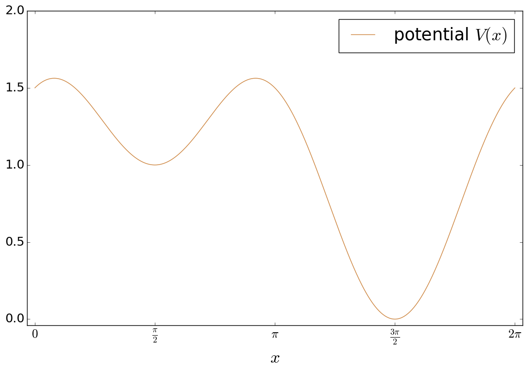
Figure 2: An example of a smooth potential $V$.

The advection term in (1.1) involves a potential $V$ that the particle tries to minimise. To gain some intuition about the action of this term, consider the one-dimensional potential shown in Fig. 2. We expect that, as $t\to\infty$, a particle prefers to sit inside the wells of the potential around $\frac{\pi}{2}$ and $\frac{3\pi}{2}$; indeed, if $K=0$ in (1.1), then solutions to the resulting transport equation would concentrate around these points.

The distribution functions Fig. 1 suggests that for smaller $\beta$, the particle is more likely to make large jumps, as the tails of the distribution are heavier. In turn, this suggests that the particle may be more likely to escape from the minima of the potential $V$ and escape into a higher-energy minimum. It turns out this intuition is indeed borne out by numerical simulation: in Fig. 3, we illustrate how the diffusion process affects the stable-state solution $u_{\infty}$. Fig. 4 shows the evolution of the solution from an initial condition, assuming the particle is initially uniformly distributed close to the less favourable local minimum.

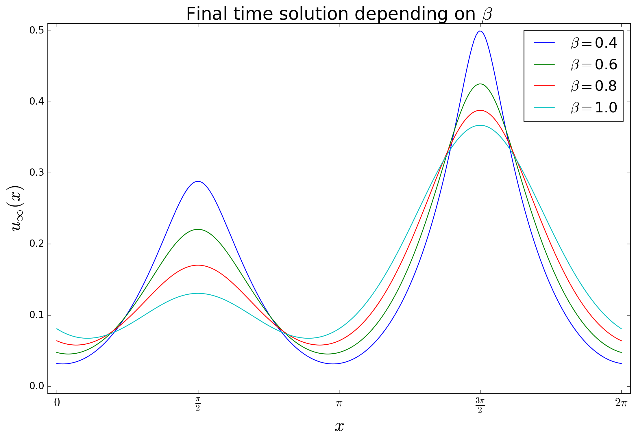
Figure 3: Dependence of final time solution on $\beta$

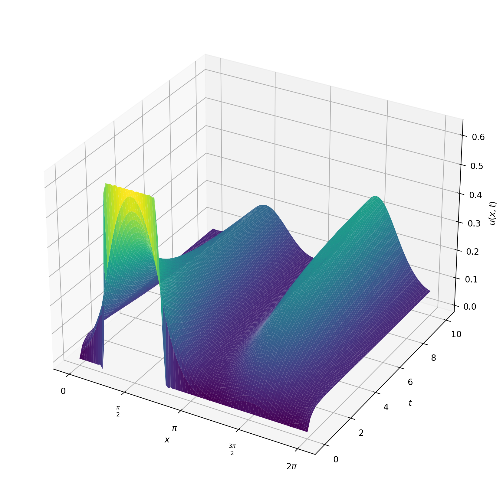
Figure 4: A solution for $\alpha=\beta=0.8$

1.1 Main results

The first of our main results is to establish well-posedness of a mild generalisation of (1.1), where we allow the potential $V$ to depend on time and introduce a source term $f$ on the right-hand side of the equation, allowing sources and sinks. In this context, we aim to find a weak solution with the initial condition given by $u(x,0)=h(x)$ for some given $h$. In other words, we seek $u:\mathbb{T}^{d}\times[0,T]\to\mathbb{R}$ satisfying

$$\int_{\mathbb{T}^{d}}\left(\frac{\partial^{\alpha}u}{\partial t^{\alpha}}+K(-\Delta)^{\beta}u-\nabla\cdot\big{(}\nabla Vu\big{)}\right)v\,\mathrm{d}x =\int_{\mathbb{T}^{d}}fv\,\mathrm{d}x \text{ in }\mathbb{T}^{d}\times(0,T)$$ (1.2)

$$u =h \text{ on }\mathbb{T}^{d}\times\{0\}$$

for every $v\in L^{2}(\mathbb{T}^{d})$. Here, $K>0$ is a positive constant, $V:\mathbb{T}^{d}\times[0,T]\to\mathbb{R}$ a time-dependent potential and $f:\mathbb{T}^{d}\times[0,T]\to\mathbb{R}$ is a source term, and we will require $\alpha\in(0,1]$ and $\beta>\frac{1}{2}$. Later, we will assume that

$$\int_{\mathbb{T}^{d}}f(x,t)\,\mathrm{d}x=0$$ (1.3)

for almost every $t\in[0,T]$. Intuitively-speaking, this means that $f$ only redistributes mass, but does not add or remove any, and is a standard assumption required to make sense of the equation in the periodic setting. This requirement is used to justify Remark 2.4, so that we do not have to worry about the $(u)$ term in the statement of Poincaré’s inequality in the following analysis. However, the assumption (1.3) can probably be dropped and replaced by an estimate on the growth of $|(u)|$ in time depending on $f$, if one is willing to include an additional term in all the following computations.

The main goal of this work is to show the following theorem:

Theorem 1.1.

Suppose $\beta>\frac{1}{2}$, and $V$, $f$ and $h$ are sufficiently regular. Then there is a unique solution $u:\mathbb{T}^{d}\times[0,T]\to\mathbb{R}$ satisfying (1.2). Furthermore, the solution $u$ is sufficiently regular to make sense of $\frac{\partial^{\alpha}u}{\partial t^{\alpha}}$, $(-\Delta)^{{\beta}}u$ and $\nabla u$ for almost every time $t$.

What “sufficiently regular” in each case means is made precise in the statements of Theorem 3.4 and Theorem 4.4.

The methods we use depend centrally on the assumption $\beta>\frac{1}{2}$ and the fact that the equation is considered on a periodic domain $\mathbb{T}^{d}$. The former assumption ensures that the order of differentiation of the fractional Laplacian dominates the forcing term involving $V$, so that the equation remains of parabolic type. The latter assumption allows us to work with Fourier series to simplify many expressions. However, we do observe that some statements for $\beta=\frac{1}{2}$ are also valid, and the numerical scheme we use appears to converge to a reasonable solution even for $\beta<\frac{1}{2}$, given that $\beta$ stays away from $0$, so it may be that our results generalise further.

The main novelty of this work is dealing with the two fractional differential operators in establishing the tools to prove the existence and uniqueness of solutions to the system (1.2) in Section 3. The paper is structured as follows: Section 2 contains several relatively self-contained subsections, establishing prerequisites for the main results. Most notably, Theorem 2.15 generalises a fundamental result in the analysis of elliptic equations to the case of the fractional Laplacian. Furthermore, Theorem 2.21, the main result from [2], replaces a bound usually established using the Leibniz rule, which is unavailable for the Caputo fractional derivative. Section 3 and Section 4 show the existence, uniqueness and some regularity of a solution to (1.2), given some regularity assumptions on $V$, $f$ and $h$. Theorems 3.1, 3.2, 3.4, 3.5 and 4.4 adapt theorems found in Chapter 7 of [3]. The regularity result in Theorem 4.4 is then used to show the $L^{2}$-convergence of numerically computable approximations to the solution, providing a numerical scheme that was also used to create the plots in this paper.

2 Preliminaries

Our main goal is to prove the existence of solutions to (2.11). First, we will find approximate solutions in lower-dimensional subspaces. Then, we prove bounds on these approximations that we can use to pass to a limit to find a full solution. This strategy requires many prerequisite results that are collected in this section.

2.1 Fourier series

We fix a dimension $d\in\mathbb{Z}_{>0}$ and define $\mathbb{T}:=\mathbb{R}/(2\pi\mathbb{Z})$ to be the one-dimensional periodic domain; recall that we consider the PDE on $\mathbb{T}^{d}$. For $k\in\mathbb{Z}^{d}$, define $w_{k}:\mathbb{T}^{d}\to\mathbb{C}$ by

$$w_{k}(x):=\frac{1}{(2\pi)^{d/2}}\mathrm{e}^{ik\cdot x}.$$

We note that $\{w_{k}\}_{k\in\mathbb{Z}^{d}}$ is an orthonormal basis of $L^{2}(\mathbb{T}^{d},\mathbb{C})$; for convenience, we denote this space as $L^{2}:=L^{2}(\mathbb{T}^{d},\mathbb{C})$.

Given a function $u\in L^{2}$, we define the Fourier coefficients of $u$ to be

$$\mathcal{F}\left[u\right](k)=\hat{u}(k)=\left\langle u,w_{k}\right\rangle_{L^{2}}=\int_{\mathbb{T}^{d}}u(x)\overline{w_{k}(x)}\,\mathrm{d}x=\frac{1}{(2\pi)^{d/2}}\int_{\mathbb{T}^{d}}u(x)\mathrm{e}^{-ik\cdot x}\,\mathrm{d}x,$$

for any $k\in\mathbb{Z}^{d}$, and then we have that

$$u(x)=\sum_{k\in\mathbb{Z}^{d}}\hat{u}(k)w_{k}(x),$$

with the equality in $L^{2}$ [10, p22]. Finally, the following result will allow us to move freely from equations in $L^{2}$ to equations in the Fourier space $l^{2}:=l^{2}(\mathbb{Z}^{d},\mathbb{C})$.

Proposition 2.1 (Parseval’s identity).

For any function $u$, it holds that

$$\left\|u\right\|_{L^{2}}=\left\|\hat{u}\right\|_{l^{2}}.$$

In particular, $u\in L^{2}$ if and only if $\hat{u}\in l^{2}$.

2.2 Fractional Sobolev Spaces

Fix $\beta>0$. We focus on the case where $\beta\leq 1$, but this restriction is not necessary. For our purposes, the following definition of the fractional Laplacian as a Fourier multiplier is most convenient [7, p7]:

Definition 2.2 (Fractional Laplacian).

If $\beta>0$ and $u\in L^{2}$, then the Fractional Laplacian of $u$ of order $\beta$ is identified with the pseudodifferential operator defined by the Fourier multiplier $-|k|^{2\beta}$, that is,

$$-(-\Delta)^{{\beta}}u=\mathcal{F}^{-1}\left[-|k|^{2\beta}\mathcal{F}[u](k)\right]$$ (2.1)

whenever the sum $\sum_{k\in\mathbb{Z}^{d}}|k|^{2\beta}\hat{u}(k)$ is finite.

Equipped with this notion, we want to find the right space to look for solutions in. We start by defining the fractional Sobolev space

$$H^{\beta}:=H^{\beta}(\mathbb{T}^{d},\mathbb{C}):=\left\{u\in L^{2}(\mathbb{T}^{d},\mathbb{C}):\left\|(-\Delta)^{{\beta/2}}u\right\|_{L^{2}}<\infty\right\},$$ (2.2)

equipped with the norm

$$\left\|u\right\|_{H^{\beta}}:=\left(\left\|(-\Delta)^{{\beta/2}}u\right\|_{L^{2}}^{2}+\left\|u\right\|_{L^{2}}^{2}\right)^{\frac{1}{2}}.$$ (2.3)

In the case $\beta=1$, this definition aligns with the usual definition of the space of periodic functions

$$H^{1}:=\left\{u\in L^{2}(\mathbb{T}^{d},\mathbb{C}):\left\||\nabla u|\right\|_{L^{2}}<\infty\right\},$$ (2.4)

since

$$\left\|(-\Delta)^{{1/2}}u\right\|_{L^{2}}^{2}=\sum_{k\in\mathbb{Z}^{d}}|k|^{2}|\hat{u}(k)|^{2}=\left\||\nabla u|\right\|_{L^{2}}^{2}.$$ (2.5)

For our analysis, it will be vital that we can bound lower-order derivatives by higher-order derivatives. The following result provides an appropriate version of Poincaré’s inequality to do this.

Proposition 2.3 (Poincaré’s inequality).

1. Suppose $\beta>0$; then for any $u\in H^{\beta}$ we have

   $$\left\|u-(u)\right\|_{L^{2}}\leq\left\|(-\Delta)^{{\beta/2}}u\right\|_{L^{2}},$$ (2.6)

   where

   $$(u):=\mathchoice{{\vbox{\hbox{$\textstyle-$ }}\kern-7.83337pt}}{{\vbox{\hbox{$\scriptstyle-$ }}\kern-5.90005pt}}{{\vbox{\hbox{$\scriptscriptstyle-$ }}\kern-4.75003pt}}{{\vbox{\hbox{$\scriptscriptstyle-$ }}\kern-4.25003pt}}\!\int_{\mathbb{T}^{d}}u(x,t)\,\mathrm{d}x$$

   is the average of $u$ over $\mathbb{T}^{d}$.

2. Suppose $0<\gamma\leq\beta$. Then for any $u\in H^{\beta}$,

   $$\left\|(-\Delta)^{{\gamma/2}}u\right\|_{L^{2}}\leq\left\|(-\Delta)^{{\beta/2}}u\right\|_{L^{2}}.$$

Proof.

Using Proposition 2.1 (Parseval’s identity), we can express (2.6) into the following statement about Fourier coefficients:

$$\left\|u-(u)\right\|_{L^{2}}^{2}=\sum_{k\in\mathbb{Z}^{d}\setminus\{0\}}|\hat{u}(k)|^{2}\leq\sum_{k\in\mathbb{Z}^{d}}|k|^{\beta}|\hat{u}(k)|^{2}=\left\|(-\Delta)^{{\beta/2}}u\right\|_{L^{2}}^{2}.$$

We note that subtracting the average $(u)$ in (2.6) yields the fact that the $k=0$ term in the sum is zero. The second inequality follows by a similar argument. ∎

The appearance of the average $(u)$ in (2.6) (and the fact from Theorem 2.9 that we will establish later that the mass of a function $u$ satisfying the weak PDE is constant in time) motivates working in a space of functions $u$ of constant mass $(u)=0$. Thus, define $\mathcal{H}^{\beta}$ to be the closure of the the subspace

$$\mathcal{H}^{\beta}:=\overline{\{u\in C^{\infty}(\mathbb{T}^{d}):(u)=0\}}^{H^{\beta}}$$

in the Hilbert space $H^{\beta}$ with its corresponding norm.

Remark 2.4.

The function $u\mapsto\left\|(-\Delta)^{{\beta/2}}u\right\|_{L^{2}}$ is a seminorm on $H^{\beta}$; on the other hand, due to the constraint that $(u)=0$, it is a norm on $\mathcal{H}^{\beta}$ that we could use instead. However, there is no need since Proposition 2.3 (Poincaré’s inequality) implies that on $\mathcal{H}^{\beta}$, the norms $\left\|(-\Delta)^{{\beta/2}}\,\cdot\,\right\|_{L^{2}}$ and $\left\|\,\cdot\,\right\|_{H^{\beta}}$ are equivalent.

2.3 The fractional time derivative

Let us turn our attention to the Caputo derivative in the time variable. Given a function $\varphi\in L^{1}([0,T],\mathbb{R})$, we define its fractional integral $I^{\alpha}\varphi(t)$ of order $\alpha>0$ to be [6, p69]

$$I^{\alpha}\varphi(t):=\frac{1}{\Gamma(\alpha)}\int_{0}^{t}(t-\tau)^{\alpha-1}\varphi(\tau)\,\mathrm{d}\tau.$$ (2.7)

If instead $\varphi$ takes values in an arbitrary separable Banach space $X$ and we require $\varphi$ to be an element of the Bochner space $L^{1}([0,T],X)$, the fractional integral $I^{\alpha}\varphi(t)$ can be defined in the same way via Bochner integration.

Using this definition to fractionally integrate in time, we then differentiate to give the following definition for a fractional derivative.

Definition 2.5 (Caputo fractional derivative).

See [8, p78ff]. Let $\alpha\in(0,1)$. Let $X$ be a separable Banach space and $\varphi\in C([0,T],X)$ such that $I^{1-\alpha}\varphi$ is absolutely continuous. Then the Caputo fractional derivative of $\varphi$ is defined to be

$$\frac{\mathrm{d}^{\alpha}\varphi}{\mathrm{d}t^{\alpha}}:=\frac{\mathrm{d}^{\!\!\;}}{\mathrm{d}t^{\!\!\;}}\bigl{(}I^{1-\alpha}(\varphi(t)-\varphi(0))\bigr{)}.$$

Remark 2.6.

A corollary of Morrey’s inequality is that the space of absolutely continuous functions $AC([0,T],X)$ is precisely the Sobolev space $W^{1,1}([0,T],X)$. Thus, requiring a function $\varphi$ to be absolutely continuous is the same as asking for its first weak derivative to exist [2, p676].

Observe that in the above definition, we require $\varphi$ to be continuous only to make sense of $\varphi(0)$. A priori, we would like to be able to take the Caputo fractional derivative of $L^{1}$-functions. Thus, in the following, we will establish a notion of making sense of $\varphi(0)$, motivated by the Lebesgue differentiation theorem.

Theorem 2.7 (A version of the Lebesgue differentiation theorem).

A special case of Proposition 2.10 in [4, p93]. Suppose $X$ is a separable Banach space and $\varphi\in L^{1}([0,T],X)$. Then we have that almost every $t\in[0,T]$ is a Lebesgue point of $\varphi$, that is,

$$\lim_{\varepsilon\to 0}\mathchoice{{\vbox{\hbox{$\textstyle-$ }}\kern-7.83337pt}}{{\vbox{\hbox{$\scriptstyle-$ }}\kern-5.90005pt}}{{\vbox{\hbox{$\scriptscriptstyle-$ }}\kern-4.75003pt}}{{\vbox{\hbox{$\scriptscriptstyle-$ }}\kern-4.25003pt}}\!\int_{B_{\varepsilon}(t)}\left\|\varphi(\tau)-\varphi(t)\right\|_{X}\,\mathrm{d}\tau=0.$$ (2.8)

Notice that the conclusion of Theorem 2.7 holds for every $t\in[0,T]$ if $\varphi$ is continuous as a consequence of the integral mean value theorem. Furthermore, the theorem guarantees that reassigning values of $\varphi$ according to (2.9) does not change the function in $L^{1}([0,T],X)$. This means that it is reasonable to define

$$\varphi(0):=\lim_{\varepsilon\to 0}\int_{0}^{T}\varphi(\tau)\eta_{\varepsilon}(\tau)\,\mathrm{d}\tau,$$ (2.9)

where

$$\eta_{\varepsilon}(t)=\frac{1}{\varepsilon}\mathbf{1}_{[0,\varepsilon)}(t).$$ (2.10)

Choosing $\varphi(0)$ in this way corresponds to choosing the precise representative of the $L^{1}$-functions (see [11, p138ff]). We now have a way compatible with the remaining analysis to compute the Caputo fractional derivative of a function $\varphi\in L^{1}([0,T],X)$ that is not necessarily continuous at $0$, as long as $I^{1-\alpha}\varphi$ is absolutely continuous.

2.4 Weak formulation

Let us return to the equation (1.2). We seek a weak formulation of this equation. As such, we seek to pass part of the fractional Laplacian of $u$ onto a test function $v$.

Lemma 2.8 (Divergence Theorem for the Fractional Laplacian).

For any $\beta,\beta^{\prime}>0$ s.t. we have that

$$\int_{\mathbb{T}^{d}}(-\Delta)^{{\beta}}u\,(-\Delta)^{{\beta^{\prime}}}v\,\mathrm{d}x=\int_{\mathbb{T}^{d}}u(-\Delta)^{{\beta+\beta^{\prime}}}v\,\mathrm{d}x,$$

whenever $u\in H^{\beta}$ and $v\in H^{\beta+\beta^{\prime}}$.

Proof.

First, suppose that $u=w_{k}$ and $v=w_{l}$, where $l,k\in\mathbb{Z}^{d}$. Then

$$\int_{\mathbb{T}^{d}}(-\Delta)^{{\beta}}w_{k}(-\Delta)^{{\beta^{\prime}}}w_{l}\,\mathrm{d}x=|k|^{\beta}|l|^{\beta^{\prime}}\left\langle w_{k},w_{l}\right\rangle_{L^{2}}.$$

This inner product is zero unless $k=l$, and if $k=l$, then $|k|^{\beta}|l|^{\beta^{\prime}}=|l|^{\beta+\beta^{\prime}}$. As such,

$$\int_{\mathbb{T}^{d}}(-\Delta)^{{\beta}}w_{k}(-\Delta)^{{\beta^{\prime}}}w_{l}\,\mathrm{d}x=|l|^{\beta+\beta^{\prime}}\left\langle w_{k},w_{l}\right\rangle_{L^{2}}=\int_{\mathbb{T}^{d}}w_{k}(-\Delta)^{{\beta+\beta^{\prime}}}w_{l}\,\mathrm{d}x.$$

By linearity, the result holds for $u,v\in\mathrm{span}\left(\{w_{k}\}_{k}\right)$, but this space is dense in the corresponding Sobolev spaces $H^{\beta}$ and $H^{\beta+\beta^{\prime}}$, so by continuity, we deduce the result. ∎

In light of the previous result, we define a bilinear form $B:H^{\beta}\times H^{\beta}\to\mathbb{R}$ as

$$B[u,v]:=\int_{\mathbb{T}^{d}}K(-\Delta)^{{\beta/2}}u(-\Delta)^{{\beta/2}}v+(u\nabla V)\cdot\nabla v\,\mathrm{d}x.$$

With this definition, and applying the usual Divergence Theorem along with Lemma 2.8, we propose the following weak formulation of (1.2). We seek a function $u$ satisfying

$$\Bigl{\langle}\frac{\partial^{\alpha}u}{\partial t^{\alpha}},v\Bigr{\rangle}_{L^{2}}+B[u,v] =\left\langle f,v\right\rangle_{L^{2}} \text{ on }\mathbb{T}^{d}\text{ for a.e. }t\in(0,T)$$ (2.11)

$$u =h \text{ on }\mathbb{T}^{d}\text{ for }t=0$$

for any $v\in\mathcal{H}^{\beta}$.

Let us obtain a version of (2.11) in terms of the Fourier transform $\hat{u}$. Observe that the Fourier coefficients of a product is the convolution of the Fourier coefficients, that is,

$$\mathcal{F}\left[\varphi\phi\right]=\hat{\varphi}*\hat{\phi},$$

where $*$ denotes the discrete convolution:

$$\big{(}\hat{\varphi}*\hat{\phi}\big{)}(k)=\sum_{k^{\prime}\in\mathbb{Z}^{d}}\hat{\varphi}(k-k^{\prime})\hat{\phi}(k^{\prime}).$$

Then for $v=w_{k}$, where $k\in\mathbb{Z}^{d}$, (2.11) transforms into

$$\frac{\partial^{\alpha}}{\partial t^{\alpha}}\hat{u}(k,t)+K|k|^{\beta}\hat{u}(k,t)-ik\cdot\left(\mathcal{F}\left[\nabla V\right]*\hat{u}(\cdot,t)\right)=\hat{f}(k,t).$$ (2.12)

Observe that (1.3) precisely means that $\hat{f}(0,t)=0$. In particular, if we take $k=0$, (2.12) trivially shows that $\frac{\partial^{\alpha}}{\partial t^{\alpha}}\hat{u}(0,t)=0$, summarised in the following theorem:

Theorem 2.9 (Conservation of mass).

If $u$ is a weak solution to (1.2), where $\int_{\mathbb{T}^{d}}f(x,t)\,\mathrm{d}x=0$ for a.e. $t$, then the total mass $\int_{\mathbb{T}^{d}}u(x,t)\,\mathrm{d}x$ is constant in time.

Next, let us shift our perspective to the solution $u$. Define $\mathcal{H}^{-\beta}:=\left(\mathcal{H}^{\beta}\right)^{*}$ to be the topological dual of $\mathcal{H}^{\beta}$. We note that

• $\mathcal{H}^{\beta}\subset L^{2}\subset\mathcal{H}^{-\beta}$ are all separable Hilbert spaces; and

• The fractional Sobolev space $\mathcal{H}^{\beta}$ is dense in $L^{2}$, and the embedding given by the identity map is continuous since $\left\|u\right\|_{L^{2}}\leq\left\|u\right\|_{H^{\beta}}$ for all $u\in\mathcal{H}^{\beta}$.

These observations mean that $\mathcal{H}^{\beta}\subset L^{2}\subset\mathcal{H}^{-\beta}$ is a Gel’fand triple, which suggests that we look for solutions of the following form. Define $\mathbf{u}:[0,T]\to\mathcal{H}^{\beta}$ by

$$\mathbf{u}(t):=u(\cdot,t).$$

Given that we expect some regularity in time, we expect $\mathbf{u}$ to be an element of the Bochner space $L^{2}([0,T],\mathcal{H}^{\beta})$. Similarly, let us define $\mathbf{V},\mathbf{f}\in L^{2}([0,T],L^{2})$ by

$$\mathbf{V}(t):=V(\cdot,t)\quad\text{and}\quad\mathbf{f}(t):=f(\cdot,t).$$

We note that we will later require that $\mathbf{V}$ and $\mathbf{f}$ are elements of Bochner spaces with stronger regularity.

Now suppose that $w\in L^{2}\subset\mathcal{H}^{-\beta}$ and $v\in\mathcal{H}^{\beta}$. Then we have

$$\left\langle w,v\right\rangle_{\mathcal{H}^{-\beta},\mathcal{H}^{\beta}}=\left\langle w,v\right\rangle_{L^{2}},$$ (2.13)

(see for example equation (7.14) in [9]) where $\left\langle w,v\right\rangle_{\mathcal{H}^{-\beta},\mathcal{H}^{\beta}}$ is the $\mathcal{H}^{-\beta}$–$\mathcal{H}^{\beta}$ pairing, applying $w$ to $v$. From this point of view, let $\mathbf{u}^{(\alpha)}$ be the Caputo fractional derivative of $\mathbf{u}$ of order $\alpha$. The weak formulation (2.11) can then be read as

$$\left\langle\mathbf{u}^{(\alpha)}(t),v\right\rangle_{L^{2}}=\left\langle\mathbf{f}(t),v\right\rangle_{L^{2}}-B[\mathbf{u}(t),v]\quad\text{for a.e. }t\in(0,T).$$

The right-hand side is a linear functional on $v\in\mathcal{H}^{\beta}$, and this suggests that we can interpret the left-hand side as the pairing $\left\langle\mathbf{u}^{(\alpha)},v\right\rangle_{\mathcal{H}^{-\beta},\mathcal{H}^{\beta}}$ applying $\mathbf{u}^{(\alpha)}$ to $v\in\mathcal{H}^{\beta}$. Thus, it is reasonable to look for a solution $\mathbf{u}\in L^{2}([0,T],\mathcal{H}^{\beta})$ whose Caputo fractional derivative of order $\alpha$ is $\mathbf{u}^{(\alpha)}\in L^{2}([0,T],\mathcal{H}^{-\beta})$.

With these considerations in mind, Section 3 and the remainder of Section 2 establish the existence (and uniqueness) of a solution $\mathbf{u}\in L^{2}([0,T],\mathcal{H}^{\beta})$ with $\mathbf{u}^{(\alpha)}\in L^{2}([0,T],\mathcal{H}^{-\beta})$ such that

$$\left\langle\mathbf{u}^{(\alpha)},v\right\rangle_{L^{2}}+B[\mathbf{u},v] =\left\langle f,v\right\rangle_{L^{2}} \text{ for a.e. }t\in(0,T)$$ (2.14)

$$\mathbf{u}(0) =h$$ in the sense of (2.9)

for any $v\in\mathcal{H}^{\beta}$.

2.5 A coercivity bound

This subsection works towards establishing a priori bounds on weak solutions $\mathbf{u}$, which are encoded in Theorem 2.15. The arguments are a generalisation of standard arguments for elliptic differential operators to the fractional case, but for completeness, we record the details.

Lemma 2.10 (A Young-type inequality).

Suppose $0\leq\beta^{\prime\prime}<\beta^{\prime}<\beta$ and fix $\varepsilon>0$. Then there exists a constant $c(\varepsilon)$ such that for any $u\in\mathcal{H}^{\beta}$,

$$\left\|(-\Delta)^{{\beta^{\prime}}}u\right\|_{L^{2}}^{2}\leq\varepsilon\left\|(-\Delta)^{{\beta}}u\right\|_{L^{2}}^{2}+c(\varepsilon)\left\|(-\Delta)^{{\beta^{\prime\prime}}}u\right\|_{L^{2}}^{2}.$$ (2.15)

We will argue inductively, iteratively splitting the $\beta^{\prime}$-term into a $(\beta^{\prime}+\delta)$- and $(\beta^{\prime}-\delta)$-term, until we hit $\beta^{\prime\prime}$. To keep the coefficient of the $\beta$-term arbitrarily small, we need the following Cauchy Young-type inequality [3, p708]: For $a,b\in\mathbb{R}$ and any $\varepsilon>0$ we have that

$$ab\leq\varepsilon a^{2}+\frac{b^{2}}{4\varepsilon}.$$ (2.16)

Proof.

Define $\delta=\min\{\beta-\beta^{\prime},\beta^{\prime}-\beta^{\prime\prime}\}$. We first use Proposition 2.1 to rewrite the expressions in Fourier space and then use (2.16) to obtain the estimate

$$\left\|(-\Delta)^{{\beta^{\prime}}}u\right\|_{L^{2}}^{2} =\sum_{k}|\hat{u}(k)||k|^{2(\beta^{\prime}+\delta)}|\hat{u}(k)||k|^{2(\beta^{\prime}-\delta)}$$ (2.17)

$$\leq\sum_{k}\frac{\varepsilon}{2}|\hat{u}(k)|^{2}|k|^{4(\beta^{\prime}+\delta)}+\frac{1}{2\varepsilon}|\hat{u}(k)|^{2}|k|^{4(\beta^{\prime}-\delta)}$$

$$=\frac{\varepsilon}{2}\left\|(-\Delta)^{{\beta^{\prime}+\delta}}u\right\|_{L^{2}}^{2}+\frac{1}{2\varepsilon}\left\|(-\Delta)^{{\beta^{\prime}-\delta}}u\right\|_{L^{2}}^{2}.$$

If $\beta^{\prime}-\delta=\beta^{\prime\prime}$, we can employ Proposition 2.3 (Poincaré’s inequality) to estimate

$$\frac{\varepsilon}{2}\left\|(-\Delta)^{{\beta^{\prime}+\delta}}u\right\|_{L^{2}}^{2}\leq\frac{\varepsilon}{2}\left\|(-\Delta)^{{\beta}}u\right\|_{L^{2}}^{2},$$

and we are done. Otherwise, we must have that $\beta^{\prime}+\delta=\beta$, and we can the same argument to the second term on the right-hand side of (2.17), replacing $\beta^{\prime}$ by $\beta^{\prime}-\delta$ and $\varepsilon$ by $\frac{\frac{\varepsilon}{2}}{\frac{1}{2\varepsilon}}=\varepsilon^{2}$. Note that $\delta$ will increase linearly at each step until we reach the first case, and so by repeating the argument inductively as needed, we arrive at the desired estimate. ∎

The following proposition is the key step in the proof of Theorem 2.15. It also provides some control over all of the constants in the bound on the forcing term and allows for $\beta=\frac{1}{2}$, which makes it a useful result by itself.

Proposition 2.11 (Weak bound on the forcing term).

Suppose the potential $V$ is regular enough to ensure that the constant

$$c(V):=\frac{1}{(2\pi)^{d/2}}\Big{(}\left\|\mathcal{F}\left[\nabla V\right]\right\|_{l^{1}}+\left\|\mathcal{F}\left[(-\Delta)^{{3/4}}V\right]\right\|_{l^{1}}\Big{)}$$ (2.18)

is finite, and suppose that $u,v\in\mathcal{H}^{\beta}$, where $\beta\geq\frac{1}{2}$; then

$$(2\pi)^{d/2}\left|\int_{\mathbb{T}^{d}}\nabla Vu\cdot\nabla v\,\mathrm{d}x\right| \leq\left\|\mathcal{F}\left[\nabla V\right]\right\|_{l^{1}}\left\|(-\Delta)^{{1/4}}u\right\|_{L^{2}}\left\|(-\Delta)^{{1/4}}v\right\|_{L^{2}}$$ (2.19)

$$\hskip 56.9055pt+\left\|\mathcal{F}\left[(-\Delta)^{{3/4}}V\right]\right\|_{l^{1}}\left\|u\right\|_{L^{2}}\left\|(-\Delta)^{{1/4}}v\right\|_{L^{2}},$$

and in particular,

$$\left|\int_{\mathbb{T}^{d}}\nabla Vu\cdot\nabla v\,\mathrm{d}x\right|\leq c(V)\left\|(-\Delta)^{{1/4}}u\right\|_{L^{2}}\left\|(-\Delta)^{{1/4}}v\right\|_{L^{2}}.$$ (2.20)

Proof.

We will prove the inequality in Fourier space. Thus, we first need to transform the forcing term in terms of $V$, $u$ and $v$ into an expression involving $\hat{V}$, $\hat{u}$ and $\hat{v}$. Hence, we compute

$$\int_{\mathbb{T}^{d}}u\nabla V\cdot\nabla v\,\mathrm{d}x =\sum_{j=1}^{d}\int_{\mathbb{T}^{d}}u\frac{\partial^{\!\!\;}V}{\partial x_{j}^{\!\!\;}}\frac{\partial^{\!\!\;}v}{\partial x_{j}^{\!\!\;}}\,\mathrm{d}x$$ (2.21)

$$=\sum_{j=1}^{d}\int_{\mathbb{T}^{d}}\sum_{l\in\mathbb{Z}^{d}}\hat{V}(l)il_{j}w_{l}\sum_{m\in\mathbb{Z}^{d}}\hat{u}(m)w_{m}\sum_{k\in\mathbb{Z}^{d}}\hat{v}(k)ik_{j}w_{k}\,\mathrm{d}x$$

$$=-\frac{1}{(2\pi)^{d/2}}\sum_{\begin{subarray}{c}k,l,m\in\mathbb{Z}^{d}\\ k+l+m=0\end{subarray}}\hat{V}(l)\hat{u}(m)\hat{v}(k)l\cdot k,$$

where $\cdot$ is the standard vector dot product.

Let us start by noting that

$$\sum_{k\in\mathbb{Z}^{d}}\left|\hat{u}(-l-k)\right|^{2}|k|=\sum_{m\in\mathbb{Z}^{d}}\left|\hat{u}(m)\right|^{2}|-m-l|\leq\sum_{m\in\mathbb{Z}^{d}}\left|\hat{u}(m)\right|^{2}|m|+|l|\sum_{m\in\mathbb{Z}^{d}}\left|\hat{u}(m)\right|^{2}.$$

Thus, applying the Cauchy-Schwarz inequality and the inequality just derived, we obtain

$$\left|\sum_{k\in\mathbb{Z}^{d}}\hat{u}(-l-k)\hat{v}(k)k\right|$$ (2.22)

$$\qquad\leq\sum_{k\in\mathbb{Z}^{d}}\left|\hat{u}(-l-k)|k|^{\frac{1}{2}}\right|\left|\hat{v}(k)|k|^{\frac{1}{2}}\right|$$

$$\qquad\leq\bigg{(}\sum_{k\in\mathbb{Z}^{d}}\left|\hat{u}(-l-k)\right|^{2}|k|\bigg{)}^{\frac{1}{2}}\bigg{(}\sum_{k\in\mathbb{Z}^{d}}\left|\hat{v}(k)\right|^{2}|k|\bigg{)}^{\frac{1}{2}}$$

$$\qquad\leq\bigg{(}\sum_{k\in\mathbb{Z}^{d}}\left|\hat{u}(k)\right|^{2}|k|+|l|\sum_{k\in\mathbb{Z}^{d}}\left|\hat{u}(k)\right|^{2}\bigg{)}^{\frac{1}{2}}\bigg{(}\sum_{k\in\mathbb{Z}^{d}}\left|\hat{v}(k)\right|^{2}|k|\bigg{)}^{\frac{1}{2}}$$

$$\qquad\leq\bigg{(}\sum_{k\in\mathbb{Z}^{d}}\left|\hat{u}(k)\right|^{2}|k|\bigg{)}^{\frac{1}{2}}\bigg{(}\sum_{k\in\mathbb{Z}^{d}}\left|\hat{v}(k)\right|^{2}|k|\bigg{)}^{\frac{1}{2}}+|l|^{\frac{1}{2}}\bigg{(}\sum_{k\in\mathbb{Z}^{d}}\left|\hat{u}(k)\right|^{2}\bigg{)}^{\frac{1}{2}}\bigg{(}\sum_{k\in\mathbb{Z}^{d}}\left|\hat{v}(k)\right|^{2}|k|\bigg{)}^{\frac{1}{2}}$$

$$\qquad=\left\|(-\Delta)^{{1/4}}u\right\|_{L^{2}}\left\|(-\Delta)^{{1/4}}v\right\|_{L^{2}}+|l|^{\frac{1}{2}}\left\|u\right\|_{L^{2}}\left\|(-\Delta)^{{1/4}}v\right\|_{L^{2}}.$$

Returning once more to the identity obtained in (2.21) and using the estimate in (2.22), we can bound

$$\left|\sum_{k+l+m=0}\hat{V}(l)\hat{u}(m)\hat{v}(k)l\cdot k\right| \hskip 113.81102pt\leq\sum_{l\in\mathbb{Z}^{d}}\left|\hat{V}(l)l\right|\left|\sum_{k\in\mathbb{Z}^{d}}\hat{u}(-l-k)\hat{v}(k)k\right|$$ (2.23)

$$\leq\sum_{l\in\mathbb{Z}^{d}}\left|\hat{V}(l)\right|\left|l\right|\left\|(-\Delta)^{{1/4}}u\right\|_{L^{2}}\left\|(-\Delta)^{{1/4}}v\right\|_{L^{2}}+\sum_{l\in\mathbb{Z}^{d}}\left|\hat{V}(l)\right||l|^{\frac{3}{2}}\left\|u\right\|_{L^{2}}\left\|(-\Delta)^{{1/4}}v\right\|_{L^{2}}$$

$$=\left\|\mathcal{F}\left[\nabla V\right]\right\|_{l^{1}}\left\|(-\Delta)^{{1/4}}u\right\|_{L^{2}}\left\|(-\Delta)^{{1/4}}v\right\|_{L^{2}}+\left\|\mathcal{F}\left[(-\Delta)^{{3/4}}V\right]\right\|_{l^{1}}\left\|u\right\|_{L^{2}}\left\|(-\Delta)^{{1/4}}v\right\|_{L^{2}}.$$

This completes the proof of (2.19). To yield (2.20), we now apply Proposition 2.3 to $\left\|u\right\|_{L^{2}}$ in (2.23). ∎

Remark 2.12.

The constant $c(V)$ arising from the potential $V$ in the inequalities in Proposition 2.11 are given in terms of the $l^{1}$-norm of the Fourier transform of derivatives of $V$. It would be convenient to compare the $l^{1}$-norm of a function’s Fourier transform directly to the function’s $L^{\infty}$-norm, in other words, to establish an equality up to constants between $\left\|f\right\|_{L^{\infty}}$ and $\|\hat{f}\|_{l^{1}}$. The triangle inequality immediately gives that for $f\in L^{\infty}$,

$$\left\|f\right\|_{L^{\infty}}\leq\|\hat{f}\|_{l^{1}}.$$ (2.24)

However, the reverse inequality is not true, as noted in the discussion about the Hausdorff-Young Theorem, which gives a more general version of (2.24), in [5, p124]. An explicit counterexample is the continuous $2\pi$-periodic function $f(x)=\sum_{n=2}^{\infty}\frac{\mathrm{e}^{in\log n}}{n^{1/2}(\log n)^{2}}\mathrm{e}^{inx}$, which satisfies $\sum_{n}|\hat{f}(n)|=\infty$ [14, p199f].

Remark 2.13.

If $V\in H^{3}$, then the constant $c(V)$ exists. Indeed, then by Proposition 2.1,

$$\sum_{l\in\mathbb{Z}^{d}}\left(\left|\hat{V}(l)\right||l|^{3}\right)^{2}=\left\|\mathcal{F}\left[D^{3}V\right]\right\|_{l^{2}}^{2}=\left\|D^{3}V\right\|_{L^{2}}^{2}<\infty.$$

In particular,

$$\left|\hat{V}(l)\right||l|^{3}\leq C$$

is bounded uniformly in $l$ by some constant $C$ depending on $V$. Hence,

$$\left\|\mathcal{F}\left[(-\Delta)^{{3/4}}V\right]\right\|_{l^{1}}=\sum_{l\in\mathbb{Z}^{d}}|\hat{V}(l)||l|^{\frac{3}{2}}\leq C\sum_{l\in\mathbb{Z}^{d}}\frac{1}{|l|^{\frac{3}{2}}}<\infty,$$ (2.25)

and similarly for $\left\|\mathcal{F}\left[\nabla V\right]\right\|_{l^{1}}$. Observe that this condition can be weakened and merely aims to provide an easier-to-check requirement on $V$.

Proposition 2.14 (Strong bound on the forcing term).

Suppose $V$ is sufficiently regular to guarantee that $c(V)$ defined in (2.18) is finite, $\beta>\frac{1}{2}$ and $u\in\mathcal{H}^{\beta}$. Then, for any $\varepsilon>0$, we have that

$$\left|\int_{\mathbb{T}^{d}}\nabla Vu\cdot\nabla u\,\mathrm{d}x\right|\leq\varepsilon\left\|(-\Delta)^{{\beta/2}}u\right\|_{L^{2}}^{2}+c(V)c(\varepsilon)\left\|u\right\|_{L^{2}}^{2},$$ (2.26)

where the constant $c(\varepsilon)$ is identical to that in the statement of Proposition 2.11.

Proof.

Substitute $v=u$ into (2.20) and employ Lemma 2.10 to conclude

$$\left|\int_{\mathbb{T}^{d}}\nabla Vu\cdot\nabla u\,\mathrm{d}x\right|\leq c(V)\left\|(-\Delta)^{{1/2}}u\right\|_{L^{2}}^{2}\leq\varepsilon\left\|(-\Delta)^{{\beta/2}}u\right\|_{L^{2}}^{2}+c(V)c(\varepsilon)\left\|u\right\|_{L^{2}}^{2}.\qed$$

Finally, we can use (2.26) to show the following key theorem for the bilinear form $B[\cdot,\cdot]$; compare with [3, p320].

Theorem 2.15 (Coercivity bound).

Suppose that $K>0$, $c(V)\leq M_{1}$ for some $M_{1}$, $\beta>\frac{1}{2}$.

1. There exist constants $\gamma_{1}>0$, $\gamma_{2}\geq 0$ depending on $K$, $M_{1}$ and $\beta$ such that

   $$\gamma_{1}\left\|u\right\|_{H^{\beta}}^{2}\leq B[u,u]+\gamma_{2}\left\|u\right\|_{L^{2}}^{2}$$ (2.27)

   for any $u\in\mathcal{H}^{\beta}$.

2. If we make the stronger hypothesis $K>c(V)$ and $\beta\geq\frac{1}{2}$, there is just one constant $\gamma>0$ such that

   $$\gamma\left\|u\right\|_{H^{\beta}}^{2}\leq B[u,u]+\gamma\left\|u\right\|_{L^{2}}^{2}$$ (2.28)

   for any $u\in\mathcal{H}^{\beta}$.

Proof.

By definition,

$$K\int_{\mathbb{T}^{d}}\left|(-\Delta)^{{\beta/2}}u\right|^{2}\,\mathrm{d}x=B[u,u]+\int_{\mathbb{T}^{d}}u\nabla V\cdot\nabla u\,\mathrm{d}x.$$

Choosing $0<\varepsilon<K$ in (2.26), we estimate the second term on the right-hand side above:

$$K\left\|(-\Delta)^{{\beta/2}}u\right\|_{L^{2}}^{2} \leq B[u,u]+\varepsilon\left\|(-\Delta)^{{\beta/2}}u\right\|_{L^{2}}^{2}+c(V)c(\varepsilon)\left\|u\right\|_{L^{2}}^{2}.$$

Rearranging gives

$$\left(K-\varepsilon\right)\left(\left\|u\right\|_{L^{2}}^{2}+\left\|(-\Delta)^{{\beta/2}}u\right\|_{L^{2}}^{2}\right)\leq B[u,u]+\left(K-\varepsilon+M_{1}c(\varepsilon)\right)\left\|u\right\|_{L^{2}}^{2},$$ (2.29)

proving (2.27). For (2.28), we may take $c(V)$ instead of $\varepsilon$ and use the same strategy with the weak bound on the forcing term (2.20). ∎

2.6 Initial results

Later, we will start by finding a sequence $\mathbf{u}_{m}$ of approximate solutions on finite-dimensional subspaces of $\mathcal{H}^{\beta}$. In order to deal with the Caputo fractional derivative, we need the following fractional version of Picard-Lindelöf’s Theorem, which we adapt from Theorem 4.1 and Remark 3.1 in [13].

Theorem 2.16 (Existence and Uniqueness for Fractional Linear ODEs).

If $\alpha\in(0,1]$ and $g:[0,T]\times\mathbb{C}^{n}\to\mathbb{C}^{n}$ is a continuous function which is globally Lipschitz continuous in the $\mathbb{C}^{n}$-variable, then the system

$$\frac{\mathrm{d}^{\alpha}}{\mathrm{d}t^{\alpha}}y(t) =g(t,y(t)),$$ (2.30)

$$y(0) =y_{0}$$

has a unique global solution $y\in C([0,T],\mathbb{C}^{n})$.

We will then need to prove some bounds for these approximate solutions $\mathbf{u}_{m}$ before passing to limits. Grönwall’s inequality is an incredibly powerful tool to find such bounds; however, since we work with a Caputo fractional derivative, we need an adapted version.

Theorem 2.17 (differential version of Grönwall’s inequality for the Caputo fractional derivative).

Suppose that $\alpha\in(0,1]$ and $\varphi\in L^{1}([0,T],\mathbb{R})$ is a nonnegative function s.t. $I^{1-\alpha}\varphi$ is absolutely continuous. Let $c>0$ and suppose $\zeta:[0,T]\to\mathbb{R}$ is a nonnegative nondecreasing integrable function. If

$$\frac{\mathrm{d}^{\alpha}}{\mathrm{d}t^{\alpha}}\varphi(t)\leq c\,\varphi(t)+\zeta(t)$$ (2.31)

for almost every $t\in[0,T]$, then

$$\varphi(t)\leq(I^{\alpha}\zeta(t)+\varphi(0))E_{\alpha}(ct^{\alpha}),$$ (2.32)

where $E_{\alpha}$ is the Mittag-Leffler function defined via the power series

$$E_{\alpha}(z):=\sum_{k=0}^{\infty}\frac{z^{k}}{\Gamma(\alpha k+1)},$$ (2.33)

and $\Gamma(z):=\int_{0}^{\infty}t^{z-1}\mathrm{e}^{-t}\,\mathrm{d}t$ is the usual Gamma function.

Proof.

This is a Corollary of Theorem 8 in [1, p9f]. From Lemma 2.5 (b) in [6, p74f] (also compare Lemma 2.22 in [6, p96]), we conclude that since $I^{1-\alpha}\varphi$ is absolutely continuous by assumption,

$$I^{\alpha}\left(\frac{\mathrm{d}^{\alpha}}{\mathrm{d}t^{\alpha}}\varphi(t)\right)=\varphi(t)-\varphi(0).$$ (2.34)

$I^{\alpha}$ is a monotone linear operator, so applying it to both sides of (2.31) preserves the inequality, yielding

$$\varphi(t)-\varphi(0)\leq cI^{\alpha}\varphi(t)+I^{\alpha}\zeta(t).$$ (2.35)

Since $\zeta$ is assumed to be both nonnegative and nondecreasing, $I^{\alpha}\zeta$ inherits both properties, and we may apply Theorem 8 in [1, p9f] to deduce (2.32). ∎

Once approximate solutions $\mathbf{u}_{m}$ are available, we want to send $m$ to infinity. The following three results relate to the current discussion and enable us to pass properties of $\mathbf{u}_{m}$ to the limit $\mathbf{u}$.

Lemma 2.18 (Preservation of initial condition).

Suppose that

$$\mathbf{u}_{m}\xrightharpoonup{}\mathbf{u}\qquad\text{ weakly in }L^{2}\left([0,T],\mathcal{H}^{\beta}\right),$$ (2.36)

and $\left\langle\mathbf{u}_{m}(0),w\right\rangle_{L^{2}}=\left\langle h,w\right\rangle_{L^{2}}$ for every $w\in\mathrm{span}\left(\{w_{k}\}_{|k|\leq m}\right)$, in the sense of (2.9). Then

$$\mathbf{u}(0)=h$$ (2.37)

again in the sense of (2.9).

Proof.

Given $\varepsilon>0$, recall the definition of $\eta_{\varepsilon}$ from (2.10). Fix an arbitrary $w\in\mathrm{span}\left(\{w_{k}\}_{k\in\mathbb{Z}^{d}}\right)$. Then, passing to weak limits,

$$\int_{0}^{T}\left\langle\mathbf{u}_{m}(t),\eta_{\varepsilon}(t)w\right\rangle_{L^{2}}\,\mathrm{d}t\to\int_{0}^{T}\left\langle\mathbf{u}(t),\eta_{\varepsilon}(t)w\right\rangle_{L^{2}}\,\mathrm{d}t\qquad\text{ as }m\to\infty.$$ (2.38)

Moreover, using (2.9) for fixed $m$, we have

$$\int_{0}^{T}\left\langle\mathbf{u}_{m}(t),\eta_{\varepsilon}(t)w\right\rangle_{L^{2}}\,\mathrm{d}t\to\left\langle\mathbf{u}_{m}(0),w\right\rangle_{L^{2}}=\left\langle h,w\right\rangle_{L^{2}}\qquad\text{ as }\varepsilon\to 0,$$ (2.39)

where the latter equality holds by assumption. Applying the triangle inequality, we may therefore conclude that

$$\int_{0}^{T}\left\langle\mathbf{u}(t),\eta_{\varepsilon}(t)w\right\rangle_{L^{2}}\,\mathrm{d}t\to\left\langle h,w\right\rangle_{L^{2}}\qquad\text{ as }\varepsilon\to 0,$$

and thus by (2.9),

$$\left\langle\mathbf{u}(0),w\right\rangle_{L^{2}}=\left\langle h,w\right\rangle_{L^{2}}.$$

Since $w\in\mathrm{span}\left(\{w_{k}\}_{k\in\mathbb{Z}^{d}}\right)$ is arbitrary and the span (excluding the $k=0$ term) is dense in $\mathcal{H}^{\beta}$, the conclusion follows. ∎

Since we will deal with weak limits at first, we first need to find the right linear functional to consider, given by the following Lemma:

Lemma 2.19 (Bounded linear functional).

For any given $\phi\in C_{c}^{\infty}(0,T)$ and $w\in\mathcal{H}^{\beta}$, we have that $\Phi:L^{2}([0,T],\mathcal{H}^{\beta})\to\mathbb{C}$ defined by

$$\Phi(\mathbf{v}):=\int_{0}^{T}\left\langle I^{1-\alpha}\mathbf{v}(t),\phi^{\prime}(t)w\right\rangle_{L^{2}}\,\mathrm{d}t$$ (2.40)

is a bounded linear functional.

Proof.

Using the fact that $I^{1-\alpha}:L^{2}\to L^{2}$ is a bounded linear operator from Theorem 2.6 in [12, p48], the continuity of the embedding $\mathcal{H}^{\beta}\to L^{2}$ and the Cauchy-Schwarz inequality twice, we know that there is a constant $C$ s.t.

$$\Phi(\mathbf{v}) \leq\int_{0}^{T}\left|\left\langle I^{1-\alpha}\mathbf{v}(t),\phi^{\prime}(t)w\right\rangle_{L^{2}}\right|\,\mathrm{d}t$$

$$\leq\int_{0}^{T}\left\|I^{1-\alpha}\mathbf{v}(t)\right\|_{L^{2}}|\phi^{\prime}(t)|\left\|w\right\|_{L^{2}}\,\mathrm{d}t$$

$$\leq\left\|w\right\|_{L^{2}}\int_{0}^{T}C\left\|\mathbf{v}(t)\right\|_{L^{2}}|\phi^{\prime}(t)|\,\mathrm{d}t$$

$$\leq\left\|w\right\|_{L^{2}}C\left\|\phi^{\prime}\right\|_{L^{2}([0,T])}\left\|\mathbf{v}\right\|_{L^{2}([0,T],\mathcal{H}^{\beta})}.\qed$$

Finally, we need to be able to pass to limits, keeping the relation between the solution and its Caputo fractional derivative.

Proposition 2.20 (Bochner limits).

Compare to Problem 5 of Chapter 7 in [3, p449]. Assume that

$$\mathbf{u}_{m} \xrightharpoonup{}\mathbf{u}\qquad\text{ weakly in }L^{2}\left([0,T],\mathcal{H}^{\beta}\right)$$

$$\mathbf{u}_{m}^{(\alpha)} \xrightharpoonup{}\mathbf{v}\qquad\text{ weakly in }L^{2}\left([0,T],\mathcal{H}^{-\beta}\right).$$

Then $\mathbf{v}=\mathbf{u}^{(\alpha)}$.

Proof.

Let $\phi\in C_{c}^{\infty}(0,T)$ and $w\in\mathcal{H}^{\beta}$ be arbitrary. Then we have, by definition, for every $m$ that

$$\int_{0}^{T}\left\langle\mathbf{u}_{m}^{(\alpha)}(t),\phi(t)w\right\rangle_{\mathcal{H}^{-\beta},\mathcal{H}^{\beta}}\,\mathrm{d}t=-\int_{0}^{T}\left\langle I^{1-\alpha}\big{(}\mathbf{u}_{m}(t)-\mathbf{u}_{m}(0)\big{)},\phi^{\prime}(t)w\right\rangle_{L^{2}}\,\mathrm{d}t.$$ (2.41)

Using Lemma 2.19 on the right-hand side, we may pass to weak limits on both sides to obtain

$$\int_{0}^{T}\left\langle\mathbf{v}(t),\phi(t)w\right\rangle_{\mathcal{H}^{-\beta},\mathcal{H}^{\beta}}\,\mathrm{d}t=-\int_{0}^{T}\left\langle I^{1-\alpha}\big{(}\mathbf{u}(t)-\mathbf{u}(0)\big{)},\phi^{\prime}(t)w\right\rangle_{L^{2}}\,\mathrm{d}t.$$ (2.42)

Since this equation holds for every $w\in\mathcal{H}^{\beta}$, we conclude

$$\int_{0}^{T}\phi(t)\mathbf{v}(t)\,\mathrm{d}t=\int_{0}^{T}\phi(t)\mathbf{u}^{(\alpha)}(t)\,\mathrm{d}t,$$ (2.43)

for every $\phi\in C_{c}^{\infty}(0,T)$, i.e. $\mathbf{v}=\mathbf{u}^{(\alpha)}$. ∎

Before we show the existence of solutions, we need one final important ingredient to replace the Leibnitz rule for integer-order differentiation. Instead of the equality $\frac{\mathrm{d}^{\!\!\;}}{\mathrm{d}t^{\!\!\;}}\left\|\mathbf{u}(t)\right\|_{L^{2}}^{2}=2\left\langle\frac{\mathrm{d}^{\!\!\;}\mathbf{u}}{\mathrm{d}t^{\!\!\;}},\mathbf{u}(t)\right\rangle_{\mathcal{H}^{-\beta},\mathcal{H}^{\beta}}$, we will use the following fractional version, which is taken from Theorem 4.16 part (b) in [2].

Theorem 2.21.

Suppose that $\mathbf{u}\in L^{2}([0,T],\mathcal{H}^{\beta})$, $\mathbf{u}^{(\alpha)}\in L^{2}([0,T],\mathcal{H}^{-\beta})$ and that $I^{1-\alpha}\left\|\mathbf{u}(t)\right\|_{L^{2}}^{2}$ is absolutely continuous. Then after a possible reidentification, we may assume that $\mathbf{u}\in C([0,T],L^{2})$ and

$$\frac{\mathrm{d}^{\alpha}}{\mathrm{d}t^{\alpha}}\left\|\mathbf{u}(t)\right\|_{L^{2}}^{2}\leq 2\left\langle\mathbf{u}^{(\alpha)}(t),\mathbf{u}(t)\right\rangle_{\mathcal{H}^{-\beta},\mathcal{H}^{\beta}}.$$ (2.44)

Remark 2.22.

The issue of defining an initial condition precisely for the purposes of ensuring the fractional Caputo derivative is well-defined is only briefly discussed in [2]. However, we observe that it is a posteriori demonstrated that $u$ is continuous by showing that a reasonable sequence of mollifications of $u$ is Cauchy in $C([0,T],L^{2})$. This means that our choice to define $u(0)$ in the manner given in (2.9) does not violate any steps taken in [2].

3 Existence and uniqueness of weak solutions

The following two subsections, concerning existence and uniqueness, adapt strategies outlined in [3, p377ff] to our fractional differential equation. In particular, Theorems 3.1, 3.2, 3.4 and 3.5 correspond to Theorems 1, 2, 3 and 4 on pages 378–381 of [3], respectively.

3.1 Existence results

Theorem 3.1 (Approximate solutions).

Suppose that all coefficients of the equation are continuous in time, i.e. $\mathbf{V}\in C([0,T],H^{1})$ and $\mathbf{f}\in C([0,T],L^{2})$. Then, for every positive integer $m$ there is a unique function $\mathbf{u}_{m}:\mathbb{T}^{d}\times[0,T]\to\mathbb{R}$ of the form

$$\mathbf{u}_{m}(t)=\sum_{|k|\leq m}d_{m}^{k}(t)w_{k},$$ (3.1)

where the coefficients $d_{m}^{k}(t)$ satisfy

$$d_{m}^{k}(0)=\left\langle h,w_{k}\right\rangle_{L^{2}},$$ (3.2)

solving the weak equation

$$\left\langle\mathbf{u}_{m}^{(\alpha)},w_{k}\right\rangle_{\mathcal{H}^{-\beta},\mathcal{H}^{\beta}}+B[\mathbf{u}_{m},w_{k}]=\left\langle\mathbf{f},w_{k}\right\rangle_{L^{2}}$$ (3.3)

for all times $0\leq t\leq T$ and $|k|\leq m$.

Proof.

Insert (3.1) into the equation given in (3.3). Using the fact from (2.13) that the $\mathcal{H}^{-\beta}$–$\mathcal{H}^{\beta}$ pairing is equivalent to the $L^{2}$ inner product whenever both make sense, we obtain the system of equations in $|k|\leq m$,

$$\frac{\mathrm{d}^{\alpha}}{\mathrm{d}t^{\alpha}}d_{m}^{k}(t)+\sum_{|j|\leq m}B[w_{j},w_{k}]d_{m}^{j}(t)=\mathbf{\hat{f}}(k,t).$$

If we define $g:[0,T]\times\mathbb{C}^{(2m+1)^{d}}\to\mathbb{C}^{(2m+1)^{d}}$, the spaces indexed by $|k|\leq m$, by

$$g_{k}(t,y)=\mathbf{\hat{f}}(k,t)-\sum_{|j|\leq m}B[w_{j},w_{k};t]y_{j},$$

then the equation reads

$$\frac{\mathrm{d}^{\alpha}}{\mathrm{d}t^{\alpha}}d_{m}^{k}(t)=g_{k}\left(t,\bigl{(}d_{m}^{j}(t)\bigr{)}_{|j|\leq m}\right).$$ (3.4)

Since

$$\big{|}\hat{\mathbf{f}}(k,t)-\hat{\mathbf{f}}(k,\tau)\big{|}=\left|\left\langle{\mathbf{f}}(\cdot,t),w_{k}\right\rangle_{L^{2}}-\left\langle{\mathbf{f}}(\cdot,\tau),w_{k}\right\rangle_{L^{2}}\right|\leq\left\|{\mathbf{f}}(\cdot,t)-{\mathbf{f}}(\cdot,\tau)\right\|_{L^{2}}$$

for arbitrary $t$ and $\tau$ and fixed $k$, the assumptions on $\mathbf{V}$ and $\mathbf{f}$ imply that $g$ is continuous on $[0,T]\times\mathbb{C}^{n}$ and Lipschitz in $y$. Then Theorem 2.16 yields that subject to the initial conditions (3.2), the equation (3.4) has a unique continuous solution. ∎

Given the approximate solutions $\mathbf{u}_{m}$, we want to pass to a limit. The next theorem provides the bounds needed and uses many of the results from Section 2. First, suppose that there exists

$$M_{1}:=\sup_{t\in[0,T]}c(\mathbf{V}(t)),$$ (3.5)

where $c(\cdot)$ is the constant defined in (2.18).

Theorem 3.2 (Energy estimates).

Suppose $\beta>\frac{1}{2}$. Assume that the constant in (2.18) exists (see Remark 2.13). Then there exists a constant $C$, depending only on $\alpha$, $\beta$, the final time $T$, the diffusion constant $K$ and the bound $M_{1}$, such that

$$\sup_{0\leq t\leq T}\left\|\mathbf{u}_{m}(t)\right\|_{L^{2}}+\left\|\mathbf{u}_{m}\right\|_{L^{2}\left([0,T],\mathcal{H}^{\beta}\right)}+\left\|\mathbf{u}_{m}^{(\alpha)}\right\|_{L^{2}\left([0,T],\mathcal{H}^{-\beta}\right)}\leq C\left(\left\|h\right\|_{L^{2}}+\left\|\mathbf{f}\right\|_{L^{\infty}([0,T],L^{2})}\right).$$ (3.6)

Proof.

For all $0\leq t\leq T$, we multiply equation (3.3) by $d_{m}^{k}(t)$ and sum over $|k|\leq m$ to find the equation

$$\left\langle\mathbf{u}_{m}^{(\alpha)},\mathbf{u}_{m}\right\rangle_{\mathcal{H}^{-\beta},\mathcal{H}^{\beta}}+B[\mathbf{u}_{m},\mathbf{u}_{m}]=\left\langle\mathbf{f},\mathbf{u}_{m}\right\rangle_{L^{2}}.$$ (3.7)

Combining the Cauchy-Schwarz and Young’s inequality, we have $|\left\langle\mathbf{f},\mathbf{u}_{m}\right\rangle_{L^{2}}|\leq\left\|\mathbf{f}\right\|_{L^{2}}\left\|\mathbf{u}_{m}\right\|_{L^{2}}\leq\frac{1}{2}(\left\|\mathbf{f}\right\|_{L^{2}}^{2}+\left\|\mathbf{u}_{m}\right\|_{L^{2}}^{2})$. Recalling Theorem 2.21, we have that $\frac{\mathrm{d}^{\alpha}}{\mathrm{d}t^{\alpha}}\left(\left\|\mathbf{u}_{m}\right\|_{L^{2}}^{2}\right)\leq 2\left\langle\mathbf{u}_{m}^{(\alpha)},\mathbf{u}_{m}\right\rangle_{\mathcal{H}^{-\beta},\mathcal{H}^{\beta}}$. Thus, we can use (3.7) and (2.27) to estimate

$$\frac{\mathrm{d}^{\alpha}}{\mathrm{d}t^{\alpha}}\left(\left\|\mathbf{u}_{m}\right\|_{L^{2}}^{2}\right)+2\gamma_{1}\left\|\mathbf{u}_{m}\right\|_{H^{\beta}}^{2} \leq 2\left(\gamma_{1}\left\|\mathbf{u}_{m}\right\|_{H^{\beta}}^{2}+\left\langle\mathbf{f},\mathbf{u}_{m}\right\rangle_{L^{2}}-B[\mathbf{u}_{m},\mathbf{u}_{m}]\right)$$ (3.8)

$$\leq(2\gamma_{2}+1)\left\|\mathbf{u}_{m}\right\|_{L^{2}}^{2}+\left\|\mathbf{f}\right\|_{L^{2}}^{2}.$$ (3.9)

Note that the dependency of $\gamma_{1}$ and $\gamma_{2}$ on $c(V)$ in Theorem 2.15 means that we can choose both constants using the uniform bound $M_{1}$ instead of $c(V)$.

In particular, $\frac{\mathrm{d}^{\alpha}}{\mathrm{d}t^{\alpha}}\left(\left\|\mathbf{u}_{m}\right\|_{L^{2}}^{2}\right)\leq(2\gamma_{2}+1)\left\|\mathbf{u}_{m}\right\|_{L^{2}}^{2}+\left\|\mathbf{f}\right\|_{L^{2}}^{2}$, so the differential version of Grönwall’s Lemma in Theorem 2.17 yields

$$\left\|\mathbf{u}_{m}(t)\right\|_{L^{2}}^{2}\leq\left(I^{\alpha}\left\|\mathbf{f}\right\|_{L^{2}}^{2}+\left\|\mathbf{u}_{m}(0)\right\|_{L^{2}}^{2}\right)E_{\alpha}\bigl{(}(2\gamma_{2}+1)t^{\alpha}\bigr{)}\leq\left\|h\right\|_{L^{2}}^{2}E_{\alpha}\bigl{(}(2\gamma_{2}+1)T^{\alpha}\bigr{)}$$ (3.10)

and thus, setting $c=E_{\alpha}\bigl{(}(2\gamma_{2}+1)T^{\alpha}\bigr{)}\max\{1,\frac{1}{\Gamma(\alpha+1)}T^{\alpha}\}$,

$$\sup_{0\leq t\leq T}\left\|\mathbf{u}_{m}(t)\right\|_{L^{2}}^{2}\leq c\left(\left\|h\right\|_{L^{2}}^{2}+\left\|\mathbf{f}\right\|_{L^{\infty}([0,T],L^{2})}^{2}\right).$$ (3.11)

For the second term, apply $I^{\alpha}$ to both sides of (3.9) to reach

$$\left\|\mathbf{u}_{m}(t)\right\|_{L^{2}}^{2}-\left\|h\right\|_{L^{2}}^{2}+2\gamma_{1}I^{\alpha}\left\|\mathbf{u}_{m}(t)\right\|_{H^{\beta}}^{2}\leq(2\gamma_{2}+1)I^{\alpha}\left\|\mathbf{u}_{m}(t)\right\|_{L^{2}}^{2}+I^{\alpha}\left\|\mathbf{f}\right\|_{L^{2}}^{2}.$$ (3.12)

Dropping the first term, rearranging the second term, applying Proposition 4.3 to the third term and using (3.11) for the right-hand side gives for $t=T$,

$$\frac{2\gamma_{1}}{\Gamma(\alpha)T^{1-\alpha}}\int_{0}^{T}\left\|\mathbf{u}_{m}(t)\right\|_{H^{\beta}}^{2}\,\mathrm{d}t\leq\max\left\{1,\frac{T^{\alpha}}{\Gamma(\alpha+1)}\right\}(2\gamma_{2}+2)c\left(\left\|h\right\|_{L^{2}}^{2}+\left\|\mathbf{f}\right\|_{L^{\infty}([0,T],L^{2})}^{2}\right).$$ (3.13)

Consequently, for an appropriate $c^{\prime}>0$, we conclude that

$$\left\|\mathbf{u}_{m}(t)\right\|_{L^{2}\left([0,T],\mathcal{H}^{\beta}\right)}^{2}\leq c^{\prime}\left(\left\|h\right\|_{L^{2}}^{2}+\left\|\mathbf{f}\right\|_{L^{\infty}([0,T],L^{2})}^{2}\right).$$ (3.14)

Moving on to the third term, consider arbitrary $v\in\mathcal{H}^{\beta}$ such that $\left\|v\right\|_{H^{\beta}}\leq 1$. Since $\{w_{k}\}_{|k|\leq m}$ is an orthonormal sequence in $L^{2}$, we can find a unique decomposition of the form $v=v_{1}+v_{2}$, satisfying $v_{1}\in\mathrm{span}\left(\{w_{k}\}_{|k|\leq m}\right)$ and $v_{2}\in L^{2}$ with $\left\langle v_{2},w_{k}\right\rangle_{L^{2}}=0$ for all $|k|\leq m$. Furthermore, since $\mathrm{span}\left(\{w_{k}\}_{|k|\leq m}\right)\subset\mathcal{H}^{\beta}$ and because $\{w_{k}\}_{|k|\leq m}$ is orthogonal in $\mathcal{H}^{\beta}$, we have that $\left\|v_{1}\right\|_{H^{\beta}}\leq\left\|v\right\|_{H^{\beta}}\leq 1$. From (3.3) we deduce that

$$\left\langle\mathbf{u}_{m}^{(\alpha)},v_{1}\right\rangle_{\mathcal{H}^{-\beta},\mathcal{H}^{\beta}}+B[\mathbf{u}_{m},v_{1}]=\left\langle\mathbf{f},v_{1}\right\rangle_{L^{2}}.$$ (3.15)

Since $\mathbf{u}_{m}^{(\alpha)}\in L^{2}$, we can apply (2.13) to establish

$$\left\langle\mathbf{u}_{m}^{(\alpha)},v\right\rangle_{\mathcal{H}^{-\beta},\mathcal{H}^{\beta}}=\left\langle\mathbf{u}_{m}^{(\alpha)},v\right\rangle_{L^{2}}=\left\langle\mathbf{u}_{m}^{(\alpha)},v_{1}\right\rangle_{L^{2}}=\left\langle\mathbf{u}_{m}^{(\alpha)},v_{1}\right\rangle_{\mathcal{H}^{-\beta},\mathcal{H}^{\beta}}=\left\langle\mathbf{f},v_{1}\right\rangle_{L^{2}}-B[\mathbf{u}_{m},v_{1}],$$ (3.16)

which implies that

$$\left|\left\langle\mathbf{u}_{m}^{(\alpha)},v_{1}\right\rangle_{\mathcal{H}^{-\beta},\mathcal{H}^{\beta}}\right| \leq K\left|\left\langle(-\Delta)^{{\beta/2}}\mathbf{u}_{m},(-\Delta)^{{\beta/2}}v_{1}\right\rangle_{L^{2}}\right|+\left|\int_{\mathbb{T}^{d}}\nabla\mathbf{V}u\cdot\nabla v_{1}\,\mathrm{d}x\right|+\left|\left\langle\mathbf{f},v_{1}\right\rangle_{L^{2}}\right|$$ (3.17)

$$\leq(K+M_{1})\left\|(-\Delta)^{{\beta/2}}\mathbf{u}_{m}\right\|_{L^{2}}\left\|(-\Delta)^{{\beta/2}}v_{1}\right\|_{L^{2}}+\left\|\mathbf{f}\right\|_{L^{2}}\left\|v_{1}\right\|_{L^{2}}$$ (3.18)

$$\leq\left((K+M_{1})\left\|\mathbf{u}_{m}\right\|_{H^{\beta}}+\left\|\mathbf{f}\right\|_{L^{2}}\right)\left\|v\right\|_{H^{\beta}},$$ (3.19)

using the Cauchy-Schwarz inequality, Poincaré’s inequality repeatedly and Proposition 2.11. Thus,

$$\left\|\mathbf{u}_{m}^{(\alpha)}\right\|_{\mathcal{H}^{-\beta}}\leq(K+M_{1})\left\|\mathbf{u}_{m}\right\|_{H^{\beta}}+\left\|\mathbf{f}\right\|_{L^{2}}.$$ (3.20)

Squaring and integrating this inequality from $0$ to $T$ yields the desired estimate

$$\left\|\mathbf{u}_{m}^{(\alpha)}\right\|_{L^{2}\left([0,T],\mathcal{H}^{-\beta}\right)}^{2}=\int_{0}^{T}\left\|\mathbf{u}_{m}^{(\alpha)}\right\|_{\mathcal{H}^{-\beta}}^{2}\,\mathrm{d}t \leq 2(K+M_{1})^{2}\left\|\mathbf{u}_{m}\right\|_{L^{2}\left([0,T],\mathcal{H}^{\beta}\right)}^{2}+2\left\|\mathbf{f}\right\|_{L^{2}([0,T],L^{2})}^{2}$$ (3.21)

$$\leq c^{\prime\prime}\left(\left\|h\right\|_{L^{2}}^{2}+\left\|\mathbf{f}\right\|_{L^{\infty}([0,T],L^{2})}^{2}\right)$$ (3.22)

where we picked $c^{\prime\prime}=2\max\left\{(K+M_{1})^{2}c^{\prime},T\right\}$. ∎

Remark 3.3.

In the case that $K>M_{1}$, in which case we may also allow $\beta=\frac{1}{2}$, we get linear dependence of $C$ on $T$. If we track the constants in the above proof, we notice that the constant bounding the first term in (3.6) is 1, and the bound on the remaining two terms depends only linearly on $T$.

Now, we are ready to show the existence of a solution to the full problem (2.14).

Theorem 3.4 (Existence of a weak solution).

Under the conditions of Theorems 3.1 and 3.2, there is a weak solution $\mathbf{u}\in C([0,T],L^{2})$ to the PDE problem (2.14).

Proof.

Theorem 3.2 shows that the sequences $\{\mathbf{u}_{m}\}_{m=1}^{\infty}$ and $\{\mathbf{u}_{m}^{(\alpha)}\}_{m=1}^{\infty}$ are bounded in $L^{2}([0,T],\mathcal{H}^{\beta})$ and $L^{2}([0,T],\mathcal{H}^{-\beta})$, respectively. Both spaces are Hilbert spaces, so by classical functional analysis, there is a subsequence $\{\mathbf{u}_{m_{l}}\}_{l=1}^{\infty}\subset\{\mathbf{u}_{m}\}_{m=1}^{\infty}$ such that

$$\mathbf{u}_{m_{l}} \xrightharpoonup{}\mathbf{u}\phantom{{}^{(\alpha)}}\qquad\text{ weakly in }L^{2}\left([0,T],\mathcal{H}^{\beta}\right)$$ (3.23)

$$\mathbf{u}_{m_{l}}^{(\alpha)} \xrightharpoonup{}\mathbf{u}^{(\alpha)}\qquad\text{ weakly in }L^{2}\left([0,T],\mathcal{H}^{-\beta}\right),$$ (3.24)

where $\mathbf{u}\in L^{2}\left([0,T],\mathcal{H}^{\beta}\right)$ with $\mathbf{u}^{(\alpha)}\in L^{2}\left([0,T],\mathcal{H}^{-\beta}\right)$. Note that $\mathbf{u}_{m_{l}}^{(\alpha)}$ converges to $\mathbf{u}^{(\alpha)}$ and not any other limit by Proposition 2.20.

We previously checked in Lemma 2.18 that $\mathbf{u}(0)=h$. Furthermore, Theorem 2.21 establishes that $\mathbf{u}$ is continuous in time in the sense that $\mathbf{u}\in C([0,T],L^{2})$. So it is left to show that $\mathbf{u}$ and $\mathbf{u}^{(\alpha)}$ satisfy the weak PDE (2.14).

Consider an arbitrary function $\mathbf{v}\in L^{2}([0,T],\mathcal{H}^{\beta})$ of the form

$$\mathbf{v}(t)=\sum_{|k|\leq n}d^{k}(t)w_{k}.$$ (3.25)

By taking appropriate linear combinations of (3.3) and integrating w.r.t. $t$, we have that for large enough $l$ s.t. $m_{l}\geq n$,

$$\int_{0}^{T}\left\langle\mathbf{u}_{m_{l}}^{(\alpha)},\mathbf{v}\right\rangle_{\mathcal{H}^{-\beta},\mathcal{H}^{\beta}}\,\mathrm{d}t+\int_{0}^{T}B[\mathbf{u}_{m_{l}},\mathbf{v}]\,\mathrm{d}t=\int_{0}^{T}\left\langle\mathbf{f},\mathbf{v}\right\rangle_{L^{2}}\,\mathrm{d}t.$$ (3.26)

The second term is a linear functional in terms of $\mathbf{u}_{m_{l}}$, so we can pass to weak limits to obtain

$$\int_{0}^{T}\left\langle\mathbf{u}^{(\alpha)},\mathbf{v}\right\rangle_{\mathcal{H}^{-\beta},\mathcal{H}^{\beta}}\,\mathrm{d}t+\int_{0}^{T}B[\mathbf{u},\mathbf{v}]\,\mathrm{d}t=\int_{0}^{T}\left\langle\mathbf{f},\mathbf{v}\right\rangle_{L^{2}}\,\mathrm{d}t.$$ (3.27)

Because functions $\mathbf{v}$ of the form (3.25) are dense in $L^{2}([0,T],\mathcal{H}^{\beta})$, (3.27) holds for all $\mathbf{v}\in L^{2}([0,T],\mathcal{H}^{\beta})$. In particular,

$$\left\langle\mathbf{u}^{(\alpha)},v\right\rangle_{\mathcal{H}^{-\beta},\mathcal{H}^{\beta}}+B[\mathbf{u},v]=\left\langle\mathbf{f},v\right\rangle_{L^{2}}$$ (3.28)

for any $v\in\mathcal{H}^{\beta}$ and almost every time $t\in[0,T]$. ∎

3.2 Uniqueness

Theorem 3.5 (Uniqueness of the weak solution).

Compare to [3, p381]. There is only one solution to the weak PDE (2.14).

Proof.

Suppose that $\mathbf{u}_{1}$ and $\mathbf{u}_{2}$ are two weak solutions and define $\mathbf{u}=\mathbf{u}_{1}-\mathbf{u}_{2}$. Then $\mathbf{u}$ satisfies (2.14) with $h=0$ and $\mathbf{f}=0$. In particular,

$$\left\langle\mathbf{u}^{(\alpha)},\mathbf{u}\right\rangle_{\mathcal{H}^{-\beta},\mathcal{H}^{\beta}}+B[\mathbf{u},\mathbf{u}]=0$$ (3.29)

for a.e. $t$. By Theorem 2.21 this implies

$$\frac{\mathrm{d}^{\alpha}}{\mathrm{d}t^{\alpha}}\left\|\mathbf{u}\right\|_{L^{2}}^{2}+2B[\mathbf{u},\mathbf{u}]\leq 0.$$ (3.30)

Combining this with (2.27) means that there exists $\gamma\geq 0$ s.t.

$$\frac{\mathrm{d}^{\alpha}}{\mathrm{d}t^{\alpha}}\left\|\mathbf{u}\right\|_{L^{2}}^{2}\leq-2B[\mathbf{u},\mathbf{u}]\leq\gamma\left\|\mathbf{u}\right\|_{L^{2}}^{2}.$$ (3.31)

Finally, we deduce from Theorem 2.17 that $\left\|\mathbf{u}\right\|_{L^{2}}^{2}\leq 0$, in other words,

$$\mathbf{u}=0.$$ (3.32)

∎

4 Regularity

This section aims to show additional properties of the solution $\mathbf{u}$ from Theorem 3.4 that allow us to insert $\mathbf{u}$ into the “strong” PDE. The next three results will help in the proof of Theorem 4.4.

In the section about numerics, we will vary $\mathbf{V}$. Thus, we need a bound that depends “uniformly” on $\mathbf{V}$. This is the reason for introducing the constants $M_{1}$ before and $M_{2}$ in the following lemma.

Lemma 4.1.

Suppose $\beta>\frac{1}{2}$ and $\mathbf{u}\in\mathcal{H}^{2\beta}$ with $\mathbf{u}^{(\alpha)}\in L^{2}$ satisfies for a.e. $0\leq t\leq T$ that

$$\left\langle\mathbf{u}^{(\alpha)},(-\Delta)^{{\beta}}\mathbf{u}\right\rangle_{L^{2}}+B[\mathbf{u},(-\Delta)^{{\beta}}\mathbf{u}]=\left\langle\mathbf{f},(-\Delta)^{{\beta}}\mathbf{u}\right\rangle_{L^{2}}.$$ (4.1)

Assume $K>0$, $\mathbf{f}\in C([0,T],L^{2})$ and $\Delta\mathbf{V}\in{L^{\infty}([0,T],L^{\infty})}$ and choose

$$M_{2}\geq\max\left\{\left\|\Delta\mathbf{V}\right\|_{L^{\infty}([0,T],L^{\infty})},\left\|\nabla\mathbf{V}\right\|_{L^{\infty}([0,T],L^{\infty})}\right\}.$$ (4.2)

Then there exists a constant $c(K,M_{2})$ such that for a.e. $t$

$$\left\|\mathbf{u}\right\|_{H^{2\beta}}^{2}\leq c(K,M_{2})\left(\left\|\mathbf{u}^{(\alpha)}\right\|_{L^{2}}^{2}+\left\|\mathbf{u}\right\|_{L^{2}}^{2}+\left\|\mathbf{f}\right\|_{L^{2}}^{2}\right).$$ (4.3)

Proof.

Given $0\leq t\leq T$ such that the assumption holds, we have

$$K\left\langle(-\Delta)^{{\beta}}\mathbf{u},(-\Delta)^{{\beta}}\mathbf{u}\right\rangle_{L^{2}}=\left\langle\nabla\cdot(\nabla\mathbf{V}\mathbf{u})-\mathbf{u}^{(\alpha)}+\mathbf{f},(-\Delta)^{{\beta}}\mathbf{u}\right\rangle_{L^{2}}.$$ (4.4)

Thus, using (2.16) for $\eta>0$ yields

$$K \left\|(-\Delta)^{{\beta}}\mathbf{u}\right\|_{L^{2}}^{2}\leq\frac{1}{4\eta}\left\|\nabla\cdot(\nabla\mathbf{V}\mathbf{u})-\mathbf{u}^{(\alpha)}+\mathbf{f}\right\|_{L^{2}}^{2}+\eta\left\|(-\Delta)^{{\beta}}\mathbf{u}\right\|_{L^{2}}^{2}$$ (4.5)

$$\leq\frac{1}{4\eta}\left(\left\|\mathbf{u}^{(\alpha)}\right\|_{L^{2}}^{2}+\left\|\Delta\mathbf{V}\mathbf{u}\right\|_{L^{2}}^{2}+\left\|\nabla\mathbf{V}\nabla\mathbf{u}\right\|_{L^{2}}^{2}+\left\|\mathbf{f}\right\|_{L^{2}}^{2}\right)+\eta\left\|(-\Delta)^{{\beta}}\mathbf{u}\right\|_{L^{2}}^{2}$$ (4.6)

$$\leq\frac{1}{4\eta}\left(\left\|\mathbf{u}^{(\alpha)}\right\|_{L^{2}}^{2}+\left\|\Delta\mathbf{V}\right\|_{L^{\infty}}^{2}\left\|\mathbf{u}\right\|_{L^{2}}^{2}+\left\|\nabla\mathbf{V}\right\|_{L^{\infty}}^{2}\left\|\nabla\mathbf{u}\right\|_{L^{2}}^{2}+\left\|\mathbf{f}\right\|_{L^{2}}^{2}\right)+\eta\left\|(-\Delta)^{{\beta}}\mathbf{u}\right\|_{L^{2}}^{2}$$ (4.7)

$$\leq\frac{1}{4\eta}\left\|\mathbf{u}^{(\alpha)}\right\|_{L^{2}}^{2}+\frac{M_{2}^{2}}{4\eta}\left(\left\|\mathbf{u}\right\|_{L^{2}}^{2}+\left\|\nabla\mathbf{u}\right\|_{L^{2}}^{2}\right)+\frac{1}{4\eta}\left\|\mathbf{f}\right\|_{L^{2}}^{2}+\eta\left\|(-\Delta)^{{\beta}}\mathbf{u}\right\|_{L^{2}}^{2}.$$ (4.8)

Recalling $\left\|\nabla\mathbf{u}\right\|_{L^{2}}=\left\|(-\Delta)^{{1/2}}\mathbf{u}\right\|_{L^{2}}$ from (2.5) and using Lemma 2.10 (note that $\beta>\frac{1}{2}$) for $\frac{4\eta^{2}}{M_{2}^{2}}>0$ we can find an appropriate constant $c(M_{2},\eta)$ such that

$$K\left\|(-\Delta)^{{\beta}}\mathbf{u}\right\|_{L^{2}}^{2}\leq\frac{1}{4\eta}\left\|\mathbf{u}^{(\alpha)}\right\|_{L^{2}}^{2}+c(M_{2},\eta)\left\|\mathbf{u}\right\|_{L^{2}}^{2}+\frac{1}{4\eta}\left\|\mathbf{f}\right\|_{L^{2}}^{2}+2\eta\left\|(-\Delta)^{{\beta}}\mathbf{u}\right\|_{L^{2}}^{2}.$$ (4.9)

Now choosing $\eta>0$ sufficiently small implies the result. ∎

Lemma 4.2.

Given $\varepsilon>0$, with the same assumptions as in Lemma 4.1, there is a constant $c(K,M_{2},\varepsilon)$ such that

$$\int_{\mathbb{T}^{d}}\left|\nabla\cdot(\nabla\mathbf{V}\mathbf{u})\mathbf{u}^{(\alpha)}\right|\,\mathrm{d}x\leq\varepsilon\left(\left\|\mathbf{u}^{(\alpha)}\right\|_{L^{2}}^{2}+\left\|\mathbf{f}\right\|_{L^{2}}^{2}\right)+c(K,M_{2},\varepsilon)\left\|\mathbf{u}\right\|_{L^{2}}^{2}$$ (4.10)

for a.e. $t$.

Proof.

For any $\eta>0$, use (2.16) to get

$$\int_{\mathbb{T}^{d}}\left|\nabla\cdot(\nabla\mathbf{V}\mathbf{u})\mathbf{u}^{(\alpha)}\right|\,\mathrm{d}x \leq M_{2}\int_{\mathbb{T}^{d}}\left(|\mathbf{u}|+|\nabla\mathbf{u}|\right)|\mathbf{u}^{(\alpha)}|\,\mathrm{d}x$$ (4.11)

$$\leq\frac{M_{2}}{4\eta}\int_{\mathbb{T}^{d}}|\mathbf{u}|^{2}+|\nabla\mathbf{u}|^{2}\,\mathrm{d}x+\eta\int_{\mathbb{T}^{d}}|\mathbf{u}^{(\alpha)}|^{2}\,\mathrm{d}x$$ (4.12)

$$\leq\frac{M_{2}}{4\eta}\left\|(-\Delta)^{{1/2}}\mathbf{u}\right\|_{L^{2}}^{2}+\frac{M_{2}}{4\eta}\left\|\mathbf{u}\right\|_{L^{2}}^{2}+\eta\left\|\mathbf{u}^{(\alpha)}\right\|_{L^{2}}^{2}.$$ (4.13)

Now we can apply Lemma 2.10 with $\frac{4\eta^{2}}{c(K,M_{2})M_{2}}$ to obtain

$$\int_{\mathbb{T}^{d}}\left|\nabla\cdot(\nabla\mathbf{V}\mathbf{u})\mathbf{u}^{(\alpha)}\right|\,\mathrm{d}x\leq\frac{\eta}{c(K,M_{2})}\left\|(-\Delta)^{{\beta}}\mathbf{u}\right\|_{L^{2}}^{2}+c(K,M_{2},\eta)\left\|\mathbf{u}\right\|_{L^{2}}^{2}+\eta\left\|\mathbf{u}^{(\alpha)}\right\|_{L^{2}}^{2}$$ (4.14)

for some constant $c(K,M_{2},\eta)$. Finally, applying Lemma 4.1 and picking $\eta>0$ small enough we conclude (4.10). ∎

We need one final ingredient to prove some extra regularity for our solution.

Proposition 4.3 (Time Poincaré-type inequality for the fractional integral operator).

For $\alpha\in(0,1]$ and a nonnegative function $g$, there exists a constant $c(T,\alpha)$ depending on $T$ and $\alpha$ such that

$$\int_{0}^{t}g(\tau)\,\mathrm{d}\tau\leq c(T,\alpha)I^{\alpha}g(t).$$ (4.15)

Proof.

Using Hölder’s inequality, we compute

$$\int_{0}^{t}g(\tau)\,\mathrm{d}\tau =\int_{0}^{t}(t-\tau)^{1-\alpha}(t-\tau)^{\alpha-1}g(\tau)\,\mathrm{d}\tau$$ (4.16)

$$\leq t^{1-\alpha}\int_{0}^{t}(t-\tau)^{\alpha-1}g(\tau)\,\mathrm{d}\tau$$ (4.17)

$$=\Gamma(\alpha)t^{1-\alpha}I^{\alpha}g(t)\leq\Gamma(\alpha)T^{1-\alpha}I^{\alpha}g(t).$$ (4.18)

∎

Theorem 4.4 (Regularity).

Suppose that $\beta>\frac{1}{2}$, $K>0$, $\mathbf{V}\in C([0,T],H^{1})\cap L^{\infty}([0,T],H^{3})$, $\mathbf{f}\in L^{\infty}([0,T],L^{2})$ and $h\in\mathcal{H}^{\beta}$. Choose $M=\max\left\{M_{1},M_{2}\right\}$. Assume that $\mathbf{u}\in L^{2}([0,T],\mathcal{H}^{\beta})$ with $\mathbf{u}^{(\alpha)}\in L^{2}([0,T],\mathcal{H}^{-\beta})$ satisfies

$$\left\langle\mathbf{u}^{(\alpha)},v\right\rangle_{\mathcal{H}^{-\beta},\mathcal{H}^{\beta}}+B[\mathbf{u},v]=\left\langle\mathbf{f},v\right\rangle_{L^{2}}$$ (4.19)

for any $v\in\mathcal{H}^{\beta}$ and a.e. $0\leq t\leq T$, with the initial condition $\mathbf{u}(0)=h$. Then we have the estimates

$$\left\|\mathbf{u}\right\|_{L^{2}([0,T],\mathcal{H}^{2\beta})}^{2}+\left\|\mathbf{u}\right\|_{L^{\infty}([0,T],\mathcal{H}^{\beta})}+\left\|\mathbf{u}^{(\alpha)}\right\|_{L^{2}([0,T],L^{2})}\leq C\left(\left\|h\right\|_{H^{\beta}}+\left\|\mathbf{f}\right\|_{L^{\infty}([0,T],L^{2})}\right)$$ (4.20)

for some constant $C$ depending on $K$, $M$, $T$, $\alpha$ and $\beta$. These estimates immediately imply that

$$\mathbf{u}\in L^{2}([0,T],\mathcal{H}^{2\beta})\cap L^{\infty}([0,T],\mathcal{H}^{\beta})\text{ and }\mathbf{u}^{(\alpha)}\in L^{2}([0,T],L^{2}).$$ (4.21)

Proof.

For each $m$, take a linear combination of (3.3) with coefficients $\frac{\mathrm{d}^{\alpha}}{\mathrm{d}t^{\alpha}}d_{m}^{k}(t)$ for each $|k|\leq m$

$$\left\langle\mathbf{u}_{m}^{(\alpha)},\mathbf{u}_{m}^{(\alpha)}\right\rangle_{L^{2}}+B[\mathbf{u}_{m},\mathbf{u}_{m}^{(\alpha)}]=\left\langle\mathbf{f},\mathbf{u}_{m}^{(\alpha)}\right\rangle_{L^{2}}.$$ (4.22)

Using Theorem 2.21, Lemma 4.2 and (2.16) we get the chain of inequalities

$$\left\|\mathbf{u}_{m}^{(\alpha)}\right\|_{L^{2}}^{2}+\frac{1}{2}\frac{\mathrm{d}^{\alpha}}{\mathrm{d}t^{\alpha}}\left\|(-\Delta)^{{\beta/2}}\mathbf{u}_{m}\right\|_{L^{2}}^{2} \leq\left\langle\mathbf{u}_{m}^{(\alpha)},\mathbf{u}_{m}^{(\alpha)}\right\rangle_{L^{2}}+B[\mathbf{u}_{m},\mathbf{u}_{m}^{(\alpha)}]+\int_{\mathbb{T}^{d}}\nabla\cdot(\nabla\mathbf{V}\mathbf{u}_{m})\mathbf{u}_{m}^{(\alpha)}\,\mathrm{d}x$$ (4.23)

$$\leq\left\langle\mathbf{f},\mathbf{u}_{m}^{(\alpha)}\right\rangle_{L^{2}}+\varepsilon\left(\left\|\mathbf{u}_{m}^{(\alpha)}\right\|_{L^{2}}^{2}+\left\|\mathbf{f}\right\|_{L^{2}}^{2}\right)+c(K,M_{2},\varepsilon)\left\|\mathbf{u}_{m}\right\|_{L^{2}}^{2}$$ (4.24)

$$\leq 2\varepsilon\left\|\mathbf{u}_{m}^{(\alpha)}\right\|_{L^{2}}^{2}+\left(\varepsilon+\frac{1}{4\varepsilon}\right)\left\|\mathbf{f}\right\|_{L^{2}}^{2}+c(K,M_{2},\varepsilon)\left\|\mathbf{u}_{m}\right\|_{L^{2}}^{2}$$ (4.25)

for any $\varepsilon>0$. To justify this, observe that if $\mathbf{u}_{m}\in\mathrm{span}\left(\{w_{k}\}_{|k|\leq m}\right)$, then so is $(-\Delta)^{{\beta}}\mathbf{u}_{m}$, and the conditions stated in Lemma 4.1 are satisfied. Choosing $\varepsilon=\frac{1}{4}$,

$$\left\|\mathbf{u}_{m}^{(\alpha)}\right\|_{L^{2}}^{2}+\frac{\mathrm{d}^{\alpha}}{\mathrm{d}t^{\alpha}}\left\|(-\Delta)^{{\beta/2}}\mathbf{u}_{m}\right\|_{L^{2}}^{2} \leq c(K,M_{2})\left\|\mathbf{u}_{m}\right\|_{L^{2}}^{2}+\frac{5}{4}\left\|\mathbf{f}\right\|_{L^{2}}^{2}$$ (4.26)

$$\leq c(K,M_{2},T)\left(\left\|h\right\|_{L^{2}}^{2}+\left\|\mathbf{f}\right\|_{L^{\infty}([0,T],L^{2})}^{2}\right)$$ (4.27)

for some constants $c(K,M_{2})$ and $c(K,M_{2},T)$, using from Theorem 3.2 that

$$\left\|\mathbf{u}_{m}\right\|_{L^{2}}^{2}\leq C\left(\left\|h\right\|_{L^{2}}^{2}+\left\|\mathbf{f}\right\|_{L^{\infty}([0,T],L^{2})}^{2}\right).$$ (4.28)

Now apply $I^{\alpha}$ to both sides (observe that this preserves inequalities) and use Proposition 4.3 to estimate the first term. Then

$$\int_{0}^{t}\left\|\mathbf{u}_{m}^{(\alpha)}\right\|_{L^{2}}^{2}\,\mathrm{d}t+\left\|(-\Delta)^{{\beta/2}}\mathbf{u}_{m}(t)\right\|_{L^{2}}^{2}-\left\|(-\Delta)^{{\beta/2}}\mathbf{u}_{m}(0)\right\|_{L^{2}}^{2}\leq\tilde{c}(K,M,T)\left(\left\|h\right\|_{L^{2}}^{2}+\left\|\mathbf{f}\right\|_{L^{\infty}([0,T],L^{2})}^{2}\right)$$ (4.29)

for a.e. $t$. By Bessel’s inequality, $\left\|(-\Delta)^{{\beta/2}}\mathbf{u}_{m}(0)\right\|_{L^{2}}^{2}\leq\left\|(-\Delta)^{{\beta/2}}h\right\|_{L^{2}}^{2}$. Furthermore, (4.3) provides a bound of $\left\|\mathbf{u}_{m}\right\|_{H^{2\beta}}$ in terms of $\left\|\mathbf{u}_{m}^{(\alpha)}\right\|_{L^{2}}$. Hence, implementing this bound and taking the (essential) supremum over $0\leq t\leq T$ of the left-hand side we deduce

$$\left\|\mathbf{u}_{m}\right\|_{L^{2}([0,T],\mathcal{H}^{2\beta})}^{2}+\left\|\mathbf{u}_{m}^{(\alpha)}\right\|_{L^{2}([0,T],L^{2})}^{2}+\left\|\mathbf{u}_{m}\right\|_{L^{\infty}([0,T],\mathcal{H}^{\beta})}^{2}\leq\tilde{C}\left(\left\|h\right\|_{H^{\beta}}^{2}+\left\|\mathbf{f}\right\|_{L^{\infty}([0,T],L^{2})}^{2}\right).$$ (4.30)

The first two terms are natural norms on Hilbert spaces, so by standard functional analysis, we can pass to weak limits and preserve the inequality. For the final term, setting $m=m_{l}$ and letting $l\to\infty$ preserves the inequality by Problem 6 of Chapter 7 in [3]. Thus, we have shown (4.20) and the proof is complete. ∎

5 Numerical scheme

We can use the estimates above to compute approximate solutions numerically. Consider as before the equation

$$\frac{\partial^{\alpha}}{\partial t^{\alpha}}u(x,t)+K(-\Delta)^{{\beta}}u(x,t)-\nabla\cdot(\nabla Vu)=f$$ (5.1)

subject to initial conditions $u(\cdot,0)=h\in\mathcal{H}^{\beta}$, a given potential $V(\cdot,t)\in H^{3}\subset C^{3}$ and a source term $f(\cdot,t)\in L^{2}$ for each $t$ such that $\nabla V$ and $f$ are continuous in time.

Fix a positive integer $m$. For a numerical scheme, we want to work in the finite-dimensional subspace $\mathrm{span}(\{w_{k}\}_{|k|\leq m})$. Thus, define

$$V_{m}(x)=\sum_{|k|\leq m}\hat{V}(k)w_{k}(x)$$ (5.2)

to be the truncated Fourier series of $V$. For a fixed $m$, it is now possible to compute the solution $\tilde{u}_{m}(x,t)$ to the system of equations

$$\left\langle\frac{\partial^{\alpha}}{\partial t^{\alpha}}\tilde{u}_{m},w_{k}\right\rangle_{L^{2}}+K\left\langle(-\Delta)^{{-\beta}}\tilde{u}_{m},w_{k}\right\rangle_{L^{2}}-\left\langle\nabla\cdot(\nabla V_{m}\tilde{u}_{m}),w_{k}\right\rangle_{L^{2}}=\left\langle f,w_{k}\right\rangle_{L^{2}}$$ (5.3)

with initial conditions $\left\langle\tilde{u}_{m}(\cdot,0),w_{k}\right\rangle_{L^{2}}=\left\langle h,w_{k}\right\rangle_{L^{2}}$ for $|k|\leq m$. Note that truncating the Fourier series of $f$ in the same fashion as with $V$ is always possible since this does not affect the equation. In this section, we will show that

$$\tilde{u}_{m}\to u\quad\text{ as }m\to\infty$$ (5.4)

uniformly in time (on an interval $[0,T]$) and $L^{2}$ in space, where $u$ is the full (weak) solution.

The approximate solutions $u_{m}$ defined by $u_{m}(x,t):=\mathbf{u}_{m}(t)(x)$ obtained in Theorem 3.1 solve the system

$$\left\langle\frac{\partial^{\alpha}}{\partial t^{\alpha}}u_{m},w_{k}\right\rangle_{L^{2}}+K\left\langle(-\Delta)^{{-\beta}}u_{m},w_{k}\right\rangle_{L^{2}}-\left\langle\nabla\cdot(\nabla Vu_{m}),w_{k}\right\rangle_{L^{2}}=\left\langle f,w_{k}\right\rangle_{L^{2}}$$ (5.5)

for $|k|\leq m$, subject to the same initial conditions.

First, we want to justify that truncating the Fourier series of $V$ and finding solutions to (5.3) instead of (5.5) still obtains approximations to the original weak equation. Subtracting (5.3) from (5.5) yields

$$\left\langle\frac{\partial^{\alpha}}{\partial t^{\alpha}}\tilde{U}_{m},w_{k}\right\rangle_{L^{2}}+B[\tilde{U}_{m},w_{k}]+\left\langle\nabla(V-V_{m})\tilde{u}_{m},\nabla w_{k}\right\rangle_{L^{2}}=0,$$ (5.6)

where $\tilde{U}_{m}=u_{m}-\tilde{u}_{m}$ is the “error” committed by truncating $V$. Now we can proceed similarly to the first few steps of the proof of Theorem 3.2. Taking a linear combination over the Fourier series of $\tilde{U}_{m}$ of (5.6), we obtain

$$\left\langle\frac{\partial^{\alpha}}{\partial t^{\alpha}}\tilde{U}_{m},\tilde{U}_{m}\right\rangle_{L^{2}}+B[\tilde{U}_{m},\tilde{U}_{m}]+\left\langle\nabla(V-V_{m})\tilde{u}_{m},\nabla\tilde{U}_{m}\right\rangle_{L^{2}}=0.$$ (5.7)

From Proposition 2.11, we have that for fixed $t$,

$$-\left\langle\nabla(V-V_{m})\tilde{u}_{m},\nabla\tilde{U}_{m}\right\rangle_{L^{2}}\leq c(V-V_{m})\left\|(-\Delta)^{{1/4}}\tilde{u}_{m}\right\|_{L^{2}}\left\|(-\Delta)^{{1/4}}\tilde{U}_{m}\right\|_{L^{2}}.$$ (5.8)

Now notice that $\tilde{u}_{m}$ and $u_{m}\in L^{\infty}([0,T],\mathcal{H}^{\beta})$, but the potential in (5.3) depends on $m$. However, because $V(\cdot,t)\in H^{3}$ we have that

$$\left\|\mathcal{F}\left[(-\Delta)^{{3/4}}(V-V_{m})\right]\right\|_{l^{1}}\to 0\text{ as }m\to\infty.$$ (5.9)

In particular, this means we can choose the bounds $M_{1}$ and $M_{2}$ for $V_{m}$ and $V$ in Theorem 4.4 uniformly in $m$ and $t$. Furthermore, we also directly obtain that $c(V-V_{m})\to 0$ uniformly in $t$ as $m\to\infty$. Therefore, there exists nonnegative $\varepsilon_{m}\to 0$ as $m\to\infty$ such that

$$\left\langle\frac{\partial^{\alpha}}{\partial t^{\alpha}}\tilde{U}_{m},\tilde{U}_{m}\right\rangle_{L^{2}}+B[\tilde{U}_{m},\tilde{U}_{m}]\leq\varepsilon_{m}.$$ (5.10)

Using Theorem 2.21,

$$\frac{1}{2}\frac{\mathrm{d}^{\alpha}}{\mathrm{d}t^{\alpha}}\left(\left\|\tilde{U}_{m}\right\|_{L^{2}}^{2}\right)\leq\left\langle\tilde{U}_{m}^{(\alpha)},\tilde{U}_{m}\right\rangle_{L^{2}}\leq-B[\tilde{U}_{m},\tilde{U}_{m}]+\varepsilon_{m}\leq\gamma_{2}\left\|\tilde{U}_{m}\right\|_{L^{2}}^{2}+\varepsilon_{m}.$$ (5.11)

Now we can use Grönwall’s inequality to estimate

$$\left\|\tilde{U}_{m}\right\|_{L^{2}}^{2}\leq\left(I^{\alpha}(2\varepsilon_{m})+\left\|\tilde{U}_{m}(0)\right\|_{L^{2}}^{2}\right)E_{\alpha}(2\gamma_{2}t^{\alpha}).$$ (5.12)

Noting that $I^{\alpha}(2\varepsilon_{m})=\frac{2\varepsilon_{m}}{\Gamma(\alpha+1)}t^{\alpha}$ and $\left\|\tilde{U}_{m}(0)\right\|_{L^{2}}^{2}=0$, we conclude that there is a constant $\tilde{C}$ independent of $m$ such that

$$\left\|\tilde{U}_{m}\right\|_{L^{2}}^{2}\leq\tilde{C}\varepsilon_{m}.$$ (5.13)

Thus,

$$\left\|u_{m}-\tilde{u}_{m}\right\|_{L^{2}}\to 0\quad\text{ uniformly in $t$ as }m\to\infty,$$ (5.14)

which justifies that we may truncate the potential $V$ (and the source term $f$) in a numerical scheme.

Second, let us return to the sequence $\mathbf{u}_{m}$ constructed in Theorem 3.1. So far we know that a subsequence of $\mathbf{u}_{m}$ converges weakly in the appropriate Bochner space to $\mathbf{u}$. Define $\mathbf{U}_{m}=\mathbf{u}-\mathbf{u}_{m}$, which satisfies

$$\left\langle\mathbf{U}_{m}^{(\alpha)},v\right\rangle_{L^{2}}+B[\mathbf{U}_{m},v]=\left\langle\mathbf{f}-\mathbf{f}_{m},v\right\rangle_{L^{2}}$$ (5.15)

for all $v\in\mathcal{H}^{\beta}$, subject to the initial condition

$$\mathbf{U}_{m}(0)=h-h_{m}.$$ (5.16)

Here, $\mathbf{f}_{m}$ and $h_{m}$ are the projections of $\mathbf{f}$ and $h$ onto the first $m$ Fourier modes, respectively. Thus, by Theorem 4.4, we have that

$$\operatorname*{ess\,sup}_{0\leq t\leq T}\left\|\mathbf{U}_{m}(t)\right\|_{H^{\beta}}\leq C\left(\left\|h-h_{m}\right\|_{H^{\beta}}+\left\|\mathbf{f}-\mathbf{f}_{m}\right\|_{L^{\infty}([0,T],\mathcal{H}^{\beta})}\right).$$ (5.17)

Hence, for sufficiently regular initial condition and source term, we obtain that

$$\left\|\mathbf{u}(t)-\mathbf{u}_{m}(t)\right\|_{H^{\beta}}\to 0\quad\text{ as }m\to\infty$$ (5.18)

uniformly for a.e. $t\in[0,T]$. Then, combined with (5.14), we finally have that the numerical solutions computed in (5.3) converge uniformly in time and $L^{2}$ in space to the true weak solution $\mathbf{u}$. In other words,

$$\tilde{u}_{m}(\cdot,t)\overset{L^{2}}{\to}\mathbf{u}(t)\quad\text{ as }m\to\infty$$ (5.19)

uniformly in time as long as $T$ is finite.

6 Conclusion

The main contribution of this work is to show the existence and uniqueness of a weak solution to the fractional differential equation of parabolic type

$$\frac{\partial^{\alpha}u}{\partial t^{\alpha}}-K(-\Delta)^{{\beta}}u-\nabla\cdot(\nabla Vu)=f$$

on a $d$-dimensional torus $\mathbb{T}^{d}$ and a time interval $[0,T]$. Intuitively, the term containing the fractional Laplacian models a diffusive process of a particle over time according to a $2\beta$-stable Lévy-process (see Fig. 1). The Caputo fractional derivative with respect to time encapsulates that the particle’s movement at every “step” also depends on previous states. The term containing the potential $V$ “pushes” the particle towards the minima of $V$. Finally, the source term $f$ adds sources and sinks to the equation.

More precisely, we showed that if $\beta>\frac{1}{2}$, then there is a unique $u:T^{d}\times[0,T]\to\mathbb{C}$ such that

$$\Bigl{\langle}\frac{\partial^{\alpha}u}{\partial t^{\alpha}},v\Bigr{\rangle}+K\left\langle(-\Delta)^{{\beta/2}}u,(-\Delta)^{{\beta/2}}v\right\rangle+\left\langle\left(u\nabla V\right),\nabla v\right\rangle =\left\langle f,v\right\rangle \text{ on }\mathbb{T}^{d}\text{ for a.e. }t\in(0,T)$$

$$u =h \text{ on }\mathbb{T}^{d}\text{ for }t=0$$

for any $v\in\mathcal{H}^{\beta}$. Here, $K>0$ is a constant, $h:\mathbb{T}^{d}\to\mathbb{C}$ is the initial condition, and $V,f:\mathbb{T}^{d}\times[0,T]\to\mathbb{C}$ are given functions that are sufficiently regular (precise conditions can be found in Theorems 3.4 and 4.4).

The existence proof features finding approximations in finite-dimensional subspaces of $L^{2}(\mathbb{C})$ spanned by elements of the orthonormal basis $w_{k}(x):=\frac{1}{(2\pi)^{d/2}}e^{ik\cdot x}$. In particular, it is easier to numerically find a solution $\tilde{u}_{m}(x,t)$ for fixed $m$ to the set of $(2m+1)^{d}$ ordinary fractional differential equations (one for each $|k|\leq m$) given by

$$\begin{aligned} \left\langle\frac{\partial^{\alpha}}{\partial t^{\alpha}}\tilde{u}_{m},w_{k}\right\rangle_{L^{2}}+K\left\langle(-\Delta)^{{-\beta}}\tilde{u}_{m},w_{k}\right\rangle_{L^{2}}-\left\langle\nabla\cdot(\nabla V_{m}\tilde{u}_{m}),w_{k}\right\rangle_{L^{2}}&=\left\langle f,w_{k}\right\rangle_{L^{2}}\\ \left\langle\tilde{u}_{m}(\cdot,0),w_{k}\right\rangle_{L^{2}}&=\left\langle h,w_{k}\right\rangle_{L^{2}}\end{aligned}.$$ (6.1)

In Section 5 we showed that such a solution $\tilde{u}_{m}$ to (6.1) is a good approximation to the true solution $u$ in the sense that

$$\tilde{u}_{m}(\cdot,t)\overset{L^{2}}{\to}u(\cdot,t)\quad\text{ as }m\to\infty$$

uniformly on $[0,T]$.

The system (6.1) boils down to a coupled “$\alpha$th-order” system of ODEs that can be solved by computing the Mittag-Leffler function of the matrix corresponding to the ODE system. This algorithm was used to produce the plot in Fig. 4.

It is interesting to see that in Fig. 3 the numerical result for $\beta=0.4<\frac{1}{2}$ looks perfectly reasonable. In fact, the numerical scheme breaks only for $\alpha$ or $\beta$ close to 0, suggesting that $\beta>\frac{1}{2}$ is not a necessary condition. However, note that if $\beta<\frac{1}{2}$ the potential term is now the term with the highest-order derivative, and the equation is no longer parabolic, which critically allowed us to use Proposition 2.11.

Requiring the spatial domain to be a torus in order to work with Fourier series is one of the most significant restrictions in this work. In further research, it would be interesting to consider the equation on other spatial domains.

The regularity result 4.4 is still relatively weak and, using techniques from Chapter 7 of [3] and results collected in this paper, one can probably improve upon the solution’s regularity. Furthermore, the note after (1.3) outlines an idea to remove the assumption on the source term $f$, allowing only to redistribute mass, but not add or remove any. Finally, one can further investigate fractional diffusion equations where the term involving the potential takes a more general form.

References

• [1] Ricardo Almeida. A Gronwall inequality for a general Caputo fractional operator. arXiv preprint arXiv:1705.10079, 2017.
• [2] Paulo M. de Carvalho-Neto and Renato Fehlberg Júnior. On the fractional version of Leibniz rule. Mathematische Nachrichten, 293(4):670–700, 2020.
• [3] Lawrence C Evans. Partial Differential Equations, volume 19. American Mathematical Soc., 2010.
• [4] Juha Heinonen, Pekka Koskela, Nageswari Shanmugalingam, and Jeremy T Tyson. Sobolev classes of Banach space-valued functions and quasiconformal mappings. Journal d’Analyse Mathématique, 85(1):87–139, 2001.
• [5] Yitzhak Katznelson. An introduction to harmonic analysis. Cambridge University Press, 2004.
• [6] A. A. Kilbas, H. M. Srivastava, and Juan J. Trujillo. Theory and applications of fractional differential equations, volume 204. Elsevier, Amsterdam;Boston;, 1st edition, 2006.
• [7] Anna Lischke, Guofei Pang, Mamikon Gulian, Fangying Song, Christian Glusa, Xiaoning Zheng, Zhiping Mao, Wei Cai, Mark M Meerschaert, Mark Ainsworth, et al. What is the fractional Laplacian? a comparative review with new results. Journal of Computational Physics, 404, 2020.
• [8] Igor Podlubny. Fractional differential equations. Mathematics in Science and Engineering, 198, 1999.
• [9] Tomáš Roubíček. Nonlinear partial differential equations with applications, volume 153. Springer Science & Business Media, 2013.
• [10] Walter Rudin. Fourier analysis on groups. Interscience Publishers, New York (State), 1962.
• [11] Walter Rudin. Real and complex analysis. McGraw-Hill international editions : Mathematics series. McGraw-Hill, New York, NY [u.a.], 3. ed., internat. ed. edition, 1987.
• [12] S. G. Samko, A. A. Kilbas, and O. I. Marichev. Fractional integrals and derivatives: theory and applications. Gordon and Breach, Yverdon;Reading;, 1992.
• [13] Chung-Sik Sin and Liancun Zheng. Existence and uniqueness of global solutions of Caputo-type fractional differential equations. Fractional Calculus and Applied Analysis, 19(3):765–774, 2016.
• [14] A. Zygmund and Robert Fefferman. Trigonometric Series. Cambridge Mathematical Library. Cambridge University Press, 3 edition, 2003.