Out-of-time-order correlator computation based on discrete truncated Wigner approximation

Abstract

We propose a method based on the discrete truncated Wigner approximation (DTWA) for computing out-of-time-order correlators. This method is applied to long-range interacting quantum spin systems where the interactions decay as a power law with distance. As a demonstration, we use a squared commutator of local operators and its higher-order extensions that describe quantum information scrambling under Hamilton dynamics. Our results reveal that the DTWA method accurately reproduces the exact dynamics of the average spreading of quantum information (i.e., the squared commutator) across all time regimes in strongly long-range interacting systems. We also identify limitations in the DTWA method when capturing dynamics in weakly long-range interacting systems and the fastest spreading of quantum information. This work provides a new technique to study scrambling dynamics in long-range interacting quantum spin systems.

I Introduction

Out-of-time-order correlator (OTOC) [1] has attracted attention in non-equilibrium statistical mechanics, quantum information, and quantum gravity [2]. The time evolution of the OTOC estimates the scrambling time $t_{*}$ when local perturbation propagates to the entire system. Systems that exhibit logarithmic scrambling time, $t_{*}\sim\beta\hbar\log N$, where $\beta$ is the inverse temperature, $\hbar$ is the Planck constant, and $N$ is the number of degrees of freedom, are referred to as fast scramblers [3, 4], with a holographic duality to black hole being explored [5]. Meanwhile, ballistic information propagation in a chaotic spin system with short-range interaction [6] implies a polynomial scrambling time, $t_{*}\sim N^{1/d}$, where $d$ is the space dimension. Coherently simulating a reverse time evolution has facilitated the measurements of the OTOC in trapped ions [7], nuclear magnetic resonance systems [8], and superconducting circuits [9].

Long-range interacting quantum spin systems, where the interaction decays as a power law $J\sim r^{-\alpha}$ with distance $r$, exhibit intriguing dynamical properties [10]. Rigorous bounds on the scrambling time indicate that translationally invariant spin chains with extensive energy are not fast scramblers, i.e. $t_{*}\sim N^{\gamma}$ [11, 12, 13]. Although the scrambling dynamics were numerically investigated in previous works [14, 15, 16], accurately estimating the exponent $\gamma$ is challenging due to the exponentially growing Hilbert space and the strong finite-size effects. Therefore, developing approximated methods to tackle this problem is crucial.

One promising approach is the discrete truncated Wigner approximation (DTWA) [17]. DTWA offers a semiclassical method that enables efficient simulation of quantum dynamics by representing quantum states in a discrete phase space [18]. DTWA has been shown to accurately reproduce collective observables, spatial correlation functions, and relative entropy in the long-range interacting systems [17, 19, 20]. However, DTWA-based approaches for computing time-correlation functions have not yet been developed.

In this study, we propose a DTWA-based method for computing temporal correlation functions including OTOCs. The method is applied to calculate a squared commutator of local operators, along with its higher-order extensions, to describe quantum information spreading under the Hamilton dynamics. We benchmark the DTWA method across systems with varying values of $\alpha$, covering from weakly $(\alpha>d)$ to strongly $(\alpha\leq d)$ long-range interactions. Our numerical results reproduce the exact dynamics for the average spreading of quantum information (i.e., squared commutators) across all time regimes in strongly long-range interacting systems. Furthermore, we identify the limitations of the DTWA method when simulating scrambling dynamics in weakly long-range interacting systems and the fastest spreading of quantum information. In addition, we observe that the approximated dynamics of an autocorrelation function holds valid over short-time scales, with these timescales being shorter as $\alpha$ increases. These findings clarify the applicability range of the DTWA method in exploring scrambling dynamics in long-range interacting quantum spin systems.

This paper is organized as follows. In Sec. II, we present a model for long-range interacting systems and the DTWA method to OTOCs. In Sec. III, we benchmark the DTWA method against exact results. Section IV summarizes this paper with some future directions. Appendix provides the derivation of the DTWA expression for OTOCs, efficient exact simulation method at $\alpha=0$, and system-size dependences of the DTWA method.

II Model and Methods

II.1 Long-range interacting quantum spin systems

We consider a quantum spin system on a lattice $\Lambda\in\{1,\ldots,N\}$. The Hamiltonian is given by

$$\hat{H}=\sum_{\begin{subarray}{c}i,j\in\Lambda\\ (j>i)\end{subarray}}\hat{\bm{\sigma}}_{i}\bm{J}_{ij}\hat{\bm{\sigma}}_{j}^{\intercal}+\sum_{i\in\Lambda}\bm{h}\hat{\bm{\sigma}}_{i}^{\intercal},$$ (1)

where $\bm{\sigma}_{i}=(\hat{\sigma}_{i}^{x},\hat{\sigma}_{i}^{y},\hat{\sigma}_{i}^{z})$ is the vector for Pauli spin operators acting on site $i\in\Lambda$ and $\intercal$ denotes the transpose. $\bm{J}_{ij}=\{J_{ij}^{ab}\}_{a,b\in\{x,y,z\}}$ represents the interaction matrix between spins $i$ and $j$, with $J_{ij}^{ab}=J_{ji}^{ba}$, and $\bm{h}=(h^{x},h^{y},h^{z})$ describes a uniform magnetic field, respectively. The interaction strength decays as a power of $\alpha$ with distance $r_{ij}$, given as

$$J_{ij}^{ab}=\frac{J^{ab}}{\mathcal{N}(\alpha)}r_{ij}^{-\alpha}.$$ (2)

Although the proposed DTWA method is applicable regardless of boundary conditions and lattice topologies, we herein assume a one-dimensional lattice with a periodic boundary condition. Then $r_{ij}=\min\{|i-j|,N-|i-j|\}$. The interaction is called strongly long range when $0\leq\alpha\leq 1$, whereas weakly long range when $\alpha>1$ [10]. The normalization of $\mathcal{N}(\alpha)=\sum_{i=2}^{N}r_{1i}^{-\alpha}$ is known as the Kac prescription [21] so that the energy per spin is finite in the thermodynamic limit even at $0\leq\alpha\leq 1$. The model is reduced to an infinite-range model at $\alpha=0$, whereas a short-range model with nearest-neighbor interaction at $\alpha\to\infty$. In numerical simulations, we adopt $J^{ab}=\delta_{az}\delta_{bz}$ and $(h^{x},h^{y},h^{z})=(0.9045,0,0.809)$, where the eigenstate thermalization hypothesis was numerically shown in the limit of $\alpha\to\infty$ [22]. Here, $\delta_{ab}$ is the Kronecker’s delta.

II.2 DTWA method to the OTOC

We briefly review the DTWA method for computing $\sigma_{i}^{a}(t)=\mathrm{Tr}(\hat{\sigma}_{i}^{a}(t)\rho)\eqqcolon\langle\hat{\sigma}_{i}^{a}(t)\rangle$ [17], where $i\in\Lambda$, $a\in\{x,y,z\}$, $\hat{\sigma}_{i}^{a}(t)=e^{\mathrm{i}\hat{H}t}\hat{\sigma}_{i}^{a}e^{-\mathrm{i}\hat{H}t}$, and $\rho$ is the density matrix of the system. Here we take $\hbar=1$. Let us introduce the phase-point operator $\hat{A}(\bm{s}_{\bm{\tau}})$:

$$\hat{A}(\bm{s}_{\bm{\tau}})=\prod_{k\in\Lambda}\left[\frac{1}{2}\left(1+\bm{s}_{\tau_{k}}\hat{\bm{\sigma}}_{k}^{\intercal}\right)\right],$$ (3)

where $\bm{s}_{\bm{\tau}}=(\bm{s}_{\tau_{1}},\ldots,\bm{s}_{\tau_{N}})$ and $\bm{\tau}=(\tau_{1},\ldots,\tau_{N})$ with $\tau_{k}\in\{(0,0),(0,1),(1,0),(1,1)\}$ denotes the points in the discrete phase space by $\bm{s}_{(0,0)}=(1,1,1)$, $\bm{s}_{(0,1)}=(-1,-1,1)$, $\bm{s}_{(1,0)}=(1,-1,-1)$, and $\bm{s}_{(1,1)}=(-1,1,-1)$ [18]. The discrete Wigner function for $\rho$ is given by

$$W_{\bm{\tau}}=\frac{1}{2^{N}}\langle\hat{A}(\bm{s}_{\bm{\tau}})\rangle.$$ (4)

Then DTWA approximates $\sigma_{i}^{a}(t)$ as

$$\sigma_{i}^{a}(t)= \sum_{\bm{\tau}}W_{\bm{\tau}}\mathrm{Tr}(\hat{\sigma}_{i}^{a}(t)\hat{A}(\bm{s}_{\bm{\tau}}))$$

$$= \sum_{\bm{\tau}}W_{\bm{\tau}}\mathrm{Tr}(\hat{\sigma}_{i}^{a}e^{-i\hat{H}t}\hat{A}(\bm{s}_{\bm{\tau}})e^{i\hat{H}t})$$

$$\approx \sum_{\bm{\tau}}W_{\bm{\tau}}\mathrm{Tr}[\hat{\sigma}_{i}^{a}\hat{A}(\bm{s}(t;{\bm{\tau}}))]=\sum_{\bm{\tau}}W_{\bm{\tau}}s_{i}^{a}(t;{\bm{\tau}}),$$ (5)

where $\bm{s}(t;{\bm{\tau}})=(\bm{s}_{1}(t;{\bm{\tau}}),\ldots,\bm{s}_{N}(t;{\bm{\tau}}))$ are the solutions of the following classical equations of motions at time $t$:

$$\frac{d}{dt}\bm{s}_{k}(t;{\bm{\tau}})=-2\bm{s}_{k}(t;{\bm{\tau}})\times\left(\bm{h}+\sum_{\ell(\neq k)}\bm{s}_{\ell}(t;{\bm{\tau}})\bm{J}_{k\ell}^{\intercal}\right),$$ (6)

with initial conditions $\bm{s}(0;\bm{\tau})=\bm{s}_{\bm{\tau}}$. Here, $\times$ denotes the cross product.

In this work, we focus on the $n$-th order time-correlation function, defined as

$$F_{ij}^{(n)ab}(t)=\langle(\hat{\sigma}_{i}^{a}(t)\hat{\sigma}_{j}^{b})^{n}\rangle,$$ (7)

where $a,b\in\{x,y,z\}$ and $i,j\in\Lambda$. They are time ordered for $n=1$ and out-of-time ordered for $n\geq 2$. Although there exist other definitions of the OTOC (called a regularized OTOC [3] or a bipartite OTOC [23]), this study uses the statistical average provided by $\braket{\cdot}=\mathrm{Tr}[\cdot\rho]$.

We provide the DTWA expression for the $n$-th order time-correlation function (see the derivation for Appendix A): for odd $n$

$$F_{ij}^{(n)ab}(t)\approx\sum_{\bm{\tau}}W_{\bm{\tau}}[s_{\tau_{j}}^{b}s_{i,1}^{(n)a}(\bm{\tau})+\mathrm{i}(s_{i,2}^{(n)a}(\bm{\tau})-s_{i,3}^{(n)a}(\bm{\tau}))],$$ (8)

and for even $n$

$$F_{ij}^{(n)ab}(t)\approx\sum_{\bm{\tau}}W_{\bm{\tau}}[s_{\tau_{j}}^{b}s_{j,1}^{(n)b}(\bm{\tau})+\mathrm{i}(s_{j,2}^{(n)b}(\bm{\tau})-s_{j,3}^{(n)b}(\bm{\tau}))].$$ (9)

Here, $\bm{s}_{m}^{(\ell)}(\bm{\tau})=(\bm{s}_{1,m}^{(\ell)}(\bm{\tau}),\ldots,\bm{s}_{N,m}^{(\ell)}(\bm{\tau}))$ is obtained by $\bm{s}_{m}^{(\ell-1)}(\bm{\tau})$ for $m\in\{1,2,3\}$ and $\ell\in\{1,\ldots,n\}$: for odd $\ell$,

$$\left\{\begin{aligned} &\bm{s}_{k,m}^{(\ell)}(\bm{\tau})=\bm{s}_{k,m}^{(\ell-1)}(t;\bm{\tau})\text{ for }k\neq i\\ &\bm{s}_{i,m}^{(\ell)}(\bm{\tau})=-\bm{s}_{i,m}^{(\ell-1)}(t;\bm{\tau})+2s_{i,m}^{(\ell-1)a}(t;\bm{\tau})\mathbf{e}_{a},\end{aligned}\right.$$ (10)

and for even $\ell$,

$$\left\{\begin{aligned} &\bm{s}_{k,m}^{(\ell)}(\bm{\tau})=\bm{s}_{k,m}^{(\ell-1)}(-t;\bm{\tau})\text{ for }k\neq j\\ &\bm{s}_{j,m}^{(\ell)}(\bm{\tau})=-\bm{s}_{j,m}^{(\ell-1)}(-t;\bm{\tau})+2s_{j,m}^{(\ell-1)b}(-t;\bm{\tau})\mathbf{e}_{b},\end{aligned}\right.$$ (11)

where $\mathbf{e}_{a}$ is the unit vector along $a$-axis and $\bm{s}_{m}^{(\ell-1)}(\pm t;\bm{\tau})=(\bm{s}_{1,m}^{(\ell-1)}(\pm t;\bm{\tau}),\ldots,\bm{s}_{N,m}^{(\ell-1)}(\pm t;\bm{\tau}))$ are the solutions of classical equations of motions in Eq. (6) at time $\pm t$ with initial conditions $\bm{s}_{m}(0;\bm{\tau})=\bm{s}_{m}^{(\ell-1)}(\bm{\tau})$. Finally, $\bm{s}_{m}^{(0)}(\bm{\tau})$ are given as

$$\bm{s}_{k,m}^{(0)}(\bm{\tau})=\bm{s}_{\tau_{k}}\text{ for }k\neq j\text{ and }m\in\{1,2,3\},$$

$$\left\{\begin{aligned} &\bm{s}_{j,1}^{(0)}(\bm{\tau})=s_{\tau_{j}}^{b}\mathbf{e}_{b}\\ &\bm{s}_{j,2}^{(0)}(\bm{\tau})=\mathbf{e}_{b}\times\bm{s}_{\tau_{j}}\\ &\bm{s}_{j,3}^{(0)}(\bm{\tau})=\bm{0}.\end{aligned}\right.$$ (12)

We adopt two types of the density matrix: all-down spin state $\rho_{\downarrow}=\ket{0^{N}}\bra{0^{N}}$ and infinite-temperature state $\rho_{0}=\hat{I}/2^{N}$. Here, $\ket{0^{N}}=\prod_{k\in\Lambda}\ket{0_{k}}$, where $\hat{\sigma}_{k}^{z}\ket{0_{k}}=-\ket{0_{k}}$, and $\hat{I}$ is the identity operator. Then, the discrete Wigner functions are given as

$$W_{\bm{\tau}}= \prod_{k\in\Lambda}\Big{[}\frac{1}{2}\left(\delta_{\tau_{k}(1,0)}+\delta_{\tau_{k}(1,1)}\right)\Big{]}\text{ for }\rho=\rho_{\downarrow},$$

$$W_{\bm{\tau}}= \prod_{k\in\Lambda}\Big{[}\frac{1}{4}(\delta_{\tau_{k}(0,0)}+\delta_{\tau_{k}(0,1)}$$

$$\qquad+\delta_{\tau_{k}(1,0)}+\delta_{\tau_{k}(1,1)})\Big{]}\text{ for }\rho=\rho_{0},$$ (13)

respectively. Since the dimension of the discrete phase space grows exponentially with $N$, we approximate Eqs. (8) and (9) by sampling $\bm{\tau}$ according to the probability of $W_{\bm{\tau}}$. We set the number of samples to $100$. We performed computations five times for each parameter set, and obtained the mean and standard deviation from these five instances.

In the following section, we compare the DTWA-based approximated dynamics with exact dynamics. We use the permutation symmetry of the system Hamiltonian at $\alpha=0$ to compute the exact dynamics of $F_{ij}^{(1)ab}(t)$ with both $\rho=\rho_{\downarrow}$ and $\rho=\rho_{0}$, and $F_{ij}^{(2)ab}(t)$ with $\rho=\rho_{0}$. Since the dimension of the permutation-symmetry subspace scales as $O(N^{3})$ [24, 25], we can perform large-scale simulation with $N=50$ (see Appendix B for the method). For other cases, we simulate the quantum dynamics within the Hilbert space of $N$ spins. When $\rho=\rho_{\downarrow}$, we compute $F_{ij}^{(n)ab}(t)=\bra{0^{N}}(\hat{\sigma}_{i}^{a}(t)\hat{\sigma}_{j}^{b})^{n}\ket{0^{N}}$, which can be obtained by solving the Schrödinger equation, i.e. $\pm\mathrm{i}d\ket{\phi}/dt=\hat{H}\ket{\phi}$, where $+$ and $-$ signs represent the forward and backward time evolutions, respectively. When $\rho=\rho_{0}$, we compute $F_{ij}^{(n)ab}(t)$ by using a random state $\ket{\phi_{m}}$, which is uniformly sampled from the Haar state:

$$F_{ij}^{(n)ab}(t)\approx\frac{1}{M}\sum_{m=1}^{M}\bra{\phi_{m}}(\hat{\sigma}_{i}^{a}(t)\hat{\sigma}_{j}^{b})^{n}\ket{\phi_{m}}.$$ (14)

$M$ is the number of the samples, and set to $100$.

The DTWA method needs a computational cost of the order of $N^{2}$ for evaluating $F_{ij}^{(n)ab}(t)$, whereas exact methods generally require computational costs that scale exponentially with $N$. Thus, the DTWA offers a promising approach for exploring dynamical features of large-sized systems even when $\alpha>0$.

III Results

(a)

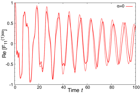
(b)

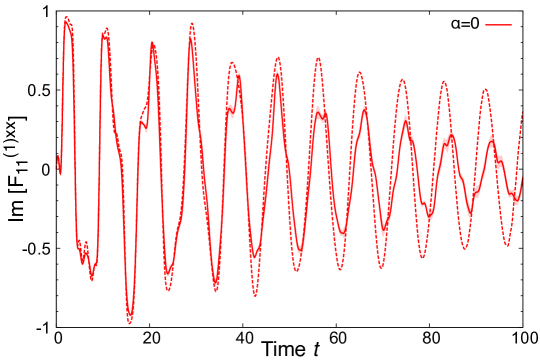
(c)

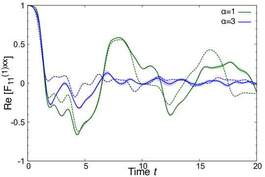
(d)

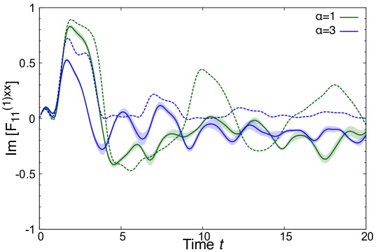
Figure 1: The real part and the imaginary part of autocorrelation functions. The DTWA results and exact results are drawn by bold lines and dotted lines, respectively. (a) and (b) show the data at $\alpha=0$ with $N=50$, whereas (c) and (d) show the data at $\alpha=1$ (green) and $\alpha=3$ (blue) with $N=15$. The shaded regions represent the standard deviation.

We consider the following quantities:

$$F_{ii}^{(1)aa}(t)= \langle\hat{\sigma}_{i}^{a}(t)\hat{\sigma}_{i}^{a}\rangle,$$

$$C_{ij}^{(n)ab}(t)= \frac{1}{2}\lVert[\hat{\sigma}_{i}^{a}(t),\hat{\sigma}_{j}^{b}]\rVert_{2n},$$ (15)

where $i,j\in\Lambda$, $a,b\in\{x,y,z\}$, $[\cdot,\cdot]$ denotes the commutator, and $\lVert\cdot\rVert_{2n}$ is the scaled Schatten $2n$-norms, defined by $\lVert\hat{O}\rVert_{2n}=(\langle(\hat{O}^{\dagger}\hat{O})^{n}\rangle)^{1/2n}$. The first quantity is the autocorrelation function, which plays a pivotal role in linear-response theory [26] and Krylov complexity [27]. The second quantity describes quantum information scrambling. The Frobenius norm corresponding to $n=1$ and the operator norm corresponding to $n\to\infty$ were studied in previous works [11, 14, 13]. The Frobenius and operator norms represent the average and the fastest spreading of quantum information, respectively, and yield different lower bounds on $\gamma$ [11, 13]. The monotonicity of the scaled Schatten norm, described by for any $\rho$

$$C_{ij}^{(n)ab}(t)\leq C_{ij}^{(n+1)ab}(t),$$ (16)

indicates that the scaled Schatten norm with larger $n$ gives a better bound for the operator norm.

The scaled Schatten norm is related to the OTOC as

$$C_{ij}^{(n)ab}(t)=\frac{1}{2}\left[\binom{2n}{n}\left(1+2\sum_{k=1}^{n}\frac{(-1)^{k}\binom{n}{k}}{\binom{n+k}{k}}F_{ij}^{(2k)ab}(t)\right)\right]^{\frac{1}{2n}}.$$ (17)

This relation is obtained by the binomial expansion of $(\hat{A}-\hat{B})^{2n}$, where $\hat{A}=\hat{\sigma}_{i}^{a}(t)\hat{\sigma}_{j}^{b}$ and $\hat{B}=\hat{\sigma}_{j}^{b}\hat{\sigma}_{i}^{a}(t)$, with properties of $\hat{A}\hat{B}=\hat{B}\hat{A}=\hat{I}$.

(a)

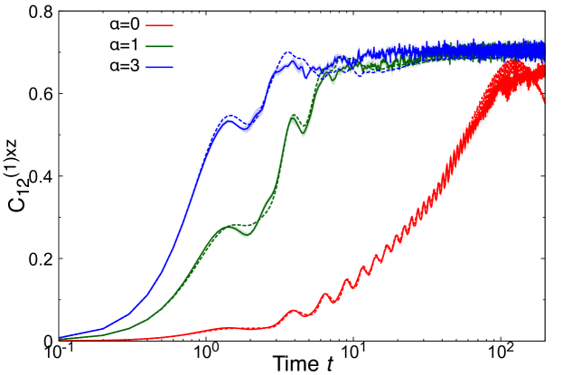
(b)

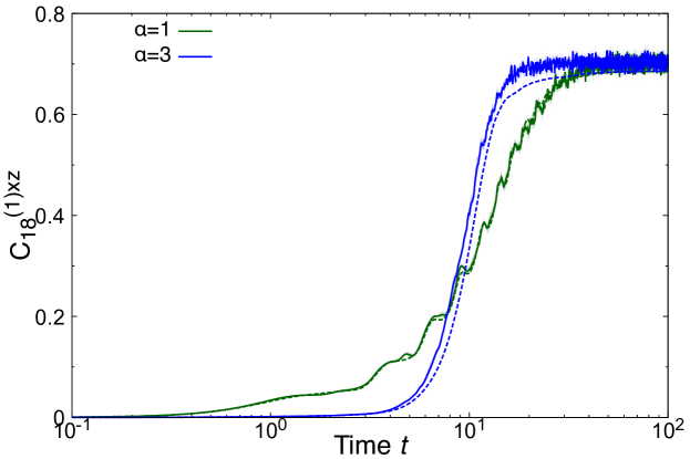
(c)

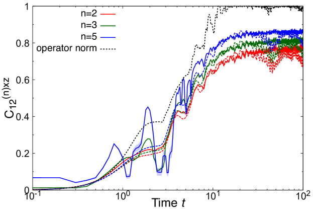
Figure 2: The OTOC results. The DTWA results and exact results are drawn by bold lines and dotted lines, respectively. (a) $C_{12}^{(1)xz}(t)$ and (b) $C_{1\lceil(N+1)/2\rceil}^{(1)xz}(t)$ with $\rho=\rho_{0}$ are depicted for various values of $\alpha$: $\alpha=0$ and $N=50$ (red), $\alpha=1$ and $N=15$ (green), and $\alpha=3$ and $N=15$ (blue). (c) $C_{12}^{(n)xz}(t)$ with $\rho=\rho_{0}$ at $n=2$ (red), $n=3$ (green), and $n=5$ (blue) at $\alpha=0$ and $N=10$ are depicted. The black dotted line represents the operator norm. The shaded regions represent the standard deviation.

Figure 1 depicts the real and imaginary parts of the autocorrelation function, $F_{11}^{(1)xx}(t)$, with the density matrix of $\rho=\rho_{\downarrow}$ for various values of $\alpha$ (see Appendix C for the system-size dependences of the results). We find that the DTWA accurately reproduces the multiple oscillations of the exact dynamics for both real and imaginary parts at $\alpha=0$. For all the cases, the DTWA captures the initial stage of the exact dynamics, but deviations from the exact dynamics appear earlier as $\alpha$ increases. It is noted that the mean-field (MF) approach can not accurately capture even the initial dynamics. In the case of $F_{11}^{(1)xx}(t)$ with $\rho=\rho_{\downarrow}$, the MF approximation yields

$$F_{11}^{(1)xx}(t)\approx s_{1}^{x}(t)s_{1}^{x}(0)=0,$$ (18)

where $\bm{s}_{k}(t)$ are the solutions of classical equations of motions in Eq. (6) with initial conditions $(s_{k}^{x}(0),s_{k}^{y}(0),s_{k}^{z}(0))=(0,0,-1)$ for $k\in\Lambda$. This result clearly shows that the DTWA method, which accounts for the quantum fluctuations in $\rho$, outperforms the MF approach.

Figures 2 (a) and (b) illustrate the time evolution of the squared commutators, $C_{12}^{(1)xz}(t)$ and $C_{1\lceil(N+1)/2\rceil}^{(1)xz}(t)$ with $\rho=\rho_{0}$, for various values of $\alpha$, where $\lceil\cdot\rceil$ is the ceiling function. We do not depict $C_{1\lceil(N+1)/2\rceil}^{(1)xz}(t)$ for $\alpha=0$, since $C_{12}^{(1)xz}(t)=C_{1\lceil(N+1)/2\rceil}^{(1)xz}(t)$ in this case. For all the cases, the squared commutators start at zero, increase with time, and saturate at late times. The DTWA quantitatively reproduces the exact dynamics of $C_{12}^{(1)xz}(t)$ regardless of the value of $\alpha$. While the DTWA accurately captures the dynamics of $C_{1\lceil(N+1)/2\rceil}^{(1)xz}(t)$ at $\alpha=1$, it shows a noticeable deviation at $\alpha=3$. These results indicate the validity of the DTWA method for estimating the average spreading of quantum information in the strongly long-range interacting systems (i.e., $0\leq\alpha\leq 1$).

Figure 2 (c) presents the time-evolution of $C_{12}^{(n)xz}(t)$ with $\rho=\rho_{0}$ for higher order $n\in\{2,3,5\}$ at $\alpha=0$. The DTWA captures the saturated value of $C_{12}^{(n)xz}(t)$ at late times, but fails to describe the transient dynamics. The deviations increase with the order $n$. We find that $C_{12}^{(5)xz}(t)$ exhibits large fluctuations , and thus does not even qualitatively align with the exact dynamics. The large fluctuations at $n=5$ remain for larger system size at $N=50$ (not shown). Capturing $C_{12}^{(n)xz}(t)$ for large $n$ is difficult, since the parenthesis in Eq. (17) at short-time scales is exponentially small with $n$. The standard deviation of $C_{12}^{(n)xz}(t)$ is small compared to its mean, indicating that these deviations arise from the intrinsic limitations of the DTWA method, rather than insufficient sampling. Furthermore, since $C_{12}^{(n)xz}(t)$ for a small $n$ significantly differs from $C_{12}^{(\infty)xz}(t)$, developing a method to estimate the fastest spreading of quantum information, represented by the operator norm $C_{ij}^{(\infty)ab}(t)$, remains a challenging open problem.

IV Conclusion

This paper proposes a DTWA-based method for computing the OTOC. The method is applied to analyze the time evolution of autocorrelation functions, squared commutators, and their higher-order extensions under Hamilton dynamics in long-range interacting systems. By comparing the DTWA method with exact computations, we demonstrate that the DTWA accurately captures the average spreading of quantum information (i.e., squared commutators) across all time regimes in the strongly long-range interacting systems (Figs. 2 (a) and (b)). However, we also identify the limitations of the DTWA method in studying weakly long-range interacting systems and the fastest spreading of quantum information. Although this benchmarking study limits the system size (e.g., $N=15$ at $\alpha=1$) for comparison with exact dynamics, the DTWA method is applicable to larger system sizes, even for $\alpha>0$. In future work, we aim to investigate the system-size dependence of scrambling time, described by $t_{*}\sim N^{\gamma}$, for large system sizes where exact numerical computations (i.e., numerical integration of the Schrödinger equation) are not accessible. Additionally, extending the DTWA method to finite temperature and disordered systems will be crucial.

Appendix A DTWA expression for OTOC

We give a DTWA expression for the $n$-th order OTOC $F_{ij}^{(n)ab}(t)$. In the discrete phase space, the $n$-th order OTOC is expressed as

$$F_{ij}^{(n)ab}(t)=\sum_{\bm{\tau}}W_{\bm{\tau}}\mathrm{Tr}[(\hat{\sigma}_{i}^{a}(t)\hat{\sigma}_{j}^{b})^{n}\hat{A}(\bm{s}_{\bm{\tau}})].$$ (19)

Let us introduce

$$G_{ij}^{(n)ab}(\bm{s}_{m}^{(0)}(\bm{\tau}))=\mathrm{Tr}[(\hat{\sigma}_{i}^{a}(t)\hat{\sigma}_{j}^{b})^{n-1}\hat{\sigma}_{i}^{a}(t)\hat{A}(\bm{s}_{m}^{(0)}(\bm{\tau}))].$$ (20)

Then the real part of the trace in $F_{ij}^{(n)ab}(t)$ is given as

$$\mathrm{Re}\mathrm{Tr}[(\hat{\sigma}_{i}^{a}(t)\hat{\sigma}_{j}^{b})^{n}\hat{A}(\bm{s}_{\bm{\tau}})]$$

$$= \frac{1}{2}\mathrm{Tr}[(\hat{\sigma}_{i}^{a}(t)\hat{\sigma}_{j}^{b})^{n-1}\hat{\sigma}_{i}^{a}(t)\{\hat{\sigma}_{j}^{b},\hat{A}(\bm{s}_{\bm{\tau}})\}]$$

$$= s_{\tau_{j}}^{b}\mathrm{Tr}[(\hat{\sigma}_{i}^{a}(t)\hat{\sigma}_{j}^{b})^{n-1}\hat{\sigma}_{i}^{a}(t)\hat{A}(\bm{s}_{1}^{(0)}(\bm{\tau}))]$$

$$= s_{\tau_{j}}^{b}G_{ij}^{(n)ab}(\bm{s}_{1}^{(0)}(\bm{\tau})),$$ (21)

where $\{\cdot,\cdot\}$ is the anticommutator, and the imaginary part of the trace in $F_{ij}^{(n)ab}(t)$ is expressed as

$$\mathrm{Im}\mathrm{Tr}[(\hat{\sigma}_{i}^{a}(t)\hat{\sigma}_{j}^{b})^{n}\hat{A}(\bm{s}_{\bm{\tau}})]$$

$$= \frac{-\mathrm{i}}{2}\mathrm{Tr}[(\hat{\sigma}_{i}^{a}(t)\hat{\sigma}_{j}^{b})^{n-1}\hat{\sigma}_{i}^{a}(t)[\hat{\sigma}_{j}^{b},\hat{A}(\bm{s}_{\bm{\tau}})]]$$

$$= \mathrm{Tr}[(\hat{\sigma}_{i}^{a}(t)\hat{\sigma}_{j}^{b})^{n-1}\hat{\sigma}_{i}^{a}(t)(\hat{A}(\bm{s}_{2}^{(0)}(\bm{\tau}))-\hat{A}(\bm{s}_{3}^{(0)}(\bm{\tau})))]$$

$$= G_{ij}^{(n)ab}(\bm{s}_{2}^{(0)}(\bm{\tau}))-G_{ij}^{(n)ab}(\bm{s}_{3}^{(0)}(\bm{\tau})).$$ (22)

For $n\geq 3$, we can show

$$G_{ij}^{(n)ab}(\bm{s}_{m}^{(0)}(\bm{\tau}))$$

$$= \mathrm{Tr}[\hat{\sigma}_{j}^{b}(\hat{\sigma}_{i}^{a}(t)\hat{\sigma}_{j}^{b})^{n-2}\hat{\sigma}_{i}^{a}(t)\hat{A}(\bm{s}_{m}^{(0)}(\bm{\tau}))\hat{\sigma}_{i}^{a}(t)]$$

$$\approx \mathrm{Tr}[\hat{\sigma}_{j}^{b}(\hat{\sigma}_{i}^{a}(t)\hat{\sigma}_{j}^{b})^{n-2}e^{\mathrm{i}\hat{H}t}\hat{\sigma}_{i}^{a}\hat{A}(\bm{s}_{m}^{(0)}(t;\bm{\tau}))\hat{\sigma}_{i}^{a}e^{-\mathrm{i}\hat{H}t}]$$

$$= \mathrm{Tr}[\hat{\sigma}_{j}^{b}(\hat{\sigma}_{i}^{a}(t)\hat{\sigma}_{j}^{b})^{n-2}e^{\mathrm{i}\hat{H}t}\hat{A}(\bm{s}_{m}^{(1)}(\bm{\tau}))e^{-\mathrm{i}\hat{H}t}]$$

$$\approx \mathrm{Tr}[(\hat{\sigma}_{i}^{a}(t)\hat{\sigma}_{j}^{b})^{n-3}\hat{\sigma}_{i}^{a}(t)\hat{\sigma}_{j}^{b}\hat{A}(\bm{s}_{m}^{(1)}(-t;\bm{\tau}))\hat{\sigma}_{j}^{b}]$$

$$= \mathrm{Tr}[(\hat{\sigma}_{i}^{a}(t)\hat{\sigma}_{j}^{b})^{n-3}\hat{\sigma}_{i}^{a}(t)\hat{A}(\bm{s}_{m}^{(2)}(\bm{\tau}))]$$

$$= G_{ij}^{(n-2)ab}(\bm{s}_{m}^{(2)}(\bm{\tau})).$$ (23)

By iteratively using this relation, we obtain for odd $n$

$$G_{ij}^{(n)ab}(\bm{s}_{m}^{(0)}(\bm{\tau}))= G_{ij}^{(1)ab}(\bm{s}_{m}^{(n-1)}(\bm{\tau}))$$

$$\approx \mathrm{Tr}[\hat{\sigma}_{i}^{a}\hat{A}(\bm{s}_{m}^{(n-1)}(t;\bm{\tau}))]$$

$$= s_{i,m}^{(n-1)a}(t;\bm{\tau})=s_{i,m}^{(n)a}(\bm{\tau}),$$ (24)

and for even $n$

$$G_{ij}^{(n)ab}(\bm{s}_{m}^{(0)}(\bm{\tau}))= G_{ij}^{(2)ab}(\bm{s}_{m}^{(n-2)}(\bm{\tau}))$$

$$\approx \mathrm{Tr}[\hat{\sigma}_{j}^{b}e^{\mathrm{i}\hat{H}t}\hat{\sigma}_{i}^{a}\hat{A}(\bm{s}_{m}^{(n-2)}(t;\bm{\tau}))\hat{\sigma}_{i}^{a}e^{-\mathrm{i}\hat{H}t}]$$

$$= \mathrm{Tr}[\hat{\sigma}_{j}^{b}e^{\mathrm{i}\hat{H}t}\hat{A}(\bm{s}_{m}^{(n-1)}(\bm{\tau}))e^{-\mathrm{i}\hat{H}t}]$$

$$\approx \mathrm{Tr}[\hat{\sigma}_{j}^{b}\hat{A}(\bm{s}_{m}^{(n-1)}(-t;\bm{\tau}))]$$

$$= s_{j,m}^{(n-1)b}(-t;\bm{\tau})=s_{j,m}^{(n)b}(\bm{\tau}).$$ (25)

Combining Eqs. (19), (21), (22), (24), and (25) obtains the DTWA expression for OTOCs in Eqs. (8) and (9).

Appendix B Exact simulation method at $\alpha=0$

Here we explain the exact simulation method of the autocorrelation function $F_{ii}^{(1)aa}(t)$ with $\rho=\rho_{\downarrow}$ and $\rho=\rho_{0}$, and the OTOC $F_{ij}^{(2)ab}(t)$ with $\rho=\rho_{0}$. The permutation symmetry of the Hamiltonian at $\alpha=0$ allows for the exact simulation even for large system sizes. The OTOC was computed in [16], but providing a detailed explanation here would be beneficial. Following the argument in [25], we introduce a basis element as

$$\ket{n_{11},\bm{u}_{11},n_{10},\bm{u}_{10}}\bra{n_{11},\bm{u}_{11},n_{01},\bm{u}_{01}},$$ (26)

where $n_{ij}$ represents the number of spins that are represented by $\ket{i}\bra{j}$, where $\ket{1}$ and $\ket{0}$ are eigenvectors of $\hat{\sigma}^{z}$ with the eigenvalue of $1$ and $-1$, respectively, and $\bm{u}_{ij}$ is the set of spin labels. For example, the basis denoted by $\ket{1,\{3\},0,\varnothing}\bra{1,\{3\},2,\{1,4\}}$ with $N=4$ represents a state, where spins $1$ and $4$ are in $\ket{0}\bra{1}$ state, spin $3$ is in $\ket{1}\bra{1}$ state, and spin $2$ is in $\ket{0}\bra{0}$ state. Here, $\varnothing$ denotes the empty set. Since $\bm{u}_{ij}$ is irrelevant within the subspace of the permutation symmetry, we define a basis $\hat{\Sigma}_{\vec{n}}$ as

$$C_{\vec{n}}\hat{\Sigma}_{\vec{n}}=\sum_{\text{all comb.}}\ket{n_{11},\bm{u}_{11},n_{10},\bm{u}_{10}}\bra{n_{11},\bm{u}_{11},n_{01},\bm{u}_{01}},$$ (27)

where the sum runs over all possible sets of $\bm{u}_{11}$, $\bm{u}_{10}$, and $\bm{u}_{01}$, and $\vec{n}=(n_{1},n_{2},n_{3})$ represents $n_{1}=n_{11}+n_{10}$, $n_{2}=n_{11}$, and $n_{3}=n_{01}$. The normalization is given by

$$C_{\vec{n}}=\frac{N!}{(n_{1}-n_{2})!n_{2}!n_{3}!(N-n_{1}-n_{3})!}.$$ (28)

Here, we adopt the notation, where $n_{1}$, $n_{2}$, and $n_{3}$ corresponds to $n$, $m$, and $m^{\prime}$ in Ref. [24], respectively. Then, the operators that belong to the permutation-symmetry subspace can be expressed as

$$\hat{A}=\sum_{n_{1}=0}^{N}\sum_{n_{2}=0}^{n_{1}}\sum_{n_{3}=0}^{N-n_{1}}A_{\vec{n}}\hat{\Sigma}_{\vec{n}},$$ (29)

where $A_{\vec{n}}\in\mathbb{C}$ is a coefficient. For example, the identity operator and all-spin-down state is expressed as $\hat{I}=\sum_{n_{1}=0}^{N}C_{(n_{1},0,0)}\hat{\Sigma}_{(n_{1},0,0)}$ and $\rho_{\downarrow}=\hat{\Sigma}_{(0,0,0)}$, respectively. Eq. (27) gives the inner product of $\hat{\Sigma}_{\vec{n}}$ and $\hat{\Sigma}_{\vec{n}^{\prime}}$ as

$$\mathrm{Tr}[\hat{\Sigma}_{\vec{n}}\hat{\Sigma}_{\vec{n}^{\prime}}]=\frac{1}{C_{\vec{n}}}\delta_{n^{\prime}_{1},n_{2}+n_{3}}\delta_{n^{\prime}_{2},n_{2}}\delta_{n^{\prime}_{3},n_{1}-n_{2}}.$$ (30)

To consider the time evolution of a spin operator $\hat{\bm{\sigma}}_{i}(t)=e^{\mathrm{i}\hat{H}t}\hat{\bm{\sigma}}_{i}e^{-\mathrm{i}\hat{H}t}$, we introduce a basis, where $\hat{\Sigma}_{\vec{n}}$ is sandwiched by spin operators, and expand $\hat{\bm{\sigma}}_{i}(t)$ using this basis as

$$\hat{\bm{\sigma}}_{i}(t)=\sum_{p,q\in\{1,x,y,z\}}\sum_{\vec{n}}{\bm{\sigma}}^{(p,q)}_{\vec{n}}(t)\hat{\sigma}_{i}^{p}\hat{\Sigma}_{\vec{n}}\hat{\sigma}_{i}^{q},$$ (31)

where $\hat{\sigma}_{i}^{1}$ is the identity operator and ${\bm{\sigma}}^{(p,q)}_{\vec{n}}(t)\in\mathbb{C}$ is a coefficient. The Heisenberg equation $d\hat{\bm{\sigma}}_{i}(t)/dt=\mathrm{i}[\hat{H},\hat{\bm{\sigma}}_{i}(t)]$ gives a set of differential equations for each element ${\bm{\sigma}}^{p,q}_{\vec{n}}(t)$. The number of equations is the order of $N^{3}$.

There is a relation between the basis $\hat{\Sigma}_{\vec{n}}$ and $\sum_{i\in\Lambda}\hat{\sigma}_{i}^{p}\hat{\Sigma}_{\vec{n}}\hat{\sigma}_{i}^{q}$:

$$\sum_{i\in\Lambda}\hat{\sigma}_{i}^{p}\hat{\Sigma}_{\vec{n}}\hat{\sigma}_{i}^{q}=\sum_{\vec{n}^{\prime}}f_{\vec{n},\vec{n}^{\prime}}^{p,q}\hat{\Sigma}_{\vec{n}^{\prime}},$$ (32)

where $f_{\vec{n},\vec{n}^{\prime}}^{p,q}\in\mathbb{C}$ is a coefficient. For example, $f_{\vec{n},\vec{n}^{\prime}}^{z,z}=[N-2(n_{1}-n_{2}+n_{3})]\delta_{\vec{n},\vec{n}^{\prime}}$. Then, we can compute the following quantity using Eq. (30) and Eq. (32):

$$g_{\vec{n},\vec{n}^{\prime}}^{\vec{p},\vec{q}}=\sum_{i\in\Lambda}\mathrm{Tr}[(\hat{\sigma}_{i}^{p_{1}}\ldots\hat{\sigma}_{i}^{p_{m}})\hat{\Sigma}_{\vec{n}}(\hat{\sigma}_{i}^{q_{1}}\ldots\hat{\sigma}_{i}^{q_{m}})\hat{\Sigma}_{\vec{n}^{\prime}}].$$ (33)

Here, $\vec{p}=(p_{1},\ldots,p_{m})$ and $\vec{q}=(q_{1},\ldots,q_{m})$, where $m$ represents the length of the vectors, and $p_{i},q_{i}\in\{1,x,y,z\}$.

First we consider an antocorrelation function: $F_{ii}^{(1)aa}(t)=\mathrm{Tr}[\hat{\sigma}_{i}^{a}(t)\hat{\sigma}_{i}^{a}\rho]$. For $\rho=\rho_{\downarrow}$,

$$F_{ii}^{(1)aa}(t)=\frac{1}{N}\sum_{k\in\Lambda}F_{kk}^{(1)aa}(t)$$

$$= \frac{1}{N}\sum_{k\in\Lambda}\mathrm{Tr}[\hat{\sigma}_{k}^{a}(t)\hat{\sigma}_{k}^{a}\rho_{\downarrow}]$$

$$= \frac{1}{N}\sum_{p,q}\sum_{\vec{n}}\sum_{k\in\Lambda}{\sigma}^{a(p,q)}_{\vec{n}}(t)\mathrm{Tr}[(\hat{\sigma}_{k}^{p}\hat{\Sigma}_{\vec{n}}\hat{\sigma}_{k}^{q})(\hat{\sigma}_{k}^{a}\hat{\Sigma}_{\vec{0}})]$$

$$= \frac{1}{N}\sum_{p,q}\sum_{\vec{n}}{\sigma}^{a(p,q)}_{\vec{n}}(t)g_{\vec{n},\vec{0}}^{(p,1),(q,a)}.$$ (34)

In the first line, we use translational symmetry. From the second to the third line, we apply Eq. (31) and $\rho_{\downarrow}=\hat{\Sigma}_{\vec{0}}$. In the last line, we use the expression in Eq. (33). Similarly, we obtain $F_{ii}^{(1)aa}(t)$ with $\rho=\rho_{0}$ by noting that $\rho_{0}=2^{-N}\sum_{n_{1}=0}^{N}C_{(n_{1},0,0)}\hat{\Sigma}_{(n_{1},0,0)}$.

Next we consider an OTOC at infinite temperature state: $F_{ij}^{(2)ab}(t)=\mathrm{Tr}[\hat{\sigma}_{i}^{a}(t)\hat{\sigma}_{j}^{b}\hat{\sigma}_{i}^{a}(t)\hat{\sigma}_{j}^{b}]/2^{N}$ for $i\neq j$. The permutation symmetry implies that

$$F_{ij}^{(2)ab}(t)=\frac{1}{N(N-1)}\left[\sum_{k,\ell\in\Lambda}F_{k\ell}^{(2)ab}(t)-\sum_{k\in\Lambda}F_{kk}^{(2)ab}(t)\right].$$ (35)

The first term is given as

$$\sum_{k,\ell\in\Lambda}F_{k\ell}^{(2)ab}(t)= \frac{1}{2^{N}}\sum_{k,\ell\in\Lambda}\mathrm{Tr}[\hat{\sigma}_{k}^{a}(t)\hat{\sigma}_{\ell}^{b}\hat{\sigma}_{k}^{a}(t)\hat{\sigma}_{\ell}^{b}].$$ (36)

Substituting into Eq. (36) the following relation

$$\sum_{\ell\in\Lambda}\hat{\sigma}_{\ell}^{b}\hat{\sigma}_{k}^{a}(t)\hat{\sigma}_{\ell}^{b}=\sum_{\ell\in\Lambda}\sum_{p,q}\sum_{\vec{n}}\sigma_{\vec{n}}^{(p,q)}(t)\hat{\sigma}_{\ell}^{b}\hat{\sigma}_{k}^{p}\hat{\Sigma}_{\vec{n}}\hat{\sigma}_{k}^{q}\hat{\sigma}_{\ell}^{b}$$

$$= \sum_{p,q}\sum_{\vec{n}}\Big{[}\sum_{\vec{n}^{\prime}}\sigma_{\vec{n}}^{a(p,q)}(t)f_{\vec{n},\vec{n}^{\prime}}^{b,b}\hat{\sigma}_{k}^{p}\hat{\Sigma}_{\vec{n}^{\prime}}\hat{\sigma}_{k}^{q}$$

$$-2\mathrm{i}\epsilon_{bpq}(\sigma_{\vec{n}}^{a(q,b)}(t)\hat{\sigma}_{k}^{p}\hat{\Sigma}_{\vec{n}}+\sigma_{\vec{n}}^{a(b,p)}(t)\hat{\Sigma}_{\vec{n}}\hat{\sigma}_{k}^{q})\Big{]}$$

$$= \sum_{p,q}\sum_{\vec{n}}h_{\vec{n}}^{ab(p,q)}(t)\hat{\sigma}_{k}^{p}\hat{\Sigma}_{\vec{n}}\hat{\sigma}_{k}^{q},$$ (37)

where $h_{\vec{n}}^{ab(p,q)}(t)\in\mathbb{C}$ is a coefficient and $\epsilon_{bpq}$ is the Levi-Civita symbol, yields

$$\sum_{k,\ell\in\Lambda}F_{k\ell}^{(2)ab}(t)= \frac{1}{2^{N}}\sum_{p,q,r,s}\sum_{\vec{n},\vec{n}^{\prime}}h_{\vec{n}}^{ab(p,q)}(t)g_{\vec{n},\vec{n}^{\prime}}^{(s,p),(q,r)}\sigma_{\vec{n}^{\prime}}^{(r,s)}(t).$$ (38)

Similarly, we obtain

$$\sum_{k\in\Lambda}F_{kk}^{(2)ab}(t)=\frac{1}{2^{N}}\sum_{k\in\Lambda}\mathrm{Tr}[\hat{\sigma}_{k}^{a}(t)\hat{\sigma}_{k}^{b}\hat{\sigma}_{k}^{a}(t)\hat{\sigma}_{k}^{b}]$$

$$= \frac{1}{2^{N}}\sum_{p,q,r,s}\sum_{\vec{n},\vec{n}^{\prime}}\sigma_{\vec{n}}^{a(p,q)}(t)\sigma_{\vec{n}^{\prime}}^{a(r,s)}(t)g_{\vec{n},\vec{n}^{\prime}}^{(s,b,p),(q,b,r)}.$$ (39)

Thus, Substituting Eqs. (38) and (39) into Eq. (35) provides the OTOC $F_{ij}^{(2)ab}(t)$ with $\rho=\rho_{0}$.

Appendix C System-size dependences of DTWA method

Autocorrelation function $F_{11}^{(1)xx}(t)$ with $\rho=\rho_{\downarrow}$

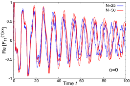
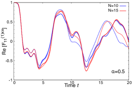
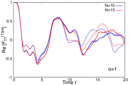
Autocorrelation function $F_{11}^{(1)xx}(t)$ with $\rho=\rho_{0}$

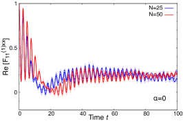
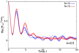
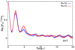
Frobenius norm $C_{12}^{(1)xz}(t)$

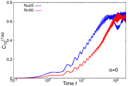
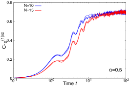
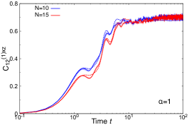
Figure 3: $F_{11}^{(1)xx}(t)$ with $\rho=\rho_{\downarrow}$ (upper panels), $F_{11}^{(1)xx}(t)$ with $\rho=\rho_{0}$ (middle panels), and $C_{12}^{(1)xz}(t)$ (lower panels) at various values of $\alpha\in\{0,0.5,1\}$. The red and blue lines represent the results for the larger and the smaller system sizes, respectively. The bold lines indicate the DTWA results, whereas the dotted lines correspond to the exact results. The shaded regions depict the standard deviation of the DTWA results.

We present system-size dependences of the DTWA method in strongly long-range interacting systems at $\alpha\in\{0,0.5,1\}$. The DTWA captures longer-time dynamics of $F_{11}^{(1)xx}(t)$ at $\alpha\in\{0,0.5\}$ with $\rho=\rho_{\downarrow}$ and $\rho_{0}$ as the system size increases. On the other hand, at $\alpha=1$, where the interaction lies at the boundary, the DTWA reproduces the exact dynamics for almost the same duration across different system sizes. For $C_{12}^{(1)xz}(t)$, the DTWA reproduces the exact dynamics even for small system sizes at all values of $\alpha$. Additionally, at $\alpha=0$, we observe oscillations in $C_{12}^{(1)xz}(t)$ at late times, which are not captured by the DTWA method.

References

• Larkin and Ovchinnikov [1969] A. I. Larkin and Y. N. Ovchinnikov, Journal of Experimental and Theoretical Physics  (1969), Quasiclassical Method in the Theory of Superconductivity.
• Swingle [2018] B. Swingle, Nature Physics 14, 988 (2018), Unscrambling the physics of out-of-time-order correlators.
• Maldacena et al. [2016] J. Maldacena, S. H. Shenker, and D. Stanford, Journal of High Energy Physics 2016, 106 (2016), A bound on chaos.
• Bentsen et al. [2019] G. Bentsen, Y. Gu, and A. Lucas, Proceedings of the National Academy of Sciences 116, 6689 (2019), Fast scrambling on sparse graphs.
• Shenker and Stanford [2014] S. H. Shenker and D. Stanford, Journal of High Energy Physics 2014, 67 (2014), Black holes and the butterfly effect.
• Lieb and Robinson [1972] E. H. Lieb and D. W. Robinson, Communications in Mathematical Physics 28, 251 (1972), The finite group velocity of quantum spin systems.
• Gärttner et al. [2017] M. Gärttner, J. G. Bohnet, A. Safavi-Naini, M. L. Wall, J. J. Bollinger, and A. M. Rey, Nature Physics 13, 781 (2017), Measuring out-of-time-order correlations and multiple quantum spectra in a trapped-ion quantum magnet.
• Li et al. [2017] J. Li, R. Fan, H. Wang, B. Ye, B. Zeng, H. Zhai, X. Peng, and J. Du, Phys. Rev. X 7, 031011 (2017), Measuring Out-of-Time-Order Correlators on a Nuclear Magnetic Resonance Quantum Simulator.
• Braumüller et al. [2022] J. Braumüller, A. H. Karamlou, Y. Yanay, B. Kannan, D. Kim, M. Kjaergaard, A. Melville, B. M. Niedzielski, Y. Sung, A. Vepsäläinen, R. Winik, J. L. Yoder, T. P. Orlando, S. Gustavsson, C. Tahan, and W. D. Oliver, Nature Physics 18, 172 (2022), Probing quantum information propagation with out-of-time-ordered correlators.
• Defenu et al. [2023] N. Defenu, T. Donner, T. Macrì, G. Pagano, S. Ruffo, and A. Trombettoni, Rev. Mod. Phys. 95, 035002 (2023), Long-range interacting quantum systems.
• Tran et al. [2020] M. C. Tran, C.-F. Chen, A. Ehrenberg, A. Y. Guo, A. Deshpande, Y. Hong, Z.-X. Gong, A. V. Gorshkov, and A. Lucas, Phys. Rev. X 10, 031009 (2020), Hierarchy of Linear Light Cones with Long-Range Interactions.
• Yin and Lucas [2020] C. Yin and A. Lucas, Phys. Rev. A 102, 022402 (2020), Bound on quantum scrambling with all-to-all interactions.
• Kuwahara and Saito [2021] T. Kuwahara and K. Saito, Phys. Rev. Lett. 126, 030604 (2021), Absence of Fast Scrambling in Thermodynamically Stable Long-Range Interacting Systems.
• Colmenarez and Luitz [2020] L. Colmenarez and D. J. Luitz, Phys. Rev. Res. 2, 043047 (2020), Lieb-Robinson bounds and out-of-time order correlators in a long-range spin chain.
• Richter et al. [2023] J. Richter, O. Lunt, and A. Pal, Phys. Rev. Res. 5, L012031 (2023), Transport and entanglement growth in long-range random Clifford circuits.
• Qi et al. [2023] Z. Qi, T. Scaffidi, and X. Cao, Phys. Rev. B 108, 054301 (2023), Surprises in the deep Hilbert space of all-to-all systems: From superexponential scrambling to slow entanglement growth.
• Schachenmayer et al. [2015] J. Schachenmayer, A. Pikovski, and A. M. Rey, Phys. Rev. X 5, 011022 (2015), Many-Body Quantum Spin Dynamics with Monte Carlo Trajectories on a Discrete Phase Space.
• Wootters [1987] W. K. Wootters, Annals of Physics 176, 1 (1987), A Wigner-function formulation of finite-state quantum mechanics.
• Mori [2019] T. Mori, Journal of Physics A: Mathematical and Theoretical 52, 054001 (2019), Prethermalization in the transverse-field Ising chain with long-range interactions.
• Kunimi et al. [2021] M. Kunimi, K. Nagao, S. Goto, and I. Danshita, Phys. Rev. Res. 3, 013060 (2021), Performance evaluation of the discrete truncated Wigner approximation for quench dynamics of quantum spin systems with long-range interactions.
• Kac et al. [1963] M. Kac, G. E. Uhlenbeck, and P. C. Hemmer, Journal of Mathematical Physics 4, 216 (1963), On the van der Waals Theory of the Vapor‐Liquid Equilibrium. I. Discussion of a One‐Dimensional Model.
• Kim et al. [2014] H. Kim, T. N. Ikeda, and D. A. Huse, Phys. Rev. E 90, 052105 (2014), Testing whether all eigenstates obey the eigenstate thermalization hypothesis.
• Tsuji et al. [2018] N. Tsuji, T. Shitara, and M. Ueda, Phys. Rev. E 97, 012101 (2018), Out-of-time-order fluctuation-dissipation theorem.
• Sarkar and Satchell [1987] S. Sarkar and J. S. Satchell, Europhysics Letters 3, 797 (1987), Optical Bistability with Small Numbers of Atoms.
• Gegg and Richter [2016] M. Gegg and M. Richter, New Journal of Physics 18, 043037 (2016), Efficient and exact numerical approach for many multi-level systems in open system CQED.
• Kubo et al. [2012] R. Kubo, M. Toda, and N. Hashitsume, Statistical physics II: nonequilibrium statistical mechanics, Vol. 31 (Springer Science & Business Media, 2012).
• Parker et al. [2019] D. E. Parker, X. Cao, A. Avdoshkin, T. Scaffidi, and E. Altman, Phys. Rev. X 9, 041017 (2019), A Universal Operator Growth Hypothesis.
• Note [1] When the parenthesis in Eq. (17) is negative in numerical simulations, the value of $C_{12}^{(5)ab}(t)$ is set to zero.