The critical velocity of the bullet process appears pathwise

Abstract.

In the bullet process, a gun fires bullets in the same direction at independent random speeds. When two bullets collide, they vanish. The critical velocity is the slowest speed the first bullet can take and still have positive probability of surviving forever. We prove that the critical velocity is the $\limsup$ of the speeds of the bullets that survive from the last position in each truncation. This result allows us to prove several properties about the bullet process. Infinitely many bullets survive when the velocity distribution has finite support, and in general there is a zero-one law. We obtain continuity results for the probability of survival with respect to velocity. Along the way we answer a question from [BM20], showing that if a bullet survives, it does so in all but finitely many truncations of the bullet process.

1. Introduction

In the bullet process, bullets are fired from the origin and travel along $[0,\infty)$. Whenever a faster bullet catches up to a slower one, they both annihilate and are removed from the system. Bullet velocities are i.i.d., as are delays between firings. David Wilson first defined the bullet process in the canonical setting with unit delays and velocity distribution $\operatorname{Unif}(0,1)$ [KW14]. Figure 1 depicts a simulation of the process.

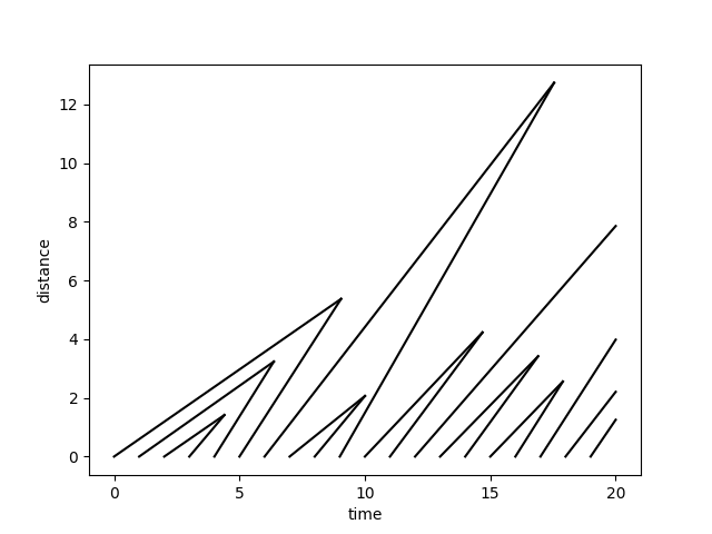
Figure 1. The time-space diagram for a sample path of the bullet process up to time $20$ in the setting with $\mu\sim\operatorname{Unif}(.5,1.5)$ and $\nu=1$. Time moves left to right, with bullets’ paths depicted vertically. (The velocity distribution is shifted up for visual clarity, to avoid near-hoizontal bullet paths.)

The bullet problem asks whether the first bullet survives with positive probability. In other words, let the critical velocity $v_{c}$, defined formally in Section 1.1, be the slowest velocity the first bullet can have and still survive with positive probability. $v_{c}\in[0,1]$ since a velocity $1$ bullet at the front almost surely survives while a velocity $0$ bullet is immediately annihilated by the second bullet at $t=1$. The bullet problem asks if $v_{c}<1$. Despite its simple setup, a solution has remained elusive over the last decade, lending its popularity. It is conjectured that $v_{c}\in(0,1)$, with our simulations placing it somewhere around $.75$ (see Figure 2). This would correct the word-of-mouth conjecture that $v_{c}\sim 0.9$ from [DKJ⁺19].

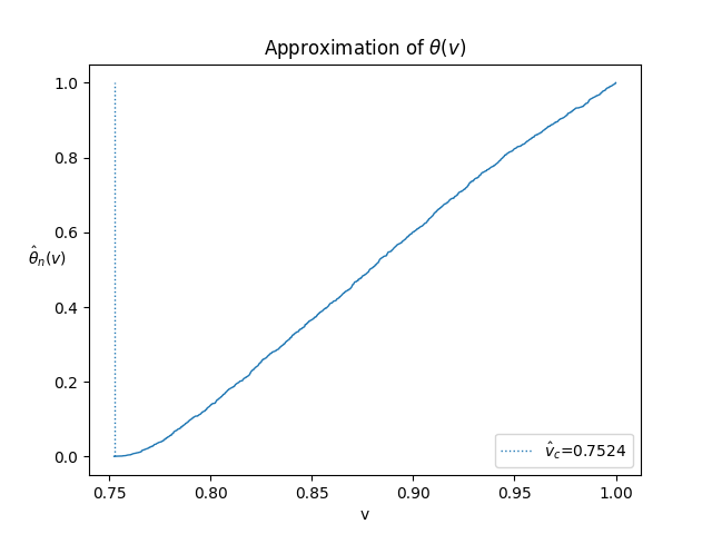
Figure 2. Let $\theta_{n}(v)$ be the probability the first bullet survives with velocity $v$ among $n$ bullets. Above, we choose $n=1$ billion, and graph $\hat{\theta}_{n}(v)$, the empirical estimation of $\theta_{n}(v)$ based on $N=2000$ simulations. By Theorem 6, $\theta_{n}(v)\to\theta(v)$ as $n\to\infty$. $\hat{v}_{c}\sim.7524$ is the minimal $v$ with $\hat{\theta}_{n}(v)>0$. $\hat{v}_{c}\overset{p}{\to}v_{c}$ letting $N\to\infty$ first and then $n\to\infty$.

We consider any non-negative velocity distribution $\mu$ and positive delay distribution $\nu$. Our main result states that $v_{c}$ arises as a deterministic function of the process, though defined as a property of the sample space. Formally defined in Section 1.1, we call the $n^{\text{th}}$ bullet, $\bullet_{n}$, a potential survivor if it survives when only bullets $(\bullet_{1},\ldots,\bullet_{n})$ are fired. Note that $\bullet_{n}$ survives if and only if it is a potential survivor, and also survives among $(\bullet_{n},\bullet_{n+1},\ldots)$. Both events are independent conditional on $\bullet_{n}$’s velocity. In every sample path, $v_{c}$ is equal to $\hat{v}$, the $\limsup$ of the velocities of potential survivors.

Throughout, all claims involving random variables hold almost surely.

Theorem 1.

$\hat{v}=v_{c}$ for any $\mu,\nu$.

By Theorem 1, we can numerically simulate the critical velocity from a single sample of the bullet process, as in Figure 3. Moreover, the result gives us a handle on the bullet process which we leverage to analyze other properties. For instance, a question we sought to answer was whether infinitely many bullets survive. We prove this is the case when there are finitely many velocities. See Figure 4 for a demonstration of this fact in a discretization of the bullet problem.

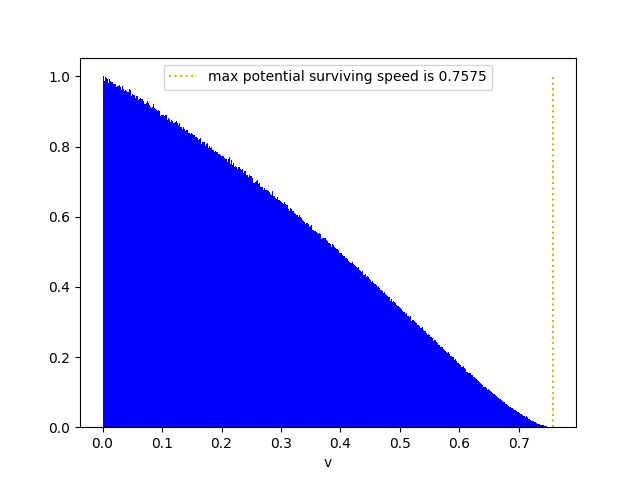
Figure 3. Approximation of $\hat{v}$ for two different simulations with $10^{8}$ bullets in the original setting of the bullet process. Histograms of the velocities of potential survivors from the second half of the process are shown. We use buckets of width .001 and normalize the y-axis so $1.0$ represents the expected number of bullets in that speed bucket, potential survivor or not. The yellow line displays the maximum speed of the potential survivors.

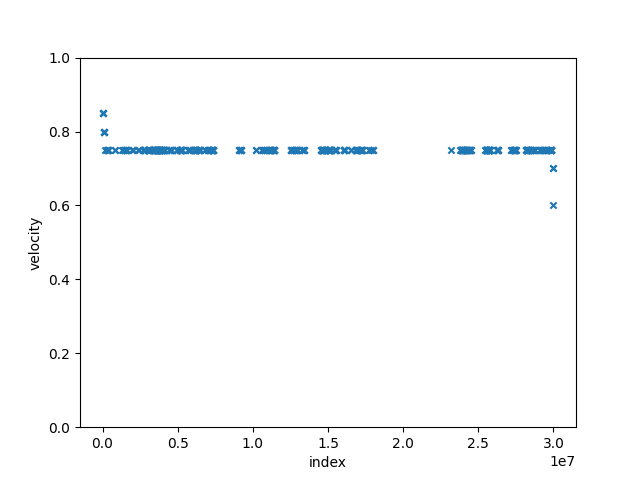
Figure 4. Two samples of $S_{n}$ for different uniform distributions on finite velocity sets. On the left, we use velocities $V_{1},\ldots,V_{100}$ where $V_{i}=i/100+\varepsilon_{i}$ and $\varepsilon_{i}\sim\mathcal{N}(0,.0002)$ is independent Gaussian noise added to avoid triple collisions. On the right we use the $20$ speeds $V_{5},V_{10},\ldots,V_{95},V_{100}$, that is $.05,.1,\ldots,.95,1.0$ plus noise. For the right, $n=30$ million and there are $574$ survivors. All but $12$ have velocity $V_{75}\sim.75$, with $9$ faster and $3$ slower at the end. On the left, we choose $n=1$ billion, as survivors are more spread out ([BM20] showed for non-atomic velocity distributions, $|S_{n}|$ grows logarithmically). There are $62$ survivors: $52$ have velocity $V_{76}\sim\!\!.76$, $6$ are faster, and $4$ slower. The first speed-$V_{76}$ survivor has index $\sim 48$ million.

Theorem 2.

When $\mu$ has finite support, infinitely many bullets survive. All but finitely many survivors have velocity $v_{c}$.

In [DKJ⁺19] it was shown that for $\mu$ uniform on a finite set of at least $3$ positive velocities, $v_{c}$ is neither the fastest nor the slowest velocity. For general velocity distributions, the best we were able to demonstrate was a zero-one law in Corollary 14.

We also use Theorem 1 to get continuity results for $\theta(v)$, the probability $\bullet_{1}$ survives when it has velocity $v$.

Theorem 3.

1. $\theta(v)$ is right-continuous everywhere.

2. For any $v>v_{c}$, $\theta(v)$ is discontinuous at $v$ if and only if $v$ is an atom of $\mu$.

3. Let $E$ denote the event that there are infinitely many potential survivors faster than $v_{c}$. The following are equivalent:

   1. $\theta(v)$ is continuous at $v_{c}$.

   2. $\theta(v)=0$.

   3. $\mathbf{P}(E)>0$.

   4. $\mathbf{P}(E)=1$.

Finally, we note that all of our results apply to one-sided ballistic annihilation. Ballistic annihilation is a closely related process studied by physicists to model the kinetics of chemical reactions [EF85]. All particles are present at time $0$ and have i.i.d. spacings. As noted in [ST17], by inverting the axes on the time-space diagram, one-sided ballistic annihilation is equivalent to the bullet process with inverted velocities. Using the linear speed-change invariance property from Section 2 of [ST17], all of our results apply to one-sided ballistic annihilation with velocity distribution bounded above or below.

1.1. Definitions and Notation

The bullet process $B=(B_{t})_{t\geq 0}$ is defined for a sequence of bullets $\vec{\bullet}\mkern 2.0mu\vphantom{\bullet}=(\bullet_{i})_{i\in\mathcal{J}}$, indexed by the finite or countable set $\mathcal{J}=\{i_{1},i_{2},\ldots\}\subset\mathbb{R}$ with $i_{1}<i_{2}<\ldots$ Typically $\mathcal{J}$ is a consecutive sequence of natural numbers, but we maintain the flexibility to add or remove bullets. Each $i\in\mathcal{J}$ indexes a bullet

$$\bullet_{i}=(i,v_{i},\delta_{i}),$$

where $v_{i}\geq 0$ is its velocity and $\delta_{i}>0$ specifies how long after the previous bullet it is fired, if there is one. That is, let $t_{n}$ be the time $\bullet_{n}$ is fired, with $t_{i_{1}}=0$. Then $t_{i_{n+1}}=t_{i_{n}}+\delta_{i_{n+1}}$ and $\delta_{i_{1}}$ is ignored. $(v_{i},\delta_{i})$ is drawn i.i.d. from $\Omega=\mu\times\nu$. The bullet problem refers to the context where $\mu\sim\operatorname{Unif}(0,1)$, $\nu=1$ deterministically, and $\mathcal{J}=\mathbb{N}_{>0}$.

$B=B(\vec{\bullet}\mkern 2.0mu\vphantom{\bullet})$ tracks which bullets are active and what their positions are. We define $B_{t}$ as the pair of functions $(a_{t},d_{t})$, with $a_{t}(i)\in\{0,1\}$ tracking if $\bullet_{i}$ is active, that is $t\geq t_{i}$ and $\bullet_{i}$ has not been annihilated yet, and $d_{t}(i)=v_{i}(t-t_{i})$ the position of $\bullet_{i}$ if it is active. We require $\mu,\nu$ to be such that a.s. no three active bullets can simultaneously collide, which is achieved if either $\mu$ or $\nu$ is continuous. For $j>i$, $\bullet_{j}\rightarrow\bullet_{i}$ denotes the annihilation event where $\bullet_{j}$ catches up to $\bullet_{i}$.

Throughout, $\vec{\bullet}\mkern 2.0mu\vphantom{\bullet}$ represents the countable sequence $(\bullet_{1},\bullet_{2},\ldots)$ with subsequences obtained via the following indexing conventions:

$$\vec{\bullet}\mkern 2.0mu\vphantom{\bullet}_{n} =(\bullet_{1},\ldots,\bullet_{n})$$

$$\vec{\bullet}\mkern 2.0mu\vphantom{\bullet}_{[m,n]} =(\bullet_{m},\ldots,\bullet_{n})$$

$$\vec{\bullet}\mkern 2.0mu\vphantom{\bullet}_{[n,\infty)} =(\bullet_{n},\bullet_{n+1},\ldots)$$

$\vec{\bullet}\mkern 2.0mu\vphantom{\bullet}_{n}=\vec{\bullet}\mkern 2.0mu\vphantom{\bullet}_{[1,n]}$ is redundant notation, but we use it as this is the most common case, pertaining to truncations. For index $I$ of the form $[m,n]$, $[n,\infty)$ or $n$, we denote the bullet process on $\vec{\bullet}\mkern 2.0mu\vphantom{\bullet}_{I}$ by $B_{I}:=B(\vec{\bullet}\mkern 2.0mu\vphantom{\bullet}_{I})$. To specify which bullet process a collision takes place in, we use phrases like $\bullet_{j}\rightarrow\bullet_{i}$ in $B_{n}$ or in $B_{[n,\infty)}$. By itself $\bullet_{j}\rightarrow\bullet_{i}$ generally means it occurs in $B=B(\vec{\bullet}\mkern 2.0mu\vphantom{\bullet})$.

We say $\bullet_{i}$ perishes if $\bullet_{j}\to\bullet_{i}$ or $\bullet_{i}\to\bullet_{j}$ for some $j$, otherwise we say it survives. $\bullet_{j}$ threatens $\bullet_{i}$ if $\bullet_{j}\rightarrow\bullet_{i}$ in $B_{j}$, which is a precondition for $\bullet_{j}$ annihilating $\bullet_{i}$ in $B(\vec{\bullet}\mkern 2.0mu\vphantom{\bullet})$. The set of surviving bullets in $B(\vec{\bullet}\mkern 2.0mu\vphantom{\bullet})$ is denoted

$$S=S(\vec{\bullet}\mkern 2.0mu\vphantom{\bullet}):=\{\bullet_{i}:\bullet_{i}\text{ survives in }B(\vec{\bullet}\mkern 2.0mu\vphantom{\bullet})\}.$$

$S_{I}=S(\vec{\bullet}\mkern 2.0mu\vphantom{\bullet}_{I})$ is the set of survivors for $B_{I}$. Of critical interest in this paper are the potential survivors, bullets which have a chance of survival at the time they are fired. We call $\bullet_{n}$ a potential survivor if it survives in $B_{n}=B(\bullet_{1},\ldots,\bullet_{n})$, i.e. $\bullet_{n}\in S_{n}$. $PS=PS(\vec{\bullet}\mkern 2.0mu\vphantom{\bullet})$ is the set of all such $\bullet_{n}$. Similarly, we define $PS_{I}:=PS(\vec{\bullet}\mkern 2.0mu\vphantom{\bullet}_{I})$, where for instance $PS_{[n,\infty)}$ is the set of all $\bullet_{n^{\prime}}$ that survive in $B_{[n,n^{\prime}]}$. Almost surely $|PS|=\infty$ since $\bullet_{n}\in PS$ whenever it is the slowest bullet among $\vec{\bullet}\mkern 2.0mu\vphantom{\bullet}_{[1,n]}$. So $PS=\{\bullet_{j_{1}},\bullet_{j_{2}},\ldots\}$ for the infinite increasing sequence $\{j_{n}\}$, and we can define

$$\hat{v}:=\limsup_{n\to\infty}\,\{v_{j_{n}}\}.$$

$\bullet_{n}$ survives behind if it survives in $B_{[n,\infty)}$. Note that $\bullet_{n}\in S$ if and only if it is a potential survivor and survives behind, so $S\subseteq PS$.

For any set of bullets $A$, let $A_{>v}$ denote $\{\bullet_{i}\in A:v_{i}>v\}$, and similarly define $A_{\geq v},A_{=v}$. So for instance $(S_{[n,\infty)})_{>v}$ is the set of survivors of $B_{[n,\infty)}$ with velocity greater than $v$.

$\theta(v)$ denotes the probability that $\bullet_{1}\in S$ given $v_{1}=v$. We define $\theta(v)$ for all $v\geq 0$, not just $v\in\operatorname{supp}\mu$, as follows. For $\bullet_{i}=(i,v_{i},\delta_{i})$ we change its velocity to $v$ by letting $\bullet^{v}_{i}=(i,v,\delta_{i})$. Then

$$\theta(v):=\mathbf{P}\left(\bullet_{1}^{v}\text{ survives in }B\left(\bullet_{1}^{v},\vec{\bullet}\mkern 2.0mu\vphantom{\bullet}_{[2,\infty)}\right)\right).$$

If $\theta(v)>0$, we say $v$ or a speed-$v$ bullet is fast or can survive, and otherwise is slow or can’t survive. The critical velocity is

$$v_{c}:=\inf\{v\geq 0:\theta(v)>0\}.$$

As discussed in the introduction, necessarily $v_{c}\in[0,\sup\mu]$. It does not follow immediately by definition that $v_{c}\in\operatorname{supp}\mu$, or even that $v_{c}\geq\inf\mu$, but this is indeed the case by Theorem 1.

1.2. Application to the Bullet Problem

Considering potential survivors opens up an avenue of attack for the bullet problem. For convenience, let the first bullet $\bullet_{0}^{v}$ have index $0$. $\bullet_{n}$ threatens $\bullet^{v}_{0}$ if and only if (i) $\bullet_{n}\in PS_{>v}=PS(\bullet_{1},\ldots,\bullet_{n})_{>v}$ and (ii) $(\bullet_{1},\ldots,\bullet_{n-1})$ mutually annihilate i.e. $S_{n-1}$ is empty. In [BM20] it was proved that $\mathbf{P}(|S_{n}|=0)=O(n^{-1/2})$. Suppose adding condition (i) could be shown to increase the exponent to something summable for some $v$. Increasing $v$ we can make the sum dip below $1$. Then by Markov’s inequality, with positive probability $\bullet_{0}^{v}$ is never threatened and thus survives.

1.3. Proof Overview

To analyze surviving bullets, we prove Lemma 5, the finite threats lemma, stating that if $\bullet_{i}$ survives it can only be threatened finitely many times. The argument is that every bullet that threatens $\bullet_{i}$ has at least a $\theta(v_{i})$ probability of surviving behind, thus annihilating $\bullet_{i}$. This eventually happens, which is seen using a kind of renewal argument that we take advantage of throughout the paper.

With the finite threats lemma we answer a question posed by [BM20]. They explained that $|S_{n}|$ and $|S_{n+1}|$ differ by $1$, and also proved the exact distribution of $|S_{n}|$. They posited that $|S|=0$ when $|S_{n}|=0$ infinitely often, reducing the bullet problem to a recurrence question. This follows from Theorem 6.

To demonstrate $\hat{v}=v_{c}$, we prove a slightly stronger statement.

Theorem 4.

If $v$ is slow then $PS_{>v}$ is infinite. If $v$ is fast then $PS_{>v}$ is finite.

The statement $\hat{v}=v_{c}$ is equivalent to Theorem 4 for all $v\neq v_{c}$. To prove one direction of Theorem 4, suppose $(PS_{[2,\infty)})_{>v}$ were finite. Then $\bullet_{1}^{v}$ would face finitely many threats. We construct a shield between $\bullet_{1}^{v}$ and $\vec{\bullet}\mkern 2.0mu\vphantom{\bullet}_{[2,\infty)}$, ensuring $\bullet_{1}^{v}$ survives by protecting it from these threats.

At this point, we remark how to show $\hat{v}=v_{c}$ for the specific context of the bullet problem, providing a simpler argument than required for the general context (we do the same later for finite velocity distributions). If $PS_{>v}$ were infinite for some $v>v_{c}$, each potential survivor could be followed by a survivor with velocity in $(v_{c},v)$, which would eventually happen.

For the general context, not assuming $\operatorname{supp}\mu$ is a connected interval, we derive a different contradiction from $|PS_{>v}|=\infty$ for some fast $v$. First, by a renewal argument we have $|S_{>v}|=\infty$. With a zero-one law on the infinitude of $|S_{>v}|$, this contradicts that $v$ is fast, since $\bullet_{1}^{v}$ is always followed by infintely many faster survivors. To achieve the zero-one law, Birkhoff’s ergodic theorem guarantees that $|(S_{[k,\infty)})_{>v}|=\infty$ for some $k$. Finally, we show that $S_{[k,\infty)}$ and $S_{[k-1,\infty)}$ differ by exactly one bullet, analogous to the same fact about $S_{n}$ and $S_{n+1}$.

2. Proofs

We begin by proving the finite threats lemma. Note then that all bullets face finitely many threats: if $\bullet_{i}$ is annihilated, say at time $t$, then $\bullet_{n}$ cannot threaten $\bullet_{i}$ whenever $t_{n}>t$.

Lemma 5.

(Finite threats lemma). If $\bullet_{i}$ survives then it is threatened by only finitely many bullets.

Proof.

For any $\bullet_{i}$, we show that either it faces finitely many threats or does not survive. For $\bullet_{i}$ to have positive probability of survival conditioned on $\mathcal{F}_{i}:=\sigma(\vec{\bullet}\mkern 2.0mu\vphantom{\bullet}_{i})$, we must have that $\bullet_{i}\in PS$ and $\theta(v_{i})>0$, so assume this is the case. We construct an increasing sequence of stopping times $\tau_{n}\leq\infty$ where $\bullet_{\tau_{n}}$ threatens $\bullet_{i}$ whenever $\tau_{n}<\infty$. Let $\bullet_{\tau_{1}}$ be the first bullet that threatens $\bullet_{i}$ (if there is none then we are done). Now for any $\tau_{n}<\infty$, let $\bullet_{\tau_{n+1}}$ be the first bullet to threaten $\bullet_{i}$ fired after $\bullet_{\tau_{n}}$ is killed, and if no such $\bullet_{\tau_{n+1}}$ exists let $\tau_{n+1}=\infty$. We have

$$\mathbf{P}(\tau_{n+1}<\infty\mid\tau_{n}<\infty) \leq\mathbf{P}(\bullet_{\tau_{n}}\text{does not survive behind}\mid\tau_{n}<\infty)$$

$$=\mathbf{P}(\bullet_{\tau_{n}}\text{does not survive behind}\mid v_{\tau_{n}})$$

$$=1-\theta(v_{\tau_{n}})$$

$$\leq 1-\theta(v_{i}).$$

Thus

$$\mathbf{P}(\tau_{n+1}<\infty)\leq\left(1-\theta\left(v_{i}\right)\right)^{n}\to 0.$$

Almost surely then, there is a last $\tau_{n}<\infty$. Either $\bullet_{\tau_{n}}$ is not annihilated from behind, in which case it annihilates $\bullet_{i}$, or it is, after which time no bullet fired threatens $\bullet_{i}$. ∎

With the finite threats lemma we establish the following connection between $S_{n}$ and $S$, relating survivors among infinite bullets to finite truncations of the process.

Theorem 6.

1. $S_{n}\to S$ in the sense that $\chi_{S_{n}}\to\chi_{S}$ pointwise.

2. $|S|=\underset{n\to\infty}{\liminf}\,|S_{n}|$.

Proof.

1. If $\bullet_{i}\notin S$, it is annihilated at some time $t$, so $\bullet_{i}\notin S_{n}$ whenever $t_{n}>t$. Conversely, suppose $\bullet_{i}\in S$. Then $\bullet_{i}$ is a potential survivor, and by the finite threats lemma is threatened by only finitely many bullets $\bullet_{r}$. All the $\bullet_{r}$ are killed from behind by some time $t$. For any $n$ with $t_{n}\geq t$ then, we have $\bullet_{i}\in S_{n}$, since $\bullet_{i}$ can only be annihilated in $B_{n}$ by some $\bullet_{r}$ that threatens it, but all such $\bullet_{r}$ die from behind in $B_{n}$.

2. By Fatou’s lemma and (1), $\liminf_{n\to\infty}|S_{n}|\geq|S|$. For the other direction, suppose $S=\{\bullet_{s_{1}},\ldots,\bullet_{s_{k}}\}$ for $k<\infty$ with $s_{1}<s_{2}<\ldots s_{k}$. Then $S_{s_{k}}=S$. As in Figure 5, letting $l_{1}=s_{k}+1$, and $r_{1}$ be the index of the bullet that kills $\bullet_{l_{1}}$, we again have $S_{r_{1}}=S$. With $l_{2}=r_{1}+1$, and $\bullet_{r_{2}}$ killing $\bullet_{l_{2}}$, we have $S_{r_{2}}=S$. Repeating this, $S_{n}=S$ i.o., so $\liminf_{n\to\infty}|S_{n}|\leq|S|$.

∎

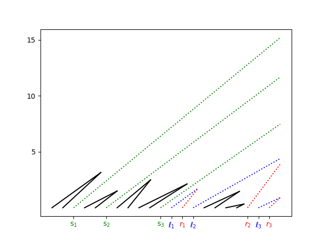
Figure 5. A bullet process with k=3 survivors, $S=\{\bullet_{s_{1}},\bullet_{s_{2}},\bullet_{s_{3}}\}$. $S_{r_{n}}=S$ for each $r_{n}$.

We can now prove half of Theorem 4.

Lemma 7.

If $v$ is slow, then $|PS_{>v}|=\infty$.

Corollary 8.

$\hat{v}\geq v_{c}$.

Proof of Corollary 8.

For any $v<v_{c}$, $v$ is slow. By Lemma 7 then, $\hat{v}\geq v$. ∎

Proof of Lemma 7.

Let $E\subset\Omega^{\mathbb{N}_{>0}}$ be the event that $|PS_{>v}|<\infty$. We show that if $\mathbf{P}(E)>0$ then $v$ is fast. Given $\vec{\bullet}\mkern 2.0mu\vphantom{\bullet}\in E$, we show $\bullet^{v}_{0}$ can survive in front of it, with a finite shield $\vec{\bullet}\mkern 2.0mu\vphantom{\bullet}_{\mathcal{J}}=(\bullet_{i_{1}},\ldots,\bullet_{i_{n}})$ in between, indexed by $\mathcal{J}=\{i_{1},\ldots,i_{n}\}=\{\frac{1}{n+1},\ldots,\frac{n}{n+1}\}$. That is, we construct a non-null event $F\subseteq\Omega^{\mathcal{J}}$ such that $\bullet^{v}_{0}$ survives in $B(\bullet^{v}_{0},\vec{\bullet}\mkern 2.0mu\vphantom{\bullet}_{\mathcal{J}},\vec{\bullet}\mkern 2.0mu\vphantom{\bullet})$ whenever $\vec{\bullet}\mkern 2.0mu\vphantom{\bullet}\in E$, and $\vec{\bullet}\mkern 2.0mu\vphantom{\bullet}_{\mathcal{J}}\in F$ (actually, we use a non-null $E^{\prime}\subset E$). $\mathbf{P}(E^{\prime}\cap F)=\mathbf{P}(E^{\prime})\,\mathbf{P}(F)>0$, so $\bullet_{0}^{v}$ can survive. Figure 6 depicts the construction of $F$.

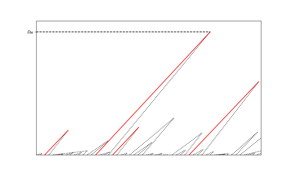
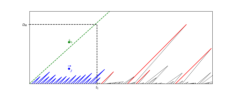
Figure 6. Above we depict $B(\vec{\bullet}\mkern 2.0mu\vphantom{\bullet})$ for $\vec{\bullet}\mkern 2.0mu\vphantom{\bullet}\in E_{0}$. $PS_{>v}$ consists of $4$ bullets, whose paths are drawn in red. Below, the path of $\bullet^{v}_{0}$ is green, and in blue is $\vec{\bullet}\mkern 2.0mu\vphantom{\bullet}_{\mathcal{J}}$, which shields $\bullet^{v}_{0}$ from its $4$ threats.

Suppose then that $PS_{>v}$ is finite. If $S\subseteq PS$ contains any bullets with velocity $\leq v$, then we already know $v$ is fast, so assume $S\subseteq PS_{>v}$, and is thus finite. We could construct $F$ to shield $\bullet^{v}_{0}$ from these survivors, but to simplify our argument we show we can further assume $|S|=0$, that is $E_{0}:=E\cap\{|S|=0\}$ is non-null. Let $\bullet_{s}$ be the last survivor in $S$. Then $\vec{\bullet}\mkern 2.0mu\vphantom{\bullet}_{[s+1,\infty)}\in E_{0}$: first off, $B_{[s+1,\infty)}$ has no survivors, as any such survivor would either survive in $B(\vec{\bullet}\mkern 2.0mu\vphantom{\bullet})$ or annihilate $\bullet_{s}$, neither of which happens. To see $\vec{\bullet}\mkern 2.0mu\vphantom{\bullet}_{[s+1,\infty)}\in E$, by Theorem 6 (1), $\bullet_{s}\in S_{n}$ for large $n$, at which point if $\bullet_{n}\in S_{[s+1,n]}$ — i.e. $\bullet_{n}\in PS_{[s+1,\infty)}$ — then $\bullet_{n}\in S_{n}$ — i.e. $\bullet_{n}\in PS$. Therefore, $PS_{[s+1,\infty)}\setminus PS$ is finite, so $(PS_{[s+1,\infty)})_{>v}$ is as well.

So take $\vec{\bullet}\mkern 2.0mu\vphantom{\bullet}\in E_{0}$. Clearly, we can ignore the case $PS_{>v}=\varnothing$, since then $\bullet_{0}^{v}$ survives in $B(\bullet_{0}^{v},\vec{\bullet}\mkern 2.0mu\vphantom{\bullet})$ as it is never threatened. Call $D_{M}$ the furthest location any member of $PS_{>v}$ ever reaches. Assuming that $\vec{\bullet}\mkern 2.0mu\vphantom{\bullet}_{\mathcal{J}}$ mutually annihilates in $B(\bullet_{0}^{v},\vec{\bullet}\mkern 2.0mu\vphantom{\bullet}_{\mathcal{J}},\vec{\bullet}\mkern 2.0mu\vphantom{\bullet})$, $\bullet^{v}_{0}$ can only be annihilated by some member of $PS_{>v}$, so the location of this collision would have to be at most $D_{M}$. $\vec{\bullet}\mkern 2.0mu\vphantom{\bullet}_{\mathcal{J}}$ serves as a time shield to allow $\bullet_{0}^{v}$ to reach $D_{M}$ and therefore survive. Let $V_{M}>v$ denote the maximum velocity in $PS_{>v}$, and choose $d_{M},v_{M}$ so that with positive probability $d_{M}\geq D_{M}$ and $v_{M}\geq V_{M}$, moreover choosing $v_{M}$ so that $\mu([v_{M},\infty))>0$. Let $E^{\prime}\subseteq E_{0}$ denote that these bounds on $D_{M},V_{M}$ are satisfied. $F$ is the event that for each $1\leq k\leq m$, $v_{i_{2k-1}}\leq v$ and $v_{i_{2k}}\geq v_{M}$, and that $\sum_{j=1}^{2m}\delta_{i_{j}}>d_{M}/v$. Note that since $PS_{>v}$ is finite, we must have $\mu([0,v])\geq 0$. Therefore $\mathbf{P}(F)>0$ for large enough $m$.

On $E^{\prime}\cap F$, $B(\bullet_{0}^{v},\vec{\bullet}\mkern 2.0mu\vphantom{\bullet}_{\mathcal{J}})$ has collisions $\bullet_{i_{2k}}\rightarrow\bullet_{i_{2k-1}}$ for $1\leq k\leq m$ and $\bullet_{0}^{v}$ survives. Since no bullet in $\vec{\bullet}\mkern 2.0mu\vphantom{\bullet}$ enters $B(\bullet_{0}^{v},\vec{\bullet}\mkern 2.0mu\vphantom{\bullet}_{\mathcal{J}},\vec{\bullet}\mkern 2.0mu\vphantom{\bullet})$ until after time $d_{M}/v$, we see that $\bullet_{0}^{v}$ makes it to distance $d_{M}$ and therefore survives provided $\vec{\bullet}\mkern 2.0mu\vphantom{\bullet}_{\mathcal{J}}$ still mutually annihilates when $\vec{\bullet}\mkern 2.0mu\vphantom{\bullet}$ is added. But we still have $\bullet_{i_{2m}}\rightarrow\bullet_{i_{2m-1}}$ in $B(\bullet_{0}^{v},\vec{\bullet}\mkern 2.0mu\vphantom{\bullet}_{\mathcal{J}},\vec{\bullet}\mkern 2.0mu\vphantom{\bullet})$ since $PS(\vec{\bullet}\mkern 2.0mu\vphantom{\bullet})_{>v_{M}}$ is empty, so $\bullet_{i_{2m}}$ is never threatened from behind. We see then that $\bullet_{i_{2m-2}}$ is never threatened behind, so $\bullet_{i_{2m-2}}\rightarrow\bullet_{i_{2m-3}}$ still occurs. Repeating this, indeed $\vec{\bullet}\mkern 2.0mu\vphantom{\bullet}_{\mathcal{J}}$ mutually annihilates. ∎

Remark 9.

We quickly state how to prove $\hat{v}=v_{c}$ in the context of the bullet problem. It remains to show $\hat{v}\leq v_{c}$. Suppose by way of contradiction that $\hat{v}>v_{c}$. We force a survivor in $(v_{c},\hat{v})$. Take $v,v^{\prime}$ with $v_{c}<v<v^{\prime}<\hat{v}$. Each member of $PS_{>v^{\prime}}$ has at least a $(v^{\prime}-v)\theta(v)>0$ chance of being followed by a survivor $\bullet_{s}$ with $v_{s}\in(v,v^{\prime})$. Since $|PS_{>v^{\prime}}|=\infty$ this eventually happens. (To rigorously show this, let $\tau_{n}$ be an increasing sequence of indices in $PS_{>v^{\prime}}$, where if $\bullet_{\tau_{n}}$ is followed by a bullet with velocity in $(v,v^{\prime})$, $\bullet_{\tau_{n+1}}$ is fired after that bullet is annihilated). But then $\bullet_{s}\in S_{n}$ for large $n$, so $\bullet_{n}\notin PS_{>v^{\prime}}$.

Remark 9 almost works for general $\mu$. For any $v>v_{c}$ with $v\in\operatorname{supp}\mu$ we have $\hat{v}\leq v$: if not, then with $N_{v}=(v-\varepsilon,v+\varepsilon)$, $\varepsilon$ chosen so that $v_{c}<N_{v}<\hat{v}$, the above argument forces a survivor with speed in $N_{v}$, using that $\mu(N_{v})\theta(v-\varepsilon)>0$. This contradicts that $\hat{v}>v+\varepsilon$. However, there is an obstacle if $\operatorname{supp}\mu$ has a gap above $v_{c}$. Take

$$v_{c}^{+}:=\inf\left(\operatorname{supp}\mu\cap\left(v_{c},\infty\right)\right).$$

$\hat{v}$ can only take values in $\{v_{c},v_{c}^{+}\}$, but if $v_{c}^{+}$ is strictly larger than $v_{c}$, we still need to rule out the possibility that $\hat{v}$ can equal $v_{c}^{+}$. To overcome this obstacle, we go through Theorem 4, starting with the following lemma.

Lemma 10.

Let $v$ be a fast speed, and let $PS_{*v}$ be of the form $PS_{>v}$, $PS_{\geq v}$, or $PS_{=v}$. If $PS_{*v}$ is infinite, then so is $S_{*v}=PS_{*v}\cap S$.

Proof.

Take any index $i$. We define an increasing sequence of stopping times $\tau_{n}\leq\infty$, agnostic to whether $|PS_{*v}|=\infty$. Let $\tau_{1}>i$ be minimal such that $\bullet_{\tau_{1}}\in PS_{*v}$, if any such $\tau_{1}>i$ exists. Otherwise let $\tau_{1}=\infty$. For $\tau_{n}<\infty$, if possible let $\bullet_{\tau_{n+1}}$ be the first bullet in $PS_{*v}$ fired after $\bullet_{\tau_{n}}$ perishes. If no such $\tau_{n+1}$ exists, that is $\bullet_{\tau_{n}}\in S_{*v}$ or there are not enough bullets in $PS_{*v}$, let $\tau_{n+1}=\infty$. $\mathbf{P}(\tau_{n+1}<\infty\mid\tau_{n}<\infty)\leq 1-\theta(v)$, so a.s. $\tau_{n}=\infty$ for large $n$. Thus either $PS_{*v}$ is finite or there is some $\bullet_{\tau_{n}}\in S_{*v}$. ∎

We obtain the following corrolary.

Corollary 11.

$v_{c}\geq\inf\mu$.

Proof.

Suppose some $v<\inf\mu$ were fast. $PS_{>v}=PS$ is infinite, so $S_{>v}$ is as well by the 10. $\bullet_{1}^{v}$ cannot survive then since $(S_{[2,\infty)})_{>v}$ is non-empty, being infinite. ∎

We now have the tools to prove there are infinite survivors when $\mu$ has finite support.

Proof of Theorem 2.

Suppose $\mu$ is supported on some finite set $V=\{V_{1},\ldots,V_{n}\}$. Then $PS_{>\hat{v}}$ is always finite, so $\hat{v}$ is fast by Lemma 7. Also, $PS_{=\hat{v}}$ is infinite, as is $S_{=\hat{v}}$ then by Lemma 10. Since the speeds of survivors are non-increasing, all but finitely many have speed $\hat{v}$.

It remains to show $\hat{v}=v_{c}$. We could appeal to Theorem 1, or alternatively let $V_{m}$ be the minimal value $\hat{v}$ takes with positive probability. Again, $V_{m}$ is fast. Each member of $PS_{>V_{m}}$ is followed by a velocity-$V_{m}$ survivor with probability $\mu(\{V_{m}\})\theta(V_{m})$. Arguing as in Remark 9 then, $PS_{>V_{m}}$ must be finite, so in fact $\hat{v}=V_{m}$. To see $V_{m}=v_{c}$, by the above, $|S_{=V_{m}}|=\infty$, so any $v<V_{m}$ is slow as it is followed by infinitely many faster survivors of $B_{[2,\infty)}$. ∎

To prove a zero-one law for $|S_{*v}|=\infty$, we first analyze the effect adding a new bullet to the front has on the set of survivors. In Section 1.5 of [BM20], the case where a bullet is added to the back is characterized. $S_{n}$ and $S_{n+1}$ differ by exactly one bullet in the following way. Let $s_{k}$ be the last bullet in $S_{n}$ (if $|S_{n}|=0$ let $s_{k}=-1$). $S_{n+1}$ equals either $S_{n}\setminus\{\bullet_{s_{k}}\}$ or $S_{n}\cup\bullet_{s_{k+1}}$, where $s_{k+1}>s_{k}$. We reproduce their argument from the front.

Lemma 12.

Take any bullets $\bullet_{0},\bullet_{1},\ldots\bullet_{n}$. If $S_{n}=S_{[1,n]}$ is non-empty, call its first bullet $\bullet_{s_{1}}$. Then $S_{[0,n]}$ is either of the form $S_{n}\setminus\{\bullet_{s_{1}}\}$ or $\{\bullet_{s_{0}}\}\cup S_{n}$ with $s_{0}<s_{1}$. If $S_{n}$ is empty then $|S_{[0,n]}|=1$.

Proof.

Let $\bullet_{1},\ldots\bullet_{f}$ be the string of non-survivors at the front of $B_{[1,n]}$, where $0\leq f\leq n$. That is, $f=s_{1}-1$ when $S_{n}$ is non-empty, and $f=n$ otherwise. We proceed by strong induction on $f$. There are three possibilities for $\bullet_{0}$ in $B_{[0,n]}$: it can survive, it can be annihilated by some $\bullet_{\ell}$ with $1\leq\ell\leq f$ as in Figure 7, or it can be annihilated by $\bullet_{s_{1}}$. In the first scenario, $S_{[0,n]}=\{\bullet_{0}\}\cup S_{n}$, and in the third scenario $S_{[0,n]}=S_{n}\setminus\{\bullet_{s_{1}}\}$. The remaining case is when $\bullet_{\ell}\rightarrow\bullet_{0}$ in $B_{[0,n]}$, whereas in $B_{[1,n]}$ we have $\bullet_{r}\rightarrow\bullet_{\ell}$ for some $\ell<r\leq f$. The collision between $\bullet_{0}$ and $\bullet_{\ell}$ frees up $\bullet_{r}$, so $S_{[0,n]}=S_{[r,n]}$ while $S_{n}=S_{[r+1,n]}$. By strong induction we are done, since $B_{[r+1,n]}$ has $f-r<f$ non-survivors at the front. ∎

Figure 7. $B_{n}$ with two survivors, $\bullet_{s_{1}}$ and $\bullet_{s_{2}}$. $\bullet_{\ell}$ is one of the bullets that can potentially annihilate $\bullet_{0}$.

Lemma 13.

Let $S_{*v}$ be of the form $S_{>v}$, $S_{\geq v}$, or $S_{=v}$. Then $\mathbf{P}(|S_{*v}|=\infty)\in\{0,1\}$.

Proof.

Suppose $\mathbf{P}(|S_{*v}|=\infty)>0$. By Birkhoff’s Ergodic Theorem then, there is some $k$ with $|(S_{[k,\infty)})_{*v}|=\infty$. Enumerate $S_{[k,\infty)}=\{\bullet_{s_{1}},\bullet_{s_{2}},\ldots\}$ with $k\leq s_{1}<s_{2}<\ldots$. We show $\bullet_{s_{i}}\in S$ for $i\geq k$. By Theorem 6 (1), $\{\bullet_{s_{1}},\ldots\bullet_{s_{i}}\}\in S_{[k,n]}$ for large $n$. By Lemma 12, $\{\bullet_{s_{2}},\ldots\bullet_{s_{i}}\}\in S_{[k-1,n]}$. Applying Lemma 12 again we get $\{\bullet_{s_{3}},\ldots\bullet_{s_{i}}\}\in S_{[k-2,n]}$. Repeating this $k-1$ times, $\{\bullet_{s_{k}},\ldots\bullet_{s_{i}}\}\in S_{[1,n]}=S_{n}$ for large $n$. By Theorem 6 again then, $\{\bullet_{s_{k}},\ldots\bullet_{s_{i}}\}\subset S$. ∎

Corollary 14.

$\mathbf{P}(|S|=\infty)\in\{0,1\}$.

Proof.

This is a direct consequence of Lemma 13 since $S=S_{\geq 0}$. ∎

We can now prove our main theorems.

Proof of Theorem 4.

Take $v$ with $\mathbf{P}(|PS_{>v}|=\infty)>0$. By Lemmas 10 and 13, $|S_{>v}|=\infty$ a.s. Then $v$ is slow, since $(S_{[2,\infty)})_{>v}$ is never empty. ∎

Proof of Theorem 1.

Any $v>v_{c}$ is fast, so $\hat{v}\leq v$ by Theorem 4. Corollary 8 is the other direction. ∎

Finally, we establish our continuity results.

Proof of Theorem 3.

1. Right-continuity of $\theta$ follows straightforwardly from the definition of the bullet process. Whenever $\bullet_{1}^{v}$ perishes, so does $\bullet_{1}^{u}$ for slightly faster $u$.

   More precisely, $\theta(v)=\mathbf{P}(A_{v})$ where $A_{v}$ denotes the event that $\bullet_{1}^{v}$ survives in $B(\bullet_{1}^{v},\vec{\bullet}\mkern 2.0mu\vphantom{\bullet}_{[2,\infty)})$. So for $u>v$, $\theta(u)-\theta(v)=\mathbf{P}(A_{u}\setminus A_{v})$. For fixed $\vec{\bullet}\mkern 2.0mu\vphantom{\bullet}$, let $v_{m}\in[0,\infty]$ be the infimum over $v^{\prime}$ for which $\vec{\bullet}\mkern 2.0mu\vphantom{\bullet}\in A_{v^{\prime}}$, so $A_{u}\subseteq\{v_{m}\leq u\}$. Take some $\vec{\bullet}\mkern 2.0mu\vphantom{\bullet}\in A_{v}^{c}$. Then $\bullet_{1}^{v}$ is involved in some collision $\bullet_{r}\rightarrow\bullet_{1}^{v}$ at some time $t$. Since triple collisions do not occur, as in Figure 8 we still have $\bullet_{r}\rightarrow\bullet_{1}^{v^{\prime}}$ for slightly faster $v^{\prime}$, as $\bullet_{r}$ survives to at least some $t^{\prime}>t-\delta_{1}$ in $B_{[2,\infty)}$. Therefore, $v_{m}$ is strictly larger than $v$. As $u\searrow v$ then, $\theta(u)-\theta(v)\leq\mathbf{P}(A_{v}^{c},v_{m}\leq u)\to 0$.

   

   Figure 8. $\bullet_{1}^{v}$’s path is drawn in solid blue, and $\bullet_{r}$’s in red. $\bullet_{1}^{v^{\prime}}$ is drawn in dotted blue. It still collides with $\bullet_{r}$ since there are no triple collisions.

2. Take $v>v_{c}$. First suppose $\mu(\{v\})>0$. Let $E$ be the event that $v_{2}=v$ and $\bullet_{2}\in S_{[2,\infty)}$, so $\mathbf{P}(E)=\mu(\{v\})\theta(v)>0$. For any $u<v$, $E\subseteq A_{v}\setminus A_{u}$, so $\theta(v)-\theta(u)\geq\mathbf{P}(E).$

   Now suppose $v$ is not an atom of $\mu$. We need to show left-continuity. Take some $\vec{\bullet}\mkern 2.0mu\vphantom{\bullet}\in A_{v}$. If $S_{[2,\infty)}$ is non-empty, let its first and fastest bullet have speed $v^{\prime}$. $v^{\prime}$ cannot be faster than $v$, and is almost surely slower. If $S_{[2,\infty)}=\varnothing$, simply let $v^{\prime}$ be the midpoint of $[v_{c},v]$. As $v^{\prime}$ is fast, $(PS_{[2,\infty)})_{>v^{\prime}}$ is finite, and all its bullets die. Enumerate $(PS_{[2,\infty)})_{>v^{\prime}}=(\bullet_{j_{1}},\ldots\bullet_{j_{n}})$. These are the only bullets that could possibly threaten $\bullet_{1}^{u}$ for any $u\in[v^{\prime},v]$. Now each $\bullet_{j_{k}}$ perishes in $B(\bullet_{1}^{v},\vec{\bullet}\mkern 2.0mu\vphantom{\bullet}_{[2,\infty)})$, and so is involved in some collision at time $t_{j_{k}}$ and location $d_{j_{k}}$. $\bullet^{v}_{1}$ avoids this collision by advancing to some $d^{\prime}_{j_{k}}>d_{j_{k}}$ at time $t_{j_{k}}$, as would $\bullet^{u_{k}}_{1}$ for a slightly slower $u_{k}<v$. Then $v_{m}$ is at most the maximum of these $u_{k}$. Most importantly, $v_{m}<v$ a.s. So for $u<v$, $\theta(v)-\theta(u)\leq\mathbf{P}(A_{v},v_{m}\geq u)\to 0$ as $u\nearrow v$.

3. With right-continuity established, continuity at $v_{c}$ is equivalent to $\theta(v_{c})=0$, so the result follows from Theorem 4.

∎

References

- [BM20] Nicolas Broutin and Jean-François Marckert, The combinatorics of the colliding bullets, Random Structures Algorithms 56 (2020), no. 2, 401–431. MR 4060351
- [DKJ+19] Brittany Dygert, Christoph Kinzel, Matthew Junge, Annie Raymond, Erik Slivken, and Jennifer Zhu, The bullet problem with discrete speeds, Electron. Commun. Probab. 24 (2019), Paper No. 27, 11. MR 3962477
- [EF85] Yves Elskens and Harry L. Frisch, Annihilation kinetics in the one-dimensional ideal gas, Phys. Rev. A 31 (1985), 3812–3816.
- [KW14] Michael Kleber and David Wilson, “Ponder This” IBM research challenge, https://research.ibm.com/haifa/ponderthis/challenges/May2014.html, 2014.
- [ST17] Vladas Sidoravicius and Laurent Tournier, Note on a one-dimensional system of annihilating particles, Electron. Commun. Probab. 22 (2017), Paper No. 59, 9. MR 3718709