Scalable and Explainable Verification of Image-based Neural Network Controllers for Autonomous Vehicles

Abstract.

Existing formal verification methods for image-based neural network controllers in autonomous vehicles often struggle with high-dimensional inputs, computational inefficiency, and a lack of explainability. These challenges make it difficult to ensure safety and reliability, as processing high-dimensional image data is computationally intensive and neural networks are typically treated as black boxes. To address these issues, we propose SEVIN (Scalable and Explainable Verification of Image-Based Neural Network Controllers), a framework that leverages a Variational Autoencoders (VAE) to encode high-dimensional images into a lower-dimensional, explainable latent space. By annotating latent variables with corresponding control actions, we generate convex polytopes that serve as structured input spaces for verification, significantly reducing computational complexity and enhancing scalability. Integrating the VAE’s decoder with the neural network controller allows for formal and robustness verification using these explainable polytopes. Our approach also incorporates robustness verification under real-world perturbations by augmenting the dataset and retraining the VAE to capture environmental variations. Experimental results demonstrate that SEVIN achieves efficient and scalable verification while providing explainable insights into controller behavior, bridging the gap between formal verification techniques and practical applications in safety-critical systems.

1. Introduction

Ensuring the safety and reliability of image-based neural network controllers in autonomous vehicles (AVs) is paramount. These controllers process high-dimensional inputs, such as images from front cameras, to make real-time control decisions. However, existing formal verification methods (Katz et al., 2017a; Gehr et al., 2018; Singh et al., 2019) face significant challenges due to the high dimensionality and complexity of image inputs, leading to computational inefficiency and scalability issues (Bunel et al., 2018; Singh et al., 2018). Moreover, these methods often treat neural networks as black boxes, offering limited explainability and making it difficult to understand how specific inputs influence outputs—an essential aspect for safety-critical applications like AVs.

Recent efforts have employed abstraction-based methods (Gehr et al., 2018; Singh et al., 2019) and reachability analysis (Ruan et al., 2018) to approximate neural network behaviors. Specification languages grounded in temporal logic (Pnueli, 1977; Vasilache et al., 2022) and Satisfiability Modulo Theory (SMT) solvers (Ehlers, 2017) have been used to formalize and verify properties. However, these approaches often struggle with scalability and explainability when applied to high-dimensional input spaces inherent to image-based controllers.

Furthermore, robustness verification under real-world input perturbations remains challenging. Modeling and analyzing such variations efficiently is difficult due to the complexity of image data and environmental factors affecting AVs. Consequently, current approaches lack methods that:

• Reduce Computational Complexity: Effectively handle the high dimensionality of image inputs without compromising verification thoroughness.

• Enhance Interpretability: Provide insights into how input features influence control actions, facilitating better understanding and trust.

• Improve Scalability: Scale to larger datasets and more complex controllers, especially when considering robustness against real-world perturbations.

To address these limitations, we propose SEVIN (Scalable and Explainable Verification of Image-Based Neural Network Controllers), a novel approach that leverages unsupervised learning with a Variational Autoencoder (VAE) (Kingma and Welling, 2013) to learn a structured latent representation of the controller’s input space. By encoding high-dimensional image data into a lower-dimensional, explainable latent space, we significantly reduce the computational complexity of the verification process, making it more scalable.

Our method involves training a VAE on a dataset of image-action pairs collected from a driving simulator. The latent space is partitioned into convex polytopes corresponding to different control actions, enabling us to define formal specifications over these polytopes. By operating in this latent space, we enhance explainability and gain insights into how latent features influence control actions.

We further extend our approach to incorporate robustness verification under input perturbations common in real-world scenarios for AVs. By augmenting the dataset with perturbed images and retraining the VAE, we ensure that the latent space captures variations due to environmental changes, sensor noise, and other factors affecting image inputs.

Our experimental results demonstrate that SEVIN not only achieves efficient and scalable verification of image-based neural network controllers but also provides explainable insights into the controller’s behavior. This advancement bridges the gap between formal verification techniques and practical applications in safety-critical systems like AVs. In summary, we make the following contributions

1.1. Summary of Contributions

• An explainable latent space is developed for a neural network controller dataset by employing a Gaussian Mixture-VAE model. The encoded variables are annotated according to the control actions correlated with their high-dimensional inputs, enabling the derivation of convex polytopes as defined input spaces for the verification process.

• A streamlined and scalable framework is then constructed to integrate the VAE’s decoder network with the neural network controller, facilitating formal and robustness verification of the controller by utilizing the explainable convex polytopes as structured input spaces.

• Finally, symbolic specifications are synthesized to encapsulate the safety and performance properties of two image-based neural network controllers. Leveraging these specifications in conjunction with the $\alpha-\beta-CROWN$ neural network verification tool (Authors, 2023), formal and robustness verification of the controllers is effectively conducted.

2. Preliminaries

2.1. Variational Autoencoder (VAE)

VAEs are generative models that compress input data ($\mathbf{x}$) into a latent space and then reconstruct the input from this latent representation ($\mathbf{\hat{x}}$) (Kingma and Welling, 2013; Rezende et al., 2014). A VAE $V(\mathbf{x})$, consists of an encoder $E(\mathbf{x})$ and a decoder $D(\mathbf{z})$, where $\mathbf{z}$ is the latent variable capturing the compressed representation of the input data.

In variational inference, the true posterior distribution $p(\mathbf{z}|\mathbf{x})$ is often intractable to compute directly and hence an approximate posterior $q(\mathbf{z}|\mathbf{x})$ is introduced(Kingma and Welling, 2013). The encoder maps the input data to a latent distribution $q_{\phi}(\mathbf{z}|\mathbf{x})$, parameterized by $\phi$, while the decoder reconstructs the input data from the latent variable using $p_{\theta}(\mathbf{x}|\mathbf{z})$, parameterized by $\theta$. Instead of directly calculating for the intractable marginal likelihood $p(\mathbf{x})$, VAEs maximize the Evidence Lower Bound (ELBO) to provide a tractable lower bound to $\log p(\mathbf{x})$ (Kingma and Welling, 2013):

(1) $$\text{ELBO}=\underbrace{\mathbb{E}_{\mathbf{z}\sim q_{\phi}(\mathbf{z}|\mathbf{x})}[\log p_{\theta}(\mathbf{x}\ |\ \mathbf{z})]}_{\text{Reconstruction Term}}-\underbrace{\mathcal{D}_{KL}[q_{\phi}(\mathbf{z}\ |\ \mathbf{x})\,\|\,p(\mathbf{z})]}_{\text{KL Divergence Term}}$$

The ELBO consists of a reconstruction term that encourages the decoded output to be similar to the input data, and a Kullback-Leibler (KL) divergence term that regularizes the latent space to match a prior distribution $p(\mathbf{z})$. The prior $p(\mathbf{z})$ is often chosen as a standard Gaussian (Kingma and Welling, 2013), but can be more flexible, such as a Gaussian mixture model (Dilokthanakul et al., 2016) or VampPrior (Tomczak and Welling, 2018), depending on the desired latent space structure.

2.2. Neural Network Verification

Neural network verification tools are designed to rigorously analyze and prove properties of neural networks, ensuring that they meet specified input-output requirements under varying conditions (Liu et al., 2019). Consider an $L$-layer neural network representing the function $F(\mathbf{x})$ for which the verification tools can determine the validity of the property as:

(2) $$\mathbf{x}\in X\implies F(\mathbf{x})\in A$$

where $X$ and $A$ are the convex input and output sets, respectively  (Katz et al., 2017b). The neural network verification ensures that for all inputs in a specified set $X$, the outputs of the neural network $F(\mathbf{x})$ satisfy certain properties defined by a set $A$. The weights and biases for $F(\mathbf{x})$ are represented as $\mathbf{W}^{(i)}\in\mathbb{R}^{d_{n}^{(i)}\times d_{n}^{(i-1)}}$ and $\mathbf{b}^{(i)}\in\mathbb{R}^{d_{n}^{(i)}}$, where $d_{n}^{(i)}$ is the dimensionality for layer $i\in\{1,\ldots,L\}$ for the $L$-layered neural network. The neural network function $F(\mathbf{x})=h^{(L)}(\mathbf{x})$:

(3) $$h^{(i)}(\mathbf{x}) =\mathbf{W}^{(i)}\hat{h}^{(i-1)}(\mathbf{x})+\mathbf{b}^{(i)},$$

$$\hat{h}^{(i)}(\mathbf{x}) =\sigma\left(h^{(i)}(\mathbf{x})\right),$$

$$\hat{h}^{(0)}(\mathbf{x}) =\mathbf{x}$$

where $\sigma$ denotes the activation function. When the ReLU activation function is used, the neural network verification problem (2) becomes a constrained optimization problem with the objective function as shown below (Tjeng et al., 2019),

(4) $$F_{\min}=\min_{\mathbf{x}\in X}F(\mathbf{x}),\quad F_{\max}=\max_{\mathbf{x}\in X}F(\mathbf{x})$$

s.t. $$F_{\min},F_{\max}\in A$$

where $F(\mathbf{x})$ is defined as the set of piecewise-linear functions from Equation (3). Since the ReLU activation functions are piecewise linear, allowing the neural network to be represented as a combination of linear functions over different regions of the input space, the verification problem can be formulated as an optimization problem solvable by techniques such as Mixed-Integer Linear Programming (MILP) (Tjeng et al., 2019) and SMT solvers (Kaiser et al., 2021).

Furthermore, robust formal verification is a specific aspect of neural network verification that focuses on the network’s resilience to small perturbations in the input data (Huang et al., 2017). The robustness verification problem can be formalized as:

$$\mathbf{x}\in B(\mathbf{x}_{0},\delta)\implies F(\mathbf{x})\in A$$

where $B(\mathbf{x}_{0},\delta)=\{\mathbf{x}|\|\mathbf{x}-\mathbf{x}_{0}\|\leq\delta\}$ represents a norm-bounded perturbation around a nominal input $\mathbf{x}_{0}$, and $\delta>0$ is the perturbation limit. Alternatively, robustness verification can also be formulated as a constrained optimization problem:

(5) $$F_{\min}=\min_{\mathbf{x}\in B(\mathbf{x}_{0},\delta)}F(\mathbf{x}),\quad F_{\max}=\max_{\mathbf{x}\in B(\mathbf{x}_{0},\delta)}F(\mathbf{x})$$

s.t. $$F_{\min},F_{\max}\in A$$

By solving the optimization problems in (4) and (5) within their defined input sets, and verifying that the corresponding outputs reside within the target set $A$, verification tools such as Reluplex (Katz et al., 2017a) and AI² (Gehr et al., 2018) provide essential guarantees for vanilla formal and robustness verification.

Figure 1. The SEVIN model can be decomposed into two sub-modules for conducting formal verification of any neural network controller. (a) A VAE, defined as $\hat{\mathbf{x}}=D(E(\mathbf{x}))$, is initially trained and utilized to learn representation sets ($Z_{i}$) of latent features from the dataset $X$. The same dataset $X$ is also used to train the image-based neural network controller $F(\mathbf{x})$, which will later undergo verification. (b) Any latent feature sample $\mathbf{z}\in Z_{i}$ is representative of the dominant features that influence the control action ($\mathbf{a}$) predicted by $F(\mathbf{x})$. By combining the decoder $D(\mathbf{z})$ with the neural network controller $F(\mathbf{x})$, we can determine a set of control actions $A_{i}$ based on $Z_{i}$ (see more in Lemma 1). Finally, using a neural network verification tool, we can formally verify the satisfaction of the neural network controller $F(\mathbf{x})$ with against a formal specification ($\phi$)

2.3. Symbolic Specification Language

The symbolic specification language defines properties for neural network verification, integrating principles from Linear Temporal Logic (LTL) (Pnueli, 1977) to express dynamic, time-dependent behaviors essential for cyber-physical systems like AV.

LTL formulas are defined recursively as:

$$\Phi::=\text{true}|a|\varphi_{1}\lor\varphi_{2}|\neg\varphi|\bigcirc\varphi|\varphi_{1}\,\mathcal{U}\,\varphi_{2}$$

where

• true denotes the Boolean constant True.

• $a$ is an atomic proposition, typically about network inputs or outputs.

• $\lor$, $\neg$, $\bigcirc$, and $\mathcal{U}$ represent disjunction, negation, next, and until operators.

Using the above LTL formulas, other operators like “always” ($\square\varphi$) and “eventually” ($\lozenge\varphi$) can be defined $\square\varphi\equiv\neg\lozenge\neg\varphi,\lozenge\varphi\equiv\text{true}\,\mathcal{U}\,\varphi.$

These temporal operators allow precise specification of properties over time, such as safety ($\square\varphi$) and liveness ($\lozenge\varphi$) conditions. Specification methods based on LTL (Pnueli, 1977; Vasilache et al., 2022), Signal Temporal Logic (STL) (Akazaki and Liu, 2018), Satisfiability Modulo Theories (SMT) (Ehlers, 2017), and other formal techniques provide the basis for rigorous neural network verification, enabling precise and reliable analysis of temporal behaviors in dynamic environments.

Example 0.

Consider an image based neural network controller $F(\mathbf{x})$ that is trained to predict steering action values ($\mathbf{a}$). We expect that for all images in the subset of left-turn images $X_{\text{left}}$, the controller should predict negative action values corresponding to turning left, i.e.,

$$\mathbf{x}\in X_{\text{left}}\implies F(\mathbf{x})\in A_{\text{left}}$$

Formal verification of the neural network $F(\mathbf{x})$ thus corresponds to solving the following optimization problem:

$$F_{\min}=\min_{\mathbf{x}\in X_{\text{left}}}F(\mathbf{x}),F_{\max}=\max_{\mathbf{x}\in X_{\text{left}}}F(\mathbf{x})$$

s.t. $$F_{\min},F_{\max}\in A_{\text{left}}$$

We can thus formally define the input specification to the neural network verification tool using the symbolic specification language operators as:

$$\varphi:=\square(\ \{F_{\min},F_{\max}\}\in A_{\text{left}})$$

If the verification tool can show that the specification $\varphi$ stands true for the given input set $X_{\text{left}}$, then the specification is satisfied (SAT), or else the specification is unsatisfied (UNSAT).

3. Problem Formulation

Ensuring the safety and reliability of image-based neural network controllers in AVs is paramount. Existing verification methods, however, face significant challenges due to the high dimensionality and complexity of image inputs, leading to computational inefficiency (Gehr et al., 2018; Singh et al., 2018; Bunel et al., 2018). These methods often lack explainability, treating neural networks as black boxes with limited insight into how inputs influence outputs, which is critical for safety-critical applications like AVs. Additionally, robustness verification under real-world input perturbations remains difficult due to the complexity of modeling and analyzing such variations efficiently. Consequently, current approaches struggle with explainability, computational complexity, and scalability.

3.1. Our Solution

We begin by collecting images and control actions from a driving simulator, forming a dataset of image-action pairs $(\mathbf{x},\mathbf{a})$, where $X=\{\mathbf{x}_{j}\}_{j=1}^{N}$ consists of $N$ front camera images and $A=\{\mathbf{a}_{j}\}_{j=1}^{N}$ consists of the corresponding control actions. A VAE $V(\mathbf{x})$ is trained to learn the latent representation $Z$ of this dataset, encoding high-dimensional image data into a lower-dimensional latent space (see Section 4.1). This encoding reduces the computational complexity of the verification problem, making it more scalable.

Once the VAE is trained, we label the latent variables ($\mathbf{z}$) based on their corresponding control actions ($\mathbf{a}$). This labeling allows us to partition the latent space $Z$ into convex polytopes $C_{i}$, such that $C=\bigcup_{i\in I}C_{i}$, as elaborated in Section 4.3. Each polytope $C_{i}$ corresponds to a specific control action set $A_{i}$, with the action space expressed as $A=\bigcup_{i\in I}A_{i}$. This partitioning generates an explainable input space for the formal verification process, enhancing the understanding of how inputs influence outputs.

We then split the trained VAE into encoder $E(\mathbf{x})$ and decoder $D(\mathbf{z})$ networks and concatenate the decoder with the controller network $F(\mathbf{x})$. The combined network $\mathcal{H}(\mathbf{z})=F(D(\mathbf{z}))$ maps variables directly from the latent space to control actions. By operating in the latent space instead of the high-dimensional image space, we significantly reduce the input dimensionality and computational complexity of the verification problem, making the process more scalable and computationally efficient.

Formal specifications $\varphi$ are defined using the symbolic specification language described in Section 2.3, capturing the safety and performance properties of the neural network controller $F(\mathbf{x})$. The combined network $\mathcal{H}(\mathbf{z})$ and the specifications $\varphi$ are provided to a neural network verification tool, such as $\alpha$-$\beta$-CROWN (Authors, 2023), which uses bound propagation and linear relaxation techniques to certify properties of neural networks. The verification tool checks whether $\mathcal{H}(\mathbf{z})$ satisfies the specifications $\varphi$ over the input convex polytopes in the latent space. The equivalence between verifying $F(\mathbf{x})$ and $\mathcal{H}(\mathbf{z})$ is established in Theorem 4.

To address robustness verification under input perturbations common in real-world scenarios, we extend our approach by training the VAE on a dataset of both clean and augmented images (see Section 4.5). The augmented dataset $\bar{X}$ is generated by applying quantifiable perturbations—such as changes in brightness, rotations, translations, and motion blurring—to the original images (see Figure 4). The corresponding latent representation set $\bar{Z}$ is used by SEVIN to generate augmented latent space convex polytopes $\bar{C}_{i}$ for robustness analysis. The overall formal verification process aims to assess the neural network controller’s performance under two distinct conditions:

Vanilla formal verification: for a clean input space $C_{i}$, drawn from the subset $X_{i}\subseteq X$, assumed to consist of unperturbed, front-camera-captured images.

Robust formal verification: based on an augmented input space $\bar{C}_{i}$ from the subset $\bar{X_{i}}\subseteq\bar{X}$, where $\bar{X}$ comprises images with applied, quantifiable augmentations relevant to AV scenarios.

This extension makes the verification process more scalable by incorporating robustness verification into the same framework without significant additional computational complexity.

4. Scalable and Explainable Verification of Image-based Neural Networks (SEVIN)

4.1. Latent Representation Learning of the Dataset

To develop a scalable and explainable framework for neural network controller verification, we first train a VAE on the dataset of images used in the neural network controller training process. The VAE is tasked with reconstructing front-camera images captured by an AV while learning latent representations that capture the underlying structure and variability in the data—such as different driving conditions, environments, and vehicle behaviors—in a compressed and informative form.

Let $V(\mathbf{x}):\mathbb{R}^{h\times w}\rightarrow\mathbb{R}^{h\times w}$ represent a Gaussian Mixture Variational Autoencoder (GM-VAE) trained over a dataset of images $X=\{\mathbf{x}_{i}\}_{i=1}^{M}\subset\mathbb{R}^{h\times w}$ to learn a structured latent space representation $\mathbf{z}\in Z\subset\mathbb{R}^{d_{z}}$ and reconstruct images $\hat{\mathbf{x}}=V(\mathbf{x})\in\hat{X}\subset\mathbb{R}^{h\times w}$. Here, $h\times w$ denotes the height and width of the images. We assume a Gaussian mixture prior over the latent variables $\mathbf{z}$, defined as:

(6) $$p(\mathbf{z})=\sum_{k=1}^{K}s_{k}\,\mathcal{N}(\mathbf{z}|\boldsymbol{\mu}_{k},\boldsymbol{\Sigma}_{k})$$

where $\boldsymbol{\mu}_{k}$ and $\boldsymbol{\Sigma}_{k}$ represent the mean and covariance matrix of the $k$-th Gaussian component in the latent space, and $s_{k}$ represents the mixture weight for each Gaussian, satisfying $\sum_{k=1}^{K}s_{k}=1$. The VAE $V(\mathbf{x})$ comprises an encoder model $E(\mathbf{x}):\mathbb{R}^{h\times w}\rightarrow\mathbb{R}^{3\times K\times d_{z}}$ and a decoder model $D(\mathbf{z}):\mathbb{R}^{d_{z}}\rightarrow\mathbb{R}^{h\times w}$. The encoder $E(\mathbf{x})$ outputs a $\{3\times K\times d_{z}\}$ dimensional array, where $[\boldsymbol{\mu}_{k},\log\boldsymbol{\Sigma}_{k},s_{k}]$ corresponds to the $k$-th Gaussian in every latent dimension. The variable $d_{z}$ denotes the dimensionality of the latent space. An advantage of using a GM-VAE is that it provides a more flexible latent space representation compared to a standard VAE, especially when the data exhibit multiple modes (Dilokthanakul et al., 2016).

To train the GM-VAE loss function ($\mathcal{L}$), we employ the loss function defined in (Dilokthanakul et al., 2016) as:

$$\mathcal{L}=\ \operatorname{MSE}\left(\mathbf{x},\hat{\mathbf{x}}\right)+\beta\sum_{k=1}^{K}\,\mathcal{D}_{KL}\left[q(\mathbf{z}|\mathbf{x},k)\,\|\,p(\mathbf{z},k)\right]$$

The Mean Squared Error (MSE) between the input data and the reconstructed images is used to calculate the reconstruction loss described in (1). Maximizing the likelihood $p(\mathbf{x}|\mathbf{z})$ under the Gaussian mixture is equivalent to minimizing the MSE between $\mathbf{x}$ and $\hat{\mathbf{x}}$, as the negative log-likelihood of a Gaussian distribution with fixed variance simplifies to MSE loss (Kingma and Welling, 2013). Here, $q_{\phi}(\mathbf{z}|\mathbf{x},k)$ is the posterior probability of selecting the $k$-th component of the mixture for input $\mathbf{x}$, and the KL divergence term $\mathcal{D}_{KL}$ measures the discrepancy between the posterior and the corresponding prior Gaussian component $p(\mathbf{z},k)$. The hyper-parameter $\beta\in\mathbb{R}^{+}$ balances the trade-off between reconstructing the input data accurately and minimizing the divergence between the approximate posterior and the prior distribution, similar to the concept introduced in the $\beta$-VAE framework (Higgins et al., 2017). This formulation allows the VAE to learn more complex latent structures by capturing multi-modal distributions in the latent space (Dilokthanakul et al., 2016; Kingma and Welling, 2013).

Assumption 1.

Given a GM-VAE $V(\mathbf{x})$ trained on a dataset of images $X$, we assume that the reconstructed images $\hat{\mathbf{x}}=V(\mathbf{x})$ satisfy $\|F(\hat{\mathbf{x}})-F(\mathbf{x})\|_{2}\leq\epsilon$, where $\epsilon>0$.

For a given neural network controller $F(\mathbf{x})$, the parameter $\epsilon$ is a measurable quantity that depends solely on the training efficacy of $V(\mathbf{x})$. Our objective is to optimize $V(\mathbf{x})$ to achieve $\epsilon\approx\frac{1}{100}\|F(\mathbf{x})\|_{2}$, which is considered an acceptable error threshold in our AV driving scenarios.

4.2. Explainable Latent Space Encoding

The encoder $E(\mathbf{x})$ learns a mapping from high-dimensional images $\mathbf{x}$ to low-dimensional latent representations $\mathbf{z}$. Images with similar features—such as lane markings, traffic signs, or attributes like brightness and blur—are mapped close together in the latent space because the encoder learns to associate these common attributes with nearby regions. The continuity of the latent space enforced by the KL divergence ensures that similar inputs have similar latent representations. The decoder $D(\mathbf{z})$ regenerates the front-camera images $\hat{\mathbf{x}}$ from the latent variables $\mathbf{z}\in Z$.

In our approach, each image $\mathbf{x}$ is associated with a corresponding control action $\mathbf{a}$, such as steering angle or linear velocity, which acts as a label for the image for training purposes. The control action $\mathbf{a}$ is the action to be predicted by the neural network controller $F(\mathbf{x})$ based on the image $\mathbf{x}$. The dataset $X$ collected from driving simulations is randomly split 70/30 for training and validating the VAE $V(\mathbf{x})$ and the neural network controller $F(\mathbf{x})$ respectively. The datasets are generated and labeled automatically during simulation, where the vehicle’s control actions are recorded alongside the images captured. Further details on the data collection process are provided in Section 5.1. The proof for the Lemma  1 is provided in the Appendix A.1

Lemma 0.

Let $X=\{\mathbf{x}_{i}\}_{i=1}^{M}$ be a dataset of images, and let $A\subset\mathbb{R}^{m}$ be a set of action values, where each image $\mathbf{x}_{i}$ is associated with a control action $\mathbf{a}_{i}\in A$ that the neural network controller $F(\mathbf{x})$ should predict.

Using the encoder $E(\mathbf{x})$, the images are mapped to latent variables $\mathbf{z}_{i}=E(\mathbf{x}_{i})$, resulting in the set of latent variables $Z=\{\mathbf{z}_{i}\}_{i=1}^{M}$. The latent variables are assumed to follow the GM prior distribution described in (6). Then, for each action value $\mathbf{a}\in A$, the set of latent variables corresponding to $\mathbf{a}$ has positive probability under $p(\mathbf{z})$. Specifically, the probability of sampling a latent variable $\mathbf{z}$ such that there exists a pair $(\mathbf{z},\mathbf{a})$ in $Z\times A$ is greater than zero:

(7) $$\forall\mathbf{a}\in A,\quad p\left(\exists\mathbf{z}\in Z\ \text{s.t.}\ (\mathbf{z},\mathbf{a})\in Z\times A\right)>0$$

The aim was to show that there is a non-zero probability of sampling a corresponding $\mathbf{z}$ such that the pair ($\mathbf{z,a}$) exists in the latent space. This allows us to sample variables in the latent space with the corresponding action value acting as their labels. Figure 2 illustrates the 8-dimensional latent space of the image dataset $X$, where each point is labeled according to its corresponding action value set $A_{i}$. The latent space has been reduced to 2 dimensions using t-SNE (t-distributed Stochastic Neighbor Embedding) for visualization. t-SNE is a dimensionality reduction technique that transforms high-dimensional data into a lower-dimensional space while preserving the structure of data clusters, making it ideal for visualization (van der Maaten and Hinton, 2008). Due to the clustering nature of the VAE, the latent variables with similar features are clustered and can be interpreted by their action values.

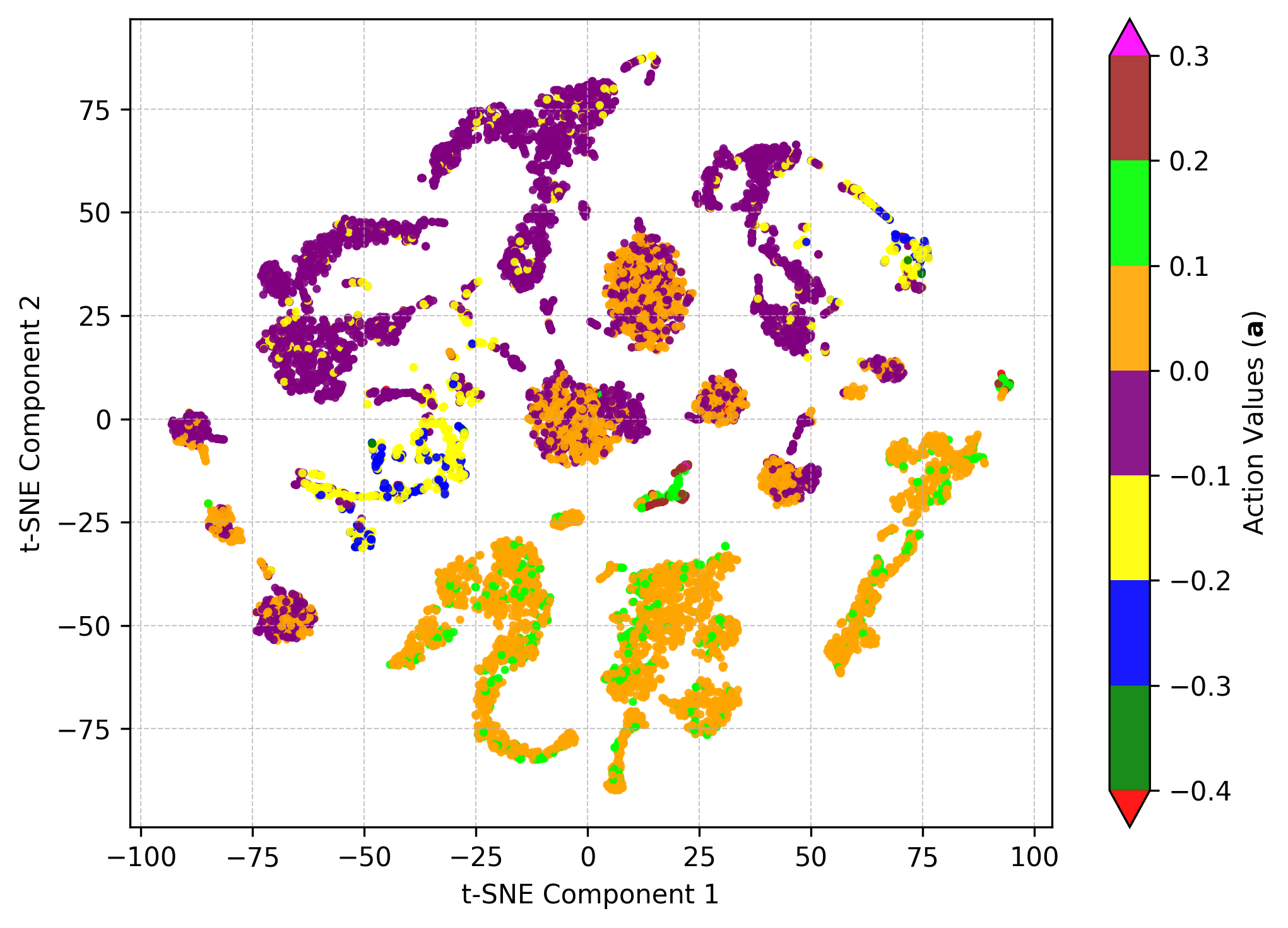
Figure 2. t-SNE plot of an 8D latent space representation generated for the clean image dataset ($X$)

4.3. Latent Space Convex Polytope Formulation

For a collection of continuous action subsets $\{A_{i}\}_{i\in I}$, where $I$ is an index set and $A=\bigcup_{i\in I}A_{i}$ covers the entire action space, we construct corresponding convex polytopes $C_{i}\subset\mathbb{R}^{d_{z}}$ in the latent space. These polytopes approximate the regions associated with each action subset $A_{i}$. To generate $C_{i}$ for a given action subset $A_{i}$, we perform Monte Carlo sampling of the latent variables $\mathbf{z}$ from the GM prior $p(\mathbf{z})$, focusing on samples corresponding to $A_{i}$. Specifically, for each $A_{i}$, we consider the set of images $X_{i}\subseteq X$ such that each image $\mathbf{x}\in X_{i}$ is associated with an action $\mathbf{a}\in A_{i}$, i.e.,

$$X_{i}=\left\{\mathbf{x}\in X\mid F(\mathbf{x})\in A_{i}\right\}$$

Using the encoder $E(\mathbf{x})$, we map the images $\mathbf{x}\in X_{i}$ to their latent representations $\mathbf{z}$, resulting in latent variables $\mathbf{z}\in Z_{i}$, where $Z_{i}$ denotes the set corresponding to $A_{i}$. This establishes the correspondence between image-action pairs $(\mathbf{x},\mathbf{a})$ and latent-action pairs $(\mathbf{z},\mathbf{a})$. To construct $C_{i}$, we draw $n$ independent samples of the latent variable $\mathbf{z}$ from the GM prior $p(\mathbf{z})$, ensuring that each sample belongs to $Z_{i}$ corresponding to $A_{i}$ and is within $2$ standard deviations from the mean $\boldsymbol{\mu}_{A_{i}}$ of $p(\mathbf{z}|\mathbf{z}\in Z_{i})$. The convex polytope $C_{i}$ is then defined as the convex hull of these sampled latent variables:

(8) $$C_{i}=\operatorname{conv}\left(\left\{\mathbf{z}_{j}|\mathbf{z}_{j}=E(\mathbf{x}_{j}),\ \mathbf{x}_{j}\in X_{i},\ j=1,\dots,n\right\}\right)$$

where $\operatorname{conv}(\cdot)$ denotes the convex hull operation (Grünbaum, 2003). Constructing $C_{i}$ in this manner provides an under-approximation of the latent space region corresponding to $A_{i}$, as it is based on finite samples that are only within 2 standard deviations from the mean ($\mu_{A_{i}}$). Increasing $n$ improves the approximation and coverage. For thorough formal verification, it is often preferred to include potential variations and edge cases in the process as well. Hence, we enlarge the convex polytope $C_{i}$ uniformly by applying a Minkowski sum (Schneider, 1993) with a ball $R(0,\epsilon)$ centered at the origin with radius $\epsilon>0$:

(9) $$\tilde{C_{i}}=C_{i}\oplus R(0,\epsilon)$$

where $\oplus$ denotes the Minkowski sum and the ball $R(0,\epsilon)$ is defined as:

$$R(0,\epsilon)=\left\{\mathbf{r}\in\mathbb{R}^{d_{z}}|\ \|\mathbf{r}\|_{2}\leq\epsilon\right\}$$

The Minkowski sum expands $C_{i}$ by $\epsilon$ in all directions, resulting in an enlarged polytope $\tilde{C_{i}}$ (Schneider, 1993). This enlargement accounts for slight variations or noise while maintaining the association with $A_{i}$. To compute $\tilde{C_{i}}$ explicitly, we can represent it as:

$$\tilde{C_{i}}=\operatorname{conv}\left(\bigcup_{j=1}^{n}\left\{\mathbf{z}_{j}\oplus\mathbf{r}\mid\|\mathbf{r}\|_{2}\leq\epsilon\right\}\right)$$

This enlargement ensures a robust margin in the latent space. We assume that $C_{i}$ and $\tilde{C_{i}}$ both contain latent variables corresponding to the action set $A_{i}$. We use the Quickhull algorithm (Barber et al., 1996) to identify the vertices of $C_{i}$ and $\tilde{C_{i}}$, facilitating their construction and utilization in verification tasks.The proof for the Lemma  2 is provided in the Appendix LABEL:sec:proof_2

Lemma 0.

The convex polytope $C_{i}$ defines a continuous input space, and any latent variable $\mathbf{z}\in C_{i}$ decoded using the decoder $D(\mathbf{z})$ generates a high-dimensional reconstructed image, $\hat{\mathbf{x}}\in\mathbb{R}^{h\times w}$, that forms a pair $(\hat{\mathbf{x}},\mathbf{a})^{i}$, where $\mathbf{a}\in A_{i}$. This relationship can be expressed as:

$$\forall\mathbf{z}\in C_{i},\quad(\hat{\mathbf{x}},\mathbf{a})^{i}=\left(D(\mathbf{z}),\mathbf{a}\right),\quad\mathbf{a}\in A_{i}$$

Example 0.

Consider the latent space illustrated in Figure 3. A GM-VAE $V(\mathbf{x})$ was trained to learn and decode the latent representation $Z$ for a dataset containing pairs of front-camera images and control steering actions, represented by $(\mathbf{x},\mathbf{a})$. The correlation between $(\mathbf{x},\mathbf{a})$ is non-linearly mapped by the encoder $E(\mathbf{x})$ to the latent space. The two colors illustrated in the latent space correspond to discrete sets of control actions $\{A_{1},A_{2}\}$. Our objective is to construct a convex polytope $C_{1}^{\epsilon}$, represented by the light-shaded region, such that it contains all latent variables $\mathbf{z}$ labeled with action values within the range $A_{1}=[0.02,0.2]$. After training the encoder $E(\mathbf{x})$, we sample latent variable set $Z_{1}$ such that $Z_{1}=\{\mathbf{z}_{j}\}_{j=1}^{1000}$ through Monte Carlo sampling from the GM prior depicted in Equation (6). Once $Z_{1}$ is obtained, the Quickhull algorithm is applied to determine the boundary vertices for $C_{1}$ using the convex polytope formulation depicted in Section 4.3. These vertices are uniformly extended outward using the Minkowski sum, as expressed in Equation (9), with $\epsilon=0.05$ to handle potential edge cases. The extended polytope $C_{1}^{\epsilon}$ serves as the input space for further discussions in Section 4.4.

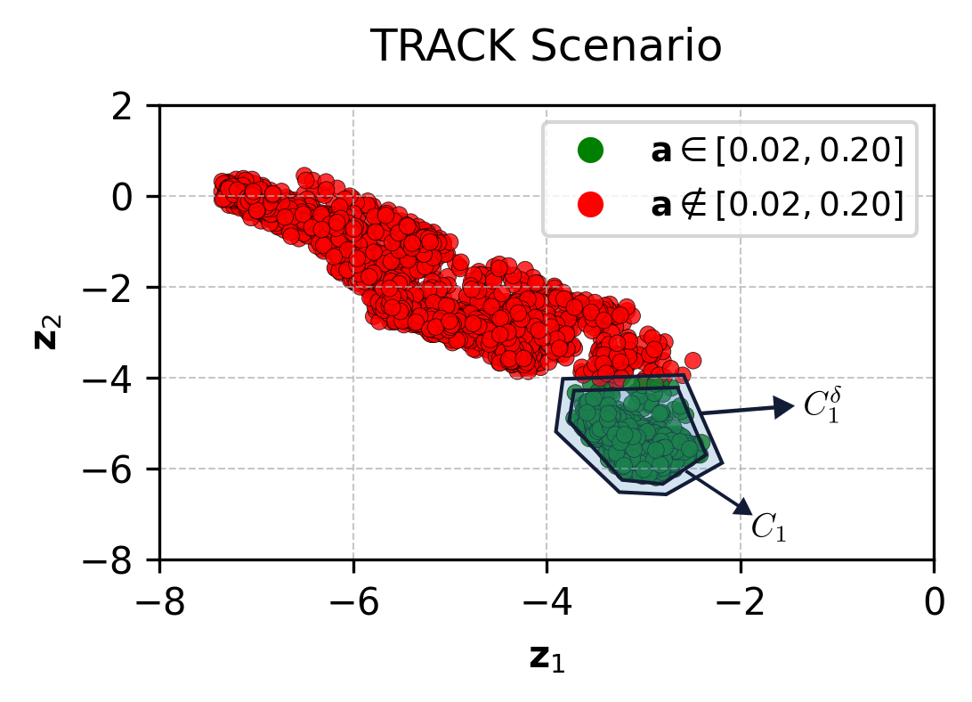
Figure 3. 2D latent space representation of the front camera images from the driving scenario described in Example 3. The variables are labeled by action sets $A_{1}=[0.02,0.20]$ and $A_{2}=A\setminus A_{1}$.

4.4. Formal Verification using Latent Space Convex Polytopes

The convex polytopes $C_{i}$ defined in Section 4.3 facilitates the development of an explainable and scalable framework for verifying image-based neural network controllers. Consider a neural network controller $F(\mathbf{x})$ trained on the same dataset $X$ as the VAE from Section 4.1. Traditional formal verification processes for image-based neural networks involve solving optimization problems as expressed in Equation (4). However, the input space for such problems becomes significantly large, contingent on the dimensionality of the input image $\mathbf{x}\in\mathbb{R}^{h\times w}$. Moreover, the input space subset $X_{i}$ used for verification is limited to a finite and discrete selection of images, which constrains both explainability and scalability.

In contrast, our approach leverages the convex polytope $C_{i}$ to define an explainable and continuous input space in the latent domain. Specifically, $C_{i}$ encompasses a continuous region of latent variables $\mathbf{z}_{i}\in C_{i}$, where each $\mathbf{z}_{i}$ is associated with a control action $\mathbf{a}_{i}\in A_{i}$. This transformation reduces the verification problem’s input space from the high-dimensional $\mathbb{R}^{h\times w}$ to the lower-dimensional latent space $\mathbb{R}^{d_{z}}$.

To perform formal verification of the neural network controller $F(\mathbf{x})$, we first integrate the decoder $D(\mathbf{z})$ with $F(\mathbf{x})$, forming the combined network $\mathcal{H}$ defined as:

$$\mathcal{H}(\mathbf{z})=F(D(\mathbf{z}))$$

For any latent variable $\mathbf{z}$, the combined network $\mathcal{H}(\mathbf{z})$ predicts a control action $\mathbf{a}\in A$. Given that both $F(\mathbf{x})$ and $D(\mathbf{z})$ are neural networks with ReLU activation functions, the composite function $\mathcal{H}(\mathbf{z})$ is piecewise linear and continuous.The proof for the Theorem 4 is provided in the Appendix A.3

Theorem 4.

Given $\mathcal{H}(\mathbf{z})=F(D(\mathbf{z}))$, where both $F$ and $D$ are neural networks employing ReLU activations, and $C_{i}$ is a convex polytope in $\mathbb{R}^{d_{z}}$ defined in Equation (8), finding the local minimum of $F(\mathbf{x})$ over $\mathbf{x}\in D(\mathbf{z})$ is equivalent to finding a local minimum of $\mathcal{H}(\mathbf{z})$ over $\mathbf{z}\in C_{i}$. Formally,

$$\arg\min_{\mathbf{x}\in D(C_{i})}F(\mathbf{x})\ \equiv\ \arg\min_{\mathbf{z}\in C_{i}}\mathcal{H}(\mathbf{z})$$

Consequently, Theorem 4 demonstrates that minimizing $F(\mathbf{x})$ over $\mathbf{x}\in X_{i}$ is equivalent to minimizing $\mathcal{H}(\mathbf{z})$ over $\mathbf{z}\in C_{i}$. Referring to Equations (2) and  (4), the verification process thus for the combined network $\mathcal{H}(\mathbf{z})$ can be formalized as:

$$\mathbf{z}\in C_{i}\implies\mathcal{H}(\mathbf{z})\in A_{i}$$

and the optimization problem to be solved to conduct the verification process can be formalized as:

(10) $$a_{\min}=\min_{\mathbf{z}\in C_{i}}\mathcal{H}(\mathbf{z}),\quad a_{\max}=\max_{\mathbf{z}\in C_{i}}\mathcal{H}(\mathbf{z})$$

subject to $$a_{\min}\in A_{i},\quad a_{\max}\in A_{i},$$

where $C_{i}$ and $A_{i}$ are correlated as described in Lemma 2. It is important to note that the bounds of each action set $A_{i}\subseteq A$ depend on the formal specifications being verified and correspond to a specific convex polytope $C_{i}\subset\mathbb{R}^{d_{z}}$ in the $d_{z}$-dimensional latent space.

4.5. Augmented Latent Spaces for Robustness Verification

In prior sections, we developed the SEVIN framework, which leverages latent representations to formally verify neural network controllers. These representations are derived from the dataset $X$, consisting solely of unperturbed images captured by the front camera of an AV. Consequently, both the reconstructed dataset $\hat{X}$ and the set of convex polytopes $C$ correspond exclusively to clean data. In this section, we will utilize the SEVIN framework to also conduct robustness verification of the neural network controller.

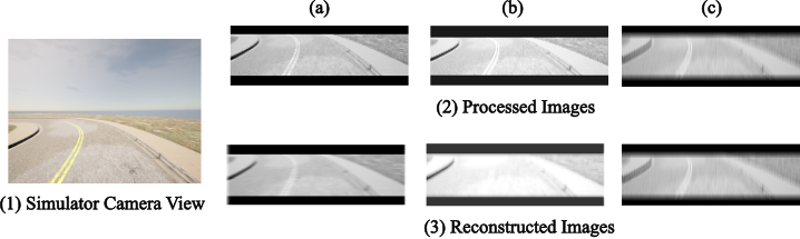
Figure 4. Illustration of the data pre-processing, augmentation, and reconstruction steps used in our approach. (1) Original front camera view captured from the AV within the CARLA driving simulator environment on a two-lane track. (2)(a) Resized and cropped images before training. (b) Augmented image with brightness level adjusted by a random factor $\delta\in[-0.2,0.2]$. (c) Augmented image with motion blur applied, with the degree of blur (kernel size) $\delta\in[1,6]\cap\mathbb{Z}$. (3) Reconstructions of the images from (2) generated by the trained VAE’s.

Figure 4 illustrates some augmentations applied to the dataset of clean images. To verify the robustness of neural network controllers, we construct latent space representations for two datasets, each incorporating a different augmentation type: (1) Image Brightness, (2) Motion Blur, following the SEVIN approach. Each augmentation is quantified and applied to the dataset $X=\{\mathbf{x}\}_{j=1}^{M}$, resulting in an augmented images only dataset $\bar{X}^{\prime}=\bar{\mathbf{x}}_{j=1}^{M}$. The augmented images are then combined with the original dataset to form the new combined augmented and clean dataset, $\bar{X}=X\cup\bar{X}^{\prime}$. From $\bar{X}$, we generate a latent space representation $\bar{Z}$ and the set of convex polytopes $\bar{C}=\bigcup_{i=1}^{I}\bar{C}_{i}$, following the SEVIN formulation outlined in Section 4.3.

Notably, for any action $\mathbf{a}\in A$, $(\bar{\mathbf{x}},\mathbf{a})\in\bar{X}\times A$. This is due the fact that the augmentation is applied only to the image ($\mathbf{x}$) and does not affect the control action ($\mathbf{a}$) to be taken by the controller. Importantly, the augmentations do not alter the action values for any latent variable $\mathbf{z}\in\bar{C}_{i}$, thereby preserving Lemma 1 such that:

$$\forall a\in A,\quad p(\exists\ \bar{\mathbf{z}}\in\bar{Z}\text{ s.t. }(\bar{\mathbf{z}},\mathbf{a})\in\bar{Z}\times A)\ >0$$

In fact, the VAE learns the augmentation applied to the image as an additional feature and can distinguish between the clean and augmented images quite precisely as seen in Figure 5.

Based on the optimization problem corresponding to robustness verification described in (5), we can use the SEVIN framework to formalize the robustness verification process as:

$$\mathbf{z}\in\bar{C}_{i}\implies\mathcal{H}(\mathbf{z})\in A_{i}$$

where the optimization problem to be solved by the neural network verification tool is:

$$a_{\min}=\min_{\mathbf{z}\in\bar{C}_{i}}\mathcal{H}(\mathbf{z}),\quad a_{\max}=\max_{\mathbf{z}\in\bar{C}_{i}}\mathcal{H}(\mathbf{z})$$

subject to $$a_{\min}\in A_{i},\quad a_{\max}\in A_{i}$$

Section 5.3.1 shows the type of augmentations along with the range of values that are applied to the dataset $X$. Individual VAE’s are trained for each augmented dataset $\bar{X}$.

Figure 5. t-SNE plot of an 8D latent space representation generated for the clean ($X$) and motion blur augmented image dataset ($\bar{X}$)

By verifying the neural network controller over $\bar{C}_{i}$, we assess its robustness to input perturbations. SEVIN unifies formal verification and robustness verification within a single framework, leveraging generative AI techniques to scale the verification problem to the continuous domain.

4.6. Designing Symbolic Formal Specifications

The combined network $\mathcal{H}(\mathbf{z})$ undergoes verification against a set of SAFETY and PERFORMANCE specifications within both general formal verification and robustness verification frameworks. These specifications adhere to the Verification of Neural Network Library (VNN-LIB) standard, which is widely recognized for neural network verification benchmarks (Guidotti et al., 2023). The VNN-LIB specification standard builds upon the Open Neural Network Exchange (ONNX) format for model description and the Satisfiability Modulo Theory Library (SMT-LIB) format for property specification, ensuring compatibility and interoperability across various verification tools and platforms. The VNN-LIB standard allows designers to specify bounds on each input and output parameter of the neural network under verification, providing a highly expressive framework for defining verification constraints. The specifications are meticulously crafted to align with the driving scenarios outlined in Section 5.1

SAFETY specifications are designed to guarantee that the neural network controller does not produce unsafe action values within a defined input polytope $C_{i}$. For instance, in natural language, a SAFETY specification for the driving scenario might state that the neural network controller ”always predicts a RIGHT turn if the input image indicates a RIGHT turn”. Formally, this can be expressed as:

$$\varphi_{\text{SAFETY}}\coloneq\ \forall\mathbf{z}\in C_{\text{right}},\{a_{\text{min}},a_{\text{max}}\}\in A_{\text{right}}$$

where $\{a_{\text{min}},a_{\text{max}}\}$ can be calculated by solving the optimization problem from Equation (10). $C_{\text{right}}$ represents the $d_{z}$-dimensional convex polytope in the latent space $Z$ corresponding to images indicative of right turns. The specification denotes for all latent variables $\mathbf{z}$ within $C_{\text{right}}$, the network’s output $\mathcal{H}(\mathbf{z})$ belongs exclusively to the set of steering actions $A_{\text{right}}$ associated with a RIGHT turn.

Conversely, PERFORMANCE specifications aim to ensure that a bounded set of control actions can be achieved from an input convex polytope within the latent space corresponding to the specification. This facilitates the assessment of the neural network controller’s performance across different regions of the input space. The process involves partitioning the entire range of control actions into distinct subsets $A_{i=1}^{I}\subseteq A$. For each action subset $A_{i}$, the corresponding convex polytope $C_{i}$ in the latent space is determined as described in Section 4.3. An exemplary PERFORMANCE specification is presented below:

$$\varphi_{\text{PERFORMANCE}}\coloneq\ \forall\mathbf{z}\in C_{\text{[0.2,0.5]}},\ \{0.2\leq[a_{\text{min}},a_{\text{max}}]\leq 0.5\}$$

where $\{a_{\text{min}},a_{\text{max}}\}$ can be calculated by solving the optimization problem from Equation (10). In this context, $[0.2,0.5]$ delineates the range of steering action values within which the combined network $\mathcal{H}(\mathbf{z})$ is expected to predict a steering value for all $\mathbf{z}\in C_{[0.2,0.5]}$. This formalization ensures that the controller operates within the desired performance bounds across specified input regions.

Table 1. Verification Results for Robust Formal Verification using SEVIN

Augmentation	Specification	Formula	NvidiaNet $\delta_{1}$ = [80-120]%		NvidiaNet $\delta_{2}$ = [60-140]%		ResNet18 $\delta_{1}$ = [80-120]%		ResNet18 $\delta_{2}$ = [60-140]%		ResNet18 $\delta_{3}$ = [50-150]%
			Result	Time(s)	Result	Time(s)	Result	Time(s)	Result	Time(s)	Result	Time(s)
Brightness	Safety	$\varphi_{1}$	SAT	0.412	SAT	0.4027	SAT	0.6189	SAT	0.6293	SAT	0.7109
		$\varphi_{2}$	SAT	0.3739	SAT	0.3637	SAT	0.565	SAT	0.6001	UNSAT	-
	Performance	$\varphi_{1}$	UNSAT	-	UNSAT	-	SAT	0.637	SAT	0.6332	SAT	0.6132
		$\varphi_{2}$	SAT	0.326	SAT	0.39	SAT	0.5933	SAT	0.5588	SAT	0.5860
		$\varphi_{3}$	UNSAT	-	UNSAT	-	SAT	0.853	SAT	0.8011	UNSAT	-
			NvidiaNet $\delta_{1}$ = {1,2}		NvidiaNet $\delta_{2}$ = {3,4}		ResNet18 $\delta_{1}$ = {1,2}		ResNet18 $\delta_{2}$ = {3,4}		ResNet18 $\delta_{3}$ = {5,6}
Motion Blur	Safety	$\varphi_{1}$	SAT	0.304	SAT	0.33	SAT	0.6134	SAT	0.6236	SAT	0.7109
		$\varphi_{2}$	SAT	0.3768	SAT	0.367	SAT	0.629	SAT	0.627	SAT	0.6193
	Performance	$\varphi_{3}$	UNSAT	-	UNSAT	-	SAT	0.616	SAT	0.6477	UNSAT	0.6132
		$\varphi_{4}$	SAT	0.3745	SAT	0.4403	SAT	0.6776	SAT	0.6702	UNSAT	0.5860
		$\varphi_{5}$	SAT	0.5621	UNSAT	-	SAT	0.822	SAT	0.555	UNSAT	-

5. Experiments

To test our proposed approach on an image based neural network controller, we choose an autonomous driving scenario where an AV drives itself around a track in a simulator. One of the goals of our experiments is to test and see if we can generate an explainable latent representation of the image dataset collected by the front camera images. Once we do that, we want to make sure that we can configure the convex polytopes in the latent space as inputs to the verification problem. Finally, we aim to evaluate the controller’s performance by conducting both vanilla formal and robust formal verifications, and compare the performance metrics of our approach to a general image-based neural network robustness verification problem (see more in Section 5.3.5). The VAE’s and neural network controllers are trained on 2x NVIDIA A100 GPU’s and the formal verification is carried out on a NVIDIA RTX 3090 GPU with 24GB of VRAM.

5.1. Driving Scenarios

The driving simulator collects RGB images ($\mathbf{x}$) from the AV’s front-facing camera along with the steering control actions ($\mathbf{a}$). The AV drives on a custom, single-lane track created in RoadRunner by MathWorks and simulated in the CARLA environment. The simulator’s autopilot mode autonomously drives the vehicle, collecting control data, including the steering angle, as the control action ($\mathbf{a}$). The RGB images ($\mathbf{x}$) are resized to 80x64 grayscale images to reduce dimensionality while retaining essential lane information. A snapshot of the front camera view and the processed images used for training can be seen in Figure 4.

We ensure that the camera captures features relevant to the SAFETY and PERFORMANCE properties discussed in Section 4.6. The images are pre-processed to retain only essential lane marking features, which reduces learning redundant features by the VAE, allowing for an easily distinguishable latent space based on differing action sets $A_{i}$.

Table 2. Hyperparameters for VAE Training

Parameter	Value
Latent Dimension	8
Optimizer	Adam
Learning Rate	$1\times 10^{-5}$
Weight Decay	$1\times 10^{-4}$
Epochs	20
$\beta$	0.01

5.2. Network Architectures

The GM-VAE used in our approach consists of an encoder and a decoder network, with convolutional and transposed convolutional layers, respectively, to process and reconstruct data. The encoder progressively increases channel sizes, while the decoder reduces them in reverse order. Each layer integrates batch normalization, ReLU activations, and dropout to prevent overfitting. The encoder begins with a linear layer, followed by three convolutional layers with increasing channel sizes: from 1 to 64, then 128, 256, and finally 512 channels. We employ $K=16$ Gaussians in the mixture model to enhance the expressiveness of the latent representation. A Sigmoid activation function is applied at the output layer to ensure that the generated pixel values are within the range $[0,1]$.

Table 3. Results for Vanilla Formal Verification using SEVIN

Specification		NNC Architecture
		NvidiaNet		ResNet18
		Results	Time(s)	Results	Time(s)
Safety	$\varphi_{1}$	SAT	0.417	SAT	0.6343
	$\varphi_{2}$	SAT	0.4430	SAT	0.7023
Performance	$\varphi_{3}$	SAT	0.412	SAT	0.6799
	$\varphi_{4}$	SAT	0.3667	SAT	0.5746
	$\varphi_{5}$	SAT	0.6383	SAT	0.8215

5.3. Results

We evaluated our proposed method using the neural network verification tool $\alpha-\beta-CROWN$ (Authors, 2023), offering certified bounds on model outputs under specified perturbations. This tool is suitable for verifying the safety and reliability of neural network controllers in autonomous systems. To assess both vanilla formal and robust formal verification methods (Section 4.5), we employed two SAFETY specifications and three PERFORMANCE specifications as described in Section 5.2.

5.3.1. Image Augmentations

For the robust formal verifications, we applied different levels ($\delta_{1,2,3}$) of augmentations to the image dataset to generate $\bar{X}$ for training the VAEs. The types and quantifications of the image augmentations are as follows:

• Brightness: Datasets were generated by randomly varying image brightness levels within specified ranges $\delta_{i}$:

  • $\delta_{1}$: 80% to 120% of original brightness.

  • $\delta_{2}$: 60% to 140% of original brightness.

  • $\delta_{3}$: 50% to 150% of original brightness.

• Vertical Motion Blur: Datasets were generated by varying the degree of vertical motion blur kernels within the ranges:

  • $\delta_{1}$: Kernel sizes of 1 and 2 pixels.

  • $\delta_{2}$: Kernel sizes of 3 and 4 pixels.

  • $\delta_{3}$: Kernel sizes of 5 and 6 pixels.

5.3.2. Specifications

The SAFETY specifications used to verify the controller are defined as:

(11) $$\varphi^{1}_{\text{SAFETY}}\coloneq\forall\mathbf{z}\in C_{[-ve]},\quad\mathcal{H}(\mathbf{z})\leq 0.0,$$

$$\varphi^{2}_{\text{SAFETY}}\coloneq\forall\mathbf{z}\in C_{[+ve]},\quad\mathcal{H}(\mathbf{z})\geq 0.0,$$

where $C_{[-ve]}$ and $C_{[+ve]}$ denote the latent space regions corresponding to negative and positive control actions, respectively.

The PERFORMANCE specifications are defined as:

$$\varphi^{1}_{\text{PERFORM}}\coloneq\forall\mathbf{z}\in C_{[-0.4,-0.1]},\quad-0.4\leq\mathcal{H}(\mathbf{z})\leq-0.1,$$

$$\varphi^{2}_{\text{PERFORM}}\coloneq\forall\mathbf{z}\in C_{[-0.1,0.1]},\quad-0.1\leq\mathcal{H}(\mathbf{z})\leq 0.1,$$

$$\varphi^{3}_{\text{PERFORM}}\coloneq\forall\mathbf{z}\in C_{[0.1,0.4]},\quad 0.1\leq\mathcal{H}(\mathbf{z})\leq 0.4,$$

where $C_{[a,b]}$ represents the latent space regions corresponding to control actions between $a$ and $b$.

These specifications were used for both vanilla formal and robust formal verification methods. The verification results, along with the input formal specifications, applied image augmentations, and evaluated neural network controllers, are summarized in Table 3 and Table 1.

5.3.3. Vanilla Formal Verification:

From the results, we can infer that both the vanilla and robust formal verification processes take ¡ 1 second to conduct verification. This is due to the reduction in computational complexity of the processes as we introduce lower dimensional input spaces in the form of convex polytopes ($C$). Additionally, we also note that for the vanilla formal verification, the neural network controllers satisfy all of the specifications provided. This indicates that the controllers provide formal guarantees with respect to both the SAFETY and PERFORMANCE specifications when the input space $C_{i}$ belongs to clean image sets $X_{i}$.

5.3.4. Robust Formal Verification:

For the robust formal verification process, we can notice specifications $\varphi_{3}$ and $\varphi_{5}$ to be unsatisfactory for the NvidiaNet architecture, for both levels and types of augmentations, $\delta_{1}$ and $\delta_{2}$. The NvidiaNet architecture thus seems to be more susceptible to image augmentations and fairs poorly during the robustness verification process. In contrast, the ResNet18 architecture tends to perform fairly better than NvidiaNet for the $\delta_{1}$ and $\delta_{2}$ levels of augmentations for both vertical motion blur and brightness variation. It starts providing unsatisfactory verification results once the $\delta_{3}$ level of augmentations are applied to both types of image augmentations. This shows that the ResNet18 architecture is more robust than NvidiaNet in handling image perturbations for the case of autonomous driving scenarios.

5.3.5. Scalability Comparison:

We conduct general robustness verification on the neural network controller $F(\mathbf{x})$ using the $\alpha-\beta-CROWN$ toolbox and compare these results with those obtained via the SEVIN framework. We employ the same set of SAFETY specifications as described in Equation (11), and we separate the brightness-augmented dataset $\bar{X}$ into two subsets, $\bar{X}_{[-\text{ve}]}$ and $\bar{X}_{[+\text{ve}]}$, based on their corresponding negative and positive control action sets, $A_{[-\text{ve}]}$ and $A_{[+\text{ve}]}$. By converting $F(\mathbf{x})$ into the ONNX format and defining perturbation bounds for each dimension (i.e., pixel) of $\mathbf{x}$, we leverage the neural network verification tool to perform robustness verification directly on the original high-dimensional image inputs. The upper and lower bounds are calculated for all images $\mathbf{x}\in\bar{X}_{[-\text{ve}]}$ and $\mathbf{x}\in\bar{X}_{[+\text{ve}]}$. The results are shown in Table 4.
When comparing the results between Table 1 and 4, we observe that all the specifications are SAT for both methods. However, a significant difference lies in the time taken by the general method, which is almost ten times longer than that of the SEVIN method. This substantial difference is due to the fact that the input dimensionality of the verification problem using the SEVIN framework is approximately 600 times smaller than that of the general framework, making the problem computationally less complex and, consequently, more scalable to larger networks. Although for SEVIN, the combined network ($\mathcal{H}$) to be verified has many more layers than the neural network controller ($F$).

Table 4. Results for General Robust Formal Verification using the Neural Network Verification toolbox

Augmentation	Specification		NNC Architecture
			NvidiaNet		ResNet18
			Results	Time(s)	Results	Time(s)
Brightness	Safety	$\varphi_{1}$	SAT	3.213	SAT	4.257
		$\varphi_{2}$	SAT	4.165	SAT	4.958

6. Conclusion

We provide a framework for scalable and explainable formal verification of image based neural network controllers (SEVIN). Our approach involves developing a trained latent space representation for the image dataset used by the neural network controller. By using control action values as labels, we classify the latent variables and generate convex polytopes as input spaces for the verification process. We concatenate the decoder network of the Variational Autoencoder (VAE) with the neural network controller, allowing us to directly map lower-dimensional latent variables to higher-dimensional control action values.Once the verification input space is made explainable, we construct specifications using symbolic languages such as Linear Temporal Logic (LTL). We then provide the neural network verification tool with the combined network and the specifications for verification. To enhance the formal robustness verification process, we generate an augmented dataset and retrain the VAEs to produce new latent representations.Finally, we test the SEVIN framework on two neural network controllers in an autonomous driving scenario, using two sets of specifications—SAFETY and PERFORMANCE—for both the standard formal verification and robustness verification processes. In the future, we aim to conduct reachability analysis using the SEVIN framework for neural network controllers with their specified plant model.

Appendix A Proofs for Lemmas and Theorems

A.1. Proof of Lemma 1

Proof.

For each action value $\mathbf{a}\in A$, there exists at least one image $\mathbf{x}\in X$ such that the associated control action is $\mathbf{a}$. By applying the encoder to any such image $\mathbf{x}$, we obtain the latent variable $\mathbf{z}=E(\mathbf{x})$. Thus, the pair $(\mathbf{z},\mathbf{a})$ exists in $Z\times A$.

Since the latent variables $\mathbf{z}$ are generated from images $\mathbf{x}$ via the encoder $E(\mathbf{x})$, and the latent space $Z$ follows the GM prior $p(\mathbf{z})$, this prior $p(\mathbf{z})$ serves as the probability density function over $Z$. Therefore, $p(\mathbf{z})$ assigns a positive probability to all latent variables in $Z$ that correspond to images in $X$ under the mapping $E(\mathbf{x})$.

Formally, for any $\mathbf{a}\in A$, we define the set of latent variables corresponding to $\mathbf{a}$ as:

(12) $$Z_{\mathbf{a}}=\left\{\mathbf{z}\in Z|\exists\mathbf{x}\in X\ \text{s.t.}\ \mathbf{a}=F(\mathbf{x})\text{ and }\mathbf{z}=E(\mathbf{x})\right\}$$

Since $Z_{\mathbf{a}}$ is non-empty and $p(\mathbf{z})$ is a valid probability density function over $Z$, it follows that:

(13) $$p\left(\mathbf{z}\in Z_{\mathbf{a}}\right)=\int_{Z_{\mathbf{a}}}p(\mathbf{z})\,d\mathbf{z}>0$$

Thus, there exists a positive probability of sampling a latent variable $\mathbf{z}$ corresponding to any action $\mathbf{a}\in A$, establishing the result stated in Equation (7). ∎

A.2. Proof of Lemma 2

Proof.

By construction, the convex polytope $C_{i}\subset\mathbb{R}^{d_{z}}$ is formed from $n$ latent samples $\{\mathbf{z}_{j}\}_{j=1}^{n}$ drawn from the GM prior $p(\mathbf{z})$ within two standard deviations from the mean $\boldsymbol{\mu}_{A_{i}}$ corresponding to the action set $A_{i}$. Specifically, each sampled latent variable $\mathbf{z}_{j}$ satisfies:

$$\|\mathbf{z}_{j}-\boldsymbol{\mu}_{A_{i}}\|_{2}\leq 2\sigma_{A_{i}}$$

Since $C_{i}$ is the convex hull of these samples, any $\mathbf{z}\in C_{i}$ can be expressed as a linear combination of the sampled latent variables:

$$\mathbf{z}=\sum_{j=1}^{n}\lambda_{j}\mathbf{z}_{j},\quad\text{where }\lambda_{j}\geq 0\text{ and }\sum_{j=1}^{n}\lambda_{j}=1$$

The decoder $D(\mathbf{z})$ is assumed to be a continuous function mapping latent variables to high-dimensional images. Therefore, decoding $\mathbf{z}\in C_{i}$ yields:

$$\hat{\mathbf{x}}=D(\mathbf{z})=D\left(\sum_{j=1}^{n}\lambda_{j}\mathbf{z}_{j}\right)$$

Specifically, since each latent variable $\mathbf{z}_{j}$ corresponds to an action $\mathbf{a}_{j}\in A_{i}$, and $A_{i}$ is a continuous action set, the convex combination ensures that $\hat{\mathbf{x}}$ is associated with an action $\mathbf{a}\in A_{i}$.

Formally, for each $\mathbf{z}\in C_{i}$, there exists an image $\hat{\mathbf{x}}\in\mathbb{R}^{h\times w}$ such that:

$$(\hat{\mathbf{x}},\mathbf{a})^{i}\in\mathbb{R}^{h\times w}\times A_{i}$$

This establishes that decoding any latent variable within the convex polytope $C_{i}$ produces an image associated with the action set $A_{i}$.

Consequently, the convex polytope $C_{i}$ effectively encapsulates a continuous region in the latent space corresponding to the action set $A_{i}$, ensuring that all decoded images $\hat{\mathbf{x}}$ from $C_{i}$ are correctly paired with actions $\mathbf{a}\in A_{i}$. ∎

A.3. Proof of Theorem 1

Proof.

By Lemma 1, for each action $\mathbf{a}\in A$, there exists a latent variable $\mathbf{z}\in Z$ such that the pair $(\mathbf{z},\mathbf{a})$ is in $Z\times A$ with positive probability under the prior $p(\mathbf{z})$. This ensures that the latent space $Z$ is meaningfully connected to the action space $A$, and the mapping between images and actions is preserved in the latent space.

According to Lemma 2, any latent variable $\mathbf{z}\in C_{i}$ can be decoded using $D(\mathbf{z})$ to generate a reconstructed image $\hat{\mathbf{x}}$. This image forms a pair $(\hat{\mathbf{x}},\mathbf{a})^{i}$ with an action $\mathbf{a}\in A_{i}$, indicating that the decoder $D$ maps the convex polytope $C_{i}$ in latent space back to meaningful images in the original space $X$.

Neural networks with ReLU activations, such as $F$ and $D$, are known to be piecewise linear functions (Montufar et al., 2014; Raghu et al., 2017). They partition their input spaces into polyhedral regions within which the functions act linearly. The composition $\mathcal{H}(\mathbf{z})=F(D(\mathbf{z}))$ thus inherits this piecewise linearity because the composition of piecewise linear functions is also piecewise linear (Bronstein et al., 2017).

From the properties established in Lemma 2, $D$ maps the convex polytope $C_{i}$ in latent space to a corresponding polyhedral region in the image space $X$. This means that optimizing $F(\mathbf{x})$ over $\mathbf{x}\in D(C_{i})$ is equivalent to optimizing $\mathcal{H}(\mathbf{z})$ over $\mathbf{z}\in C_{i}$, since $D$ provides a bijective linear mapping within these regions.

Moreover, since a local minimum of a piecewise linear function occurs at a vertex or along an edge of its polyhedral regions (Clarke, 1998), the local minima of $\mathcal{H}(\mathbf{z})$ over $\mathbf{z}\in C_{i}$ correspond directly to the local minima of $F(\mathbf{x})$ over $\mathbf{x}\in D(C_{i})$. Therefore, optimizing $F(\mathbf{x})$ over the high-dimensional space $X_{i}$ is equivalent to optimizing $\mathcal{H}(\mathbf{z})$ over the lower-dimensional latent space polytope $C_{i}$, establishing the equivalence of the two optimization problems (Kawaguchi, 2016; Choromanska et al., 2015).

∎

References

- (1)
- Akazaki and Liu (2018) Takumi Akazaki and Yang Liu. 2018. Falsification of Cyber-Physical Systems Using Deep Reinforcement Learning. In International Symposium on Formal Methods. Springer, 456–465.
- Authors (2023) Alpha Beta CROWN Authors. 2023. Alpha-beta-CROWN: Scalable Neural Network Verification with Optimized Bound Propagation. arXiv preprint arXiv:AlphaBetaCROWN (2023).
- Barber et al. (1996) C Bradford Barber, David P Dobkin, and Hannu Huhdanpaa. 1996. The Quickhull Algorithm for Convex Hulls. ACM Transactions on Mathematical Software (TOMS) (1996).
- Bronstein et al. (2017) Michael M Bronstein, Joan Bruna, Yann LeCun, Arthur Szlam, and Pierre Vandergheynst. 2017. Geometric Deep Learning: Going Beyond Euclidean Data. IEEE Signal Processing Magazine (2017).
- Bunel et al. (2018) Rudy Bunel, Isil Dillig Turkaslan, and Philip HS Torr. 2018. A Unified View of Piecewise Linear Neural Network Verification. Advances in Neural Information Processing Systems (2018).
- Choromanska et al. (2015) Anna Choromanska, Mikael Henaff, Michael Mathieu, Gerard Ben Arous, and Yann LeCun. 2015. The Loss Surfaces of Multilayer Networks. Proceedings of the Eighteenth International Conference on Artificial Intelligence and Statistics (2015).
- Clarke (1998) Frank H Clarke. 1998. Nonsmooth Analysis and Control Theory. Springer.
- Dilokthanakul et al. (2016) Nat Dilokthanakul, Pedro AM Mediano, Marta Garnelo, Matthew CH Lee, Hugh Salimbeni, Kai Arulkumaran, and Murray Shanahan. 2016. Deep Unsupervised Clustering with Gaussian Mixture Variational Autoencoders. arXiv preprint arXiv:1611.02648 (2016).
- Ehlers (2017) Rüdiger Ehlers. 2017. Formal Verification of Piecewise Linear Feed-Forward Neural Networks. arXiv preprint arXiv:1705.01320 (2017).
- Gehr et al. (2018) Timon Gehr, Matthew Mirman, Dana Drachsler-Cohen, Petar Tsankov, and Martin Vechev. 2018. AI2: Safety and Robustness Certification of Neural Networks with Abstract Interpretation. 2018 IEEE Symposium on Security and Privacy (SP) (2018).
- Grünbaum (2003) Branko Grünbaum. 2003. Convex Polytopes. Vol. 221. Springer Science & Business Media.
- Guidotti et al. (2023) Dario Guidotti, Stefano Demarchi, Armando Tacchella, and Luca Pulina. 2023. The Verification of Neural Networks Library (VNN-LIB). https://www.vnnlib.org Accessed: 2023.
- Higgins et al. (2017) Irina Higgins, Loic Matthey, Arka Pal, Christopher Burgess, Alexander Glorot-Xavier, and Matthew Botvinick. 2017. beta-VAE: Learning Basic Visual Concepts with a Constrained Variational Framework. International Conference on Learning Representations (2017).
- Huang et al. (2017) Xiaowei Huang, Marta Kwiatkowska, Sen Wang, and Min Wu. 2017. Safety Verification of Deep Neural Networks. arXiv preprint arXiv:1610.06940 (2017).
- Kaiser et al. (2021) Eli Kaiser, Saif Ahmed, and Tommaso Dreossi. 2021. SMT-Based Verification of Neural Network Controllers for Autonomous Systems. IEEE Transactions on Cybernetics (2021).
- Katz et al. (2017a) Guy Katz, Clark Barrett, David L Dill, Kyle Julian, and Mykel J Kochenderfer. 2017a. Reluplex: An Efficient SMT Solver for Verifying Deep Neural Networks. arXiv preprint arXiv:1702.01135 (2017).
- Katz et al. (2017b) Guy Katz, Clark Barrett, David L Dill, Kyle Julian, and Mykel J Kochenderfer. 2017b. Towards Scalable Verification for All Neural Networks. arXiv preprint arXiv:1702.01135 (2017).
- Kawaguchi (2016) Kenji Kawaguchi. 2016. Deep Learning without Poor Local Minima. arXiv preprint arXiv:1605.07110 (2016).
- Kingma and Welling (2013) Diederik P Kingma and Max Welling. 2013. Auto-Encoding Variational Bayes. arXiv preprint arXiv:1312.6114 (2013).
- Liu et al. (2019) Changliu Liu, Tamar Arnon, Christopher Lazarus, Alexander Strong, Clark Barrett, and Mykel J Kochenderfer. 2019. Algorithms for Verifying Neural Networks. arXiv preprint arXiv:1903.06758 (2019).
- Montufar et al. (2014) Guido F Montufar, Razvan Pascanu, Kyunghyun Cho, and Yoshua Bengio. 2014. On the Number of Linear Regions of Deep Neural Networks. arXiv preprint arXiv:1402.1869 (2014).
- Pnueli (1977) Amir Pnueli. 1977. The Temporal Logic of Programs. 18th Annual Symposium on Foundations of Computer Science (sfcs 1977) (1977).
- Raghu et al. (2017) Maithra Raghu, Ben Poole, Jon Kleinberg, Surya Ganguli, and Jascha Sohl-Dickstein. 2017. On the Expressive Power of Neural Networks with Relu Activations. arXiv preprint arXiv:1711.02060 (2017).
- Rezende et al. (2014) Danilo Jimenez Rezende, Shakir Mohamed, and Daan Wierstra. 2014. Stochastic Backpropagation and Approximate Inference in Deep Generative Models. (2014).
- Ruan et al. (2018) Wenjie Ruan, Xinming Huang, and Marta Kwiatkowska. 2018. Reachability Analysis of Deep Neural Networks with Provable Guarantees. arXiv preprint arXiv:1805.02242 (2018).
- Schneider (1993) Rolf Schneider. 1993. Convex Bodies: The Brunn-Minkowski Theory. Cambridge University Press (1993).
- Singh et al. (2018) Gagandeep Singh, Timon Gehr, Markus Püschel, and Martin Vechev. 2018. Fast and Effective Robustness Certification. Advances in Neural Information Processing Systems (2018).
- Singh et al. (2019) Gagandeep Singh, Timon Gehr, Markus Püschel, and Martin Vechev. 2019. An Abstraction-Based Framework for Neural Network Verification. arXiv preprint arXiv:1810.09031 (2019).
- Tjeng et al. (2019) Vincent Tjeng, Kai Xiao, and Russ Tedrake. 2019. Evaluating Robustness of Neural Networks with Mixed Integer Programming. arXiv preprint arXiv:1711.07356 (2019).
- Tomczak and Welling (2018) Jakub M Tomczak and Max Welling. 2018. VAE with a VampPrior. Proceedings of the 21st International Conference on Artificial Intelligence and Statistics (2018).
- van der Maaten and Hinton (2008) Laurens van der Maaten and Geoffrey Hinton. 2008. Visualizing Data using t-SNE. Journal of Machine Learning Research (2008).
- Vasilache et al. (2022) Andrei Vasilache, Lucas Brodbeck, and Tommaso Dreossi. 2022. Verifying Temporal Logic Specifications in Neural Network Controllers. 2022 ACM/IEEE 6th International Conference on Formal Methods in Software Engineering (FormaliSE) (2022).