Asymmetrical Latent Representation for Individual Treatment Effect Modeling

Abstract

Conditional Average Treatment Effect (CATE) estimation, at the heart of counterfactual reasoning, is a crucial challenge for causal modeling both theoretically and applicatively, in domains such as healthcare, sociology, or advertising. Borrowing domain adaptation principles, a popular design maps the sample representation to a latent space that balances control and treated populations while enabling the prediction of the potential outcomes. This paper presents a new CATE estimation approach based on the asymmetrical search for two latent spaces called Asymmetrical Latent Representation for Individual Treatment Effect (Alrite), where the two latent spaces are respectively intended to optimize the counterfactual prediction accuracy on the control and the treated samples. Under moderate assumptions, Alrite admits an upper bound on the precision of the estimation of heterogeneous effects (PEHE), and the approach is empirically successfully validated compared to the state of the art.

Keywords : Causal inference, Representation learning

1 Introduction

In the Neyman-Rubin framework Rubin, (2005), causal inference focuses on a simple question: how different would the outcome have been if the treatment had been different? Answering this question, however, raises considerable difficulties, as the true answer is inevitably unknown: the $i$-th individual either is treated (with outcome $y_{i}^{1}$) or not (with outcome $y_{i}^{0}$). In both cases, observation of the difference $y_{i}^{1}-y_{i}^{0}$ remains inaccessible. Overall, the estimation of the individual causal effect, acknowledged as the fundamental problem of causal inference (Holland,, 1986), addresses a machine learning problem with missing values.

A most natural approach consists in independently modeling outcome $Y^{1}$ (respectively $Y^{0}$) from the treated (resp. untreated, or control) samples as functions of their covariate description $X$, allowing the individual causal effect to be estimated from the difference of both models. This approach is valid subject to a key assumption, stating that treated and control samples are drawn from the same distribution $\mathbb{P}(X)$; in other words, the treatment assignment must follow the randomized control trial methodology.

In real-life applications however, this assumption rarely holds true. In the medical field the treatment variable $T$ is generally assigned by the doctor, depending on the severity of the individual’s condition. In the field of education, the decision of e.g. following a curriculum depends on the individual’s background. In such cases, the treated and control distributions $\mathbb{P}_{1}(X)=P(X|T=1)$ and $\mathbb{P}_{0}(X)=\mathbb{P}(X|T=0)$ are different.

Estimating the potential outcome models based on the joint distributions $\mathbb{P}(X,Y^{1})$ and $\mathbb{P}(X,Y^{0})$ can thus be cast as a learning across domain problem (Ben-David et al.,, 2006; Ganin et al.,, 2016), where the two support distributions $P(X|T=0)$ and $P(X|T=1)$ differ. Building upon the state of the art (Ben-David et al.,, 2006), it thus comes naturally to integrate the space of original covariates into a latent space aligning both support distributions (Johansson et al.,, 2016; Shalit et al.,, 2017) (more in Section 2).

A main claim of the paper is that the CATE problem however significantly differs from the mainstream learning across domain setting. Specifically, estimating $\mathbb{P}(Y^{1}|X).\mathbb{P}_{0}(X)$ from $\mathbb{P}(Y^{1}|X).\mathbb{P}_{1}(X)$ requires all control samples to be ‘sufficiently close’ from some treated samples (A). Likewise, estimating $\mathbb{P}(Y^{0}|X).\mathbb{P}_{1}(X)$ from $\mathbb{P}(Y^{0}|X).\mathbb{P}_{0}(X)$ requires all treated samples to be ‘sufficiently close’ from some control samples (B). The difference between these requirements is illustrated on Fig. 1: the leftmost and rightmost images correspond to criteria (A) and (B) respectively, while the center image corresponds to a representation suitable for learning across domains.

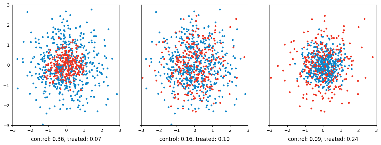
Figure 1: Average counter-factualizability (definition in section 3.2.1) for treated and control samples in latent space. Left: the distributions support a good counter-factual estimation for treated samples (but less so for control samples). Middle: the distributions support a decent ounter-factual estimation for both populations. Right: the distributions support a good counter-factual estimation for control samples (but less so for treated samples).

The main contribution of the present paper is to formalize the intuition that CATE estimation involves two intertwined learning across domain problems, appealing to different requirements. The presented analysis motivates the design of an original model architecture, called Asymmetrical Latent Representation for Individual Treatment Effect (Alrite), as well as new learning criteria, offering formal guarantees on the quality of the learned CATE estimate.

This article is organized as follows. After presenting the formal background, Section 2 briefly introduces and discusses related work. Section 3 gives an overview of the proposed Alrite, and presents its formal analysis. Section 4 presents a comprehensive comparative empirical evaluation of the approach, and the paper concludes with some research perspectives.

Notations.

The observation dataset is noted $\mathcal{D}=\{(x_{i},t_{i},y_{i}),i=1\ldots n\}$, where $x_{i}\in\mathcal{X}\subset\mathbb{R}^{d}$, $t_{i}\in\{0,1\}$ and $y_{i}\in\mathcal{Y}\subset\mathbb{R}$ respectively denote the covariate, the treatment assignment and the observed outcome for the $i$-th sample, with $t_{i}=1$ (respectively $t_{i}=0$) for a treated (resp. control) sample; $n_{0}$ and $n_{1}$ respectively denote the number of control and treated samples. As usual, upper case letters denote random variables in the following, while lower case ones refer to observations.

Assumptions.

Alrite is based on the three standard assumptions for counterfactual estimation (Rubin,, 1978; Rosenbaum and Rubin,, 1983) within the Neyman-Rubin framework (Rubin,, 2005): conditional exchangeability, positivity,, and Stable Unit Treatment Value Assumption (SUTVA):

• $\forall t\in\{0,1\},\ Y^{t}\perp\!\!\!\perp T\ |\ X$

• $\forall\ A\subset\mathcal{X}\ ,\ \mathbb{P}(X\in A)>0\ \implies\mathbb{P}(X\in A|T=1),\mathbb{P}(X\in A|T=0)>0$

• $Y=(1-T)\,Y^{0}+T\,Y^{1}$

Quantity of interest and performance metrics.

The Conditional Average Treatment Effect (CATE, denoted by $\tau$) is an estimate of the expected impact of the treatment at the subpopulation/individual level:

$$\tau:x\mapsto\mathbb{E}[Y^{1}-Y^{0}|X=x]$$

The performance of the CATE estimate is usually assessed using the Precision in Estimation of Heterogeneous Effect (PEHE) when the ground truth $\tau$ is available, and either the Policy Risk ($\textit{R}_{\textit{pol}}$) or the Observational Policy Risk ($\textit{oR}_{\textit{pol}}$) otherwise, with:

$$\textit{PEHE}:\hat{\tau}\mapsto \ \mathbb{E}\big{[}(\tau(X)-\hat{\tau}(X))^{2}\big{]}$$

$$\mbox{$\textit{R}_{\textit{pol}}$}:\hat{\tau}\mapsto \ 1-\mathbb{P}(\hat{\tau}(X)>0)\mathbb{E}[Y^{1}|\hat{\tau}(X)>0] -\mathbb{P}(\hat{\tau}(X)\leq 0)\mathbb{E}[Y^{0}|\hat{\tau}(X)\leq 0]$$

$$\mbox{$\textit{oR}_{\textit{pol}}$}:\hat{\tau}\mapsto \ 1-\mathbb{P}(\hat{\tau}(X)>0)\mathbb{E}[Y|\hat{\tau}(X)>0,T=1] -\mathbb{P}(\hat{\tau}(X)\leq 0)\mathbb{E}[Y|\hat{\tau}(X)\leq 0,T=0]$$ (1)

Note that if the treatment assignment is uniform, then $\textit{R}_{\textit{pol}}$ and $\textit{oR}_{\textit{pol}}$ coincide. For the sake of readability and when no confusion is to fear the empirical counterparts of the above expectations are still denoted PEHE, $\textit{R}_{\textit{pol}}$ and $\textit{oR}_{\textit{pol}}$.

2 State of the art

As large datasets become increasingle available, they support the estimation of causal effects at individual or group level, reflecting the heterogeneity of treatment impacts. The state of the art commonly distinguishes several categories of CATE learners, depending on the main features of the models and notably how these models account for the treatment assignment variable Künzel et al., (2019); Nie and Wager, (2021); Kennedy, (2023).

2.1 S-learners 

S(ingle)-learners fit a single model with treatment assignment $T$ and covariates $X$ as inputs. The potential outcome models are learned along classical supervised learning, with:

$$\mbox{$\hat{\mu}$}(x,t)\approx\mu^{t}(x)=\mathbb{E}[Y|X=x,T=t]$$

and the treatment effect is defined as: $\hat{\tau}(x)=\mbox{$\hat{\mu}$}(x,1)-\mbox{$\hat{\mu}$}(x,0)$. In the Balancing Neural Network (BNN) approach Johansson et al., (2016), an embedding $\phi$ is used to map the covariate space onto a latent representation, merging the (image of) control and treatment distributions along the domain adaptation principles (Ben-David et al.,, 2006). The potential outcome $\mbox{$\hat{\mu}$}(x,t)$ is sought as a single neural net, operating on the concatenation of $\phi(x)$ and the treatment variable $t$. However, the fact that the treatment assignment variable is given no particular role tends to bias the CATE estimate toward 0 according to Künzel et al., (2019).

Bayesian Additive Regression Trees (BART) are built along the same principles, using regression trees instead of neural nets; in Athey and Imbens, (2016), the BART approach is extending to yield confidence intervals. In Wager and Athey, (2018), BART is learned using Causal Forests (CF) where the last split of the forest trees corresponds to the treatment assignment.

2.2 T-learners 

T(wo)-learners differ from S-learners in that they learn different models for both potential outcomes. Inspired by domain adaptation Johansson et al., (2022), Shalit et al., (2017) define a single latent space for both control and treated samples (more in Caron et al., (2022)). On this latent space, two independent functions are learned to estimate the potential outcomes:

$$\mbox{$\hat{\mu}$}^{0}(x)\approx\mu^{0}(x)=\mathbb{E}[Y|X=x,T=0]$$

$$\mbox{$\hat{\mu}$}^{1}(x)\approx\mu^{1}(x)=\mathbb{E}[Y|X=x,T=1]$$

with the individual treatment effect being likewise defined as their difference ($\hat{\tau}_{T}(x)=\mbox{$\hat{\mu}$}^{1}(x)-\mbox{$\hat{\mu}$}^{0}(x)$). In Shalit et al., (2017), the BNN S-learner is extended to the T-learner setting. The embedding $\phi$ is trained to minimize the Wasserstein distance (Cuturi,, 2013) or the Maximum Mean Discrepancy (Gretton et al.,, 2012) between the image of the control and treatment distributions. The impact thereof is inspected by contrasting CFR (constrained distance) and TARNet (unconstrained). Other approaches aim to preserve local similarity information in the latent space, such as SITE Yao et al., (2018) or ACE (Yao et al.,, 2019). CFR-ISW (Hassanpour and Greiner, 2019a, ) and BWCFR Assaad et al., (2021) use context-aware weights, reweighting samples in the latent space according to their estimated propensity scores. MitNet (Guo et al.,, 2023) differs from CFR by relying on the mutual information between control and treatment distribution, with the advantage that it handles non-binary treatment settings. StableCFR (Wu et al., 2023a, ) bridges the gap between T-learners and matching methods (Stuart,, 2010): minority distribution is up-sampled using nearest-neighbor approaches in latent space.

Taking inspiration from adversarial domain adaptation (Ganin et al.,, 2016), ABCEI (Du et al.,, 2021) leverages the mutual information between the observed and the latent representation to limit the loss of information; CBRE (Zhou et al.,, 2021) considers an auto-encoder architecture with a specific cycle structure: the loss of information due to the latent representation is prevented by requiring this latent information to support the reconstruction of the samples.

Generative models are also leveraged for CATE. CEVAE (Louizos et al.,, 2017) combines the approach in Shalit et al., (2017) with a Variational Auto-Encoder (VAE) (Kingma and Welling,, 2014; Rezende et al.,, 2014); GANITE (Yoon et al.,, 2018) is based on Generative Adversarial Networks (GAN) (Goodfellow et al.,, 2014). NSGP (Alaa and Schaar,, 2018) and DKLITE Zhang et al., (2020) are based on Gaussian processes, enabling to minimize counter-factual variance and to provide uncertainty intervals.

Refined neural architectures distinguish confounding variables (covariates that cause both $T$ and $Y^{0},Y^{1}$), and adjustment variables (causes of $Y^{0},Y^{1}$ only), in a linear ($\textbf{D}^{2}\textbf{VD}$ (Kuang et al.,, 2017)) or non-linear setting ($\textbf{N-D}^{2}\textbf{VD}$ (Kuang et al.,, 2022)). DR-CFR (Hassanpour and Greiner, 2019b, ) improves on such refined architectures, by introducing one latent representation for instrumental variables (causes of $T$ only), one for confounding variables, and one for adjustment variables. The latent space is trained in various ways: by minimizing the MMD between the latent adjustment representation of control and treated samples (Hassanpour and Greiner, 2019b, ), by leveraging Contrastive Log-Ratio Upper Bound (Cheng et al.,, 2020) in MIM-DRCFR (Cheng et al.,, 2022); by using a deep orthogonal regularizer in DeR-CFR (Wu et al., 2023b, ); by enforcing the disentanglement using adversarial learning Chauhan et al., (2023). The latent structure is combined with a variational approach in TEDVAE (Zhang et al.,, 2021); it is yet further refined in SNet (Curth and Schaar,, 2021), distinguishing adjustment factors causing $Y^{0}$ only, $Y^{1}$ only, and both of them.

2.3 Other approaches

X-learners Künzel et al., (2019); Stadie et al., (2018); Curth and Schaar, (2021) involve a two-step process. In the first step, models of the response functions $\mbox{$\hat{\mu}$}^{0},\mbox{$\hat{\mu}$}^{1}$ and propensity $\hat{\eta}$ are learned. In the second step, two CATE estimates are trained: $\hat{\tau}^{1}(x_{i})\approx y_{i}^{1}-\mu^{0}(x_{i})$ is optimized on treated samples, while $\hat{\tau}^{0}(x_{i})\approx\mu^{1}(x_{i})-y_{i}^{0}$ is optimized on control ones. Finally, the CATE estimate for any given sample is obtained as

$$\hat{\tau}_{X}(x)=(1-\mbox{$\hat{\eta}$}(x))\hat{\tau}_{0}(x)+\mbox{$\hat{\eta}$}(x)\hat{\tau}_{1}(x)$$

R(obinson)-learners Nie and Wager, (2021) extend the CATE typology defined by Künzel et al., (2019), building upon the Robinson’s potential outcome formalization (Robinson,, 1988):

$$Y-\mathbb{E}[Y|X]=(T-\mathbb{E}[T|X])\tau(X)+\varepsilon$$ (2)

with $\varepsilon$ a centered noise variable. Like X-learners, R-learners proceed along a two-stage approach: they first learn $\hat{m}(x)\approx\mathbb{E}[Y|X=x]$ and $\mbox{$\hat{\eta}$}(x)\approx\mathbb{E}[T|X=x]$, and in a second stage the CATE estimate $\hat{\tau}_{R}$ is learned by minimizing:

$$\sum_{i}\big{(}y_{i}-\hat{m}(x_{i})-(t_{i}-\mbox{$\hat{\eta}$}(x_{i}))\hat{\tau}_{R}(x_{i})\big{)}^{2}$$

Using cross-fitting training procedures, this method provably achieves an optimal convergence rate, i.e., as if the true $\eta$ and $m$ were known.

Related approaches include F-learners (Künzel et al.,, 2019) and U-learners (Signorovitch,, 2007; Athey and Imbens,, 2016; Curth and Schaar,, 2021) using other decompositions of the potential outcome models: DR-learners Foster and Syrgkanis, (2023); Kennedy, (2023) introduce a double robustness methodology (Chernozhukov et al.,, 2017); B-learners (Oprescu et al.,, 2023) generalize them in settings with a limited amount of unobserved confounders; and IF-learners (Curth et al., 2021a, ) leverage efficient influence functions (Hampel et al.,, 1986) to enforce double robustness.

2.4 Discussion

The state of the art shows the value of a change of representation for tackling CATE; X-learners, unable to align the control and processing distributions, are at a disadvantage.

The search for a latent space faces two difficulties. On one hand, there is no consensus about how to align both distributions (using ad hoc penalization terms (Johansson et al.,, 2016), MMD Shalit et al., (2017), Wasserstein distance, adversarial learning Du et al., (2021)). On the other hand, the latent space is meant to enforce this alignment for both potential outcome models, and must thus achieve some trade-off between both.

Lastly, Zhang et al., (2020) suggests that the latent space should yield a low counter-factual variance (as opposed to, aligning the control and treated distributions). Formally, high variance on the counter-factual posterior distribution suggests that there is not enough information in the considered region regarding the counter-factual modeling task. How to evaluate the counter-factual variance outside of the Bayesian framework, however, remains an open question.

3 Asymmetrical Latent Regularization for Individual Treatment Effect Modeling

This section first presents the intuition underlying the proposed Alrite approach. After an overview of Alrite, the theoretical analysis of the approach, upper bounding the estimation error under mild assumptions, is described and its scope is discussed.

3.1 Intuition

Following the above discussion, our claim is that CATE must define two latent spaces, allowing counterfactual modeling for both control and treatment samples, i.e. with low counterfactual variance for each distribution. With no loss of generality let us characterize the counter-factual variance w.r.t. treated samples, with $\phi$ an embedding from input space $\mathcal{X}$ onto latent space $\mathcal{Z}$.

Given $(x_{i},t_{i}=1,y_{i})$ a treated sample, the aim is to estimate $\mathbb{E}[\mbox{$Y^{1}$}-\mbox{$Y^{0}$}|X=x_{i}]$. Under the assumption that $\phi$ is injective, this estimate coincides with $\mathbb{E}[\mbox{$Y^{1}$}-\mbox{$Y^{0}$}|\phi(X)=\phi(x_{i})]$ (the injectivity requirement is relaxed in section 3.5). The variance of the counter-factual estimate for $(x_{i},t_{i}=1,y_{i})$ depends on how far $\phi(x_{i})$ is from $\phi(x_{j})$ for $x_{j}$ among the control samples.

As illustrated in Fig. 3, when a treated point is away from control points in latent space, estimating its counter-factual outcome can be viewed as an out-of-distribution estimation problem. The estimate can be arbitrarily inaccurate (unless strong assumptions, e.g., linearity or high smoothness, are made on the potential outcome models). The high uncertainty on the counter-factual estimate is all the greater the higher the dimension of covariate $X$ and the smaller the number $n$ of samples (as is generally the case). This suggests that no treated (respectively, control) sample should be isolated from the control (resp., treated) samples in latent space.

(a) $T$-learner architecture.

(b) $X$-learner architecture.

Figure 2: Contrasting the T- and X-learner architectures.

3.2 Overview of Alrite

3.2.1 Counter-factualizability

Extending (Johansson et al.,, 2016; Wu et al., 2023a, ), with $\phi$ an embedding from the covariate space $\mathcal{X}$ onto latent space $\mathcal{Z}$ we define the latent mirror twin of sample $(x_{i},t_{i},y_{i})$ noted $({x_{i}^{m,\phi}},1-t_{i},{y_{i}^{m,\phi}})$ as the nearest sample with different treatment assignment in latent space:

$$({x_{i}^{m,\phi}},1-t_{i},{y_{i}^{m,\phi}})=\operatorname*{argmin}\{\|\phi(x_{i})-\phi(x_{j})\|,(x_{j},t_{j}=1-t_{i},y_{j})\in{\cal D}\}$$ (3)

where the superscript $\phi$ is omitted when clear from the context.
The counter-factualizability of $x_{i}$ is defined as its Euclidean distance in latent space to its latent mirror twin ($\|\phi(x_{i})-\phi({x_{i}^{m}})\|$): the smaller the better. As said, ${x_{i}^{m}}$ is used to estimate the counter-factual outcome for its twin $x_{i}$. Accordingly, a sample that is mirror twin for several other samples matters more for counter-factual estimation, everything else being equal. This intuition is formalized by defining the counter-factual importance weight, noted $w_{j}$, as:

$$\mbox{\mbox{$w_{j}$}}=\#\{i\in\llbracket 1,n\rrbracket\ \textit{s.t.}\ ({x_{i}^{m,\phi}},1-t_{i},{y_{i}^{m,\phi}})=(x_{j},t_{j},y_{j})\}$$

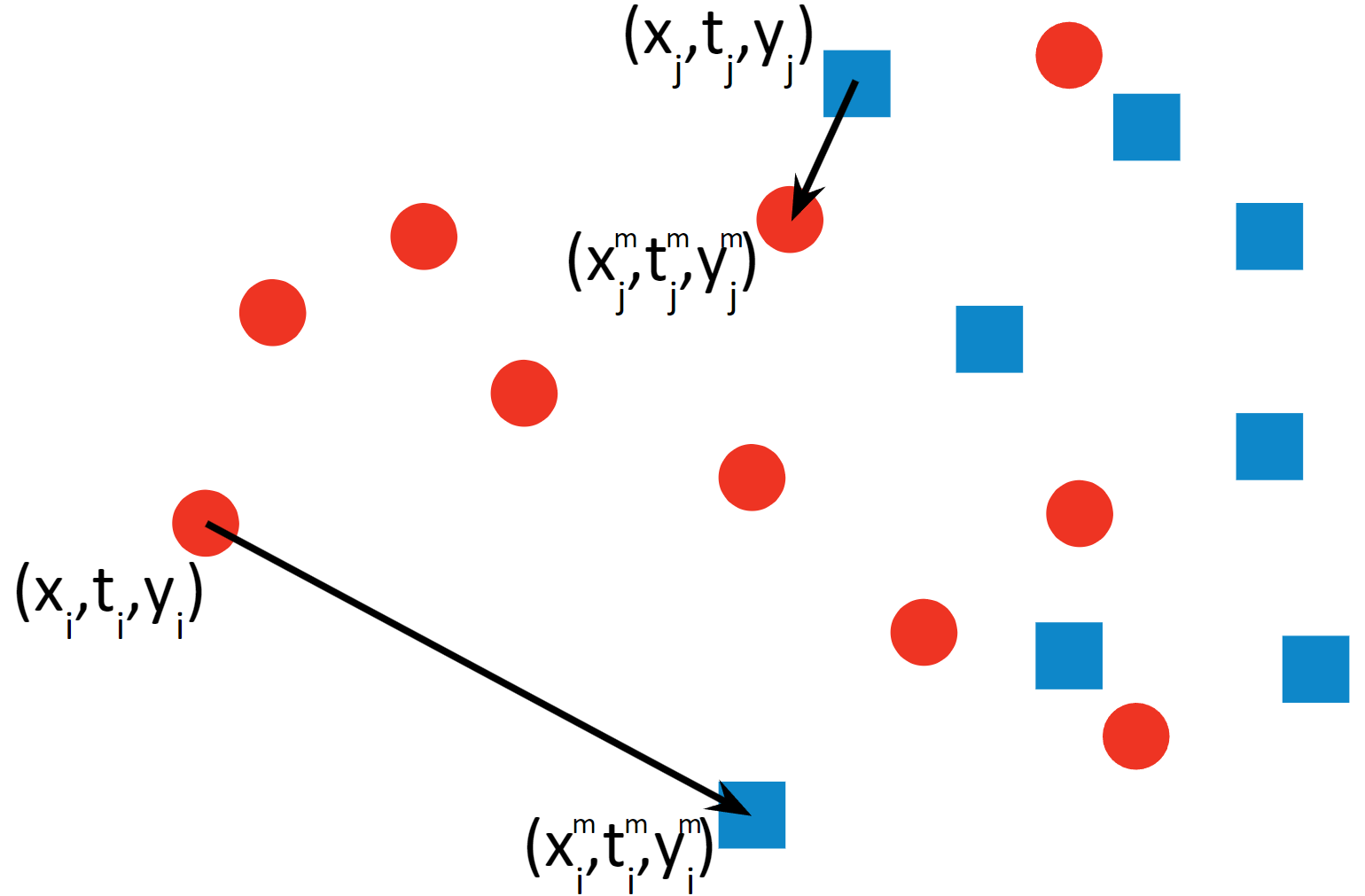
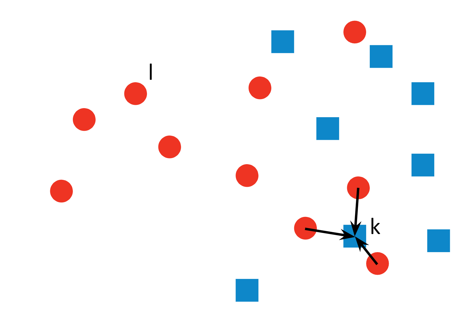
Figure 3: Treated and control samples in latent space. Left: the treated $x_{i}$ has a far mirror twin; the control $x_{j}$ has a close mirror twin. Right: the treated $x_{\ell}$ has counter-factual importance weight 0; the control sample $x_{k}$ has $w_{k}$=3.

The notions of latent mirror twin, and counterfactual importance weight are used to estimate the quality of the latent space. Informally speaking, a latent space allowing good counterfactual estimation of the treated samples is such that: i) the treated examples are close to their mirror twin; ii) the $\mu^{0}(x)\approx\mathbb{E}[Y|T=0,X=x]$ model learned on this latent space is of good quality, especially for control $x_{j}$ with a high $w_{j}$ (since the quality of $\mu_{0}(x_{j})$ has an impact on the counterfactual estimation of many treated $x_{i}$).

Formally, a pipeline $\mathcal{P}=(\phi,h^{0},h^{1})$ is defined as the triplet formed by an embedding $\phi$ mapping the instance space on some latent space ($\phi:\mathcal{X}\rightarrow\mathcal{Z}\subset\mathbb{R}^{d}$) and models $h^{0}$ and $h^{1}$ of the treated and control outcome ($h^{t}:\mathcal{Z}\rightarrow\mathbb{R}$). Note that pipeline $\mathcal{P}$ constitutes a $T$-learner and yields a CATE estimate defined as:

$$\tau(x)=h^{1}\circ\phi(x)-h^{0}\circ\phi(x)$$

3.2.2 Model architecture

As said (Section 3.1), the accurate counter-factual estimate of samples requires these samples to be counter-factualizable, i.e. close to their mirror twins. As depicted on Fig. 1 however, the requirements of control and treated samples being counter-factualizable are not necessarily satisfied by the same change of representation.

Consequently, we consider two latent spaces, aimed at ensuring counterfactualization of treated and control samples. More formally, the treatment-driven pipeline $\mathcal{P}_{1}$ focuses on CATE for treated samples, while the control-driven pipeline $\mathcal{P}_{0}$ focuses on CATE for control samples.

The combination of the CATE estimates built from $\mathcal{P}_{0}$ and $\mathcal{P}_{1}$ is classically defined as:

$$\hat{\tau}:x\in\mathcal{X}\mapsto(1-\mbox{$\hat{\eta}$}(x))\hat{\tau}_{0}(x)+\mbox{$\hat{\eta}$}(x)\hat{\tau}_{1}(x)$$ (4)

with $\mbox{$\hat{\eta}$}(x)$ estimating the propensity score $P(T=1|X=x)$ and $\hat{\tau}_{0}$ and $\hat{\tau}_{1}$ denoting the CATE estimates derived from pipelines $\mathcal{P}_{1}$ and $\mathcal{P}_{0}$.

Note that Alrite bridges the gap between $T$-learners and $X$-learners: each pipeline ($\mathcal{P}_{0}$ and $\mathcal{P}_{1}$) defines a $T$-learner and a causal estimate; these causal estimates are combined as in X-learners (Eq. 4).

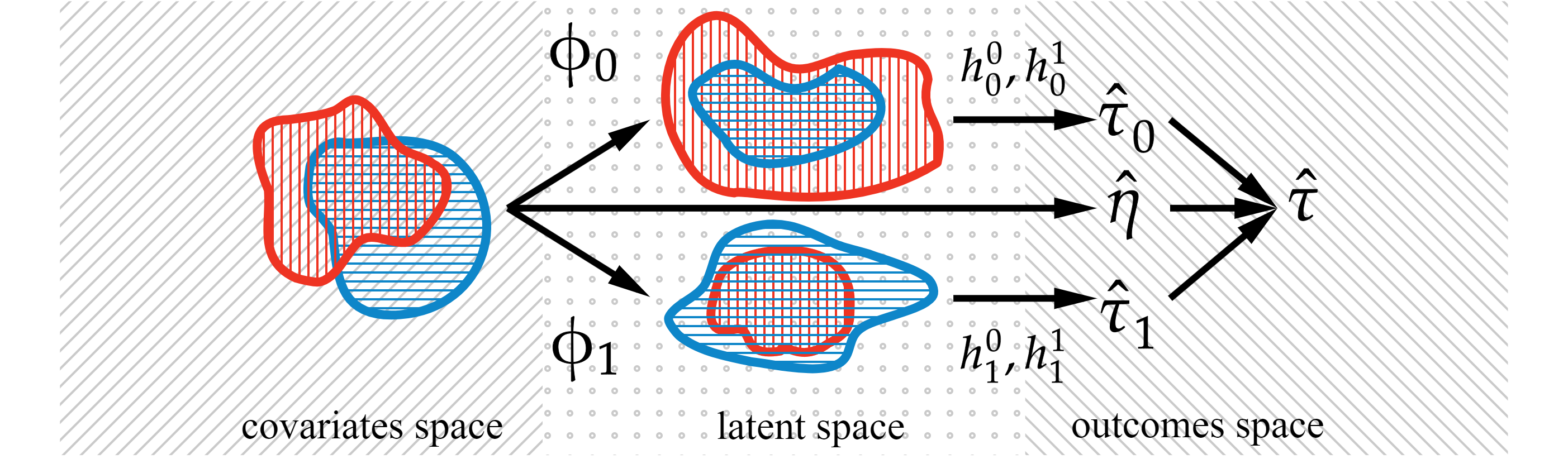
Figure 4: Alrite architecture: Top: control-driven pipeline $\mathcal{P}_{0}$. Middle: propensity estimate $\hat{\eta}$. Bottom: treatment-driven pipeline $\mathcal{P}_{1}$. Right: overall CATE estimate.

3.2.3 Training loss

Let us present the loss used to train control pipeline $\mathcal{P}_{0}$= $(\phi,h^{0},h^{1})$ (the $\mathcal{P}_{1}$ loss follows by symmetry). $\mathcal{P}_{0}$ is trained end-to-end by minimizing a compound loss enforcing: i) the accuracy of model $h^{0}$ on the control samples; ii) the accuracy of model $h^{1}$ on the treated samples (accounting for the fact that control samples with high counterfactual importance weight matter more); iii) the good counter-factualizability of control samples (a small distance to their mirror twin); iv) the regularization of the whole pipeline vector weight noted $\|\mbox{$\mathcal{P}_{0}$}\|$:

$$\begin{split}{\cal L}(\mbox{$\mathcal{P}_{0}$})=&\frac{1}{n_{0}}\sum_{t_{i}=0}(y_{i}-h^{0}(\phi(x_{i})))^{2}+\frac{1}{n_{1}+\beta n_{0}}\sum_{t_{i}=1}(1+\beta\mbox{$w_{i}$})(y_{i}-h^{1}(\phi(x_{i})))^{2}\\ &+\alpha\frac{1}{n_{0}}\sum_{t_{i}=0}\|\phi(x_{i})-\phi({x_{i}^{m}})\|^{2}+\gamma\|\mbox{$\mathcal{P}_{0}$}\|^{2}\end{split}$$ (5)

with $n_{0}$ and $n_{1}$ the number of control and treated samples in $\cal D$, $w_{i}$ the counterfactual importance weight of $x_{i}$, and $\alpha,\beta,\gamma$ hyper-parameters of the approach.

3.3 Algorithm

The Alrite algorithm finally involves three modules: learning $\mathcal{P}_{0}$ (Eq. 5); learning $\mathcal{P}_{1}$; learning the propensity estimate $\hat{\eta}$. Finally, the CATE estimates derived from $\mathcal{P}_{0}$ and $\mathcal{P}_{1}$ are aggregated using $\hat{\eta}$ (Eq. 4).

Algorithm 1 Alrite

Dataset $\mathcal{D}$; hyper-parameters $\alpha,\beta,\gamma$.

Learn $\mathcal{P}_{0}$= $(\phi_{0},h_{0}^{0},h_{0}^{1})$ (Eq. 5)

Compute $\hat{\tau}_{0}$

Learn $\mathcal{P}_{1}$= $(\phi_{1},h_{1}^{0},h_{1}^{1})$

Compute $\hat{\tau}_{1}$

Learn $\hat{\eta}$ // Propensity score

Compute $\hat{\tau}$ (Eq. 4)

As said, the propensity score $\hat{\eta}$ can be learned using classical supervised learning. Formally, a cross-entropy loss is used:

$$\mathcal{L}(\mbox{$\hat{\eta}$})=-\frac{1}{n_{1}}\sum_{t_{i}=1}\textit{log}\big{(}\mbox{$\hat{\eta}$}(x_{i})\big{)}-\frac{1}{n_{0}}\sum_{t_{i}=0}\textit{log}\big{(}1-\mbox{$\hat{\eta}$}(x_{i})\big{)}+\|\mbox{$\hat{\eta}$}\|^{2}$$ (6)

with $\|\mbox{$\hat{\eta}$}\|^{2}$ a regularization term. It is desirable that $\hat{\eta}$ be calibrated (Zadrozny and Elkan,, 2002), i.e. such that

$$\forall s\in[0,1],\ \mathbb{E}[T=1|\mbox{$\hat{\eta}$}(X)=s]=s$$

However the sensitivity of the overall $\hat{\tau}$ (defined by aggregating the CATE estimates $\hat{\tau}_{0}$ and $\hat{\tau}_{1}$ respectively derived from $\mathcal{P}_{0}$ and $\mathcal{P}_{1}$, Eq. 4) w.r.t. the propensity score is limited. Let $\tau_{\eta}$ denote the aggregation of $\hat{\tau}_{0}$ and $\hat{\tau}_{1}$ using the ground truth $\eta$. It reads:

$$||\hat{\tau}-\hat{\tau}_{\eta}|| =||(\mbox{$\hat{\eta}$}-\eta)(\hat{\tau}_{0}-\hat{\tau}_{1})||$$ (7)

$$\leq||\mbox{$\hat{\eta}$}-\eta||\times\big{(}\|\hat{\tau}_{0}-\tau\|+\|\hat{\tau}_{1}-\tau\|\big{)}$$

In other words, the CATE error due to the error on $\eta$ is of order 2, as the product of i) the error on the propensity; ii) the error on $\hat{\tau}_{0}$ and on $\hat{\tau}_{1}$.

Remark: It is straightforward to define an ensemble variant of Alrite, by splitting the dataset into a training, a validation, and a test dataset. On the training subset, several pipelines $\mathcal{P}_{0}$ and $\mathcal{P}_{1}$ are learned using different hyper-parameter settings. The best pipelines (determined from their factual accuracy on the validation set) are selected and they are aggregated to form the ensemble CATE model. The aggregation is the average of the top-K out of all pipelines, with $K$ a hyper-parameter of the ensemble approach, or a weighted sum, where the weight of each model corresponds to a softmax of hyper-parameter $\lambda$ (Appendix C).

3.4 Formal guarantees

As said, a main contribution of the approach is to provide formal guarantees on the PEHE error of Alrite, considering the within-sample setting, i.e. when the treatment variable $T$ is known. Remind that the within-sample error is not trivial $-$ contrarily to the training error in supervised learning $-$ as counter-factual $Y^{1-T}$ is not observed. All proofs are given in Appendix A.1. Our first result states that the PEHE loss associated with a T-learner is upper bounded depending on the counter-factualizability of the samples.

Theorem 1.

Let $\phi:\mathcal{X}\rightarrow\mathcal{Z}$ be an embedding from $\mathcal{X}$ to a latent space $\mathcal{Z}$. Let us assume that the sought outcome models $\mu^{0}$ and $\mu^{1}$ can be expressed as $\mu^{0}=\nu^{0}\circ\phi$ and $\mu^{1}=\nu^{1}\circ\phi$, with $\nu^{0}$ and $\nu^{1}$ two functions defined on $\mathcal{Z}$ with Lipschitz constant $L$.
Let $\mbox{$\hat{\nu}$}^{0},\mbox{$\hat{\nu}$}^{1}:\mathcal{Z}\rightarrow\mathbb{R}$ be two models trained to approximate $\nu^{0}$ and $\nu^{1}$ with Lipschitz constant $\hat{L}$. Then the empirical PEHE associated with $(\mbox{$\hat{\nu}$}^{1}\ -\mbox{$\hat{\nu}$}^{0})\circ\phi$ is upper bounded by $M_{1}$ with:

$$M_{1}=\frac{4}{n}\Big{[}\sum_{i=1}^{n}\Big{(}1+\mbox{$w_{i}$}\Big{)}\Big{(}(\mbox{$\hat{\nu}$}^{t_{i}}\circ\phi)(x_{i})-y_{i}\Big{)}^{2}+(L^{2}+\hat{L}^{2})\sum_{i=1}^{n}\|x_{i}-{x_{i}^{m}}\|^{2}\Big{]}$$

Bound $M_{1}$ depends on two terms: i) the factual accuracy on every sample $x_{i}$, all the more important the higher its counter-factual importance weight $w_{i}$, and ii) the counter-factualizability of the samples. This bound establishes the soundness of the training loss (Eq. 5), built on both terms.

Building on this result, our second result concerns the hybrid X-learnerT-learner scheme of Alrite.

Theorem 2.

Let $\mathcal{P}_{0}$ and $\mathcal{P}_{1}$ be a control and a treatment pipeline, respectively involving embeddings $\phi_{0}$ and $\phi_{1}$. Let us further assume that the sought outcome models $\mu^{0}$ and $\mu^{1}$ can be expressed on the top of each embedding ($\mu^{0}=\nu_{0}^{0}\circ\phi_{0}=\nu_{1}^{0}\circ\phi_{1}$ and $\mu^{1}=\nu_{1}^{0}\circ\phi_{0}=\nu_{1}^{1}\circ\phi_{1}$), with all $\nu_{i}^{j}$ of Lipschitz constant $L$ for $i,j\in\{0,1\}$.
Let $h_{0}^{0}$ and $h_{0}^{1}$ (respectively $h_{1}^{0}$ and $h_{1}^{1}$) denote the learned models of $\nu_{0}^{0}$ and $\nu_{0}^{1}$ in $\mathcal{P}_{0}$ (resp. $\nu_{1}^{0}$ and $\nu_{1}^{1}$ in $\mathcal{P}_{1}$), with Lipschitz constant $\hat{L}$.

For any $i$-th sample in the observation dataset $\cal D$, define

$$\bar{\tau}_{i}=(1-t_{i})\big{(}(h_{0}^{1}\circ\phi_{0})(x_{i})-y_{i}\big{)}+t_{i}\big{(}y_{i}-(h_{1}^{0}\circ\phi_{1})(x_{i})\big{)}$$

Let us further define the counter-factual importance weight of sample $(x_{j},t_{j},y_{j})$ as the number of samples $(x_{i},t_{i},y_{i})$ such that $t_{i}=1-t_{j}$ and $x_{i}$ is the nearest neighbor of $x_{j}$ according to $\phi_{t_{i}}$:

$$\mbox{$w_{j}$}=\#\{(x_{i},t_{i},y_{j})\in\mathcal{D}\ s.t.\ (x_{j},t_{j},y_{j})=(x_{i}^{m,\phi_{t_{i}}},1-t_{i},y_{i}^{m,\phi_{t_{i}}})\}$$

Then, the within-sample PEHE defined by $\frac{1}{n}\sum_{i=1}^{n}\big{(}\bar{\tau}_{i}-\tau(x_{i})\big{)}^{2}$ is upper bounded by $M_{2}$, with

$$M_{2}=\frac{5}{n}\Big{[}\sum_{t_{i}=1,i=1}^{n}\mbox{$w_{i}$}\bigl{(}(h_{0}^{1}\circ\phi_{0})(x_{i})-y_{i}\bigr{)}^{2}+\sum_{t_{i}=0,i=1}^{n}\mbox{$w_{i}$}((h_{1}^{0}\circ\phi_{1})(x_{i})-y_{i})^{2}+(L^{2}+\hat{L}^{2})\sum_{i=1}^{n}\|\phi_{t_{i}}(x_{i})-\phi_{t_{i}}(x_{i}^{m,\phi_{t_{i}}})\|^{2}+\kappa_{Y}\Big{]}$$

where $\kappa_{Y}=\sum_{i=1}^{n}\big{(}1+\mbox{$w_{i}$}\big{)}\big{(}y_{i}-\mu^{t_{i}}(x_{i})\big{)}^{2}$.

As said, Thm. 2 holds in the within-sample setting, as it requires knowledge of the treatment assignment $T$. It does not generalize directly to the out-of-sample setting, where the (unknown) $t_{i}$ and $y_{i}$ are respectively estimated using the propensity and the outcome models.

Finally, the upper-bound established in Thm. 2 is directly related with the loss used to train the pipelines (Eq. 5), establishing the well-foundedness of the approach, as follows:

Theorem 3.

There exists a hyper-parameter setting $(\mbox{$\alpha_{\scriptsize{0}}$},\mbox{$\alpha_{\scriptsize{1}}$},\mbox{$\beta_{\scriptsize{0}}$},\mbox{$\beta_{\scriptsize{1}}$})$ such that the within-sample empirical PEHE is upper bounded by $M_{3}$, with:

$$M_{3}= 5\Big{[}{\cal L}(\mbox{$\mathcal{P}_{1}$})+{\cal L}(\mbox{$\mathcal{P}_{0}$})-\gamma_{0}\|\mbox{$\mathcal{P}_{0}$}\|-\gamma\|\mbox{$\mathcal{P}_{1}$}\|+\kappa_{Y}$$

$$-\frac{1}{n_{0}}\sum_{t_{i}=0,i=1}^{n}(h_{0}^{0}\circ\phi_{0}(x_{i})-y_{i})^{2}-\frac{1}{n_{1}}\sum_{t_{i}=1,i=1}^{n}(h_{1}^{1}\circ\phi_{1}(x_{i})-y_{i})^{2}$$

$$-\frac{1}{n}\big{(}\sum_{t_{i}=0,i=1}^{n}(h_{1}^{0}\circ\phi_{1}(x_{i})-y_{i})^{2}+\sum_{t_{i}=1,i=1}^{n}(h_{0}^{1}\circ\phi_{0}(x_{i})-y_{i})^{2}\big{)}\Big{]}$$

Note that this result is not constructive in the sense that it does not give the hyper-parameter setting. Nevertheless, the relation between this bound on the PEHE and the terms in the pipeline loss confirms the soundness of the approach. This bound also depends on the Lipschitz constants of the learned models and of the target models (which only depend on the problem).

3.5 Discussion

The formal guarantees established by Thm 1-3 contrast with the main result of Shalit et al. Shalit et al., (2017) in two ways.

Theorem (from Shalit et al., (2017)).

Let $(\phi,h^{0},h^{1})$ be a pipeline such that $\phi:\mathcal{X}\rightarrow\mathcal{Z}$ is invertible. Define the point-wise loss function $\ell_{h,\phi}$ and expected factual loss $\epsilon_{t}$ conditionally to treatment assignment $T=t,\ t\in\{0,1\}$ by $$\begin{cases}\ell_{h,\phi}:(x,t)\in\mathcal{X}\times\{0,1\}&\mapsto\mathbb{E}[\big{(}Y^{t}-h\circ\phi(x)\big{)}^{2}|X=x]\\ \epsilon^{t}:h\in(\mathcal{Z}\rightarrow\mathcal{Y})&\mapsto\mathbb{E}[\ell_{h,\phi}(X,T)|T=t]\end{cases}$$ (8) Denote by $\sigma_{Y^{t}}^{2}=\mathbb{E}\big{[}(Y^{t}-\mathbb{E}[Y^{t}|X])^{2}|T=t\big{]}\mathbb{P}(T=t)$ the expected variance of $Y^{t}$, $t\in\{0,1\}$. Let G be a family of functions $\mathcal{Z}\rightarrow\mathcal{Y}$. Assume that there exists a constant $B_{\phi}>0$ such that $z\in\mathcal{Z}\mapsto\frac{1}{B_{\phi}}\ell_{h^{t},\phi}(\phi^{-1}(z),t)\in G$, $t\in\{0,1\}$. Denote the integral probability metric between the control and treated latent distributions induced by $\phi$ as $$\textit{IPM}=\sup_{g\in G}\big{|}\mathbb{E}\big{[}\big{(}\mathbb{P}\big{(}\phi(X)|T\text{=}1\big{)}-\mathbb{P}\big{(}\phi(X)|T\text{=}0\big{)}\big{)}g\big{(}\phi(X)\big{)}\big{]}\big{|}$$ Then, the PEHE is upper bounded: $$\textit{PEHE}(\phi,h^{0},h^{1})\leq 2\big{(}\epsilon^{0}(h^{0})+\epsilon^{1}(h^{1})+B_{\phi}\times\textit{IPM}-2\min(\sigma_{Y^{0}}^{2},\sigma_{Y^{1}}^{2})\big{)}$$ A first difference is that Shalit et al., (2017) relies on the invertibility of embedding $\phi$. In contrast, Alrite only assumes that the considered embeddings $\phi$ are such that the sought models can be expressed with no loss of information (there exists $\nu^{0}$ and $\nu^{1}$ s.t. $\mu^{\ell}=\nu^{\ell}\circ\phi$). As a result, Alrite can fully benefit of the celebrated opportunities offered by a change of representation (Cayton,, 2008; Bengio et al.,, 2013), e.g. to achieve feature selection or dimensionality reduction.

A second difference is that the bound in Shalit et al., (2017) involves integral probability metrics, thus defined in the large sample limit case. In contrast, our results build upon the counter-factual importance weights and the counter-factualizability of the samples, that is, empirical quantities that are in principle more readily understood by a practitioner.

Another key issue concerns the efficiency of the loss, and whether the considered optimization problem admits the sought solution as optimum. Let us focus on the control model; the treatment model case follows by symmetry. Under the assumption that embedding $\phi$ is such that it entails no loss of information w.r.t. the sought models, i.e. there exists $\nu^{t}$ such that $\mu^{t}=\nu^{t}\circ\phi$, then the ground truth $\nu^{t}$ minimizes the factual error loss.

Lemma 4.

Under the assumption of conditional exchangeability, let embedding $\phi$ be such that there exists $\nu^{0}$ with $\mu^{0}=\nu^{0}\circ\phi$. For any candidate model $\mbox{$\hat{\nu}$}^{0}$, let ${\cal L}(\mbox{$\hat{\nu}$}^{0})$ denote the expected mean squared prediction error of $\mbox{$\hat{\nu}$}^{0}$ conditionally to $T=0$ :

$${\cal L}(\mbox{$\hat{\nu}$}^{0}) =\mathbb{E}_{X,Y|T=0}\big{[}\big{(}\mbox{$\hat{\nu}$}^{0}\circ\phi(X)-Y^{0}\big{)}^{2}|T=0\big{]}$$

$$=\mathbb{E}_{Z=\phi(X),Y|T=0}\big{[}\big{(}\mbox{$\hat{\nu}$}^{0}(Z)-Y\big{)}^{2}|T=0\big{]}$$

Then, $\nu^{0}$ reaches the minimum of $\cal L$.

Proof: in Appendix A.1. Note that from the practitioner’s viewpoint, it is impossible to prove that a given statistic is sufficient based only on observational data. Indeed if $\phi$ is injective then $Y^{0}\perp\!\!\!\perp X|\phi(X)$, but this result relies on mapping $\phi$, and not on the observational data itself. Even in the large sample limit and using adequate conditional independence statistical tests, one may prove at most independence of $Y^{0}$ and $X$ conditionally to $(\phi(X)=z,T=0)$, but not conditionally to $(\phi(X)=z)$ alone. This concern echoes the ones raised by the assumption of conditional exchangeability: assuming sufficiency based on observational data is a similar leap of faith.

Let us last discuss the limitations of the approach and its robustness. The synthetic data depicted on Fig. 5 illustrates the sensitivity of Alrite w.r.t. the violation of the positivity assumption: the rightmost samples of the bottom cluster are overwhelmingly treated, and the leftmost samples of the top one are mainly control. The average distance to the mirror twin is much better for $\phi$ set to the projection on the $x$-axis (Fig. 5, bottom right) than for $\phi=$Id (Fig. 5, bottom left). The former $\phi$ might thus correspond to a local minimum of the training loss due to the low counter-factualizability, at the expense of the factual accuracy of the learned models.

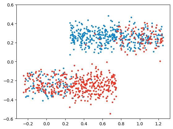
Figure 5: Distribution of the control and treated samples. Top: covariate space $\mathbb{R}^{2}$. Bottom left: distribution of distances to mirror twins for $\phi=$Id. Bottom right: distribution of distances to mirror twins for $\phi=$projection on the $x$-axis.

Another potential weakness of the approach is due to the impact of samples with high counter-factual importance weight. The compound loss (Eq. 5) focuses on optimizing the factual accuracy for samples with a high weight. A risk is to distort the optimization of $\phi$, in such a way that samples that are hard to model have a low counter-factual importance weight. This risk is mitigated as the gradient does not flow back through the mirror twin operator during the back-propagation phase; there should be no incentive for the optimization process to distort $\phi$ in such a pathological way. Further research is concerned with defining a smoother counter-factual importance weight.

4 Experimental validation

After describing the two benchmarks we considered, IHDP  and ACIC2016, and the experimental setting, this section reports on the empirical validation of Alrite. The Alrite code is publicly available.

4.1 Benchmarks

The IHDP dataset is the baseline dataset commonly used for benchmarking causal inference models (Shalit et al.,, 2017; Du et al.,, 2021; Zhou et al.,, 2021). The ACIC2016 benchmark originates from the 2016 Atlantic Causal Inference Challenge (Dorie et al.,, 2017).

4.1.1 IHDP

The IHDP dataset, introduced by Hill, (2011), is based on a real-life randomized experiment dataset, the Infant Health and Development Program (Brooks-Gunn et al.,, 1992). The treatment consists of quality child care and home visits on the health and development of preterm children. While the treatment assignment is randomized in the collected data, treatment imbalance is enforced by Hill, (2011), by removing a subpopulation (treated group children with non-white mothers) from the dataset.

The dataset contains $747$ individuals, $139$ of whom are treated; these are described by 25 covariate features, among which 6 are continuous and 19 binary.

The major difference between the original survey results and Hill, (2011)’s IHDP dataset lies in the replacement of the initial outcome with simulated outcomes, making it possible to access counter-factual quantities and ensuring that conditional exchangeability holds. The selected simulation method consists in defining two response surfaces $\mu^{t}:x\in\mathcal{X}\mapsto\mathbb{E}[Y^{t}|X=x],t\in\{0,1\}$, to which Gaussian noise is added.

We consider the IHDP-100 benchmark, involving 100 datasets (referred to as problem instance or instance when no confusion is to fear), where each dataset is generated by: i) drawing $\beta$ in $[0,1]^{25}$; ii) setting the surface responses as:

$$Y^{0} \sim\exp\{\langle X+0.5,\beta\rangle\}+\mathcal{N}(0,1)$$

$$Y^{1} \sim\langle X+0.5,\beta\rangle+\omega+\mathcal{N}(0,1),\mbox{ with $\omega$ s.t. average treatment effect }\textit{ATT}=4$$

Each dataset is split into a training (90% of samples) and a testing (10%) subset, the split being fixed to enable a fair comparison among the algorithms. Following the state of the art, 30% of the training set is held out to form a validation set.

The main performance indicators are the within-sample and out-of-sample PEHE, respectively computed on the training samples (where the treatment assignment and factual outcome are known, and the counter-factual outcome is unknown) and on the test set (where the treatment assignment and both outcomes are unknown). Following the state-of-the-art (Shalit et al.,, 2017; Du et al.,, 2021; Zhou et al.,, 2021), the results are averaged over the 100 datasets.

A secondary performance indicator on the IHDP benchmark is the mean absolute error on the ATE estimation $\epsilon_{\textit{ATE}}$ (Eq. 1). Note that ATE is notorious for being subject to systemic estimation bias: $\epsilon_{\textit{ATE}}$ favors low-bias models (as opposed to PEHE, that favors low-variance models).

Some criticisms have been presented in the literature concerning IHDP (Curth et al., 2021b, ):

Firstly, the ranges of outcomes and the causal effects are not commensurate among the different problem instances, as shown in Fig. 6(a). Likewise, the standard deviation of $\mu^{0}$ takes high values in some instances while it is generally low for $\mu^{1}$. As a result, $\tau$ widely varies depending on the problem instance, both in terms of average and variance.

A high standard deviation $\sigma_{\tau}$ of the causal effects makes CATE estimation more difficult: when $\sigma_{\tau}$ goes to $0$, the causal effect is uniform and the CATE estimation problem boils down to the (much simpler) ATE estimation problem. Quite the contrary, a large $\sigma_{\tau}$ makes large errors more likely. This claim is visually confirmed in Fig. 6-(f), plotting the standard deviations of $\tau$ vs the PEHE of the Alrite estimate $\hat{\tau}$ for all instances in IHDP-100. Interestingly, instances with large $\sigma_{\tau}$ account for a large fraction of the overall PEHE error. Accordingly, IHDP performance indicators strongly depend on how the algorithm behave on the few toughest instances; they do not reflect the average behavior of the algorithm.

(a) Average $\mu^{0}$ and $\mu^{1}$

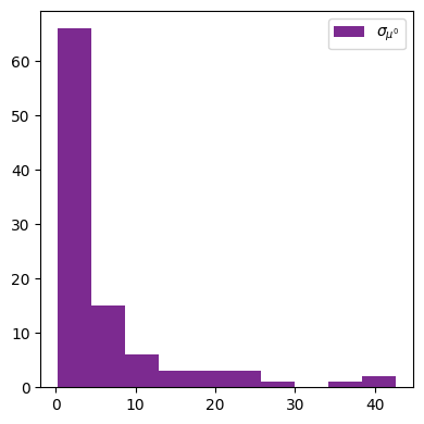
(b) Standard deviation of $\mu^{0}$

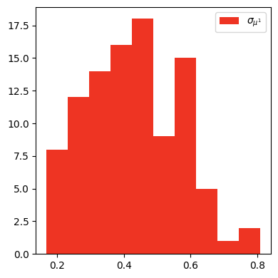
(c) Standard deviation of $\mu^{1}$

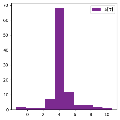
(d) Average treatment effect (ATT).

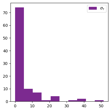
(e) Standard deviation $\sigma_{\tau}$ of ATT.

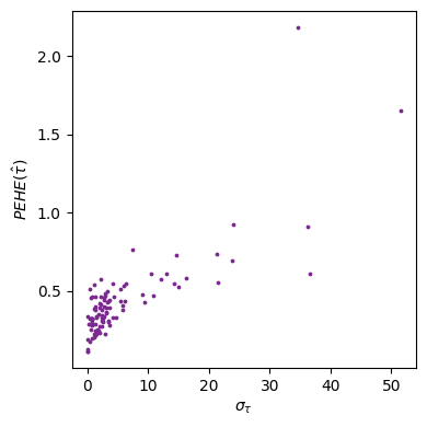
(f) $\textit{PEHE}(\hat{\tau})$ vs $\sigma_{\tau}$

Figure 6: Diversity of the 100 problem instances in IHDP-100: Histograms of effects and standard deviations, and relation between error PEHE and standard deviation $\sigma_{\tau}$.

4.1.2 ACIC2016

ACIC2016, designed for the 2016 Atlantic Causal Inference Challenge (Dorie et al.,, 2017), aims to compare different causal inference protocols. Like IHDP, ACIC2016 is a set of problem instances, generated as follows: $77$ data generation protocols are first defined. For each protocol, in order to limit the computational burden and in accordance with Zhang et al., (2021), we took into account the first $10$ generated datasets, i.e. a total of $770$ datasets.

Each dataset contains $4802$ samples, described by $58$ features derived from real-world data. Light, (1973) presents a longitudinal study carried out between years $1959$ and $1965$, with a view to identifying factors that affect the probability of children’s organic neurological defects. $23$ of the $58$ features are continuous, $27$ are counts, $5$ are binary and $3$ are categorical.

Like for IHDP, the treatment assignment and potential outcomes are simulated, ensuring that the conditional exchangeability, positivity, and SUTVA assumptions hold true. Data generation protocols Dorie et al., (2017) differ in their degree of nonlinearity, percentage of treatment assignment, overlap, alignment, treatment effect magnitude and heterogeneity, allowing a wide variety of situations to be described.

Formally the data generation process is of the form:

$$f:x\in\mathcal{X}\mapsto g\big{(}f_{1}(x_{1})+f_{2}(x_{2})+f_{3}(x_{1})f_{4}(x_{2})\big{)}$$

where the $f_{i}$ functions are either polynomial terms, step functions or indicator functions; the different features may be combined in various ways. The link function $g$ introduces a nonlinearity or bound the output. The outcome functions are defined as $Y^{t}\sim g_{t}(X)+\mathcal{N}$ with $\mathcal{N}$ a centered noise term; the propensity is defined as: $T\sim\textit{Ber}(f(X))$.

The performance indicator is PEHE, averaged over all $770$ instances of the ACIC2016 dataset.

As said, the ACIC2016 benchmark aims to overcome the limitations of common benchmark datasets (Dorie et al.,, 2017), while enabling to compute the PEHE. In particular, the choice to extract the covariates from real-life data avoids the potential data homogeneity of synthetic datasets. Despite the variety of the potential outcome models, the CATE is the difference between the two surface responses ($\tau=\mu^{1}-\mu^{0}$), thus favoring T-learners and S-learners.

4.2 Baselines

The baseline models considered to comparatively assess the performance of Alrite are listed in Table 1. It is emphasized that their results are those reported in the cited papers: In some cases, the code is not made public and there is a lack of details regarding the implementation; in other cases, there is a lack of details regarding the hyper-parameter setting; both prevent us from reproducing the results.

4.3 Alrite: Hyper-parameter setting

The detail of the hyper-parameters and computational framework is given in Appendix B. Pipelines $\mathcal{P}_{0}$ and $\mathcal{P}_{1}$ are trained independently, and implemented as neural networks with Exponential Linear Units (ELU) activation functions (Clevert et al.,, 2015).

The architecture hyper-parameters include the number $L$ of layers and the layer width $W$ (same for all layers), with normalization of the last layer of the embeddings and of the outcome models.

The training hyper-parameters include the initial learning rate, the batch size and the number of epochs. Training is conducted using Adam (Kingma and Ba,, 2014), with exponential weight decay. Overfitting is prevented using a validation set $\mathcal{D}_{\mathcal{V}}$ including $30\%$ of the training set, and using the factual error to select the model after a fixed number of epochs.

The propensity estimate is trained using mainstream supervised learning; logistic regression, k-nearest neighbors, and decision trees are considered. The model retained is determined by grid-search using a cross-validation scheme for each considered dataset.

4.4 Experimental results

The average performance of Alrite on all IHDP instances is reported on Table 1, compared with all other baselines. On this dataset, Alrite ranks first on within-sample PEHE and second on out-of-sample PEHE. Indeed, Alrite is designed to optimize the PEHE performance indicator, as motivated by Thm. 1. The comparatively lesser performance regarding within-sample and out-of-sample $\epsilon_{\textit{ATE}}$ is blamed on the $L_{2}$ regularization (more in Section 4.5), tending to bias the estimates toward 0, as noted by Laan and Rose, (2011).

As could be expected Breiman, (2001), ensemble variants of Alrite introduced in Section 3.3 improve on Alrite. The PEHE and (factual) accuracy depending on their hyperparameters (number $K$ of models in the top-$K$ ensemble, temperature $\lambda$ for the softmax weighted combination) are reported on Fig. 7 (one point per value of the hyperparameter).

This figure suggests that the factual accuracy can reliably be used to select the hyperparameter ($K=4$ for the top-K ensemble and $\lambda=100$ for the softmax ensemble) yielding the best PEHE. For these selected hyperparameters, the PEHE is statistically significantly better than Alrite with p-value$=1.3e-3$ on a one-sided paired t-test.

	IHDP
	within-sample		out-of-sample
	$\sqrt{\textit{PEHE}}$	$\epsilon_{\textit{ATE}}$	$\sqrt{\textit{PEHE}}$	$\epsilon_{\textit{ATE}}$
$\textit{OLS}_{2}$ Shalit et al., (2017)	$2.4\pm.1$	$.14\pm.01$	$2.5\pm.1$	$.31\pm.02$
BART Hill, (2011)	$2.1\pm.1$	$.23\pm.01$	$2.1\pm.1$	$.34\pm.02$
BNN Johansson et al., (2016)	$2.2\pm.1$	$.37\pm.03$	$2.1\pm.1$	$.42\pm.03$
CF Wager and Athey, (2018)	$3.8\pm.2$	$.18\pm.01$	$3.8\pm.2$	$.40\pm.03$
CFR-Wass Shalit et al., (2017)	$.71\pm.0$	$.25\pm.01$	$.76\pm.0$	$.27\pm.01$
CEVAE Louizos et al., (2017)	$2.7\pm.1$	$.34\pm.01$	$2.6\pm.1$	$.46\pm.02$
SITE Yao et al., (2018)	$.60\pm.09$	/	$.66\pm.11$	/
GANITE Yoon et al., (2018)	$1.9\pm.4$	$.43\pm.05$	$2.4\pm.4$	$.49\pm.05$
NSGP Alaa and Schaar, (2018)	$.51\pm.01$	/	$.64\pm.03$	/
ACE Yao et al., (2019)	$.49\pm.005$	/	$.54\pm.06$	/
DKLITE Zhang et al., (2020)	$.52\pm.02$	/	$.65\pm.03$	/
DR-CFR Hassanpour and Greiner, 2019b	/	/	$.65\pm.03$	$\textbf{.03}\pm.04$
BWCFR Assaad et al., (2021)	/	/	$.63\pm.01$	$.19\pm.01$
ABCEI Du et al., (2021)	$.71\pm.0$	$\textbf{.09}\pm.01$	$.73\pm.0$	$.09\pm.01$
CBRE Zhou et al., (2021)	$.52\pm.0$	$.10\pm.01$	$.60\pm.1$	$.13\pm.02$
MIM-DRCFR Cheng et al., (2022)	/	/	$\textbf{.38}\pm.009$	$.09\pm.001$
DeR-CFR Wu et al., 2023b	$.44\pm.02$	$.13\pm.02$	$.53\pm.07$	$.15\pm.02$
DRCFR+ Chauhan et al., (2023)	$.86\pm.01$	/	$1.19\pm.01$	/
Alrite	$.42\pm.03$	$.12\pm.009$	$.43\pm.02$	$.13\pm.01$
K-top Alrite	$\textbf{.40}\pm.02$	$.10\pm.008$	$.41\pm.02$	$.11\pm.009$
$\textit{softmax}_{\lambda}$ Alrite	$\textbf{.40}\pm.023$	$.095\pm.008$	$.42\pm.02$	$.11\pm.008$

Table 1: IHDP: Comparative performances of all baselines and Alrite (lower is better). Statistically significantly better results are indicated in bold.

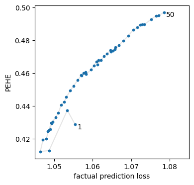
(a) $\hat{\tau}^{\textit{top-K}}$, $K\in\llbracket 1,50\rrbracket$, IHDP

(b) $\textit{softmax}_{\lambda}$, $\lambda\in\{10^{\nicefrac{{k}}{{2}}}\}_{k=2}^{16}$, IHDP

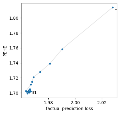
(c) $\hat{\tau}^{\textit{top-K}}$, $K\in\llbracket 1,31\rrbracket$, ACIC2016

(d) $\textit{softmax}_{\lambda}$, $\lambda\in\{10^{\nicefrac{{k}}{{2}}}\}_{k=\text{-}2}^{12}$, ACIC2016

Figure 7: Ensemble models in the out-of-sample setting: PEHE vs factual error on the validation set sensitivity, depending on the hyper-parameter.

Likewise, the average performance of Alrite on all ACIC2016 instances is reported on Table 2, compared with all other baselines. On this dataset, Alrite ranks second for PEHE both within-sample and out-of-sample, behind TEDVAE Zhang et al., (2021). A tentative interpretation for this fact is that some problem instances use a uniform treatment assignment, while other problem instances are truly unbalanced. However, by design Alrite is not suited to uniform treatment assignment: in such cases, it is not necessary to consider the counter-factualization of control and treatment samples independently. On the contrary, learning two separate pipelines, $\mathcal{P}_{1}$ and $\mathcal{P}_{0}$  is likely to lead to over-fitting. The issue is all the more severe as the selected hyper-parameter setting is the same for all ACIC2016 instances.

Most interestingly however, both ensemble variants of Alrite significantly improve on Alrite and on TEDVAE. It is reminded that the hyperparameters of the ensemble are selected (one value for all problem instances) as detailed in Appendix B.

	ACIC2016
	within-sample	out-of-sample
CF Athey and Imbens, (2016)	2.16 $\pm.17$	2.18 $\pm.18$
BART Hill, (2011)	2.13 $\pm.18$	2.17 $\pm.15$
X-learner(RF) Künzel et al., (2019)	1.86 $\pm.15$	1.89 $\pm.16$
CFR Shalit et al., (2017)	2.05 $\pm.18$	2.18 $\pm.20$
SITE Yao et al., (2018)	2.32 $\pm.19$	2.41 $\pm.23$
DR-CFR Hassanpour and Greiner, 2019b	2.44 $\pm.20$	2.56 $\pm.21$
GANITE Yoon et al., (2018)	3.12 $\pm.28$	3.28 $\pm.35$
CEVAE Louizos et al., (2017)	2.78 $\pm.56$	2.84 $\pm.61$
TEDVAE Zhang et al., (2021)	1.75 $\pm.14$	1.77 $\pm.17$
Alrite (ours)	1.79 $\pm.11$	1.81 $\pm.13$
K-top Alrite	1.69 $\pm.11$	1.70 $\pm.13$
$\textit{softmax}_{\lambda}$ Alrite	1.69 $\pm.11$	1.70 $\pm.13$

Table 2: Comparative performances of Alrite and baselines on ACIC2016. All baseline performances are reported from Zhang et al., (2021).

4.5 Discussion

As we said, the comparatively poorer performance of Alrite over ATE, compared to PEHE, is blamed on the regularization term (term $\gamma\|\mbox{$\mathcal{P}_{1}$}\|$ of the training loss, Eq. 5), which aims to avoid overfitting. This interpretation is confirmed by complementary experiments Lacombe, (2024).

5 Conclusion

The main contribution of the proposed approach lies in the observation that, when treatment assignment is not uniform, counterfactual estimation for control and treated samples induces two distinct problems. Alrite takes this observation into account through an original neural architecture, hybridizing X-learners and T-learners.

Two quantities are thus defined to characterize the quality of a change of representation: the counter-factualizability of a sample, i.e. its distance from its twin in latent space; and the weight of the counterfactual importance of a sample $x$, counting how many samples admit $x$ as a twin. Finally, the models are learned by optimizing a learning loss that imposes a good change of representation: the aim is to ensure good counter-factualizability of all samples, and to ensure that the factual model is all the more accurate on examples with higher counterfactual importance weights.

Learned models benefit from theoretical guarantees, noting that the upper bound ofPEHE involves the same terms as those involved in the learning loss. Last, the merits of the approach are experimentally demonstrated on the main two benchmarks of the domain, compared with the prominent approaches of the state of the art. A word of caution: the approach is not suited to uniform treatment assignment: in this case, the two counterfactual estimation problems are in fact the same, and the two-pipeline Alrite runs the risk of overfitting.

Several research perspectives are opened up by Alrite. One short-term perspective is to jointly learn both pipelines, thus promoting their complementarity.

Another perspective is to revise the notion of latent twin, which currently involves only the nearest neighbor of the sample under consideration. A more robust approach would be to consider several nearest neighbors of a sample in the latent space (e.g. using a Gaussian kernel) and revise the counterfactual importance weight of neighboring samples accordingly.

A third perspective concerns the notion of uncertainty. The minimization of CATE uncertainty is at the heart of the proposed change of representation, which aims to strengthen the counter-factualizability of samples. An alternative could be based on the different models involved in the Alrite ensemble, using them to assess uncertainty on factual and counterfactual estimates for any particular sample.

Lastly, the extension of the approach to the multi-level treatment setting can be tackled, considering one pipeline per treatment level, plus one for the control setting.

Appendix A Appendix

A.1 Proofs

A.1.1 Proof of Thm. 1

Proof.

Let $(x,t,y)$ be a sample in $\cal D$ with $z=\phi(x)$, and let $(x^{\prime},t^{\prime}=1-t,y^{\prime})$ be its mirror twin w.r.t $\phi$ ($\phi(x^{\prime})=z^{\prime}$). Assuming with no loss of generality that $t=1$, it comes:

$$|(\mbox{$\hat{\nu}$}^{1}\text{-}\mbox{$\hat{\nu}$}^{0})(z)-(\nu^{1}\text{-}\nu^{0})(z)|^{2}$$

$$=|[\mbox{$\hat{\nu}$}^{1}(z)\text{-}\nu^{1}(z)]-[\mbox{$\hat{\nu}$}^{0}(z)\text{-}\mbox{$\hat{\nu}$}^{0}(z^{\prime})]-[\mbox{$\hat{\nu}$}^{0}(z^{\prime})\text{-}\nu^{0}(z^{\prime})]-[\nu^{0}(z^{\prime})\text{-}\nu^{0}(z)]|^{2}$$

$$\leq 4|\mbox{$\hat{\nu}$}^{1}(z)\text{-}\nu^{1}(z)|^{2}+4|\mbox{$\hat{\nu}$}^{0}(z)\text{-}\mbox{$\hat{\nu}$}^{0}(z^{\prime})|^{2}+4|\mbox{$\hat{\nu}$}^{0}(z^{\prime})\text{-}\nu^{0}(z^{\prime})|^{2}+4|\nu^{0}(z^{\prime})\text{-}\nu^{0}(z)|^{2}$$

$$\leq 4|\mbox{$\hat{\nu}$}^{1}(z)\text{-}\nu^{1}(z)|^{2}+4|\mbox{$\hat{\nu}$}^{0}(z^{\prime})\text{-}\nu^{0}(z^{\prime})|^{2}+4(\widehat{L}^{2}+L^{2})||z^{\prime}\text{-}z||^{2}$$

Averaging over $(x,t,y)$ in $\cal D$ yields the result. ∎

A.1.2 Proof of Thm. 2

Proof.

Let $(x_{i},t_{i},y_{i})$ be a sample in $\cal D$. Without loss of generality, assume $t_{i}=1$. Let $(x_{j},t_{j}=0,y_{j})$ be its mirror twin. Denote by $z_{i}$ and $z_{j}$ their respective representations: $\phi_{1}(x_{i})=z_{i},\phi_{1}(x_{j})=z_{j}$. Using Cauchy-Schwarz applied on $\mathbb{R}^{5}$, for any vector $u\in\mathbb{R}^{5}$,

$$(\sum u_{i})^{2}\ =\langle\mathds{1},u\rangle^{2}\leq||\mathds{1}||^{2}\times||u||^{2}=5\sum u_{i}^{2}$$

with $\mathds{1}$ the vector with all coordinates set to 1. It then comes:

$$\big{(}\bar{\tau}_{i}-\tau(x_{i})\big{)}^{2}= \big{(}(y_{i}-\mbox{$h_{\scriptsize{1}}^{0}$}(z_{i}))-(\nu_{\scriptsize{1}}^{1}-\nu_{\scriptsize{1}}^{0})(z_{i})\big{)}^{2}$$

$$= \big{(}[y_{i}-\nu_{\scriptsize{1}}^{1}(z_{i})]+[\nu_{\scriptsize{1}}^{0}(z_{i})-\nu_{\scriptsize{1}}^{0}(z_{j})]+[\nu_{\scriptsize{1}}^{0}(z_{j})-y_{j}]$$

$$+[y_{j}-\mbox{$h_{\scriptsize{1}}^{0}$}(z_{j})]+[\mbox{$h_{\scriptsize{1}}^{0}$}(z_{j})-\mbox{$h_{\scriptsize{1}}^{0}$}(z_{i})]\big{)}^{2}$$

$$\leq 5(y_{i}-\nu_{\scriptsize{1}}^{1}(z_{i}))^{2}+5(\nu_{\scriptsize{1}}^{0}(z_{i})-\nu_{\scriptsize{1}}^{0}(z_{j}))^{2}+5(\nu_{\scriptsize{1}}^{0}(z_{j})-y_{j})^{2}$$

$$+5(y_{j}-\mbox{$h_{\scriptsize{1}}^{0}$}(z_{j}))^{2}+5(\mbox{$h_{\scriptsize{1}}^{0}$}(z_{j})-\mbox{$h_{\scriptsize{1}}^{0}$}(z_{i}))^{2}$$

$$\leq 5(y_{i}-\mu^{1}(x_{i}))^{2}+5(y_{j}-\mu^{0}(y_{j}))^{2}+5(y_{j}-\mbox{$h_{\scriptsize{1}}^{0}$}(z_{j}))^{2}+5(\widehat{L}^{2}+L^{2})||z_{j}-z_{i}||^{2}$$

Averaging over $(x_{i},t_{i}=1)$ in $\cal D$, it comes:

$$\frac{1}{n}\sum_{t_{i}=1}\big{(}\bar{\tau}_{i}-\tau(x_{i})\big{)}^{2}\leq\frac{5}{n} \sum_{t_{i}=1}\biggl{(}(L^{2}+\hat{L}^{2})\|\phi(x_{i})-\phi(x_{j})\|^{2}+\big{(}\mu^{1}(x_{i})-y_{i}\big{)}^{2}\biggl{)}$$

$$+\frac{5}{n} \sum_{t_{j}=0}\bigg{(}w_{j}\big{[}\big{(}h_{1}^{0}\circ\phi_{1}(x_{j})-y_{j}\big{)}^{2}+\big{(}\mu^{0}(x_{j})-y_{j}\big{)}^{2}\big{]}\bigg{)}$$

Adding the control samples sum yields $M_{2}$. ∎

A.1.3 Proof of Thm. 3

Proof.

Set the loss hyper-parameters values $\mbox{$\alpha_{\scriptsize{0}}$},\mbox{$\alpha_{\scriptsize{1}}$},\mbox{$\beta_{\scriptsize{0}}$},\mbox{$\beta_{\scriptsize{1}}$}$ to

$$\big{(}\mbox{$\alpha_{\scriptsize{0}}$},\mbox{$\alpha_{\scriptsize{1}}$},\mbox{$\beta_{\scriptsize{0}}$},\mbox{$\beta_{\scriptsize{1}}$}\big{)} =\big{(}(1-p)(L^{2}+\hat{L}^{2}),p(L^{2}+\hat{L}^{2}),1,1\big{)}$$

entailing

$$\big{(}\frac{\mbox{$\alpha_{\scriptsize{0}}$}}{n_{0}},\frac{\mbox{$\alpha_{\scriptsize{1}}$}}{n_{1}},\frac{\mbox{$\beta_{\scriptsize{0}}$}}{n_{1}+\mbox{$\beta_{\scriptsize{0}}$}n_{0}},\frac{\mbox{$\beta_{\scriptsize{1}}$}}{n_{0}+\mbox{$\beta_{\scriptsize{1}}$}n_{1}}\big{)} =\big{(}\frac{L^{2}+\hat{L}^{2}}{n},\frac{L^{2}+\hat{L}^{2}}{n},\frac{1}{n},\frac{1}{n}\big{)}$$

Then, the total loss over both pipelines total loss writes

$$\mbox{$\mathcal{L}(\mbox{$\mathcal{P}_{0}$})$}\text{+}\mbox{$\mathcal{L}(\mbox{$\mathcal{P}_{1}$})$}= \Bigg{(}\frac{L^{2}+\hat{L}^{2}}{n}\sum_{t_{i}=0}\|\phi_{0}(x_{i})-\phi_{0}(x_{i}^{m,\phi_{0}})\|^{2}+\frac{1}{n}\sum_{t_{i}=1}w_{i}(\mbox{$h_{\scriptsize{0}}^{1}$}\circ\phi_{0}(x_{i})\text{-}y_{i})^{2}\Bigg{)}$$

$$+\Bigg{(}\frac{1}{n(1\text{-}p)}\sum_{t_{i}=0}(\mbox{$h_{\scriptsize{0}}^{0}$}\circ\phi_{0}(x_{i})\text{-}y_{i})^{2}+\frac{1}{n}\sum_{t_{i}=1}(\mbox{$h_{\scriptsize{0}}^{1}$}\circ\phi_{0}(x_{i})\text{-}y_{i})^{2}+\mbox{$\gamma_{\scriptsize{0}}$}\Omega(\mbox{$\mathcal{P}_{0}$})\Bigg{)}$$

$$+\Bigg{(}\frac{L^{2}+\hat{L}^{2}}{n}\sum_{t_{i}=1}\|\phi_{1}(x_{i})-\phi_{1}(x_{i}^{m,\phi_{1}})\|^{2}+\frac{1}{n}\sum_{t_{i}=0}w_{i}(\mbox{$h_{\scriptsize{1}}^{0}$}\circ\phi_{1}(x_{i})\text{-}y_{i})^{2}\Bigg{)}$$

$$+\Bigg{(}\frac{1}{np}\sum_{t_{i}=1}(\mbox{$h_{\scriptsize{1}}^{1}$}\circ\phi_{1}(x_{i})\text{-}y_{i})^{2}+\frac{1}{n}\sum_{t_{i}=0}(\mbox{$h_{\scriptsize{1}}^{0}$}\circ\phi_{1}(x_{i})\text{-}y_{i})^{2}+\mbox{$\gamma_{\scriptsize{1}}$}\Omega(\mbox{$\mathcal{P}_{1}$})\Bigg{)}$$

$$= \frac{1}{n}\sum_{t_{i}=0}\biggl{(}w_{i}\big{(}h_{1}^{0}\circ\phi_{1}(x_{i})\text{-}y_{i}\big{)}^{2}+(L^{2}+\hat{L}^{2})\|\phi_{0}(x_{i})-\phi_{0}(x_{i}^{m,\phi_{0}})\|^{2}\biggl{)}$$

$$+ \frac{1}{n}\sum_{t_{i}=1}\biggl{(}w_{i}\big{(}h_{0}^{1}\circ\phi_{0}(x_{i})\text{-}y_{i}\big{)}^{2}+(L^{2}+\hat{L}^{2})\|\phi_{1}(x_{i})-\phi_{1}(x_{i}^{m,\phi_{1}})\|^{2}\biggl{)}$$

$$+\frac{1}{n}\sum_{i=1}^{n}(h_{1-t_{i}}^{t_{i}}\circ\phi_{1-t_{i}}(x_{i})\text{-}y_{i})^{2}+\frac{1}{n}\sum_{i=1}^{n}\frac{(h_{t_{i}}^{t_{i}}\circ\phi_{t_{i}}(x_{i})\text{-}y_{i})^{2}}{t_{i}p+(1\text{-}t_{i})(1\text{-}p)}+\mbox{$\gamma_{\scriptsize{0}}$}\Omega(\mbox{$\mathcal{P}_{0}$})+\mbox{$\gamma_{\scriptsize{1}}$}\Omega(\mbox{$\mathcal{P}_{1}$})$$

$$= \frac{1}{5}M_{2}-\kappa_{Y}+\mbox{$\gamma_{\scriptsize{0}}$}\Omega(\mbox{$\mathcal{P}_{0}$})+\mbox{$\gamma_{\scriptsize{1}}$}\Omega(\mbox{$\mathcal{P}_{1}$})$$

$$+\frac{1}{n}\sum_{i=1}^{n}(h_{1-t_{i}}^{t_{i}}\circ\phi_{1-t_{i}}(x_{i})\text{-}y_{i})^{2}+\frac{1}{n}\sum_{i=1}^{n}\frac{(h_{t_{i}}^{t_{i}}\circ\phi_{t_{i}}(x_{i})\text{-}y_{i})^{2}}{t_{i}p+(1\text{-}t_{i})(1\text{-}p)}$$

implying an upper bound on the within-sample empirical PEHE:

$$\frac{1}{n}\sum_{i=1}^{n}\big{(}\bar{\tau}_{i}-\tau(x_{i})\big{)}^{2} \leq 5\big{(}\mbox{$\mathcal{L}(\mbox{$\mathcal{P}_{0}$})$}+\mbox{$\mathcal{L}(\mbox{$\mathcal{P}_{1}$})$}\big{)}-5\big{(}\mbox{$\gamma_{\scriptsize{0}}$}\|\mbox{$\mathcal{P}_{0}$}\|^{2}+\mbox{$\gamma_{\scriptsize{1}}$}\|\mbox{$\mathcal{P}_{1}$}\|^{2}\big{)}+5\kappa_{Y}$$

$$-\frac{5}{n}\sum_{i=1}^{n}\frac{1}{p^{t_{i}}}(h_{t_{i}}^{t_{i}}\circ\phi_{t_{i}}(x_{i})-y_{i})^{2}-\frac{5}{n}\sum_{i=1}^{n}(h_{1-t_{i}}^{t_{i}}\circ\phi_{1-t_{i}}(x_{i})-y_{i})^{2}$$

∎

A.1.4 Proof of Lemma 4

Proof.

Let $\nu^{0*}$ be a minimizer of ${\cal L}(\cdot)=\mathbb{E}_{X,Y|T=0}\big{[}\big{(}\cdot\circ\phi(X)-Y^{0}\big{)}^{2}|T=0\big{]}$. Then, $\nu^{0*}:z\in\mathcal{Z}\mapsto\mathbb{E}[Y^{0}|T=0,\phi(X)=z]$ and therefore $\nu^{0*}\circ\phi:x\in\mathcal{X}\mapsto\mathbb{E}[Y^{0}|T=0,\phi(X)=\phi(x)]$. The problem rephrases in: does the equality of $\mathbb{E}[Y^{0}|T=0,\phi(X)=\phi(\cdot)]$ and $\mu^{0}(\cdot)$ hold?

Let us first show that the average value of the control outcome $Y^{0}$ conditionally on $X$ equals the average value conditionally on $\phi(X)$. Let then $x$ be an element of $\mathcal{X}$. Denote by $U$ the set of events $\phi^{-1}(\{\phi(x)\})$. The formula of total probability writes

$$\mathbb{E}[Y^{0}|\phi(X)=\phi(x)] =\int\nolimits_{U}\mathbb{E}[Y^{0}|\phi(X)=\phi(x),X=u]\mathbb{P}(X=u|\phi(X)=\phi(x))\textit{du}$$

$$=\int\nolimits_{U}\mathbb{E}[Y^{0}|X=u]\mathbb{P}(X=u|\phi(X)=\phi(x))\textit{du}$$

$$=\int\nolimits_{U}\mu^{0}(u)\mathbb{P}(X=u|\phi(X)=\phi(x))\textit{du}$$

$$=\int\nolimits_{U}\nu^{0}\circ\phi(u)\mathbb{P}(X=u|\phi(X)=\phi(x))\textit{du}$$

$$=\int\nolimits_{U}\nu^{0}\circ\phi(x)\mathbb{P}(X=u|\phi(X)=\phi(x))\textit{du}$$

$$=\nu^{0}\circ\phi(x)\int\nolimits_{U}\mathbb{P}(X=u|\phi(X)=\phi(x))\textit{du}$$

$$=\mu^{0}(x)$$

Now let us show that $\mathbb{E}[Y^{0}|\phi(X)=\phi(\cdot)]$ and $\mathbb{E}[Y^{0}|T=0,\phi(X)=\phi(\cdot)]$ are also equal. Denote by $V$ the set of events $(\phi(X),T)^{-1}(\{(\phi(x),0)\})$. Then,

$$\mathbb{E}[Y^{0}|\phi(X)=\phi(x),T=0] =\int\nolimits_{V}\mathbb{E}[Y^{0}|\phi(X)=\phi(x),T=0,X=v]\mathbb{P}(X=v|\phi(X)=\phi(x),T=0)\textit{dv}$$

$$=\int\nolimits_{V}\mathbb{E}[Y^{0}|T=0,X=v]\mathbb{P}(X=v|\phi(X)=\phi(x),T=0)\textit{dv}$$

$$=\int\nolimits_{V}\mathbb{E}[Y^{0}|X=v]\mathbb{P}(X=v|\phi(X)=\phi(x),T=0)\textit{dv}$$

$$=\int\nolimits_{V}\mathbb{E}[Y^{0}|\phi(X)=\phi(x)]\mathbb{P}(X=v|\phi(X)=\phi(x),T=0)\textit{dv}\ \hskip 20.0pt\textit{(cf. above)}$$

$$=\mathbb{E}[Y^{0}|\phi(X)=\phi(x)]\int_{V}\mathbb{P}(X=v|\phi(X)=\phi(x),T=0)\textit{dv}$$

$$=\mathbb{E}[Y^{0}|\phi(X)=\phi(x)]$$

Finally, $\mathbb{E}[Y^{0}|T=0,\phi(X)=\phi(\cdot)]=\mu^{0}(\cdot)$, and $\nu^{0}$ minimizes $\mathcal{L}$. ∎

A.2 Additional remarks regarding the discussion of the formal analysis (Section 3.5)

Although the main result of Shalit et al., (2017) resorts to the invertibility of the mapping $\phi$, strictly weaker assumptions allow for $\nu^{0}$ to reach the minimum of $\mathcal{L}$. In particular, if $\phi$ is injective, then conditioning on $X=x$ is equivalent to conditioning on $\phi(X)=\phi(x)$, and the equality $\mathbb{E}[Y^{0}|T=0,\phi(X)=\phi(\cdot)]=\mu^{0}(\cdot)$ directly follows.

The equality still holds in the strictly weaker setting where $\phi(X)$ is a sufficient statistic with respect to $Y^{0}$, in the sense that $Y^{0}\perp\!\!\!\perp X|\phi(X)$.

Finally, as shown by Lemma 4, the equality still holds under the strictly weaker hypothesis that there exists $\nu^{0}$ such that $\mu^{0}=\nu^{0}\circ\phi$.

Note that the hypothesis $Y^{0}\perp\!\!\!\perp T|\phi(X)$ isn’t sufficient nor necessary.

A.2.1 Asymptotical behavior of insulation

Given a mapping $\phi$ and in the large sample limit, the insulation of any sample goes to 0 in probability.

Proof.

Let us assume for simplicity that $\mathcal{X}\subset\mathbb{R}^{d}$. Let $(x_{i},t_{i}=0,y_{i})$ be a control sample from the training dataset $\mathcal{D}$, with $\epsilon>0$. Function $\phi_{0}$, being implemented with a finite-weights neural network, is continuous. As such, the inverse image of the latent space open ball $\textit{B}(\phi_{0}(x_{i}),\epsilon)$ centered on $\phi_{0}(x_{i})$ with radius $\epsilon$ is also an open. $(x_{i},t_{i}=0,y_{i})$ has been sampled from $\mathbb{P}_{X,T,Y}$ and belongs to $\phi_{0}^{-1}(\textit{B}(\phi_{0}(x_{i}),\epsilon))$ so there also exists an open $A\subset\phi_{0}^{-1}(\textit{B}(\phi_{0}(x_{i}),\epsilon))$ of $\mathbb{R}^{d}$ such that $\mathbb{P}(T=0,X\in B)>0$. Since positivity holds, $\mathbb{P}(T=1,X\in A)>0$. Finally,

$$\mathbb{P}\big{(}\|\phi_{0}(x_{i})-\phi_{0}({x_{i}^{m}})\|>\epsilon\big{)} =\mathbb{P}\big{(}\forall j\in\llbracket 1,n\rrbracket,\ t_{j}=1\ \implies\ \phi_{0}(x_{j})\not\in\ \textit{B}(\phi_{0}(x_{i}),\epsilon)\big{)}$$

$$\leq\mathbb{P}\big{(}\forall i\in\llbracket 1,n\rrbracket,\ t_{j}=1\ \implies\ x_{j}\not\in\ \phi_{0}^{-1}(\textit{B}(\phi_{0}(x_{i}),\epsilon))\big{)}$$

$$\leq\mathbb{P}\big{(}\forall j\in\llbracket 1,n\rrbracket,\ t_{j}=1\ \implies\ x_{j}\not\in\ A\big{)}$$

$$\leq\big{(}1-\mathbb{P}(T=1,X\in A)\big{)}^{n}$$

$$\xrightarrow{n\rightarrow+\infty}0$$

∎

Appendix B Hyper-parameter selection in causal inference

Alrite hyper-parameters are summarized in Table 3, together with their range of variation and the selected values for benchmarks IHDP and ACIC2016.

		IHDP		ACIC2016
	Range	$\mathcal{P}_{0}$	$\mathcal{P}_{1}$	$\mathcal{P}_{0}$	$\mathcal{P}_{1}$
regularization strength $\alpha$	$\{0\}\cup\ \{10^{k/2}\}_{k=-4}^{4}$	$10^{0}$	$10^{1.5}$	$10^{-2}$	$10^{-2}$
reweighting importance $\beta$	$\{0\}\cup\ \{10^{k/2}\}_{k=-4}^{2}$	$10^{-1.5}$	$0$	$10^{0}$	$0$
embedding model layers	$\llbracket 1,5\rrbracket$	$4$	$4$	$5$	$5$
outcome model layers	$\llbracket 1,5\rrbracket$	$3$	$4$	$5$	$5$
embedding model width	$\{20,50,100,200\}$	$20$	$20$	$100$	$100$
outcome model width	$\{20,50,100,200\}$	$50$	$100$	$100$	$100$
batch size	$\{50,100,200,500\}$	$200$	$200$	$250$	$250$

Table 3: Alrite: Range of variation for the hyper-parameters, and selected hyper-parameters values.

The selection of the hyper-parameter setting, referred to as the AutoML problem in the mainstream supervised learning framework (Hutter et al.,, 2019), is all the more severe in the CATE framework as the counterfactual information is de facto unknown; it thus prevents the usual performance indicators (PEHE) from being computed on any validation set $\mathcal{D}_{\mathcal{V}}$ sampled from the observational dataset $\cal D$.

The state of the art mostly relies on a model-dependent methodology, e.g., Athey and Imbens, (2016) for causal trees, Powers et al., (2018) for causal boosting and bagged causal multivariate adaptive regression splines, or Alaa and Van Der Schaar, (2018) for Gaussian processes.

The approach proposed in this paper aims to be model-agnostic. It builds upon: i) defining a proxy metric that can be computed on the validation set; ii) retaining the model optimizing the considered proxy metric. The proxy metric thus plays the same role as a surrogate PEHE. Following (Shalit et al.,, 2017), many authors rely on using $\mbox{$\tau${-risk}}_{\textit{1NNI}}$ as a proxy metric (detailed below). However, the 1-nearest neighbor estimator is known for its poor performance in middle to high-dimensional settings.

A set of proxy metrics has thus been considered (Table 4), and these metrics have been compared along several performance indicators to select the most robust one.

B.1 Proxy metrics

We distinguish:

• the $\mu$-risks, only measuring the (possibly reweighted) factual validation prediction error;

• the R-risk, based on the ‘Robinson’s transformation’ (Robinson,, 1988) (Eq. 2), that approximates $\mathbb{E}\big{[}\big{(}Y-m(X)-(T-\eta(X))\hat{\tau}(X)\big{)}^{2}\big{]}$ through approximating the mean conditional outcome $m(x)=\mathbb{E}[Y|X=x]$ and the propensity $\eta$;

• the $\tau$-risks, leveraging an independent approximation of the ground-truth CATE, that is most often based on a plug-in referred to as One Nearest-Neighbor Imputation (1NNI) (Shalit et al.,, 2017; Du et al.,, 2021; Zhou et al.,, 2021), where the counter-factual outcome of $x$ is approximated by the factual outcome of its closest neighbor with opposite treatment assignment in instance space, noted $\overline{(x,t,y)}$.

Estimator	Motivation	Expression: $\frac{1}{|\mathcal{D}_{\mathcal{V}}|}\sum_{(x,t,y)\in\mathcal{D}_{\mathcal{V}}}\bullet$
$\widehat{\mbox{$\mu${-risk}}}$	factual error	$\big{(}y-\mbox{$\hat{\mu}$}^{t}(x)\big{)}^{2}$
$\widehat{\mbox{$\mu${-risk}}}_{\textit{IPTW}}$	same + IPTW	$\mbox{$\hat{\varrho}$}^{t}(x)\big{(}y-\mbox{$\hat{\mu}$}^{t}(x)\big{)}^{2}$
$\widehat{\textit{R-risk}}$	R-learners	$\Big{(}\hat{\tau}(x)\big{(}t-\mbox{$\hat{\eta}$}(x)\big{)}-\big{(}y-\hat{m}(x)\big{)}\Big{)}^{2}$
$\widehat{\mbox{$\tau${-risk}}}_{\textit{naive}}$	simplicity	$\big{(}\hat{\tau}(x)-(\mbox{$\hat{\mu}$}^{1}(x)-\mbox{$\hat{\mu}$}^{0}(x))\big{)}^{2}$
$\widehat{\mbox{$\tau${-risk}}}_{\textit{1NNI}}$	1NNI	$\big{(}\hat{\tau}(x)-(2t-1)(y-\overline{(x,t,y)})\big{)}^{2},$
$\widehat{\mbox{$\tau${-risk}}}_{\textit{IPTW}}$	F-learners	$\big{(}\hat{\tau}(x)-(2t-1)\mbox{$\hat{\varrho}$}^{t}(x)y\big{)}^{2}$
$\widehat{\mbox{$\tau${-risk}}}_{\textit{U}}$	U-learners	$\big{(}\hat{\tau}(x)-(2t-1)\mbox{$\hat{\varrho}$}^{1-t}(x)\big{(}y-\hat{m}(x)\big{)}\big{)}^{2}$
$\widehat{\mbox{$\tau${-risk}}}_{\textit{DR}}$	double robustness	$\Big{(}\hat{\tau}(x)-\big{(}(\mbox{$\hat{\mu}$}^{1}\text{-}\mbox{$\hat{\mu}$}^{0})(x)+(2t-1)\mbox{$\hat{\varrho}$}^{t}(x)\big{(}y-\mbox{$\hat{\mu}$}^{t}(x)\big{)}\big{)}\Big{)}^{2}$

Table 4: Proxy metrics; $\hat{\varrho}$ denotes the inverse of the approximate propensity $\hat{\eta}$.

Some of the above-mentioned proxy metrics may rely on auxiliary models that provide independent estimates of the outcome functions $\mu^{0}$, $\mu^{1}$, mean outcome $m$ and the propensity $\eta$.
Models $\mbox{$\hat{\mu}$}^{0},\mbox{$\hat{\mu}$}^{1},\hat{m}$ are enforced by Nu-Support Vector Regressors (NuSVR) models (Platt,, 2000), since they achieve low high cross-validation factual prediction loss.
Propensity estimators are logistic regressions, k-nearest neighbors, or decision tree regressors. These estimators and their hyper-parameters are chosen through a classical cross-validation procedure.

B.2 Selecting a proxy metrics

On each benchmark, two sets of respectively $\ell_{\scriptsize{0}}$ and $\ell_{\scriptsize{1}}$ hyper-parameter settings are randomly sampled, defining a total of $C=\ell_{\scriptsize{0}}\times\ell_{\scriptsize{1}}$ candidate estimates

$$\hat{\tau}^{(\ell,\ell^{\prime})}=(1-\mbox{$\hat{\eta}$})\hat{\tau}_{\scriptsize{0}}^{(\ell)}+\mbox{$\hat{\eta}$}\ \hat{\tau}_{\scriptsize{1}}^{(\ell^{\prime})}$$

For each $j$-th candidate model ($j=1\ldots C$), its PEHE on the validation set noted $u_{j}$ is compared with the value of the proxy metrics, noted $v_{j}$. The reliability of the proxy metrics is assessed along three performance indicators: the Spearman correlation; the Kendall rank correlation (Kendall,, 1938); and the discounted cumulative gain (DCG) (Järvelin and Kekäläinen,, 2002).

The values taken by the PEHE and the proxy metrics on the validation set of IHDP are visually displayed in Fig. 8. Informally speaking, an ideal proxy metrics would show up as a diagonal line, displaying the identity of the true and the surrogate PEHE, i.e. the proxy metrics. Fig. 8 thus suggests that $\widehat{\mbox{$\mu${-risk}}}$ and $\widehat{\mbox{$\tau${-risk}}}_{\textit{DR}}$ constitute the best proxy metrics.

Quantitatively, the reliability of each proxy metrics is measured using Spearman correlation, Kendall rank correlation and DCG in Table 5.

We underline that this comparison can only be done in retrospect, for in real-life cases no evaluation of the PEHE is possible.

(a) $\mu$-risk

(b) $\mbox{$\mu${-risk}}_{\textit{IPTW}}$

(c) R-risk

(d) $\mbox{$\pi${-risk}}_{\textit{IPTW}}$

(e) $\mbox{$\pi${-risk}}_{\textit{DR}}$

(f) $\mbox{$\tau${-risk}}_{\textit{1NNI}}$

(g) $\mbox{$\tau${-risk}}_{\textit{naive}}$

(h) $\mbox{$\tau${-risk}}_{\textit{IPTW}}$

(i) $\mbox{$\tau${-risk}}_{\textit{U}}$

(j) $\mbox{$\tau${-risk}}_{\textit{DR}}$

Figure 8: PEHE value (test set) vs proxy metrics (validation set) for IHDP.

score	$\epsilon_{\textit{ATE}}$	$\sqrt{\textit{PEHE}}$	Spearman	-DCG	Kendall
$\mu$-risk	0.131	0.431	0.969	-2.016	0.846
$\mbox{$\mu${-risk}}_{\textit{IPTW}}$	0.131	0.431	0.942	-2.014	0.798
$\mbox{$\pi${-risk}}_{\textit{IPTW}}$	0.139	0.672	0.366	-2.751	0.253
$\mbox{$\pi${-risk}}_{\textit{DR}}$	0.136	0.490	0.796	-2.239	0.598
R-risk	0.146	0.723	-0.064	-3.304	-0.049
$\mbox{$\tau${-risk}}_{\textit{naive}}$	0.125	0.496	0.858	-2.196	0.668
$\mbox{$\tau${-risk}}_{\textit{1NNI}}$	0.125	0.462	0.903	-2.070	0.729
$\mbox{$\tau${-risk}}_{\textit{IPTW}}$	0.141	0.581	0.282	-3.281	0.199
$\mbox{$\tau${-risk}}_{\textit{U}}$	0.183	1.320	-0.357	-5.924	-0.252
$\mbox{$\tau${-risk}}_{\textit{DR}}$	0.131	0.431	0.960	-1.985	0.825

Table 5: Hyper-parameter selection on IHDP. Columns 2-3 display the performance of the model selected using the proxy metrics in column 1 (the lower the better). The associated scores correlation metrics are reported in columns 4-6 (the higher the better).

These experiments validate a posteriori the relevance of $\mu$-risk as best proxy metrics, as it achieves the lowest PEHE and lowest ATE. The quality of the proxy metrics is also confirmed by its high Spearman correlation coefficient, Kendall rank correlation coefficient, and discounted cumulative gain.

The proxy metrics empirically selected in Shalit et al., (2017), $\mbox{$\tau${-risk}}_{\textit{1NNI}}$, also appears to be a reliable proxy, supporting a good model selection.

While $\mbox{$\mu${-risk}}_{\textit{IPTW}}$, $\mbox{$\pi${-risk}}_{\textit{DR}}$, $\mbox{$\tau${-risk}}_{\textit{naive}}$ and $\mbox{$\tau${-risk}}_{\textit{DR}}$ seem worthy in retrospect, R-risk, $\mbox{$\pi${-risk}}_{\textit{IPTW}}$, $\mbox{$\tau${-risk}}_{\textit{IPTW}}$ and $\mbox{$\tau${-risk}}_{\textit{U}}$ achieve poor selection performance.

Appendix C Ensemble Alrite models

As mentioned (Appendix B), the hyper-parameter selection task relies on learning $\ell_{0}$ models $\hat{\tau}_{\scriptsize{0}}$ and $\ell_{1}$ models $\hat{\tau}_{\scriptsize{1}}$. Instead of selecting the best model according to the proxy metrics (Section B.2), we can return the best ensemble model combining the elementary models. Two types of combination have been considered in the experiments.

C.1 Top-K ensemble

With no loss of generality, let us assume that the $\hat{\tau}_{\scriptsize{0}}^{(i)}$ (resp. the $\hat{\tau}_{\scriptsize{1}}^{(j)}$) models are sorted by decreasing $\mu$-risk. For $1\leq k\leq\ell_{0}$, let $\overline{\hat{\tau}_{\scriptsize{0}}}^{k}$ be defined as the average of the first $k$ $\hat{\tau}_{\scriptsize{0}}$ models:

$$\overline{\hat{\tau}_{\scriptsize{0}}}^{k}(x)=\frac{1}{k}\sum_{i=1}^{k}\hat{\tau}_{\scriptsize{0}}^{(i)}(x)$$

and let $\overline{\hat{\tau}_{\scriptsize{1}}}^{k}$ be likewise defined as the average of the first $k$ $\hat{\tau}_{\scriptsize{1}}$ models. The overall ensemble $\overline{\hat{\tau}}^{k}$, called top-K ensemble, is defined as:

$$\overline{\hat{\tau}}^{K}(x)=(1-\mbox{$\hat{\eta}$}(x))\,\overline{\hat{\tau}_{\scriptsize{0}}}^{K}(x)\,+\,\mbox{$\hat{\eta}$}(x)\,\overline{\hat{\tau}_{\scriptsize{1}}}^{K}(x)$$ (11)

The hyper-parameter $K$, with $1\leq K\leq\textit{min}(\ell_{0},\ell_{1})$, is likewise selected by optimizing the $\mu$-risk of the ensemble.

C.2 $\lambda$ ensemble

The second Alrite ensemble, called $\lambda$ ensemble, is based on the weighted sum of the elementary models, where the weight of the $i$-th model is given as the softmax of the associated $\mu$-risk. Accordingly, the weighted sum of the $\hat{\tau}_{\scriptsize{0}}$ models, noted $\hat{\tau}_{\scriptsize{0}}^{\lambda}$, is defined as:

$$\hat{\tau}_{\scriptsize{0}}^{\lambda}(x)=\frac{1}{\sum_{j=1}^{\ell_{0}}\exp\{-\lambda\times\mbox{$\mu${-risk}}(\hat{\tau}_{\scriptsize{0}}^{j})\}}\hskip 7.22743pt\sum_{i=1}^{\ell_{0}}\exp\{-\lambda\times\mbox{$\mu${-risk}}(\hat{\tau}_{\scriptsize{0}}^{i})\}\,\hat{\tau}_{\scriptsize{0}}^{i}(x)$$

with $\lambda>0$. The weighted sum of the $\hat{\tau}_{\scriptsize{1}}$ models, denoted $\hat{\tau}_{\scriptsize{1}}^{\lambda}$, is likewise defined. Finally the overall ensemble $\hat{\tau}^{\lambda}$ is defined as:

$$\hat{\tau}^{\lambda}(x)=(1-\mbox{$\hat{\eta}$}(x))\,\hat{\tau}_{\scriptsize{0}}^{\lambda}(x)\,+\,\mbox{$\hat{\eta}$}(x)\,\hat{\tau}_{\scriptsize{1}}^{\lambda}(x)$$

Parameter $\lambda$ is selected by maximizing the $\mu$-risk of the $\lambda$ ensemble.

References

- Abadi et al., (2016) Abadi, M., Barham, P., Chen, J., Chen, Z., Davis, A., Dean, J., Devin, M., Ghemawat, S., Irving, G., Isard, M., Kudlur, M., Levenberg, J., Monga, R., Moore, S., Murray, D. G., Steiner, B., Tucker, P., Vasudevan, V., Warden, P., Wicke, M., Yu, Y., and Zheng, X. (2016). TensorFlow: a system for large-scale machine learning. In Proceedings of the 12th USENIX conference on Operating Systems Design and Implementation, OSDI’16, pages 265–283, USA. USENIX Association.
- Alaa and Schaar, (2018) Alaa, A. and Schaar, M. (2018). Limits of Estimating Heterogeneous Treatment Effects: Guidelines for Practical Algorithm Design. In Proceedings of the 35th International Conference on Machine Learning, pages 129–138. PMLR. ISSN: 2640-3498.
- Alaa and Van Der Schaar, (2018) Alaa, A. M. and Van Der Schaar, M. (2018). Bayesian Nonparametric Causal Inference: Information Rates and Learning Algorithms. IEEE Journal of Selected Topics in Signal Processing, 12(5):1031–1046.
- Angrist et al., (2009) Angrist, J. D., Pischke, J.-s., and Pischke, J.-s. (2009). Mostly Harmless Econometrics – An Empiricist‘s Companion. Princeton University Press, Princeton.
- Assaad et al., (2021) Assaad, S., Zeng, S., Tao, C., Datta, S., Mehta, N., Henao, R., Li, F., and Carin, L. (2021). Counterfactual Representation Learning with Balancing Weights. In Proceedings of The 24th International Conference on Artificial Intelligence and Statistics, pages 1972–1980. PMLR. ISSN: 2640-3498.
- Athey and Imbens, (2016) Athey, S. and Imbens, G. (2016). Recursive partitioning for heterogeneous causal effects. Proceedings of the National Academy of Sciences, 113(27):7353–7360. Publisher: Proceedings of the National Academy of Sciences.
- Ben-David et al., (2006) Ben-David, S., Blitzer, J., Crammer, K., and Pereira, F. (2006). Analysis of Representations for Domain Adaptation. In Advances in Neural Information Processing Systems, volume 19. MIT Press.
- Bengio et al., (2013) Bengio, Y., Courville, A., and Vincent, P. (2013). Representation Learning: A Review and New Perspectives. IEEE transactions on pattern analysis and machine intelligence, 35:1798–1828.
- Breiman, (2001) Breiman, L. (2001). Random Forests. Machine Learning, 45(1):5–32.
- Brooks-Gunn et al., (1992) Brooks-Gunn, J., Liaw, F. R., and Klebanov, P. K. (1992). Effects of early intervention on cognitive function of low birth weight preterm infants. The Journal of Pediatrics, 120(3):350–359.
- Caron et al., (2022) Caron, A., Baio, G., and Manolopoulou, I. (2022). Estimating individual treatment effects using non‐parametric regression models: A review. Journal of the Royal Statistical Society Series A, 185(3):1115–1149. Publisher: Royal Statistical Society.
- Cayton, (2008) Cayton, L. (2008). Algorithms for manifold learning. Technical Report CS2008-0923, Department of Computer Science & Engineering, UC San Diego.
- Chauhan et al., (2023) Chauhan, V. K., Molaei, S., Tania, M. H., Thakur, A., Zhu, T., and Clifton, D. A. (2023). Adversarial De-confounding in Individualised Treatment Effects Estimation. In Proceedings of The 26th International Conference on Artificial Intelligence and Statistics, pages 837–849. PMLR. ISSN: 2640-3498.
- Cheng et al., (2022) Cheng, M., Liao, X., Liu, Q., Ma, B., Xu, J., and Zheng, B. (2022). Learning Disentangled Representations for Counterfactual Regression via Mutual Information Minimization. In Proceedings of the 45th International ACM SIGIR Conference on Research and Development in Information Retrieval, SIGIR ’22, pages 1802–1806, New York, NY, USA. Association for Computing Machinery.
- Cheng et al., (2020) Cheng, P., Hao, W., Dai, S., Liu, J., Gan, Z., and Carin, L. (2020). CLUB: A Contrastive Log-ratio Upper Bound of Mutual Information. In Proceedings of the 37th International Conference on Machine Learning, pages 1779–1788. PMLR. ISSN: 2640-3498.
- Chernozhukov et al., (2017) Chernozhukov, V., Chetverikov, D., Demirer, M., Duflo, E., Hansen, C., and Newey, W. (2017). Double/Debiased/Neyman Machine Learning of Treatment Effects. American Economic Review, 107(5):261–265.
- Clevert et al., (2015) Clevert, D.-A., Unterthiner, T., and Hochreiter, S. (2015). Fast and Accurate Deep Network Learning by Exponential Linear Units (ELUs). Under Review of ICLR2016 (1997).
- (18) Curth, A., Alaa, A. M., and van der Schaar, M. (2021a). Estimating Structural Target Functions using Machine Learning and Influence Functions. arXiv:2008.06461 [stat].
- Curth and Schaar, (2021) Curth, A. and Schaar, M. v. d. (2021). Nonparametric Estimation of Heterogeneous Treatment Effects: From Theory to Learning Algorithms. In Proceedings of The 24th International Conference on Artificial Intelligence and Statistics, pages 1810–1818. PMLR. ISSN: 2640-3498.
- (20) Curth, A., Svensson, D., Weatherall, J., and van der Schaar, M. (2021b). Really Doing Great at Estimating CATE? A Critical Look at ML Benchmarking Practices in Treatment Effect Estimation. Proceedings of the Neural Information Processing Systems Track on Datasets and Benchmarks, 1.
- Cuturi, (2013) Cuturi, M. (2013). Sinkhorn Distances: Lightspeed Computation of Optimal Transport. In Advances in Neural Information Processing Systems, volume 26. Curran Associates, Inc.
- Dorie et al., (2017) Dorie, V., Hill, J., Shalit, U., Scott, M., and Cervone, D. (2017). Automated versus Do-It-Yourself Methods for Causal Inference: Lessons Learned from a Data Analysis Competition. Statistical Science, 34.
- Du et al., (2021) Du, X., Sun, L., Duivesteijn, W., Nikolaev, A., and Pechenizkiy, M. (2021). Adversarial balancing-based representation learning for causal effect inference with observational data. Data Mining and Knowledge Discovery, 35(4):1713–1738.
- Foster and Syrgkanis, (2023) Foster, D. J. and Syrgkanis, V. (2023). Orthogonal statistical learning. The Annals of Statistics, 51(3):879–908. Publisher: Institute of Mathematical Statistics.
- Ganin et al., (2016) Ganin, Y., Ustinova, E., Ajakan, H., Germain, P., Larochelle, H., Laviolette, F., March, M., and Lempitsky, V. (2016). Domain-Adversarial Training of Neural Networks. Journal of Machine Learning Research, 17(59):1–35.
- Goodfellow et al., (2014) Goodfellow, I., Pouget-Abadie, J., Mirza, M., Xu, B., Warde-Farley, D., Ozair, S., Courville, A., and Bengio, Y. (2014). Generative Adversarial Nets. In Advances in Neural Information Processing Systems, volume 27. Curran Associates, Inc.
- Gouk et al., (2021) Gouk, H., Frank, E., Pfahringer, B., and Cree, M. J. (2021). Regularisation of neural networks by enforcing Lipschitz continuity. Machine Learning, 110(2):393–416.
- Gretton et al., (2012) Gretton, A., Borgwardt, K. M., Rasch, M. J., Schölkopf, B., and Smola, A. (2012). A Kernel Two-Sample Test. Journal of Machine Learning Research, 13(25):723–773.
- Guo et al., (2023) Guo, X., Zhang, Y., Wang, J., and Long, M. (2023). Estimating heterogeneous treatment effects: mutual information bounds and learning algorithms. In Proceedings of the 40th International Conference on Machine Learning, volume 202 of ICML’23, pages 12108–12121, Honolulu, Hawaii, USA. JMLR.org.
- Hampel et al., (1986) Hampel, F. R., Ronchetti, E. M., Rousseeuw, P. J., and Stahel, W. A. (1986). Robust Statistics: The Approach Based on Influence Functions. Wiley–Blackwell, New York.
- (31) Hassanpour, N. and Greiner, R. (2019a). CounterFactual Regression with Importance Sampling Weights. In Proceedings of the Twenty-Eighth International Joint Conference on Artificial Intelligence, pages 5880–5887, Macao, China. International Joint Conferences on Artificial Intelligence Organization.
- (32) Hassanpour, N. and Greiner, R. (2019b). Learning Disentangled Representations for CounterFactual Regression. In Proceedings of The 8th International Conference on Learning Representations.
- Hill, (2011) Hill, J. L. (2011). Bayesian Nonparametric Modeling for Causal Inference. Journal of Computational and Graphical Statistics, 20(1):217–240.
- Hirano and Imbens, (2005) Hirano, K. and Imbens, G. W. (2005). The Propensity Score with Continuous Treatments. In Gelman, A. and Meng, X.-L., editors, Wiley Series in Probability and Statistics, pages 73–84. John Wiley & Sons, Ltd, Chichester, UK.
- Holland, (1986) Holland, P. W. (1986). Statistics and Causal Inference. Journal of the American Statistical Association, 81(396):945–960. Publisher: Taylor & Francis _eprint: https://www.tandfonline.com/doi/pdf/10.1080/01621459.1986.10478354.
- Hutter et al., (2019) Hutter, F., Kotthoff, L., and Vanschoren, J., editors (2019). Automated Machine Learning: Methods, Systems, Challenges. The Springer Series on Challenges in Machine Learning. Springer International Publishing, Cham.
- Johansson, (2023) Johansson, F. D. (2023). cfrnet. original-date: 2016-07-12T10:29:44Z.
- Johansson et al., (2022) Johansson, F. D., Shalit, U., Kallus, N., and Sontag, D. (2022). Generalization Bounds and Representation Learning for Estimation of Potential Outcomes and Causal Effects. arXiv:2001.07426 [cs, stat].
- Johansson et al., (2016) Johansson, F. D., Shalit, U., and Sontag, D. (2016). Learning representations for counterfactual inference. In Proceedings of the 33rd International Conference on International Conference on Machine Learning - Volume 48, ICML’16, pages 3020–3029, New York, NY, USA. JMLR.org.
- Järvelin and Kekäläinen, (2002) Järvelin, K. and Kekäläinen, J. (2002). Cumulated gain-based evaluation of IR techniques. ACM Transactions on Information Systems, 20(4):422–446.
- Kendall, (1938) Kendall, M. G. (1938). A New Measure of Rank Correlation. Biometrika, 30(1/2):81–93. Publisher: [Oxford University Press, Biometrika Trust].
- Kennedy, (2023) Kennedy, E. H. (2023). Towards optimal doubly robust estimation of heterogeneous causal effects. arXiv:2004.14497 [math, stat].
- Kingma and Ba, (2014) Kingma, D. and Ba, J. (2014). Adam: A Method for Stochastic Optimization. International Conference on Learning Representations.
- Kingma and Welling, (2014) Kingma, D. and Welling, M. (2014). Auto-Encoding Variational Bayes. In Proceedings of The 2nd International Conference on Learning Representations.
- Kuang et al., (2017) Kuang, K., Cui, P., Li, B., Jiang, M., Yang, S., and Wang, F. (2017). Treatment Effect Estimation with Data-Driven Variable Decomposition. Proceedings of the AAAI Conference on Artificial Intelligence, 31(1). Number: 1.
- Kuang et al., (2022) Kuang, K., Cui, P., Zou, H., Li, B., Tao, J., Wu, F., and Yang, S. (2022). Data-Driven Variable Decomposition for Treatment Effect Estimation. IEEE Transactions on Knowledge and Data Engineering, 34(5):2120–2134. Conference Name: IEEE Transactions on Knowledge and Data Engineering.
- Künzel et al., (2019) Künzel, S. R., Sekhon, J. S., Bickel, P. J., and Yu, B. (2019). Meta-learners for Estimating Heterogeneous Treatment Effects using Machine Learning. Proceedings of the National Academy of Sciences, 116(10):4156–4165. arXiv:1706.03461 [math, stat].
- Laan and Rose, (2011) Laan, M. J. v. d. and Rose, S. (2011). Targeted Learning: Causal Inference for Observational and Experimental Data. Springer Science & Business Media. Google-Books-ID: RGnSX5aCAgQC.
- Lacombe, (2024) Lacombe, A. (2024). Changes of representation for counter-factual inference. PhD thesis, Université Paris-Saclay. Thèse de doctorat dirigée par Sebag, Michèle et Caillou, Philippe Informatique université Paris-Saclay 2024.
- Lechner, (1999) Lechner, M. (1999). Earnings and Employment Effects of Continuous Gff-the-Job Training in East Germany After Unification. Journal of Business & Economic Statistics, 17(1):74–90. Publisher: Taylor & Francis _eprint: https://doi.org/10.1080/07350015.1999.10524798.
- Light, (1973) Light, I. J. (1973). The Collaborative Perinatal Study of the National Institute of Neurological Diseases and Stroke: The Women and Their Pregnancies. American Journal of Diseases of Children, 125(1):146.
- Louizos et al., (2017) Louizos, C., Shalit, U., Mooij, J. M., Sontag, D., Zemel, R., and Welling, M. (2017). Causal Effect Inference with Deep Latent-Variable Models. In Advances in Neural Information Processing Systems, volume 30. Curran Associates, Inc.
- Nie and Wager, (2021) Nie, X. and Wager, S. (2021). Quasi-oracle estimation of heterogeneous treatment effects. Biometrika, 108(2):299–319.
- Oprescu et al., (2023) Oprescu, M., Dorn, J., Ghoummaid, M., Jesson, A., Kallus, N., and Shalit, U. (2023). B-learner: quasi-oracle bounds on heterogeneous causal effects under hidden confounding. In Proceedings of the 40th International Conference on Machine Learning, volume 202 of ICML’23, pages 26599–26618, Honolulu, Hawaii, USA. JMLR.org.
- Pedregosa et al., (2011) Pedregosa, F., Varoquaux, G., Gramfort, A., Michel, V., Thirion, B., Grisel, O., Blondel, M., Prettenhofer, P., Weiss, R., Dubourg, V., Vanderplas, J., Passos, A., Cournapeau, D., Brucher, M., Perrot, M., and Duchesnay, E. (2011). Scikit-learn: Machine Learning in Python. Journal of Machine Learning Research, 12(85):2825–2830.
- Platt, (2000) Platt, J. (2000). Probabilistic Outputs for Support Vector Machines and Comparisons to Regularized Likelihood Methods. Adv. Large Margin Classif., 10.
- Powers et al., (2018) Powers, S., Qian, J., Jung, K., Schuler, A., Shah, N. H., Hastie, T., and Tibshirani, R. (2018). Some methods for heterogeneous treatment effect estimation in high dimensions. Statistics in Medicine, 37(11):1767–1787.
- Rezende et al., (2014) Rezende, D. J., Mohamed, S., and Wierstra, D. (2014). Stochastic Backpropagation and Approximate Inference in Deep Generative Models. In Proceedings of the 31st International Conference on Machine Learning, pages 1278–1286. PMLR. ISSN: 1938-7228.
- Robinson, (1988) Robinson, P. M. (1988). Root-N-Consistent Semiparametric Regression. Econometrica : journal of the Econometric Society, 56(4):931. JSTOR: 1912705.
- Rosenbaum and Rubin, (1983) Rosenbaum, P. R. and Rubin, D. B. (1983). The Central Role of the Propensity Score in Observational Studies for Causal Effects. Biometrika, 70(1):41–55. Publisher: [Oxford University Press, Biometrika Trust].
- Rubin, (1978) Rubin, D. B. (1978). Bayesian Inference for Causal Effects: The Role of Randomization. Ann. Statist., 6(1):34–58.
- Rubin, (2005) Rubin, D. B. (2005). Causal Inference Using Potential Outcomes. Journal of the American Statistical Association, 100(469):322–331. Publisher: Taylor & Francis _eprint: https://doi.org/10.1198/016214504000001880.
- Schuler et al., (2018) Schuler, A., Baiocchi, M., Tibshirani, R., and Shah, N. (2018). A comparison of methods for model selection when estimating individual treatment effects. arXiv: Machine Learning.
- Shalit et al., (2017) Shalit, U., Johansson, F. D., and Sontag, D. (2017). Estimating individual treatment effect: generalization bounds and algorithms. In Proceedings of the 34th International Conference on Machine Learning, pages 3076–3085. PMLR. ISSN: 2640-3498.
- Signorovitch, (2007) Signorovitch, J. E. (2007). Identifying Informative Biological Markers in High-dimensional Genomic Data and Clinical Trials. Harvard University. Google-Books-ID: MNIJuQAACAAJ.
- Stadie et al., (2018) Stadie, B. C., Künzel, S. R., Vemuri, N., and Sekhon, J. S. (2018). Estimating Heterogeneous Treatment Effects Using Neural Networks With The Y-Learner. Preprint.
- Stuart, (2010) Stuart, E. A. (2010). Matching methods for causal inference: A review and a look forward. Statistical science : a review journal of the Institute of Mathematical Statistics, 25(1):1–21.
- Vegetabile, (2021) Vegetabile, B. G. (2021). On the Distinction Between ”Conditional Average Treatment Effects” (CATE) and ”Individual Treatment Effects” (ITE) Under Ignorability Assumptions. arXiv:2108.04939 [cs, stat].
- Virmaux and Scaman, (2018) Virmaux, A. and Scaman, K. (2018). Lipschitz regularity of deep neural networks: analysis and efficient estimation. In Advances in Neural Information Processing Systems, volume 31. Curran Associates, Inc.
- Wager and Athey, (2018) Wager, S. and Athey, S. (2018). Estimation and Inference of Heterogeneous Treatment Effects using Random Forests. Journal of the American Statistical Association, 113(523):1228–1242. Publisher: Taylor & Francis _eprint: https://doi.org/10.1080/01621459.2017.1319839.
- (71) Wu, A., Kuang, K., Xiong, R., Li, B., and Wu, F. (2023a). Stable Estimation of Heterogeneous Treatment Effects. In Proceedings of the 40th International Conference on Machine Learning, pages 37496–37510. PMLR. ISSN: 2640-3498.
- (72) Wu, A., Yuan, J., Kuang, K., Li, B., Wu, R., Zhu, Q., Zhuang, Y., and Wu, F. (2023b). Learning Decomposed Representations for Treatment Effect Estimation. IEEE Transactions on Knowledge and Data Engineering, 35(5):4989–5001. Conference Name: IEEE Transactions on Knowledge and Data Engineering.
- Wu and Fukumizu, (2021) Wu, P. A. and Fukumizu, K. (2021). Beta-Intact-VAE: Identifying and Estimating Causal Effects under Limited Overlap. In Proceedings of The 10th International Conference on Learning Representations.
- Yao et al., (2018) Yao, L., Li, S., Li, Y., Huai, M., Gao, J., and Zhang, A. (2018). Representation Learning for Treatment Effect Estimation from Observational Data. In Advances in Neural Information Processing Systems, volume 31. Curran Associates, Inc.
- Yao et al., (2019) Yao, L., Li, S., Li, Y., Huai, M., Gao, J., and Zhang, A. (2019). ACE: Adaptively Similarity-Preserved Representation Learning for Individual Treatment Effect Estimation. In 2019 IEEE International Conference on Data Mining (ICDM), pages 1432–1437. ISSN: 2374-8486.
- Yoon et al., (2018) Yoon, J., Jordon, J., and Schaar, M. v. d. (2018). GANITE: Estimation of Individualized Treatment Effects using Generative Adversarial Nets. In Proceedings of The 6th International Conference on Learning Representations.
- Zadrozny and Elkan, (2002) Zadrozny, B. and Elkan, C. (2002). Transforming classifier scores into accurate multiclass probability estimates. In Proceedings of the eighth ACM SIGKDD international conference on Knowledge discovery and data mining, KDD ’02, pages 694–699, New York, NY, USA. Association for Computing Machinery.
- Zhang et al., (2021) Zhang, W., Liu, L., and Li, J. (2021). Treatment Effect Estimation with Disentangled Latent Factors. In Proceedings of the AAAI Conference on Artificial Intelligence, volume 35, pages 10923–10930. ISSN: 2374-3468, 2159-5399 Issue: 12 Journal Abbreviation: AAAI.
- Zhang et al., (2020) Zhang, Y., Bellot, A., and Schaar, M. (2020). Learning Overlapping Representations for the Estimation of Individualized Treatment Effects. In Proceedings of the Twenty Third International Conference on Artificial Intelligence and Statistics, pages 1005–1014. PMLR. ISSN: 2640-3498.
- Zhou et al., (2021) Zhou, G., Yao, L., Xu, X., Wang, C., and Zhu, L. (2021). Cycle-Balanced Representation Learning For Counterfactual Inference. In Proceedings of the 2022 SIAM International Conference on Data Mining (SDM), Philadelphia, PA. Society for Industrial and Applied Mathematics. arXiv:2110.15484 [cs].