FreEformer: Frequency Enhanced Transformer for
Multivariate Time Series Forecasting

Abstract

This paper presents FreEformer, a simple yet effective model that leverages a Frequency Enhanced Transformer for multivariate time series forecasting. Our work is based on the assumption that the frequency spectrum provides a global perspective on the composition of series across various frequencies and is highly suitable for robust representation learning. Specifically, we first convert time series into the complex frequency domain using the Discrete Fourier Transform (DFT). The Transformer architecture is then applied to the frequency spectra to capture cross-variate dependencies, with the real and imaginary parts processed independently. However, we observe that the vanilla attention matrix exhibits a low-rank characteristic, thus limiting representation diversity. This could be attributed to the inherent sparsity of the frequency domain and the strong-value-focused nature of Softmax in vanilla attention. To address this, we enhance the vanilla attention mechanism by introducing an additional learnable matrix to the original attention matrix, followed by row-wise L1 normalization. Theoretical analysis demonstrates that this enhanced attention mechanism improves both feature diversity and gradient flow. Extensive experiments demonstrate that FreEformer consistently outperforms state-of-the-art models on eighteen real-world benchmarks covering electricity, traffic, weather, healthcare and finance. Notably, the enhanced attention mechanism also consistently improves the performance of state-of-the-art Transformer-based forecasters.

1 Introduction

Multivariate time series forecasting holds significant importance in real-world domains such as weather Wu et al. (2023b), energy Zhou et al. (2021), transportation He et al. (2022) and finance Chen et al. (2023). In recent years, various deep learning models have been proposed, significantly pushing the performance boundaries. Among these models, Recurrent Neural Networks (RNN) Salinas et al. (2020), Convolutional Neural Networks (CNN) Bai et al. (2018); Wu et al. (2023a), LLM Zhou et al. (2023); Jin et al. (2021), Multi-Layer Perceptrons (MLP) Zeng et al. (2023); Xu et al. (2023), Transformers-based methods Nie et al. (2023); Liu et al. (2024a); Wang et al. (2024c) have demonstrated great potential due to their strong representation capabilities.

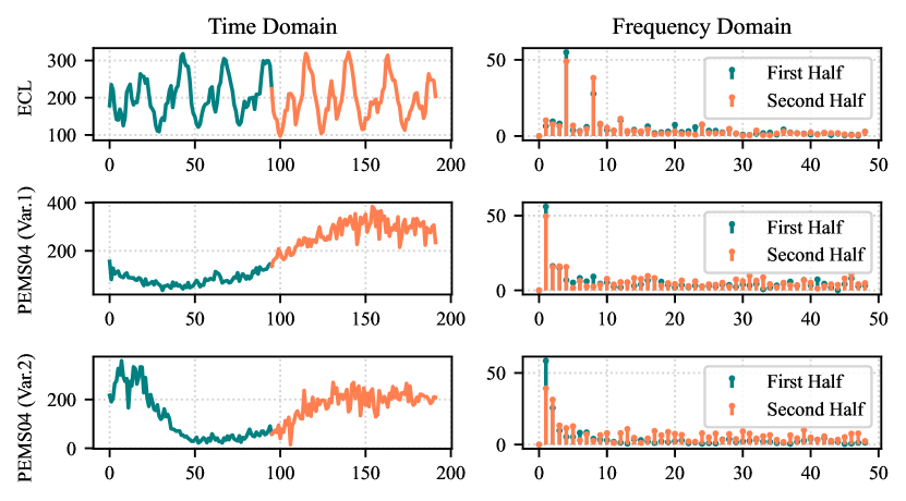
Figure 1: Time series and their corresponding frequency spectra. The series are normalized before applying the DFT, and the amplitudes of the frequency spectra are plotted. (1) The frequency spectra often exhibit strong consistency across adjacent temporal spans within the same time series, forming the basis for frequency-based forecasting. (2) Strong correlations between the two variables in PEMS04 (rows 2 and 3) are observed, suggesting that exploring such multivariate relationships could lead to more robust representations. (3) The frequency spectrum usually exhibits sparsity, with a few dominant frequencies.

In recent years, frequency-domain-based models have been proposed and have achieved great performance Yi et al. (2024c); Xu et al. (2023), benefiting from the robust frequency domain modeling. As shown in Figure 1, frequency spectra exhibit strong consistency across different spans of the same series, making them suitable for forecasting. Most existing frequency-domain-based works Yi et al. (2024a) rely on linear layers to learn frequency-domain representations, resulting in a performance gap. Frequency-domain Transformer-based models remain under-explored. Recently, Fredformer Piao et al. (2024) applies the vanilla Transformer to patched frequency tokens to address the frequency bias issue. However, the patching technique introduces additional hyper-parameters and undermines the inherent global perspective Yi et al. (2024c) of frequency-domain modeling.

In this paper, we adopt a simple yet effective approach by applying the Transformer to frequency-domain variate tokens for representation learning. Specifically, we embed the entire frequency spectrum as variate tokens and capture cross-variate dependencies among them. This architecture offers three main advantages: 1) As shown in Section 3, simple frequency-domain operations can correspond to complex temporal operations Yi et al. (2024c); 2) Inter-variate correlations typically exists (e.g., Figure 1) Liu et al. (2024a), and and learning these correlations could be beneficial for more robust frequency representation; 3) The permutation-invariant nature of the attention mechanism naturally aligns with the order-insensitivity of variates.

Furthermore, we observe that for the frequency-domain representation, the attention matrix of vanilla attention often exhibits a low-rank characteristic, which reduces the diversity of representations. To address this issue, we propose a general solution: adding a learnable matrix to the original softmax attention matrix, followed by row-wise normalization. We term this approach enhanced attention and name the overall model FreEformer. Despite its simplicity, the enhanced attention mechanism is proven effective both theoretically and empirically. The main contributions of this work are summarized as follows:

• This paper presents a simple yet effective model, named FreEformer, for multivariate time series forecasting. FreEformer achieves robust cross-variate representation learning using the enhanced attention mechanism.

• Theoretical analysis and experimental results demonstrate that the enhanced attention mechanism increases the rank of the attention matrix and provides greater flexibility for gradient flow. As a plug-in module, it consistently enhances the performance of existing Transformer-based forecasters.

• Empirically, FreEformer consistently achieves state-of-the-art forecasting performance across 18 real-world benchmarks spanning diverse domains such as electricity, transportation, weather, healthcare and finance.

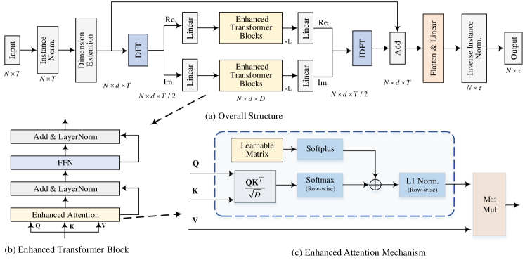
Figure 2: Overall structure of the FreEformer. We leverage the frequency spectrum to capture temporal patterns and employ an enhanced Transformer to model dependencies among multivariate spectra. The enhanced Transformer introduces a learnable matrix to the attention mechanism, which, as shown through theoretical analysis, addresses potential low-rank issues and improves gradient flow.

2 Related Works

2.1 Transformer-Based Forecasters

Classic works such as Autoformer Wu et al. (2021), Informer Zhou et al. (2021), Pyraformer Liu et al. (2022b), FEDformer Zhou et al. (2022b), and PatchTST Nie et al. (2023) represent early Transformer-based time series forecasters. iTransformer Liu et al. (2024a) introduces the inverted Transformer to capture multivariate dependencies, and achieves accurate forecasts. More recently, research has focused on jointly modeling cross-time and cross-variate dependencies Zhang and Yan (2023); Wang et al. (2024c); Han et al. (2024). Leddam Yu et al. (2024) uses a dual-attention module for decomposed seasonal components and linear layers for trend components. Unlike previous models in the time domain, we shift our focus to the frequency domain to explore dependencies among the frequency spectra of multiple variables for more robust representations.

2.2 Frequency-Domain Forecasters

Frequency analysis is an important tool in time series forecasting Yi et al. (2023). FEDformer Zhou et al. (2022b) performs DFT and sampling prior to Transformer. DEPTS Fan et al. (2022) uses the DFT to capture periodic patterns for better forecasts. FiLM Zhou et al. (2022a) applies Fourier analysis to preserve historical information while mitigating noise. FreTS Yi et al. (2024c) employs frequency-domain MLPs to model channel and temporal dependencies. FourierGNN Yi et al. (2024b) transfers GNN operations from the time domain to the frequency domain. FITS Xu et al. (2023) applies a low-pass filter and complex-valued linear projection in the frequency domain. DERITS Fan et al. (2024) introduces a Fourier derivative operator to address non-stationarity. Fredformer Piao et al. (2024) addresses frequency bias by dividing the frequency spectrum into patches. FAN Ye et al. (2024) introduces frequency adaptive normalization for non-stationary data. In this work, we adopt a simple yet effective Transformer-based model to capture multivariate correlations in the frequency domain, outperforming existing methods.

2.3 Transformer Variants

Numerous variants of the vanilla Transformer have been developed to enhance efficiency and performance. Informer Zhou et al. (2021) introduces a ProbSparse self-attention mechanism with $\mathcal{O}(N\mathrm{log}N)$ complexity. Flowformer Wu et al. (2022) proposes Flow-Attention, achieving linear complexity based on flow network theory. Reformer Kitaev et al. (2020) reduces complexity by replacing dot-product attention with locality-sensitive hashing. Linear Transformers, such as FLatten Han et al. (2023) and LSoftmax Yue et al. (2024), achieve linear complexity by precomputing $\mathbf{K}^{T}\mathbf{V}$ and designing various mapping functions. FlashAttention Dao et al. (2022) accelerates computations by tiling to minimize GPU memory operations. LASER Surya Duvvuri and Dhillon (2024) mitigates the gradient vanishing issue using exponential transformations. In this work, we focus on the low-rank issue and adopt a simple yet effective strategy by adding a learnable matrix to the attention matrix. This improves both matrix rank and gradient flow with minimal modifications to the vanilla attention mechanism.

3 Preliminaries

The discrete Fourier transform (DFT) Palani (2022) converts a signal $\mathbf{x}\in\mathbb{R}^{N}$ into its frequency spectrum $\mathcal{F}\in\mathbb{C}^{N}$. For $k=0,1,\cdots,N-1$, we have

$$\mathcal{F}[k]=\sum_{n=0}^{N-1}e^{-j\frac{2\pi}{N}nk}\mathbf{x}[n].$$ (1)

Here, $j$ denotes the imaginary unit. For a real-valued vector $\mathbf{x}$, $\mathcal{F}[k]$ is complex-valued and satisfies the property of Hermitian symmetry Palani (2022): $\mathcal{F}[k]=\left(\mathcal{F}[N-k]\right)^{*}$ for $k=1,\cdots,N-1$, where $\left(\cdot\right)^{*}$ denotes the complex conjugate. The DFT is a linear and reversible transform, with the inverse discrete Fourier transform (IDFT) being:

$$\mathbf{x}[n]=\frac{1}{N}\sum_{k=0}^{N-1}\mathcal{F}[k]\cdot e^{j\cdot 2\pi\frac{k}{N}n},\>k=0,1,\cdots,N-1.$$ (2)

Linear projections in the frequency domain are widely employed in works such as FreTS Yi et al. (2024c) and FITS Xu et al. (2023). The following theorem establishes their equivalent operations in the time domain.

Theorem 1 (Frequency-domain linear projection and time-domain convolutions).

Given the time series $\mathbf{x}\in\mathbb{R}^{N}$ and its corresponding frequency spectrum $\mathcal{F}\in\mathbb{C}^{N}$. Let $\mathbf{W}\in\mathbb{C}^{N\times N}$ denote a weight matrix and $\mathbf{b}\in\mathbb{C}^{N}$ a bias vector. Under these definitions, the following DFT pair holds:

$$\tilde{\mathcal{F}}=\mathbf{W}\mathcal{F}+\mathbf{b}\leftrightarrow\sum_{i=0}^{N-1}{\Omega_{i}\circledast\mathcal{M}_{i}(\mathbf{x})}+\mathrm{IDFT}(\mathbf{b}),$$ (3)

where

$$w_{i}=\left[\mathrm{diag}(\mathbf{W},i),\mathrm{diag}(\mathbf{W},i-N)\right]\in\mathbb{C}^{N},$$ (4)

$$\Omega_{i}=\mathrm{IDFT}\left(w_{i}\right)\in\mathbb{C}^{N},$$

$$\mathcal{M}_{i}(\mathbf{x})=\mathbf{x}\odot\left[\mathrm{e}^{-j\frac{2\pi}{N}ik}\right]_{k=0,1,\cdots N-1}\in\mathbb{C}^{N}.$$

Here, $\circledast$ denotes the circular convolution, and $\odot$ represents the Hadamard (element-wise) product. The notation $\left[\cdot,\cdot\right]$ indicates the concatenation of two vectors. $\mathrm{diag}(\mathbf{W},i)\in\mathbb{C}^{N-\left|i\right|}$ extracts the $i$-th diagonal of $\mathbf{W}$. $\mathcal{M}_{i}(\mathbf{x})$ represents the $i$-th modulated version of $\mathbf{x}$, with $\mathcal{M}_{0}(\mathbf{x})$ being $\mathbf{x}$ itself.

We provide the proof of this theorem in Section A of the appendix. Theorem 1 extends Theorem 2 from FreTS Yi et al. (2024c) and demonstrates that a linear transformation in the frequency domain is equivalent to the sum of circular convolution operations applied to the series and its modulated versions. This equivalence highlights the computational simplicity of performing such operations in the frequency domain compared to the time domain.

4 Method

In multivariate time series forecasting, we consider historical series within a lookback window of $T$, each timestamp with $N$ variates: $\mathbf{x}=\left\{\mathrm{x}_{1},\cdots,\mathrm{x}_{T}\right\}\in\mathbb{R}^{N\times T}$. Our task is to predict future $\tau$ timestamps to closely approximate the ground truth $\mathbf{y}=\left\{\mathrm{x}_{T+1},\cdots,\mathrm{x}_{T+\tau}\right\}\in\mathbb{R}^{N\times\tau}$.

4.1 Overall Architecture

As shown in Figure 2, FreEformer employs a simple architecture. First, an instance normalization layer, specifically RevIN Kim et al. (2021), is used to normalize the input data and de-normalize the results at the final stage to mitigate non-stationarity. The constant mean component, represented by the zero-frequency point in the frequency domain, is set to zero during normalization. Subsequently, a dimension extension module is employed to enhance the model’s representation capabilities. Specifically, the input $\mathbf{x}$ is expanded by a learnable weight vector $\phi_{d}\in\mathbb{R}^{d}$, yielding higher-dimensional and more expressive series data: $\bar{\mathbf{x}}=\mathbf{x}\times\phi_{d}\in\mathbb{R}^{N\times d\times T}$. We refer to $d$ as the embedding dimension.

Frequency-Domain Operations

Next, we apply the Discrete Fourier Transform (DFT) to convert the time series $\bar{\mathbf{x}}$ into its frequency spectrum along the temporal dimension:

$$\mathcal{F}=\mathrm{DFT}(\bar{\mathbf{x}})=\mathrm{Re}(\mathcal{F})+j\cdot\mathrm{Im}(\mathcal{F})\in\mathbb{C}^{N\times d\times T},$$ (5)

where $\mathrm{Re}(\cdot)$ and $\mathrm{Im}(\cdot)$ represent the real and imaginary parts, respectively. Due to the conjugate symmetry property of the frequency spectrum of a real-valued signal, only the first $\left\lceil(T+1)/2\right\rceil$ elements of the real and imaginary parts need to be retained. Here, $\left\lceil\cdot\right\rceil$ denotes the ceiling operation.

Dataset	ECL	Weather	Traffic	COVID-19	NASDAQ	COVID-19	NASDAQ
$T-\tau$	96-{96,192,336,720}			36-{24,36,48,60}		12-{3,6,9,12}
Concat.	0.162	0.243	0.443	8.705	0.190	1.928	0.055
S.W.	0.165	0.240	0.440	8.520	0.189	1.895	0.055
N.S.W.	0.162	0.239	0.435	8.435	0.185	1.892	0.055

Table 1: Comparison of different processes for real and imaginary parts. Average MSEs are reported in this table. ‘S.W.’ and ‘N.S.W.’ denote ‘Shared Weights’ and ‘Non-Shared Weights’, respectively. ‘Concat.’ denotes the concatenation method.

To process the real and imaginary parts, common strategies include employing complex-valued layers Yi et al. (2024c); Xu et al. (2023), or concatenating the real and imaginary parts into a real-valued vector and subsequently projecting the results back Piao et al. (2024). In this work, we adopt a simple yet effective scheme: processing these two parts independently. As shown in Table 1, this independent processing scheme yields better performance for FreEformer.

After flattening the last two dimensions of the real and imaginary parts and projecting them into the hidden dimension $D$, we construct the frequency-domain variate tokens $\tilde{\mathrm{Re}},\tilde{\mathrm{Im}}\in\mathbb{R}^{N\times D}$. These tokens are then fed into $L$ stacked Transformer blocks to capture multivariate dependencies among the spectra. Subsequently, the tokens are projected back to the lookback length. The real and imaginary parts are then regrouped to reconstruct the frequency spectrum. Then, the time-domain signal $\tilde{\mathbf{x}}$ is recovered using the IDFT. The entire process is summarized as follows:

$$\tilde{\mathcal{F}}=\mathcal{F}[:,:,0:\left\lceil(T+1)/2\right\rceil]\in\mathbb{C}^{N\times d\times\left\lceil(T+1)/2\right\rceil},$$ (6)

$$\tilde{\mathrm{Re}}^{0}=\mathrm{Linear}(\mathrm{Flatten}(\mathrm{Re}(\tilde{\mathcal{F}})))\in\mathbb{R}^{N\times D}$$

$$\tilde{\mathrm{Re}}^{l+1}=\mathrm{TrmBlock}(\tilde{\mathrm{Re}}^{l})\in\mathbb{R}^{N\times D},l=0,\cdots,L-1,$$

$$\tilde{\mathrm{Re}}=\mathrm{Linear}(\mathrm{Reshape}(\tilde{\mathrm{Re}}^{L}))\in\mathbb{R}^{N\times d\times\left\lceil(T+1)/2\right\rceil},$$

$$\tilde{\mathrm{Im}}^{0}=\mathrm{Linear}(\mathrm{Flatten}(\mathrm{Im}(\tilde{\mathcal{F}})))\in\mathbb{R}^{N\times D}$$

$$\tilde{\mathrm{Im}}^{l+1}=\mathrm{TrmBlock}(\tilde{\mathrm{Im}}^{l})\in\mathbb{R}^{N\times D},l=0,\cdots,L-1,$$

$$\tilde{\mathrm{Im}}=\mathrm{Linear}(\mathrm{Reshape}(\tilde{\mathrm{Im}}^{L}))\in\mathbb{R}^{N\times d\times\left\lceil(T+1)/2\right\rceil},$$

$$\tilde{\mathbf{x}}=\mathrm{IDFT}(\tilde{\mathrm{Re}}+j\cdot\tilde{\mathrm{Im}})\in\mathbb{R}^{N\times d\times T}.$$

In the above equation, the final step is implemented via the irfft function in PyTorch to ensure real-valued outputs.

Prediction Head

A shortcut connection is applied to sum $\tilde{\mathbf{x}}$ with the original $\bar{\mathbf{x}}$. Finally, a flatten layer and a linear head are used to ensure the output matches the desired size. The final result is obtained through a de-normalization step:

$$\mathbf{\hat{y}}=\mathrm{DeNorm}\left(\mathrm{Linear}(\mathrm{Flatten}(\tilde{\mathbf{x}}+\bar{\mathbf{x}}))\right)\in\mathbb{R}^{N\times\tau}.$$ (7)

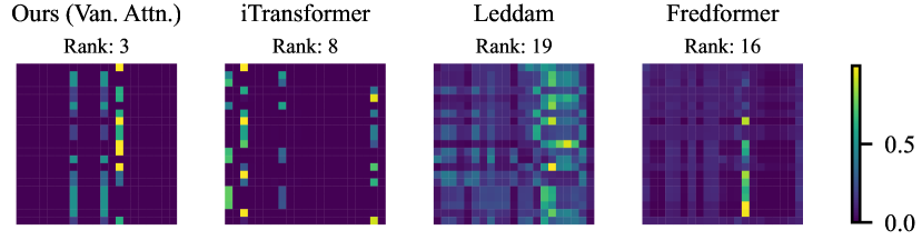
Figure 3: Attention matrices from state-of-the-art forecasters on the Weather dataset. The FreEformer with vanilla attention typically exhibits a low rank, likely due to the inherent sparsity of the frequency spectrum and the strong-value-focused nature of the Softmax function in vanilla attention.

4.2 Enhanced Attention

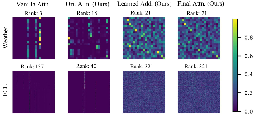
Figure 4: Attention matrices from vanilla and enhanced attention. The left column shows the low-rank attention matrix from the vanilla attention (Weather: 3, ECL: 137), with most entries near zero. The right three columns show the original attention matrix ($\mathbf{A}$), the learned addition matrix ($\mathrm{Softplus}(\mathbf{B})$), and the final attention matrix ($\mathrm{Norm}\left(\mathbf{A}+\mathrm{Softplus}(\mathbf{B})\right)$). The final matrix exhibits more prominent values and higher ranks (Weather: 21, ECL: 321).

In the Transformer block, as shown in Figure 2(b), we first employ the attention mechanism to capture cross-variate dependencies. Then the LayerNorm and FFN are used to update frequency representations in a variate-independent manner. According to Theorem 1, the FFN corresponds to a series of convolution operations in the time domain for series representations. The vanilla attention mechanism is defined as:

$$\mathrm{Attn}\left(\mathbf{Q},\mathbf{K},\mathbf{V}\right)=\underbrace{\mathrm{Softmax}\left(\frac{\mathbf{Q}\mathbf{K}^{T}}{\sqrt{D}}\right)}_{\text{Attention Matrix}\triangleq\mathbf{A}}\mathbf{V}.$$ (8)

Here, $\mathbf{Q},\mathbf{K},\mathbf{V}\in\mathbb{R}^{N\times D}$ are the query, key and value matrix, respectively, obtained through linear projections. We denote $D$ as the feature dimension and refer to $\mathrm{Softmax}\left(\mathbf{Q}\mathbf{K}^{T}/\sqrt{D}\right)$, represented as $\mathbf{A}$, as the attention matrix.

However, as shown in Figure 3, compared to other state-of-the-art forecasters, FreEformer with the vanilla attention mechanism usually exhibits an attention matrix with a lower rank. This could arise from the inherent sparsity of the frequency spectrum Palani (2022) and the strong-value-focused properties of the vanilla attention mechanism Surya Duvvuri and Dhillon (2024); Xiong et al. (2021). While patching adjacent frequency points can mitigate sparsity (as in Fredformer), we address the underlying low-rank issue within the attention mechanism itself, offering a more general solution.

In this work, we adopt a straightforward yet effective solution: introducing a learnable matrix $\mathbf{B}$ to the attention matrix. The enhanced attention mechanism, denoted as $\mathrm{EnhAttn}\left(\mathbf{Q},\mathbf{K},\mathbf{V}\right)$, is defined as :

$$\mathrm{Norm}\left(\mathrm{Softmax}\left(\frac{\mathbf{Q}\mathbf{K}^{T}}{\sqrt{D}}\right)+\mathrm{Softplus}(\mathbf{B})\right)\mathbf{V},$$ (9)

where $\mathrm{Norm}(\cdot)$ denotes row-wise L1 normalization. The $\mathrm{Softplus}(\cdot)$ function ensures positive entries, thereby preventing potential division-by-zero errors in $\mathrm{Norm}(\cdot)$.

4.2.1 Theoretical Analysis

Feature Diversity

According to Equation (9), feature diversity is directly influenced by the rank of the final attention matrix $\mathrm{Norm}\left(\mathbf{A}+\bar{\mathbf{B}}\right)$, where $\bar{\mathbf{B}}\triangleq\mathrm{Softplus}(\mathbf{B})$. Since row-wise L1 normalization does not alter the rank of a matrix, we have: $\mathrm{rank}\left(\mathrm{Norm}\left(\mathbf{A}+\bar{\mathbf{B}}\right)\right)=\mathrm{rank}\left(\mathbf{A}+\bar{\mathbf{B}}\right)$. For further analysis, we present the following theorem:

Theorem 2.

Let $\mathbf{A}$ and $\mathbf{B}$ be two matrices of the same size $N\times N$. The rank of their sum satisfies the following bounds:

$$\left|\mathrm{rank}(\mathbf{A})-\mathrm{rank}(\mathbf{B})\right|\leq\mathrm{rank}(\mathbf{A}+\mathbf{B})\leq\mathrm{rank}(\mathbf{A})+\mathrm{rank}(\mathbf{B})$$ (10)

The proof is provided in Section B of the appendix. As illustrated in Figure 4, the original attention matrix $\mathbf{A}$ often exhibits a low rank, whereas the learned matrix $\bar{\mathbf{B}}$ is nearly full-rank. According to Theorem 2, the combined matrix $\mathbf{A}+\bar{\mathbf{B}}$ generally achieves a higher rank. This observation aligns with the results shown in Figure 4.

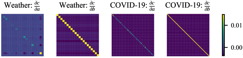
Figure 5: Illustration of the Jacobian matrices of $\mathbf{c}$ with respect to $\mathbf{a}$ and $\mathbf{b}$ for the Weather and COVID-19 datasets.

Gradient Flow

Let $\mathbf{a}\in\mathbb{R}^{N}$ denote a row in $\mathbf{Q}\mathbf{K}^{T}/\sqrt{D}$. For vanilla attention, the transformation is $\tilde{\mathbf{a}}\triangleq\mathrm{Softmax}(\mathbf{a})$. Then the Jacobian matrix of $\tilde{\mathbf{a}}$ regarding $\mathbf{a}$ can be derived as:

$$\frac{\partial\tilde{\mathbf{a}}}{\partial\mathbf{a}}=\mathrm{Diag}(\tilde{\mathbf{a}})-\tilde{\mathbf{a}}\tilde{\mathbf{a}}^{T},$$ (11)

where $\mathrm{Diag}(\tilde{\mathbf{a}})$ is a diagonal matrix with $\tilde{\mathbf{a}}$ as its diagonal.

For the enhanced attention, the transformation is given by:

$$\mathbf{c}=\mathrm{Norm}\left(\mathrm{Softmax}(\mathbf{a})+\mathbf{b}\right),$$ (12)

where $\mathbf{b}$ represents a row of $\mathrm{Softplus}(\mathbf{B})$. The Jacobian matrices of $\mathbf{c}$ with respect to $\mathbf{a}$ and $\mathbf{b}$ can be derived as:

$$\frac{\partial\mathbf{c}}{\partial\mathbf{a}} =\frac{1}{\left\|\tilde{\mathbf{b}}\right\|_{1}}\left(\mathrm{Diag}(\tilde{\mathbf{a}})-\tilde{\mathbf{a}}\tilde{\mathbf{a}}^{T}\right),$$ (13)

$$\frac{\partial\mathbf{c}}{\partial\mathbf{b}} =\frac{1}{\left\|\tilde{\mathbf{b}}\right\|_{1}^{2}}\left(\left\|\tilde{\mathbf{b}}\right\|_{1}\cdot\mathbf{I}-\tilde{\mathbf{b}}\mathbf{1}^{T}\right),$$

where $\tilde{\mathbf{b}}=\tilde{\mathbf{a}}+\mathbf{b}=\mathrm{Softmax}(\mathbf{a})+\mathbf{b}$, $\mathbf{I}\in\mathbb{R}^{N\times N}$ is the unit matrix; $\mathbf{1}=\left[1,\cdots,1\right]^{T}\in\mathbb{R}^{N}$. The detailed proofs of Equations (11) and (13) are provided in Section C of the appendix.

We can see that $\partial\mathbf{c}/\partial\mathbf{a}$ in Equation (13) shares the same structure as that of vanilla attention in Equation (11), except for the scaling factor $1/\left|\tilde{\mathbf{b}}\right|_{1}$. Since $\left\|\tilde{\mathbf{b}}\right\|_{1}=1+\left\|\mathbf{b}\right\|_{1}>1$ and $\tilde{\mathbf{b}}$ is learnable, the gradient is scaled down by a learnable factor, providing extra flexibility in gradient control.

Moreover, as shown in Figure 5, $\partial\mathbf{c}/\partial\mathbf{b}$ exhibits a pronounced diagonal than $\partial\mathbf{c}/\partial\mathbf{a}$, suggesting a stronger dependence of $\mathbf{c}$ on $\mathbf{b}$ than $\mathbf{a}$. This aligns with the design, as $\mathbf{b}$ directly modulates the attention weights.

Combination of MLP and Vanilla Attention

We now provide a new perspective on the enhanced attention. In Equation (9), the attention matrix is decomposed into two components: the input-independent, dataset-specific term $\bar{\mathbf{B}}$, and the input-dependent term $\mathbf{A}$. If $\mathbf{A}$ is zero, the enhanced attention reduces to a linear transformation of $\mathbf{V}$, effectively functioning as an MLP along the variate dimension. By jointly optimizing $\mathbf{A}$ and $\bar{\mathbf{B}}$, the enhanced attention can be interpreted as an adaptive combination of MLP and vanilla attention.

5 Experiments

Datasets and Implementation Details

We extensively evaluate the FreEformer using eighteen real-world datasets: ETT (four subsets), Weather, ECL, Traffic, Exchange, Solar-Energy, PEMS (four subsets), ILI, COVID-19, ECG, METR-LA, NASDAQ and Wiki. During training, we adopt the L1 loss function from CARD Wang et al. (2024c). The embedding dimension $d$ is fixed at 16, and the dimension $D$ is selected from $\left\{128,256,512\right\}$. The dataset description and implementation details are provided in the appendix.

5.1 Forecasting Performance

Model	FreEformer (Ours)		Leddam Yu et al. (2024)		CARD Wang et al. (2024c)		Fredformer Wang et al. (2024a)		iTrans. Liu et al. (2024a)		TimeMixer Wang et al. (2024b)		PatchTST Nie et al. (2023)		Crossfm. Zhang and Yan (2023)		TimesNet Wu et al. (2023a)		FreTS Yi et al. (2024c)		DLinear Zeng et al. (2023)
Metric	MSE	MAE	MSE	MAE	MSE	MAE	MSE	MAE	MSE	MAE	MSE	MAE	MSE	MAE	MSE	MAE	MSE	MAE	MSE	MAE	MSE	MAE
ETTm1	0.379	0.381	0.386	0.397	0.383	0.384	0.384	0.395	0.407	0.410	0.381	0.395	0.387	0.400	0.513	0.496	0.400	0.406	0.407	0.415	0.403	0.407
ETTm2	0.272	0.313	0.281	0.325	0.272	0.317	0.279	0.324	0.288	0.332	0.275	0.323	0.281	0.326	0.757	0.610	0.291	0.333	0.335	0.379	0.350	0.401
ETTh1	0.433	0.431	0.431	0.429	0.442	0.429	0.435	0.426	0.454	0.447	0.447	0.440	0.469	0.454	0.529	0.522	0.458	0.450	0.488	0.474	0.456	0.452
ETTh2	0.372	0.393	0.373	0.399	0.368	0.390	0.365	0.393	0.383	0.407	0.364	0.395	0.384	0.405	0.942	0.684	0.414	0.427	0.550	0.515	0.559	0.515
ECL	0.162	0.251	0.169	0.263	0.168	0.258	0.176	0.269	0.178	0.270	0.182	0.272	0.208	0.295	0.244	0.334	0.192	0.295	0.202	0.290	0.212	0.300
Exchange	0.354	0.399	0.354	0.402	0.362	0.402	0.333	0.391	0.360	0.403	0.387	0.416	0.367	0.404	0.940	0.707	0.416	0.443	0.416	0.439	0.354	0.414
Traffic	0.435	0.251	0.467	0.294	0.453	0.282	0.433	0.291	0.428	0.282	0.484	0.297	0.531	0.343	0.550	0.304	0.620	0.336	0.538	0.328	0.625	0.383
Weather	0.239	0.260	0.242	0.272	0.239	0.265	0.246	0.272	0.258	0.279	0.240	0.271	0.259	0.281	0.259	0.315	0.259	0.287	0.255	0.298	0.265	0.317
Solar	0.217	0.219	0.230	0.264	0.237	0.237	0.226	0.262	0.233	0.262	0.216	0.280	0.270	0.307	0.641	0.639	0.301	0.319	0.226	0.254	0.330	0.401
PEMS03	0.102	0.206	0.107	0.210	0.174	0.275	0.135	0.243	0.113	0.221	0.167	0.267	0.180	0.291	0.169	0.281	0.147	0.248	0.169	0.278	0.278	0.375
PEMS04	0.094	0.196	0.103	0.210	0.206	0.299	0.162	0.261	0.111	0.221	0.185	0.287	0.195	0.307	0.209	0.314	0.129	0.241	0.188	0.294	0.295	0.388
PEMS07	0.080	0.167	0.084	0.180	0.149	0.247	0.121	0.222	0.101	0.204	0.181	0.271	0.211	0.303	0.235	0.315	0.124	0.225	0.185	0.282	0.329	0.395
PEMS08	0.110	0.194	0.122	0.211	0.201	0.280	0.161	0.250	0.150	0.226	0.226	0.299	0.280	0.321	0.268	0.307	0.193	0.271	0.212	0.297	0.379	0.416

Table 2: Long-term time series forecasting results for $T=96$ and $\tau\in\left\{96,192,336,720\right\}$. For PEMS, $\tau\in\left\{12,24,48,96\right\}$. Results are averaged across these prediction lengths. These settings are used throughout the following tables.

Model		FreEformer (Ours)		Leddam Yu et al. (2024)		CARD Wang et al. (2024c)		Fredformer Wang et al. (2024a)		iTrans. Liu et al. (2024a)		TimeMixer Wang et al. (2024b)		PatchTST Nie et al. (2023)		TimesNet Wu et al. (2023a)		DLinear Zeng et al. (2023)		FreTS Yi et al. (2024c)
Metric		MSE	MAE	MSE	MAE	MSE	MAE	MSE	MAE	MSE	MAE	MSE	MAE	MSE	MAE	MSE	MAE	MSE	MAE	MSE	MAE
	S1	1.140	0.585	1.468	0.679	1.658	0.707	1.518	0.696	1.437	0.659	1.707	0.734	1.681	0.723	1.480	0.684	2.400	1.034	1.839	0.782
ILI	S2	1.906	0.835	1.982	0.875	2.260	0.938	1.947	0.899	1.993	0.887	2.020	0.878	2.128	0.885	2.139	0.931	3.083	1.217	3.036	1.174
	S1	1.892	0.673	2.064	0.779	2.059	0.767	1.902	0.765	2.096	0.795	2.234	0.782	2.221	0.820	2.569	0.861	3.483	1.102	2.516	0.862
COVID-19	S2	8.435	1.764	8.439	1.792	9.013	1.862	8.656	1.808	8.506	1.792	9.604	1.918	9.451	1.905	9.644	1.877	13.075	2.099	11.345	1.958
	S1	0.336	0.221	0.327	0.243	0.349	0.233	0.336	0.242	0.338	0.244	0.334	0.245	0.335	0.243	0.344	0.253	0.341	0.294	0.324	0.279
METR-LA	S2	0.840	0.406	0.878	0.490	0.929	0.466	0.898	0.495	0.916	0.501	0.881	0.499	0.893	0.502	0.890	0.488	0.819	0.550	0.804	0.543
	S1	0.055	0.126	0.059	0.135	0.057	0.130	0.059	0.135	0.060	0.137	0.055	0.126	0.058	0.132	0.068	0.151	0.072	0.170	0.080	0.184
NASDAQ	S2	0.185	0.277	0.196	0.286	0.193	0.284	0.194	0.285	0.207	0.297	0.186	0.281	0.198	0.286	0.255	0.343	0.228	0.331	0.263	0.361
	S1	6.524	0.391	6.547	0.404	6.553	0.400	6.705	0.406	6.569	0.405	6.572	0.409	6.523	0.404	7.956	0.520	6.634	0.481	6.521	0.448
Wiki	S2	6.259	0.442	6.286	0.463	6.285	0.453	5.931	0.453	6.275	0.458	6.315	0.468	6.212	0.444	7.310	0.623	6.205	0.539	6.147	0.505

Table 3: Short-term time series forecasting results under two settings: S1 (Input-12, Predict-$\left\{3,6,9,12\right\}$) and S2 (Input-36, Predict-$\left\{24,36,48,60\right\}$). Average results are reported across four prediction lengths. S1 is the default setting in the following experiments.

We choose 10 well-acknowledged deep forecasters as our baselines, including (1) Transformer-based models: Leddam Yu et al. (2024), CARD Wang et al. (2024c), Fredformer Piao et al. (2024), iTransformer Liu et al. (2024a), PatchTST Nie et al. (2023), Crossformer Zhang and Yan (2023); (2) Linear-based models: TimeMixer Wang et al. (2024b), FreTS Yi et al. (2024c) and DLinear Zeng et al. (2023); (3) TCN-based model: TimesNet Wu et al. (2023a).

Comprehensive results for long- and short-term forecasting are presented in Tables 2 and 3, respectively, with the best results highlighted in bold and the second-best underlined. FreEformer consistently outperforms state-of-the-art models across various prediction lengths and real-world domains. Compared with sophisticated time-domain-based models, such as Leddam and CARD, FreEformer achieves superior performance with a simpler architecture, benefiting from the global-level property of the frequency domain. Furthermore, its performance advantage over Fredformer, another Transformer- and frequency-based model, suggests that the deliberate patching of band-limited frequency spectra may introduce unnecessary noise, hindering forecasting accuracy.

Notably, in Table 4, we compare FreEformer with additional frequency-based models, where it also demonstrates a clear performance advantage. The visualization results of FreEformer are presented in Figure 6. Furthermore, as shown in Table 10 of the appendix, FreEformer exhibits state-of-the-art performance with variable lookback lengths.

Models	FreEformer (Ours)		FITS Xu et al. (2023)		FAN Ye et al. (2024)		FilterNet Yi et al. (2024a)		FreDF Wang et al. (2024a)
Metric	MSE	MAE	MSE	MAE	MSE	MAE	MSE	MAE	MSE	MAE
ETT(Avg)	0.364	0.380	0.408	0.405	0.405	0.427	0.367	0.384	0.369	0.384
ECL	0.162	0.251	0.384	0.434	0.208	0.298	0.201	0.285	0.170	0.259
Traffic	0.435	0.251	0.615	0.370	0.526	0.357	0.521	0.340	0.421	0.279
Weather	0.239	0.260	0.273	0.292	0.247	0.292	0.248	0.274	0.254	0.274

Table 4: Comparison with additional state-of-the-art frequency-based models. Average results are reported across four prediction lengths. ‘Avg’ refers to averages further computed over subsets.

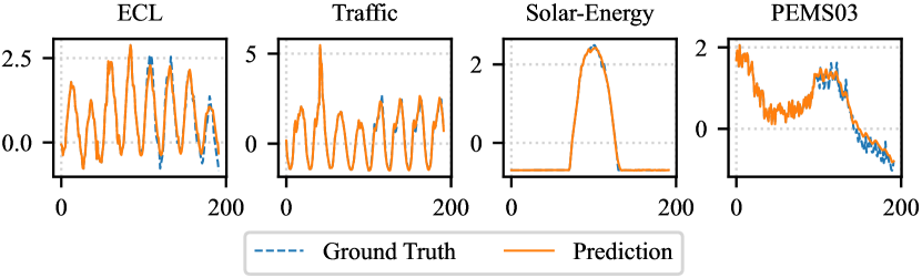
Figure 6: Visualization of the forecasting results under the ‘Input-96-Predict-96’ setting, demonstrating accurate approximations.

5.2 Model Analysis

Layer	Dim.	Patch.	ETTm1	Weather	ECL	Traffic	COVID-19
Linear	Var.	✗	0.385	0.245	0.189	0.488	2.040
Linear	Fre.	✗	0.386	0.246	0.184	0.482	2.086
Trans.	Fre.	✔	0.381	0.244	0.183	0.504	2.100
Trans.	Fre.	✗	0.383	0.245	0.181	0.489	2.116
Trans.	Var.	✔	0.385	0.241	0.162	0.443	2.029
Trans.	Var.	✗	0.379	0.239	0.162	0.435	1.892

Table 5: Architecture ablations on layers, dimensions, and patching settings. Layers include linear and enhanced Transformer layers, while dimensions refer to frequency and variate dimensions. ‘Patch.’ indicates patching along the frequency dimension, with patch length and stride set to 6 and 3 for COVID-19, and 16 and 8 for other datasets. Average MSEs are reported across four prediction horizons. The final row corresponds to the FreEformer configuration.

Architecture Ablations

The FreEformer utilizes an enhanced Transformer architecture to capture cross-variate dependencies in the frequency domain. Table 5 presents a comparison of several FreEformer variants, evaluating the impact of linear and enhanced Transformer layers, different dimensional configurations, and patching along the frequency dimension. To ensure a fair comparison, the enhanced Transformer is used for all Transformer-based settings. The results indicate that: 1) Enhanced Transformer blocks outperform linear layers due to their superior representation capabilities; 2) Multivariate dependency learning generally outperforms inter-frequency learning, aligning with the claim in FreDF Wang et al. (2024a) that correlations among frequency points are minimal; 3) Furthermore, patching does not improve FreEformer, likely because patching frequencies creates localized receptive fields, thereby limiting access to global information.

Attn.	Domain	Traffic	PEMS03	Weather	Solar	ILI
Ours	Fre.	0.435	0.102	0.239	0.217	1.140
	Time	0.443	0.122	0.243	0.228	1.375
Vanilla	Fre.	0.451	0.113	0.245	0.220	1.510
	Time	0.441	0.146	0.248	0.226	2.140

Table 6: Performance comparison of the frequency-domain and time-domain representation learning under two attention settings. Average MSEs are reported across four prediction lengths.

Frequency-Domain vs. Temporal Representation

To construct the time-domain variant of FreEformer, we remove the DFT and IDFT steps, as well as the imaginary branch. As shown in Table 6, the frequency-domain representation achieves an average improvement of 8.4% and 10.7% in MSE compared to the time-domain version under the enhanced and vanilla attention settings, respectively. Additionally, we show in Section I.1 of the appendix that Fourier bases generally outperform Wavelet and polynomial bases for our model.

Head	ETTm1	Weather	ECL	Traffic	Solar	NASDAQ	COVID-19
Fre.	0.379	0.245	0.160	0.441	0.216	0.055	1.930
Time	0.379	0.239	0.162	0.435	0.217	0.055	1.892

Table 7: Performance comparison of frequency-domain and temporal prediction heads. Average MSEs are reported.

Prediction Head

In our model, after performing frequency domain representation learning, we apply a temporal prediction head to generate the final predictions. In contrast, some frequency-based forecasters (e.g., FITS and Fredformer) directly predict the future frequency spectrum and transform it back to the time domain as the final step. In FreEformer, the frequency prediction head is formulated as:

$$\mathbf{\hat{y}}=\mathrm{DeNorm}\left(\mathrm{IDFT}\left(\mathrm{FlatLin}(\tilde{\mathrm{Re}})+j\cdot\mathrm{FlatLin}(\tilde{\mathrm{Im}})\right)\right),$$ (14)

where $\tilde{\mathrm{Re}}$ and $\tilde{\mathrm{Im}}$ are defined in Equation (6). As shown in Table 7, the temporal head slightly outperforms the frequency-domain head, highlighting the challenges of accurately forecasting the frequency spectrum. Additionally, Equation (14) incurs higher computational costs in the IDFT step when $\tau>T$, as in long-term forecasting scenarios.

5.3 Enhanced Attention Analysis

Dataset	Ours	Trans. Vaswani et al. (2017)	Flowfm. Wu et al. (2022)	Flashfm. Dao et al. (2022)	Flatten Han et al. (2023)	Mamba Gu and Dao (2023)	LASER Surya Duvvuri and Dhillon (2024)	Lin.Attn. Yue et al. (2024)
Traffic	0.435	0.451	0.453	0.448	0.453	0.443	0.451	0.452
PEMS03	0.102	0.113	0.113	0.114	0.114	0.115	0.111	0.115
Weather	0.239	0.245	0.242	0.245	0.248	0.243	0.244	0.245
Solar	0.217	0.220	0.224	0.221	0.229	0.228	0.219	0.230
ILI	1.140	1.510	1.288	1.547	1.842	1.508	1.596	1.453

Table 8: Comparison of the enhanced Transformer with state-of-the-art attention models and Mamba. Average MSEs are reported across four prediction lengths. Results outperforming state-of-the-art forecasters Leddam and CARD are highlighted in red.

We compare the enhanced Transformer with vanilla Transformer, state-of-the-art Transformer variants and Mamba Gu and Dao (2023) in Table 8. The enhanced Transformer consistently outperforms other models, verifying the effectiveness of the enhanced attention mechanism.

Dataset	iTrans.		PatchTST		Leddam		Fredformer
	Van.	E.A.	Van.	E.A.	Van.	E.A.	Van.	E.A.
ETTm1	0.407	0.389	0.387	0.381	0.386	0.384	0.384	0.385
ECL	0.178	0.165	0.208	0.181	0.169	0.167	0.176	0.169
PEMS07	0.101	0.086	0.211	0.156	0.084	0.080	0.121	0.103
Solar	0.233	0.226	0.270	0.232	0.230	0.228	0.226	0.222
Weather	0.258	0.249	0.259	0.245	0.242	0.242	0.246	0.242
METR-LA	0.338	0.329	0.335	0.335	0.327	0.321	0.336	0.334

Table 9: Comparison of state-of-the-art models using vanilla (Van.) and enhanced attention (E.A.). Only the attention mechanism is updated, with other components and the loss function kept unchanged. Average MSEs across four prediction lengths are reported.

We further apply the enhanced attention mechanism to state-of-the-art forecasters, as shown in Table 9. This yields average MSE improvements of 5.9% for iTransformer, 9.9% for PatchTST, 1.4% for Leddam (with updates only to the ‘cross-channel attention’ module), and 3.8% for FreEformer. These results demonstrate the versatility and effectiveness of the enhanced attention mechanism. Moreover, comparing Tables 2 and 9, FreEformer consistently outperforms these improved forecasters, underscoring its architectural advantages.

In the appendix, we further demonstrate FreEformer’s performance superiority on more metrics (e.g., MASE, correlation coefficient). Remarkably, FreEformer, trained from scratch, achieves superior or comparable performance to a pre-trained model fine-tuned on the same training data.

6 Conclusion

In this work, we present a simple yet effective multivariate time series forecasting model based on a frequency-domain enhanced Transformer. The enhanced attention mechanism is demonstrated to be effective both theoretically and empirically. It can consistently bring performance improvements for state-of-the-art Transformer-based forecasters. We hope that FreEformer will serve as a strong baseline for the time series forecasting community.

Appendix A Theorem 1 and Its Proof

Theorem 3 (Frequency-domain linear projection and time-domain convolutions).

Given the time series $\mathbf{x}\in\mathbb{R}^{N}$ and its corresponding frequency spectrum $\mathcal{F}\in\mathbb{C}^{N}$. Let $\mathbf{W}\in\mathbb{C}^{N\times N}$ denote a weight matrix and $\mathbf{b}\in\mathbb{C}^{N}$ a bias vector. Under these definitions, the following DFT pair holds:

$$\tilde{\mathcal{F}}=\mathbf{W}\mathcal{F}+\mathbf{b}\leftrightarrow\sum_{i=0}^{N-1}{\Omega_{i}\circledast\mathcal{M}_{i}(\mathbf{x})}+\mathrm{IDFT}(\mathbf{b}),$$ (15)

where

$$w_{i}=\left[\mathrm{diag}(\mathbf{W},i),\mathrm{diag}(\mathbf{W},i-N)\right]\in\mathbb{C}^{N},$$ (16)

$$\Omega_{i}=\mathrm{IDFT}\left(w_{i}\right)\in\mathbb{C}^{N},$$

$$\mathcal{M}_{i}(\mathbf{x})=\mathbf{x}\odot\left[\mathrm{e}^{-j\frac{2\pi}{N}ik}\right]_{k=0,1,\cdots N-1}\in\mathbb{C}^{N}.$$

Here, $j$ is the imaginary unit, $\leftrightarrow$ denotes the DFT pair relationship, $\circledast$ represents the circular convolution, $\odot$ indicates the Hadamard (element-wise) product, and $\left[\cdot,\cdot\right]$ represents the concatenation of two vectors. $\mathrm{diag}(\mathbf{W},i)\in\mathbb{C}^{N-\left|i\right|}$ extracts the $i$-th diagonal of $\mathbf{W}$, and $\mathrm{diag}(\mathbf{W},N)$ is defined as $\emptyset$. If $i=0$, $\mathrm{diag}(\mathbf{W},i)$ corresponds to the main diagonal; if $i>0$ (or $i<0$), it corresponds to a diagonal above (or below) the main diagonal. $\mathcal{M}_{i}(\mathbf{x})$ represents the $i$-th modulated version of $\mathbf{x}$, with $\mathcal{M}_{0}(\mathbf{x})$ being $\mathbf{x}$ itself.

Proof.

To prove Theorem 1, we first introduce two supporting lemmas.

1) A circular shift in the frequency domain corresponds to a multiplication by a complex exponential in the time domain. This can be expressed as follows:

$$\mathrm{Roll}(\mathcal{F},-k)\leftrightarrow\mathbf{x}\odot\left[\mathrm{e}^{-j\frac{2\pi}{N}nk}\right]_{n=0,1,\cdots N-1},$$ (17)

where $\mathrm{Roll}(\mathcal{F},-k)$ denotes a circular shift of $\mathcal{F}$ to the left by $k$ elements, e.g., $\mathrm{Roll}(\mathcal{F},-1)=[f_{2},\cdots,f_{N},f_{1}]^{T}$.

2) Multiplication in the frequency domain corresponds to convolution in the time domain. If $\mathcal{F}_{1}\leftrightarrow\mathbf{x}_{1}$ and $\mathcal{F}_{2}\leftrightarrow\mathbf{x}_{2}$, we have

$$\mathcal{F}_{1}\odot\mathcal{F}_{2}\leftrightarrow\mathbf{x}_{1}\circledast\mathbf{x}_{2}.$$ (18)

The proof of Equations (17) and (18) can be found in the literature Palani [2022]; Lu [1989].

Now we analyze the matrix multiplication $\mathbf{W}\mathcal{F}$. Let $\mathrm{DiagMat}(\mathbf{W},(i,i-N))$ denote the matrix that retains only the specified two diagonals of $\mathbf{W}$ while setting all other elements to zero. Using this notation, the matrix $\mathbf{W}$ can be expressed as:

$$\mathbf{W}=\mathrm{DiagMat}(\mathbf{W},0)+\sum_{i=1}^{N-1}\mathrm{DiagMat}\left(\mathbf{W},(i,i-N)\right).$$ (19)

Considering the definition of $w_{i}$ in Equation (16), we have

$$\mathrm{DiagMat}(\mathbf{W},0)\mathcal{F}=\mathrm{diag}(\mathbf{W},0)\odot\mathcal{F}=w_{0}\odot\mathrm{Roll}(\mathcal{F},0),$$ (20)

$$\mathrm{DiagMat}(\mathbf{W},(i,i-N))\mathcal{F}=w_{i}\odot\mathrm{Roll}(\mathcal{F},-i).$$

By combining these results, $\tilde{\mathcal{F}}=\mathbf{W}\mathcal{F}$ can be reformulated as the sum of a series of element-wise vector products:

$$\mathbf{W}\mathcal{F}=\sum_{i=0}^{N-1}w_{i}\odot\mathrm{Roll}(\mathcal{F},-i).$$ (21)

Given that $\Omega_{i}$ is defined as the IDFT of $w_{i}$, we derive from Equations (2) and (3) that:

$$\mathbf{W}\mathcal{F}\leftrightarrow\sum_{i=0}^{N-1}{\Omega_{i}\circledast\mathcal{M}_{i}(\mathbf{x})}.$$ (22)

By further applying the linearity property of DFT, we obtain Equation (15), which concludes the proof.

∎

Theorem 1 demonstrates that a linear transformation in the frequency domain is equivalent to a series of convolution operations applied to the time series and its modulated versions.

Appendix B Theorem 2 and Its Proof

Theorem 4 (Rank and condition number of matrix sums).

Let $\mathbf{A}$ and $\mathbf{B}$ be two matrices of the same size $N\times N$. Let $\mathrm{rank}({\cdot})$ and $\kappa({\cdot})$ represent the rank and condition number of a matrix, respectively. The condition number $\kappa({\cdot})$ is defined as $\kappa({\cdot})=\frac{\sigma_{1}(\cdot)}{\sigma_{N}(\cdot)}$, where $\sigma_{1}(\cdot)$ and $\sigma_{N}(\cdot)$ are the largest and smallest singular values of the matrix, respectively. The following bounds hold for $\mathrm{rank}(\mathbf{A}+\mathbf{B})$ and $\kappa(\mathbf{A}+\mathbf{B})$:

$$\left|\mathrm{rank}(\mathbf{A})-\mathrm{rank}(\mathbf{B})\right|\leq\mathrm{rank}(\mathbf{A}+\mathbf{B})\leq\mathrm{rank}(\mathbf{A})+\mathrm{rank}(\mathbf{B})$$ (23)

and

$$\frac{\max_{i=1,\cdots N}\left|\sigma_{i}(\mathbf{A})-\sigma_{i}(\mathbf{B})\right|}{\min_{i+j=N+1}\left\{\sigma_{i}(\mathbf{A})+\sigma_{j}(\mathbf{B})\right\}}\leq\kappa(\mathbf{A}+\mathbf{B})$$ (24)

$$\leq\frac{\sigma_{1}(\mathbf{A})+\sigma_{1}(\mathbf{B})}{\mathrm{max}\left\{\sigma_{N}(\mathbf{A})-\sigma_{1}(\mathbf{B}),\sigma_{N}(\mathbf{B})-\sigma_{1}(\mathbf{A}),0\right\}}.$$

Proof.

We first prove the upper and lower bounds for $\mathrm{rank}(\mathbf{A}+\mathbf{B})$.

Upper bound of $\mathrm{rank}(\mathbf{A}+\mathbf{B})$. Let $\mathrm{Col}(\mathbf{A})$ and $\mathrm{Col}(\mathbf{B})$ denote the column spaces of $\mathbf{A}$ and $\mathbf{B}$, respectively. Naturally, the column space of $\mathbf{A}+\mathbf{B}$ satisfies

$$\mathrm{Col}(\mathbf{A}+\mathbf{B})\subseteq\mathrm{Col}(\mathbf{A})\cup\mathrm{Col}(\mathbf{B})$$ (25)

Therefore, we have

$$\mathrm{rank}(\mathbf{A}+\mathbf{B}) =\mathrm{dim}(\mathrm{Col}(\mathbf{A}+\mathbf{B}))$$ (26)

$$\leq\mathrm{dim}(\mathrm{Col}(\mathbf{A})\cup\mathrm{Col}(\mathbf{B}))$$

$$\leq\mathrm{dim}(\mathrm{Col}(\mathbf{A}))+\mathrm{dim}(\mathrm{Col}(\mathbf{B}))$$

$$=\mathrm{rank}(\mathbf{A})+\mathrm{rank}(\mathbf{B}).$$

Lower bound of $\mathrm{rank}(\mathbf{A}+\mathbf{B})$. Let $\mathrm{Null}(\mathbf{A})$ and $\mathrm{Null}(\mathbf{B})$ denote the null spaces of $\mathbf{A}$ and $\mathbf{B}$, respectively. For any vector $\mathbf{x}\in\mathrm{Col}(\mathbf{A})\cap\mathrm{Null}(\mathbf{B})$, we have

$$(\mathbf{A}+\mathbf{B})\mathbf{x}=\mathbf{A}\mathbf{x}+\mathbf{B}\mathbf{x}=\mathbf{A}\mathbf{x}\neq\mathbf{0},$$ (27)

i.e., $\mathbf{x}\in\mathrm{Col}(\mathbf{A}+\mathbf{B})$. Therefore, it holds that

$$\mathrm{Col}(\mathbf{A})\cap\mathrm{Null}(\mathbf{B})\subseteq\mathrm{Col}(\mathbf{A}+\mathbf{B}),$$ (28)

which implies that

$$\mathrm{rank}(\mathbf{A}+\mathbf{B}) =\mathrm{dim}(\mathrm{Col}(\mathbf{A}+\mathbf{B}))$$ (29)

$$\geq\mathrm{dim}(\mathrm{Col}(\mathbf{A})\cap\mathrm{Null}(\mathbf{B}))$$

$$\geq\mathrm{dim}(\mathrm{Col}(\mathbf{A}))+\mathrm{dim}(\mathrm{Null}(\mathbf{B}))-N$$

$$=\mathrm{rank}(\mathbf{A})-\mathrm{rank}(\mathbf{B}).$$

Given the equivalence of $\mathbf{A}$ and $\mathbf{B}$, we also obtain

$$\mathrm{rank}(\mathbf{A}+\mathbf{B})\geq\mathrm{rank}(\mathbf{B})-\mathrm{rank}(\mathbf{A}).$$ (30)

Combining these results, we have

$$\mathrm{rank}(\mathbf{A}+\mathbf{B}) \geq\mathrm{max}\left\{\mathrm{rank}(\mathbf{B})-\mathrm{rank}(\mathbf{A}),\mathrm{rank}(\mathbf{A})-\mathrm{rank}(\mathbf{B})\right\}$$ (31)

$$=\left|\mathrm{rank}(\mathbf{A})-\mathrm{rank}(\mathbf{B})\right|.$$

Thus, we complete the proof of Equation (23).

To analyze the upper and lower bounds of $\kappa(\mathbf{A+B})$, we first recall Weyl’s inequality Horn and Johnson [2012], which provides an upper bound on the singular values of the sum of two matrices. Specifically, for the singular values of $\mathbf{A}$, $\mathbf{B}$, and $\mathbf{A+B}$ arranged in decreasing order, the inequality states that:

$$\sigma_{i+j-1}(\mathbf{A}+\mathbf{B})\leq\sigma_{i}(\mathbf{A})+\sigma_{j}(\mathbf{B}),$$ (32)

for $1\leq i,j\leq N$ and $i+j\leq N+1$, where $\sigma_{1}(\cdot)\geq\sigma_{2}(\cdot)\geq\cdots\geq\sigma_{N}(\cdot)$ denotes the singular values in non-increasing order. From Equation (32) (Weyl’s inequality), we can deduce:

$$\sigma_{i}(\mathbf{A})\leq\sigma_{i}(\mathbf{A}+\mathbf{B})+\sigma_{j}(\mathbf{-B}),$$ (33)

which implies that:

$$\sigma_{i}(\mathbf{A}+\mathbf{B})\geq \sigma_{i+j-1}(\mathbf{A})-\sigma_{j}(\mathbf{-B})$$ (34)

$$= \sigma_{i+j-1}(\mathbf{A})-\sigma_{j}(\mathbf{B}).$$

Here, we use the fact that $\mathbf{B}$ and $\mathbf{-B}$ share identical singular values. Using Equations (32) and (34), we have

$$\max_{i=1,\cdots N}\left|\sigma_{i}(\mathbf{A})-\sigma_{i}(\mathbf{B})\right|\leq \sigma_{1}(\mathbf{A}+\mathbf{B})$$ (35)

$$\leq \sigma_{1}(\mathbf{A})+\sigma_{1}(\mathbf{B}),$$

and

$$\mathrm{max}\left\{\sigma_{N}(\mathbf{A})-\sigma_{1}(\mathbf{B}),\sigma_{N}(\mathbf{B})-\sigma_{1}(\mathbf{A}),0\right\}$$ (36)

$$\leq\sigma_{N}(\mathbf{A}+\mathbf{B})$$

$$\leq\min_{i+j=N+1}\left\{\sigma_{i}(\mathbf{A})+\sigma_{j}(\mathbf{B})\right\}$$

In Equation (36), we also use the property that $\sigma_{N}(\mathbf{A}+\mathbf{B})\geq 0$. By combining Equations (35) and (36), we can obtain Equation (24), thus completing the proof.

∎

Theorem 2 provides the lower and upper bounds for the rank and condition number of the sum of two matrices. From Equation (23), we observe that the rank of the summed matrix tends to approach that of the higher-rank matrix, particularly when one matrix is of low rank and the other is of high rank. From Equation (24), we observe that if one matrix is well-conditioned with a higher $\sigma_{N}$, while the other has a smaller $\sigma_{1}$, such that $\sigma_{N}(\mathbf{A})\gg\sigma_{1}(\mathbf{B})$, then $\kappa(\mathbf{A}+\mathbf{B})$ is approximately upper-bounded by $\kappa(\mathbf{A})$. This indicates that the condition number of $\mathbf{A}+\mathbf{B}$ is dominated by the better-conditioned matrix $\mathbf{A}$.

Appendix C Gradient Analysis of Enhanced Attention

In this section, we analyze the gradient of the proposed enhanced attention, and compare it with the vanilla attention mechanism.

C.1 Gradient (Jacobian) Matrix of Softmax

In the vanilla self-attention mechanism, the softmax is applied row-wise on $\frac{\mathbf{Q}\mathbf{K}^{T}}{\sqrt{D}}\in\mathbb{R}^{N\times N}$. Without loss of generality, we consider a single row $\mathbf{a}\in\mathbb{R}^{N}$ in $\frac{\mathbf{Q}\mathbf{K}^{T}}{\sqrt{D}}$ to derive the gradient matrix. Let $\tilde{\mathbf{a}}=\mathrm{Softmax}(\mathbf{a})$. Then the $i$-th element of $\tilde{\mathbf{a}}$ can be written as

$$\tilde{\mathbf{a}}_{i}=\frac{e^{\mathbf{a}_{i}}}{\sum_{k=0}^{N-1}e^{\mathbf{a}_{k}}}.$$ (37)

From this, we compute the partial derivative of $\tilde{\mathbf{a}}_{i}$ with respect to $\mathbf{a}_{i}$:

$$\frac{\partial\tilde{\mathbf{a}}_{i}}{\partial\mathbf{a}_{i}} =\frac{e^{\mathbf{a}_{i}}}{\sum_{k=0}^{N-1}e^{\mathbf{a}_{k}}}-\frac{e^{\mathbf{a}_{i}}\cdot e^{\mathbf{a}_{i}}}{(\sum_{k=0}^{N-1}e^{\mathbf{a}_{k}})^{2}}$$ (38)

$$=\tilde{\mathbf{a}}_{i}-\tilde{\mathbf{a}}_{i}^{2}.$$

For $j\neq i$, the partial derivative is:

$$\frac{\partial\tilde{\mathbf{a}}_{i}}{\partial\mathbf{a}_{j}} =-\frac{e^{\mathbf{a}_{i}}\cdot e^{\mathbf{a}_{j}}}{(\sum_{k=0}^{N-1}e^{\mathbf{a}_{k}})^{2}}$$ (39)

$$=-\tilde{\mathbf{a}}_{i}\tilde{\mathbf{a}}_{j}$$

Combining Equations (38) and (39), the Jacobian matrix can be expressed as:

$$\frac{\partial\tilde{\mathbf{a}}}{\partial\mathbf{a}}=\mathrm{Diag}(\tilde{\mathbf{a}})-\tilde{\mathbf{a}}\tilde{\mathbf{a}}^{T},$$ (40)

where $\mathrm{Diag}(\tilde{\mathbf{a}})$ is a diagonal matrix with $\tilde{\mathbf{a}}$ as its diagonal, and all other elements set to zero.

Equation (40) reveals that the off-diagonal elements of the Jacobian matrix are the pairwise products $\tilde{\mathbf{a}}_{i}\tilde{\mathbf{a}}_{j}$. Since $\tilde{\mathbf{a}}$ often contains small probabilities Surya Duvvuri and Dhillon [2024], these products become even smaller, resulting in a Jacobian matrix with near-zero entries. This behavior significantly diminishes the gradient flow during back-propagation, thereby hindering training efficiency and model optimization.

C.2 Jacobian Matrix of Enhanced Attention

In this paper, we propose a simple yet effective attention mechanism, which can be expressed as:

$$\mathbf{c}=\mathrm{Norm}\left(\mathrm{Softmax}(\mathbf{a})+\mathbf{b}\right),$$ (41)

where $\mathrm{Norm}(\cdot)=\frac{\cdot}{\left\|\cdot\right\|_{1}}$ denotes the L1 normalization operator, and $\mathbf{b}_{i}>0$ for $i=0,\cdots,N-1$. Define $\tilde{\mathbf{b}}=\mathrm{Softmax}(\mathbf{a})+\mathbf{b}$. Since $\mathrm{Softmax}(\mathbf{a})$ is non-negative and $\mathbf{b}_{i}>0$, it follows that $\tilde{\mathbf{b}}_{i}>0$ for all $i$. Consequently, the entries of $\mathbf{c}$ can be written as:

$$\mathbf{c}_{i}=\frac{\tilde{\mathbf{b}}_{i}}{\sum_{k=0}^{N-1}\tilde{\mathbf{b}}_{k}},$$ (42)

Then, the partial derivative of $\mathbf{c}_{i}$ with respect to $\tilde{\mathbf{b}}_{i}$ is:

$$\frac{\partial\mathbf{c}_{i}}{\partial\tilde{\mathbf{b}}_{i}} =\frac{1}{\sum_{k=0}^{N-1}\tilde{\mathbf{b}}_{k}}-\frac{\tilde{\mathbf{b}}_{i}}{(\sum_{k=0}^{N-1}\tilde{\mathbf{b}}_{k})^{2}}$$ (43)

$$=\frac{1}{\left\|\tilde{\mathbf{b}}\right\|_{1}^{2}}\left(\left\|\tilde{\mathbf{b}}\right\|_{1}-\tilde{\mathbf{b}}_{i}\right)$$

For $j\neq i$, the partial derivative is:

$$\frac{\partial\mathbf{c}_{i}}{\partial\tilde{\mathbf{b}}_{j}}=-\frac{\tilde{\mathbf{b}}_{i}}{(\sum_{k=0}^{N-1}\tilde{\mathbf{b}}_{k})^{2}}=-\frac{1}{\left\|\tilde{\mathbf{b}}\right\|_{1}^{2}}\tilde{\mathbf{b}}_{i}$$ (44)

Combination of Equations (43) and (44) yields the following expression for $\frac{\partial\mathbf{c}}{\partial\tilde{\mathbf{b}}}$:

$$\frac{\partial\mathbf{c}}{\partial\tilde{\mathbf{b}}}=\frac{1}{\left\|\tilde{\mathbf{b}}\right\|_{1}^{2}}\left(\left\|\tilde{\mathbf{b}}\right\|_{1}\cdot\mathbf{I}-\tilde{\mathbf{b}}\mathbf{1}^{T}\right),$$ (45)

where $\mathbf{I}\in\mathbb{R}^{N\times N}$ is the unit matrix; $\mathbf{1}=\left[1,\cdots,1\right]^{T}\in\mathbb{R}^{N}$. Let $\tilde{\mathbf{a}}$ denote $\mathrm{Softmax}(\mathbf{a})$. Using the chain rule, we obtain:

$$\frac{\partial\mathbf{c}}{\partial\mathbf{a}} =\frac{\partial\mathbf{c}}{\partial\tilde{\mathbf{b}}}\cdot\frac{\partial\tilde{\mathbf{b}}}{\partial\mathbf{a}}$$ (46)

$$=\frac{1}{\left\|\tilde{\mathbf{b}}\right\|_{1}^{2}}\left(\left\|\tilde{\mathbf{b}}\right\|_{1}\cdot\mathbf{I}-\tilde{\mathbf{b}}\mathbf{1}^{T}\right)\left(\mathrm{Diag}(\tilde{\mathbf{a}})-\tilde{\mathbf{a}}\tilde{\mathbf{a}}^{T}\right)$$

$$=\frac{1}{\left\|\tilde{\mathbf{b}}\right\|_{1}^{2}}\left(\left\|\tilde{\mathbf{b}}\right\|_{1}\mathrm{Diag}(\tilde{\mathbf{a}})-\left\|\tilde{\mathbf{b}}\right\|_{1}\tilde{\mathbf{a}}\tilde{\mathbf{a}}^{T}-\tilde{\mathbf{b}}\tilde{\mathbf{a}}^{T}+\tilde{\mathbf{b}}\tilde{\mathbf{a}}^{T}\right)$$

$$=\frac{1}{\left\|\tilde{\mathbf{b}}\right\|_{1}}\left(\mathrm{Diag}(\tilde{\mathbf{a}})-\tilde{\mathbf{a}}\tilde{\mathbf{a}}^{T}\right).$$

Here, we utilize the facts that $\mathbf{1}^{T}\mathrm{Diag}(\tilde{\mathbf{a}})=\tilde{\mathbf{a}}^{T}$ and $\mathbf{1}^{T}\tilde{\mathbf{a}}=1$.

Based on Equation (45), we naturally have

$$\frac{\partial\mathbf{c}}{\partial\mathbf{b}}=\frac{1}{\left\|\tilde{\mathbf{b}}\right\|_{1}^{2}}\left(\left\|\tilde{\mathbf{b}}\right\|_{1}\cdot\mathbf{I}-\tilde{\mathbf{b}}\mathbf{1}^{T}\right)$$ (47)

Comparing Equations (40) and (46), we observe that the Jacobian matrix of the enhanced attention shares the same structure with the vanilla counterpart, except for an extra learnable scaling item $1/\left\|\tilde{\mathbf{b}}\right\|_{1}$. This additional flexibility improves the adaptability of the gradient back-propagation process, potentially leading to more efficient optimization.

C.3 Variants of Enhanced Attention

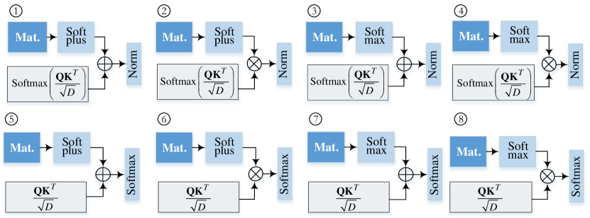
Figure 7: Illustration of enhanced attention variants. By ensuring $\mathbf{B}$ is positive using either Softplus or Softmax, combining it with $\mathbf{A}$ through addition or multiplication, and applying Softmax or Norm for final normalization, we derive seven variants. The first subfigure represents the version adopted by default, while the others are denoted as $\mathrm{Var}\left\{1,\cdots,7\right\}$. Detailed formulas are provided in Table 10.

We present the variants of enhanced attention in Figure 7 and Table 10. For simplicity, our analysis omits the effect of the query matrix $\mathbf{V}$, as it is included in all variants. Notably, the Swin Transformer Liu et al. [2021] introduces relative position bias to the vanilla attention and employs $\mathrm{Softmax}\left(\mathbf{Q}\mathbf{K}^{T}/\sqrt{D}+\mathbf{B}\right)\mathbf{V}$, where $\mathbf{B}$ represents the relative position bias among tokens, with correlations existing between its entries. In contrast, Var4 and Var6 in Table 10, although they exhibit a structure similar to that of the Swin Transformer, allow greater flexibility in $\mathbf{B}$, where each entry is independent. Next, we analyze the Jacobian matrix of the variants without distinguishing between the choices of Softplus and Softmax.

Variants	$\mathrm{EnhAttn}\left(\mathbf{Q},\mathbf{K},\mathbf{V}\right)$
Ours	$\mathrm{Norm}\left(\mathrm{Softmax}\left(\frac{\mathbf{Q}\mathbf{K}^{T}}{\sqrt{D}}\right)+\mathrm{Softplus}(\mathbf{B})\right)\mathbf{V}$
Var1	$\mathrm{Norm}\left(\mathrm{Softmax}\left(\frac{\mathbf{Q}\mathbf{K}^{T}}{\sqrt{D}}\right)\odot\mathrm{Softplus}(\mathbf{B})\right)\mathbf{V}$
Var2	$\mathrm{Norm}\left(\mathrm{Softmax}\left(\frac{\mathbf{Q}\mathbf{K}^{T}}{\sqrt{D}}\right)+\mathrm{Softmax}(\mathbf{B})\right)\mathbf{V}$
Var3	$\mathrm{Norm}\left(\mathrm{Softmax}\left(\frac{\mathbf{Q}\mathbf{K}^{T}}{\sqrt{D}}\right)\odot\mathrm{Softmax}(\mathbf{B})\right)\mathbf{V}$
Var4	$\mathrm{Softmax}\left(\frac{\mathbf{Q}\mathbf{K}^{T}}{\sqrt{D}}+\mathrm{Softplus}(\mathbf{B})\right)\mathbf{V}$
Var5	$\mathrm{Softmax}\left(\frac{\mathbf{Q}\mathbf{K}^{T}}{\sqrt{D}}\odot\mathrm{Softplus}(\mathbf{B})\right)\mathbf{V}$
Var6	$\mathrm{Softmax}\left(\frac{\mathbf{Q}\mathbf{K}^{T}}{\sqrt{D}}+\mathrm{Softmax}(\mathbf{B})\right)\mathbf{V}$
Var7	$\mathrm{Softmax}\left(\frac{\mathbf{Q}\mathbf{K}^{T}}{\sqrt{D}}\odot\mathrm{Softmax}(\mathbf{B})\right)\mathbf{V}$

Table 10: Equations for different variants of the enhanced attention mechanism. These variants correspond to Figure 4 in the main paper.

C.3.1 Var1 and Var3

For Var1 and Var3 in Table 10, the transformation can be simplified to the vector form

$$\mathbf{c}=\mathrm{Norm}\left(\mathrm{Softmax}(\mathbf{a})\odot\mathbf{b}\right)\in\mathbb{R}^{N},$$ (48)

where $\mathbf{b}_{i}>0$ for $i=0,\cdots,N-1$. For simplicity, let $\tilde{\mathbf{a}}\triangleq\mathrm{Softmax}(\mathbf{a})$ and $\tilde{\mathbf{b}}\triangleq\tilde{\mathbf{a}}\odot\mathbf{b}$. The Jacobian matrix of $\mathbf{c}$ with respect to $\mathbf{a}$ can then be expressed as:

$$\frac{\partial\mathbf{c}}{\partial\mathbf{a}}=\frac{\partial\mathbf{c}}{\partial\tilde{\mathbf{b}}}\frac{\partial\tilde{\mathbf{b}}}{\partial\tilde{\mathbf{a}}}\frac{\partial\tilde{\mathbf{a}}}{\partial\mathbf{a}}$$ (49)

$$=\frac{1}{\left\|\tilde{\mathbf{b}}\right\|_{1}^{2}}\left(\left\|\tilde{\mathbf{b}}\right\|_{1}\cdot\mathbf{I}-\tilde{\mathbf{b}}\mathbf{1}^{T}\right)\mathrm{Diag}(\mathbf{b})\left(\mathrm{Diag}(\tilde{\mathbf{a}})-\tilde{\mathbf{a}}\tilde{\mathbf{a}}^{T}\right)$$

$$=\frac{\mathrm{Diag}(\mathbf{b})\left(\mathrm{Diag}(\tilde{\mathbf{a}})-\tilde{\mathbf{a}}\tilde{\mathbf{a}}^{T}\right)}{\left\|\tilde{\mathbf{b}}\right\|_{1}}+\frac{(\mathbf{b}^{T}\tilde{\mathbf{a}})\tilde{\mathbf{b}}\tilde{\mathbf{a}}^{T}-\tilde{\mathbf{b}}\tilde{\mathbf{b}}^{T}}{\left\|\tilde{\mathbf{b}}\right\|_{1}^{2}}.$$

Here, the equations $\mathbf{1}^{T}\mathrm{Diag}(\mathbf{b})=\mathbf{b}^{T}$ and $\mathbf{1}^{T}\mathrm{Diag}(\mathbf{b})\mathrm{Diag}(\tilde{\mathbf{a}})=\mathbf{b}^{T}\mathrm{Diag}(\tilde{\mathbf{a}})=\tilde{\mathbf{b}}^{T}$ are utilized.

Similarly, the Jacobian matrix of $\mathbf{c}$ with respect to $\mathbf{b}$ is:

$$\frac{\partial\mathbf{c}}{\partial\mathbf{b}} =\frac{\partial\mathbf{c}}{\partial\tilde{\mathbf{b}}}\frac{\partial\tilde{\mathbf{b}}}{\partial\mathbf{b}}$$ (50)

$$=\frac{1}{\left\|\tilde{\mathbf{b}}\right\|_{1}^{2}}\left(\left\|\tilde{\mathbf{b}}\right\|_{1}\cdot\mathbf{I}-\tilde{\mathbf{b}}\mathbf{1}^{T}\right)\mathrm{Diag}(\tilde{\mathbf{a}})$$

$$=\frac{1}{\left\|\tilde{\mathbf{b}}\right\|_{1}^{2}}\left(\left\|\tilde{\mathbf{b}}\right\|_{1}\cdot\mathrm{Diag}(\tilde{\mathbf{a}})-\tilde{\mathbf{b}}\tilde{\mathbf{a}}^{T}\right).$$

Despite the complexity of Equation (49), the resulting Jacobian matrix introduces additional weighting and bias factors compared to the vanilla counterpart associated with $\mathrm{Softmax}(\mathbf{a})$, providing greater flexibility to dynamically adjust the gradients.

C.3.2 Var4 and Var6

For Var4 and Var6 in Table 10, the transformation can be simplified to the vector form:

$$\mathbf{c}=\mathrm{Softmax}(\mathbf{a}+\mathbf{b})\in\mathbb{R}^{N},$$ (51)

where $\mathbf{b}_{i}>0$ for $i=0,\cdots,N-1$. According to Equation (40), the Jacobian matrices of $\mathbf{c}$ with respect to $\mathbf{a}$ and $\mathbf{ab}$ can be expressed as:

$$\frac{\partial\mathbf{c}}{\partial\mathbf{a}}=\frac{\partial\mathbf{c}}{\partial\mathbf{b}}=\mathrm{Diag}(\mathbf{c})-\mathbf{c}\mathbf{c}^{T}.$$ (52)

C.3.3 Var5 and Var7

For Var5 and Var7 in Table 10, the transformation can be simplified to the vector form

$$\mathbf{c}=\mathrm{Softmax}(\mathbf{a}\odot\mathbf{b})\in\mathbb{R}^{N},$$ (53)

where $\mathbf{b}_{i}>0$ for $i=0,\cdots,N-1$. For simplicity, let $\tilde{\mathbf{b}}\triangleq\mathbf{a}\odot\mathbf{b}$. The Jacobian matrix of $\mathbf{c}$ with respect to $\mathbf{a}$ is then derived as:

$$\frac{\partial\mathbf{c}}{\partial\mathbf{a}} =\frac{\partial\mathbf{c}}{\partial\tilde{\mathbf{b}}}\frac{\partial\tilde{\mathbf{b}}}{\partial\mathbf{a}}$$ (54)

$$=\left(\mathrm{Diag}(\mathbf{c})-\mathbf{c}\mathbf{c}^{T}\right)\mathrm{Diag}(\mathbf{b}),$$

$$\frac{\partial\mathbf{c}}{\partial\mathbf{b}} =\frac{\partial\mathbf{c}}{\partial\tilde{\mathbf{b}}}\frac{\partial\tilde{\mathbf{b}}}{\partial\mathbf{b}}$$

$$=\left(\mathrm{Diag}(\mathbf{c})-\mathbf{c}\mathbf{c}^{T}\right)\mathrm{Diag}(\mathbf{a}),$$

From Equation (54), we observe that each column of the Jacobian matrix is scaled by the $\mathbf{b}$, introducing additional flexibility in adjusting the gradients.

Performance comparison of these variants are presented in Tables 25, 26, and 27.

Appendix D Dataset Description

In this work, we evaluate the performance of FreEformer on the following real-world datasets:

• ETT Zhou et al. [2021] records seven variables related to electricity transformers from July 2016 to July 2018. It is divided into four datasets: ETTh1 and ETTh2, with hourly readings, and ETTm1 and ETTm2, with readings taken at 15-minute intervals.

• Weather contains 21 meteorological factors (e.g., air temperature, humidity) recorded every 10 minutes at the Weather Station of the Max Planck Biogeochemistry Institute in 2020.

• ECL Wu et al. [2021] documents the hourly electricity consumption of 321 clients from 2012 to 2014.

• Traffic includes hourly road occupancy ratios collected from 862 sensors in the San Francisco Bay Area between January 2015 and December 2016.

• Exchange Wu et al. [2021] features daily exchange rates for eight countries from 1990 to 2016.

• Solar-Energy Lai et al. [2018] captures solar power output from 137 photovoltaic plants in 2006, with data sampled every 10 minutes.

• PEMS Liu et al. [2022a] provides public traffic data from California, collected every 5 minutes. We use the same four subsets (PEMS03, PEMS04, PEMS07, PEMS08) as in SCINet Liu et al. [2022a].

• ILI comprises weekly records of influenza-like illness (ILI) patient counts from the Centers for Disease Control and Prevention in the United States from 2002 to 2021.

• COVID-19 Chen et al. [2022] includes daily COVID-19 hospitalization data in California (CA) from February to December 2020, provided by Johns Hopkins University.

• METR-LA includes traffic network data for Los Angeles, collected from March to June 2012. It contains 207 sensors, with data sampled every 5 minutes.

• NASDAQ comprises daily NASDAQ index data, combined with key economic indicators (e.g., interest rates, exchange rates, gold prices) from 2010 to 2024.

• Wiki contains daily page views for 60,000 Wikipedia articles in eight different languages over two years (2018–2019). We select the first 99 articles as our experimental dataset.

The statistics of these datasets are summarized in Table 11. We split all datasets into training, validation, and test sets in chronological order, using the same splitting ratios as in iTransformer Liu et al. [2024a]. The splitting ratio is set to 6:2:2 for the ETT and PEMS datasets, as well as for the COVID-19 dataset under the ‘input-36-predict-24,36,48,60’ setting. For all other cases (including other datasets and different settings for COVID-19), we use a 7:1:2 split. The reason for this specific setting in the COVID-19 dataset is that its total length is insufficient to accommodate a 7:1:2 split under the ‘input-36-predict-24,36,48,60’ setting.

Datasets	#Variants	Total Len.	Sampling Fre.
ETT{h1, h2}	7	17420	1 hour
ETT{m1, m2}	7	69680	15 min
Weather	21	52696	10 min
ECL	321	26304	1 hour
Traffic	862	17544	1 hour
Exchange	8	7588	1 day
Solar-Energy	137	52560	10 min
PEMS03	358	26209	5 min
PEMS04	307	16992	5 min
PEMS07	883	28224	5 min
PEMS08	170	17856	5 min
ILI	7	966	1 week
COVID-19	55	335	1 day
METR-LA	207	34272	1 day
NASDAQ	12	3914	1 day
Wiki	99	730	1 day

Table 11: Statistics of the real-world datasets utilized in our study

Appendix E Implementation Details

All experiments are implemented in PyTorch Paszke et al. [2019] and conducted on a single NVIDIA 4090 GPU. We optimize the model using the ADAM optimizer Kingma and Ba [2015] with an initial learning rate selected from $\left\{10^{-4},5\times 10^{-4}\right\}$. The model dimension $D$ is chosen from $\left\{128,256,512\right\}$, while the embedding dimension $d$ is fixed at 16. The batch size is determined based on the dataset size and selected from $\left\{4,8,16,32\right\}$. The training is conducted for a maximum of 50 epochs with an early stopping mechanism, which terminates training if the validation performance does not improve for 10 consecutive epochs. We adopt the weighted L1 loss function following CARD Wang et al. [2024c]. For baseline models, we use the reported values from the original papers when available; otherwise, we run the official code. For the recent work FAN Ye et al. [2024], we adopt DLinear as the base forecaster, which is the recommended model in the original paper. Our code is available at this repository: https://anonymous.4open.science/r/FreEformer.

Appendix F Robustness of FreEformer

We report the standard deviation of FreEformer performance under seven runs with different random seeds in Table 12, demonstrating that the performance of FreEformer is stable.

Dataset	ECL		ETTh2		Exchange
Horizon	MSE	MAE	MSE	MAE	MSE	MAE
96	0.133±0.001	0.223±0.001	0.286±0.002	0.335±0.002	0.083±0.001	0.200±0.001
192	0.152±0.001	0.240±0.001	0.363±0.003	0.381±0.002	0.174±0.002	0.296±0.002
336	0.165±0.001	0.256±0.001	0.416±0.003	0.420±0.001	0.325±0.003	0.411±0.002
720	0.198±0.002	0.286±0.002	0.422±0.002	0.436±0.001	0.833±0.009	0.687±0.006
Dataset	Solar-Energy		Traffic		Weather
Horizon	MSE	MAE	MSE	MAE	MSE	MAE
96	0.180±0.001	0.191±0.000	0.395±0.002	0.233±0.000	0.153±0.001	0.189±0.001
192	0.213±0.001	0.215±0.000	0.423±0.004	0.245±0.000	0.201±0.002	0.236±0.002
336	0.233±0.001	0.232±0.000	0.443±0.005	0.254±0.000	0.261±0.003	0.282±0.002
720	0.241±0.001	0.237±0.000	0.480±0.002	0.274±0.000	0.341±0.004	0.334±0.003

Table 12: Robustness of FreEformer performance. The standard deviations are obtained from seven random seeds.

Appendix G Full Results

G.1 Long and Short-Term Forecasting Performance

Model		FreEformer (Ours)		Leddam Yu et al. [2024]		CARD Wang et al. [2024c]		Fredformer Piao et al. [2024]		iTrans. Liu et al. [2024a]		TimeMixer Wang et al. [2024b]		PatchTST Nie et al. [2023]		Crossfm. Zhang and Yan [2023]		TimesNet Wu et al. [2023a]		FreTS Yi et al. [2024c]		DLinear Zeng et al. [2023]
Metric		MSE	MAE	MSE	MAE	MSE	MAE	MSE	MAE	MSE	MAE	MSE	MAE	MSE	MAE	MSE	MAE	MSE	MAE	MSE	MAE	MSE	MAE
	96	0.306	0.340	0.319	0.359	0.316	0.347	0.326	0.361	0.334	0.368	0.320	0.357	0.329	0.367	0.404	0.426	0.338	0.375	0.339	0.374	0.345	0.372
	192	0.359	0.367	0.369	0.383	0.363	0.370	0.363	0.380	0.377	0.391	0.361	0.381	0.367	0.385	0.450	0.451	0.374	0.387	0.382	0.397	0.380	0.389
	336	0.392	0.391	0.394	0.402	0.392	0.390	0.395	0.403	0.426	0.420	0.390	0.404	0.399	0.410	0.532	0.515	0.410	0.411	0.421	0.426	0.413	0.413
	720	0.458	0.428	0.460	0.442	0.458	0.425	0.453	0.438	0.491	0.459	0.454	0.441	0.454	0.439	0.666	0.589	0.478	0.450	0.485	0.462	0.474	0.453
ETTm1	Avg	0.379	0.381	0.386	0.397	0.383	0.384	0.384	0.395	0.407	0.410	0.381	0.395	0.387	0.400	0.513	0.496	0.400	0.406	0.407	0.415	0.403	0.407
	96	0.169	0.248	0.176	0.257	0.169	0.248	0.177	0.259	0.180	0.264	0.175	0.258	0.175	0.259	0.287	0.366	0.187	0.267	0.190	0.282	0.193	0.292
	192	0.233	0.289	0.243	0.303	0.234	0.292	0.243	0.301	0.250	0.309	0.237	0.299	0.241	0.302	0.414	0.492	0.249	0.309	0.260	0.329	0.284	0.362
	336	0.292	0.328	0.303	0.341	0.294	0.339	0.302	0.340	0.311	0.348	0.298	0.340	0.305	0.343	0.597	0.542	0.321	0.351	0.373	0.405	0.369	0.427
	720	0.395	0.389	0.400	0.398	0.390	0.388	0.397	0.396	0.412	0.407	0.391	0.396	0.402	0.400	1.730	1.042	0.408	0.403	0.517	0.499	0.554	0.522
ETTm2	Avg	0.272	0.313	0.281	0.325	0.272	0.317	0.279	0.324	0.288	0.332	0.275	0.323	0.281	0.326	0.757	0.610	0.291	0.333	0.335	0.379	0.350	0.401
	96	0.371	0.390	0.377	0.394	0.383	0.391	0.373	0.392	0.386	0.405	0.375	0.400	0.414	0.419	0.423	0.448	0.384	0.402	0.399	0.412	0.386	0.400
	192	0.424	0.420	0.424	0.422	0.435	0.420	0.433	0.420	0.441	0.436	0.429	0.421	0.460	0.445	0.471	0.474	0.436	0.429	0.453	0.443	0.437	0.432
	336	0.466	0.443	0.459	0.442	0.479	0.442	0.470	0.437	0.487	0.458	0.484	0.458	0.501	0.466	0.570	0.546	0.491	0.469	0.503	0.475	0.481	0.459
	720	0.471	0.470	0.463	0.459	0.471	0.461	0.467	0.456	0.503	0.491	0.498	0.482	0.500	0.488	0.653	0.621	0.521	0.500	0.596	0.565	0.519	0.516
ETTh1	Avg	0.433	0.431	0.431	0.429	0.442	0.429	0.435	0.426	0.454	0.447	0.447	0.440	0.469	0.454	0.529	0.522	0.458	0.450	0.488	0.474	0.456	0.452
	96	0.286	0.335	0.292	0.343	0.281	0.330	0.293	0.342	0.297	0.349	0.289	0.341	0.292	0.342	0.745	0.584	0.340	0.374	0.350	0.403	0.333	0.387
	192	0.363	0.381	0.367	0.389	0.363	0.381	0.371	0.389	0.380	0.400	0.372	0.392	0.387	0.400	0.877	0.656	0.402	0.414	0.472	0.475	0.477	0.476
	336	0.416	0.420	0.412	0.424	0.411	0.418	0.382	0.409	0.428	0.432	0.386	0.414	0.426	0.433	1.043	0.731	0.452	0.452	0.564	0.528	0.594	0.541
	720	0.422	0.436	0.419	0.438	0.416	0.431	0.415	0.434	0.427	0.445	0.412	0.434	0.431	0.446	1.104	0.763	0.462	0.468	0.815	0.654	0.831	0.657
ETTh2	Avg	0.372	0.393	0.373	0.399	0.368	0.390	0.365	0.393	0.383	0.407	0.364	0.395	0.384	0.405	0.942	0.684	0.414	0.427	0.550	0.515	0.559	0.515
	96	0.133	0.223	0.141	0.235	0.141	0.233	0.147	0.241	0.148	0.240	0.153	0.247	0.161	0.250	0.219	0.314	0.168	0.272	0.183	0.269	0.197	0.282
	192	0.152	0.240	0.159	0.252	0.160	0.250	0.165	0.258	0.162	0.253	0.166	0.256	0.199	0.289	0.231	0.322	0.184	0.289	0.187	0.276	0.196	0.285
	336	0.165	0.256	0.173	0.268	0.173	0.263	0.177	0.273	0.178	0.269	0.185	0.277	0.215	0.305	0.246	0.337	0.198	0.300	0.202	0.292	0.209	0.301
	720	0.198	0.286	0.201	0.295	0.197	0.284	0.213	0.304	0.225	0.317	0.225	0.310	0.256	0.337	0.280	0.363	0.220	0.320	0.237	0.325	0.245	0.333
ECL	Avg	0.162	0.251	0.169	0.263	0.168	0.258	0.176	0.269	0.178	0.270	0.182	0.272	0.208	0.295	0.244	0.334	0.192	0.295	0.202	0.290	0.212	0.300
	96	0.083	0.200	0.086	0.207	0.084	0.202	0.084	0.202	0.086	0.206	0.086	0.205	0.088	0.205	0.256	0.367	0.107	0.234	0.086	0.212	0.088	0.218
	192	0.174	0.296	0.175	0.301	0.179	0.298	0.178	0.302	0.177	0.299	0.193	0.312	0.176	0.299	0.470	0.509	0.226	0.344	0.217	0.344	0.176	0.315
	336	0.325	0.411	0.325	0.415	0.333	0.418	0.319	0.408	0.331	0.417	0.356	0.433	0.301	0.397	1.268	0.883	0.367	0.448	0.415	0.475	0.313	0.427
	720	0.833	0.687	0.831	0.686	0.851	0.691	0.749	0.651	0.847	0.691	0.912	0.712	0.901	0.714	1.767	1.068	0.964	0.746	0.947	0.725	0.839	0.695
Exchange	Avg	0.354	0.399	0.354	0.402	0.362	0.402	0.333	0.391	0.360	0.403	0.387	0.416	0.367	0.404	0.940	0.707	0.416	0.443	0.416	0.439	0.354	0.414
	96	0.395	0.233	0.426	0.276	0.419	0.269	0.406	0.277	0.395	0.268	0.462	0.285	0.446	0.283	0.522	0.290	0.593	0.321	0.519	0.315	0.650	0.396
	192	0.423	0.245	0.458	0.289	0.443	0.276	0.426	0.290	0.417	0.276	0.473	0.296	0.540	0.354	0.530	0.293	0.617	0.336	0.521	0.325	0.598	0.370
	336	0.443	0.254	0.486	0.297	0.460	0.283	0.437	0.292	0.433	0.283	0.498	0.296	0.551	0.358	0.558	0.305	0.629	0.336	0.533	0.327	0.605	0.373
	720	0.480	0.274	0.498	0.313	0.490	0.299	0.462	0.305	0.467	0.302	0.506	0.313	0.586	0.375	0.589	0.328	0.640	0.350	0.580	0.344	0.645	0.394
Traffic	Avg	0.435	0.251	0.467	0.294	0.453	0.282	0.433	0.291	0.428	0.282	0.484	0.297	0.531	0.343	0.550	0.304	0.620	0.336	0.538	0.328	0.625	0.383
	96	0.153	0.189	0.156	0.202	0.150	0.188	0.163	0.207	0.174	0.214	0.163	0.209	0.177	0.218	0.158	0.230	0.172	0.220	0.184	0.239	0.196	0.255
	192	0.201	0.236	0.207	0.250	0.202	0.238	0.211	0.251	0.221	0.254	0.208	0.250	0.225	0.259	0.206	0.277	0.219	0.261	0.223	0.275	0.237	0.296
	336	0.261	0.282	0.262	0.291	0.260	0.282	0.267	0.292	0.278	0.296	0.251	0.287	0.278	0.297	0.272	0.335	0.280	0.306	0.272	0.316	0.283	0.335
	720	0.341	0.334	0.343	0.343	0.343	0.353	0.343	0.341	0.358	0.349	0.339	0.341	0.354	0.348	0.398	0.418	0.365	0.359	0.340	0.363	0.345	0.381
Weather	Avg	0.239	0.260	0.242	0.272	0.239	0.265	0.246	0.272	0.258	0.279	0.240	0.271	0.259	0.281	0.259	0.315	0.259	0.287	0.255	0.298	0.265	0.317
	96	0.180	0.191	0.197	0.241	0.197	0.211	0.185	0.233	0.203	0.237	0.189	0.259	0.234	0.286	0.310	0.331	0.250	0.292	0.192	0.225	0.290	0.378
	192	0.213	0.215	0.231	0.264	0.234	0.234	0.227	0.253	0.233	0.261	0.222	0.283	0.267	0.310	0.734	0.725	0.296	0.318	0.229	0.252	0.320	0.398
	336	0.233	0.232	0.241	0.268	0.256	0.250	0.246	0.284	0.248	0.273	0.231	0.292	0.290	0.315	0.750	0.735	0.319	0.330	0.242	0.269	0.353	0.415
	720	0.241	0.237	0.250	0.281	0.260	0.254	0.247	0.276	0.249	0.275	0.223	0.285	0.289	0.317	0.769	0.765	0.338	0.337	0.240	0.272	0.356	0.413
Solar-Energy	Avg	0.217	0.219	0.230	0.264	0.237	0.237	0.226	0.262	0.233	0.262	0.216	0.280	0.270	0.307	0.641	0.639	0.301	0.319	0.226	0.254	0.330	0.401
1st Count		21	30	4	0	8	13	5	7	4	0	8	0	1	1	0	0	0	0	0	0	0	0

Table 13: Full results of long-term multivariate time series forecasting results for prediction lengths $\tau\in\left\{96,192,336,720\right\}$ with the lookback length being 96. Results for the PEMS datasets are provided in Table 14.

Model		FreEformer (Ours)		Leddam Yu et al. [2024]		CARD Wang et al. [2024c]		Fredformer Piao et al. [2024]		iTrans. Liu et al. [2024a]		TimeMixer Wang et al. [2024b]		PatchTST Nie et al. [2023]		Crossfm. Zhang and Yan [2023]		TimesNet Wu et al. [2023a]		FreTS Yi et al. [2024c]		DLinear Zeng et al. [2023]
Metric		MSE	MAE	MSE	MAE	MSE	MAE	MSE	MAE	MSE	MAE	MSE	MAE	MSE	MAE	MSE	MAE	MSE	MAE	MSE	MAE	MSE	MAE
	12	0.060	0.160	0.063	0.164	0.072	0.177	0.068	0.174	0.071	0.174	0.076	0.188	0.099	0.216	0.090	0.203	0.085	0.192	0.083	0.194	0.122	0.243
	24	0.077	0.181	0.080	0.185	0.107	0.217	0.094	0.205	0.093	0.201	0.113	0.226	0.142	0.259	0.121	0.240	0.118	0.223	0.127	0.241	0.201	0.317
	48	0.112	0.218	0.124	0.226	0.194	0.302	0.152	0.262	0.125	0.236	0.191	0.292	0.211	0.319	0.202	0.317	0.155	0.260	0.202	0.310	0.333	0.425
	96	0.159	0.265	0.160	0.266	0.323	0.402	0.228	0.330	0.164	0.275	0.288	0.363	0.269	0.370	0.262	0.367	0.228	0.317	0.265	0.365	0.457	0.515
PEMS03	Avg	0.102	0.206	0.107	0.210	0.174	0.275	0.135	0.243	0.113	0.221	0.167	0.267	0.180	0.291	0.169	0.281	0.147	0.248	0.169	0.278	0.278	0.375
	12	0.068	0.164	0.071	0.172	0.089	0.194	0.085	0.189	0.078	0.183	0.092	0.204	0.105	0.224	0.098	0.218	0.087	0.195	0.097	0.209	0.148	0.272
	24	0.079	0.179	0.087	0.193	0.128	0.234	0.117	0.224	0.095	0.205	0.128	0.243	0.153	0.275	0.131	0.256	0.103	0.215	0.144	0.258	0.224	0.340
	48	0.099	0.204	0.113	0.222	0.224	0.321	0.174	0.276	0.120	0.233	0.213	0.315	0.229	0.339	0.205	0.326	0.136	0.250	0.223	0.328	0.355	0.437
	96	0.129	0.238	0.141	0.252	0.382	0.445	0.273	0.354	0.150	0.262	0.307	0.384	0.291	0.389	0.402	0.457	0.190	0.303	0.288	0.379	0.452	0.504
PEMS04	Avg	0.094	0.196	0.103	0.210	0.206	0.299	0.162	0.261	0.111	0.221	0.185	0.287	0.195	0.307	0.209	0.314	0.129	0.241	0.188	0.294	0.295	0.388
	12	0.053	0.138	0.055	0.145	0.068	0.166	0.063	0.158	0.067	0.165	0.073	0.184	0.095	0.207	0.094	0.200	0.082	0.181	0.078	0.185	0.115	0.242
	24	0.067	0.153	0.070	0.164	0.103	0.206	0.089	0.192	0.088	0.190	0.111	0.219	0.150	0.262	0.139	0.247	0.101	0.204	0.127	0.239	0.210	0.329
	48	0.087	0.174	0.094	0.192	0.165	0.268	0.136	0.241	0.110	0.215	0.237	0.328	0.253	0.340	0.311	0.369	0.134	0.238	0.220	0.317	0.398	0.458
	96	0.115	0.205	0.117	0.217	0.258	0.346	0.197	0.298	0.139	0.245	0.303	0.354	0.346	0.404	0.396	0.442	0.181	0.279	0.316	0.386	0.594	0.553
PEMS07	Avg	0.080	0.167	0.084	0.180	0.149	0.247	0.121	0.222	0.101	0.204	0.181	0.271	0.211	0.303	0.235	0.315	0.124	0.225	0.185	0.282	0.329	0.395
	12	0.066	0.157	0.071	0.171	0.080	0.181	0.081	0.185	0.079	0.182	0.091	0.201	0.168	0.232	0.165	0.214	0.112	0.212	0.096	0.204	0.154	0.276
	24	0.085	0.176	0.091	0.189	0.118	0.220	0.112	0.214	0.115	0.219	0.137	0.246	0.224	0.281	0.215	0.260	0.141	0.238	0.152	0.256	0.248	0.353
	48	0.119	0.207	0.128	0.219	0.199	0.289	0.174	0.267	0.186	0.235	0.265	0.343	0.321	0.354	0.315	0.355	0.198	0.283	0.247	0.331	0.440	0.470
	96	0.169	0.238	0.198	0.266	0.405	0.431	0.277	0.335	0.221	0.267	0.410	0.407	0.408	0.417	0.377	0.397	0.320	0.351	0.354	0.395	0.674	0.565
PEMS08	Avg	0.110	0.194	0.122	0.211	0.201	0.280	0.161	0.250	0.150	0.226	0.226	0.299	0.280	0.321	0.268	0.307	0.193	0.271	0.212	0.297	0.379	0.416
1st Count		20	20	0	0	0	0	0	0	0	0	0	0	0	0	0	0	0	0	0	0	0	0

Table 14: Full results of long-term multivariate time series forecasting for the PEMS datasets. The prediction lengths are $\tau\in\left\{96,192,336,720\right\}$ and the lookback length is 96. The bast and second-best results are highlighted in bold and underlined, respectively.

Model		FreEformer (Ours)		Leddam Yu et al. [2024]		CARD Wang et al. [2024c]		Fredformer Piao et al. [2024]		iTrans. Liu et al. [2024a]		TimeMixer Wang et al. [2024b]		PatchTST Nie et al. [2023]		TimesNet Wu et al. [2023a]		DLinear Zeng et al. [2023]		FreTS Yi et al. [2024c]
Metric		MSE	MAE	MSE	MAE	MSE	MAE	MSE	MAE	MSE	MAE	MSE	MAE	MSE	MAE	MSE	MAE	MSE	MAE	MSE	MAE
	3	0.508	0.366	0.551	0.388	0.597	0.392	0.528	0.403	0.555	0.395	0.659	0.435	0.646	0.417	0.627	0.420	1.280	0.747	0.647	0.416
	6	0.898	0.522	1.021	0.569	1.246	0.610	1.128	0.604	1.124	0.586	1.306	0.643	1.269	0.629	1.147	0.610	2.054	0.967	1.503	0.720
	9	1.277	0.648	1.881	0.795	2.041	0.829	1.804	0.786	1.794	0.772	2.070	0.842	2.021	0.830	1.796	0.785	2.771	1.138	2.250	0.935
	12	1.876	0.805	2.421	0.964	2.746	0.996	2.610	0.989	2.273	0.884	2.792	1.018	2.788	1.016	2.349	0.920	3.497	1.284	2.956	1.058
	Avg	1.140	0.585	1.468	0.679	1.658	0.707	1.518	0.696	1.437	0.659	1.707	0.734	1.681	0.723	1.480	0.684	2.400	1.034	1.839	0.782
	24	1.980	0.849	2.085	0.883	2.407	0.970	2.098	0.894	2.004	0.860	2.110	0.879	2.046	0.849	2.317	0.934	3.158	1.243	2.804	1.107
	36	1.879	0.823	2.017	0.892	2.324	0.948	1.712	0.867	1.910	0.880	2.084	0.890	2.344	0.912	1.972	0.920	3.009	1.200	2.881	1.136
	48	1.825	0.815	1.860	0.847	2.133	0.911	2.054	0.922	2.036	0.891	1.961	0.866	2.123	0.883	2.238	0.940	2.994	1.194	3.074	1.195
	60	1.940	0.852	1.967	0.879	2.177	0.921	1.925	0.913	2.022	0.919	1.926	0.878	2.001	0.895	2.027	0.928	3.172	1.232	3.384	1.258
ILI	Avg	1.906	0.835	1.982	0.875	2.260	0.938	1.947	0.899	1.993	0.887	2.020	0.878	2.128	0.885	2.139	0.931	3.083	1.217	3.036	1.174
	3	1.094	0.498	1.216	0.570	1.103	0.521	1.165	0.548	1.193	0.561	1.237	0.547	1.220	0.573	2.021	0.704	2.386	0.909	1.196	0.552
	6	1.726	0.624	1.782	0.689	1.919	0.735	1.465	0.685	1.933	0.755	2.003	0.739	1.982	0.762	2.405	0.808	3.220	1.053	2.221	0.794
	9	2.238	0.741	2.407	0.866	2.358	0.841	2.145	0.845	2.441	0.879	2.594	0.860	2.633	0.916	2.858	0.969	3.803	1.160	3.193	1.018
	12	2.509	0.828	2.851	0.991	2.857	0.971	2.833	0.984	2.819	0.984	3.103	0.981	3.050	1.030	2.993	0.964	4.524	1.288	3.455	1.086
	Avg	1.892	0.673	2.064	0.779	2.059	0.767	1.902	0.765	2.096	0.795	2.234	0.782	2.221	0.820	2.569	0.861	3.483	1.102	2.516	0.862
	24	4.452	1.230	4.860	1.342	5.133	1.394	4.799	1.347	4.715	1.321	6.335	1.554	5.528	1.450	5.634	1.442	9.780	1.851	6.587	1.528
	36	6.844	1.621	7.378	1.708	7.377	1.725	7.536	1.727	7.299	1.681	8.222	1.787	8.351	1.830	9.114	1.848	12.804	2.083	10.431	1.913
	48	10.209	2.009	10.051	1.999	11.013	2.103	9.833	1.951	10.141	2.012	11.669	2.157	11.259	2.114	10.940	2.033	14.244	2.189	13.354	2.135
	60	12.235	2.196	11.467	2.119	12.528	2.227	12.455	2.209	11.871	2.156	12.188	2.173	12.666	2.225	12.888	2.186	15.472	2.275	15.008	2.255
COVID-19	Avg	8.435	1.764	8.439	1.792	9.013	1.862	8.656	1.808	8.506	1.792	9.604	1.918	9.451	1.905	9.644	1.877	13.075	2.099	11.345	1.958
	3	0.208	0.172	0.204	0.191	0.210	0.180	0.205	0.188	0.205	0.188	0.205	0.192	0.204	0.190	0.221	0.204	0.218	0.231	0.202	0.211
	6	0.301	0.208	0.293	0.227	0.311	0.219	0.298	0.227	0.300	0.229	0.297	0.230	0.298	0.227	0.308	0.238	0.307	0.278	0.292	0.261
	9	0.383	0.239	0.369	0.264	0.401	0.253	0.385	0.263	0.386	0.265	0.381	0.264	0.382	0.263	0.387	0.273	0.386	0.316	0.371	0.305
	12	0.453	0.264	0.442	0.292	0.474	0.281	0.457	0.292	0.460	0.295	0.455	0.295	0.456	0.292	0.462	0.298	0.452	0.353	0.431	0.340
	Avg	0.336	0.221	0.327	0.243	0.349	0.233	0.336	0.242	0.338	0.244	0.334	0.245	0.335	0.243	0.344	0.253	0.341	0.294	0.324	0.279
	24	0.648	0.339	0.680	0.405	0.700	0.378	0.676	0.408	0.700	0.413	0.671	0.413	0.679	0.410	0.698	0.415	0.645	0.458	0.637	0.448
	36	0.792	0.389	0.841	0.471	0.874	0.448	0.852	0.477	0.867	0.480	0.841	0.480	0.845	0.484	0.856	0.475	0.785	0.533	0.769	0.520
	48	0.910	0.431	0.963	0.528	1.017	0.498	0.982	0.526	1.017	0.539	0.964	0.531	0.972	0.536	0.972	0.518	0.885	0.585	0.872	0.582
	60	1.010	0.464	1.029	0.556	1.126	0.541	1.084	0.569	1.079	0.572	1.047	0.573	1.077	0.578	1.033	0.543	0.959	0.623	0.938	0.624
METR-LA	Avg	0.840	0.406	0.878	0.490	0.929	0.466	0.898	0.495	0.916	0.501	0.881	0.499	0.893	0.502	0.890	0.488	0.819	0.550	0.804	0.543
	3	0.035	0.092	0.040	0.103	0.037	0.096	0.039	0.102	0.040	0.105	0.035	0.093	0.038	0.099	0.049	0.123	0.044	0.123	0.045	0.129
	6	0.049	0.118	0.054	0.128	0.052	0.123	0.053	0.126	0.054	0.129	0.049	0.118	0.053	0.124	0.061	0.142	0.062	0.155	0.076	0.180
	9	0.062	0.137	0.066	0.147	0.063	0.141	0.067	0.147	0.068	0.150	0.062	0.139	0.065	0.145	0.073	0.161	0.082	0.189	0.103	0.216
	12	0.075	0.156	0.078	0.164	0.075	0.158	0.079	0.165	0.078	0.165	0.073	0.156	0.077	0.161	0.088	0.179	0.100	0.215	0.098	0.213
	Avg	0.055	0.126	0.059	0.135	0.057	0.130	0.059	0.135	0.060	0.137	0.055	0.126	0.058	0.132	0.068	0.151	0.072	0.170	0.080	0.184
	24	0.119	0.216	0.125	0.222	0.124	0.220	0.128	0.226	0.137	0.237	0.122	0.221	0.127	0.224	0.198	0.299	0.155	0.274	0.173	0.294
	36	0.166	0.263	0.174	0.271	0.167	0.266	0.170	0.268	0.184	0.280	0.183	0.279	0.174	0.269	0.229	0.326	0.196	0.306	0.200	0.309
	48	0.204	0.298	0.222	0.312	0.218	0.307	0.218	0.306	0.229	0.318	0.200	0.298	0.225	0.314	0.267	0.352	0.244	0.344	0.302	0.393
	60	0.250	0.331	0.264	0.341	0.264	0.341	0.262	0.339	0.279	0.352	0.238	0.328	0.265	0.339	0.327	0.394	0.318	0.401	0.380	0.449
NASDAQ	Avg	0.185	0.277	0.196	0.286	0.193	0.284	0.194	0.285	0.207	0.297	0.186	0.281	0.198	0.286	0.255	0.343	0.228	0.331	0.263	0.361
	3	6.153	0.371	6.148	0.383	6.183	0.378	6.190	0.387	6.237	0.393	6.209	0.392	6.112	0.380	7.597	0.510	6.254	0.438	6.227	0.424
	6	6.443	0.386	6.455	0.397	6.465	0.393	6.696	0.404	6.484	0.400	6.475	0.402	6.425	0.395	7.962	0.515	6.579	0.467	6.426	0.441
	9	6.659	0.399	6.687	0.412	6.714	0.415	6.768	0.411	6.689	0.411	6.702	0.418	6.743	0.426	8.150	0.524	6.776	0.508	6.660	0.458
	12	6.842	0.409	6.899	0.424	6.852	0.415	7.168	0.424	6.868	0.419	6.902	0.426	6.814	0.414	8.117	0.533	6.927	0.513	6.772	0.468
	Avg	6.524	0.391	6.547	0.404	6.553	0.400	6.705	0.406	6.569	0.405	6.572	0.409	6.523	0.404	7.956	0.520	6.634	0.481	6.521	0.448
	24	6.887	0.424	6.919	0.450	6.925	0.440	6.531	0.432	6.886	0.437	6.900	0.446	6.858	0.430	8.023	0.612	6.883	0.520	6.809	0.484
	36	6.436	0.440	6.456	0.457	6.463	0.451	5.935	0.453	6.431	0.452	6.520	0.467	6.400	0.445	7.229	0.595	6.393	0.538	6.340	0.497
	48	6.012	0.449	6.031	0.468	6.031	0.460	5.871	0.464	6.101	0.483	6.108	0.484	5.959	0.449	7.184	0.641	5.940	0.547	5.897	0.519
	60	5.699	0.456	5.740	0.478	5.723	0.463	5.389	0.463	5.681	0.462	5.732	0.476	5.633	0.452	6.805	0.645	5.605	0.552	5.543	0.520
Wiki	Avg	6.259	0.442	6.286	0.463	6.285	0.453	5.931	0.453	6.275	0.458	6.315	0.468	6.212	0.444	7.310	0.623	6.205	0.539	6.147	0.505
1st Count		22	46	2	1	0	0	10	1	0	0	7	5	2	3	0	0	0	0	11	0

Table 15: Full results of short-term multivariate time series forecasting. Two settings are used for comparison: ‘Input-12-Predict-{3,6,9,12}’ and ‘Input-36-Predict-{24,36,48,60}’. The best and second-best results are highlighted in bold and underlined, respectively.

Tables 13 and 14 present the comprehensive results for long-term multivariate time series forecasting, serving as the full version of Table 1 in the main paper. Specifically, FreEformer consistently outperforms state-of-the-art models across all prediction lengths for the PEMS datasets, demonstrating its robust performance advantage.

Table 15 provides the comprehensive results for short-term multivariate time series forecasting under two lookback-prediction settings: ‘Input-12-Predict-{3,6,9,12}’ and ‘Input-36-Predict-{24,36,48,60}’. Despite the limited sizes of the ILI, COVID-19, NASDAQ and Wiki datasets, FreEformer consistently outperforms state-of-the-art models. Interestingly, the linear and frequency-based model FreTS shows competitive performance, likely due to the strong inductive bias of frequency modeling.

G.2 Enhanced Attention Generality

Model		iTrans.				PatchTST				Leddam				Fredformer
		Van. Attn.		Enh. Attn.		Van. Attn.		Enh. Attn.		Van. Attn.		Enh. Attn.		Van. Attn.		Enh. Attn.
Metric		MSE	MAE	MSE	MAE	MSE	MAE	MSE	MAE	MSE	MAE	MSE	MAE	MSE	MAE	MSE	MAE
ETTm1	96	0.334	0.368	0.322	0.360	0.329	0.367	0.322	0.360	0.319	0.359	0.319	0.359	0.326	0.361	0.324	0.360
	192	0.377	0.391	0.365	0.383	0.367	0.385	0.362	0.384	0.369	0.383	0.367	0.382	0.363	0.380	0.364	0.381
	336	0.426	0.420	0.399	0.405	0.399	0.410	0.390	0.407	0.394	0.402	0.392	0.400	0.395	0.403	0.394	0.404
	720	0.491	0.459	0.469	0.444	0.454	0.439	0.449	0.437	0.460	0.442	0.459	0.440	0.453	0.438	0.456	0.440
	Avg	0.407	0.410	0.389	0.398	0.211	0.303	0.381	0.397	0.386	0.397	0.384	0.395	0.384	0.396	0.385	0.396
Weather	96	0.174	0.214	0.161	0.207	0.177	0.218	0.162	0.206	0.156	0.202	0.156	0.202	0.163	0.207	0.155	0.202
	192	0.221	0.254	0.213	0.253	0.225	0.259	0.208	0.250	0.207	0.250	0.205	0.248	0.211	0.251	0.206	0.248
	336	0.278	0.296	0.271	0.297	0.278	0.297	0.265	0.291	0.262	0.291	0.262	0.291	0.267	0.292	0.266	0.291
	720	0.358	0.349	0.353	0.350	0.354	0.348	0.347	0.345	0.343	0.343	0.343	0.343	0.343	0.341	0.340	0.341
	Avg	0.258	0.278	0.249	0.276	0.211	0.303	0.245	0.273	0.242	0.272	0.242	0.271	0.246	0.273	0.242	0.271
ECL	96	0.148	0.240	0.137	0.232	0.161	0.250	0.154	0.245	0.141	0.235	0.139	0.234	0.147	0.241	0.139	0.236
	192	0.162	0.253	0.154	0.248	0.199	0.289	0.166	0.256	0.159	0.252	0.158	0.252	0.165	0.258	0.158	0.254
	336	0.178	0.269	0.169	0.264	0.215	0.305	0.183	0.273	0.173	0.268	0.172	0.269	0.177	0.273	0.175	0.272
	720	0.225	0.317	0.200	0.296	0.256	0.337	0.221	0.307	0.201	0.295	0.198	0.294	0.213	0.304	0.203	0.297
	Avg	0.178	0.270	0.165	0.260	0.208	0.295	0.181	0.270	0.169	0.263	0.167	0.262	0.176	0.269	0.169	0.265
Solar-Energy	96	0.203	0.237	0.194	0.233	0.234	0.286	0.201	0.244	0.197	0.241	0.192	0.224	0.185	0.233	0.148	0.246
	192	0.233	0.261	0.225	0.258	0.267	0.310	0.232	0.264	0.231	0.264	0.231	0.255	0.227	0.253	0.237	0.273
	336	0.248	0.273	0.241	0.273	0.290	0.315	0.249	0.275	0.241	0.268	0.245	0.264	0.246	0.284	0.254	0.283
	720	0.249	0.275	0.245	0.277	0.289	0.317	0.248	0.276	0.250	0.281	0.245	0.276	0.247	0.276	0.250	0.287
	Avg	0.233	0.262	0.226	0.260	0.211	0.303	0.232	0.265	0.230	0.264	0.228	0.255	0.226	0.262	0.222	0.272
PEMS03	12	0.071	0.174	0.062	0.164	0.099	0.216	0.071	0.175	0.063	0.164	0.062	0.165	0.068	0.174	0.063	0.164
	24	0.093	0.201	0.079	0.185	0.142	0.259	0.103	0.211	0.080	0.185	0.078	0.182	0.094	0.205	0.082	0.188
	48	0.125	0.236	0.113	0.222	0.211	0.319	0.168	0.266	0.124	0.226	0.112	0.219	0.152	0.262	0.125	0.234
	96	0.164	0.275	0.154	0.266	0.269	0.370	0.251	0.328	0.160	0.266	0.160	0.264	0.228	0.330	0.165	0.276
	Avg	0.113	0.222	0.102	0.209	0.211	0.303	0.148	0.245	0.107	0.210	0.103	0.208	0.135	0.243	0.109	0.215
PEMS07	12	0.067	0.165	0.055	0.145	0.095	0.207	0.065	0.161	0.055	0.145	0.054	0.144	0.063	0.158	0.059	0.152
	24	0.088	0.190	0.069	0.161	0.150	0.262	0.097	0.193	0.070	0.164	0.068	0.161	0.089	0.192	0.079	0.175
	48	0.110	0.215	0.096	0.190	0.253	0.340	0.214	0.312	0.094	0.192	0.087	0.183	0.136	0.241	0.113	0.211
	96	0.139	0.245	0.124	0.219	0.346	0.404	0.250	0.311	0.117	0.217	0.113	0.214	0.197	0.298	0.163	0.259
	Avg	0.101	0.204	0.086	0.179	0.211	0.303	0.156	0.244	0.084	0.180	0.080	0.175	0.121	0.222	0.103	0.199
METR-LA	3	0.205	0.188	0.204	0.190	0.204	0.190	0.204	0.190	0.204	0.191	0.208	0.193	0.205	0.188	0.204	0.188
	6	0.300	0.229	0.294	0.227	0.298	0.227	0.298	0.229	0.293	0.227	0.294	0.229	0.298	0.227	0.294	0.227
	9	0.386	0.265	0.374	0.261	0.382	0.263	0.382	0.263	0.369	0.264	0.360	0.259	0.385	0.263	0.385	0.261
	12	0.460	0.295	0.444	0.292	0.456	0.292	0.456	0.293	0.442	0.292	0.420	0.290	0.457	0.292	0.453	0.290
	Avg	0.338	0.244	0.329	0.243	0.211	0.303	0.335	0.244	0.327	0.243	0.321	0.243	0.336	0.242	0.334	0.242

Table 16: Applying enhanced attention to Transformer-based forecasters. Consistent performance improvements are observed when replacing vanilla attention with the enhanced version, leaving other components unchanged. The lookback length is 12 for METR-LA and 96 for all other datasets.

To evaluate the generality of the enhanced attention mechanism, we integrate it into several state-of-the-art Transformer-based forecasters, including iTransformer, PatchTST, Leddam, and Fredformer. Only the attention mechanism is updated, while other components and the loss function remain unchanged. Notably, Leddam and Fredformer are more sophisticated than iTransformer and PatchTST, and the updated modules in Leddam and Fredformer constitute only a small portion of their overall architectures. For instance, only the ‘channel-wise self-attention’ module is updated in Leddam.

Table 16 shows that replacing vanilla attention with the enhanced version consistently improves performance. On the PEMS07 dataset, the enhanced attention achieves average MSE improvements of 14.9% for iTransformer, 25.9% for PatchTST, 4.1% for Leddam, and 14.6% for Fredformer. This demonstrates the effectiveness and general applicability of the enhanced attention. Table 16 provides the full results corresponding to Table 9 in the main paper.

Figures 8, 9, 10, and 11 show the attention matrices of iTransformer, PatchTST, Leddam, and Fredformer, respectively. After incorporating the learnable matrix, the final attention matrix demonstrates higher rank and more prominent values.

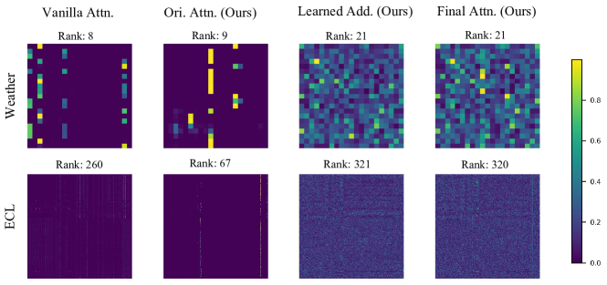
Figure 8: Attention matrices of iTransformer from vanilla and enhanced attention. The left column shows the low-rank attention matrix from the vanilla self-attention mechanism (Weather: 8, ECL: 260), with most entries near zero. The right three columns show the original attention matrix ($\mathbf{A}$), the learned addition matrix ($\mathrm{Softplus}(\mathbf{B})$), and the final attention matrix ($\mathrm{Norm}\left(\mathbf{A}+\mathrm{Softplus}(\mathbf{B})\right)$). The final attention matrix, after incorporating the learned matrix, exhibits more prominent values and higher ranks (Weather: 21, ECL: 320).

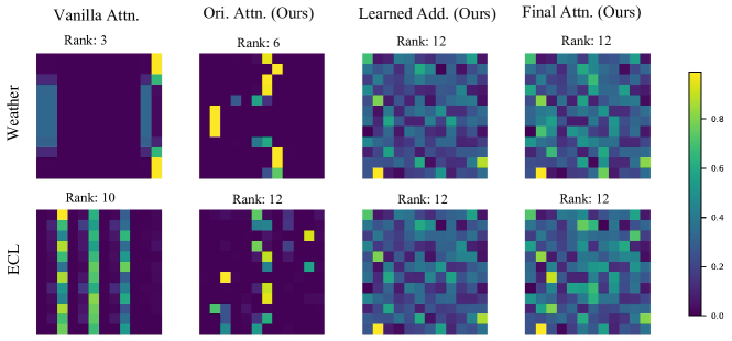
Figure 9: Attention matrices of PatchTST from vanilla and enhanced attention. The left column shows the low-rank attention matrix from the vanilla self-attention mechanism (Weather: 3, ECL: 10), with most entries near zero. The right three columns show the original attention matrix ($\mathbf{A}$), the learned addition matrix ($\mathrm{Softplus}(\mathbf{B})$), and the final attention matrix ($\mathrm{Norm}\left(\mathbf{A}+\mathrm{Softplus}(\mathbf{B})\right)$). The final attention matrix, after incorporating the learned matrix, exhibits more prominent values and higher ranks (Weather: 12, ECL: 12).

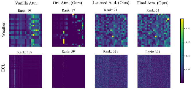
Figure 10: Attention matrices of Leddam from vanilla and enhanced attention. The left column shows the low-rank attention matrix from the vanilla self-attention mechanism (Weather: 19, ECL: 178), with most entries near zero. The right three columns show the original attention matrix ($\mathbf{A}$), the learned addition matrix ($\mathrm{Softplus}(\mathbf{B})$), and the final attention matrix ($\mathrm{Norm}\left(\mathbf{A}+\mathrm{Softplus}(\mathbf{B})\right)$). The final attention matrix, after incorporating the learned matrix, exhibits more prominent values and higher ranks (Weather: 21, ECL: 321).

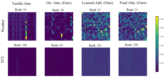
Figure 11: Attention matrices of Fredformer from vanilla and enhanced attention. The left column shows the low-rank attention matrix from the vanilla self-attention mechanism (Weather: 16, ECL: 196), with most entries near zero. The right three columns show the original attention matrix ($\mathbf{A}$), the learned addition matrix ($\mathrm{Softplus}(\mathbf{B})$), and the final attention matrix ($\mathrm{Norm}\left(\mathbf{A}+\mathrm{Softplus}(\mathbf{B})\right)$). The final attention matrix, after incorporating the learned matrix, exhibits more prominent values and higher ranks (Weather: 21, ECL: 320).

G.3 Full Results of Architecture Ablations

				ETTm1		Weather		ECL		Traffic		COVID-19
Layer	Dim.	Patch.	$\tau$	MSE	MAE	MSE	MAE	MSE	MAE	MSE	MAE	MSE	MAE
			96 / 3	0.312	0.343	0.155	0.194	0.165	0.258	0.463	0.298	1.152	0.510
			192 / 6	0.364	0.370	0.209	0.242	0.173	0.265	0.473	0.304	1.815	0.661
			336 / 9	0.397	0.391	0.268	0.287	0.190	0.283	0.488	0.310	2.374	0.798
			720 / 12	0.466	0.429	0.347	0.338	0.230	0.315	0.527	0.331	2.819	0.927
Linear	Variate	✗	Avg	0.385	0.383	0.245	0.265	0.189	0.280	0.488	0.311	2.040	0.724
			96 / 3	0.316	0.347	0.163	0.199	0.157	0.241	0.457	0.272	1.112	0.510
			192 / 6	0.366	0.372	0.208	0.241	0.168	0.251	0.467	0.276	1.830	0.686
			336 / 9	0.398	0.393	0.266	0.284	0.186	0.269	0.484	0.283	2.443	0.841
			720 / 12	0.463	0.430	0.345	0.336	0.225	0.302	0.519	0.301	2.960	0.979
Linear	Fre.	✗	Avg	0.386	0.385	0.246	0.265	0.184	0.266	0.482	0.283	2.086	0.754
			96 / 3	0.308	0.340	0.162	0.197	0.153	0.236	0.474	0.254	1.116	0.516
			192 / 6	0.363	0.370	0.209	0.242	0.167	0.251	0.485	0.261	1.843	0.688
			336 / 9	0.394	0.391	0.263	0.282	0.186	0.268	0.507	0.268	2.425	0.828
			720 / 12	0.459	0.428	0.343	0.336	0.225	0.300	0.550	0.286	3.019	0.997
Trans.	Fre.	✔	Avg	0.381	0.382	0.244	0.264	0.183	0.264	0.504	0.267	2.100	0.757
			96 / 3	0.309	0.342	0.162	0.199	0.154	0.239	0.465	0.271	1.118	0.506
			192 / 6	0.366	0.371	0.209	0.243	0.166	0.250	0.473	0.277	1.872	0.702
			336 / 9	0.396	0.393	0.266	0.286	0.183	0.267	0.493	0.283	2.445	0.835
			720 / 12	0.461	0.430	0.342	0.336	0.223	0.301	0.527	0.301	3.028	0.985
Trans.	Fre.	✗	Avg	0.383	0.384	0.245	0.266	0.181	0.264	0.489	0.283	2.116	0.757
			96 / 3	0.315	0.349	0.157	0.195	0.134	0.225	0.408	0.241	1.101	0.513
			192 / 6	0.361	0.372	0.204	0.241	0.152	0.242	0.422	0.252	1.812	0.692
			336 / 9	0.400	0.399	0.265	0.287	0.166	0.257	0.450	0.262	2.356	0.821
			720 / 12	0.463	0.435	0.339	0.335	0.196	0.284	0.491	0.277	2.848	0.960
Trans.	Variate	✔	Avg	0.385	0.389	0.241	0.264	0.162	0.252	0.443	0.258	2.029	0.747
			96 / 3	0.306	0.340	0.153	0.189	0.133	0.223	0.395	0.233	1.094	0.498
			192 / 6	0.359	0.367	0.201	0.236	0.152	0.240	0.423	0.245	1.726	0.624
			336 / 9	0.392	0.391	0.261	0.282	0.165	0.256	0.443	0.254	2.238	0.741
			720 / 12	0.458	0.428	0.341	0.334	0.198	0.286	0.480	0.274	2.509	0.828
Trans.	Variate	✗	Avg	0.379	0.381	0.239	0.260	0.162	0.251	0.435	0.251	1.892	0.673

Table 17: Complete results of architecture ablation studies on layers, dimensions, and patching settings. The layers include linear and Transformer layers, and the dimensions refer to frequency and variate dimensions. ‘Patch.’ indicates patching along the frequency dimension. The patch length and stride are 6 and 3 for COVID-19, and 16 and 8 for other datasets. Prediction lengths are $\tau\in{3,6,9,12}$ for COVID-19 and $\tau\in{96,192,336,720}$ for other datasets. The final setting corresponds to the FreEformer configuration. This table is the extended version of Table 5 in the main paper.

Table 17 is the full version of Table 5 in the main paper, showing complete results for the architecture ablations of FreEformer. FreEformer consistently outperforms its variants with alternative layer, dimension, and patching settings.

G.4 Comparison With Other Attention Mechanisms

Model		Ours		Informer Zhou et al. [2021]		Flowformer Wu et al. [2022]		Flashformer Dao et al. [2022]		FLatten Han et al. [2023]		Mamba Gu and Dao [2023]		LASER Surya Duvvuri and Dhillon [2024]		Lin.Attn. Yue et al. [2024]
Metric		MSE	MAE	MSE	MAE	MSE	MAE	MSE	MAE	MSE	MAE	MSE	MAE	MSE	MAE	MSE	MAE
	96	0.395	0.233	0.412	0.235	0.413	0.234	0.445	0.273	0.409	0.235	0.408	0.252	0.410	0.235	0.415	0.235
	192	0.423	0.245	0.441	0.247	0.437	0.246	0.422	0.245	0.440	0.247	0.432	0.264	0.439	0.247	0.438	0.246
	336	0.443	0.254	0.455	0.255	0.460	0.256	0.446	0.252	0.462	0.254	0.450	0.272	0.458	0.254	0.458	0.254
	720	0.480	0.274	0.489	0.274	0.504	0.275	0.481	0.272	0.504	0.272	0.484	0.291	0.498	0.271	0.496	0.272
Traffic	Avg	0.435	0.251	0.449	0.253	0.453	0.253	0.448	0.260	0.453	0.252	0.443	0.270	0.451	0.252	0.452	0.252
	12	0.060	0.160	0.062	0.163	0.063	0.164	0.064	0.165	0.064	0.165	0.065	0.166	0.064	0.166	0.065	0.166
	24	0.077	0.181	0.079	0.184	0.083	0.189	0.084	0.190	0.085	0.190	0.086	0.192	0.084	0.190	0.084	0.189
	48	0.112	0.218	0.113	0.221	0.132	0.238	0.130	0.236	0.127	0.234	0.127	0.234	0.122	0.230	0.130	0.235
	96	0.159	0.265	0.158	0.263	0.176	0.280	0.179	0.283	0.181	0.284	0.182	0.285	0.174	0.279	0.182	0.284
PEMS03	Avg	0.102	0.206	0.103	0.208	0.113	0.218	0.114	0.218	0.114	0.218	0.115	0.219	0.111	0.216	0.115	0.218
	96	0.153	0.189	0.152	0.191	0.156	0.191	0.163	0.198	0.167	0.200	0.160	0.197	0.162	0.197	0.162	0.197
	192	0.201	0.236	0.204	0.238	0.209	0.242	0.208	0.241	0.212	0.246	0.206	0.241	0.210	0.245	0.208	0.242
	336	0.261	0.282	0.268	0.285	0.263	0.284	0.264	0.283	0.267	0.286	0.262	0.283	0.263	0.282	0.266	0.285
	720	0.341	0.334	0.345	0.338	0.342	0.336	0.345	0.338	0.346	0.339	0.343	0.336	0.343	0.337	0.344	0.337
Weather	Avg	0.239	0.260	0.242	0.263	0.242	0.263	0.245	0.265	0.248	0.267	0.243	0.264	0.244	0.265	0.245	0.265
	96	0.180	0.191	0.183	0.194	0.186	0.195	0.182	0.193	0.200	0.200	0.189	0.201	0.180	0.194	0.205	0.202
	192	0.213	0.215	0.214	0.216	0.221	0.219	0.221	0.220	0.227	0.221	0.223	0.224	0.220	0.219	0.228	0.222
	336	0.233	0.232	0.237	0.234	0.243	0.235	0.236	0.235	0.240	0.235	0.243	0.239	0.236	0.236	0.240	0.236
	720	0.241	0.237	0.243	0.239	0.248	0.241	0.244	0.240	0.248	0.243	0.256	0.245	0.242	0.241	0.247	0.242
Solar-Energy	Avg	0.217	0.219	0.219	0.221	0.224	0.222	0.221	0.222	0.229	0.224	0.228	0.227	0.219	0.222	0.230	0.225
	3	0.508	0.366	0.542	0.357	0.580	0.394	0.596	0.417	0.614	0.385	0.615	0.389	0.590	0.402	0.447	0.354
	6	0.898	0.522	1.239	0.540	0.959	0.515	1.129	0.553	1.181	0.565	1.109	0.567	1.054	0.540	1.074	0.542
	9	1.277	0.648	1.360	0.640	1.519	0.720	1.777	0.722	1.450	0.710	1.858	0.779	1.502	0.732	1.778	0.754
	12	1.876	0.805	2.850	0.807	2.096	0.816	2.686	0.870	4.125	0.949	2.450	0.887	3.238	0.860	2.513	0.845
ILI	Avg	1.140	0.585	1.498	0.586	1.288	0.611	1.547	0.640	1.842	0.652	1.508	0.655	1.596	0.633	1.453	0.624

Table 18: Comparison with state-of-the-art attention models using the FreEformer architecture. The best and second-best results are highlighted in bold and underlined, respectively. The lookback length is set to 96, except for the ILI dataset, where it is set to 12.

We further compare the enhanced attention with state-of-the-art attention models using the FreEformer architecture. As shown in Table 18, the enhanced attention consistently outperforms other attention paradigms, despite requiring only minimal modifications to the vanilla attention mechanism and being easy to implement. Table 18 is the complete version of Table 8 in the main paper.

Appendix H More Experiments

H.1 Best Performance with Varying Lookback Lengths

Model		FreEformer		Leddam		CARD		Fredformer		iTrans.		TimeMixer		PatchTST		TimesNet		DLinear
Metric		MSE	MAE	MSE	MAE	MSE	MAE	MSE	MAE	MSE	MAE	MSE	MAE	MSE	MAE	MSE	MAE	MSE	MAE
	96	0.124	0.214	0.134	0.227	0.129	0.223	0.129	0.226	0.132	0.227	0.129	0.224	0.129	0.222	0.168	0.272	0.140	0.237
	192	0.142	0.232	0.156	0.248	0.154	0.245	0.148	0.244	0.154	0.251	0.140	0.220	0.147	0.240	0.184	0.322	0.153	0.249
	336	0.158	0.248	0.166	0.264	0.161	0.257	0.165	0.262	0.170	0.268	0.161	0.255	0.163	0.259	0.198	0.300	0.169	0.267
	720	0.185	0.274	0.195	0.291	0.185	0.278	0.193	0.286	0.193	0.288	0.194	0.287	0.197	0.290	0.220	0.320	0.203	0.301
ECL	Avg	0.152	0.242	0.163	0.257	0.157	0.251	0.159	0.254	0.162	0.258	0.156	0.247	0.159	0.253	0.193	0.304	0.166	0.264
	96	0.341	0.225	0.366	0.260	0.341	0.229	0.358	0.257	0.359	0.262	0.360	0.249	0.360	0.249	0.593	0.321	0.410	0.282
	192	0.369	0.234	0.394	0.270	0.367	0.243	0.381	0.272	0.376	0.270	0.375	0.250	0.379	0.256	0.617	0.336	0.423	0.287
	336	0.387	0.241	0.400	0.283	0.388	0.254	0.396	0.277	0.393	0.279	0.385	0.270	0.392	0.264	0.629	0.336	0.436	0.296
	720	0.424	0.260	0.442	0.297	0.427	0.276	0.424	0.296	0.434	0.293	0.430	0.281	0.432	0.286	0.640	0.350	0.466	0.315
Traffic	Avg	0.380	0.240	0.400	0.278	0.381	0.251	0.390	0.275	0.390	0.276	0.388	0.263	0.391	0.264	0.620	0.336	0.434	0.295
	96	0.144	0.185	0.149	0.199	0.145	0.186	0.150	0.203	0.165	0.214	0.147	0.197	0.149	0.198	0.172	0.220	0.176	0.237
	192	0.190	0.230	0.196	0.243	0.187	0.227	0.194	0.246	0.208	0.253	0.189	0.239	0.194	0.241	0.219	0.261	0.220	0.282
	336	0.238	0.268	0.243	0.280	0.238	0.258	0.243	0.284	0.257	0.292	0.241	0.280	0.306	0.282	0.246	0.337	0.265	0.319
	720	0.319	0.325	0.321	0.334	0.308	0.321	0.308	0.333	0.331	0.343	0.310	0.330	0.314	0.334	0.365	0.359	0.323	0.362
Weather	Avg	0.223	0.252	0.227	0.264	0.220	0.248	0.224	0.266	0.240	0.275	0.222	0.262	0.241	0.264	0.251	0.294	0.246	0.300
	96	0.160	0.196	0.186	0.242	0.170	0.207	0.187	0.236	0.190	0.241	0.167	0.220	0.224	0.278	0.219	0.314	0.289	0.377
	192	0.190	0.212	0.208	0.262	0.192	0.219	0.196	0.251	0.233	0.261	0.187	0.249	0.253	0.298	0.231	0.322	0.319	0.397
	336	0.195	0.219	0.218	0.265	0.226	0.233	0.208	0.265	0.226	0.275	0.200	0.258	0.273	0.306	0.246	0.337	0.352	0.415
	720	0.206	0.224	0.208	0.273	0.217	0.243	0.209	0.272	0.220	0.282	0.215	0.250	0.272	0.308	0.280	0.363	0.356	0.412
Solar-Energy	Avg	0.188	0.213	0.205	0.261	0.201	0.225	0.200	0.256	0.217	0.265	0.192	0.244	0.256	0.298	0.244	0.334	0.329	0.400
	96	0.282	0.332	0.294	0.347	0.288	0.332	0.284	0.338	0.309	0.357	0.291	0.340	0.293	0.346	0.338	0.375	0.299	0.343
	192	0.323	0.358	0.336	0.369	0.332	0.357	0.323	0.364	0.346	0.383	0.327	0.365	0.333	0.370	0.374	0.387	0.335	0.365
	336	0.358	0.378	0.364	0.389	0.364	0.376	0.358	0.387	0.385	0.410	0.360	0.381	0.369	0.392	0.410	0.411	0.369	0.386
	720	0.405	0.413	0.421	0.419	0.414	0.407	0.420	0.417	0.440	0.442	0.415	0.417	0.416	0.420	0.478	0.450	0.425	0.421
ETTm1	Avg	0.342	0.370	0.354	0.381	0.350	0.368	0.346	0.376	0.370	0.398	0.348	0.376	0.353	0.382	0.400	0.406	0.357	0.379

Table 19: Best performance using varying lookback lengths. The best and second-best results are highlighted in bold and underlined, respectively. For FreEformer, the lookback length is chosen from {96,192,336,720}.

We further evaluate forecasting performance under varying lookback lengths. Unlike the constant lookback length setting in the main paper, we explore optimal performance with lookback lengths selected from {96, 192, 336, 720}. As shown in Table 19, FreEformer achieves state-of-the-art performance across various forecasting horizons and datasets under this setting, demonstrating its robust forecasting capabilities.

H.2 More Metrics

To provide a more comprehensive evaluation of forecasting models, we introduce the following scale-free metrics: Coefficient of Determination ($R^{2}$), Pearson Correlation Coefficient ($r$), and Mean Absolute Scaled Error (MASE). These metrics are calculated as follows:

$$R^{2}=\frac{1}{N}\sum_{n=1}^{N}\left(1-\frac{\left|\hat{\mathbf{y}}_{n:}-\mathbf{y}_{n:}\right|^{2}_{2}}{\left|\mathbf{y}_{n:}-\overline{\mathbf{y}_{n:}}\right|^{2}_{2}}\right),$$ (55)

$$r=\frac{1}{N}\sum_{n=1}^{N}\frac{{\textstyle\sum_{t=1}^{\tau}}\left(\hat{\mathbf{y}}_{n,t}-\overline{\hat{\mathbf{y}}_{n:}}\right)\left(\mathbf{y}_{n,t}-\overline{\mathbf{y}_{n:}}\right)}{\sqrt{{\textstyle\sum_{t=1}^{\tau}}\left(\hat{\mathbf{y}}_{n,t}-\overline{\hat{\mathbf{y}}_{n:}}\right)^{2}}\sqrt{{\textstyle\sum_{t=1}^{\tau}}\left(\mathbf{y}_{n,t}-\overline{\mathbf{y}_{n:}}\right)^{2}}},$$

$$\mathrm{MASE}=\frac{1}{N}\sum_{n=1}^{N}\frac{\frac{1}{\tau}\left\|\hat{\mathbf{y}}_{n:}-\mathbf{y}_{n:}\right\|_{1}}{\frac{1}{\tau-1}{\textstyle\sum_{t=1}^{\tau-1}\left|\mathbf{y}_{n,t}-\mathbf{y}_{t-1,n}\right|}}.$$

Here, $\mathbf{y}\in\mathbb{R}^{N\times\tau}$ and $\hat{\mathbf{y}}\in\mathbb{R}^{N\times\tau}$ denote the ground truth and predictions, respectively, and $\overline{(\cdot)}$ represents the mean value.

As shown in Table 20, FreEformer outperforms state-of-the-art models on the ECL and Traffic datasets under these metrics, demonstrating its robustness.

Model		FreEformer			Leddam			CARD			iTrans.
Metric		$R^{2}$ ($\uparrow$)	r ($\uparrow$)	MASE ($\downarrow$)	$R^{2}$ ($\uparrow$)	r ($\uparrow$)	MASE ($\downarrow$)	$R^{2}$ ($\uparrow$)	r ($\uparrow$)	MASE ($\downarrow$)	$R^{2}$ ($\uparrow$)	r ($\uparrow$)	MASE ($\downarrow$)
	96	0.617	0.915	0.913	0.527	0.911	0.964	0.533	0.905	0.975	0.550	0.907	0.990
	192	0.623	0.907	0.990	0.593	0.902	1.041	0.547	0.899	1.028	0.590	0.900	1.057
	336	0.705	0.899	1.074	0.670	0.893	1.134	0.678	0.891	1.113	0.678	0.893	1.133
	720	0.686	0.885	1.202	0.661	0.882	1.251	0.653	0.877	1.273	0.638	0.872	1.315
ECL	Avg	0.658	0.901	1.045	0.613	0.897	1.098	0.603	0.893	1.097	0.614	0.893	1.124
	96	0.731	0.895	0.748	0.681	0.885	0.909	0.690	0.882	0.855	0.690	0.889	0.860
	192	0.713	0.881	0.772	0.666	0.865	0.949	0.683	0.869	0.856	0.689	0.877	0.879
	336	0.724	0.872	0.771	0.707	0.867	0.897	0.702	0.862	0.843	0.713	0.867	0.883
	720	0.698	0.857	0.824	0.687	0.853	0.947	0.679	0.848	0.894	0.693	0.857	0.913
Traffic	Avg	0.716	0.876	0.779	0.685	0.868	0.926	0.689	0.865	0.862	0.696	0.873	0.884
Model		TimeMixer			DLinear			PatchTST			TimesNet
Metric		$R^{2}$ ($\uparrow$)	r ($\uparrow$)	MASE ($\downarrow$)	$R^{2}$ ($\uparrow$)	r ($\uparrow$)	MASE ($\downarrow$)	$R^{2}$ ($\uparrow$)	r ($\uparrow$)	MASE ($\downarrow$)	$R^{2}$ ($\uparrow$)	r ($\uparrow$)	MASE ($\downarrow$)
	96	0.456	0.897	1.022	0.120	0.870	1.300	0.426	0.890	1.119	0.405	0.892	1.118
	192	0.575	0.893	1.076	0.215	0.867	1.312	0.509	0.887	1.140	0.503	0.885	1.195
	336	0.640	0.886	1.155	0.247	0.858	1.387	0.604	0.880	1.216	0.592	0.875	1.262
	720	0.634	0.871	1.314	0.148	0.844	1.536	0.605	0.864	1.371	0.603	0.864	1.388
ECL	Avg	0.576	0.887	1.142	0.182	0.860	1.384	0.536	0.880	1.211	0.526	0.879	1.241
	96	0.640	0.888	0.979	0.441	0.811	1.346	0.668	0.880	0.903	0.625	0.877	1.023
	192	0.660	0.862	0.959	0.551	0.815	1.189	0.677	0.871	0.887	0.635	0.867	1.009
	336	0.685	0.852	0.960	0.582	0.810	1.167	0.700	0.863	0.874	0.654	0.852	1.079
	720	0.672	0.842	0.986	0.564	0.794	1.224	0.681	0.850	0.925	0.661	0.850	1.047
Traffic	Avg	0.664	0.861	0.971	0.535	0.808	1.232	0.682	0.866	0.897	0.644	0.862	1.040

Table 20: Forecasting performance on the $R^{2}$, Correlation Coefficient ($r$), and MASE metrics. The best and second-best results are highlighted in bold and underlined, respectively. The symbols $\downarrow$ and $\uparrow$ indicate that lower and higher values are preferable, respectively. The lookback length is uniformly set to 96.

H.3 Lookback Length

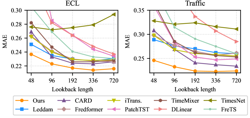
Figure 12: Performance comparison under various lookback lengths, with a fixed prediction horizon of 96.

Increasing the lookback length $T$ improves frequency resolution, which is inversely proportional to $T$ (specifically, $1/T$) Palani [2022], leading to more refined frequency representations. Figure 12 illustrates the MAE changes under different lookback lengths. FreEformer exhibits improved performance with increasing lookback length, consistently outperforming the state-of-the-art forecasters across all lookback lengths on the ECL and Traffic datasets.

H.4 Limited Training Data

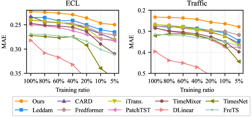
Figure 13: Performance comparison under various training ratios using the Input-96-Predict-96 setting. The y-axis is inverted for improved readability.

Evaluating model performance with limited training data highlights a model’s learning efficiency and robustness. As illustrated in Figure 13, FreEformer consistently outperforms state-of-the-art forecasters, including frequency-based models (FreTS and Fredformer), across all training ratios, from 100% to as low as 5%. This demonstrates the effectiveness of our frequency modeling approach, which explores multivariate correlations in the frequency spectrum, and the strength of the overall model design.

H.5 Comparison with Large Pre-Trained Models

Train. Ratio	100%		20%		5%		0% (Zero-shot)
Model	Ours	Timer Liu et al. [2024b]	Ours	Timer Liu et al. [2024b]	Ours	Timer Liu et al. [2024b]	Timer-28B Liu et al. [2024b]	Moirai-L Woo et al. [2024]	Moment Goswami et al. [2024]	TimesFM Das et al. [2023]	Chronos-S20 Ansari et al. [2024]
Pre-trained	No	UTSD-12G	No	UTSD-12G	No	UTSD-12G	UTSD+LOTSA	LOTSA	TS Pile	N/A	Public Data
Look-back	Best	672	Best	672	Best	672	672	512	512	512	512
ETTh1	0.370	0.358	0.402	0.359	0.427	0.362	0.393	0.394	0.674	0.414	0.454
ETTh2	0.284	–	0.294	0.284	0.315	0.280	0.308	0.293	0.330	0.318	0.326
ETTm1	0.282	–	0.307	0.321	0.320	0.321	0.420	0.452	0.670	0.354	0.451
ETTm2	0.165	–	0.168	0.187	0.178	0.176	0.247	0.214	0.257	0.201	0.190
ECL	0.124	0.136	0.133	0.134	0.145	0.132	0.147	0.155	0.744	-	-
Traffic	0.341	0.351	0.375	0.352	0.425	0.361	0.414	0.399	1.293	-	-
Weather	0.144	0.154	0.161	0.151	0.175	0.151	0.243	0.221	0.255	-	-
PEMS03	0.060	0.118	0.121	0.116	0.232	0.125	-	-	-	-	-
PEMS04	0.068	0.107	0.201	0.120	0.815	0.135	-	-	-	-	-

Table 21: Comparison with pre-trained time series models. The better results are highlighted in bold. The MSE is reported and the prediction length is set to 96.

We further compare FreEformer’s performance with existing pre-trained time series models under fine-tuning scenarios. Surprisingly, as shown in Table 21, FreEformer outperforms the pre-trained model Timer Liu et al. [2024b] on the Traffic, Weather, PEMS03, and PEMS04 datasets, even when Timer is fine-tuned using the full training set. Remarkably, with only 20% of the training data, FreEformer achieves better performance than Timer on the ETTm1, ETTm2, and ECL datasets. These results provide several key insights: 1) The proposed model demonstrates robust forecasting performance even with limited training data; 2) Current pre-trained time series models still require extensive fine-tuning to achieve optimal downstream performance; 3) The scale and diversity of existing time series corpora for pre-training remain limited, and the development of pre-trained time series models is still in its early stages.

H.6 Efficiency

As shown in Figure 14, FreEformer achieves a favorable trade-off between performance and training efficiency, thanks to its relatively simple frequency-modeling architecture. Detailed comparisons of resource consumption during the training and inference stages between FreEformer and state-of-the-art forecasters are provided in Table 22.

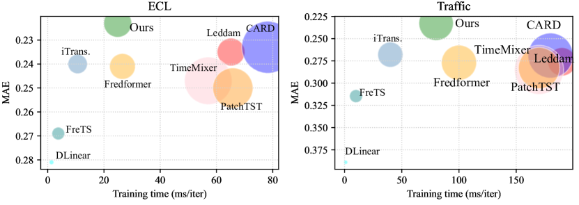
Figure 14: Comparison of model efficiency. Lookback and prediction lengths are both 96, with a fixed batch size of 16. The Y-axis is inverted for clarity. Bubble area is proportional to training GPU memory usage. For improved visual presentation, bubbles within each subfigure are scaled by a uniform factor.

Models		FreEformer	Leddam	CARD	Fredformer	iTrans.	TimeMixer	DLinear	TimesNet	PatchTST	FreTS
ETTh1	Params(M)	10.63	8.55	0.03	8.59	4.83	0.08	0.02	299.94	3.76	0.42
	FLOPS(M)	61.51	111.54	1.41	135.01	33.99	10.72	0.13	289708	272.20	2.94
	T.T. (ms/iter)	23.33	23.54	29.10	26.48	10.11	27.99	1.42	501.98	8.37	3.63
	T.M.(GB)	0.26	0.18	0.03	0.24	0.21	0.05	0.02	5.80	0.14	0.03
	I.T.(ms/iter)	2.92	2.62	4.05	3.73	1.72	3.86	0.21	155.97	1.38	0.49
	I.M. (MB)	179.80	51.04	11.02	78.04	156.00	18.06	8.48	1396.24	51.83	14.47
ECL	Params(M)	11.05	8.56	1.39	12.117	4.83	0.12	0.02	300.58	3.76	0.42
	FLOPS(G)	3.23	5.32	5.07	5.55	1.87	1.74	0.01	293.98	12.48	0.13
	T.T. (ms/iter)	24.89	65.19	78.25	26.587	10.66	57.09	1.37	509.17	65.83	3.78
	T.M.(GB)	1.46	1.44	5.08	1.24	0.70	4.24	0.04	5.82	3.02	0.30
	I.T.(ms/iter)	6.42	14.78	28.21	7.08	3.46	22.79	0.20	157.13	20.52	0.48
	I.M. (GB)	0.38	0.49	0.63	0.26	0.23	0.82	0.02	1.41	0.93	0.23
Exchange	Params(M)	10.63	8.56	1.39	8.59	4.83	0.08	0.02	299.94	3.76	0.42
	FLOPS(M)	70.33	127.49	114.83	135.01	38.88	12.25	0.15	287909	311.08	3.36
	T.T. (ms/iter)	23.25	24.81	35.57	28.56	10.14	27.46	1.47	505.39	9.75	3.51
	T.M.(GB)	0.26	0.18	0.17	0.24	0.21	0.06	0.02	5.80	0.15	0.03
	I.T.(ms/iter)	2.91	2.62	6.02	6.86	1.70	3.81	0.21	156.33	2.47	0.48
	I.M. (GB)	0.18	0.05	0.03	0.08	0.16	0.02	0.01	1.40	0.05	0.02
Traffic	Params(M)	13.61	8.56	0.98	11.09	4.83	0.12	0.02	301.69	3.76	0.42
	FLOPS(G)	10.59	15.24	10.47	14.78	6.45	4.66	0.02	288.72	33.52	0.36
	T.T. (s/iter)	0.08	0.19	0.18	0.10	0.04	0.17	0.001	0.50	0.17	0.01
	T.M.(GB)	5.52	3.74	9.50	5.76	2.95	11.33	0.07	5.86	8.01	0.78
	I.T.(ms/iter)	25.11	45.68	61.21	31.60	13.45	67.21	0.20	15.64	55.10	3.48
	I.M. (GB)	1.51	1.25	1.69	1.84	1.27	2.20	0.04	1.42	2.44	0.59
Weather	Params(M)	10.64	8.56	0.03	0.50	4.83	0.10	0.02	299.97	3.76	0.42
	FLOPS(G)	0.19	0.34	0.004	0.01	0.10	0.05	0.000	291.21	0.82	0.01
	T.T. (ms/iter)	23.25	27.55	28.69	37.85	9.45	33.30	1.38	505.88	9.89	3.53
	T.M.(GB)	0.30	0.21	0.05	0.05	0.22	0.16	0.02	5.80	0.27	0.04
	I.T.(ms/iter)	2.90	3.15	4.11	7.19	1.66	5.10	0.20	156.27	2.96	0.48
	I.M. (MB)	63.96	70.06	14.45	18.28	34.88	36.03	9.06	1397.18	90.78	24.37
Solar-Energy	Params(M)	10.71	8.56	1.39	4.61	4.83	0.12	0.02	300.21	3.76	0.42
	FLOPS(G)	1.28	2.22	2.05	1.20	0.72	0.74	0.003	290.64	5.33	0.06
	T.T. (ms/iter)	23.35	48.64	36.28	31.77	9.97	35.90	1.44	506.58	28.89	3.60
	T.M.(GB)	0.62	0.68	2.22	0.61	0.37	1.83	0.03	5.81	1.34	0.15
	I.T.(ms/iter)	2.94	7.65	10.44	5.16	1.96	8.54	0.20	156.66	8.49	0.48
	I.M. (GB)	0.24	0.23	0.28	0.16	0.18	0.36	0.01	1.40	0.42	0.11
PEMS07	Params(M)	13.76	8.56	1.39	13.44	4.83	0.12	0.02	301.73	3.76	0.42
	FLOPS(G)	10.93	15.65	16.10	20.53	6.66	4.77	0.02	290.97	34.34	0.37
	T.T. (s/iter)	0.11	0.19	0.28	0.11	0.04	0.17	0.002	0.51	0.18	0.01
	T.M.(GB)	7.65	3.85	13.99	6.42	3.07	11.62	0.07	5.86	8.20	0.79
	I.T.(ms/iter)	20.80	47.06	94.01	36.54	13.92	68.96	0.20	156.78	8.19	0.50
	I.M. (GB)	1.95	1.28	1.74	2.03	1.32	2.25	0.04	1.43	2.50	0.61

Table 22: Resource utilization of the FreEformer and state-of-the-art forecasters on various real-world datasets under the ‘input-96-predict-96’ setting. The table reports the number of parameters, FLOPS, training time (T.T.), training memory usage (T.M.), inference time (I.T.), and inference memory usage (I.M.). FLOPS calculations are performed using the fvcore library and the batch size is fixed as 16.

Appendix I More Ablation Studies

I.1 On More Bases Beyond Fourier

Fourier and wavelet bases are among the most commonly used orthogonal bases in signal processing. For the wavelet bases, we choose two types: the classic Haar and discrete Meyer wavelets. The approximation and detail coefficients are processed independently, similar to how the real and imaginary parts are handled in FreEformer. In addition to Fourier and wavelet bases, we also evaluate three polynomial bases: Legendre, Chebyshev, and Laguerre, which are defined as follows:

$$\mathrm{Legendre}_{k}(t) =\frac{1}{2^{k}k!}\frac{d^{k}}{dt^{k}}\left[\left(t^{2}-1\right)^{k}\right],$$ (56)

$$\mathrm{Chebyshev}_{k}(t) =\mathrm{cos}\left(k\cdot\mathrm{arccos}\left(t\right)\right),$$

$$\mathrm{Laguerre}_{k}(t) =e^{t}\frac{d^{k}}{dt^{k}}\left(e^{-t}t^{k}\right).$$

Here, $\mathrm{Legendre}_{k}(t)$, $\mathrm{Chebyshev}_{k}(t)$, and $\mathrm{Laguerre}_{k}(t)$ represent the $k$-th polynomial basis for Legendre, Chebyshev, and Laguerre bases, respectively. These bases are real-valued polynomials that are orthogonal over specific intervals, with the Chebyshev and Laguerre bases being orthogonal under certain weight functions.

We replace Fourier bases with the aforementioned bases and present the results in Table 23. For comparison, we also include results without any transformation (denoted as ‘Identity’), which correspond to the temporal representation in Table 6 of the main paper. As shown in Table 23, Fourier bases generally outperform the other bases, achieving average MSE improvements of 8.4%, 6.9%, and 2.2% compared to the Identity, polynomial, and wavelet bases, respectively. The wavelet bases also perform well, even slightly outperforming Fourier bases on the PEMS03 dataset. Exploring more robust basis functions is a promising direction for future research.

		Weather		Traffic		Solar		PEMS03		ILI
Base	Horizon	MSE	MAE	MSE	MAE	MSE	MAE	MSE	MAE	MSE	MAE
	H1	0.153	0.189	0.395	0.233	0.180	0.191	0.060	0.160	0.508	0.366
	H2	0.201	0.236	0.423	0.245	0.213	0.215	0.077	0.181	0.898	0.522
	H3	0.261	0.282	0.443	0.254	0.233	0.232	0.112	0.218	1.277	0.648
	H4	0.341	0.334	0.480	0.274	0.241	0.237	0.159	0.265	1.876	0.805
Fourier (Ours)	Avg	0.239	0.260	0.435	0.251	0.217	0.219	0.102	0.206	1.140	0.585
	H1	0.158	0.193	0.391	0.233	0.193	0.205	0.061	0.161	0.601	0.390
	H2	0.204	0.239	0.424	0.246	0.228	0.227	0.080	0.184	0.960	0.533
	H3	0.266	0.283	0.450	0.255	0.254	0.244	0.118	0.221	1.390	0.670
	H4	0.345	0.335	0.489	0.274	0.263	0.250	0.171	0.271	1.752	0.790
Legendre	Avg	0.243	0.263	0.438	0.252	0.234	0.231	0.108	0.209	1.176	0.596
	H1	0.157	0.193	0.405	0.249	0.190	0.204	0.064	0.164	0.537	0.370
	H2	0.202	0.237	0.429	0.260	0.227	0.226	0.084	0.187	0.859	0.523
	H3	0.268	0.287	0.453	0.267	0.251	0.242	0.122	0.223	1.746	0.738
	H4	0.344	0.336	0.484	0.287	0.261	0.246	0.177	0.275	2.723	0.890
Chebyshev	Avg	0.243	0.263	0.443	0.265	0.232	0.229	0.112	0.212	1.466	0.630
	H1	0.161	0.197	0.409	0.243	0.193	0.204	0.066	0.168	0.631	0.415
	H2	0.208	0.243	0.421	0.255	0.228	0.225	0.086	0.191	1.182	0.637
	H3	0.270	0.287	0.451	0.263	0.253	0.244	0.123	0.228	1.688	0.771
	H4	0.350	0.340	0.488	0.283	0.262	0.249	0.177	0.273	2.153	0.893
Laguerre	Avg	0.247	0.267	0.442	0.261	0.234	0.230	0.113	0.215	1.413	0.679
	H1	0.156	0.190	0.408	0.231	0.182	0.192	0.062	0.165	0.568	0.394
	H2	0.203	0.239	0.440	0.245	0.213	0.213	0.077	0.180	0.986	0.532
	H3	0.260	0.280	0.461	0.253	0.234	0.231	0.108	0.215	1.461	0.686
	H4	0.350	0.340	0.498	0.272	0.243	0.237	0.152	0.257	1.987	0.805
Wavelet1	Avg	0.242	0.262	0.452	0.250	0.218	0.218	0.100	0.204	1.250	0.604
	H1	0.156	0.191	0.409	0.232	0.183	0.196	0.061	0.159	0.486	0.358
	H2	0.206	0.239	0.439	0.245	0.216	0.219	0.077	0.180	0.942	0.521
	H3	0.272	0.286	0.463	0.254	0.238	0.235	0.105	0.213	1.390	0.668
	H4	0.345	0.336	0.503	0.274	0.248	0.240	0.150	0.257	2.024	0.827
Wavelet2	Avg	0.244	0.263	0.453	0.251	0.221	0.222	0.098	0.202	1.210	0.593
	H1	0.155	0.191	0.399	0.234	0.187	0.198	0.062	0.162	0.494	0.352
	H2	0.205	0.239	0.431	0.246	0.221	0.219	0.079	0.183	0.889	0.503
	H3	0.268	0.287	0.454	0.255	0.246	0.238	0.116	0.220	1.328	0.657
	H4	0.343	0.335	0.488	0.273	0.259	0.245	0.232	0.320	2.791	0.861
Identity	Avg	0.243	0.263	0.443	0.252	0.228	0.225	0.122	0.221	1.375	0.593

Table 23: Ablation studies on additional polynomial and wavelet bases. For ‘Wavelet1’ and ‘Wavelet2’, we employ the classic Haar and discrete Meyer wavelets, respectively. ‘Identity’ indicates no transformation, corresponding to the temporal representation shown in Table 6 of the main paper. The lookback length $T$ and prediction horizons $\left(\mathrm{H}1,\mathrm{H}2,\mathrm{H}3,\mathrm{H}4\right)$ are configured as follows. Weather, Traffic, and Solar-Energy datasets: $T=96$; $\left(\mathrm{H}1,\mathrm{H}2,\mathrm{H}3,\mathrm{H}4\right)=\left(96,192,336,720\right)$. PEMS03 dataset: $T=96$; $\left(\mathrm{H}1,\mathrm{H}2,\mathrm{H}3,\mathrm{H}4\right)=\left(12,24,48,96\right)$. ILI dataset: $T=12$; $\left(\mathrm{H}1,\mathrm{H}2,\mathrm{H}3,\mathrm{H}4\right)=\left(3,6,9,12\right)$. For Legendre, Chebyshev, and Laguerre bases, we select the number of basis functions from the set $\{5,\mathrm{T}\}$ and report the better results.

I.2 Module Ablations

To verify the effectiveness of the frequency-domain representation and enhanced attention modules, we conduct ablation studies on these two components. As shown in Table 24, both modules consistently improve performance. On these datasets, the frequency-domain representation yields an average improvement of 6.2%, while the enhanced attention mechanism provides an additional improvement of 4.9%.

				Weather		ECL		Traffic		Solar-Energy		PEMS03		ILI
Base	Fre.	Enh.Attn.	Horizon	MSE	MAE	MSE	MAE	MSE	MAE	MSE	MAE	MSE	MAE	MSE	MAE
			H1	0.171	0.202	0.139	0.228	0.394	0.238	0.189	0.199	0.065	0.168	0.667	0.380
			H2	0.208	0.240	0.157	0.245	0.429	0.251	0.221	0.220	0.090	0.197	1.155	0.551
			H3	0.263	0.282	0.174	0.261	0.455	0.256	0.241	0.237	0.139	0.245	2.190	0.769
			H4	0.349	0.338	0.197	0.283	0.488	0.273	0.252	0.243	0.291	0.363	4.547	0.975
✔			Avg	0.248	0.266	0.167	0.254	0.441	0.254	0.226	0.225	0.146	0.243	2.140	0.669
			H1	0.163	0.198	0.137	0.226	0.411	0.235	0.182	0.195	0.065	0.167	0.493	0.368
			H2	0.207	0.240	0.155	0.242	0.436	0.246	0.221	0.220	0.084	0.190	1.124	0.548
			H3	0.265	0.283	0.170	0.258	0.457	0.253	0.234	0.233	0.124	0.231	1.880	0.737
			H4	0.344	0.337	0.197	0.284	0.502	0.273	0.243	0.241	0.181	0.284	2.545	0.847
✔	✔		Avg	0.245	0.264	0.165	0.252	0.451	0.252	0.220	0.222	0.113	0.218	1.510	0.625
			H1	0.153	0.189	0.133	0.223	0.395	0.233	0.180	0.191	0.060	0.160	0.508	0.366
			H2	0.201	0.236	0.152	0.240	0.423	0.245	0.213	0.215	0.077	0.181	0.898	0.522
			H3	0.261	0.282	0.165	0.256	0.443	0.254	0.233	0.232	0.112	0.218	1.277	0.648
			H4	0.341	0.334	0.198	0.286	0.480	0.274	0.241	0.237	0.159	0.265	1.876	0.805
✔	✔	✔	Avg	0.239	0.260	0.162	0.251	0.435	0.251	0.217	0.219	0.102	0.206	1.140	0.585

Table 24: Ablation studies on the frequency-domain representation and enhanced attention modules. The base model refers to FreEformer without the frequency-domain representation and using vanilla attention. The lookback length $T$ and prediction horizons $\left(\mathrm{H}1,\mathrm{H}2,\mathrm{H}3,\mathrm{H}4\right)$ are configured as follows: Weather, ECL, Traffic, and Solar-Energy datasets: $T=96$, $\left(\mathrm{H}1,\mathrm{H}2,\mathrm{H}3,\mathrm{H}4\right)=\left(96,192,336,720\right)$; PEMS03 dataset: $T=96$, $\left(\mathrm{H}1,\mathrm{H}2,\mathrm{H}3,\mathrm{H}4\right)=\left(12,24,48,96\right)$; ILI dataset: $T=12$, $\left(\mathrm{H}1,\mathrm{H}2,\mathrm{H}3,\mathrm{H}4\right)=\left(3,6,9,12\right)$. This table provides a comprehensive version of Table 6 in the main paper.

I.3 Variants of Enhanced Attention

Attention		Vanilla		Ours		Var1		Var2		Var3		Var4		Var5		Var6		Var7
Metric		MSE	MAE	MSE	MAE	MSE	MAE	MSE	MAE	MSE	MAE	MSE	MAE	MSE	MAE	MSE	MAE	MSE	MAE
	96	0.310	0.344	0.306	0.340	0.312	0.345	0.309	0.343	0.311	0.344	0.313	0.344	0.312	0.344	0.311	0.345	0.307	0.341
	192	0.360	0.369	0.359	0.367	0.361	0.369	0.359	0.368	0.360	0.368	0.360	0.368	0.359	0.368	0.360	0.369	0.358	0.367
	336	0.400	0.397	0.392	0.391	0.398	0.396	0.396	0.394	0.397	0.395	0.398	0.396	0.394	0.393	0.397	0.395	0.393	0.391
	720	0.467	0.434	0.458	0.428	0.463	0.432	0.460	0.430	0.464	0.432	0.464	0.432	0.460	0.430	0.463	0.432	0.461	0.429
ETTm1	Avg	0.384	0.386	0.379	0.381	0.383	0.385	0.381	0.384	0.383	0.385	0.384	0.385	0.381	0.384	0.383	0.385	0.380	0.382
	96	0.172	0.250	0.169	0.248	0.170	0.249	0.171	0.248	0.171	0.249	0.171	0.249	0.171	0.249	0.172	0.250	0.169	0.248
	192	0.237	0.293	0.233	0.289	0.237	0.292	0.235	0.291	0.237	0.292	0.237	0.292	0.236	0.292	0.236	0.292	0.234	0.291
	336	0.298	0.332	0.292	0.328	0.296	0.331	0.296	0.331	0.298	0.332	0.298	0.332	0.296	0.331	0.295	0.331	0.296	0.331
	720	0.399	0.393	0.395	0.389	0.401	0.394	0.398	0.391	0.400	0.393	0.399	0.392	0.401	0.394	0.399	0.392	0.396	0.391
ETTm2	Avg	0.276	0.317	0.272	0.313	0.276	0.316	0.275	0.315	0.276	0.316	0.276	0.316	0.276	0.316	0.275	0.316	0.274	0.315
	96	0.373	0.392	0.371	0.390	0.373	0.391	0.372	0.390	0.373	0.391	0.373	0.391	0.372	0.391	0.374	0.392	0.371	0.390
	192	0.426	0.422	0.424	0.420	0.426	0.423	0.425	0.421	0.426	0.423	0.427	0.423	0.426	0.422	0.427	0.423	0.424	0.420
	336	0.467	0.445	0.466	0.443	0.477	0.450	0.466	0.444	0.477	0.450	0.477	0.450	0.466	0.444	0.477	0.450	0.465	0.443
	720	0.482	0.476	0.471	0.470	0.474	0.471	0.477	0.474	0.474	0.471	0.474	0.471	0.475	0.471	0.474	0.471	0.477	0.466
ETTh1	Avg	0.437	0.434	0.433	0.431	0.438	0.434	0.435	0.432	0.437	0.434	0.438	0.434	0.435	0.432	0.438	0.434	0.434	0.430
	96	0.287	0.334	0.286	0.335	0.287	0.335	0.287	0.335	0.287	0.336	0.287	0.336	0.287	0.335	0.287	0.336	0.285	0.332
	192	0.366	0.385	0.363	0.381	0.369	0.385	0.369	0.385	0.369	0.385	0.369	0.385	0.369	0.385	0.369	0.385	0.365	0.383
	336	0.414	0.421	0.416	0.420	0.412	0.422	0.412	0.422	0.411	0.422	0.411	0.422	0.408	0.418	0.412	0.422	0.413	0.421
	720	0.417	0.435	0.422	0.436	0.418	0.434	0.415	0.432	0.417	0.434	0.419	0.437	0.420	0.437	0.420	0.437	0.419	0.437
ETTh2	Avg	0.371	0.394	0.372	0.393	0.371	0.394	0.370	0.394	0.371	0.394	0.371	0.395	0.371	0.394	0.372	0.395	0.371	0.393
	96	0.137	0.226	0.133	0.223	0.136	0.225	0.135	0.224	0.136	0.225	0.136	0.225	0.134	0.224	0.137	0.225	0.134	0.223
	192	0.155	0.242	0.152	0.240	0.155	0.242	0.154	0.242	0.155	0.242	0.155	0.242	0.156	0.244	0.154	0.242	0.155	0.243
	336	0.170	0.258	0.165	0.256	0.171	0.260	0.171	0.260	0.170	0.258	0.171	0.260	0.170	0.259	0.171	0.258	0.167	0.256
	720	0.197	0.284	0.198	0.286	0.192	0.281	0.199	0.284	0.196	0.283	0.193	0.281	0.200	0.285	0.198	0.284	0.197	0.286
ECL	Avg	0.165	0.252	0.162	0.251	0.163	0.252	0.165	0.252	0.164	0.252	0.164	0.252	0.165	0.253	0.165	0.252	0.163	0.252
	96	0.083	0.201	0.083	0.200	0.083	0.201	0.083	0.202	0.083	0.201	0.083	0.201	0.082	0.201	0.082	0.201	0.082	0.200
	192	0.172	0.295	0.174	0.296	0.174	0.296	0.173	0.296	0.174	0.296	0.174	0.296	0.174	0.296	0.173	0.295	0.174	0.296
	336	0.328	0.414	0.325	0.411	0.324	0.410	0.324	0.410	0.324	0.410	0.323	0.410	0.323	0.410	0.323	0.410	0.326	0.412
	720	0.859	0.702	0.833	0.687	0.839	0.690	0.835	0.688	0.838	0.690	0.834	0.688	0.833	0.687	0.829	0.686	0.804	0.679
Exchange	Avg	0.360	0.403	0.354	0.399	0.355	0.399	0.354	0.399	0.355	0.399	0.353	0.399	0.353	0.398	0.352	0.398	0.347	0.397
	96	0.411	0.235	0.395	0.233	0.407	0.234	0.412	0.235	0.409	0.233	0.405	0.233	0.415	0.235	0.411	0.235	0.402	0.232
	192	0.436	0.246	0.423	0.245	0.431	0.246	0.429	0.246	0.431	0.245	0.430	0.245	0.426	0.243	0.435	0.246	0.430	0.245
	336	0.457	0.253	0.443	0.254	0.455	0.253	0.457	0.254	0.452	0.252	0.449	0.252	0.446	0.251	0.457	0.253	0.454	0.254
	720	0.502	0.272	0.480	0.274	0.497	0.271	0.488	0.271	0.492	0.271	0.495	0.271	0.492	0.270	0.498	0.271	0.493	0.273
Traffic	Avg	0.451	0.251	0.435	0.251	0.448	0.251	0.446	0.251	0.446	0.250	0.445	0.250	0.445	0.250	0.450	0.251	0.445	0.251
	96	0.163	0.198	0.153	0.189	0.163	0.198	0.160	0.195	0.161	0.197	0.163	0.198	0.160	0.195	0.163	0.198	0.153	0.188
	192	0.207	0.240	0.201	0.236	0.208	0.241	0.207	0.241	0.208	0.241	0.207	0.241	0.207	0.240	0.208	0.241	0.202	0.238
	336	0.265	0.283	0.261	0.282	0.267	0.286	0.263	0.281	0.267	0.286	0.266	0.285	0.261	0.280	0.264	0.283	0.262	0.282
	720	0.344	0.337	0.341	0.334	0.345	0.336	0.348	0.338	0.345	0.337	0.343	0.336	0.348	0.339	0.343	0.336	0.340	0.332
Weather	Avg	0.245	0.264	0.239	0.260	0.246	0.265	0.244	0.264	0.245	0.265	0.245	0.265	0.244	0.264	0.244	0.264	0.239	0.260
	96	0.182	0.195	0.180	0.191	0.180	0.193	0.186	0.196	0.180	0.193	0.181	0.195	0.184	0.195	0.182	0.194	0.180	0.191
	192	0.221	0.220	0.213	0.215	0.221	0.221	0.219	0.219	0.221	0.220	0.220	0.220	0.220	0.219	0.222	0.220	0.216	0.216
	336	0.234	0.233	0.233	0.232	0.236	0.235	0.238	0.234	0.235	0.235	0.233	0.234	0.232	0.234	0.232	0.234	0.232	0.231
	720	0.243	0.241	0.241	0.237	0.243	0.241	0.243	0.240	0.243	0.241	0.244	0.242	0.242	0.240	0.243	0.241	0.243	0.238
Solar-Energy	Avg	0.220	0.222	0.217	0.219	0.220	0.222	0.221	0.222	0.220	0.222	0.219	0.223	0.219	0.222	0.220	0.222	0.218	0.219
1st Count		1	1	31	25	2	2	2	4	1	2	1	3	5	7	3	2	13	22

Table 25: Full results of vanilla self-attention and enhanced attention variants. The formulas of these variants are presented in Table 10. The lookback length $T$ is fixed at 96.

Attention		Vanilla		Ours		Var1		Var2		Var3		Var4		Var5		Var6		Var7
Metric		MSE	MAE	MSE	MAE	MSE	MAE	MSE	MAE	MSE	MAE	MSE	MAE	MSE	MAE	MSE	MAE	MSE	MAE
	12	0.065	0.167	0.060	0.160	0.061	0.163	0.061	0.162	0.063	0.164	0.062	0.164	0.062	0.163	0.063	0.165	0.061	0.161
	24	0.084	0.190	0.077	0.181	0.082	0.186	0.080	0.184	0.081	0.186	0.081	0.186	0.079	0.183	0.085	0.191	0.078	0.183
	48	0.124	0.231	0.112	0.218	0.118	0.224	0.124	0.229	0.118	0.226	0.116	0.223	0.118	0.225	0.123	0.232	0.115	0.221
	96	0.181	0.284	0.159	0.265	0.166	0.272	0.167	0.272	0.167	0.274	0.168	0.272	0.169	0.271	0.182	0.286	0.157	0.264
PEMS03	Avg	0.113	0.218	0.102	0.206	0.107	0.211	0.108	0.212	0.107	0.212	0.107	0.211	0.107	0.210	0.113	0.218	0.103	0.207
	12	0.075	0.175	0.068	0.164	0.072	0.170	0.069	0.167	0.071	0.168	0.071	0.169	0.071	0.168	0.075	0.175	0.069	0.167
	24	0.091	0.195	0.079	0.179	0.083	0.183	0.083	0.184	0.082	0.182	0.082	0.183	0.082	0.183	0.091	0.195	0.080	0.180
	48	0.120	0.226	0.099	0.204	0.103	0.208	0.103	0.208	0.101	0.205	0.101	0.206	0.103	0.207	0.120	0.226	0.099	0.204
	96	0.160	0.266	0.129	0.238	0.133	0.241	0.139	0.245	0.131	0.238	0.132	0.239	0.136	0.241	0.159	0.266	0.132	0.236
PEMS04	Avg	0.111	0.215	0.094	0.196	0.098	0.200	0.098	0.201	0.096	0.198	0.097	0.199	0.098	0.200	0.111	0.215	0.095	0.197
	12	0.058	0.146	0.053	0.138	0.056	0.144	0.054	0.141	0.055	0.142	0.055	0.142	0.054	0.140	0.057	0.146	0.053	0.138
	24	0.074	0.165	0.067	0.153	0.066	0.156	0.068	0.155	0.067	0.154	0.068	0.156	0.069	0.155	0.074	0.164	0.067	0.153
	48	0.097	0.191	0.087	0.174	0.086	0.177	0.086	0.177	0.085	0.175	0.086	0.175	0.089	0.174	0.095	0.189	0.087	0.174
	96	0.120	0.216	0.115	0.205	0.110	0.204	0.111	0.203	0.108	0.202	0.110	0.202	0.114	0.201	0.124	0.218	0.113	0.202
PEMS07	Avg	0.087	0.179	0.080	0.167	0.079	0.170	0.080	0.169	0.079	0.168	0.080	0.169	0.081	0.167	0.088	0.179	0.080	0.167
	12	0.071	0.166	0.066	0.157	0.070	0.164	0.068	0.162	0.068	0.162	0.070	0.164	0.069	0.163	0.072	0.166	0.073	0.166
	24	0.093	0.188	0.085	0.176	0.090	0.185	0.087	0.184	0.090	0.184	0.090	0.184	0.089	0.183	0.094	0.189	0.087	0.180
	48	0.138	0.226	0.119	0.207	0.131	0.221	0.130	0.218	0.137	0.222	0.132	0.219	0.135	0.219	0.138	0.228	0.123	0.210
	96	0.222	0.273	0.169	0.238	0.215	0.260	0.216	0.260	0.219	0.256	0.214	0.258	0.221	0.257	0.222	0.272	0.204	0.244
PEMS08	Avg	0.131	0.213	0.110	0.194	0.126	0.207	0.125	0.206	0.128	0.206	0.126	0.206	0.128	0.205	0.131	0.214	0.122	0.200
1st Count		0	0	15	17	2	0	0	0	3	0	0	0	0	3	0	0	3	7

Table 26: Full results of vanilla self-attention and enhanced attention variants for the PEMS datasets. The formulas of these variants are presented in Table 10. The lookback length $T$ is fixed at 96.

Attention		Vanilla		Ours		Var1		Var2		Var3		Var4		Var5		Var6		Var7
Metric		MSE	MAE	MSE	MAE	MSE	MAE	MSE	MAE	MSE	MAE	MSE	MAE	MSE	MAE	MSE	MAE	MSE	MAE
	3	0.493	0.368	0.508	0.366	0.526	0.368	0.510	0.358	0.518	0.358	0.490	0.355	0.466	0.346	0.537	0.362	0.489	0.353
	6	1.124	0.548	0.898	0.522	1.138	0.559	1.117	0.555	1.026	0.530	0.987	0.540	1.013	0.551	1.100	0.547	1.001	0.532
	9	1.880	0.737	1.277	0.648	1.819	0.722	1.657	0.701	1.738	0.707	1.681	0.707	1.727	0.705	1.742	0.711	1.802	0.719
	12	2.545	0.847	1.876	0.805	3.158	0.874	2.725	0.860	2.847	0.854	3.057	0.899	2.186	0.847	2.620	0.857	1.893	0.819
	Avg	1.510	0.625	1.140	0.585	1.660	0.631	1.502	0.618	1.532	0.612	1.554	0.625	1.348	0.612	1.500	0.619	1.296	0.606
	24	3.762	1.009	1.980	0.849	4.402	1.043	2.572	0.913	4.345	1.045	4.267	1.043	4.757	1.063	4.021	1.025	2.834	0.954
	36	2.173	0.895	1.879	0.823	2.451	0.919	1.945	0.842	2.410	0.916	2.458	0.916	2.576	0.933	2.491	0.935	2.181	0.878
	48	1.968	0.870	1.825	0.815	1.876	0.851	1.781	0.824	1.753	0.815	1.858	0.833	1.867	0.832	1.851	0.832	1.890	0.843
	60	1.946	0.867	1.940	0.852	1.923	0.859	1.873	0.838	1.904	0.858	1.920	0.858	1.797	0.830	1.928	0.859	1.877	0.836
ILI	Avg	2.462	0.910	1.906	0.835	2.663	0.918	2.043	0.854	2.603	0.908	2.626	0.912	2.749	0.914	2.573	0.912	2.195	0.878
	3	1.108	0.486	1.094	0.498	1.120	0.492	1.109	0.487	1.100	0.489	1.117	0.489	1.118	0.490	1.128	0.497	1.091	0.495
	6	1.782	0.635	1.726	0.624	1.751	0.619	1.750	0.623	1.747	0.621	1.755	0.616	1.755	0.623	1.748	0.618	1.720	0.620
	9	2.258	0.734	2.238	0.741	2.281	0.777	2.235	0.741	2.272	0.772	2.279	0.775	2.236	0.741	2.272	0.775	2.236	0.741
	12	2.640	0.888	2.509	0.828	2.539	0.827	2.533	0.840	2.528	0.826	2.535	0.825	2.574	0.861	2.632	0.889	2.525	0.842
	Avg	1.947	0.686	1.892	0.673	1.923	0.679	1.907	0.673	1.912	0.677	1.921	0.676	1.920	0.679	1.945	0.695	1.893	0.674
	24	4.708	1.290	4.452	1.230	4.752	1.283	4.672	1.277	4.741	1.280	4.734	1.281	4.595	1.216	4.619	1.250	4.488	1.248
	36	6.723	1.602	6.844	1.621	6.754	1.612	7.267	1.682	6.710	1.605	6.920	1.630	6.750	1.608	6.698	1.605	6.960	1.638
	48	10.072	1.987	10.209	2.009	10.046	1.993	10.174	2.007	10.017	1.991	10.077	1.997	10.099	1.997	10.104	1.999	10.652	2.060
	60	12.482	2.221	12.235	2.196	12.230	2.197	12.236	2.197	12.239	2.197	12.234	2.197	12.477	2.223	12.478	2.223	12.506	2.225
COVID-19	Avg	8.496	1.775	8.435	1.764	8.445	1.771	8.587	1.791	8.427	1.768	8.491	1.776	8.480	1.761	8.475	1.769	8.651	1.793
	3	0.208	0.175	0.204	0.191	0.206	0.176	0.210	0.176	0.211	0.176	0.206	0.175	0.210	0.176	0.209	0.177	0.209	0.175
	6	0.305	0.212	0.293	0.227	0.304	0.213	0.304	0.211	0.303	0.213	0.307	0.213	0.304	0.211	0.304	0.213	0.304	0.212
	9	0.391	0.245	0.369	0.264	0.389	0.245	0.388	0.244	0.391	0.246	0.390	0.245	0.387	0.248	0.390	0.245	0.388	0.243
	12	0.461	0.273	0.442	0.292	0.457	0.271	0.457	0.269	0.460	0.272	0.461	0.272	0.455	0.268	0.457	0.271	0.457	0.267
	Avg	0.341	0.226	0.327	0.243	0.339	0.226	0.340	0.225	0.341	0.227	0.341	0.226	0.339	0.226	0.340	0.226	0.339	0.224
	24	0.686	0.364	0.680	0.405	0.680	0.364	0.658	0.348	0.680	0.362	0.691	0.360	0.664	0.349	0.692	0.361	0.640	0.344
	36	0.829	0.416	0.841	0.471	0.839	0.409	0.806	0.400	0.858	0.415	0.842	0.427	0.845	0.410	0.870	0.419	0.797	0.397
	48	0.979	0.460	0.963	0.528	0.975	0.466	0.944	0.447	0.974	0.461	0.977	0.465	0.962	0.455	0.951	0.466	0.922	0.438
	60	1.063	0.492	1.029	0.556	1.090	0.509	1.040	0.486	1.095	0.508	1.103	0.514	1.042	0.482	1.098	0.516	1.015	0.472
METR-LA	Avg	0.889	0.433	0.878	0.490	0.896	0.437	0.862	0.420	0.902	0.436	0.903	0.441	0.878	0.424	0.903	0.440	0.843	0.413
	3	0.035	0.093	0.035	0.092	0.036	0.094	0.035	0.093	0.036	0.094	0.036	0.094	0.036	0.095	0.036	0.093	0.035	0.093
	6	0.050	0.118	0.049	0.118	0.049	0.117	0.050	0.118	0.050	0.119	0.050	0.118	0.050	0.119	0.050	0.118	0.050	0.118
	9	0.063	0.139	0.062	0.137	0.062	0.137	0.063	0.138	0.062	0.138	0.063	0.138	0.062	0.138	0.062	0.138	0.062	0.138
	12	0.073	0.155	0.075	0.156	0.074	0.155	0.074	0.155	0.074	0.156	0.074	0.155	0.074	0.156	0.074	0.155	0.074	0.155
	Avg	0.055	0.126	0.055	0.126	0.055	0.126	0.055	0.126	0.055	0.127	0.055	0.126	0.055	0.127	0.055	0.126	0.055	0.126
	24	0.120	0.216	0.119	0.216	0.119	0.215	0.119	0.216	0.119	0.216	0.119	0.216	0.119	0.215	0.119	0.215	0.119	0.215
	36	0.165	0.263	0.166	0.263	0.167	0.264	0.167	0.264	0.168	0.264	0.167	0.264	0.167	0.264	0.170	0.266	0.166	0.263
	48	0.201	0.294	0.204	0.298	0.205	0.298	0.204	0.297	0.204	0.298	0.204	0.297	0.204	0.297	0.204	0.297	0.204	0.297
	60	0.263	0.341	0.250	0.331	0.257	0.337	0.252	0.333	0.252	0.333	0.251	0.333	0.254	0.335	0.253	0.334	0.254	0.335
NASDAQ	Avg	0.187	0.278	0.185	0.277	0.187	0.278	0.185	0.277	0.186	0.278	0.185	0.277	0.186	0.278	0.186	0.278	0.186	0.277
	3	6.166	0.370	6.153	0.371	6.169	0.371	6.172	0.371	6.167	0.371	6.169	0.371	6.174	0.371	6.174	0.371	6.176	0.371
	6	6.453	0.386	6.443	0.386	6.443	0.386	6.442	0.386	6.442	0.386	6.452	0.387	6.440	0.386	6.441	0.386	6.443	0.386
	9	6.666	0.400	6.659	0.399	6.658	0.399	6.659	0.399	6.658	0.399	6.659	0.400	6.660	0.399	6.659	0.399	6.659	0.399
	12	6.844	0.409	6.842	0.409	6.844	0.409	6.843	0.409	6.843	0.409	6.843	0.409	6.844	0.409	6.845	0.409	6.844	0.409
	Avg	6.532	0.391	6.524	0.391	6.528	0.391	6.529	0.391	6.527	0.391	6.530	0.392	6.529	0.391	6.530	0.391	6.530	0.391
	24	6.891	0.425	6.887	0.424	6.887	0.424	6.888	0.424	6.888	0.424	6.888	0.424	6.887	0.424	6.887	0.424	6.887	0.424
	36	6.455	0.442	6.436	0.440	6.436	0.441	6.436	0.440	6.436	0.441	6.436	0.441	6.436	0.440	6.436	0.440	6.436	0.440
	48	6.015	0.450	6.012	0.449	6.013	0.450	6.013	0.449	6.013	0.449	6.013	0.449	6.014	0.450	6.013	0.450	6.013	0.449
	60	5.703	0.457	5.699	0.456	5.700	0.457	5.701	0.457	5.699	0.457	5.699	0.457	5.703	0.457	5.703	0.457	5.701	0.457
Wiki	Avg	6.266	0.443	6.259	0.442	6.259	0.443	6.259	0.442	6.259	0.443	6.259	0.443	6.260	0.443	6.260	0.443	6.259	0.442
1st Count		5	13	30	25	9	10	7	13	10	7	6	9	8	12	6	9	14	22

Table 27: Full results of vanilla self-attention and enhanced attention variants for short-term forecasting. The formulas of these variants are presented in Table 10. For the prediction length $\tau\in\left\{3,6,9,12\right\}$, the lookback length is 12; for the prediction length $\tau\in\left\{24,36,48,60\right\}$, the lookback length is 36.

Tables 25, 26, and 27 compare vanilla attention with enhanced attention variants for both long- and short-term time series forecasting. These enhanced variants consistently outperform vanilla attention across various datasets and prediction settings. Among them, the enhanced attention adopted in the main paper achieves the best performance. Notably, for datasets with limited size, the enhanced attention, despite having more learnable parameters, still achieves better or comparable performance compared to vanilla attention, demonstrating its adaptability to limited data. The performance superiority can be attributed to the following factors:

• As analyzed in Section C.2, the addition operation increases the rank of the final attention matrix, enriching representation diversity;

• The Softplus function applied to $\mathbf{B}$, combined with L1 normalization, offers greater flexibility compared to the Softmax function used in other variants;

• Its Jacobian matrix $\partial\mathbf{c}/\partial\mathbf{a}$ (Equation 46) retains the same structure as vanilla attention (Equation 40), while the additional learnable term introduces greater flexibility to the gradient flow of the original branch.

I.4 Applying Weighted L1 Loss Function to Other Forecasters

In the training phase of FreEformer, we adopt the weighted L1 loss function from CARD Wang et al. [2024c] $\mathcal{L}=\frac{1}{\tau}\sum_{t=1}^{\tau}t^{-\alpha}\left\|\mathbf{\hat{y}}_{:t}-\mathbf{y}_{:t}\right\|_{1}$, where $\mathbf{\hat{y}}_{:t},\mathbf{y}_{:t}\in\mathbb{R}^{N}$ represent the values of the prediction $\mathbf{\hat{y}}$ and ground truth $\mathbf{y}$ at timestamp $t$. We set $\alpha$ to 0.5 in our experiments. This weighting scheme assigns lower weights to predictions further into the future to reflect the increasing uncertainty.

For a fair comparison, this loss function is also applied to other forecasters. FreEformer continues to outperform these state-of-the-art forecasters, demonstrating that its performance superiority arises primarily from its architectural design rather than the loss function.

Model		Ours		Leddam		CARD		Fredformer		iTrans.		TimeMixer		PatchTST		DLinear		TimesNet		FreTS
Metric		MSE	MAE	MSE	MAE	MSE	MAE	MSE	MAE	MSE	MAE	MSE	MAE	MSE	MAE	MSE	MAE	MSE	MAE	MSE	MAE
	96	0.133	0.223	0.137	0.228	0.141	0.233	0.145	0.232	0.147	0.233	0.161	0.251	0.174	0.251	0.198	0.271	0.167	0.265	0.179	0.255
	192	0.152	0.240	0.158	0.248	0.160	0.250	0.162	0.248	0.162	0.247	0..174	0.262	0.182	0.260	0.197	0.274	0.182	0.279	0.182	0.261
	336	0.165	0.256	0.172	0.263	0.173	0.263	0.175	0.264	0.179	0.266	0.189	0.276	0.197	0.275	0.209	0.289	0.207	0.305	0.197	0.277
	720	0.198	0.286	0.203	0.289	0.197	0.284	0.205	0.289	0.207	0.289	0.227	0.304	0.236	0.308	0.244	0.321	0.240	0.327	0.234	0.311
ECL	Avg	0.162	0.251	0.167	0.257	0.168	0.258	0.172	0.258	0.174	0.259	0.192	0.273	0.197	0.273	0.212	0.289	0.199	0.294	0.198	0.276
	96	0.395	0.233	0.438	0.258	0.419	0.269	0.405	0.252	0.407	0.255	0.470	0.273	0.489	0.286	0.662	0.370	0.607	0.301	0.502	0.299
	192	0.423	0.245	0.446	0.262	0.443	0.276	0.428	0.264	0.431	0.266	0.481	0.282	0.492	0.287	0.614	0.347	0.632	0.316	0.498	0.297
	336	0.443	0.254	0.465	0.268	0.460	0.283	0.437	0.262	0.449	0.274	0.500	0.294	0.506	0.292	0.618	0.349	0.652	0.328	0.516	0.302
	720	0.480	0.274	0.507	0.281	0.490	0.299	0.476	0.287	0.481	0.293	0.544	0.310	0.542	0.310	0.651	0.369	0.686	0.343	0.555	0.320
Traffic	Avg	0.435	0.251	0.464	0.267	0.453	0.282	0.436	0.266	0.442	0.272	0.499	0.290	0.507	0.294	0.636	0.359	0.644	0.322	0.518	0.304
	96	0.180	0.191	0.191	0.201	0.197	0.211	0.192	0.205	0.193	0.202	0.196	0.213	0.207	0.214	0.287	0.297	0.224	0.225	0.180	0.192
	192	0.213	0.215	0.223	0.221	0.234	0.234	0.240	0.235	0.232	0.228	0.230	0.236	0.243	0.234	0.318	0.313	0.270	0.254	0.216	0.216
	336	0.233	0.232	0.262	0.253	0.256	0.250	0.244	0.244	0.244	0.242	0.256	0.253	0.272	0.251	0.364	0.328	0.279	0.266	0.232	0.231
	720	0.241	0.237	0.249	0.246	0.260	0.254	0.257	0.253	0.253	0.247	0.262	0.255	0.273	0.250	0.374	0.322	0.293	0.273	0.243	0.238
Solar-Energy	Avg	0.217	0.219	0.231	0.230	0.237	0.237	0.233	0.234	0.231	0.230	0.236	0.239	0.249	0.237	0.336	0.315	0.266	0.254	0.218	0.219

Table 28: Performance comparison under the weighted L1 loss function. The lookback length is fixed at 96. FreEformer consistently outperforms other forecasters under the new loss function.

I.5 Hyperparameter Sensitivity

L1/L2 and $\alpha$

L1/L2		L1						L2
Alpha		0.0		0.5		1.0		0.0		0.5		1.0
Metric		MSE	MAE	MSE	MAE	MSE	MAE	MSE	MAE	MSE	MAE	MSE	MAE
	96	0.135	0.226	0.133	0.223	0.133	0.223	0.138	0.234	0.136	0.232	0.136	0.232
	192	0.152	0.241	0.152	0.240	0.152	0.240	0.158	0.252	0.154	0.249	0.155	0.249
	336	0.170	0.259	0.165	0.256	0.167	0.256	0.170	0.266	0.171	0.266	0.171	0.267
	720	0.201	0.288	0.198	0.286	0.195	0.283	0.199	0.292	0.195	0.291	0.199	0.294
ECL	Avg	0.164	0.253	0.162	0.251	0.162	0.251	0.166	0.261	0.164	0.260	0.165	0.261
	96	0.411	0.234	0.395	0.233	0.398	0.237	0.408	0.263	0.400	0.259	0.405	0.264
	192	0.428	0.246	0.423	0.245	missing0.423	0.250	0.439	0.276	0.421	0.273	0.439	0.291
	336	0.444	0.254	0.443	0.254	0.447	0.259	0.461	0.285	0.446	0.281	0.441	0.282
	720	0.514	0.280	0.480	0.274	0.482	0.278	0.506	0.305	0.489	0.300	0.478	0.300
Traffic	Avg	0.449	0.254	0.435	0.251	0.438	0.256	0.453	0.282	0.439	0.278	0.441	0.284
	96	0.186	0.195	0.180	0.191	0.179	0.192	0.198	0.228	0.196	0.227	0.191	0.226
	192	0.214	0.216	0.213	0.215	0.214	0.216	0.227	0.253	0.225	0.252	0.221	0.251
	336	0.234	0.233	0.233	0.232	0.236	0.233	0.233	0.265	0.237	0.265	0.235	0.265
	720	0.239	0.237	0.241	0.237	0.248	0.241	0.239	0.271	0.241	0.273	0.241	0.274
Solar-Energy	Avg	0.218	0.220	0.217	0.219	0.219	0.221	0.224	0.254	0.225	0.254	0.222	0.254

Table 29: Performance comparison under different loss function settings. The lookback length is fixed at 96. Generally, L1 loss function performs better than L2 counterpart.

Table 29 presents the results under various combinations of loss functions (L1/L2) and $\alpha$ values. Overall, the L1 loss function demonstrates superior performance compared to L2. Among the three $\alpha$ settings, $\alpha=0.5$ achieves the best results.

Embedding Dimension $d$

Emb. Dim.	1		4		8		16		32		64
Metric	MSE	MAE	MSE	MAE	MSE	MAE	MSE	MAE	MSE	MAE	MSE	MAE
ECL	0.134	0.225	0.134	0.224	0.133	0.224	0.133	0.223	0.134	0.223	0.133	0.222
Traffic	0.409	0.236	0.396	0.233	0.413	0.233	0.395	0.233	0.401	0.232	0.407	0.234
Solar-Energy	0.179	0.194	0.179	0.192	0.180	0.192	0.180	0.191	0.180	0.191	0.180	0.192
Weather	0.155	0.192	0.155	0.191	0.155	0.191	0.153	0.189	0.153	0.189	0.154	0.189
ILI	1.741	0.818	2.084	0.883	1.881	0.844	1.879	0.823	2.033	0.866	2.008	0.851
NASDAQ	0.170	0.265	0.167	0.264	0.160	0.259	0.166	0.263	0.170	0.267	0.169	0.266

Table 30: Performance comparison with varying embedding dimensions. Dimension expansion is performed without learnable weights when $d=16$. For the ECL, Traffic, Solar-Energy, and Weather datasets, the lookback and prediction horizons are both 96. For the ILI and NASDAQ datasets, they are both 36.

Table 30 reports the performance under different embedding dimensions. The default setting of $d=16$ demonstrates robust performance among these choices.

References

- Ansari et al. [2024] Abdul Fatir Ansari, Lorenzo Stella, Caner Turkmen, Xiyuan Zhang, Pedro Mercado, Huibin Shen, Oleksandr Shchur, Syama Sundar Rangapuram, Sebastian Pineda Arango, Shubham Kapoor, et al. Chronos: Learning the language of time series. arXiv preprint arXiv:2403.07815, 2024.
- Bai et al. [2018] Shaojie Bai, J Zico Kolter, and Vladlen Koltun. An empirical evaluation of generic convolutional and recurrent networks for sequence modeling. arXiv preprint arXiv:1803.01271, 2018.
- Chen et al. [2022] Yuzhou Chen, Ignacio Segovia-Dominguez, Baris Coskunuzer, and Yulia Gel. Tamp-s2gcnets: coupling time-aware multipersistence knowledge representation with spatio-supra graph convolutional networks for time-series forecasting. In International Conference on Learning Representations, 2022.
- Chen et al. [2023] Zonglei Chen, Minbo Ma, Tianrui Li, Hongjun Wang, and Chongshou Li. Long sequence time-series forecasting with deep learning: A survey. Information Fusion, 97:101819, 2023.
- Dao et al. [2022] Tri Dao, Dan Fu, Stefano Ermon, Atri Rudra, and Christopher Ré. Flashattention: Fast and memory-efficient exact attention with io-awareness. NeurIPS, 35:16344–16359, 2022.
- Das et al. [2023] Abhimanyu Das, Weihao Kong, Rajat Sen, and Yichen Zhou. A decoder-only foundation model for time-series forecasting. arXiv preprint arXiv:2310.10688, 2023.
- Fan et al. [2022] Wei Fan, Shun Zheng, Xiaohan Yi, Wei Cao, Yanjie Fu, Jiang Bian, and Tie-Yan Liu. Depts: Deep expansion learning for periodic time series forecasting. arXiv preprint arXiv:2203.07681, 2022.
- Fan et al. [2024] Wei Fan, Kun Yi, Hangting Ye, Zhiyuan Ning, Qi Zhang, and Ning An. Deep frequency derivative learning for non-stationary time series forecasting. arXiv preprint arXiv:2407.00502, 2024.
- Goswami et al. [2024] Mononito Goswami, Konrad Szafer, Arjun Choudhry, Yifu Cai, Shuo Li, and Artur Dubrawski. Moment: A family of open time-series foundation models. In ICML, 2024.
- Gu and Dao [2023] Albert Gu and Tri Dao. Mamba: Linear-time sequence modeling with selective state spaces. arXiv preprint arXiv:2312.00752, 2023.
- Han et al. [2023] Dongchen Han, Xuran Pan, Yizeng Han, Shiji Song, and Gao Huang. Flatten transformer: Vision transformer using focused linear attention. In ICCV, pages 5961–5971, 2023.
- Han et al. [2024] Lu Han, Han-Jia Ye, and De-Chuan Zhan. The capacity and robustness trade-off: Revisiting the channel independent strategy for multivariate time series forecasting. IEEE Transactions on Knowledge and Data Engineering, 2024.
- He et al. [2022] Hui He, Qi Zhang, Simeng Bai, Kun Yi, and Zhendong Niu. Catn: Cross attentive tree-aware network for multivariate time series forecasting. In Proceedings of the AAAI Conference on Artificial Intelligence, volume 36, pages 4030–4038, 2022.
- Horn and Johnson [2012] Roger A Horn and Charles R Johnson. Matrix analysis. Cambridge university press, 2012.
- Jin et al. [2021] Ming Jin, Shiyu Wang, Lintao Ma, Zhixuan Chu, James Y Zhang, Xiaoming Shi, Pin-Yu Chen, Yuxuan Liang, Yuan-Fang Li, Shirui Pan, et al. Time-llm: Time series forecasting by reprogramming large language models. In ICLR, 2021.
- Kim et al. [2021] Taesung Kim, Jinhee Kim, Yunwon Tae, Cheonbok Park, Jang-Ho Choi, and Jaegul Choo. Reversible instance normalization for accurate time-series forecasting against distribution shift. In ICLR, 2021.
- Kingma and Ba [2015] Diederik P. Kingma and Jimmy Ba. Adam: A method for stochastic optimization. In ICLR, 2015.
- Kitaev et al. [2020] Nikita Kitaev, Łukasz Kaiser, and Anselm Levskaya. Reformer: The efficient transformer. arXiv preprint arXiv:2001.04451, 2020.
- Kollovieh et al. [2024] Marcel Kollovieh, Abdul Fatir Ansari, Michael Bohlke-Schneider, Jasper Zschiegner, Hao Wang, and Yuyang Bernie Wang. Predict, refine, synthesize: Self-guiding diffusion models for probabilistic time series forecasting. In NeurIPS, volume 36, 2024.
- Lai et al. [2018] Guokun Lai, Wei-Cheng Chang, Yiming Yang, and Hanxiao Liu. Modeling long-and short-term temporal patterns with deep neural networks. In SIGIR, pages 95–104, 2018.
- Li et al. [2023] Zhe Li, Shiyi Qi, Yiduo Li, and Zenglin Xu. Revisiting long-term time series forecasting: An investigation on linear mapping. arXiv preprint arXiv:2305.10721, 2023.
- Liu et al. [2021] Ze Liu, Yutong Lin, Yue Cao, Han Hu, Yixuan Wei, Zheng Zhang, Stephen Ching-Feng Lin, and Baining Guo. Swin transformer: Hierarchical vision transformer using shifted windows. In ICCV, pages 10012–10022, 2021.
- Liu et al. [2022a] Minhao Liu, Ailing Zeng, Muxi Chen, Zhijian Xu, Qiuxia Lai, Lingna Ma, and Qiang Xu. Scinet: Time series modeling and forecasting with sample convolution and interaction. NeurIPS, 35:5816–5828, 2022.
- Liu et al. [2022b] Shizhan Liu, Hang Yu, Cong Liao, Jianguo Li, Weiyao Lin, Alex X Liu, and Schahram Dustdar. Pyraformer: Low-complexity pyramidal attention for long-range time series modeling and forecasting. In ICLR, 2022.
- Liu et al. [2022c] Yong Liu, Haixu Wu, Jianmin Wang, and Mingsheng Long. Non-stationary transformers: Exploring the stationarity in time series forecasting. NeurIPS, 35:9881–9893, 2022.
- Liu et al. [2024a] Yong Liu, Tengge Hu, Haoran Zhang, Haixu Wu, Shiyu Wang, Lintao Ma, and Mingsheng Long. itransformer: Inverted transformers are effective for time series forecasting. In ICLR, 2024.
- Liu et al. [2024b] Yong Liu, Haoran Zhang, Chenyu Li, Xiangdong Huang, Jianmin Wang, and Mingsheng Long. Timer: Transformers for time series analysis at scale. In ICML, 2024.
- Lu [1989] RTMAC Lu. Algorithms for discrete Fourier transform and convolution. Springer, 1989.
- Nie et al. [2023] Yuqi Nie, Nam H. Nguyen, Phanwadee Sinthong, and Jayant Kalagnanam. A time series is worth 64 words: Long-term forecasting with transformers. ICLR, 2023.
- Palani [2022] Sankaran Palani. Signals and systems. Springer, 2022.
- Paszke et al. [2019] Adam Paszke, Sam Gross, Francisco Massa, Adam Lerer, James Bradbury, Gregory Chanan, Trevor Killeen, Zeming Lin, Natalia Gimelshein, Luca Antiga, et al. Pytorch: An imperative style, high-performance deep learning library. Advances in neural information processing systems, 32, 2019.
- Piao et al. [2024] Xihao Piao, Zheng Chen, Taichi Murayama, Yasuko Matsubara, and Yasushi Sakurai. Fredformer: Frequency debiased transformer for time series forecasting. In Proceedings of the 30th ACM SIGKDD Conference on Knowledge Discovery and Data Mining, pages 2400–2410, 2024.
- Salinas et al. [2020] David Salinas, Valentin Flunkert, Jan Gasthaus, and Tim Januschowski. Deepar: Probabilistic forecasting with autoregressive recurrent networks. International journal of forecasting, 36(3):1181–1191, 2020.
- Surya Duvvuri and Dhillon [2024] Sai Surya Duvvuri and Inderjit S Dhillon. Laser: Attention with exponential transformation. arXiv e-prints, pages arXiv–2411, 2024.
- Vaswani et al. [2017] Ashish Vaswani, Noam Shazeer, Niki Parmar, Jakob Uszkoreit, Llion Jones, Aidan N Gomez, Łukasz Kaiser, and Illia Polosukhin. Attention is all you need. NIPS, 30, 2017.
- Wang et al. [2024a] Hao Wang, Licheng Pan, Zhichao Chen, Degui Yang, Sen Zhang, Yifei Yang, Xinggao Liu, Haoxuan Li, and Dacheng Tao. Fredf: Learning to forecast in frequency domain. arXiv preprint arXiv:2402.02399, 2024.
- Wang et al. [2024b] Shiyu Wang, Haixu Wu, Xiaoming Shi, Tengge Hu, Huakun Luo, Lintao Ma, James Y. Zhang, and Jun Zhou. Timemixer: Decomposable multiscale mixing for time series forecasting. In ICLR, 2024.
- Wang et al. [2024c] Xue Wang, Tian Zhou, Qingsong Wen, Jinyang Gao, Bolin Ding, and Rong Jin. Card: Channel aligned robust blend transformer for time series forecasting. In ICLR, 2024.
- Woo et al. [2024] Gerald Woo, Chenghao Liu, Akshat Kumar, Caiming Xiong, Silvio Savarese, and Doyen Sahoo. Unified training of universal time series forecasting transformers. In ICML, 2024.
- Wu et al. [2021] Haixu Wu, Jiehui Xu, Jianmin Wang, and Mingsheng Long. Autoformer: Decomposition transformers with auto-correlation for long-term series forecasting. NeurIPS, 34:22419–22430, 2021.
- Wu et al. [2022] Haixu Wu, Jialong Wu, Jiehui Xu, Jianmin Wang, and Mingsheng Long. Flowformer: Linearizing transformers with conservation flows. arXiv preprint arXiv:2202.06258, 2022.
- Wu et al. [2023a] Haixu Wu, Tengge Hu, Yong Liu, Hang Zhou, Jianmin Wang, and Mingsheng Long. Timesnet: Temporal 2d-variation modeling for general time series analysis. In ICLR, 2023.
- Wu et al. [2023b] Haixu Wu, Hang Zhou, Mingsheng Long, and Jianmin Wang. Interpretable weather forecasting for worldwide stations with a unified deep model. Nature Machine Intelligence, 5(6):602–611, 2023.
- Xiong et al. [2021] Yunyang Xiong, Zhanpeng Zeng, Rudrasis Chakraborty, Mingxing Tan, Glenn Fung, Yin Li, and Vikas Singh. Nyströmformer: A nyström-based algorithm for approximating self-attention. In Proceedings of the AAAI Conference on Artificial Intelligence, volume 35, pages 14138–14148, 2021.
- Xu et al. [2023] Zhijian Xu, Ailing Zeng, and Qiang Xu. Fits: Modeling time series with parameters. arXiv preprint arXiv:2307.03756, 2023.
- Ye et al. [2024] Weiwei Ye, Songgaojun Deng, Qiaosha Zou, and Ning Gui. Frequency adaptive normalization for non-stationary time series forecasting. arXiv preprint arXiv:2409.20371, 2024.
- Yi et al. [2023] Kun Yi, Qi Zhang, Longbing Cao, Shoujin Wang, Guodong Long, Liang Hu, Hui He, Zhendong Niu, Wei Fan, and Hui Xiong. A survey on deep learning based time series analysis with frequency transformation. arXiv preprint arXiv:2302.02173, 2023.
- Yi et al. [2024a] Kun Yi, Jingru Fei, Qi Zhang, Hui He, Shufeng Hao, Defu Lian, and Wei Fan. Filternet: Harnessing frequency filters for time series forecasting. arXiv preprint arXiv:2411.01623, 2024.
- Yi et al. [2024b] Kun Yi, Qi Zhang, Wei Fan, Hui He, Liang Hu, Pengyang Wang, Ning An, Longbing Cao, and Zhendong Niu. Fouriergnn: Rethinking multivariate time series forecasting from a pure graph perspective. Advances in Neural Information Processing Systems, 36, 2024.
- Yi et al. [2024c] Kun Yi, Qi Zhang, Wei Fan, Shoujin Wang, Pengyang Wang, Hui He, Ning An, Defu Lian, Longbing Cao, and Zhendong Niu. Frequency-domain mlps are more effective learners in time series forecasting. Advances in Neural Information Processing Systems, 36, 2024.
- Yu et al. [2024] Guoqi Yu, Jing Zou, Xiaowei Hu, Angelica I Aviles-Rivero, Jing Qin, and Shujun Wang. Revitalizing multivariate time series forecasting: Learnable decomposition with inter-series dependencies and intra-series variations modeling. In ICML, 2024.
- Yue et al. [2024] Wenzhen Yue, Xianghua Ying, Ruohao Guo, Dongdong Chen, Yuqing Zhu, Ji Shi, Bowei Xing, and Taiyan Chen. Sub-adjacent transformer: Improving time series anomaly detection with reconstruction error from sub-adjacent neighborhoods. In IJCAI, 2024.
- Zeng et al. [2023] Ailing Zeng, Muxi Chen, Lei Zhang, and Qiang Xu. Are transformers effective for time series forecasting? In AAAI, volume 37, pages 11121–11128, 2023.
- Zhang and Yan [2023] Yunhao Zhang and Junchi Yan. Crossformer: Transformer utilizing cross-dimension dependency for multivariate time series forecasting. In ICLR, 2023.
- Zhou et al. [2021] Haoyi Zhou, Shanghang Zhang, Jieqi Peng, Shuai Zhang, Jianxin Li, Hui Xiong, and Wancai Zhang. Informer: Beyond efficient transformer for long sequence time-series forecasting. In AAAI, volume 35, pages 11106–11115, 2021.
- Zhou et al. [2022a] Tian Zhou, Ziqing Ma, Qingsong Wen, Liang Sun, Tao Yao, Wotao Yin, Rong Jin, et al. Film: Frequency improved legendre memory model for long-term time series forecasting. Advances in neural information processing systems, 35:12677–12690, 2022.
- Zhou et al. [2022b] Tian Zhou, Ziqing Ma, Qingsong Wen, Xue Wang, Liang Sun, and Rong Jin. Fedformer: Frequency enhanced decomposed transformer for long-term series forecasting. In ICML, pages 27268–27286. PMLR, 2022.
- Zhou et al. [2023] Tian Zhou, Peisong Niu, Xue Wang, Liang Sun, and Rong Jin. One fits all: Power general time series analysis by pretrained lm. NeurIPS, 36:43322–43355, 2023.