An Efficient Sparse Kernel Generator for O(3)-Equivariant Deep Networks

Abstract

Rotation equivariant graph neural networks, i.e. networks designed to guarantee certain geometric relations between their inputs and outputs, yield state of the art performance on spatial deep learning tasks. They exhibit high data efficiency during training and significantly reduced inference time for interatomic potential calculations compared to classical approaches. Key to these models is the Clebsch-Gordon (CG) tensor product, a kernel that contracts two dense feature vectors with a highly-structured sparse tensor to produce a dense output vector. The operation, which may be repeated millions of times for typical equivariant models, is a costly and inefficient bottleneck. We introduce a GPU sparse kernel generator for the CG tensor product that provides significant speedups over the best existing open and closed-source implementations. Our implementation achieves high performance by carefully managing the limited GPU shared memory through static analysis at model compile-time, minimizing reads and writes to global memory. We break the tensor product into a series of smaller kernels with operands that fit entirely into registers, enabling us to emit long arithmetic instruction streams that maximize instruction-level parallelism. By fusing the CG tensor product with a subsequent graph convolution , we reduce both intermediate storage and global memory traffic over naïve approaches that duplicate input data. We also provide optimized kernels for the gradient of the CG tensor product and a novel identity for the higher partial derivatives required to predict interatomic forces. Our fused kernels offer up to 4.8x speedup for the forward pass and 3x for the backward pass over NVIDIA’s closed-source cuEquivariance package, as well as $>10$x speedup over the widely-used e3nn package. We offer up to 5.4x inference-time speedup for the MACE chemistry foundation model over the original unoptimized version.

1 Introduction

Equivariant deep neural network models have become immensely popular in computational chemistry over the past seven years [32, 34, 19]. Consider a function $\bm{f}:\mathbb{R}^{n}\rightarrow\mathbb{R}^{m}$. Informally, $\bm{f}$ is invariant if a class of transformations applied to its argument results in no change to the function output. A function is equivariant if a transformation applied to any input argument of $\bm{f}$ can be replaced by a compatible transformation on the output of $\bm{f}$. For example: a function predicting molecular energy based on atomic positions should not change its result if the atom coordinates are rotated, translated, or reflected (invariance). Likewise, a function predicting 3D forces on point masses should rotate its predictions if the input coordinate system rotates (equivariance). The latter property is termed rotation equivariance, and it is the focus of our work. Rotation equivariant neural architectures appear in the AlphaFold [14] version 2 model for protein structure prediction, the DiffDock [6] generative model for molecular docking, and the Gordon Bell finalist Allegro [26] for supercomputer-scale molecular dynamics simulation, among a host of other examples [29, 1, 4, 3, 17].

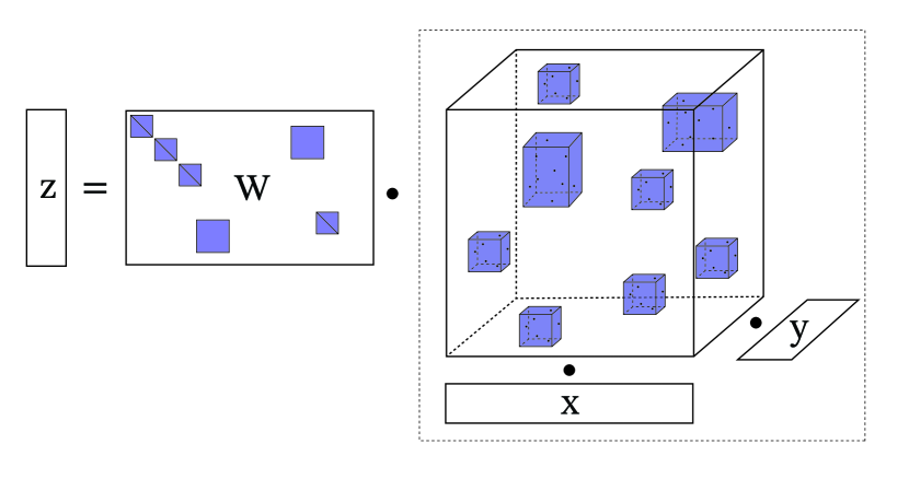
Figure 1: The CG tensor product, which contracts a block-sparse tensor $\mathcal{P}$ with two dense vectors to output a new vector. It is usually followed by multiplication with a structured weight matrix $\bm{W}$, and by convention we use “CG tensor product” to refer to both operations in sequence. Each blue block is itself sparse (see Figure 2), and several blocks may share identical structure.

A core kernel in many (though not all) rotation equivariant neural networks is the Clebsch-Gordon (CG) tensor product, which combines two feature vectors in an equivariant model to produce a new vector [32]. This multilinear operation, illustrated in Figure 1, contracts a highly-structured block sparse tensor with a pair of dense input vectors, typically followed by multiplication with a structured weight matrix. It is frequently used to combine node and edge embeddings in equivariant graph neural networks, which are used for molecular energy prediction in computational chemistry [4, 2, 26] (see Figure 4). With its low arithmetic intensity and irregular computation pattern, the CG tensor product is difficult to implement efficiently in frameworks like PyTorch or JAX. Because the CG tensor product and its derivatives must be evaluated millions of times on large atomic datasets, they remain significant bottlenecks to scaling equivariant neural networks.

We introduce an open source CUDA kernel generator for the Clebsch-Gordon tensor product and its gradients. Compared to the popular e3nn package [9] that is widely used in equivariant deep learning models, we offer up to one order of magnitude improvement for both forward and backward passes. Our forward kernels also exhibit up to 2x speedup over NVIDIA’s closed-source cuEquivariance package [10] on configurations used in graph neural networks, improving to 4.5x when we fuse the tensor product with the subsequent message passing operation. Our key innovations include:

Exploiting ILP and Sparsity:

Each nonzero block of $\mathcal{P}$ in Figure 1 is a structured tensor (see Figure 2 for illustrations of the nonzero pattern). Popular codes [9, 10] fill these blocks with explicit zeros and use optimized dense linear algebra primitives to execute the tensor product, performing unnecessary work in the process. By contrast, we use Just-in-Time (JIT) compilation to generate kernels that only perform work for nonzero tensor entries, achieving significantly higher throughput as block sparsity increases (see Table 2). While previous works [18, 16] use similar fine-grained approaches to optimize kernels for each block in isolation, we achieve high throughput by JIT-compiling a single kernel for the entire sparse tensor $\mathcal{P}$. By compiling kernels optimized for an entire sequence of nonzero blocks, we exhibit a degree of instruction level parallelism and data reuse that prior approaches do not provide.

Static Analysis and Warp Parallelism:

The structure of the sparse tensor in Figure 1 is known completely at model compile-time and contains repeated blocks with identical nonzero patterns. We perform a static analysis on the block structure immediately after the equivariant model architecture is defined to generate a computation schedule that minimizes global memory traffic. We break the calculation into a series of subkernels (see Figure 3), each implemented by aggressively caching $\bm{x}$, $\bm{y}$, and $\bm{z}$ in the GPU register file.

We adopt a kernel design where each GPU warp operates on distinct pieces of coalesced data and requires no block-level synchronization (e.g. __syncthreads()). To accomplish this, each warp manages a unique portion of the shared memory pool and uses warp-level matrix multiplication primitives to multiply operands against nonzero blocks of the structured weight matrix.

Fused Graph Convolution:

We demonstrate benefits far beyond reduced kernel launch overhead by fusing the CG tensor product with a graph convolution kernel (a very common pattern [32, 4, 2]). We embed the CG tensor product and its backward pass into two algorithms for sparse-dense matrix multiplication: a simple, flexible implementation using atomic operations and a faster deterministic version using a fixup buffer. As a consequence, we achieve significant data reuse at the L2 cache level and a reduction in global memory writes.

Section 2 provides a brief introduction to equivariant neural networks, with Section 2.2 providing a precise definition and motivation for the CG tensor product. Section 3 details our strategy to generate efficient CG kernels and the design decisions that yield high performance. We validate those decisions in Section 4 on a range of benchmarks from chemical foundation models and other equivariant architectures.

2 Preliminaries and Problem Description

We denote vectors, matrices, and three-dimensional tensors in bold lowercase characters, bold uppercase characters, and script characters (e.g. $\mathcal{P}$), respectively. Our notation and description of equivariance follow Thomas et al. [32] and Lim and Nelson [24]. Let $G$ be an abstract group of transformations, and let $\bm{D}_{\textrm{in}}:G\rightarrow\mathbb{R}^{n\times n},\bm{D}_{\textrm{out}}:G\rightarrow\mathbb{R}^{m\times m}$ be a pair of representations, group homomorphisms satisfying

$$\bm{D}_{\textrm{in}}(g_{1}\cdot g_{2})=\bm{D}_{\textrm{in}}(g_{1})\cdot\bm{D}_{\textrm{in}}(g_{2})\quad\forall g_{1},g_{2}\in G,$$

and likewise for $\bm{D}_{\textrm{out}}$. A function $\bm{f}:\mathbb{R}^{n}\rightarrow\mathbb{R}^{m}$ is equivariant with respect to $\bm{D}_{\textrm{in}}$ and $\bm{D}_{\textrm{out}}$ iff

$$\bm{f}(\bm{D}_{\textrm{in}}(g)\cdot\bm{v})=\bm{D}_{\textrm{out}}(g)\cdot\bm{f}(\bm{v})\quad\forall\bm{v}\in\mathbb{R}^{n},g\in G.$$

A function is invariant if the equivariance property holds with $\bm{D}_{\textrm{out}}(g)=\bm{I}^{m\times m}$ for all $g\in G$.

In our case, $\bm{f}$ is a neural network composed of a sequence of layers, expressed as the function composition

$$\bm{f}(\bm{v})=\bm{\phi}_{N}\circ...\circ\bm{\phi}_{1}(\bm{v}).$$

Here, $\bm{D}_{\textrm{in}}$ and $\bm{D}_{\textrm{out}}$ are derived from the dataset, and the task is to fit $\bm{f}$ to a set of datapoints while maintaining equivariance to the chosen representations. Network designers accomplish this by imposing equivariance on each layer and exploiting a composition property [32]: if $\bm{\phi}_{i}$ is equivariant to input / output representations $(\bm{D}_{i},\bm{D}_{i+1})$ and $\bm{\phi}_{i+1}$ is equivariant to $(\bm{D}_{i+1},\bm{D}_{i+2})$, then $\bm{\phi}_{i+1}\circ\bm{\phi}_{i}$ is equivariant to $(\bm{D}_{i},\bm{D}_{i+2})$. These intermediate representations are selected by the network designer to maximize predictive capability.

2.1 Representations of O(3)

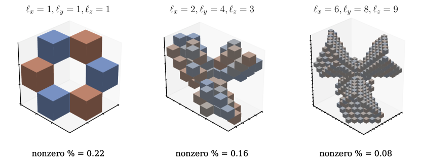
Figure 2: Three examples of CG coefficient tensors depicted by blue cubes in Figure 1. The fraction of zero entries increases with the tensor order, and the full CG tensor contains several copies of the blocks pictured here.

In this paper, we let $G=O(3)$, the group of three-dimensional rotations including reflection. A key property of real representations of $O(3)$ is our ability to block-diagonalize them into a canonical form [25]. Formally, for any representation $\bm{D}:O(3)\rightarrow\mathbb{R}^{n\times n}$ and all $g\in G$, there exists a similarity matrix $\bm{P}$ and indices $i_{1},...,i_{D}$ satisfying

$$\bm{D}(g)=\bm{P}\begin{bmatrix}\bm{D}^{(i_{1})}(g)&&0\\ &\ddots&\\ 0&&\bm{D}^{(i_{D})}(g)\end{bmatrix}\bm{P}^{-1}$$

where $\bm{D}^{(0)}(g),\bm{D}^{(1)}(g),...$ are a family of elementary, irreducible representations known as the Wigner D-matrices. For all $i\geq 0$, we have $\bm{D}^{(i)}(g)\in\mathbb{R}^{(2i+1)\times(2i+1)}$. In the models we consider, all representations will be exactly block diagonal (i.e. $\bm{P}$ is the identity matrix), described by strings of the form

$$\bm{D}(g)\cong\texttt{"3x1e + 1x2o"}.$$

This notation indicates that $D$ has three copies of $D^{(1)}$ along the diagonal followed by one copy of $D^{(2)}$. We refer to the term "3x1e" as an irrep (irreducible representation) with $\ell=1$ and multiplicity 3. The suffix letters, “e” or “o”, denote a parity used to enforce reflection equivariance, which is not relevant for us (we refer the reader to Thomas et al. [32] for a more complete explanation).

2.2 Core Computational Challenge

Let $\bm{x}\in\mathbb{R}^{n},\bm{y}\in\mathbb{R}^{m}$ be two vectors from some intermediate layer $\bm{\phi}$ of an equivariant deep neural network. For example, $\bm{x}$ could be the embedding associated with a node of a graph and $\bm{y}$ a feature vector for an edge (see Figure 4, bottom right). We can view both vectors as functions $\bm{x}(\bm{v}),\bm{y}(\bm{v})$ of the network input $\bm{v}$, which are equivariant to $(\bm{D}_{\textrm{in}},\bm{D}_{x})$ and $(\bm{D}_{\textrm{in}},\bm{D}_{y})$ respectively. An equivariant graph convolution layer $\bm{\phi}$ interacts $\bm{x}$ and $\bm{y}$ to produce a new vector $\bm{z}$. To ensure layer-equivariance of $\phi$, $\bm{z}(\bm{v})$ must be equivariant to $(\bm{D}_{\textrm{in}},\bm{D}_{z})$, where $\bm{D}_{z}$ is a new representation selected by the network designer.

The Kronecker product provides an expressive, general method to interact $\bm{x}$ and $\bm{y}$: if $\bm{x}(\bm{v})$ and $\bm{y}(\bm{v})$ are equivariant to the representations listed above, then $\bm{z}(\bm{v})=\bm{x}(\bm{v})\otimes\bm{y}(\bm{v})$ is equivariant to $(\bm{D}_{\textrm{in}},\bm{D}_{x}\otimes\bm{D}_{y})$. Unfortunately, $\bm{x}\otimes\bm{y}\in\mathbb{R}^{nm}$ may have intractable length, and we cannot drop arbitrary elements of the Kronecker product without compromising the equivariance property.

Let $\bm{P}\in\mathbb{R}^{nm\times nm}$ be the similarity transform diagonalizing $\bm{D}_{x}\otimes\bm{D}_{y}$. To reduce the dimension of the Kronecker product, we first form $\bm{P}(\bm{x}(\bm{v})\otimes\bm{y}(\bm{v}))$, which is an equivariant function with output representation $\bm{P}(\bm{D}_{x}\otimes\bm{D}_{y})\bm{P}^{-1}$. We can now safely remove segments of $\bm{P}(\bm{x}\otimes\bm{y})$ corresponding to unneeded higher-order Wigner blocks and recombine its components through a trainable, structured weight matrix. The result, $\bm{z}(\bm{v})=\bm{W}\bm{P}(\bm{x}(\bm{v})\otimes\bm{y}(\bm{v}))$, has a new output representation $\bm{D}_{z}$ and can be much shorter than $\bm{x}\otimes\bm{y}$.

When both $\bm{D}_{x}$ and $\bm{D}_{y}$ are representations in block-diagonal canonical form, the transform $\bm{P}$ is a highly structured block-sparse matrix containing nonzero Clebsch-Gordon coefficients. After potentially reducing $\bm{P}$ to $k$ rows (removing segments corresponding to unneeded Wigner D-blocks), we can reshape it into a block-sparse tensor $\mathcal{P}\in\mathbb{R}^{m\times n\times k}$ contracted on two sides with $\bm{x}$ and $\bm{y}$. We call this operation (along with multiplication by a structured weight matrix $\bm{W}\in\mathbb{R}^{k\times k^{\prime}}$) the CG tensor product, illustrated in Figure 1. It can be expressed by a matrix equation, a summation expression, multilinear tensor contraction (popular in the numerical linear algebra community), or Einstein notation:

(2.1) $$\bm{z} =\boxed{\textrm{TP}(\mathcal{P},\bm{x},\bm{y},\bm{W})}$$

$$:=\bm{W}\cdot\bm{P}\cdot(\bm{x}\otimes\bm{y})$$

$$:=\bm{W}\sum_{i=1,j=1}^{m,n}\bm{x}\left[i\right]\bm{y}\left[j\right]\mathcal{P}\left[ij:\right]$$

$$:=\mathcal{P}\times_{1}\bm{x}\times_{2}\bm{y}\times_{3}\bm{W}$$

$$:=\textrm{einsum}(``ijk,i,j,kk^{\prime}\rightarrow k^{\prime}",\mathcal{P},\bm{x},\bm{y},\bm{W}).$$

Our goal is to accelerate computation of $\textrm{TP}(\mathcal{P},\bm{x},\bm{y},\bm{W})$ for a variety of CG coefficient tensors $\mathcal{P}$. Given $\partial E/\partial\bm{z}$ for some scalar quantity $E$, we will also provide an efficient kernel to compute $\partial E/\partial\bm{x}$, $\partial E/\partial\bm{y}$, and $\partial E/\partial\bm{W}$ in a single pass. These gradients are required during both training and inference for some interatomic potential models.

2.3 Structure in the Sparse Tensor and Weights

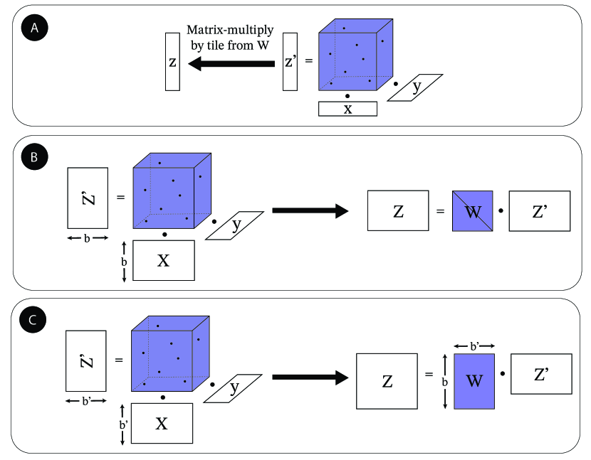
Figure 3: Fundamental subkernels that compose to implement the CG tensor product in Figure 1. In (A), $\bm{x}$, $\bm{y}$, and $\bm{z}$ refer to segments of the longer vectors in Figure 1, and $\bm{W}$ contains entries from the larger weight matrix rearranged appropriately. In (B) and (C), $\bm{X}$ and $\bm{Z}$ refer to segments from $\bm{x}$ and $\bm{z}$ that have been reshaped into matrices to exploit repeating sparse tensor structure. $b$ and $b^{\prime}$ are multiples of 32 in many models.

Suppose $\bm{D}_{x}$, $\bm{D}_{y}$, and $\bm{D}_{z}$ each consist of a single Wigner block. In this case, the tensor $\mathcal{P}$ in Figure 1 has a single nonzero block of dimensions $(2\ell_{x}+1)\times(2\ell_{y}+1)\times(2\ell_{z}+1)$. Figure 2 illustrates three blocks with varying parameters, which are small, (current models typically use $\ell_{x},\ell_{y},\ell_{z}\leq 4$), highly structured, and sparse.

Every nonzero block of the general tensor $\mathcal{P}$ in Figure 1 takes the form $\mathcal{P}^{(\ell_{x},\ell_{y},\ell_{z})}$. Therefore, we could implement the CG tensor product by repeatedly calling the kernel in Figure 3A: a small tensor contraction followed by multiplication by a tile from the weight matrix $\bm{W}$. In practice, this is an inefficient strategy because $\mathcal{P}$ may contain hundreds of blocks with identical nonzero structures and values.

Instead, the CG tensor product splits into a sequence of subkernels [18] that match the structure in $\mathcal{P}$ and $\bm{W}$. We target two common patterns. First, the CG tensor product may interact $b$ unique segments of $\bm{x}$ with a common segment of $\bm{y}$ using the same CG sparse tensor, followed by multiplication by a submatrix of weights from $\bm{W}$ rearranged along a diagonal. Figure 3B illustrates this primitive as a contraction of a sparse tensor with a matrix $\bm{X}$ (containing the $b$ rearranged segments from $\bm{x}$) and the common vector $\bm{y}$. It appears in the Nequip [4] and MACE [2] models. Kernel C is identical to kernel B, but arranges the weights in a dense matrix $\bm{W}\in\mathbb{R}^{b^{\prime}\times b}$; the row count of $\bm{Z}$ may be distinct from the row count of $\bm{X}$. The latter operation appears in DiffDock [6] and 3D shape classifiers by Thomas et al. [32]. Both operations can be extended to interact multiple segments from $\bm{y}$, but we could not find this pattern in existing equivariant models. While kernels besides B and C are possible, they rarely appear in practice.

2.4 A Full Problem Description

Armed with the prior exposition, we now give an example of a specific CG tensor product using the notation of the e3nn software package [9]. A specification of the tensor product consists of a sequence of subkernels and the representations that partition $\bm{x}$, $\bm{y}$, and $\bm{z}$ into segments for those kernels to operate on:

(2.2) $$\bm{D}_{x}\cong\texttt{32x2e + 32x1e}$$

$$\bm{D}_{y}\cong\texttt{1x3e + 1x1e}$$

$$\bm{D}_{z}\cong\texttt{32x5e + 16x2e + 32x3e}$$

$$\left[(1,1,1,``B"),(1,2,2,``C"),(1,2,3,``C")\right].$$

Here, $\bm{x}$ and $\bm{y}$ are partitioned into two segments, while $\bm{z}$ is partitioned into three segments. The list of tuples on the last line specifies the subkernels to execute and the segments they operate on. The first list entry specifies kernel B with the respective first segments of $\bm{x}$, $\bm{y}$, and $\bm{z}$ ($b=32$). Likewise, the second instruction executes kernel C with the first segment of $\bm{x}$ and the second segment of $\bm{y}$ ($b^{\prime}=32,b=16$) to produce the second segment of $\bm{z}$.

2.5 Context and Related Work

Variants of rotation equivariant convolutional neural networks were first proposed by Weiler et al. [34]; Kondor et al. [19]; and Thomas et al. [32]. Nequip [4], Cormorant [1], and Allegro [26] deploy equivariant graph neural networks to achieve state-of-the-art performance for molecular energy prediction. Other works have enhanced these message-passing architectures by adding higher-order equivariant features (e.g. MACE [2, 3] or ChargE3Net [17]). Equivariance has been integrated into transformer architectures [7, 23] with similar success.

Equivariant Deep Learning Software

The e3nn package [8, 9] allows users to construct CG interaction tensors, compute CG tensor products, explicitly form Wigner D-matrices, and evaluate spherical harmonic basis functions. PyTorch and JAX versions of the package are available. The e3x package [33] offers similar functionality. Allegro [26] modifies the message passing equivariant architecture in Nequip [4] to drastically reduce the number of CG tensor products and lower inter-GPU communication.

The cuEquivariance package [10], released by NVIDIA concurrent to this project’s development, offers the fastest implementation of the CG tensor product outside of our work. However, their kernels are closed-source and do not appear to exploit sparsity within each nonzero block of $\mathcal{P}$. Our kernel performance matches or exceeds cuEquivariance, often by substantial margins. Related codes include the GELib library [18] and Equitriton [22], the former to efficiently compute tensor products and the latter to evaluate spherical harmonic polynomials. Although GELib is less widely used in production models, we analyze its custom CUDA kernels in Section 3.6.

Alternatives to CG Contraction

The intense cost of the CG tensor product has fueled the search for cheaper yet accurate algorithms. For example, Schütt et al. [29] propose an equivariant message passing neural network that operates in Cartesian space, eliminating the need for CG tensor products. Luo et al. [25] connect the tensor product with a spherical harmonic product accelerated through the fast Fourier transform, an operation they call the Gaunt tensor product. Xie et al. [36] counter that the Gaunt tensor product does not produce results directly comparable to the CG tensor product, and that the former may sacrifice model expressivity. Lee et al. [21] observe that higher-order equivariant features may not improve model performance, while Qu and Krishnapriyan [28] achieve high accuracy by altogether eliminating hard rotational constraints in interatomic potential models.

GPU Architecture

GPUs execute kernels by launching a large number of parallel threads running the same program, each accessing a small set of local registers. In a typical program, threads load data from global memory, perform computation with data in their registers, and store back results. Kernels are most efficient when groups of 32-64 threads (called “warps”) execute the same instruction or perform memory transaction on contiguous, aligned segments of data. Warps execute asynchronously and are grouped into cooperative thread arrays (CTAs, called blocks in CUDA), which can communicate through a fast, limited pool of shared memory. Warps can synchronize at the CTA level, but the synchronization incurs overhead.

3 Engineering Efficient CG Kernels

Our task is to generate an efficient CG tensor product kernel given a problem specification outlined in Section 2.4. Algorithm 1 describes the logic of a kernel that operates on a large batch of inputs, each with a distinct set of weights (see Figure 4B). We assign each $(\bm{x},\bm{y},\bm{W})$ input triple to a single GPU warp, a choice which has two consequences. First, it enables each warp to execute contiguous global memory reads / writes for $\bm{x},\bm{y},\bm{W}$ and $\bm{z}$. Second, it allows warps to execute in a completely asynchronous fashion without any CTA-level synchronization, boosting throughput significantly. The weights $\bm{W}$ are stored in a compressed form without the zero entries illustrated in Figure 1.

After the division of labor, each warp follows a standard GPU kernel workflow. The three inputs are staged in shared memory, the kernels in Equation (2.2) are executed sequentially, and each output $\bm{z}_{b}$ is stored back. Each warp operates on a unique partition of the CTA shared memory which may not be large enough to contain the the inputs and outputs. In the latter case, chunks of $\bm{x}$, $\bm{y}$, $\bm{W}$, and $\bm{z}$ are staged, and the computation executes in phases according to a schedule described in Section 3.1.

Algorithm 1 High-Level CGTP Algorithm

Batch $\bm{x}_{1}...\bm{x}_{B}$, $\bm{y}_{1}...\bm{y}_{B}$,$\bm{W}_{1}...\bm{W}_{B}$

for $b=1...B$ do $\triangleright$ Parallel over warps

  for $\textrm{seg}_{i}\in\textrm{schedule}$ do

   Load $\bm{x}_{\textrm{smem}}=\bm{x}_{b}\left[\textrm{seg}_{i\ \textrm{(x start)}}:\textrm{seg}_{i\ \textrm{(x end)}}\right]$

   Load $\bm{y}_{\textrm{smem}},\bm{W}_{\textrm{smem}}$ similarly.

   Set $\bm{z}_{\textrm{smem}}=0$

   for $\textrm{kern}_{j}\in\textrm{seg}_{i}$ do

     Set $\bm{X}_{\textrm{kern}}$ as a reshaped range of $\bm{x}_{\textrm{smem}}$

     Set $\bm{y}_{\textrm{kern}},\bm{W}_{\textrm{kern}}$ similarly.

     $\bm{Z}_{\textrm{kern}}=\textrm{kern}_{j}(\bm{X}_{\textrm{kern}},\bm{y}_{\textrm{kern}},\bm{W}_{\textrm{kern}})$

     Flatten, store $\bm{Z}_{\textrm{kern}}$ to subrange of $\bm{z}_{\textrm{smem}}$

   end for

   Store $\bm{z}_{b}\left[\textrm{seg}_{i\ \textrm{(z start)}}:\textrm{seg}_{i\ \textrm{(z end)}}\right]\mathrel{{+}}=\bm{z}_{\textrm{smem}}$

  end for

end for

We launch a number of CTAs that is a constant multiple of the GPU streaming multiprocessor count and assign 4-8 warps per CTA. The batch size for the CG tensor product can reach millions [26] for large geometric configurations, ensuring that all warps are busy. The computation required for each batch element can exceed 100K FLOPs for typical models [26, 4], ensuring that the threads within each warp are saturated with work.

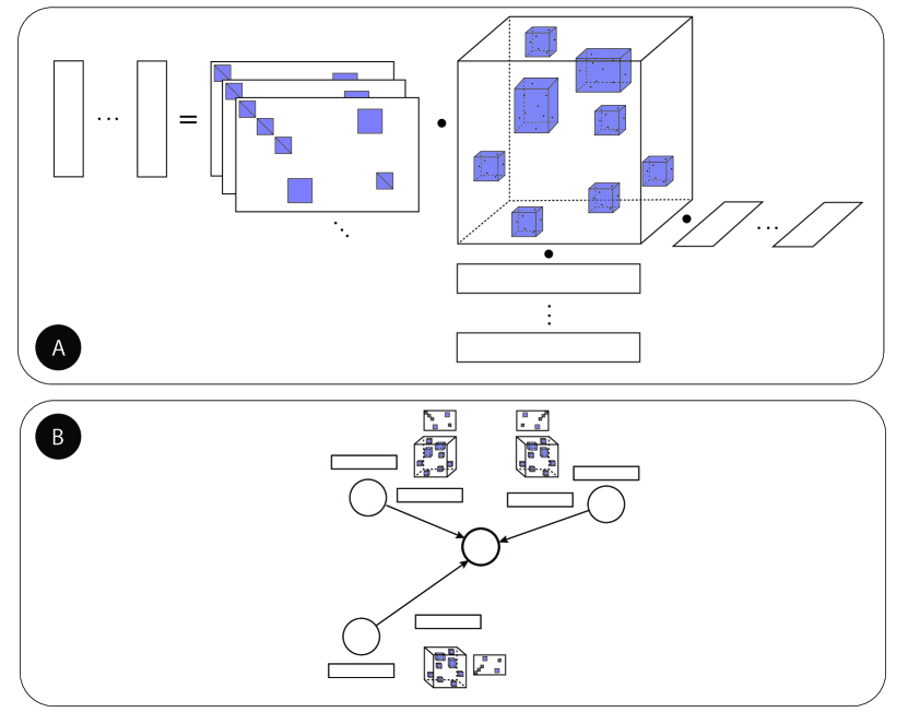
Figure 4: Applications of the CG tensor product. The simplest and most general use case (A) calls the kernel repeatedly with distinct $\bm{x}$, $\bm{y}$, and $\bm{W}$ inputs. Interatomic potential models embed the operation in a graph convolution (B), where the tensor product combines node features with edge features.

3.1 Computation Scheduling

A key obstacle to efficient kernel implementation is the long length of the $\bm{x}$, $\bm{y}$, and $\bm{z}$ feature vectors that must be cached in shared memory. The sum of their vector lengths for large MACE [3] and Nequip [4] configurations can exceed 10,000 data words. Given that the warps in each CTA partition the shared memory, staging all three vectors at once (along with the weights in $\bm{W}$) is infeasible.

To manage our limited shared memory, we execute the computation in phases that are scheduled at model compile-time. We break the list of instructions in Equation (2.2) into phases so that the sum of chunks from $\bm{x}$, $\bm{y}$, $\bm{W}$ and $\bm{z}$ required for the phase fits in each warp’s shared memory allotment. We then schedule loads and stores, hardcoding the relevant instructions into each kernel using our JIT capability. When more than a single computation phase is required, our goal is to generate a schedule that minimizes global memory reads and writes. We use a few simple heuristics:

1. If $\bm{x}$ and $\bm{y}$ can fit into a warp’s shared memory partition (but not $\bm{z}$ and $\bm{W}$), then segments of $\bm{z}$ and $\bm{W}$ are streamed in through multiple phases of computation. In each phase, the kernels that touch each segment of $\bm{z}$ are executed.

2. Otherwise, we use a greedy algorithm. In each phase, the shared memory pool is filled with as many segments of $\bm{x}$, $\bm{y}$, $\bm{W}$ and $\bm{z}$ that can fit. Between phases, segments are flushed and reloaded as needed.

Case 1 covers most problem configurations in equivariant graph neural networks and minimizes global memory writes, while Case 2 enables reasonable performance even with constrained shared memory resources. Large CG tensors (e.g. Nequip-benzene in Figure 5) may require 20-40 phases of computation per tensor product, and our scheduling substantially reduces global memory transactions.

3.2 JIT Subkernel Implementations

In preparation to execute a subkernel, suppose we have loaded $\bm{x}$, $\bm{y}$ and $\bm{W}$ into shared memory and reshaped subranges of all three to form $\bm{X}_{\textrm{kern}},\bm{y}_{\textrm{kern}}$, and $\bm{W}_{\textrm{kern}}$. For the rest of Section 3.2 and all of Section 3.3, we omit the “kern” subscripts. Algorithm 2 gives the pseudocode to execute either kernel B or C from Figure 3 using these staged operands.

Algorithm 2 Subkernel B & C Warp-Level Algorithm

$\bm{X}\in\mathbb{R}^{b^{\prime}\times(2\ell_{x}+1)},\bm{y}\in\mathbb{R}^{(2\ell_{y}+1)},\bm{W}\in\mathbb{R}^{b\times b^{\prime}}$

Sparse tensor $\mathcal{P}^{(\ell_{x},\ell_{y},\ell_{z})}$ for subkernel

for $t=1...b^{\prime}$ do $\triangleright$ Parallel over threads

  Load $\bm{x}_{\textrm{reg}}=\bm{X}\left[t,:\right]$, $\bm{y}_{\textrm{reg}}=\bm{y}$

  Initialize $\bm{z}_{\textrm{reg}}\in\mathbb{R}^{2\ell_{z}+1}$ to 0.

  

  for $(i,j,k,v)\in\textrm{nz}(\mathcal{P})$ do $\triangleright$ Unroll via JIT

   $\bm{z}_{\textrm{reg}}\left[k\right]\mathrel{{+}}=v\cdot\bm{x}_{\textrm{reg}}\left[i\right]\cdot\bm{y}_{\textrm{reg}}\left[j\right]$

  end for

  

  if $\bm{W}$ is diagonal then $\triangleright$ Compile-time branch

   $\bm{Z}\left[t,:\right]\mathrel{{+}}=\bm{W}\left[t,t\right]\cdot\bm{z}_{\textrm{reg}}$

  else

   Store $\bm{Z}^{\prime}\left[t,:\right]=\bm{z}_{\textrm{reg}}$, compute $\bm{Z}\mathrel{{+}}=\bm{W}\cdot\bm{Z}^{\prime}$

  end if

end for

Each thread stages a unique row row of $\bm{X}$ and $\bm{Z}$, as well as the entirety of $\bm{y}$, into its local registers. Models such as Nequip [4] and MACE [3] satisfy $\ell_{x},\ell_{y},\ell_{z}\leq 4$, so the added register pressure from the operand caching is manageable. We then loop over all nonzero entries of the sparse tensor to execute the tensor contraction. Because the nonzero indices $(i,j,k)$ and entries $\bm{v}$ of the sparse tensor $\mathcal{P}$ are known at compile-time, we emit the sequence of instructions in the inner loop explicitly using our JIT kernel generator. Finally, the output $\bm{Z}$ is accumulated to shared memory after multiplication by $\bm{W}$. When multiple subkernels execute in sequence, we allow values in $\bm{x}_{\textrm{reg}}$, $\bm{y}_{\textrm{reg}}$, and $\bm{z}_{\textrm{reg}}$ to persist if they are reused.

The matrix multiplication by the weights at the end of Algorithm 2 depends on the structure of $\bm{W}$. When $\bm{W}$ is square and diagonal (kernel B), multiplication proceeds asynchronously in parallel across all threads. When $\bm{W}$ is a general dense matrix, we temporarily store $\bm{z}_{\textrm{reg}}$ to shared memory and perform a warp-level matrix-multiplication across all threads. Our final implementation uses a mix of hand-rolled kernels and CUTLASS [31] for warp matrix multiplication.

Our kernel generator maximizes instruction-level parallelism, and the output kernels contain long streams of independent arithmetic operations. By contrast, common sparse tensor storage formats (coordinate [11], compressed-sparse fiber [30], etc.) require expensive memory indirections that reduce throughput. Because we compile a single kernel to handle all nonzero blocks of $\mathcal{P}$, we avoid expensive runtime branches and permit data reuse at the shared memory and register level. Such optimizations would be difficult to implement in a traditional statically-compiled library.

For typical applications, $b$ and $b^{\prime}$ are multiples of 32. When $b$ is greater than 32, the static analysis algorithm in Section 3.1 breaks the computation into multiple subkernels with $b\leq 32$, and likewise for $b^{\prime}$.

3.3 Backward Pass

Like other kernels in physics informed deep learning models [15], the gradients of the CG tensor product are required during model inference as well as training for interatomic force prediction. Suppose $E(\bm{R},\bm{W})$ is the scalar energy prediction emitted by our equivariant model for a configuration of $s$ atoms, where $\bm{W}$ contains trainable model weights and each row of $\bm{R}\in\mathbb{R}^{s\times 3}$ is an atom coordinate. Then $\bm{F}_{\textrm{pr}}=-\partial E/\partial\bm{R}\in\mathbb{R}^{s\times 3}$ is the predicted force on each atom. Conveniently, we can compute these forces by auto-differentiating $E(\bm{R},\bm{W})$ in a framework like PyTorch or JAX, but we require a kernel to compute the gradient of the CG tensor product inputs given the gradient of its output.

To implement the backward pass, suppose $\bm{z}=\textrm{TP}(\mathcal{P},\bm{x},\bm{y},\bm{W})$ and we have $\bm{g}_{z}=\partial E/\partial\bm{z}$. Because the CG tensor product is linear in its inputs, the product rule gives

$$\partial E/\partial\bm{x}\left[i\right] =\sum_{(i,j,k)\in\textrm{nz}(\mathcal{P})}\mathcal{P}\left[ijk\right]\cdot\bm{y}\left[j\right]\cdot\left(\bm{W}^{\top}\cdot\bm{g}_{z}\right)\left[k\right]$$

$$\partial E/\partial\bm{y}\left[j\right] =\sum_{(i,j,k)\in\textrm{nz}(\mathcal{P})}\mathcal{P}\left[ijk\right]\cdot\bm{x}\left[i\right]\cdot\left(\bm{W}^{\top}\cdot\bm{g}_{z}\right)\left[k\right]$$

$$\partial E/\partial\bm{W}\left[kk^{\prime}\right] =\bm{g}_{z}\left[k^{\prime}\right]\cdot\sum_{(i,j,k)\in\textrm{nz}(\mathcal{P})}\mathcal{P}\left[ijk\right]\bm{x}\left[i\right]\bm{y}\left[j\right]$$

Notice the similarity between the three equations above and Equation (2.1): all require summation over the nonzero indices of $\mathcal{P}$ and multiplying each value with a pair of elements from distinct vectors. Accordingly, we develop Algorithm 3 with similar structure to Algorithm 2 to compute all three gradients in a single kernel. For simplicity, we list the general case where the submatrix $\bm{W}$ is a general dense matrix (kernel C).

Algorithm 3 Subkernel C Warp-Level Backward

$\bm{X}\in\mathbb{R}^{b^{\prime}\times(2\ell_{x}+1)},\bm{y}\in\mathbb{R}^{2\ell_{y}+1},\bm{W}\in\mathbb{R}^{b\times b^{\prime}}$

$\bm{G}_{Z}\in\mathbb{R}^{b\times(2\ell_{z}+1)}$, sparse tensor $\mathcal{P}^{(\ell_{x},\ell_{y},\ell_{z})}$

Threads collaboratively compute $\bm{G}_{Z}^{\prime}=\bm{W}^{\top}\cdot\bm{G}_{Z}$

for $t=1...b^{\prime}$ do $\triangleright$ Parallel over threads

  Load $\bm{x}_{\textrm{reg}}=\bm{X}\left[t,:\right]$, $\bm{y}_{\textrm{reg}}=\bm{y}$, $\bm{g}_{z\textrm{reg}}^{\prime}=\bm{G}_{Z}^{\prime}\left[t:\right]$

  Initialize $\bm{g}_{\textrm{x reg}},\bm{g}_{\textrm{y reg}},\bm{g}_{\textrm{w reg}},\bm{z}_{\textrm{reg}}$ to 0.

  

  for $(i,j,k,v)\in\textrm{nz}(\mathcal{P}^{(\ell_{x},\ell_{y},\ell_{z})}$ do $\triangleright$ Unroll via JIT

   $\bm{g}_{\textrm{x reg}}\left[i\right]\mathrel{{+}}=v\cdot\bm{y}_{\textrm{reg}}\left[j\right]\cdot\bm{g}_{\textrm{z reg}}^{\prime}\left[k\right]$

   $\bm{g}_{\textrm{y reg}}\left[j\right]\mathrel{{+}}=v\cdot\bm{x}_{\textrm{reg}}\left[i\right]\cdot\bm{g}_{\textrm{z reg}}^{\prime}\left[k\right]$

   $\bm{z}_{\textrm{reg}}\left[k\right]\mathrel{{+}}=v\cdot\bm{x}_{\textrm{reg}}\left[i\right]\cdot\bm{y}_{\textrm{reg}}\left[j\right]$

  end for

  

  Store $\bm{g}_{y}=\textrm{warp-reduce}(\bm{g}_{\textrm{y reg}})$

  Store $\bm{G}_{x}\left[t,:\right]=\bm{g}_{\textrm{x reg}}$ and $\bm{Z}^{\prime}\left[t,:\right]=\bm{z}_{\textrm{reg}}$

end for

Threads collaboratively compute $G_{W}=\bm{G}_{Z}\cdot(\bm{Z}^{\prime})^{\top}$

There are two new key features in Algorithm 3: first, we must perform a reduction over the warp for the gradient vector $\bm{g}_{y}$, since each thread calculates a contribution that must be summed. Second: when $\bm{W}$ is not diagonal, an additional warp-level matrix multiply is required at the end of the algorithm to calculate $\bm{G}_{W}$. We embed Algorithm 3 into a high-level procedure akin to Algorithm 1 to complete the backward pass.

3.4 Higher Partial Derivatives

Our analysis so far has focused on the forward and backward passes for the CG tensor product. For interatomic potential models, we require higher-order derivatives to optimize force predictions during training [15], as we explain below. Rather than write new kernels for these derivatives, we provide a novel (to the best of our knowledge) calculation that implements them using the existing forward and backward pass kernels.

As in Section 3.3, let $\bm{F}_{\textrm{pr}}=-\partial E/\partial\bm{R}\in\mathbb{R}^{s\times 3}$ be the predicted atomic forces generated by our model. During training, we must minimize a loss function of the form

$$\min_{\bm{W}}\mathcal{L}(\bm{R},\bm{W})=\min_{\bm{W}}\left\lVert\bm{F}_{\textrm{pr}}(\bm{R},\bm{W})-\bm{F}_{\textrm{gt}}(\bm{R})\right\rVert_{F}^{2}$$

where $\bm{F}_{\textrm{gt}}(\bm{R})\in\mathbb{R}^{s\times 3}$ is a set of ground-truth forces created from a more expensive simulation. The loss function may include other terms, but only the Frobenius norm of the force difference is relevant here. We use a gradient method to perform the minimization and calculate

(3.3) $$\frac{\partial\mathcal{L}}{\partial\bm{W}} =2\cdot\textrm{vec}(\bm{F}_{\textrm{pr}}(\bm{R},\bm{W})-\bm{F}_{\textrm{gt}}(\bm{R}))^{\top}\frac{\partial\bm{F}_{\textrm{pr}}}{\partial\bm{W}}$$

$$=-2\cdot\textrm{vec}(\bm{F}_{\textrm{pr}}(\bm{R},\bm{W})-\bm{F}_{\textrm{gt}}(\bm{R}))^{\top}\frac{\partial^{2}E}{\partial\bm{R}\partial\bm{W}}$$

where “vec” flattens its matrix argument into a vector and $\partial^{2}E/(\partial\bm{R}\partial\bm{W})\in\mathbb{R}^{3s\times(\textrm{\# weights})}$ is a matrix of second partial derivatives. Equation (3.3) can also be computed by auto-differentiation, but the second partial derivative requires us to register an autograd formula for our CG tensor product backward kernel (i.e. we must provide a “double-backward” implementation).

To avoid spiraling engineering complexity, we will implement the double-backward pass by linearly combining the outputs from existing kernels. Let $\bm{z}=\textrm{TP}(\bm{x},\bm{y},\bm{W})$ (we omit the sparse tensor argument $\mathcal{P}$ here) and define $\bm{g}_{z}=\partial E/\partial\bm{z}$ for the scalar energy prediction $E$. Finally, let $\bm{a}$, $\bm{b}$, and $\bm{C}$ be the gradients calculated by the backward pass, given as

$$\left[\bm{a},\bm{b},\bm{C}\right] =\left[\partial E/\partial\bm{x},\partial E/\partial\bm{y},\partial E/\partial\bm{W}\right]$$

$$=\textrm{backward}\left(\bm{x},\bm{y},\bm{W},\bm{g}_{z}\right).$$

Now our task is to compute ($\partial\mathcal{L}/\partial\bm{x}$, $\partial\mathcal{L}/\partial\bm{y}$, $\partial\mathcal{L}/\partial\bm{W}$, $\partial\mathcal{L}/\partial\bm{g}_{z}$) given ($\partial\mathcal{L}/\partial\bm{a}$, $\partial\mathcal{L}/\partial\bm{b}$, $\partial\mathcal{L}/\partial\bm{C}$). We dispatch seven calls to the forward and backward pass kernels:

(3.4) op1 $$=\textrm{backward}(\bm{a},\bm{b},\bm{W},\bm{g}_{z})$$

op2 $$=\textrm{backward}(\bm{x},\bm{y},\bm{C},\bm{g}_{z})$$

op3 $$=\textrm{TP}(\bm{a},\bm{y},\bm{W})$$

op4 $$=\textrm{backward}(\bm{a},\bm{y},\bm{W},\bm{g}_{z})$$

op5 $$=\textrm{backward}(\bm{x},\bm{b},\bm{W},\bm{g}_{z})$$

op6 $$=\textrm{TP}(\bm{x},\bm{b},\bm{W})$$

op7 $$=\textrm{TP}(\bm{x},\bm{y},\bm{C}).$$

By repeatedly applying the product and chain rules to the formulas for $a$, $b$, and $c$ in Section 3.3, we can show

(3.5) $$\partial\mathcal{L}/\partial\bm{x} =\textrm{op1}\left[1\right]+\textrm{op2}\left[1\right]$$

$$\partial\mathcal{L}/\partial\bm{y} =\textrm{op1}\left[2\right]+\textrm{op2}\left[2\right]$$

$$\partial\mathcal{L}/\partial\bm{W} =\textrm{op4}\left[3\right]+\textrm{op5}\left[3\right]$$

$$\partial\mathcal{L}/\partial\bm{g}_{z} =\textrm{op3}+\textrm{op6}+\textrm{op7},$$

where $\textrm{op1}\left[1\right]$, $\textrm{op1}\left[2\right]$, and $\textrm{op2}\left[3\right]$ denote the three outputs calculated by the backward pass, and likewise for op4 and op5. Equations (3.4) and (3.5) can be implemented in less than 10 lines of Python and accelerate the double-backward pass without any additional kernel engineering. We checked the correctness of our double-backward implementation against e3nn, which computes the quantities in Equation (3.5) automatically (albeit slowly) through autodifferentation.

Our approach offers several additional advantages. Equations (3.4) and (3.5) are agnostic to the structure of $\mathcal{P}$, rendering the double-backward algorithm correct as long as the associated forward and backward kernels are correct. Because Equation (3.4) recursively calls operations with registered autograd formulas, an autograd framework can compute arbitrary higher partial derivatives of our model, not just double-backward. Finally, these formulas continue to apply when the CG tensor product is embedded within a graph convolution (see Section 3.5), composing seamlessly with the other optimizations we introduce.

3.5 Graph Convolution and Kernel Fusion

Figure 4 illustrates two typical use cases of the CG tensor product kernel. The first case (4A) calls the kernel illustrated in Figure 1 several times with unique triples of $(\bm{x},\bm{y},\bm{W})$ inputs, and we have already addressed its implementation. The second case (4B) embeds the CG tensor product into a graph convolution operation [32, 4, 2]. Here, the nodes of a graph typically correspond to atoms in a simulation and edges represent pairwise interactions. For a graph $G=(V,E)$, let $\bm{x}_{1}...\bm{x}_{\left|V\right|}$ $\bm{y}_{1}...\bm{y}_{\left|E\right|}$, and $\bm{W}_{1}...\bm{W}_{\left|E\right|}$ be node embeddings, edge embeddings, and trainable edge weights, respectively. Then each row $\bm{z}_{j}$ of the graph convolution output, $j\in\left[\left|V\right|\right]$, is given by

(3.6) $$\bm{z}_{j}=\sum_{(j,k,e)\in\mathcal{N}(j)}\textrm{TP}(\mathcal{P},\bm{x}_{k},\bm{y}_{e},\bm{W}_{e}),$$

where $\mathcal{N}(j)$ denotes the neighbor set of node $j$ and $(j,k,e)\in\mathcal{N}(j)$ indicates that edge $e$ connects nodes $j$ and $k$. Current equivariant message passing networks [4, 2] implement Equation (3.6) by duplicating the node features to form $\bm{x}_{1}^{\prime},...,\bm{x}_{\left|E\right|}^{\prime}$, calling the large batch kernel developed earlier, and then executing a scatter-sum (also called reduce-by-key) to perform aggregation. Unfortunately, duplicating the node features incurs significant memory and communication-bandwidth overhead when $\left|E\right|\gg\left|V\right|$ (see Table 3).

Notice that graph convolution exhibits a memory access pattern similar to sparse-dense matrix multiplication (SpMM) [37]. We provide two procedures for the fused CGTP / graph convolution based on classic SpMM methods. The first, detailed in Algorithm 4, requires row-major sorted edge indices and iterates over the phases of the computation schedule as the outer loop. The latter change enables the algorithm to keep a running buffer $\bm{z}_{\textrm{acc}}$ that accumulates the summation in Equation (3.6) for each node. The buffer $\bm{z}_{\textrm{acc}}$ is only flushed to global memory when a warp transitions to a new row of the graph adjacency matrix, reducing global memory writes from $O(\left|E\right|)$ to $O(\left|V\right|)$. To handle the case where two or more warps calculate contributions to the same node, we write the first row processed by each warp to a fixup buffer [37]. We developed a backward pass kernel using a similar SpMM strategy, but a permutation that transposes the graph adjacency matrix is required as part of the input.

Algorithm 4 Deterministic TP + Graph Convolution

Graph $G=(V,E)$, $E\left[b\right]=(i_{b},j_{b})$

Edges in $E$ sorted by first coordinate.

Batch $\bm{x}_{1},...,\bm{x}_{\left|V\right|}$, $\bm{y}_{1},...\bm{y}_{\left|E\right|}$,$\bm{W}_{1},...,\bm{W}_{\left|E\right|}$

for $\textrm{seg}_{i}\in\textrm{schedule}$ do

  $(s,t)=E\left[k\right]\left[0\right],E\left[k\right]\left[1\right]$

  Set $\bm{z}_{\textrm{acc}}=0$

  for $b=1...\left|E\right|$ do $\triangleright$ Parallel over warps

   $\bm{x}_{\textrm{smem}}=\bm{x}_{t}\left[\textrm{seg}_{i\ \textrm{(x start)}}:\textrm{seg}_{i\ \textrm{(x end)}}\right]$

   Load $\bm{y}_{\textrm{smem}},\bm{W}_{\textrm{smem}}$ similarly, set $\bm{z}_{\textrm{smem}}=0$.

   Run kernels as in Algorithm 1.

   $\bm{z}_{\textrm{acc}}\mathrel{{+}}=\bm{z}_{\textrm{smem}}$

   if $b=\left|E\right|$ or $s<E\left[b+1\right]\left[0\right]$ then

     if $s$ is first vertex processed by warp then

      Send $\bm{z}_{\textrm{acc}}$ to fixup buffer.

     else

      $\bm{z}_{s}\left[\textrm{seg}_{i\ \textrm{(z start)}}:\textrm{seg}_{i\ \textrm{(z end)}}\right]\mathrel{{+}}=\bm{z}_{\textrm{acc}}$

     end if

     $\bm{z}_{\textrm{acc}}=0$

   end if

  end for

end for

Execute fixup kernel.

The second algorithm, which we omit for brevity, functions almost identically to Algorithm 4, but replaces the fixup / store logic with an atomic accumulation at every inner loop iteration. This method performs $O(\left|E\right|)$ atomic storebacks, but does not require a sorted input graph or adjacency transpose permutation. Figure 8 shows that the atomic algorithm still benefits from increased temporal L2 cache locality induced by the graph.

3.6 Analysis and Related Work Comparison

Our JIT-based approach embeds the sparse tensor structure and values into the GPU instruction stream, which is only possible because $\mathcal{P}$ has relatively few nonzero entries in each block. Because GPU instructions must also be fetched from global memory, performance eventually degrades as blocks exceed several thousand nonzero entries. We do not encounter such tensors in practical models.

Kondor et al. [19] used the GElib library [18] to implement one of the original $\textrm{O}(3)$-equivariant deep learning models. Their library also employs fine-grained loop unrolling in CUDA and parallelizes distinct tensor product evaluations across threads. Despite these strong innovations, their statically compiled library does not provide an optimized backward pass, synchronizes at the CTA rather than warp level, and handles each nonzero block of $\mathcal{P}$ with a separate kernel invocation. GElib does not match the performance of e3nn and faces obstacles to data reuse, which we overcome through our computation schedule and JIT compilation.

4 Experiments

Our kernel generator is available online. We adopted the frontend interface of e3nn [8, 9] and used QuTiP [13, 20] to generate CG coefficients; we thank the authors of both packages. We tested correctness against e3nn to ensure that our kernels produce identical results, up to floating point roundoff and a well-defined reordering of the weights $\bm{W}$ on certain input configurations.

Experiments were conducted on NVIDIA A100 GPU nodes of NERSC Perlmutter (each equipped with an AMD EPYC 7763 CPU). Table 1 lists the advertised maximum memory bandwidth and compute peaks for multiple datatypes, a yardstick for our results.

Quantity	Value
FP32 Peak	19.5 TFLOP/s
FP64 SIMT Peak	9.7 TFLOP/s
FP64 Tensor Core Peak	19.5 TFLOP/s
HBM2 Bandwidth	2.04 TBP/s

Table 1: A100-SXM4-80GB performance [5].

As baselines, we used the PyTorch versions of e3nn (v0.5.4) [9] and NVIDIA cuEquivariance (v0.0.2) [10]. The e3nn implementation was accelerated with torch.compile except where prohibited by memory constraints. For Figures 5 and 6, we benchmarked all functions through a uniform PyTorch interface and included any overhead in the measured runtime. Figures 7, Table 2, and Figure 9 (right) rely on kernel runtime measurements without PyTorch overhead.

4.1 Throughput Comparison

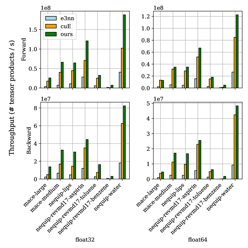
Figure 5: Throughput of CG tensor products (batch size 50K), kernel B configurations without SpMM kernel fusion. On difficult configurations like Nequip-benzene with massive output vector lengths, we exhibit up to 10x improvement over e3nn and cuE.

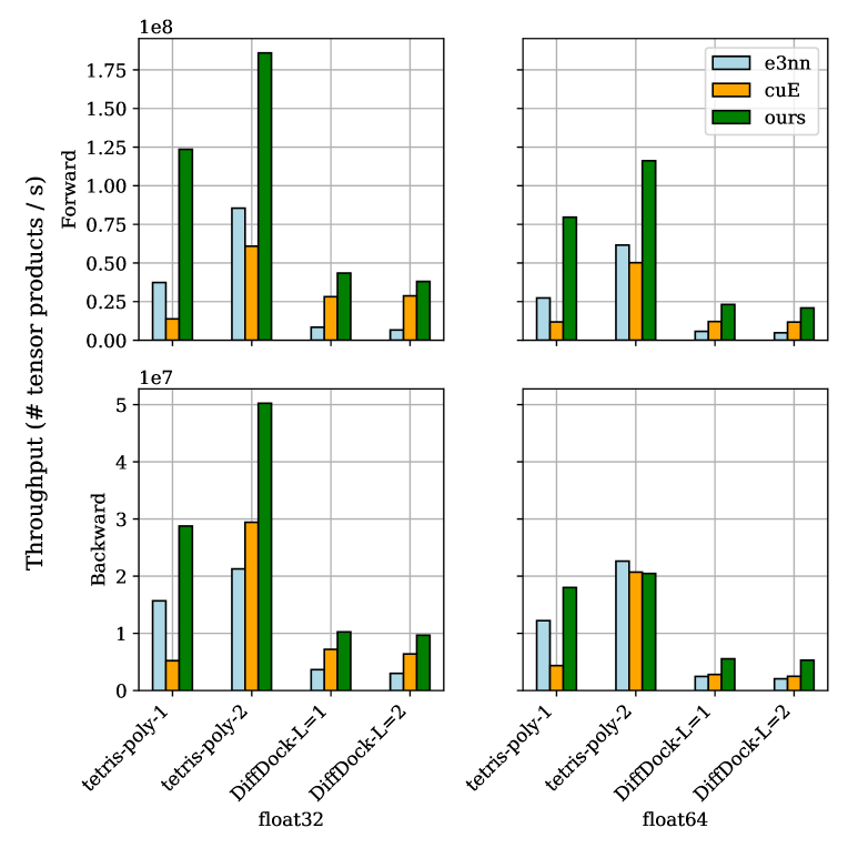
Figure 6: Throughput of CG tensor products (batch size 50k), kernel C configurations. We exhibit up to 2x speedup over cuE on the DiffDock tensor products.

We first profiled our kernels on a large collection of model configurations used by Nequip [4] and MACE [2]. For each model, we selected the most expensive tensor product to benchmark.

Figure 5 shows the results of our profiling on configurations that use only Kernel B (see Figure 3). Our median FP32 speedup over e3nn was 5.7x, resp. 5.0x, for the forward and backward passes, with a maximum of 9.3x for the forward pass. We observed a median speedup of 1.7x over cuE for the FP32 forward pass, which drops to 1.2x in FP64 precision. We achieve parity with cuE on the larger MACE model in FP64 precision; here, both cuE and our kernels have nearly identical runtime. We explore this configuration further in our kernel fusion benchmarks. Our implementation exhibits an outsized speedup (10-20x) on the Nequip-benzene configuration over both baselines. Here, the large output vector size ($\sim 20\textrm{k}$ data words) requires careful shared memory management, which our scheduling algorithm provides.

To benchmark kernel C, we used the Tetris polynomial from e3nn’s documentation [9] and two configurations based on DiffDock [6]. We exhibit between 1.4x and 2.1x speedup over cuE for both forward and backward passes on DiffDock. The Tetris polynomial uses an identical weight matrix $\bm{W}$ for all inputs $\bm{x}_{1}...\bm{x}_{B}$ and $\bm{y}_{1}...\bm{y}_{B}$, a feature unique to this model. We use atomic accumulation in the backward pass to compute the gradient with respect to the shared weights, which reduces our relative speedup in FP64 precision. Our speedups over all configurations are less dramatic for kernel C, which has a workload dominated by the small dense matrix multiplication in Algorithms 2 and 3.

4.2 Roofline Analysis

ID	Description	Dir.	AI	TFLOP/s
				cuE	ours
1	128x1e$\ \times\$1x1e $\rightarrow$ 128x1e (B)	F	0.7	0.27	1.12
		B	1.2	0.43	1.84
2	128x2e$\ \times\$1x1e $\rightarrow$ 128x2e (B)	F	1.2	0.58	1.82
		B	2.1	0.73	3.22
3	128x3e$\ \times\$1x3e $\rightarrow$ 128x3e (B)	F	2.2	1.22	3.50
		B	4.1	1.19	6.22
4	128x5e$\ \times\$1x5e $\rightarrow$ 128x3e (B)	F	4.1	1.69	6.35
		B	7.4	1.39	9.77
5	128x5e$\ \times\$1x3e $\rightarrow$ 128x5e (B)	F	3.4	1.70	5.24
		B	6.5	1.35	8.94
6	128x6e$\ \times\$1x3e $\rightarrow$ 128x6e (B)	F	3.6	1.82	5.61
		B	6.9	1.41	9.24
7	128x7e$\ \times\$1x4e $\rightarrow$ 128x7e (B)	F	4.9	2.07	7.65
		B	9.5	1.46	10.67
8	128x7e$\ \times\$1x7e $\rightarrow$ 128x7e (B)	F	6.3	2.21	9.71
		B	12.3	1.56	11.30

Table 2: Arithmetic intensity (AI) and throughput for our kernels vs. cuEquivariance (cuE) for varied problem configurations, FP32 forward and backward passes.

We conducted a roofline analysis [35] by profiling our forward / backward pass implementations on varied input configurations. We profiled tensor products with a single “B” subkernel (see Figure 3) with FP32 precision, core building blocks for models like Nequip and MACE. The arithmetic intensity of the CG tensor product depends on the structure of the sparse tensor, and we profiled configurations with progressively increasing arithmetic intensity.

Figure 7 and Table 2 show our profiling results, which indicate consistently high compute and bandwidth utilization for our kernels. In the bandwidth-limited portion of the diagram, our implementation increases its throughput linearly to match increasing arithmetic intensity in the input configurations. By contrast, the throughput of cuEquivariance’s forward pass stagnates. Our kernel performance saturates at 58% of the FP32 peak, possibly because Algorithms 2 and 3 contain contain a significant fraction of non fused-multiply-add (FMA) instructions.

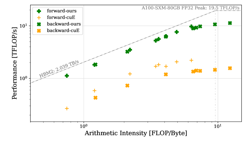
Figure 7: Roofline analysis of our kernels on the input configurations from Table 2, batch size 200k. Our kernel performance closely tracks the slope of the global memory roofline, whereas cuE plateaus early in the memory-bandwidth limited region of the plot.

4.3 Kernel Fusion Benchmarks

We conducted our kernel fusion experiments on three molecular structure graphs listed in Table 3. We downloaded the atomic structures of human dihydrofolate deductase (DHFR) and the SARS-COV-2 glycoprotein spike from the Protein Data Bank and constructed a radius-neighbors graph for each using Scikit-Learn [27]. The carbon lattice was provided to us as a representative workload for MACE [3].

Graph	Nodes	Adj. Matrix NNZ
DHFR 1DRF	1.8K	56K
COVID spike 6VXX	23K	136K
Carbon lattice	1K	158K

Table 3: Molecular graphs for kernel fusion experiments.

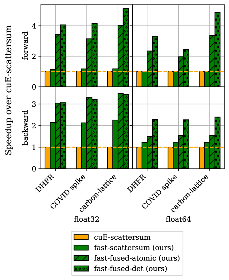
Figure 8: Speedup of our fused MACE convolution kernels over cuE-scattersum, which calls cuEquivariance and follows it by a scatter-sum operation.

Figure 8 shows the speedup of our fused implementations benchmarked on the most expensive tensor product in the MACE-large model. Our baseline, “cuE-scattersum”, implements the unfused strategy in Section 3.5 by duplicating node embeddings, executing a large batch of tensor products with cuEquivariance, and finally performing row-based reduction by keys. The “fast-scattersum” implementation adopts the same method with our kernels instead of our cuEquivariance. Without kernel fusion, our implementation and cuEquivariance exhibit nearly identical performance across all configurations except the backwards pass in FP32 precision (we are 2x faster). The performance gap is smaller than in Figure 5 since the scatter-sum accounts for 50-60% of the runtime.

The“fast-fused-det” and “fast-fused-atomic” implementations use the memory-efficient formulations from Section 3.5, offering dramatically faster performance as a result. Our deterministic fused algorithm offers up to 4.8x speedup over cuEquivariance for the forward pass and 3.5x on the backward pass. Our poorest performance occurs with the atomic algorithm in FP64 precision for the backward pass, where we still see 1.3x-1.4x speedup over cuEquivariance.

4.4 Acceleration of MACE

The MACE foundation model [3], trained on data from the Materials Project [12], implements the equivariant graph neural network architecture depicted in Figure 4B. We patched MACE to sort nonzeros of its atomic adjacency matrix according to compressed sparse row (CSR) order, as well as compute the transpose permutation. We then substituted Algorithm 4 in place of the existing graph convolution to measure performance relative to other kernel providers. Our benchmark was conducted on the carbon lattice listed in Table 3.

Figure 9 (left) compares the rate of molecular dynamics simulation among the different kernel providers. We benchmarked cuE with the optimal data layout for its irreps and included optimizations for symmetric tensor contraction, linear combination layers, and graph convolution. In FP32 precision, we provide 5.3x speeedup over e3nn and 1.5x over cuEquivariance. In FP64 precision, we offer 6.6x speedup over e3nn and 1.43x over cuEquivariance. Because we do not materialize the intermediate tensor product outputs for each edge, our fused kernels reduce the model memory footprint by roughly 158x.

Figure 9 (right) breaks down the device runtime spent in various kernels traced by the PyTorch profiler. The sum of kernel runtimes in the right figure differs from the times measured in the left figure due to device idle time. Notice that our speedup comes entirely from accelerating the equivariant graph convolution; the CTP kernel and scatter-sum runtime is 4x faster in our implementation compared to cuE in FP32 precision.

By contrast, cuEquivariance also accelerates a “symmetric contraction” kernel specific to MACE (reducing the runtime counted in “Other” category), and we leave these kernels to future work. Our runtime in the “Other” category can be reduced through torch.compile(), but we did not include this optimization in fairness to cuE (errors in compilation) and e3nn (memory constraints). We plan to update these benchmarks when further support is added in cuE.

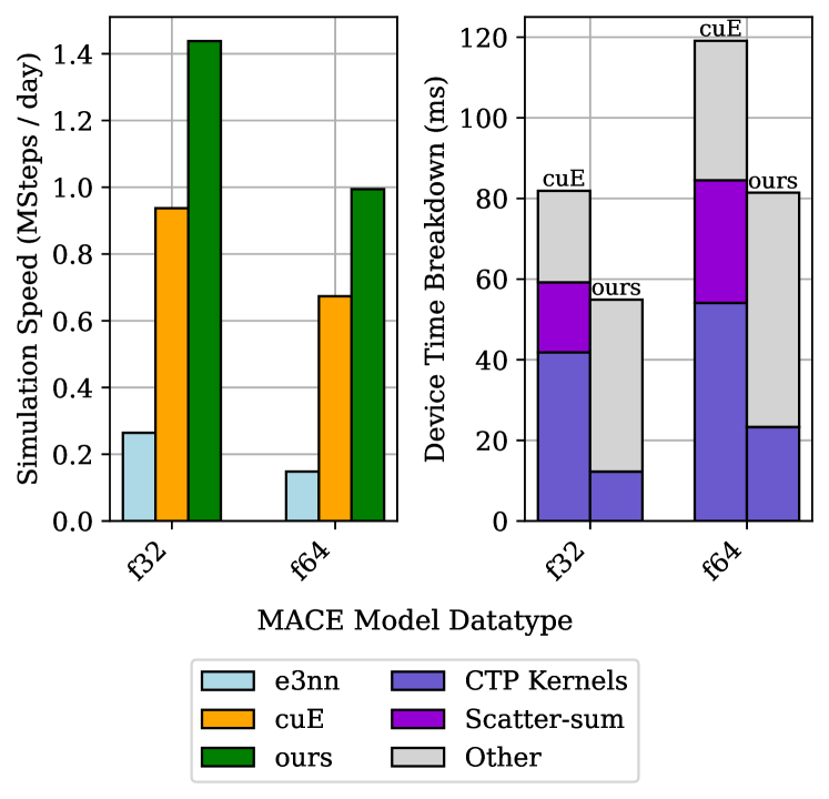
Figure 9: Simulation speed of MACE for varying kernel provider and device time breakdown (no torch.compile()).

5 Conclusions and Further Work

We have established that our sparse kernels achieve consistently high performance on the most common primitives used in equivariant deep neural networks. Our speedup over e3nn and cuEquivariance prove that a sparsity-aware, JIT-compiled kernel can outperform strategies based entirely on dense linear algebra. We see several avenues for future progress:

• Low Precision Data and MMA Support: Our kernels rely on the single-instruction multiple thread (SIMT) cores for FP32 and FP64 floating point arithmetic. Modern GPUs offer specialized hardware for lower-precision calculation, both using SIMT cores and within matrix-multiply-accumulate (MMA) units. We plan to harness these capabilities in the future.

• Accelerator and language support: In contrast to cuEquivariance, all of our code is open-source. We hope to cross compile our kernels to HIP for AMD GPUs, as well as offer bindings for JAX and the Julia scientific computing language.

• Integration into new models: Our software remains accessible to newcomers while delivering the high performance required for massive inference workloads. In conjunction with domain experts, we hope to apply our library to train larger, more expressive equivariant deep neural networks.

References

- Anderson et al. [2019] Brandon Anderson, Truong-Son Hy, and Risi Kondor. Cormorant: covariant molecular neural networks. In Proceedings of the 33rd International Conference on Neural Information Processing Systems, Red Hook, NY, USA, 2019. Curran Associates Inc.
- Batatia et al. [2022] Ilyes Batatia, David Peter Kovacs, Gregor N. C. Simm, Christoph Ortner, and Gabor Csanyi. MACE: Higher order equivariant message passing neural networks for fast and accurate force fields. In Alice H. Oh, Alekh Agarwal, Danielle Belgrave, and Kyunghyun Cho, editors, Advances in Neural Information Processing Systems, 2022. URL https://openreview.net/forum?id=YPpSngE-ZU.
- Batatia et al. [2024] Ilyes Batatia, Philipp Benner, Yuan Chiang, Alin M. Elena, Dávid P. Kovács, Janosh Riebesell, Xavier R. Advincula, Mark Asta, Matthew Avaylon, William J. Baldwin, Fabian Berger, Noam Bernstein, Arghya Bhowmik, Samuel M. Blau, Vlad Cărare, James P. Darby, Sandip De, Flaviano Della Pia, Volker L. Deringer, Rokas Elijošius, Zakariya El-Machachi, Fabio Falcioni, Edvin Fako, Andrea C. Ferrari, Annalena Genreith-Schriever, Janine George, Rhys E. A. Goodall, Clare P. Grey, Petr Grigorev, Shuang Han, Will Handley, Hendrik H. Heenen, Kersti Hermansson, Christian Holm, Jad Jaafar, Stephan Hofmann, Konstantin S. Jakob, Hyunwook Jung, Venkat Kapil, Aaron D. Kaplan, Nima Karimitari, James R. Kermode, Namu Kroupa, Jolla Kullgren, Matthew C. Kuner, Domantas Kuryla, Guoda Liepuoniute, Johannes T. Margraf, Ioan-Bogdan Magdău, Angelos Michaelides, J. Harry Moore, Aakash A. Naik, Samuel P. Niblett, Sam Walton Norwood, Niamh O’Neill, Christoph Ortner, Kristin A. Persson, Karsten Reuter, Andrew S. Rosen, Lars L. Schaaf, Christoph Schran, Benjamin X. Shi, Eric Sivonxay, Tamás K. Stenczel, Viktor Svahn, Christopher Sutton, Thomas D. Swinburne, Jules Tilly, Cas van der Oord, Eszter Varga-Umbrich, Tejs Vegge, Martin Vondrák, Yangshuai Wang, William C. Witt, Fabian Zills, and Gábor Csányi. A foundation model for atomistic materials chemistry, 2024. URL https://arxiv.org/abs/2401.00096.
- Batzner et al. [2022] Simon Batzner, Albert Musaelian, Lixin Sun, Mario Geiger, Jonathan P. Mailoa, Mordechai Kornbluth, Nicola Molinari, Tess E. Smidt, and Boris Kozinsky. E(3)-equivariant graph neural networks for data-efficient and accurate interatomic potentials. Nature Communications, 13(1):2453, May 2022. ISSN 2041-1723. doi: 10.1038/s41467-022-29939-5. URL https://doi.org/10.1038/s41467-022-29939-5.
- Corporation [2020] NVIDIA Corporation. NVIDIA A100 tensor core gpu architecture. Technical report, NVIDIA, 2020. URL https://images.nvidia.com/aem-dam/en-zz/Solutions/data-center/nvidia-ampere-architecture-whitepaper.pdf.
- Corso et al. [2023] Gabriele Corso, Hannes Stärk, Bowen Jing, Regina Barzilay, and Tommi S. Jaakkola. Diffdock: Diffusion steps, twists, and turns for molecular docking. In The Eleventh International Conference on Learning Representations, 2023.
- Fuchs et al. [2020] Fabian Fuchs, Daniel Worrall, Volker Fischer, and Max Welling. SE(3)-transformers: 3d roto-translation equivariant attention networks. In H. Larochelle, M. Ranzato, R. Hadsell, M.F. Balcan, and H. Lin, editors, Advances in Neural Information Processing Systems, volume 33, pages 1970–1981. Curran Associates, Inc., 2020. URL https://proceedings.neurips.cc/paper_files/paper/2020/file/15231a7ce4ba789d13b722cc5c955834-Paper.pdf.
- Geiger and Smidt [2022] Mario Geiger and Tess Smidt. e3nn: Euclidean neural networks, 2022. URL https://arxiv.org/abs/2207.09453.
- Geiger et al. [2022] Mario Geiger, Tess Smidt, Alby M., Benjamin Kurt Miller, Wouter Boomsma, Bradley Dice, Kostiantyn Lapchevskyi, Maurice Weiler, Michał Tyszkiewicz, Simon Batzner, Dylan Madisetti, Martin Uhrin, Jes Frellsen, Nuri Jung, Sophia Sanborn, Mingjian Wen, Josh Rackers, Marcel Rød, and Michael Bailey. Euclidean neural networks: e3nn, April 2022. URL https://github.com/e3nn/e3nn/releases/tag/0.5.0.
- Geiger et al. [2024] Mario Geiger, Emine Kucukbenli, Becca Zandstein, and Kyle Tretina. Accelerate drug and material discovery with new math library NVIDIA cuEquivariance, 11 2024. URL https://developer.nvidia.com/blog/accelerate-drug-and-material-discovery-with-new-math-library-nvidia-cuequivariance/.
- Helal et al. [2021] Ahmed E. Helal, Jan Laukemann, Fabio Checconi, Jesmin Jahan Tithi, Teresa Ranadive, Fabrizio Petrini, and Jeewhan Choi. Alto: adaptive linearized storage of sparse tensors. In Proceedings of the 35th ACM International Conference on Supercomputing, ICS ’21, page 404–416, New York, NY, USA, 2021. Association for Computing Machinery. ISBN 9781450383356. doi: 10.1145/3447818.3461703. URL https://doi.org/10.1145/3447818.3461703.
- Jain et al. [2013] Anubhav Jain, Shyue Ping Ong, Geoffroy Hautier, Wei Chen, William Davidson Richards, Stephen Dacek, Shreyas Cholia, Dan Gunter, David Skinner, Gerbrand Ceder, and Kristin A. Persson. Commentary: The materials project: A materials genome approach to accelerating materials innovation. APL Materials, 1(1):011002, 07 2013. ISSN 2166-532X. doi: 10.1063/1.4812323. URL https://doi.org/10.1063/1.4812323.
- Johansson et al. [2013] J.R. Johansson, P.D. Nation, and F. Nori. QuTiP 2: A Python framework for the dynamics of open quantum systems. Computer Physics Communications, 184(4):1234–1240, apr 2013. doi: 10.1016/j.cpc.2012.11.019. URL https://doi.org/10.1016/j.cpc.2012.11.019.
- Jumper et al. [2021] John Jumper, Richard Evans, Alexander Pritzel, Tim Green, Michael Figurnov, Olaf Ronneberger, Kathryn Tunyasuvunakool, Russ Bates, Augustin Žídek, Anna Potapenko, Alex Bridgland, Clemens Meyer, Simon A. A. Kohl, Andrew J. Ballard, Andrew Cowie, Bernardino Romera-Paredes, Stanislav Nikolov, Rishub Jain, Jonas Adler, Trevor Back, Stig Petersen, David Reiman, Ellen Clancy, Michal Zielinski, Martin Steinegger, Michalina Pacholska, Tamas Berghammer, Sebastian Bodenstein, David Silver, Oriol Vinyals, Andrew W. Senior, Koray Kavukcuoglu, Pushmeet Kohli, and Demis Hassabis. Highly accurate protein structure prediction with AlphaFold. Nature, 596(7873):583–589, Aug 2021. ISSN 1476-4687. doi: 10.1038/s41586-021-03819-2.
- Karniadakis et al. [2021] George Em Karniadakis, Ioannis G. Kevrekidis, Lu Lu, Paris Perdikaris, Sifan Wang, and Liu Yang. Physics-informed machine learning. Nature Reviews Physics, 3(6):422–440, Jun 2021. ISSN 2522-5820. doi: 10.1038/s42254-021-00314-5.
- Koker [2024] Teddy Koker. e3nn.c, November 2024. URL https://github.com/teddykoker/e3nn.c.
- Koker et al. [2024] Teddy Koker, Keegan Quigley, Eric Taw, Kevin Tibbetts, and Lin Li. Higher-order equivariant neural networks for charge density prediction in materials. npj Computational Materials, 10(1):161, Jul 2024. ISSN 2057-3960. doi: 10.1038/s41524-024-01343-1.
- Kondor and Thiede [2024] Risi Kondor and Erik Henning Thiede. Gelib, 07 2024. URL https://github.com/risi-kondor/GElib.
- Kondor et al. [2018] Risi Kondor, Zhen Lin, and Shubhendu Trivedi. Clebsch–Gordan nets: a fully Fourier space spherical convolutional neural network. In Proceedings of the 32nd International Conference on Neural Information Processing Systems, NIPS’18, page 10138–10147, Red Hook, NY, USA, 2018. Curran Associates Inc.
- Lambert et al. [2024] Neill Lambert, Eric Giguère, Paul Menczel, Boxi Li, Patrick Hopf, Gerardo Suárez, Marc Gali, Jake Lishman, Rushiraj Gadhvi, Rochisha Agarwal, Asier Galicia, Nathan Shammah, Paul D. Nation, J. R. Johansson, Shahnawaz Ahmed, Simon Cross, Alexander Pitchford, and Franco Nori. QuTiP 5: The quantum toolbox in Python, 2024. URL https://arxiv.org/abs/2412.04705.
- Lee et al. [2024a] Kin Long Kelvin Lee, Mikhail Galkin, and Santiago Miret. Deconstructing equivariant representations in molecular systems. In AI for Accelerated Materials Design - NeurIPS 2024, 2024a. URL https://openreview.net/forum?id=pshyLoyzRn.
- Lee et al. [2024b] Kin Long Kelvin Lee, Mikhail Galkin, and Santiago Miret. Scaling computational performance of spherical harmonics kernels with Triton. In AI for Accelerated Materials Design - Vienna 2024, 2024b. URL https://openreview.net/forum?id=ftK00FO5wq.
- Liao and Smidt [2023] Yi-Lun Liao and Tess Smidt. Equiformer: Equivariant graph attention transformer for 3D atomistic graphs. In International Conference on Learning Representations, 2023. URL https://openreview.net/forum?id=KwmPfARgOTD.
- Lim and Nelson [2023] Lek-Heng Lim and Bradley J Nelson. What is… an equivariant neural network? Notices of the American Mathematical Society, 70(4):619–624, 4 2023. ISSN 0002-9920, 1088-9477. doi: 10.1090/noti2666. URL https://www.ams.org/notices/202304/rnoti-p619.pdf.
- Luo et al. [2024] Shengjie Luo, Tianlang Chen, and Aditi S. Krishnapriyan. Enabling efficient equivariant operations in the Fourier basis via gaunt tensor products. In The Twelfth International Conference on Learning Representations, 2024. URL https://openreview.net/forum?id=mhyQXJ6JsK.
- Musaelian et al. [2023] Albert Musaelian, Simon Batzner, Anders Johansson, Lixin Sun, Cameron J. Owen, Mordechai Kornbluth, and Boris Kozinsky. Learning local equivariant representations for large-scale atomistic dynamics. Nature Communications, 14(1):579, Feb 2023. ISSN 2041-1723. doi: 10.1038/s41467-023-36329-y.
- Pedregosa et al. [2011] F. Pedregosa, G. Varoquaux, A. Gramfort, V. Michel, B. Thirion, O. Grisel, M. Blondel, P. Prettenhofer, R. Weiss, V. Dubourg, J. Vanderplas, A. Passos, D. Cournapeau, M. Brucher, M. Perrot, and E. Duchesnay. Scikit-learn: Machine learning in Python. Journal of Machine Learning Research, 12:2825–2830, 2011.
- Qu and Krishnapriyan [2024] Eric Qu and Aditi S. Krishnapriyan. The importance of being scalable: Improving the speed and accuracy of neural network interatomic potentials across chemical domains, 10 2024. URL http://arxiv.org/abs/2410.24169.
- Schütt et al. [2021] Kristof Schütt, Oliver Unke, and Michael Gastegger. Equivariant message passing for the prediction of tensorial properties and molecular spectra. In Marina Meila and Tong Zhang, editors, Proceedings of the 38th International Conference on Machine Learning, volume 139 of Proceedings of Machine Learning Research, pages 9377–9388. PMLR, 18–24 Jul 2021.
- Smith and Karypis [2015] Shaden Smith and George Karypis. Tensor-matrix products with a compressed sparse tensor. In Proceedings of the 5th Workshop on Irregular Applications: Architectures and Algorithms, IA¡sup¿3¡/sup¿ ’15, New York, NY, USA, 2015. Association for Computing Machinery. ISBN 9781450340014. doi: 10.1145/2833179.2833183.
- Thakkar et al. [2023] Vijay Thakkar, Pradeep Ramani, Cris Cecka, Aniket Shivam, Honghao Lu, Ethan Yan, Jack Kosaian, Mark Hoemmen, Haicheng Wu, Andrew Kerr, Matt Nicely, Duane Merrill, Dustyn Blasig, Fengqi Qiao, Piotr Majcher, Paul Springer, Markus Hohnerbach, Jin Wang, and Manish Gupta. CUTLASS, January 2023. URL https://github.com/NVIDIA/cutlass.
- Thomas et al. [2018] Nathaniel Thomas, Tess Smidt, Steven Kearnes, Lusann Yang, Li Li, Kai Kohlhoff, and Patrick Riley. Tensor field networks: Rotation- and translation-equivariant neural networks for 3D point clouds, 2018.
- Unke and Maennel [2024] Oliver T. Unke and Hartmut Maennel. E3x: -equivariant deep learning made easy, 2024. URL https://arxiv.org/abs/2401.07595.
- Weiler et al. [2018] Maurice Weiler, Mario Geiger, Max Welling, Wouter Boomsma, and Taco Cohen. 3D steerable cnns: learning rotationally equivariant features in volumetric data. In Proceedings of the 32nd International Conference on Neural Information Processing Systems, NIPS’18, page 10402–10413, Red Hook, NY, USA, 2018. Curran Associates Inc.
- Williams et al. [2009] Samuel Williams, Andrew Waterman, and David Patterson. Roofline: an insightful visual performance model for multicore architectures. Commun. ACM, 52(4):65–76, April 2009. ISSN 0001-0782. doi: 10.1145/1498765.1498785. URL https://doi.org/10.1145/1498765.1498785.
- Xie et al. [2024] YuQing Xie, Ameya Daigavane, Mit Kotak, and Tess Smidt. The price of freedom: Exploring tradeoffs between expressivity and computational efficiency in equivariant tensor products. In ICML 2024 Workshop on Geometry-grounded Representation Learning and Generative Modeling, 6 2024. URL https://openreview.net/forum?id=0HHidbjwcf.
- Yang et al. [2018] Carl Yang, Aydın Buluç, and John D. Owens. Design principles for sparse matrix multiplication on the gpu. In Euro-Par 2018: Parallel Processing: 24th International Conference on Parallel and Distributed Computing, Turin, Italy, August 27 - 31, 2018, Proceedings, page 672–687, Berlin, Heidelberg, 2018. Springer-Verlag. ISBN 978-3-319-96982-4. doi: 10.1007/978-3-319-96983-1˙48.