GS-LiDAR: Generating Realistic LiDAR Point Clouds with Panoramic Gaussian Splatting

Abstract

LiDAR novel view synthesis (NVS) has emerged as a novel task within LiDAR simulation, offering valuable simulated point cloud data from novel viewpoints to aid in autonomous driving systems. However, existing LiDAR NVS methods typically rely on neural radiance fields (NeRF) as their 3D representation, which incurs significant computational costs in both training and rendering. Moreover, NeRF and its variants are designed for symmetrical scenes, making them ill-suited for driving scenarios. To address these challenges, we propose GS-LiDAR, a novel framework for generating realistic LiDAR point clouds with panoramic Gaussian splatting. Our approach employs 2D Gaussian primitives with periodic vibration properties, allowing for precise geometric reconstruction of both static and dynamic elements in driving scenarios. We further introduce a novel panoramic rendering technique with explicit ray-splat intersection, guided by panoramic LiDAR supervision. By incorporating intensity and ray-drop spherical harmonic (SH) coefficients into the Gaussian primitives, we enhance the realism of the rendered point clouds. Extensive experiments on KITTI-360 and nuScenes demonstrate the superiority of our method in terms of quantitative metrics, visual quality, as well as training and rendering efficiency.

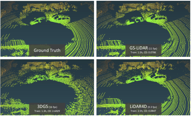
Figure 1: GS-LiDAR achieves superior LiDAR simulation quality for novel view synthesis while maintaining fast training and rendering speed. For more results on static scene, dynamic scene, lane shifting and novel trajectory, please refer to the video in our supplementary material.

1 Introduction

Captured data in driving scenarios is critically important, as it serves to train and simulate autonomous driving systems. However, the collection of driving data is both costly and inefficient. This underscores the necessity for a LiDAR simulation algorithm capable of generating realistic LiDAR data more efficiently. A common approach in the field is to reconstruct 3D street scenes from sparse data, which can then be used to generate novel view data. Most previous works (Xie et al., 2023b; Yang et al., 2024a; Chen et al., 2023a; Yan et al., 2024) have concentrated on novel view synthesis for cameras. These approaches use RGB images captured by vehicle-mounted cameras as input to reconstruct 3D scenes and render images from novel perspectives. Although significant progress has been made in camera-based novel view synthesis, the simulation of LiDAR remains underexplored. Due to the inherent sparsity of LiDAR point clouds, the challenge lies in accurately reconstructing 3D scenes using only LiDAR data. Furthermore, LiDAR sensors do not capture all emitted beams, as factors such as the reflective properties of objects affect beam reception, leading to point cloud dropout, which further increases the difficulty of 3D scene reconstruction.

Traditional LiDAR simulation methods can be broadly classified into two categories: virtual environment modeling (Dosovitskiy et al., 2017; Shah et al., 2018; Koenig & Howard, 2004) and reconstruction-based approaches (Manivasagam et al., 2020; Li et al., 2023; Guillard et al., 2022). The former involves creating 3D virtual worlds using physics engines and handcrafted 3D assets, though these simulators are constrained by the limited diversity and high cost of generating 3D assets. Additionally, there remains a significant domain gap between simulations and the real world. In contrast, reconstruction-based methods aim to address these limitations by reconstructing 3D assets from real-world captured data. However, the complexity of multi-step algorithms in this category limits their practical application in industry.

In recent years, neural radiance field (NeRF) (Mildenhall et al., 2020) has emerged as a foundational technique in the field of 3D reconstruction. With its effective implicit representation and high-quality volumetric rendering, NeRF has been proposed as a novel approach for LiDAR simulation. NeRF-LiDAR (Zhang et al., 2024) utilizes real images and LiDAR data to learn a Neural Radiance Field, generating point clouds and rendering semantic labels. On the other hand, LiDAR-NeRF (Tao et al., 2023) introduces a novel LiDAR view synthesis task, which uses only LiDAR data as input to reconstruct a 3D scene. However, LiDAR-NeRF is limited to modeling static scenes, whereas dynamic vehicles and pedestrians are common in driving scenarios. To address this, LiDAR4D (Zheng et al., 2024) introduces a hybrid 4D representation for novel space-time LiDAR view synthesis. Although these NeRF-based methods mark significant progress compared to traditional techniques, they suffer from slow training and rendering speeds, a limitation inherent to NeRF. Furthermore, efficient NeRF-based architectures like HashGrid (Müller et al., 2022), designed for symmetrical scenes, are not well-suited for driving scenarios.

In this paper, we propose GS-LiDAR, a novel framework for generating realistic LiDAR point clouds using panoramic Gaussian splatting. While 3D Gaussian splatting struggles with geometric modeling and tends to overfit sparse views, we leverage view-consistent 2D Gaussian primitives Huang et al. (2024) for more accurate geometric representation. Moreover, considering the dynamic nature of driving scenarios, we introduce periodic vibration properties Chen et al. (2023a) into the Gaussian primitives, enabling the uniform representation of various objects and elements in dynamic environments. Focusing on the task of novel LiDAR view synthesis, we introduce a novel panoramic rendering process to facilitate fast and efficient rendering of panoramic depth maps using 2D Gaussian primitives. Through carefully designed ray-splat intersections, the resulting panoramic depth maps are geometrically accurate and view-consistent. Each Gaussian is assigned additional LiDAR-specific attributes, such as view-dependent intensity and ray-drop probability, which are aggregated into intensity maps and ray-drop maps through alpha-blending in the splatting process. By using ground-truth LiDAR range maps and intensity maps for supervision, GS-LiDAR can effectively simulate LiDAR point clouds. As illustrated in Figure 1, GS-LiDAR achieves superior LiDAR simulation quality in novel LiDAR view synthesis and significantly outperforms the previous state-of-the-art method, LiDAR4D (Zheng et al., 2024), in both training and rendering speed.

We conduct extensive experiments to evaluate the effectiveness of our method on two major benchmarks: KITTI-360 (Liao et al., 2022) and nuScenes (Caesar et al., 2020). For static scenes, we test our approach on the KITTI-360 dataset, achieving a substantial 10.7% reduction in the RMSE metric compared to the leading competitor, LiDAR4D (Zheng et al., 2024). For dynamic scenes, our method outperforms LiDAR4D, with RMSE reductions of 11.5% on KITTI-360 and 13.1% on nuScenes. Moreover, our approach demonstrated significantly faster training and rendering times than previous NeRF-based methods, with a speedup of 1.67 times in training and a notable increase of 31 times in rendering LiDAR novel views compared to LiDAR4D.

Our contributions are summarized as follows: (1) We propose GS-LiDAR, a novel differentiable framework for generating realistic LiDAR point clouds. (2) We employ 2D Gaussian primitives with periodic vibration properties, enabling precise geometric reconstruction of various objects and elements in dynamic scenarios. (3) We introduce a novel panoramic rendering technique based on 2D Gaussian primitives, with geometrically accurate ray-splat intersection, where the rendered panoramic maps are supervised by the ground-truth data. (4) Extensive experiments demonstrate the superiority of our method across quantitative metrics, visual quality, as well as training and rendering speeds, when compared to previous approaches.

2 Related work

Novel view synthesis

Novel view synthesis (NVS) is a critical and challenging aspect of 3D reconstruction. Since the advent of neural radiance fields (NeRF) (Mildenhall et al., 2020), there have been significant advancements in 3D reconstruction and NVS. NeRF utilizes a multi-layer perceptron (MLP) to model geometric shapes and view-dependent appearances, rendering through volume rendering. NeRF has demonstrated that implicit radiance fields can effectively learn scene representations and synthesize high-quality novel views. Despite its profound impact, NeRF faces notable challenges, including slow rendering speeds and aliasing. To address these issues, various research efforts (Barron et al., 2021; 2022; 2023; Hu et al., 2023; Reiser et al., 2021; Yu et al., 2021; Reiser et al., 2023; Hedman et al., 2021; Yariv et al., 2023; Chen et al., 2023c; 2022; Müller et al., 2022; Liu et al., 2020; Sun et al., 2022; Chen et al., 2023b; Fridovich-Keil et al., 2022) have developed variants that focus on enhancing rendering quality as well as accelerating training and rendering speeds. Recently, 3D Gaussian splatting (3DGS) (Kerbl et al., 2023) has introduced a point-based 3D scene representation that innovatively combines high-quality alpha-blending with rapid rasterization. 3DGS has been swiftly extended to various domains to enhance its rendering capabilities (Xie et al., 2023a; Huang et al., 2024; Gao et al., 2024) and its potential to represent dynamic scenes (Yang et al., 2024b; Yan et al., 2024; Zielonka et al., 2023; Chen et al., 2023a). In this paper, we adopt 2D Gaussian primitives with periodic vibration properties as scene representation to characterize the accurate geometry of both static and dynamic elements.

LiDAR simulation

Traditional simulators can be classified into two categories. The first type of method (Dosovitskiy et al., 2017; Shah et al., 2018; Koenig & Howard, 2004) utilizes physics engines to generate LiDAR point clouds through ray casting within handcrafted virtual environments. However, these simulators are limited by their diversity and the high cost of 3D assets, and they exhibit a significant domain gap when compared to real-world data. In contrast, the second type of methods (Manivasagam et al., 2020; Li et al., 2023; Guillard et al., 2022) have sought to address these limitations by reconstructing scenes from real data for simulation. For instance, LiDARsim (Manivasagam et al., 2020) and PCGen (Li et al., 2023) utilize a multi-step, data-driven approach to simulate point clouds from real data. However, the complexity of these multiple steps impacts their applicability and scalability. More recent works (Tao et al., 2023; Zhang et al., 2024; Zheng et al., 2024; Xue et al., 2024; Tao et al., 2024; Wu et al., 2024) have utilized NeRF for scene reconstruction and LiDAR simulation, achieving higher quality and more reliable results. However, NeRF is time-consuming due to its implicit representation and exhaustive ray marching. Moreover, NeRF and its variants are mostly designed for symmetrical scenes, making them ill-suited to the driving scenarios. To this end, GS-LiDAR employs the explicit representation of Gaussian splatting, which enables efficient and flexible LiDAR simulation.

3 Method

In this section, we propose GS-LiDAR, a novel framework for generating realistic LiDAR point clouds with Gaussian splatting. We begin by introducing the necessary background on 3D Gaussian splatting in Section 3.1. For geometrically accurate reconstruction and the modeling of both static and dynamic elements, we employ 2D Gaussian primitives with periodic vibration properties as our scene representation, as outlined in Section 3.2. To integrate LiDAR supervision, we propose an innovative panoramic rendering technique with explicit ray-splat intersection, described in Section 3.3. Next, we detail the LiDAR modeling approach, including the rendering of depth maps, intensity maps, and ray-drop probability maps, in Section 3.4. Finally, in Section 3.5, we discuss the various functions used to optimize the scenes. An overview of our pipeline is provided in Figure 2.

3.1 Preliminary: 3D Gaussian splatting

3D Gaussian splatting (3DGS) (Kerbl et al., 2023) employs a set of anisotropic Gaussian primitives to represent a static 3D scene, which is subsequently rendered vis differentiable splatting. By utilizing a tile-based rasterizer, this approach facilitates the real-time rendering of novel views with high visual fidelity. Each Gaussian primitive is characterized by a position vector ${\bm{\mu}}\in\mathbb{R}^{3}$, a covariance matrix ${\bm{\Sigma}}\in\mathbb{R}^{3\times 3}$, an opacity parameter $o\in(0,1)$, and color $\bm{c}\in\mathbb{R}^{3}$ modeled by spherical harmonics (SH). The influence $\mathcal{G}({\bm{x}})$ of a given Gaussian primitive on a spatial position ${\bm{x}}$ is defined by an unnormalized Gaussian function:

$$\mathcal{G}({\bm{x}})=\exp({-\frac{1}{2}({\bm{x}}-{\bm{\mu}})^{\top}{\bm{\Sigma}}^{-1}({\bm{x}}-{\bm{\mu}})}).$$ (1)

To render an image, the 3D Gaussian primitives are initially transformed into the camera coordinate system via the view transformation matrix ${\bm{W}}$. Following this transformation, each Gaussian primitive is projected onto the image plane through a local affine transformation ${\bm{J}}$, which maps the 3D structure into 2D image space. The 2D covariance matrix ${\bm{\Sigma}}^{\prime}$ of the projected Gaussian primitive in camera coordinates is computed as: ${\bm{\Sigma}}^{\prime}={\bm{J}}{\bm{W}}{\bm{\Sigma}}{\bm{W}}^{\top}{\bm{J}}^{\top}$. The final rendering process employs alpha-blending, wherein the color ${\bm{c}}$ of a target pixel is obtained by aggregating the contribution $\mathcal{G}^{\prime}$ of each relevant projected 2D Gaussian, proceeding from front to back:

$${\bm{c}}=\sum^{K}_{k=1}{\bm{c}}_{k}\,o_{k}\,\mathcal{G}^{\prime}_{k}\prod_{j=1}^{k-1}(1-o_{j}\,\mathcal{G}^{\prime}_{j}),$$ (2)

where $k$ denotes the index of a Gaussian primitive, with $K$ representing the total number of Gaussian primitives in the scene.

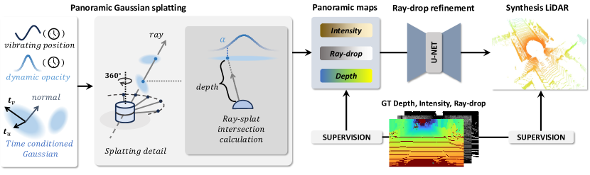
Figure 2: Overview of the GS-LiDAR framework: GS-LiDAR is based on 2D Gaussian primitives with periodic vibration properties, allowing for dynamic modeling of position and opacity along with accurate geometry. At a given timestamp, Gaussians query their states and utilize the proposed panoramic Gaussian splatting technique to render panoramic maps of depth, ray-drop, and intensity. For each ray and Gaussian primitive, we calculate their intersection to obtain the depth and $\alpha$, ensuring more geometrically consistent renderings. The results are subsequently refined by a well-trained U-Net to further enhance the quality of the point clouds.

3.2 Periodic vibration 2D Gaussian

Given the constant presence of moving vehicles and pedestrians in driving scenarios, we aim to utilize a unified representation to model the various objects and elements within the scene. We employ 2D Gaussian primitives (Huang et al., 2024) with periodic vibration properties (Chen et al., 2023a) to accurately capture surface behavior across both space and time. For a 2D Gaussian defined by its central point ${\bm{\mu}}\in\mathbb{R}^{3}$, an opacity parameter $o\in[0,1]$, two principal tangential vectors ${\bm{t}}_{u}\in\mathbb{R}^{3}$ and ${\bm{t}}_{v}\in\mathbb{R}^{3}$, and a scaling vector ${\bm{s}}=(s_{u},s_{v})\in\mathbb{R}^{2}$, we introduce additional learnable attributes that govern the variation of its central point and opacity. These include the vibrating direction ${\bm{v}}\in\mathbb{R}^{3}$, life peak $\tau\in\mathbb{R}$, and time decay rate $\beta\in\mathbb{R}$:

$$\tilde{{\bm{\mu}}}(t) ={\bm{\mu}}+\frac{l}{2\pi}\cdot\sin(\frac{2\pi(t-\tau)}{l})\cdot{\bm{v}},$$ (3)

$$\tilde{o}(t) =o\cdot\exp(-\frac{1}{2}(t-\tau)^{2}\beta^{-2}),$$ (4)

where $\tilde{{\bm{\mu}}}(t)$ represents the vibrating motion around ${\bm{\mu}}$ and $\tau$, and $\tilde{o}(t)$ represents the decayed opacity. The hyper-parameter $l$ denotes the cycle length, which serves as a prior for the scene. Each equipped with a simple motion, the Gaussian primitives can join up to represent any complex motion of dynamic elements in a relay manner. The influence $\mathcal{G}$ of each 2D Gaussian disk is defined within its local tangent plane in world space:

$$\mathcal{G}(u,v)=\exp\left(-\frac{u^{2}+v^{2}}{2}\right),$$ (5)

where $(u,v)$ are the coordinates within the local tangent plane space (UV space). The transformation from UV space to screen space is parameterized as:

$${\bm{x}}(u,v)={\bm{W}}(\tilde{{\bm{\mu}}}(t)+s_{u}{\bm{t}}_{u}u+s_{v}{\bm{t}}_{v}v)={\bm{W}}{\bm{H}}(u,v,1)^{\top},$$ (6)

$$\text{where}\,{\bm{H}}=\begin{bmatrix}s_{u}{\bm{t}}_{u}&s_{v}{\bm{t}}_{v}&\tilde{{\bm{\mu}}}(t)\\ 0&0&1\\ \end{bmatrix}\in\mathbb{R}^{4\times 3}.$$ (7)

Here, ${\bm{W}}\in\mathbb{R}^{4\times 4}$ represents the view transformation matrix, and ${\bm{x}}=(x,y,z,1)^{\top}$ denotes the homogeneous coordinates in sensor space.

3.3 Panoramic Gaussian splatting

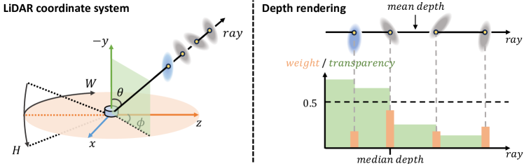
Figure 3: Our LiDAR coordinate system and two ways of depth rendering. The mean depth refers to the weighted average of each depth using the rendering weights, while the median depth is defined as the maximum depth with transparency, i.e., $\prod_{j=1}^{k-1}(1-o_{j}\,\mathcal{G}_{j})$, no greater than 0.5.

LiDAR emits laser pulses and measures the time-of-flight (ToF) to determine object distances, as well as the intensity of reflected light. Spinning LiDAR provides a 360-degree horizontal field of view $(-\pi,\pi)$ and a limited vertical field of view $(\mathrm{VFOV}_{\min},\mathrm{VFOV}_{\max})$, allowing it to perceive the environment with a specific angular resolution. The angular configuration within the LiDAR coordinate system is depicted in Figure 3. Given the pixel coordinates of a point on the range image $(\xi,\eta)$, the corresponding radian angles can be computed using the following equation:

$$\begin{pmatrix}\phi\\ \theta\end{pmatrix}=\begin{pmatrix}(2\xi-W)\pi W^{-1}\\ \eta H^{-1}(\mathrm{VFOV}_{\max}-\mathrm{VFOV}_{\min})+\mathrm{VFOV}_{\min}\end{pmatrix},$$ (8)

where $(W,H)$ represent the width and height of the range image, respectively. A homogeneous point in the LiDAR coordinate system can then be determined from $(\phi,\theta)$ as follows: ${\bm{x}}=(x,y,z,1)^{\top}=(r\sin\theta\sin\phi,-r\cos\theta,r\sin\theta\cos\phi,1)^{\top}$, where $r=\sqrt{x^{2}+y^{2}+z^{2}}$ denotes the distance from the point to the center of the LiDAR.

Ray-splat intersection

We define the ray as the intersection of two orthogonal homogeneous planes, ${\bm{h}}_{x}=(\cos\phi,0,-\sin\phi,0)^{\top}$ and ${\bm{h}}_{y}=(\cos\theta\sin\phi,\sin\theta,\cos\theta\cos\phi,0)^{\top}$, characterized by their normal vectors. These satisfy the conditions ${\bm{h}}_{x}^{\top}{\bm{x}}=0$ and ${\bm{h}}_{y}^{\top}{\bm{x}}=0$. Consequently, given the ray angles $(\phi,\theta)$, the ray-splat intersection $(u,v)$ is determined by solving the following linear equations:

$$\begin{bmatrix}{\bm{h}}_{x},{\bm{h}}_{y}\end{bmatrix}^{\top}{\bm{W}}{\bm{H}}(u,v,1)^{\top}=0.$$ (9)

Let $\begin{bmatrix}{\bm{R}},{\bm{h}}\end{bmatrix}=\begin{bmatrix}{\bm{h}}_{x},{\bm{h}}_{y}\end{bmatrix}^{\top}{\bm{W}}{\bm{H}}$, where ${\bm{R}}\in\mathbb{R}^{2\times 2}$ and ${\bm{h}}\in\mathbb{R}^{2}$, From this, we can solve for $u$ and $v$ as follows:

$$\begin{pmatrix}u\\ v\end{pmatrix}=-{\bm{R}}^{-1}{\bm{h}}.$$ (10)

3.4 LiDAR rendering

In the novel LiDAR view synthesis task, LiDAR point clouds, which include intensity values, can be projected to panoramic range maps and intensity maps. To simulate LiDAR point clouds, we assign each Gaussian a view-dependent intensity value $\lambda$ and a view-dependent ray-drop probability $\rho$, both of which are modeled using spherical harmonics.

Depth map

Considering the ray-splat intersection within the LiDAR coordinate system, the depth value corresponds to the distance $r$ from the intersection point to the center of the LiDAR. Based on Equation 7 and the conversion between $(x,y,z)$ and $(\phi,\theta)$, we have:

$$(r\sin\theta\sin\phi,-r\cos\theta,r\sin\theta\cos\phi,1)^{\top}={\bm{W}}{\bm{H}}(u,v,1)^{\top}.$$ (11)

By multiplying $(\sin\theta\sin\phi,-\cos\theta,\sin\theta\cos\phi,0)$ on both sides, the distance $r$ can be computed as:

$$r=(\sin\theta\sin\phi,-\cos\theta,\sin\theta\cos\phi,0){\bm{W}}{\bm{H}}(u,v,1)^{\top}.$$ (12)

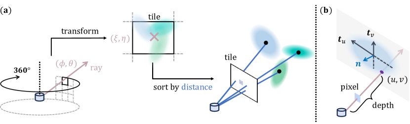
Figure 4: Panoramic Gaussian rasterization details. (a) Our method employs tile-based sorting and rendering. For panoramic ray maps, we first transform the epipolar coordinate system into the pixel coordinate system. The pixel map is then divided into small tiles, and within each tile, Gaussian primitives are sorted based on their distance to the LiDAR origin. (b) During pixel rendering, the $\alpha$ and depth are computed by calculating the intersection between the ray and the Gaussian primitive.

Although we calculate the intersection of each ray with the Gaussian primitives, we still adopt the tile-based rendering method proposed in 3D Gaussian splatting Kerbl et al. (2023) to achieve efficient rendering. As illustrated in Figure 4, we first transform the epipolar coordinates into pixel coordinates and sort the Gaussian primitives within each tile. For pixel rendering, the $\alpha$ and depth are determined based on the intersection results.

During the training process, we utilize both the mean depth and the median depth, and supervise them using the projected ground truth range map as follows:

$$R_{\mathrm{mean}}=\sum^{K}_{k=1}r_{k}\,o_{k}\,\mathcal{G}_{k}\prod_{j=1}^{k-1}(1-o_{j}\,\mathcal{G}_{j}),$$ (13)

$$R_{\mathrm{median}}=\max\left\{r_{k}\Bigg{|}\prod_{j=1}^{k-1}(1-o_{j}\,\mathcal{G}_{j})>0.5\right\},$$ (14)

$$\mathcal{L}_{\mathrm{d}}=\begin{Vmatrix}R_{\mathrm{mean}}-R_{\mathrm{gt}}\end{Vmatrix}_{1}+\begin{Vmatrix}R_{\mathrm{median}}-R_{\mathrm{gt}}\end{Vmatrix}_{1}.$$ (15)

Intensity map

LiDAR intensity refers to the strength of the laser pulse upon its return to the receiver, which is influenced by material properties, surface characteristics, distance, and the incident angle. Intensity data contributes to terrain analysis, facilitates the differentiation of various features, and enhances the classification and precision of point cloud data. Similar to the rendering of mean depth, we aggregate the intensity map $I$ using alpha-blending: $I=\sum^{K}_{k=1}\lambda_{k}\,o_{k}\,\mathcal{G}_{k}\prod_{j=1}^{k-1}(1-o_{j}\,\mathcal{G}_{j})$, which is subsequently supervised by the ground truth intensity:

$$\mathcal{L}_{\mathrm{int}}=\begin{Vmatrix}I-I_{\mathrm{gt}}\end{Vmatrix}_{1}.$$ (16)

Ray-drop probability map

LiDAR ray-drop refers to the phenomenon where some laser pulses do not return to the sensor after striking surfaces, often due to obstructions, absorption by vegetation, or unfavorable angles of incidence. Through alpha-blending, we get a ray-drop probability map from Gaussians: $P_{\mathrm{gs}}=\sum^{K}_{k=1}\rho_{k}\,o_{k}\,\mathcal{G}_{k}\prod_{j=1}^{k-1}(1-o_{j}\,\mathcal{G}_{j})$. Additionally, since the LiDAR ray-drop is also related to the characteristics of the LiDAR itself, we introduce a learnable prior $P_{\mathrm{prior}}$ for the ray-drop. The final ray-drop probability map is expressed as: $P=P_{\mathrm{prior}}+(1-P_{\mathrm{prior}})P_{\mathrm{gs}}$, which is supervised by the ground truth mask using a binary cross-entropy loss:

$$\mathcal{L}_{\mathrm{drop}}=\mathrm{BCE}\left(P,P_{\mathrm{gt}}\right).$$ (17)

However, this modeling of ray-drop does not account for factors such as distance to the sensor, potentially leading to unreliable results. To mitigate this issue, following NeRF-LiDAR (Zhang et al., 2024), we utilize a U-Net (Ronneberger et al., 2015) with residual connections to globally refine the ray-drop mask, thereby preserving consistent patterns across regions. Specifically, the U-Net takes the rendered ray-drop probability map $P$, depth map $R_{\mathrm{mean}}$, and intensity map $I$ as inputs, and outputs the refined ray-drop mask $P_{\mathrm{unet}}$. After training the Gaussians, we continue optimizing the U-Net by supervising the refined ray-drop mask using the same loss function as in Equation 17.

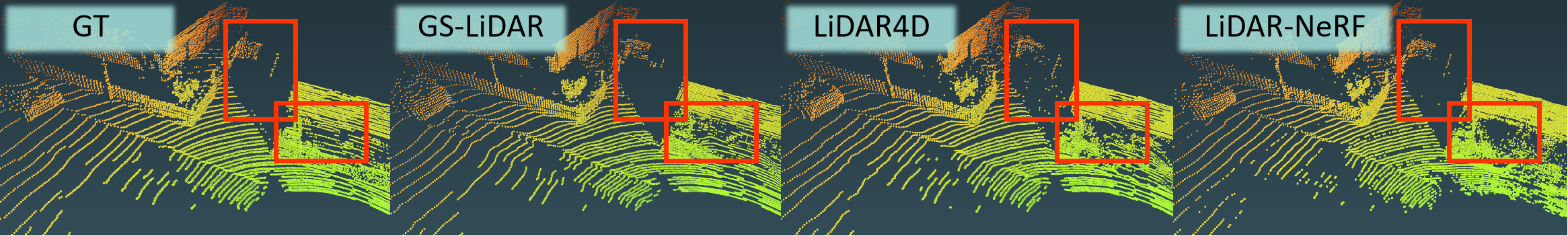
Figure 5: Comparison of 3D LiDAR point cloud. GS-LiDAR produces a more cohesive LiDAR point cloud compared to LiDAR-NeRF (Tao et al., 2023) and LiDAR4D (Zheng et al., 2024). For more results, please refer to the video in our supplementary material.

Table 1: State-of-the-art comparison on KITTI-360 Static Scene Sequence. We color the top results as best and second best.

Method	Point Cloud		Depth					Intensity
	CD$\downarrow$	F-score$\uparrow$	RMSE$\downarrow$	MedAE$\downarrow$	LPIPS$\downarrow$	SSIM$\uparrow$	PSNR$\uparrow$	RMSE$\downarrow$	MedAE$\downarrow$	LPIPS$\downarrow$	SSIM$\uparrow$	PSNR$\uparrow$
LiDARsim (Manivasagam et al., 2020)	2.2249	0.8667	6.5470	0.0759	0.2289	0.7157	21.7746	0.1532	0.0506	0.2502	0.4479	16.3045
NKSR (Huang et al., 2023)	0.5780	0.8685	4.6647	0.0698	0.2295	0.7052	22.5390	0.1565	0.0536	0.2429	0.4200	16.1159
PCGen (Li et al., 2023)	0.2090	0.8597	4.8838	0.1785	0.5210	0.5062	24.3050	0.2005	0.0818	0.6100	0.1248	13.9606
LiDAR-NeRF (Tao et al., 2023)	0.0923	0.9226	3.6801	0.0667	0.3523	0.6043	26.7663	0.1557	0.0549	0.4212	0.2768	16.1683
LiDAR4D (Zheng et al., 2024)	0.0894	0.9264	3.2370	0.0507	0.1313	0.7218	27.8840	0.1343	0.0404	0.2127	0.4698	17.4529
GS-LiDAR (Ours)	0.0847	0.9236	2.8895	0.0411	0.0997	0.8454	28.8807	0.1211	0.0359	0.1630	0.5756	18.3506

3.5 Loss function

To achieve accurate geometry and align the 2D splats with surfaces, we integrate the depth distortion loss and normal consistency loss from 2DGS Huang et al. (2024). Additionally, we employ the chamfer distance loss (Fan et al., 2017) to minimize the disparity between our simulated LiDAR point clouds and the ground truth data.

Depth distortion

The depth distortion loss aims to reduce the distance between ray-splat intersections, encouraging the 2D Gaussian primitives to concentrate on the surface:

$$\mathcal{L}_{\mathrm{dist}}=\sum_{i,j}\omega_{i}\omega_{j}(r_{i}-r_{j})^{2},$$ (18)

where $\omega_{i}$ represents the blending weight of the $i$-th intersection, and $r_{i}$ denotes the depth of the intersection points.

Normal consistency

Since our approach is based on 2D Gaussian primitives, it is crucial to ensure that all 2D splats are locally aligned with the actual surfaces. To achieve this, we align the rendered normal map $\bm{N}$ with the pseudo-normal map $\tilde{\bm{N}}$, which is computed from the gradients of the depth maps:

$$\mathcal{L}_{\mathrm{n}}=1-\bm{N}^{\top}\tilde{\bm{N}}.$$ (19)

Chamfer distance loss

We also incorporate chamfer distance to introduce explicit geometric constraints from the input LiDAR point clouds. By back-projecting both the rendered and ground truth range images into 3D point clouds, ${\bm{S}}_{\mathrm{render}}$ and ${\bm{S}}_{\mathrm{gt}}$, respectively, we minimize the distance between the two point clouds using the chamfer distance (Fan et al., 2017):

$$\mathcal{L}_{\mathrm{ch}}=\mathrm{CD}({\bm{S}}_{\mathrm{render}},{\bm{S}}_{\mathrm{gt}}).$$ (20)

The overall loss function is defined as:

$$\mathcal{L}=\lambda_{\mathrm{d}}\mathcal{L}_{\mathrm{d}}+\lambda_{\mathrm{int}}\mathcal{L}_{\mathrm{int}}+\lambda_{\mathrm{drop}}\mathcal{L}_{\mathrm{drop}}+\lambda_{\mathrm{dist}}\mathcal{L}_{\mathrm{dist}}+\lambda_{\mathrm{n}}\mathcal{L}_{\mathrm{n}}+\lambda_{\mathrm{ch}}\mathcal{L}_{\mathrm{ch}}.$$ (21)

4 Experiment

Table 2: State-of-the-art comparison on KITTI-360 dataset. We color the top results as best and second best.

Method	Point Cloud		Depth					Intensity
	CD$\downarrow$	F-score$\uparrow$	RMSE$\downarrow$	MedAE$\downarrow$	LPIPS$\downarrow$	SSIM$\uparrow$	PSNR$\uparrow$	RMSE$\downarrow$	MedAE$\downarrow$	LPIPS$\downarrow$	SSIM$\uparrow$	PSNR$\uparrow$
LiDARsim (Manivasagam et al., 2020)	3.2228	0.7157	6.9153	0.1279	0.2926	0.6342	21.4608	0.1666	0.0569	0.3276	0.3502	15.5853
NKSR (Huang et al., 2023)	1.8982	0.6855	5.8403	0.0996	0.2752	0.6409	23.0368	0.1742	0.0590	0.3337	0.3517	15.2081
PCGen (Li et al., 2023)	0.4636	0.8023	5.6583	0.2040	0.5391	0.4903	23.1675	0.1970	0.0763	0.5926	0.1351	14.1181
LiDAR-NeRF (Tao et al., 2023)	0.1438	0.9091	4.1753	0.0566	0.2797	0.6568	25.9878	0.1404	0.0443	0.3135	0.3831	17.1549
D-NeRF (Pumarola et al., 2021)	0.1442	0.9128	4.0194	0.0508	0.3061	0.6634	26.2344	0.1369	0.0440	0.3409	0.3748	17.3554
TiNeuVox-B (Fang et al., 2022)	0.1748	0.9059	4.1284	0.0502	0.3427	0.6514	26.0267	0.1363	0.0453	0.4365	0.3457	17.3535
K-Planes (Fridovich-Keil et al., 2023)	0.1302	0.9123	4.1322	0.0539	0.3457	0.6385	26.0236	0.1415	0.0498	0.4081	0.3008	17.0167
LiDAR4D (Zheng et al., 2024)	0.1089	0.9272	3.5256	0.0404	0.1051	0.7647	27.4767	0.1195	0.0327	0.1845	0.5304	18.5561
GS-LiDAR (Ours)	0.1085	0.9231	3.1212	0.0340	0.0902	0.8553	28.4381	0.1161	0.0313	0.1825	0.5914	18.7482

Table 3: State-of-the-art comparison on nuScenes dataset. The notations are consistent with the KITTI-360 Table 2 above.

Method	Point Cloud		Depth					Intensity
	CD$\downarrow$	F-score$\uparrow$	RMSE$\downarrow$	MedAE$\downarrow$	LPIPS$\downarrow$	SSIM$\uparrow$	PSNR$\uparrow$	RMSE$\downarrow$	MedAE$\downarrow$	LPIPS$\downarrow$	SSIM$\uparrow$	PSNR$\uparrow$
LiDARsim Manivasagam et al. (2020)	12.1383	0.6512	10.5539	0.3572	0.1871	0.5653	17.7841	0.0659	0.0115	0.1160	0.5170	23.7791
NKSR Huang et al. (2023)	11.4910	0.6178	9.3731	0.5763	0.2111	0.5637	18.7774	0.0680	0.0119	0.1290	0.5031	23.4905
PCGen Li et al. (2023)	2.1998	0.6341	8.8364	0.4011	0.1792	0.5440	19.2799	0.0768	0.0147	0.1308	0.4410	22.4428
LiDAR-NeRF Tao et al. (2023)	0.3225	0.8576	7.1566	0.0338	0.0702	0.7188	21.2129	0.0467	0.0076	0.0483	0.7264	26.9927
D-NeRF Pumarola et al. (2021)	0.3296	0.8513	7.1089	0.0368	0.0789	0.7130	21.2594	0.0467	0.0080	0.0492	0.7180	26.9951
TiNeuVox-B Fang et al. (2022)	0.3920	0.8627	7.2093	0.0290	0.1549	0.6873	21.0932	0.0462	0.0080	0.1294	0.7107	26.8620
K-Planes Fridovich-Keil et al. (2023)	0.2982	0.8887	6.7960	0.0209	0.1218	0.7258	21.6203	0.0438	0.0076	0.1127	0.7364	27.4227
LiDAR4D (Zheng et al., 2024)	0.2443	0.8915	6.7831	0.0258	0.0569	0.7396	21.7189	0.0426	0.0071	0.0459	0.7498	27.7977
GS-LiDAR (Ours)	0.2382	0.9055	5.8925	0.0198	0.0708	0.8394	22.2482	0.0415	0.0067	0.0627	0.7291	27.7420

4.1 Experiment setup

Datasets

We conduct extensive experiments on both dynamic and static scenes using the KITTI-360 (Liao et al., 2022) and nuScenes (Caesar et al., 2020) datasets, with the dynamic scenes featuring a significant number of moving vehicles. The KITTI-360 dataset employs a 64-beam LiDAR with a vertical field of view (FOV) of 26.4 degrees and an acquisition frequency of 10Hz. Following LiDAR4D (Zheng et al., 2024), we select 51 consecutive frames as a single scene and hold out 4 samples at 10-frame intervals for novel view synthesis (NVS) evaluation. For the nuScenes dataset, the LiDAR system uses 32 beams with a 40-degree vertical FOV and a 20Hz acquisition frequency. To ensure consistency with KITTI-360, we maintain a sampling frequency of 10Hz.

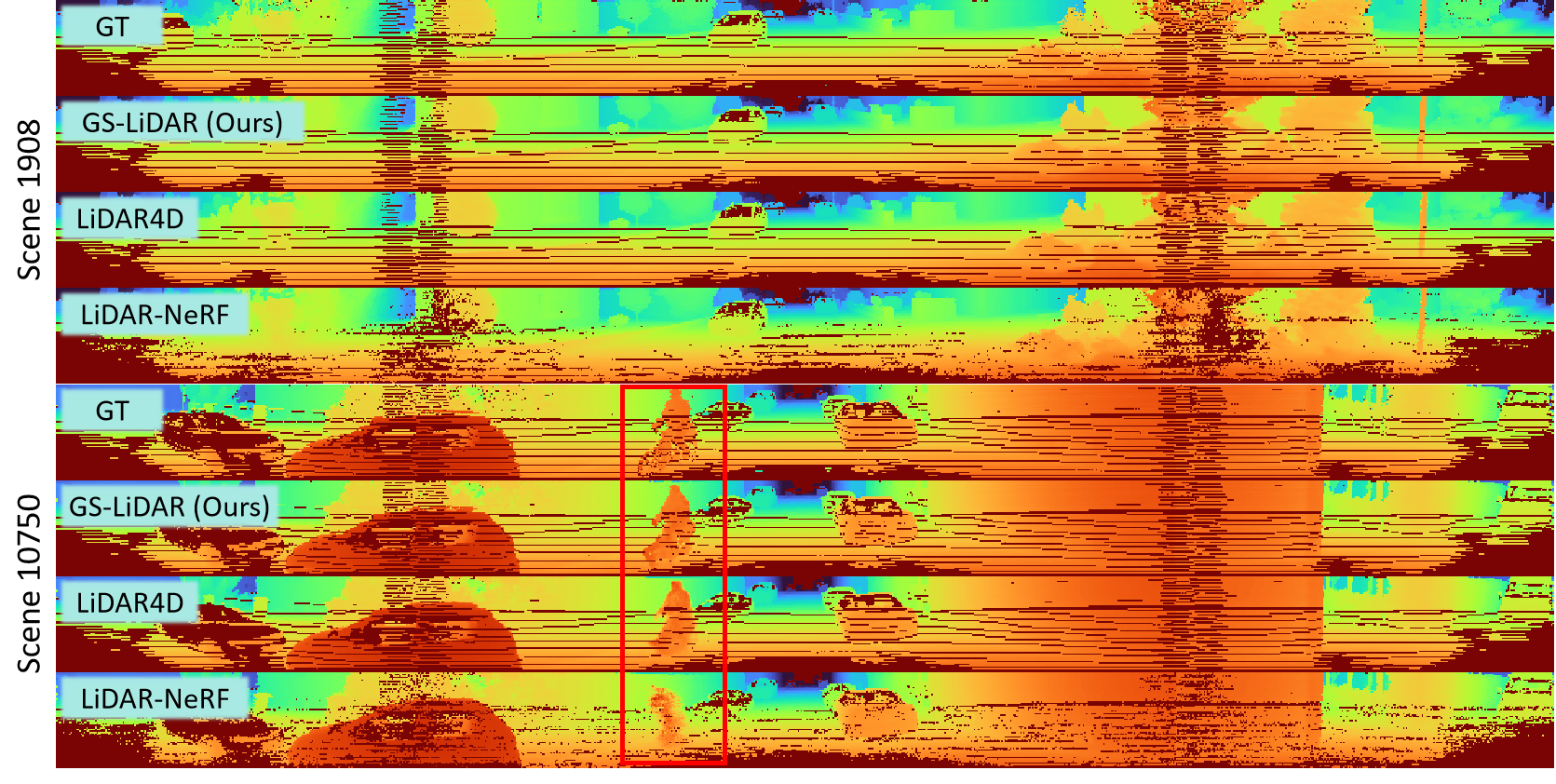
Figure 6: Comparison of the rendered depth map with competitors. For more results, please refer to the video in our supplementary material.

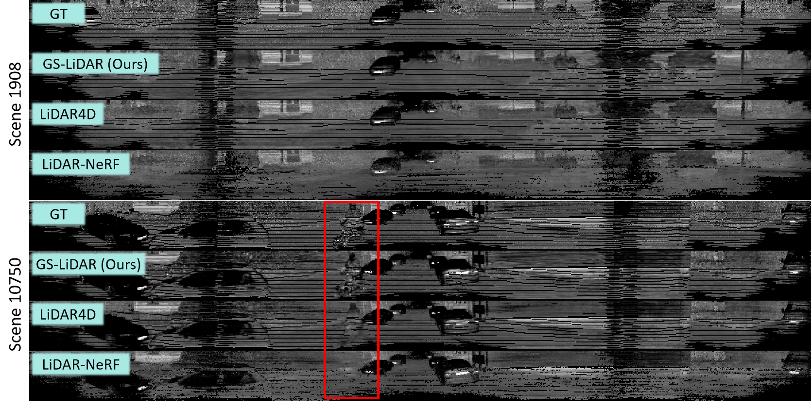
Figure 7: Comparison of the rendered intensity map with competitors.

Competitors

We evaluate our method alongside recent data-driven approaches LiDARsim (Manivasagam et al., 2020) and PCGen (Li et al., 2023). Additionally, we compare our results with the per-scene optimized reconstruction method NKSR (Huang et al., 2023), LiDAR-NeRF (Tao et al., 2023) and the state-of-the-art method, LiDAR4D (Zheng et al., 2024). We also include competitive dynamic neural radiance field methods, such as D-NeRF (Pumarola et al., 2021), K-Planes (Fridovich-Keil et al., 2023), and TiNeuVox (Fang et al., 2022), for comparison.

Metrics

We employ a comprehensive set of evaluation metrics for assessing point cloud, depth, and intensity measurements. Chamfer distance (Fan et al., 2017) is used to quantify the 3D geometric discrepancy between the generated and ground-truth point clouds based on nearest neighbors. Additionally, we report the F-score with a 5cm error threshold. For pixel-level error analysis of projected LiDAR range maps, we introduce Root Mean Square Error (RMSE) and Median Absolute Error (MedAE). Furthermore, we utilize LPIPS (Zhang et al., 2018), SSIM (Wang et al., 2004), and PSNR to assess image-level error on depth and intensity.

Implementation details

We randomly sample $1\times 10^{6}$ LiDAR points for point initialization. For the loss function and regularization terms, we use the following coefficients: $\lambda_{\mathrm{d}}=10$, $\lambda_{\mathrm{int}}=0.05$, $\lambda_{\mathrm{drop}}=0.05$, $\lambda_{\mathrm{dist}}=0.1$, $\lambda_{\mathrm{n}}=0.1$, and $\lambda_{\mathrm{ch}}=0.1$. All experiments are conducted on a single NVIDIA RTX A6000 GPU, with a total of 30,000 iterations, taking approximately 1.5 hours to produce the final results. The rendering speed reaches up to 11 frames per second (FPS).

4.2 Evaluation on static scenes

Table 1 provides the quantitative results for static scenes in KITTI-360 dataset across all methods. GS-LiDAR outperforms the competitors on most metrics. Notably, there is a 5.3% reduction in the Chamfer distance of the simulated point cloud, a 10.7% reduction in the RMSE of simulated depth, and a 9.8% reduction in the RMSE of simulated intensity. As shown in Figure 5, GS-LiDAR produces a more cohesive LiDAR point cloud, which can be attributed to the accurate range maps generated by the proposed panoramic Gaussian splatting technique.

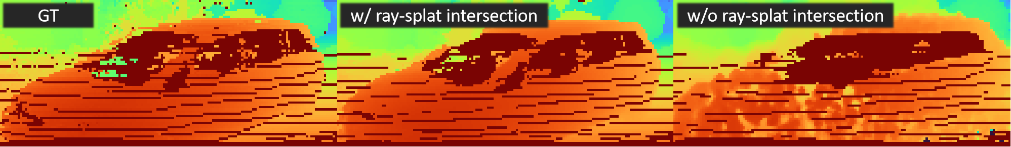
Figure 8: Comparison of w/ and w/o ray-splat intersection.

Table 4: Ablation studies on various components of GS-LiDAR.

Method	Point Cloud		Depth					Intensity
	CD$\downarrow$	F-score$\uparrow$	RMSE$\downarrow$	MedAE$\downarrow$	LPIPS$\downarrow$	SSIM$\uparrow$	PSNR$\uparrow$	RMSE$\downarrow$	MedAE$\downarrow$	LPIPS$\downarrow$	SSIM$\uparrow$	PSNR$\uparrow$
GS-LiDAR	0.1085	0.9231	3.1212	0.0340	0.0902	0.8553	28.4381	0.1161	0.0313	0.1825	0.5914	18.7482
w/o ray-splat intersection	3.1605	0.5091	6.6871	0.2367	0.4828	0.5754	21.5918	0.2320	0.1170	0.5166	0.1976	12.7069
w/o periodic vibration	0.1333	0.9100	3.1738	0.0359	0.0946	0.8577	28.2876	0.1162	0.0342	0.2166	0.5849	18.7288
w/o median depth loss	0.1254	0.9125	3.1414	0.0347	0.0941	0.8574	28.3567	0.1163	0.0313	0.1831	0.5902	18.7262
w/o depth distortion loss	0.1237	0.9229	3.2016	0.0341	0.0908	0.8567	28.2854	0.1176	0.0314	0.1842	0.5833	18.7078
w/o normal consistency loss	0.1158	0.9230	3.1993	0.0344	0.0908	0.8556	28.3852	0.1165	0.0314	0.1850	0.5887	18.7085
w/o chamfer distance loss	0.1152	0.9227	3.1354	0.0341	0.0907	0.8559	28.3892	0.1167	0.0341	0.1811	0.5911	18.7383
w/o ray-drop refinement	0.1121	0.9223	4.0791	0.0424	0.1952	0.7433	26.1083	0.1346	0.0384	0.2477	0.4569	17.4541

4.3 Evaluation on dynamic scenes

To further validate the effectiveness of GS-LiDAR, we conduct LiDAR synthesis evaluations on dynamic scenes from the KITTI-360 and nuScenes datasets. For the KITTI-360 dataset, as shown in Table 2, our method demonstrates superior performance, achieving a 0.3% reduction in chamfer distance for simulated point cloud, a 11.4% reduction in RMSE for simulated depth, and a 2.8% reduction in RMSE for simulated intensity. As illustrated in Figure 6 and Figure 7, GS-LiDAR achieves significantly better visual quality in simulated depth and intensity maps compared to competitors. This improvement is primarily due to the use of 2D Gaussian primitives with periodic vibration properties, enabling precise modeling of both static and dynamic geometries. For the nuScenes dataset, as shown in Table 3, GS-LiDAR also showcases notable performance, with a 2.5% reduction in chamfer distance for simulated point cloud, a 13.1% reduction in RMSE for simulated depth, and a 2.6% reduction in RMSE for simulated intensity.

4.4 Ablation study

We provide quantitative ablation studies on various components of GS-LiDAR in Table 4. As shown in Figure 8, we find that the use of ray-splat intersection enhances the capability of GS-LiDAR in modeling the surface of the scene. For the “w/o ray-splat intersection” case, we implement a basic 3D Gaussian splatting approach by adapting the projection calculation method specifically for panoramic maps. The integration of periodic vibration properties further improves GS-LiDAR’s capability in handling dynamic elements. Regularization terms, including median depth loss, depth distortion loss, and chamfer distance loss, contribute to the improved quality of the simulated LiDAR point clouds. Additionally, the ray-drop refinement technique improves the accuracy of the ray-drop mask, resulting in substantial gains in the metrics for simulated depth and intensity.

5 Conclusion

We present GS-LiDAR, a novel framework designed to generate realistic LiDAR point clouds. To uniformly model the accurate surface of various elements in driving scenarios, we employ 2D Gaussian primitives with periodic vibration properties. Furthermore, we propose a novel panoramic Gaussian splatting technique with explicit ray-splat intersection for fast and efficient rendering of panoramic depth maps. By incorporating intensity and ray-drop SH coefficients into the Gaussian primitives, we enhance the realism of the rendered point clouds, making them more closely resemble actual LiDAR data. Our method significantly surpasses previous NeRF-based approaches in both computational speed and simulation quality on the KITTI-360 and nuScenes datasets.

References

- Barron et al. (2021) Jonathan T. Barron, Ben Mildenhall, Matthew Tancik, Peter Hedman, Ricardo Martin-Brualla, and Pratul P. Srinivasan. Mip-nerf: A multiscale representation for anti-aliasing neural radiance fields. In ICCV, 2021.
- Barron et al. (2022) Jonathan T. Barron, Ben Mildenhall, Dor Verbin, Pratul P. Srinivasan, and Peter Hedman. Mip-nerf 360: Unbounded anti-aliased neural radiance fields. In CVPR, 2022.
- Barron et al. (2023) Jonathan T Barron, Ben Mildenhall, Dor Verbin, Pratul P Srinivasan, and Peter Hedman. Zip-nerf: Anti-aliased grid-based neural radiance fields. In ICCV, 2023.
- Caesar et al. (2020) Holger Caesar, Varun Bankiti, Alex H Lang, Sourabh Vora, Venice Erin Liong, Qiang Xu, Anush Krishnan, Yu Pan, Giancarlo Baldan, and Oscar Beijbom. nuscenes: A multimodal dataset for autonomous driving. In CVPR, 2020.
- Chen et al. (2022) Anpei Chen, Zexiang Xu, Andreas Geiger, Jingyi Yu, and Hao Su. Tensorf: Tensorial radiance fields. In ECCV, 2022.
- Chen et al. (2023a) Yurui Chen, Chun Gu, Junzhe Jiang, Xiatian Zhu, and Li Zhang. Periodic vibration gaussian: Dynamic urban scene reconstruction and real-time rendering. arXiv preprint, 2023a.
- Chen et al. (2023b) Zhang Chen, Zhong Li, Liangchen Song, Lele Chen, Jingyi Yu, Junsong Yuan, and Yi Xu. Neurbf: A neural fields representation with adaptive radial basis functions. In ICCV, 2023b.
- Chen et al. (2023c) Zhiqin Chen, Thomas Funkhouser, Peter Hedman, and Andrea Tagliasacchi. Mobilenerf: Exploiting the polygon rasterization pipeline for efficient neural field rendering on mobile architectures. In CVPR, 2023c.
- Dosovitskiy et al. (2017) Alexey Dosovitskiy, German Ros, Felipe Codevilla, Antonio Lopez, and Vladlen Koltun. Carla: An open urban driving simulator. In CoRL, 2017.
- Fan et al. (2017) Haoqiang Fan, Hao Su, and Leonidas J Guibas. A point set generation network for 3d object reconstruction from a single image. In CVPR, 2017.
- Fang et al. (2022) Jiemin Fang, Taoran Yi, Xinggang Wang, Lingxi Xie, Xiaopeng Zhang, Wenyu Liu, Matthias Nießner, and Qi Tian. Fast dynamic radiance fields with time-aware neural voxels. In SIGGRAPH Asia, 2022.
- Fridovich-Keil et al. (2022) Sara Fridovich-Keil, Alex Yu, Matthew Tancik, Qinhong Chen, Benjamin Recht, and Angjoo Kanazawa. Plenoxels: Radiance fields without neural networks. In CVPR, 2022.
- Fridovich-Keil et al. (2023) Sara Fridovich-Keil, Giacomo Meanti, Frederik Rahbæk Warburg, Benjamin Recht, and Angjoo Kanazawa. K-planes: Explicit radiance fields in space, time, and appearance. In CVPR, 2023.
- Gao et al. (2024) Jian Gao, Chun Gu, Youtian Lin, Hao Zhu, Xun Cao, Li Zhang, and Yao Yao. Relightable 3d gaussian: Real-time point cloud relighting with brdf decomposition and ray tracing. In ECCV, 2024.
- Guillard et al. (2022) Benoît Guillard, Sai Vemprala, Jayesh K Gupta, Ondrej Miksik, Vibhav Vineet, Pascal Fua, and Ashish Kapoor. Learning to simulate realistic lidars. In IROS, 2022.
- Hedman et al. (2021) Peter Hedman, Pratul P Srinivasan, Ben Mildenhall, Jonathan T Barron, and Paul Debevec. Baking neural radiance fields for real-time view synthesis. In ICCV, 2021.
- Hu et al. (2023) Wenbo Hu, Yuling Wang, Lin Ma, Bangbang Yang, Lin Gao, Xiao Liu, and Yuewen Ma. Tri-miprf: Tri-mip representation for efficient anti-aliasing neural radiance fields. In ICCV, 2023.
- Huang et al. (2024) Binbin Huang, Zehao Yu, Anpei Chen, Andreas Geiger, and Shenghua Gao. 2d gaussian splatting for geometrically accurate radiance fields. In ACM SIGGRAPH, 2024.
- Huang et al. (2023) Jiahui Huang, Zan Gojcic, Matan Atzmon, Or Litany, Sanja Fidler, and Francis Williams. Neural kernel surface reconstruction. In CVPR, 2023.
- Kerbl et al. (2023) Bernhard Kerbl, Georgios Kopanas, Thomas Leimkühler, and George Drettakis. 3d gaussian splatting for real-time radiance field rendering. ACM TOG, 2023.
- Koenig & Howard (2004) Nathan Koenig and Andrew Howard. Design and use paradigms for gazebo, an open-source multi-robot simulator. In IROS, 2004.
- Li et al. (2023) Chenqi Li, Yuan Ren, and Bingbing Liu. Pcgen: Point cloud generator for lidar simulation. In ICRA, 2023.
- Liao et al. (2022) Yiyi Liao, Jun Xie, and Andreas Geiger. Kitti-360: A novel dataset and benchmarks for urban scene understanding in 2d and 3d. IEEE TPAMI, 2022.
- Liu et al. (2020) Lingjie Liu, Jiatao Gu, Kyaw Zaw Lin, Tat-Seng Chua, and Christian Theobalt. Neural sparse voxel fields. NeurIPS, 2020.
- Manivasagam et al. (2020) Sivabalan Manivasagam, Shenlong Wang, Kelvin Wong, Wenyuan Zeng, Mikita Sazanovich, Shuhan Tan, Bin Yang, Wei-Chiu Ma, and Raquel Urtasun. Lidarsim: Realistic lidar simulation by leveraging the real world. In CVPR, 2020.
- Mildenhall et al. (2020) Ben Mildenhall, Pratul P Srinivasan, Matthew Tancik, Jonathan T Barron, Ravi Ramamoorthi, and Ren Ng. Nerf: Representing scenes as neural radiance fields for view synthesis. In ECCV, 2020.
- Müller et al. (2022) Thomas Müller, Alex Evans, Christoph Schied, and Alexander Keller. Instant neural graphics primitives with a multiresolution hash encoding. ACM TOG, 2022.
- Pumarola et al. (2021) Albert Pumarola, Enric Corona, Gerard Pons-Moll, and Francesc Moreno-Noguer. D-nerf: Neural radiance fields for dynamic scenes. In CVPR, 2021.
- Reiser et al. (2021) Christian Reiser, Songyou Peng, Yiyi Liao, and Andreas Geiger. Kilonerf: Speeding up neural radiance fields with thousands of tiny mlps. In ICCV, 2021.
- Reiser et al. (2023) Christian Reiser, Rick Szeliski, Dor Verbin, Pratul Srinivasan, Ben Mildenhall, Andreas Geiger, Jon Barron, and Peter Hedman. Merf: Memory-efficient radiance fields for real-time view synthesis in unbounded scenes. ACM TOG, 2023.
- Ronneberger et al. (2015) Olaf Ronneberger, Philipp Fischer, and Thomas Brox. U-net: Convolutional networks for biomedical image segmentation. In MICCAI, 2015.
- Shah et al. (2018) Shital Shah, Debadeepta Dey, Chris Lovett, and Ashish Kapoor. Airsim: High-fidelity visual and physical simulation for autonomous vehicles. In Field and Service Robotics: Results of the 11th International Conference, 2018.
- Sun et al. (2022) Cheng Sun, Min Sun, and Hwann-Tzong Chen. Direct voxel grid optimization: Super-fast convergence for radiance fields reconstruction. In CVPR, 2022.
- Tao et al. (2023) Tang Tao, Longfei Gao, Guangrun Wang, Peng Chen, Dayang Hao, Xiaodan Liang, Mathieu Salzmann, and Kaicheng Yu. Lidar-nerf: Novel lidar view synthesis via neural radiance fields. arXiv preprint, 2023.
- Tao et al. (2024) Tang Tao, Guangrun Wang, Yixing Lao, Peng Chen, Jie Liu, Liang Lin, Kaicheng Yu, and Xiaodan Liang. Alignmif: Geometry-aligned multimodal implicit field for lidar-camera joint synthesis. In CVPR, 2024.
- Wang et al. (2004) Zhou Wang, Alan C Bovik, Hamid R Sheikh, and Eero P Simoncelli. Image quality assessment: from error visibility to structural similarity. IEEE TIP, 2004.
- Wu et al. (2024) Hanfeng Wu, Xingxing Zuo, Stefan Leutenegger, Or Litany, Konrad Schindler, and Shengyu Huang. Dynamic lidar re-simulation using compositional neural fields. In CVPR, 2024.
- Xie et al. (2023a) Tianyi Xie, Zeshun Zong, Yuxing Qiu, Xuan Li, Yutao Feng, Yin Yang, and Chenfanfu Jiang. Physgaussian: Physics-integrated 3d gaussians for generative dynamics. arXiv preprint, 2023a.
- Xie et al. (2023b) Ziyang Xie, Junge Zhang, Wenye Li, Feihu Zhang, and Li Zhang. S-nerf: Neural radiance fields for street views. In ICLR, 2023b.
- Xue et al. (2024) Weiyi Xue, Zehan Zheng, Fan Lu, Haiyun Wei, Guang Chen, and Changjun Jiang. Geonlf: Geometry guided pose-free neural lidar fields. arXiv preprint, 2024.
- Yan et al. (2024) Yunzhi Yan, Haotong Lin, Chenxu Zhou, Weijie Wang, Haiyang Sun, Kun Zhan, Xianpeng Lang, Xiaowei Zhou, and Sida Peng. Street gaussians for modeling dynamic urban scenes. In ECCV, 2024.
- Yang et al. (2024a) Jiawei Yang, Boris Ivanovic, Or Litany, Xinshuo Weng, Seung Wook Kim, Boyi Li, Tong Che, Danfei Xu, Sanja Fidler, Marco Pavone, et al. Emernerf: Emergent spatial-temporal scene decomposition via self-supervision. In ICLR, 2024a.
- Yang et al. (2024b) Zeyu Yang, Hongye Yang, Zijie Pan, Xiatian Zhu, and Li Zhang. Real-time photorealistic dynamic scene representation and rendering with 4d gaussian splatting. In ICLR, 2024b.
- Yariv et al. (2023) Lior Yariv, Peter Hedman, Christian Reiser, Dor Verbin, Pratul P. Srinivasan, Richard Szeliski, Jonathan T. Barron, and Ben Mildenhall. Bakedsdf: Meshing neural sdfs for real-time view synthesis. arXiv preprint, 2023.
- Yu et al. (2021) Alex Yu, Ruilong Li, Matthew Tancik, Hao Li, Ren Ng, and Angjoo Kanazawa. PlenOctrees for real-time rendering of neural radiance fields. In ICCV, 2021.
- Zhang et al. (2024) Junge Zhang, Feihu Zhang, Shaochen Kuang, and Li Zhang. Nerf-lidar: Generating realistic lidar point clouds with neural radiance fields. In AAAI, 2024.
- Zhang et al. (2018) Richard Zhang, Phillip Isola, Alexei A Efros, Eli Shechtman, and Oliver Wang. The unreasonable effectiveness of deep features as a perceptual metric. In CVPR, 2018.
- Zheng et al. (2024) Zehan Zheng, Fan Lu, Weiyi Xue, Guang Chen, and Changjun Jiang. Lidar4d: Dynamic neural fields for novel space-time view lidar synthesis. In CVPR, 2024.
- Zielonka et al. (2023) Wojciech Zielonka, Timur Bagautdinov, Shunsuke Saito, Michael Zollhöfer, Justus Thies, and Javier Romero. Drivable 3d gaussian avatars. arXiv preprint, 2023.