Efficient Mitigation of Error Floors in Quantum Error Correction using Non-Binary Low-Density Parity-Check Codes

Abstract

In this paper, we propose an efficient method to reduce error floors in quantum error correction using non-binary low-density parity-check (LDPC) codes. We identify and classify cycle structures in the parity-check matrix where estimated noise becomes trapped, and develop tailored decoding methods for each cycle type. For Type-I cycles, we propose a method to make the difference between estimated and true noise degenerate. Type-II cycles are shown to be uncorrectable, while for Type-III cycles, we utilize the fact that cycles in non-binary LDPC codes do not necessarily correspond to codewords, allowing us to estimate the true noise. Our method significantly improves decoding performance and reduces error floors.

I Introduction

Recent advancements in quantum computing have made it possible to develop systems with tens of reliable logical qubits, constructed from thousands of noisy physical qubits [1]. However, many key applications of quantum computers require quantum computations involving millions, or even more, logical qubits [2]. This highlights the urgent need for highly efficient quantum error correction techniques capable of supporting such large-scale logical qubit systems.

In [3], a generalization of the construction method of $(J=2,L)$-regular non-binary low-density parity-check (LDPC) codes from [4] was proposed, where the sum-product (SP) algorithm was applied to simultaneously decode X and Z errors in quantum codes. The method achieves performance close to the hashing bound while maintaining scalability and ensuring a constant coding rate as the code length increases.

For small values of $L$, the existence of cycles of length $2L$ in the parity-check matrices causes the SP algorithm to fail in estimating the noise exactly, resulting in a high error floor. In quantum codes, even if the estimated noise $\hat{E}$ does not exactly match the true noise $E$, if $\hat{E}^{\dagger}E$ forms a degenerate error, the codeword can still be recovered. Using this property, this paper explores an efficient method for searching for $\hat{E}$ such that $\hat{E}^{\dagger}E$ forms a degenerate error, for the codes in [3] and [4].

In this paper, we propose a method to reduce the error floor by applying postprocessing with a computational complexity independent of the code length. First, we identify the cycle structures in the parity-check matrix where the estimated noise, which causes the error floor, becomes trapped. We then classify these cycles into three types and propose a decoding method based on this classification. For Type-I cycles, we propose a method to determine the estimated noise such that the difference between the estimated noise and the true noise becomes degenerate. It is shown that Type-II cycles cannot be corrected. For Type-III cycles, we use the fact that in the case of non-binary codes, unlike the binary case, cycles in $(J=2,L)$-regular codes do not necessarily correspond to codewords. Based on this, we propose a method to estimate the true noise.

II Preparation

The Pauli group $\mathcal{P}_{n}$ is non-commutative; however, by ignoring the global phase factor $\alpha$ of Pauli operators, we obtain the quotient group $\mathcal{P}_{n}/\{\pm I,\pm iI\}$, which is the subgroup $\{\pm I,\pm iI\}\subset\mathcal{P}_{n}$ modulo. Here, $I$ represents the identity operator on the space $\mathbb{C}^{2^{n}}$. This quotient group is isomorphic to the commutative group $\mathbb{Z}_{2}^{2n}$, and the isomorphism for $E\in\mathcal{P}_{n}/\{\pm I,\pm iI\}$ is given as follows:

$$E=\alpha\bigotimes_{i=1}^{n}X^{x_{i}}Z^{z_{i}}\leftrightarrow(\underline{x}|\underline{z})=\left(x_{1},\ldots,x_{n}\mid z_{1},\ldots,z_{n}\right).$$ (1)

Using this correspondence, we identify the Pauli error $E$ with its binary representation $(\underline{x}|\underline{z})$. Whether the vector is a row vector or column vector should be understood from the context.

A very important subclass of stabilizer codes [5] is the CSS codes [6, 7]. CSS codes are a type of stabilizer code characterized by the property that the non-identity components of each stabilizer generator within a tensor product are all equal to $X$ or all equal to $Z$.

The check matrix of the stabilizer group $S$ is expressed as binary vectors arranged in rows. Without loss of generality, the check matrix $H$ of a CSS code of length $n$ can be expressed as follows:

$$H=\begin{pmatrix}H_{X}&O\\ O&H_{Z}\end{pmatrix}\in\mathbb{F}_{2}^{(m_{X}+m_{Z})\times 2n},$$ (2)

where $H_{X},H_{Z}$ are binary matrices of sizes $m_{X}\times n$ and $m_{Z}\times n$, respectively. The commutativity of the stabilizer generators implies that $H_{X}H_{Z}^{\mathsf{T}}=O$. For simplicity, this paper assumes $m=m_{X}=m_{Z}$. The condition $H_{X}H_{Z}^{\mathsf{T}}=O$ is equivalent to the following:

$$C_{Z}^{\perp}\subset C_{X},\quad C_{X}^{\perp}\subset C_{Z},$$ (3)

where $C_{X},C_{Z}$ are the code spaces defined by $H_{X},H_{Z}$ when considered as parity-check matrices. Furthermore, the dimension $k$ of the CSS code of length $n$ can be determined by the following formula:

$$k=n-\operatorname{rank}H_{X}-\operatorname{rank}H_{Z}.$$

Let us consider the codeword state $|\psi\rangle$ with a Pauli error $E\leftrightarrow(\underline{x},\underline{z})$ applied, resulting in the state $E|\psi\rangle$. The decoder considered in this paper performs decoding according to the following steps:

1. Measure the syndrome $(\underline{s}=H_{Z}\underline{x},\underline{t}=H_{X}\underline{z})\in\mathbb{F}_{2}^{2m}$.

2. Based on the syndrome, estimate the noise as $\hat{E}\leftrightarrow(\underline{\hat{x}},\underline{\hat{z}})$ that satisfies the following:

   $$H_{X}\underline{\hat{z}}=\underline{s},\quad H_{Z}\underline{\hat{x}}=\underline{t}$$ (4)

3. The codeword $|\psi\rangle$ is affected by noise $E$, resulting in the state $E|\psi\rangle$. Applying $\hat{E}^{\dagger}$ to this state yields $E^{\dagger}E|\psi\rangle$. If $\hat{E}^{\dagger}E\in S$, then $\hat{E}^{\dagger}E|\psi\rangle\propto|\psi\rangle$, and the codeword is recovered.

The condition $\hat{E}^{\dagger}E\in S$ is equivalent to the existence of $\underline{a}=(a_{1},\ldots,a_{2m})^{\mathsf{T}}\in\mathbb{F}_{2}^{2m}$ such that $\prod_{i=1}^{m}S_{i}^{a_{i}}=\hat{E}^{\dagger}E$, where $S_{i}$ are the stabilizer generators for $i=1,\ldots,2m$. Moreover, since $\hat{E}^{\dagger}E\leftrightarrow(\underline{x}+\underline{\hat{x}}|\underline{z}+\underline{\hat{z}})$, this is equivalent to:

$$\sum_{i=1}^{m}{a_{i}}\underline{s}_{i}=(\underline{x}+\underline{\hat{x}}|\underline{z}+\underline{\hat{z}}),\quad\text{for }i=1,\ldots,m,$$ (5)

where $S_{i}\leftrightarrow\underline{s}_{i}$. Writing this in terms of matrices and vectors, we get $H^{\mathsf{T}}\underline{a}=(\underline{x}+\underline{\hat{x}}|\underline{z}+\underline{\hat{z}})$. Specifically, for CSS codes, since the parity-check matrix is given by (2), we use $\underline{a}=(\underline{a}_{X}|\underline{a}_{Z})$ to obtain:

$$(H_{X})^{\mathsf{T}}\underline{a}_{X}=\underline{x}+\underline{\hat{x}},\quad(H_{Z})^{\mathsf{T}}\underline{a}_{Z}=\underline{z}+\underline{\hat{z}}$$ (6)

which is equivalent to each of (7) and (8):

$$G_{X}\left(\underline{x}+\underline{\hat{x}}\right)=0,\quad G_{Z}\left(\underline{z}+\underline{\hat{z}}\right)=0,$$ (7)

$$\underline{\hat{x}}+\underline{x}\in C_{X}^{\perp},\quad\underline{\hat{z}}+\underline{z}\in C_{Z}^{\perp},$$ (8)

where $G_{X},G_{Z}$ are generator matrices of $H_{X},H_{Z}$, respectively.

From (3), it follows that (8) implies

$$H_{X}\left(\underline{z}+\underline{\hat{z}}\right)=0,\quad H_{Z}\left(\underline{x}+\underline{\hat{x}}\right)=0,$$ (9)

which is equivalent to (4). The following is sufficient for (8):

$$\underline{x}+\underline{\hat{x}}=H_{X}^{(i)},\quad\underline{z}+\underline{\hat{z}}=H_{Z}^{(i^{\prime})}$$ (10)

for some $i,i^{\prime},$where $H_{Z}^{(i)},H_{X}^{(i^{\prime})}$ are the $i$-th and $i^{\prime}$-th row vectors of $H_{Z}$ and $H_{X}$, respectively.

III Code Construction

In this paper, the primary target code uses the parameters $J=2,L=6,q=2^{e}$, and $e=8$. Codes with varying values of the parameter $L$ are used as comparisons. Let $N=LP$, $M=JP$, $n=eN$, and $m=eM$. The finite field of size $q$ is denoted as $\mathbb{F}_{q}$. Using the methods proposed in [4] and [3], $H_{X}$ and $H_{Z}$ are constructed through the following outline steps.

1. Generate a pair of orthogonal $\mathbb{F}_{2}$-valued $(J=2,L,P)$ protograph matrices $(\hat{H}_{X},\hat{H}_{Z})\in(\mathbb{F}_{2}^{M\times N})^{2}$ such that the girth is 12.

2. Generate a pair of orthogonal $\mathbb{F}_{q}$-valued $(J=2,L,P)$ protograph matrices $(H_{\Gamma}=(\gamma_{ij}),H_{\Delta}=(\delta_{ij}))\in(\mathbb{F}_{q}^{M\times N})^{2}$, having nonzero elements at the same positions as $(\hat{H}_{X},\hat{H}_{Z})$.

3. Generate a pair of orthogonal $\mathbb{F}_{2}$ matrices $(H_{X}=(A(\gamma_{ij})),H_{Z}=(A^{\mathsf{T}}(\delta_{ij})))\in(\mathbb{F}_{2}^{n\times m})^{2}$, having nonzero submatrices of size $e\times e$ at the same positions as the nonzero elements of $(\hat{H}_{X},\hat{H}_{Z})$.

Note that $A(\cdot)$ and $A^{\mathsf{T}}(\cdot)$ are isomorphism maps from $\mathbb{F}_{q}$ to $\mathbb{F}_{2}^{e\times e}$, as defined in [3, Appendix B]. The CSS code defined by the parity-check matrices (2) constructed using this $(H_{X},H_{Z})$ is the code considered in this paper.

Let $G_{\Gamma}$ and $G_{\Delta}$ be the corresponding $\mathbb{F}_{q}$-valued generator matrices when $H_{\Gamma}$ and $H_{\Delta}$ are regarded as $\mathbb{F}_{q}$-valued parity-check matrices. The next theorem give us the finite field representation of the error-correcting condition $\hat{E}^{\dagger}E\in S$, which is equivalent to (7), the necessary condition (9), and the sufficient condition (10).

Theorem 1 (Finite field representation of $\hat{E}^{\dagger}E\in S$).

For $s_{i},t_{i},x_{j},z_{j}\in\mathbb{F}_{2}^{e}$, we define $\sigma_{i},\tau_{i},\xi_{j},\zeta_{j}\in\mathbb{F}_{q}$ are such that $\underline{w}\left(\sigma_{i}\right)=s_{i},\underline{v}\left(\tau_{i}\right)=t_{i},\underline{w}\left(\xi_{j}\right)=$ $x_{j}$ and $\underline{v}\left(\zeta_{j}\right)=z_{j}$ hold. Note that $\underline{v}(\cdot)$ and $\underline{w}(\cdot)$ were defined in [3, Appendix B]. The following statements hold: (7), (9), and (10) are equivalent to (11), (12), and (13), respectively.

$$G_{\Gamma}(\underline{\xi}+\hat{\underline{\xi}})=\underline{0},\hskip-28.45274pt G_{\Delta}(\underline{\zeta}+\hat{\underline{\zeta}})=\underline{0},$$ (11)

$$H_{\Gamma}\left(\underline{\zeta}+\hat{\underline{\zeta}}\right)=0,\hskip-28.45274pt H_{\Delta}\left(\underline{\xi}+\hat{\underline{\xi}}\right)=0,$$ (12)

$$\underline{\xi}+\hat{\underline{\xi}}=H_{\Gamma}^{(i)},\hskip-28.45274pt \underline{\zeta}+\hat{\underline{\zeta}}=H_{\Delta}^{(i^{\prime})},$$ (13)

where $H_{\Gamma}^{(i)}$ and $H_{\Delta}^{(j)}$ are the $i$-th and $j$-th row vectors of $H_{\Gamma}$ and $H_{\Delta}$, respectively.

Proof.

The proof is evident from the discussion in [3, Appendix B]. $\Box$

IV Conventional Noise Estimation Method

In this section, we review the noise estimation method presented in [3]. The method involves dividing noise vectors into segments, modeling their probabilities under a depolarizing channel, and applying the SP iterative decoding algorithm to estimate noise.

First, we divide the noise vectors $\underline{x},\underline{z}\in\mathbb{F}_{2}^{n}$ into $e$-bit segments and write:

$$\underline{x}=\left(x_{1},\ldots,x_{N}\right),\quad\underline{z}=\left(z_{1},\ldots,z_{N}\right),$$

where $x_{j},z_{j}\in\mathbb{F}_{2}^{e}$. For simplicity in notation, we omit random variables and write $\Pr(X=x)$ as $p(x)$. The probability of occurrence for $\underline{x},\underline{z}\in\mathbb{F}_{2}^{eN}$ under the depolarizing channel with probability $p_{D}$ is expressed as:

$$p(\underline{x},\underline{z}) =\prod_{j=1}^{N}p(x_{j},z_{j}),$$ (14)

$$p(x_{j},z_{j}) =\prod_{k=1}^{e}p(x_{j}^{k},z_{j}^{k}),$$ (15)

$$p(x,z) =\begin{cases}1-p_{D},&(x,z)=(0,0),\\ \frac{p_{D}}{3},&(x,z)=(0,1),(1,0),(1,1),\end{cases}$$ (16)

where $x_{j}^{k},z_{j}^{k}\in\mathbb{F}_{2}$ are the $k$-th bits of $x_{j}$ and $z_{j}$, respectively. The flip probabilities $f_{m}$ for X and Z errors are obtained by marginalizing $p(x,z)$ as $f_{m}=2p_{D}/3$.

The syndromes $\underline{s},\underline{t}$ are similarly divided into $e$-bit segments:

$$\underline{s}=(s_{1},\ldots,s_{N})=H_{Z}\underline{x},\quad\underline{t}=(t_{1},\ldots,t_{N})=H_{X}\underline{z},$$

where $s_{i},t_{i}\in\mathbb{F}_{2}^{e}$. The posterior probability of the noise given the syndromes, $p(\underline{x},\underline{z}|\underline{s},\underline{t})$, factorizes as shown in (17). It can also be expressed as a function in $\mathbb{F}_{q}$ as shown in (18) [3, Appendix C.2]. For $s_{i},t_{i},x_{j},z_{j}\in\mathbb{F}_{2}^{e}$, we define $\sigma_{i},\tau_{i},\xi_{j},\zeta_{j}\in\mathbb{F}_{q}$ such that $\underline{w}\left(\sigma_{i}\right)=s_{i}$, $\underline{v}\left(\tau_{i}\right)=t_{i}$, $\underline{w}\left(\xi_{j}\right)=x_{j}$, and $\underline{v}\left(\zeta_{j}\right)=z_{j}$. Note that $\underline{v}(\cdot)$ and $\underline{w}(\cdot)$ were defined in [3, Appendix B]. The variables $H_{\Gamma},H_{\Delta},\underline{\xi},\underline{\zeta},\underline{\sigma},\underline{\tau}$ can be regarded as the $\mathbb{F}_{q}$-valued representations of $H_{X},H_{Z},\underline{x},\underline{z},\underline{s},\underline{t}$, respectively.

$$p(\underline{x},\underline{z}|\underline{s},\underline{t}) \propto\Bigl{(}\prod_{i=1}^{M}\mathbbm{1}\bigl{[}\sum_{j=1}^{N}{\color[rgb]{0,0,0}(H_{Z})}_{ij}x_{j}=s_{i}\bigr{]}\Bigr{)}\Bigl{(}\prod_{i=1}^{M}\mathbbm{1}\bigl{[}\sum_{j=1}^{N}{\color[rgb]{0,0,0}(H_{X})}_{ij}z_{j}=t_{i}\bigr{]}\Bigr{)}\prod_{j=1}^{N}p\left(x_{j},z_{j}\right)$$ (17)

$$=\Bigl{(}\prod_{i=1}^{M}\mathbbm{1}\bigl{[}\sum_{j=1}^{N}{\color[rgb]{0,0,0}\delta_{ij}}\xi_{j}=\sigma_{i}\bigr{]}\Bigr{)}\Bigl{(}\prod_{i=1}^{M}\mathbbm{1}\bigl{[}\sum_{j=1}^{N}{\color[rgb]{0,0,0}\gamma_{ij}}\zeta_{j}=\tau_{i}\bigr{]}\Bigr{)}\prod_{j=1}^{N}p\bigl{(}\underline{w}(\xi_{j}),\underline{v}(\zeta_{j})\bigr{)}.$$ (18)

Using the iterative SP algorithm, the estimated noise $(\hat{\underline{\xi}}^{(\ell)},\hat{\underline{\zeta}}^{(\ell)})$ is determined in each SP iteration round $\ell$. In [3], the stopping condition and decoding success/failure determination were performed according to the procedure in Algorithm 1. This criterion judged harmless degenerate errors as decoding failures, resulting in a strict criterion.

Algorithm 1 Success/failure determination algorithm for estimated noise $(\hat{\underline{\xi}},\hat{\underline{\zeta}})$ for true noise $(\underline{\xi},\underline{\zeta})$ [3].

1:$\ell\leftarrow 0$

2:while True do

3:  Update $(\hat{\underline{\xi}}^{(\ell)},\hat{\underline{\zeta}}^{(\ell)})$ by one round of SP iteration.

4:  if $H_{\Delta}\hat{\underline{\xi}}^{(\ell)}=\underline{\sigma}\land H_{\Gamma}\hat{\underline{\zeta}}^{(\ell)}=\underline{\tau}$ then

5:   $(\hat{\underline{\xi}},\hat{\underline{\zeta}})\leftarrow(\hat{\underline{\xi}}^{(\ell)},\hat{\underline{\zeta}}^{(\ell)})$

6:   if $\hat{\underline{\xi}}=\underline{\xi}\land\hat{\underline{\zeta}}=\underline{\zeta}$ then

7:     Output: Decoding Success

8:   else

9:     Output: Decoding Failure

10:   end if

11:  else

12:   $\ell\leftarrow\ell+1$

13:  end if

14:end while

The frame error rate (FER) based on this criterion is plotted as the solid curves in Fig. 1. Each curve group corresponds to $L=16,10,8,6$, from left to right. For $L$ values other than $L=6$, the curves exhibit no high error floor, and a sharp threshold phenomenon is observed as the code length increases. The curve for $L=6$, however, has a high error floor, which becomes even higher as the code length increases.

In the next section, we provide the characteristics of noise estimation errors that cause the error floor in the case of codes with $L=6$.

V Classification of Noise Estimation Errors Causing the Error Floor

This section focuses on situations in the error floor region where the estimation of X-noise fails. The estimated X-noise in the SP algorithm at iteration $\ell$ is denoted by $\hat{\underline{\xi}}^{(\ell)}$. The estimation of Z-noise $\hat{\underline{\zeta}}^{(\ell)}$ can be treated symmetrically in the same manner.

Upon examining errors in the error floor region, it was observed that estimation errors $\hat{\underline{\xi}}^{(\ell)}(\neq\underline{\xi}^{(\ell)})$ for large $\ell$ were caused by estimated noise $\hat{\underline{\xi}}^{(\ell)}$ such that the Hamming distance between $\hat{\underline{\xi}}^{(\ell)}$ and $\underline{\xi}^{(\ell)}$ was $\leq L$. This paper focuses exclusively on such estimation errors. In this section, we further elucidate the graph-theoretical characteristics of the estimation errors. Specifically, all the esitimation errors were observed to occur due to being trapped in a cycle of length $2L$.

To clearly describe the graph-theoretical characteristics, the Tanner graph corresponding to the matrix $H_{\Delta}$ is considered, with its columns treated as variable nodes, its rows as check nodes, and its submatrices treated as subgraphs interchangeably. The set of all cycles of length $2L$ in $H_{\Delta}$ is denoted by $\mathcal{C}_{\Delta}^{(2L)}$.

The set of indices of incorrectly estimated noise $\hat{\underline{\xi}}^{(\ell)}$ is denoted as $J_{\mathrm{E}}(\hat{\underline{\xi}}^{(\ell)})=\{j\in[N]\mid\hat{\xi}^{(\ell)}_{j}\neq\xi_{j}\}$. In most cases of decoding failure in the error floor region, the estimated noise $\hat{\underline{\xi}}^{(\ell)}$ was trapped in a cycle of length $2L$. Specifically, $J_{\mathrm{E}}(\hat{\underline{\xi}}^{(\ell)})\subset J(\mathtt{C}_{\Delta})$ for some $\mathtt{C}_{\Delta}\in\mathcal{C}_{\Delta}^{(2L)}$.

Such cycles $\mathtt{C}_{\Delta}$ can be classified into three types based on their characteristics. For this classification, some preliminary definitions are necessary. The set of column indices corresponding to the non-zero entries of the $i$-th row $H_{\Gamma}^{(i)}$ of $H_{\Gamma}$ is denoted as $J_{\Gamma}^{(i)}$, where $i\in[M]$ and $[M]=\{1,\ldots,M\}$. The Tanner graph restricted to the columns of $H_{\Delta}$ indexed by $J_{\Gamma}^{(i)}$ is denoted by $\mathtt{C}_{\Delta}^{(i)}$. This graph, $\mathtt{C}_{\Delta}^{(i)}$, represents a single cycle of length $2L$, with the corresponding matrix having both row weight and column weight equal to 2. Moreover, $\mathtt{C}_{\Delta}^{(i)}$ corresponds to an $\mathbb{F}_{q}$-valued matrix of size $L\times L$ and rank $L-1$ [4, 3]. The set of such $\mathtt{C}_{\Delta}^{(i)}$ for $i\in[M]$ is denoted by $\tilde{\mathcal{C}}_{\Delta}^{(2L)}$, and it holds that $\tilde{\mathcal{C}}_{\Delta}^{(2L)}\subset\mathcal{C}_{\Delta}^{(2L)}$.

We classify the cycles $\mathtt{C}_{\Delta}\in\mathcal{C}_{\Delta}^{(2L)}$ into three types based on their membership in $\tilde{\mathcal{C}}_{\Delta}^{(2L)}$ and their rank, as follows:

$$\begin{array}[]{lll}\text{Type I:}&\mathtt{C}_{\Delta}\in\tilde{\mathcal{C}}_{\Delta}^{(2L)},&\\ \text{Type II:}&\mathtt{C}_{\Delta}\notin\tilde{\mathcal{C}}_{\Delta}^{(2L)},&\mathrm{rank}(\mathtt{C}_{\Delta})<L,\\ \text{Type III:}&\mathtt{C}_{\Delta}\notin\tilde{\mathcal{C}}_{\Delta}^{(2L)},&\mathrm{rank}(\mathtt{C}_{\Delta})=L.\end{array}$$

In the following sections, we address the identification of the cycle in which estimation errors become trapped and the methods for correcting these estimation errors.

VI Cycle Identification Method

In this section, we propose a method to identify the cycle $\mathtt{C}_{\Delta}\in\mathcal{C}_{\Delta}^{(2L)}$ in which the estimated noise is trapped, i.e., satisfying $J_{\mathrm{E}}(\hat{\underline{\xi}}^{(\ell)})\subset J(\mathtt{C}_{\Delta})$. It should be noted that the decoder cannot directly know the error set $J_{\mathrm{E}}(\hat{\underline{\xi}}^{(\ell)})$.

Consider a sufficiently large iteration round $\ell$ where the SP decoding has sufficiently converged, or at most $L$ symbols are oscillating. For such $\ell$, let $J(\ell)$ denote the set of indices $j$ where $\hat{\xi}_{j}^{(\ell)}$ has changed during the past $L$ iterations:

$$J(\ell)=\{j\mid\hat{\xi}_{j}^{(\ell^{\prime}-1)}\neq\hat{\xi}_{j}^{(\ell^{\prime})}\text{ for some }\ell^{\prime}\in[\ell-L,\ell]\}.$$ (19)

Experiments revealed that when the size of $J(\ell)$ is not zero, it is always greater than 1. Let $I(\ell)$ be the set of row indices corresponding to syndromes computed from the estimated noise $\hat{\underline{\xi}}^{(\ell)}$ that do not match the actual syndromes:

$$I(\ell)=\{i\mid\sigma_{i}^{(\ell)}\neq\sigma_{i},\hat{\underline{\sigma}}^{(\ell)}=H_{\Delta}\hat{\underline{\xi}}^{(\ell)}\}.$$ (20)

We define $\hat{\mathtt{C}}_{\Delta}$ as the estimated cycle of $\mathtt{C}_{\Delta}$ that satisfies the following conditions:

$$J(\ell)\subset J(\hat{\mathtt{C}}_{\Delta}),\quad I(\ell)\subset I(\hat{\mathtt{C}}_{\Delta}).$$ (21)

Recall that the matrix $H_{\Delta}$ is constructed to avoid cycles of length 4. Moreover, since the column weight is $J=2$, no two cycles in $\mathcal{C}_{\Delta}^{(2L)}$ share the same pair of columns. Therefore, $\hat{\mathtt{C}}_{\Delta}$ can be identified from $J(\ell)$ with a computational complexity of $O(L)$. If identification fails, decoding failure is declared.

Next, it is determined whether $\hat{\mathtt{C}}_{\Delta}$ is Type-I (in which case $i$ is also identified) or Type-II/III. To do this, select any two distinct indices $j,j^{\prime}\in J(\hat{\mathtt{C}}_{\Delta})$ and identify the row $H_{\Gamma}^{(i)}$ that contains nonzero components corresponding to $j$ and $j^{\prime}$. This can be achieved with a computational complexity of $O(L)$.

If such a row $H_{\Gamma}^{(i)}$ exists, $\hat{\mathtt{C}}_{\Delta}$ is classified as Type-I; otherwise, it is a Type-II or Type-III cycle. The distinction between these two types is determined by calculating the rank of $\hat{\mathtt{C}}_{\Delta}$.

VII Proposed Decoding Method

In the previous section, the cycle $\hat{\mathtt{C}}_{\Delta}$ where $\hat{\underline{\xi}}^{(\ell)}$ was trapped was identified using its history over the past $L$ iterations. In this section, we propose a method to determine the new estimated noise $\hat{\underline{\xi}}$ using this cycle $\hat{\mathtt{C}}_{\Delta}$. Decoding success or failure is judged based on whether (11) is satisfied.

The decoder design assumes that the noise is correctly estimated outside the indices in $J:=J(\hat{\mathtt{C}}_{\Delta})$, i.e., $\hat{\underline{\xi}}^{(\ell)}_{\bar{J}}=\underline{\xi}_{\bar{J}}$, wherer we define $\bar{J}:=[N]\setminus J$. Thus, the task of the decoder is reduced to determining the estimated noise $\hat{\underline{\xi}}^{(\ell)}_{J}$ for the indices in $J$. The entire estimated noise $\hat{\underline{\xi}}$ is then constructed by concatenatin $\hat{\underline{\xi}}_{\bar{J}}$ and $\hat{\underline{\xi}}_{J}$.

From Theorem 1, it is important to note that even if $\underline{\xi}_{J}\neq\hat{\underline{\xi}}^{(\ell)}_{J}$, decoding can still succeed as long as $G_{\Gamma}(\underline{\xi}+\hat{\underline{\xi}})=\underline{0}$ is satisfied, meaning the estimate does not harm the recovery of the codeword.

VII-A Type-I

To correct Type-I errors, decoding succeeds if an estimated error $\hat{\underline{\xi}}$ satisfying $\hat{\underline{\xi}}+\underline{\xi}=aH_{\Gamma}^{(i)}$ can be found, based on Theorem 1. Let $J:=J(\hat{\mathtt{C}}_{\Delta})$ and $I:=I(\hat{\mathtt{C}}_{\Delta})$. The following steps determine such an estimated error $\hat{\underline{\xi}}$: Restrict $\hat{\underline{\xi}}^{(\ell)}$ and $H_{\Delta}$ to the components in $\bar{J}$, and denote them as $\hat{\underline{\xi}}^{(\ell)}_{\bar{J}}$ and $(H_{\Delta})_{\bar{J}}$, respectively. The resulting syndrome, ignoring contributions from the components in $J$, is written as:

$$(H_{\Delta})_{\bar{J}}\hat{\underline{\xi}}^{(\ell)}_{\bar{J}}=\underline{\sigma}_{0}.$$

If there are no estimation errors outside $J$, i.e., $J_{\mathrm{E}}(\hat{\underline{\xi}}^{(\ell)})\subset J$, the syndrome will match that of the true noise:

$$(H_{\Delta})_{\bar{J}}\underline{\xi}_{\bar{J}}=\underline{\sigma}_{0}.$$

Next, recall that $\hat{\mathtt{C}}_{\Delta}$ is a $\mathbb{F}_{q}$-valued matrix of size $L\times L$ and rank $L-1$. Solve the linear equation $\hat{\mathtt{C}}_{\Delta}\hat{\underline{\xi}}_{J}=(\underline{\sigma}_{0})_{I}$ to find a solution $\hat{\underline{\xi}}_{J}\in\mathbb{F}_{q}^{L}$. Since $\hat{\mathtt{C}}_{\Delta}$ forms a single cycle, this can be achieved with computational complexity $O(L)$. For indices outside $J$, assign $\hat{\underline{\xi}}_{\bar{J}}:=\hat{\underline{\xi}}^{(\ell)}_{\bar{J}}$. Concatenating $\hat{\underline{\xi}}_{J}$ and $\hat{\underline{\xi}}_{\bar{J}}$, construct $\hat{\underline{\xi}}$ as the estimated noise.

Suppose the solution $\hat{\underline{\xi}}_{J}$ chosen from the equation above differs from the true noise, $\hat{\underline{\xi}}_{J}\neq\underline{\xi}_{J}$. This does not affect the recovery of the codeword. To explain this, note that the true noise $\underline{\xi}_{J}$ is a particular solution to the equation $\hat{\mathtt{C}}_{\Delta}\hat{\underline{\xi}}_{J}=(\underline{\sigma}_{0})_{I}$, while the homogeneous solution is a scalar multiple of $(H_{\Gamma}^{(i)})_{J}$. Thus, $\hat{\underline{\xi}}_{J}$ can be expressed as:

$$\hat{\underline{\xi}}_{J}=a(H_{\Gamma}^{(i)})_{J}+\underline{\xi}_{J}\quad\text{for any }a\in\mathbb{F}_{q}.$$

Therefore, $\hat{\underline{\xi}}+\underline{\xi}=aH_{\Gamma}^{(i)}$, which satisfies $G_{\Gamma}(\hat{\underline{\xi}}+\underline{\xi})=\underline{0}$ by Theorem 1, ensuring successful decoding.

VII-B Type-II

Consider the case where $\hat{\mathtt{C}}_{\Delta}$ is not full rank. In this case, experimental results showed that the SP decoder always converged. This implies that the incorrect estimated noise $\hat{\underline{\xi}}^{(\ell)}$ produces the same syndrome as the true noise $\underline{\xi}(\neq\hat{\underline{\xi}}^{(\ell)})$:

$$H_{\Delta}\underline{\xi}=H_{\Delta}\hat{\underline{\xi}}^{(\ell)}.$$

As a result, $\hat{\underline{\xi}}^{(\ell)}$ is adopted as the estimated noise $\hat{\underline{\xi}}$, and decoding fails since $G_{\Gamma}(\underline{\xi}+\hat{\underline{\xi}})\neq\underline{0}$. Worse still, this failure cannot be detected by the decoder, leading to an undetected decoding failure.

To avoid such failures, codes can be designed to eliminate Type-II cycles. However, this paper does not explore this approach further.

VII-C Type-III

Finally, consider the case where $\hat{\mathtt{C}}_{\Delta}$ is full rank. In this case, $\hat{\underline{\xi}}_{J}$ is determined using the same approach as for Type-I. The difference from Type-I is that since $\hat{\mathtt{C}}_{\Delta}$ is full rank, the linear equation $\hat{\mathtt{C}}_{\Delta}\hat{\underline{\xi}}_{J}=(\sigma_{0})_{I}$ has the true noise $\underline{\xi}_{J}$ as its unique solution. By solving this equation, the true noise $\underline{\xi}_{J}$ can be obtained. Using the method in [8], this can also be achieved with a computational complexity of $O(L)$.

VIII Numerical Experiments

The decoding performance $(f_{m},\mathrm{FER})$ of the proposed decoding method for the depolarizing channel, with parameters $e=8$, $J=2$, $L=6$, $P\in\{128,1024,8192\}$, and $R=1/3$, is plotted in Fig. 1. For comparison, conventional SP decoding for $L\in\{6,8,10,16\}$, $P\in\{32,128,1024,8192\}$, and $R\in\{0.33,0.50,0.60,0.75\}$ is also plotted as solid curves. The black solid line indicates the hashing bound. The code length is given by $n=ePL$.

It is evident that conventional SP decoding alone, for $L>6$, simultaneously achieves both deep error floors and sharp thresholds. It is expected that the decoding failure probability can be reduced by increasing the code length for $f_{m}$ smaller than these threshold points. The threshold points where the curves intersect are marked with circles. On the other hand, for $L=6$, a high error floor was observed. The error floor has been largely improved by the proposed method, but an error floor is still observed.

A closer look at the experimental results shows that all Type-I and Type-III estimation errors were corrected. The remaining errors in the error floor consisted entirely of Type-III estimation errors. These errors are inherent to the code and cannot be addressed without redesigning the code construction. Conversely, if Type-III errors can be eliminated, it is possible to achieve a significantly deep error floor.

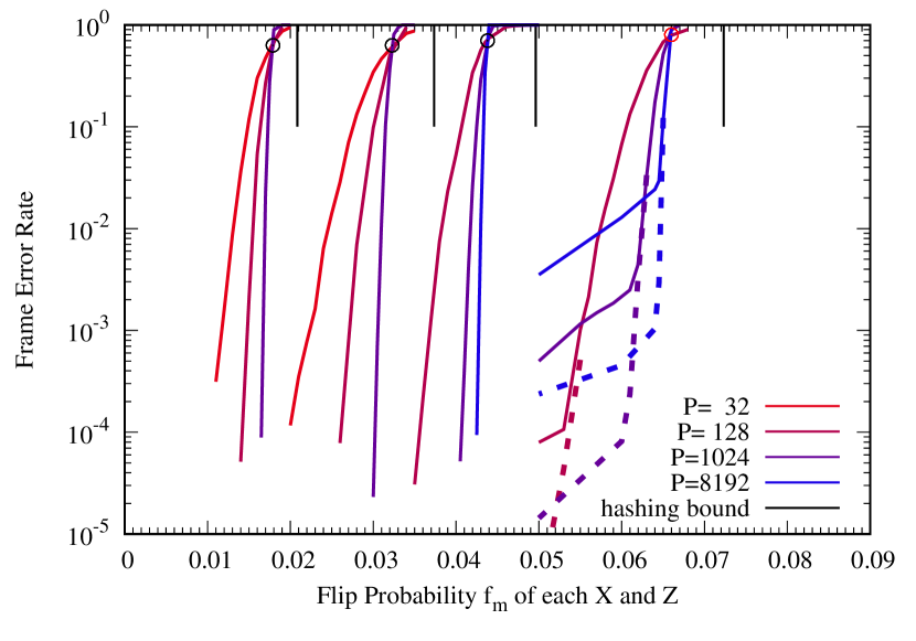
Figure 1: Decoding performance $(f_{m},\mathrm{FER})$ of the proposed method (dashed).

IX Conclusion and Future Work

In this paper, we proposed an efficient method for correcting estimation errors in quantum LDPC codes. Our method demonstrates significant improvement in decoding performance, particularly in reducing the error floor, which has been a key challenge in previous approaches.

Despite the improvements, certain errors, particularly those resulting from Type-III estimation errors, remain an inherent challenge. These errors are specific to the code structure and cannot be easily addressed without revisiting the code construction process. However, eliminating such errors would pave the way for achieving even deeper error floors, which would further enhance the practical performance of quantum error correction.

References

- [1] D. Bluvstein, S. J. Evered, A. A. Geim, S. H. Li, H. Zhou, T. Manovitz, S. Ebadi, M. Cain, M. Kalinowski, D. Hangleiter, et al., “Logical quantum processor based on reconfigurable atom arrays,” Nature, vol. 626, no. 7997, pp. 58–65, 2024.
- [2] J. Preskill, “Quantum computing in the NISQ era and beyond,” Quantum, vol. 2, p. 79, 2018.
- [3] D. Komoto and K. Kasai, “Quantum error correction near the coding theoretical bound,” arXiv preprint arXiv:2412.21171, 2024.
- [4] K. Kasai, M. Hagiwara, H. Imai, and K. Sakaniwa, “Quantum error correction beyond the bounded distance decoding limit,” IEEE Trans. Inf. Theory, vol. 58, no. 2, pp. 1223–1230, 2012.
- [5] D. Gottesman, “Stabilizer codes and quantum error correction,” Ph.D. dissertation, California Institute of Technology, May 1997.
- [6] A. R. Calderbank and P. W. Shor, “Good quantum error-correcting codes exist,” Phys. Rev. A, vol. 54, no. 2, pp. 1098–1105, Aug. 1996.
- [7] A. M. Steane, “Multiple particle interference and quantum error correction,” vol. 452, no. 1954, pp. 2551–2577, 1996.
- [8] T. Nozaki, K. Kasai, and K. Sakaniwa, “Error floors of non-binary LDPC codes,” in 2010 IEEE International Symposium on Information Theory, 2010, pp. 729–733.