The simplest 2D quantum walk detects chaoticity

Abstract

Quantum walks have been actively studied from many perspectives, mainly from the statistical physics and quantum information points of view. We here determine the influence of basic chaotic features on the walker behavior. We consider an extremely simple model consisting of alternate one-dimensional walks along the two spatial coordinates of bidimensional closed domains (hard wall billiards). The chaotic or regular behavior that the shape of the boundary induces in the deterministic classical equations of motion and that translates into chaotic signatures for the quantized problem also results in sharp differences for the spectral statistics and morphology of the eigenfunctions of the quantum walker. Unexpectedly, two different quantum mechanical problems share the same kind of features related to the corresponding classical dynamics of one of them.

I Introduction

Quantum Walks (QWs), originally proposed by Aharonov [1], have become an important and very active area of physics. This interest comes from their efficient way of capturing diffusive properties, which in turn provided many applications in quantum information [2, 3, 4] and quantum optics [5, 6]. In particular, they are suitable to explain and build search algorithms [7], like for example in 2D grids [8]. Moreover, they have been implemented in several experiments [9, 10, 11]. In their simplest form, QWs are quantum counterparts of the well-known classical problem of the random walker on the line, which takes a step to the right or left depending on the outcome of a coin toss. The straightforward quantum-mechanical counterpart can be thought of as a spin particle that moves to the right or left. This displacement depends on the spin state whose evolution is given by the so-called quantum coin, the analogue of the classical coin toss.

Given the relevance of QWs in finite systems applications, studying the effects of boundaries is of the utmost importance [12, 13]. Also, it is interesting to investigate their behavior with respect to the complexity of the landscape in which the walker is moving. For instance, could a minimal QW model reveal quantum signatures of chaos in the same way as the quantized models directly derived from the Hamilton’s classical equations of motion do? Considering the different nature of the dynamics involved, this is a challenging question that we want to address in this work. In fact, QWs are not direct quantizations, in the usual sense, of deterministic classical models.

In this respect, the quantum chaos arena [14] is where the signatures of classical chaos in the quantum realm have been traditionally studied. This area of physics provided many important findings, one of the most celebrated results being the so-called Bohigas-Giannoni-Schmit (BGS) [15] conjecture, which has so far been thoroughly tested. It prescribes a random matrix behavior for quantized chaotic Hamiltonian systems. Notably, this subject has become very active today. In particular, the well known level repulsion derived from BGS, generalized to open systems under the name of the Grobe-Haake-Sommers (GHS) conjecture [16], has been recently challenged in [17]. Another well studied phenomenon like the localization on marginally stable orbits of elsewhere chaotic systems – for example on bouncing ball trajectories – constitute a hallmark of quantum chaos.

Hence, our main point here is to borrow some concepts and tools from quantum chaos in order to discover the consequences that a dynamically chaotic domain has on QWs. For that purpose, we consider a very simple model consisting of a 2D QW constrained by a hard wall. A deterministic classical free particle moving inside will show regular or chaotic dynamics depending on the domain shape. We take the rectangle and the paradigmatic Bunimovich stadium billiards as examples of both behaviors, respectively. We conclude that a streamlined QW model consisting only of a single spin and alternate and independent movements along each coordinate perceives the different nature that these boundaries have at the classical level. This is reflected in the spectral behavior and also by the contrasting shapes of the position probability distributions corresponding to the eigenfunctions of the unitary evolution operator.

This paper is organized as follows: in Sec. II we describe our QW model, in Sec. III we show the results where we focus on the spectral behavior and the morphology of the spatial part of the eigenfunctions of the evolution operator. Finally, in Sec. IV we present our conclusions and outline some possible future developments.

II QW model

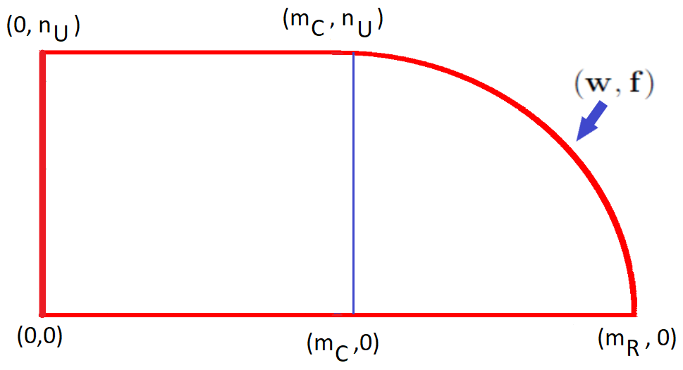
Figure 1: (Color online) Desymmetrized Bunimovich stadium billiard. Some integers $(m,n)$ specifying the particle position in a grid inside the billiard, and the shape functions used in the evolution operator are shown for reference. See Sec. II for details.

Our QW model is defined as a spin $1/2$ particle moving inside a 2D billiard, whose state at any (discrete) time is

$$|\Psi(t)\rangle=\sum_{m,n}U_{m}^{n}(t)\,|m,n,u\rangle+D_{m}^{n}(t)\,|m,n,d\rangle,$$ (1)

where $U_{m}^{n}$ and $D_{m}^{n}$ represent the probability amplitudes of the particle located at position $(m,n)$, with $(m,n)$ integers defining the position in a grid inside the billiard. Such particle can have either spin up, $u$ or spin down, $d$. The evolution is given by unitary operators that act on the spin space (the coin operator reflecting the coin toss) and on the position space (the walk operator reflecting the step taken by the walker conditional on the spin state). Additionally, there is a spin flip each time the walker reaches the border of the billiard. As an explicit motivation for this model, we can view the previous evolution as that corresponding to the motion of an electron inside a cavity. We can think of this model as consisting of two independent QWs, except for the fact that both share the same spin. The unbounded version is usually called Alternate QW (AQW) [18, 19].

Our bounded model in a rectangular billiard is implemented in the following way. We initially apply a SU(2) coin operator of the form

$$\hat{C}_{1}=\left(\begin{matrix}\cos{\alpha}&\sin{\alpha}\\ -\sin{\alpha}&\cos{\alpha}\end{matrix}\right),$$ (2)

acting on the spin space. Then, we proceed with a vertical displacement operator (acting solely in that direction) given by

$$\hat{W_{n}} = \sum_{0}^{n_{U}-1}|n+1\rangle\langle n|\otimes|U\rangle\langle U|$$ (3)

$$+ \sum_{1}^{n_{U}}|n-1\rangle\langle n|\otimes|D\rangle\langle D|+|0,U\rangle\langle 0,D|$$

$$+ |n_{U},D\rangle\langle n_{U},U|.$$

The last two terms in this expression correspond to the reflection at the boundary (i.e. at $0$ and $n_{U}$) by means of a spin flip (see a proof of its unitarity in the Appendix). Next, a second coin operator

$$\hat{C}_{2}=\begin{pmatrix}\cos{\beta}&\sin{\beta}\\ -\sin{\beta}&\cos{\beta}\end{pmatrix}$$ (4)

is applied. Finally, the horizontal displacement with reflections at $0$ and $m_{R}$ (again, acting only on the corresponding direction) is given by

$$\hat{W_{m}} = \sum_{0}^{m_{R}-1}|m+1\rangle\langle m|\otimes|U\rangle\langle U|$$ (5)

$$+ \sum_{1}^{m_{R}}|m-1\rangle\langle m|\otimes|D\rangle\langle D|+|0,U\rangle\langle 0,D|$$

$$+ |m_{R},D\rangle\langle m_{R},U|.$$

This completes the definition of our evolution operator for one time step.

For the Bunimovich stadium case, we just consider the upper right quarter of the billiard in order to avoid unwanted spatial symmetries. The boundary is introduced by modifying Eqs. (3) and (5) as follows

$$\hat{W_{n}} = \sum_{0}^{f(m)-1}|n+1\rangle\langle n|\otimes|U\rangle\langle U|$$ (6)

$$+ \sum_{1}^{f(m)}|n-1\rangle\langle n|\otimes|D\rangle\langle D|+|0,U\rangle\langle 0,D|$$

$$+ |f(m),D\rangle\langle f(m),U|$$

$$\hat{W_{m}} = \sum_{0}^{w(n)-1}|m+1\rangle\langle m|\otimes|U\rangle\langle U|$$ (7)

$$+ \sum_{1}^{w(n)}|m-1\rangle\langle m|\otimes|D\rangle\langle D|+|0,U\rangle\langle 0,D|$$

$$+ |w(n),D\rangle\langle w(n),U|$$

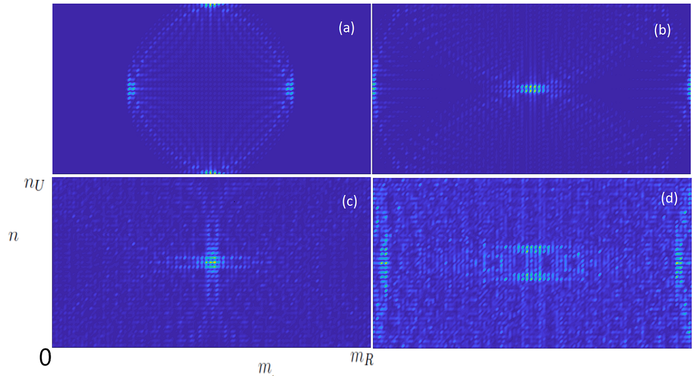
Figure 2: (Color online) Time evolution of a centered Gaussian distribution (see main text for details) at t = 38 (a), 76 (b), 152 (c), 232 (d), for the rectangular billiard. A $(m_{R},n_{U})=(150,75)$ position grid, and $\alpha=\beta=\pi/4$ have been used in the calculations.

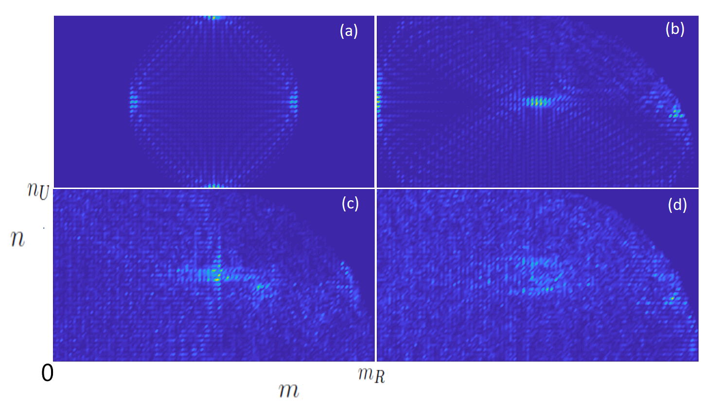
Figure 3: (Color online) Same as Fig. 2 for the Bunimovich stadium billiard.

Two shape functions, $f(m)$ and $w(n)$, have been introduced in the two previous expressions. Function $f(m)$, which corresponds to the maximum $n$ at each $m$, is given by

$$f(m)=\left\{\begin{array}[]{ll}n_{U}\hskip 81.09052pt\text{if}\;m\leq m_{C}\\ \sqrt{n_{U}^{2}-(m-m_{C})^{2}}\quad\text{if}\;m_{C}\leq m<m_{R}=2m_{C}.\end{array}\right.$$ (8)

Here, $m_{C}$ is the value $m$ at which the circular part of the boundary begins, while the lower limit is given by $0$, as in the rectangular billiard. Similarly, function $w(n)$ is the right limit of the displacement

$$w(n)=m_{C}+\sqrt{n_{U}^{2}-n^{2}}\quad\forall\ n,$$ (9)

with $0$ being the leftmost value, as before. See an illustration in Fig. 1. For comparison purposes, the rectangular billiard is taken as the rectangle in which the Bunimovich stadium is contained, both having a horizontal length two times the vertical one. Remind that the classical dynamics in the rectangular domain is regular.

In Fig. 2 we show some examples of the probability distribution at different times in the rectangular billiard case. We have taken a grid of size $m_{R}=150$ and $n_{U}=75$ and a normalized spatial Gaussian initial distribution located at the center of this domain, with amplitudes proportional to $\exp{(-(m-75)^{2}-(n-38)^{2})}$ with $73\leq m\leq 77$ and $36\leq n\leq 40$ and zero elsewhere; for spin up the amplitude is $1/\sqrt{2}$ and for spin down is $i/\sqrt{2}$. We have selected four evolution times that approximately correspond to a meaningful part of the evolved probability being reflected by the wall. In Fig. 3 we do the same as in the previous case, but now considering the Bunimovich stadium. It is clear that before the bounce on the circular part of the Bunimovich stadium both probability distributions coincide (a slight difference can be seen at $(m_{C},n_{U})$), as expected. But after the main reflection on the circle at $t=76$ they become markedly different, already showing regularity and strong symmetry in the rectangular billiard and the lack of them in the stadium. In fact, the probability peak at the center of the rectangular domain is gradually destroyed in the Bunimovich case for later times as can be checked by comparing the lower panels of both Figures.

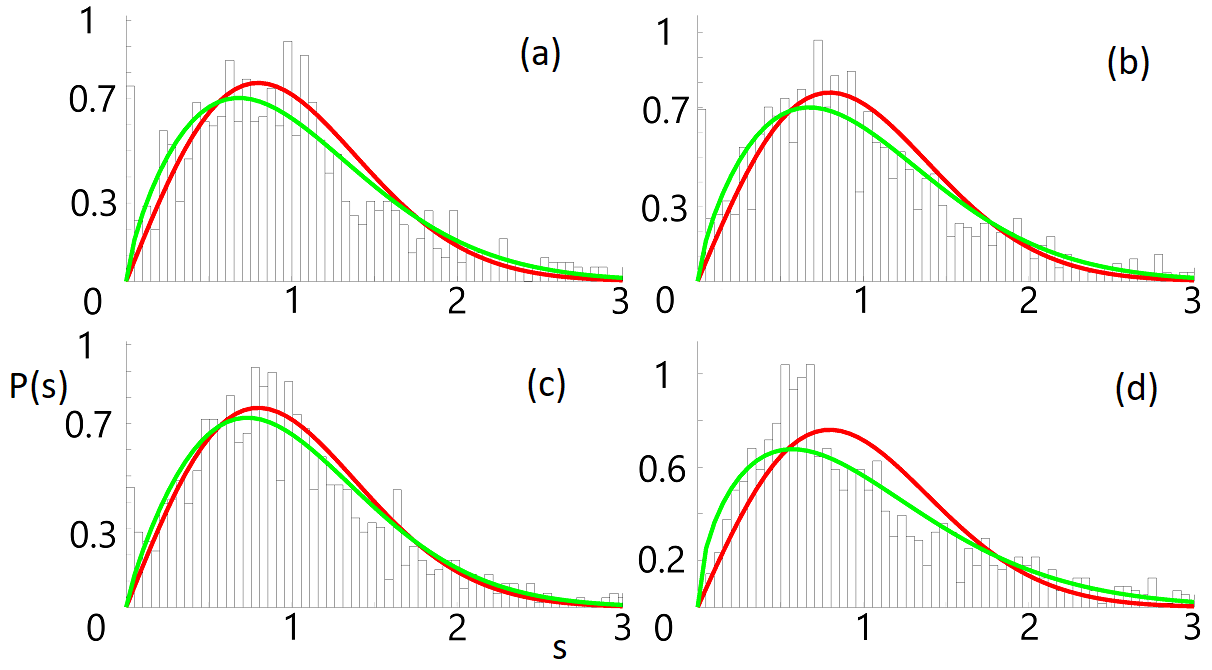
Figure 4: (Color online) Unfolded level spacing distributions $P(s)$ vs. $s$ for the Bunimovich stadium billiard with the following coin angles: $\alpha=\beta=\pi/8$ (a), $\alpha=\beta=\pi/7$ (b), $\alpha=\pi/8$ $\beta=\pi/9$ (c), and $\alpha=\pi/4$ $\beta=\pi/6$ (d). $P_{\rm W}$ and best fitting $P_{\rm B}$ (with the parameters and errors reported in Table 1) distributions, see Eqs. (10) and (12), are shown as red (gray) and green (light gray) solid lines, respectively.

III Chaotic signatures: spectral behavior and morphology of the eigenfunctions

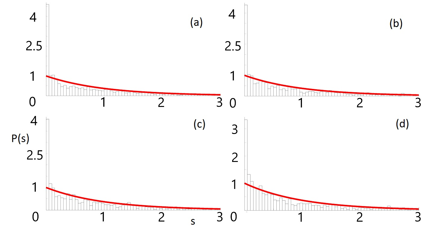
Figure 5: (Color online) Unfolded level spacing distributions $P(s)$ vs. $s$ for the rectangular billiard with the following coin angles: $\alpha=\beta=\pi/8$ (a), $\alpha=\beta=\pi/7$ (b), $\alpha=\pi/8$ $\beta=\pi/9$ (c), and $\alpha=\pi/4$ $\beta=\pi/6$ (d). $P_{\rm P}$ distribution (errors reported in Table 2) , see Eq. (11), is shown by means of red (gray) solid lines.

An unbounded one-dimensional QW is translationally invariant and as a consequence a simple Dispersion Relation (DR) can be obtained. A similar situation arises for the unbounded AQW in two dimensions [20], leading to a generalized DR which is a straightforward extension of the 1D solution. For a cylinder, a compact domain with periodic boundary conditions in one direction, the same effectively happens, and a DR has been derived for it [21]. On the other hand, general billiards consist of a completely bounded domain with reflective boundaries, which in the context of QWs we have implemented by means of spin flips.

III.1 Spectral statistics

Since in our case there is no analytical DR we proceed, in what follows, with numerical explorations of the behavior of our system by means of the spectral statistics and the morphology of the corresponding eigenfunctions.

We directly diagonalize the evolution operator for one time step, i.e. $\hat{W_{m}}\hat{C}_{2}\hat{W_{n}}\hat{C}_{1}$, in the spin-position basis, and study its (unfolded) spectrum for both the Bunimovich and rectangular stadium billiards. To speed up the computations, we take here a grid of size $(m_{R},n_{U})=(50,25)$ (notice that this grid defines a smaller position basis for the Bunimovich stadium case). It is also important to underline that desymmetrizing the Bunimovich stadium is a customary procedure in order to avoid unwanted symmetries, and then reveal the Wigner surmise (or other statistics in different systems) for the eigenvalues associated to the corresponding Hamiltonian. Failing to do so would allow the overlapping of uncorrelated spectra corresponding to different symmetry classes. Keeping our line of reasoning, we proceed in this way.

In Fig. 4 we show the spectral statistics, where the eigenphases (i.e. the phases of the complex unimodular eigenvalues) of the evolution operator have been considered to construct the histograms $P(s)$ of the unfolded level spacings $s$. After ordering the eigenphases between $0$ and $2\pi$, the unfolding is performed by simply dividing the distances between nearest neighbors by the mean (arithmetic) distance. In the different panels, we show the results for four different pairs of $\alpha$ and $\beta$ values; in Figs. 4(a) and (b) they are equal (symmetrical coins), while in (c) and (d) they are different (asymmetrical coins, see caption for details). Together with the histograms, we plot the Wigner surmise [22] as the red (gray) solid lines given by

$$P_{{\rm W}}(s)=\frac{\pi}{2}\ s\ \exp{\left(\frac{-\pi\ s^{2}}{4}\right)},$$ (10)

which describes the spectral behavior of chaotic Hamiltonian evolution and in principle is not directly applicable to our QW scenario. In the other end of level statistics, for regular systems the spectral spacings satisfy the Poisson distribution given by

$$P_{{\rm P}}(s)=\exp{(-s)}.$$ (11)

Given that the QW dynamics is different from the one corresponding to the quantum Hamiltonian of a free particle inside a billiard, deviations from $P_{{\rm W}}(s)$ could be expected. Hence, we have also fitted the data (minimizing the root mean square error) with a very simple function that interpolates between Poisson and the Wigner surmise, the Brody distribution [23], whose expression is

$$P_{{\rm B}}(s)=a\ s^{\delta}\ \exp{(-b\ s^{\delta+1})},$$ (12)

where $a=(\delta+1)b$, $b={\Gamma((\delta+2)/(\delta+1))}^{\delta+1}$, and $\delta$ is a parameter. The corresponding results are displayed by means of green (light gray) solid lines in Fig. 4 and the fitting values are shown in Table 1. We notice a general behavior that approximately follows the Wigner surmise since the best fitting Brody curve is closer to it ($\delta\in 0.55\sim 0.83$ and the error slightly lower in general) than Poisson ($\delta=0$). It is interesting to see that, besides the deviations from the exact Wigner curve, in all situations selected but one there is a high bar corresponding to the smallest level spacings, which abruptly falls in the next bin. This does not happen for $\alpha=\pi/4$ and $\beta=\pi/6$ (Fig. 4(d)), where level repulsion is indeed present, but the Wigner surmise performs worse. Symmetries due to the coin operator shape could exist. These symmetries though, are not enough to significantly uncorrelate the spectrum and lead to Poisson statistics.

Table 1: Fitting results and spectral distributions errors for the QW in the Bunimovich stadium billiard

Coins			Error
$\alpha$	$\beta$	$\delta$	$P_{\rm B}$	$P_{\rm W}$
$\pi/8$	$\pi/8$	0.730	0.104	0.111
$\pi/7$	$\pi/7$	0.718	0.104	0.113
$\pi/8$	$\pi/9$	0.833	0.088	0.092
$\pi/4$	$\pi/6$	0.552	0.093	0.126

In the case of the rectangular billiard, whose associated Hamiltonian is regular, we have evaluated the error of the Poisson distribution (see Fig. 5 and Table 2).

Table 2: Poisson distribution errors for the QW in the rectangular billiard

Coins		Error
$\alpha$	$\beta$	$P_{\rm P}$	$P_{\rm P}^{\prime}$
$\pi/8$	$\pi/8$	0.113	0.038
$\pi/7$	$\pi/7$	0.106	0.037
$\pi/8$	$\pi/9$	0.113	0.045
$\pi/4$	$\pi/6$	0.152	0.079

It becomes clear that the behavior is not strictly Poissonian, but it closely resembles it. In particular, when not considering the first and very large bars of the histograms the error of the Poisson distribution (we call it $P_{{\rm P}}^{\prime}$ in Table 2) is much lower. Hence, though the QW dynamics is clearly different from that of a quantum free particle moving inside a hard wall billiard, the statistical behavior of the spectra in these two cases is similar and allows to distinguish between them. Can we also identify other coincidences of this kind at the eigenfunction level?

III.2 Eigenfunctions morphology

To answer this we turn to analyze the morphology of the eigenfunctions. For that purpose we use the Participation Ratio (PR), a commonly used measure of localization in quantum chaos. The PR is calculated by first normalizing the eigenfunctions $|\Phi\rangle$ and then evaluating ${\rm PR}=(\sum_{m,n}|{U_{\Phi}}_{m}^{n}|^{4}+|{D_{\Phi}}_{m}^{n}|^{4})^{-1}$ (${U_{\Phi}}_{m}^{n}$ and ${D_{\Phi}}_{m}^{n}$ are the components of $|\Phi\rangle$). For example, in the rectangle the values of the PR range from $1$ to $2m_{R}n_{U}$ ($2\times 50\times 25$), roughly indicating how many position basis elements participate into a given eigenfunction (besides the factor $2$ coming from the spin part of the Hilbert space). As a consequence, larger PR values mean less localized states in this basis. In Fig. 6 we show the histogram corresponding to $P(\rm{PR})$ vs. PR.

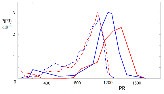
Figure 6: (Color online) $P(\rm{PR})$ vs. PR for both the Bunimovich stadium and the rectangular billiards. Dashed lines stand for the Bunimovich stadium histogram and solid ones for the rectangle case. Blue (black) lines correspond to $\alpha=\pi\ /4$ and $\beta=\pi\ /3$, while red (gray) lines to $\alpha=\beta=\pi\ /4$.

It can be directly observed that localization on around $1000$ basis elements is the approximate typical behavior for the Bunimovich stadium while on around $1250$ and $1400$ for the rectangle, which is only in part due to the different effective dimensions of the position basis in the two cases. This represents about half of the bases sizes (again, notice the spin space dimension). But not only the Bunimovich stadium billiard is more localized than the rectangle on average, the distribution is biased towards lower PR values in a meaningful way (PR approximately $\in[400,800]$). In what follows, by analyzing some representative cases we are going to deepen into this features.

We display some examples of eigenfunctions that help to understand the behavior of localization. In Fig. 7 we show two of the most delocalized and localized eigenfunctions of the Bunimovich stadium (upper row) and of the rectangular billiard (lower row), both for the symmetrical coins case. we notice that the delocalized states (left) are different with the Bunimovich’s one looking more irregular (or chaotic in the quantum chaos sense) and the rectangle’s one looking markedly more regular. For both maximally localized states the analogy with the Hamiltonian system becomes difficult and the different nature of the dynamics manifests itself. As a matter of fact, these extremely peaked eigenfunctions are not usually found in quantum billiards and deserve further study in the future.

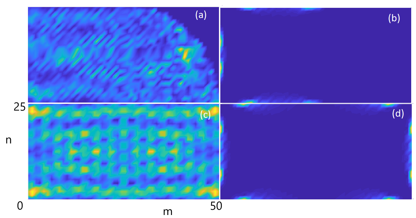
Figure 7: (Color online) Upper row: eigenfunctions of the Bunimovich stadium with PR=$1200.02$ (a) and PR=$57.13$ (b). Lower row: same for the rectangular billiard with PR=$1557.57$ (c) and PR=$104.01$ (d). In all cases $\alpha=\beta=\pi\ /4$.

We have also considered the case of asymmetrical coins in Fig. 8. In this case both systems apparently behave in an irregular fashion, but if one takes a closer look the only thing that changes from the previous Figure is the tilting provided by the asymmetrical coins (it amounts to biasing one of the 1D translations with respect to the other). Thus, the differences between regular and irregular behavior due to the shape of the boundaries in the corresponding Hamiltonian dynamics can still be detected.

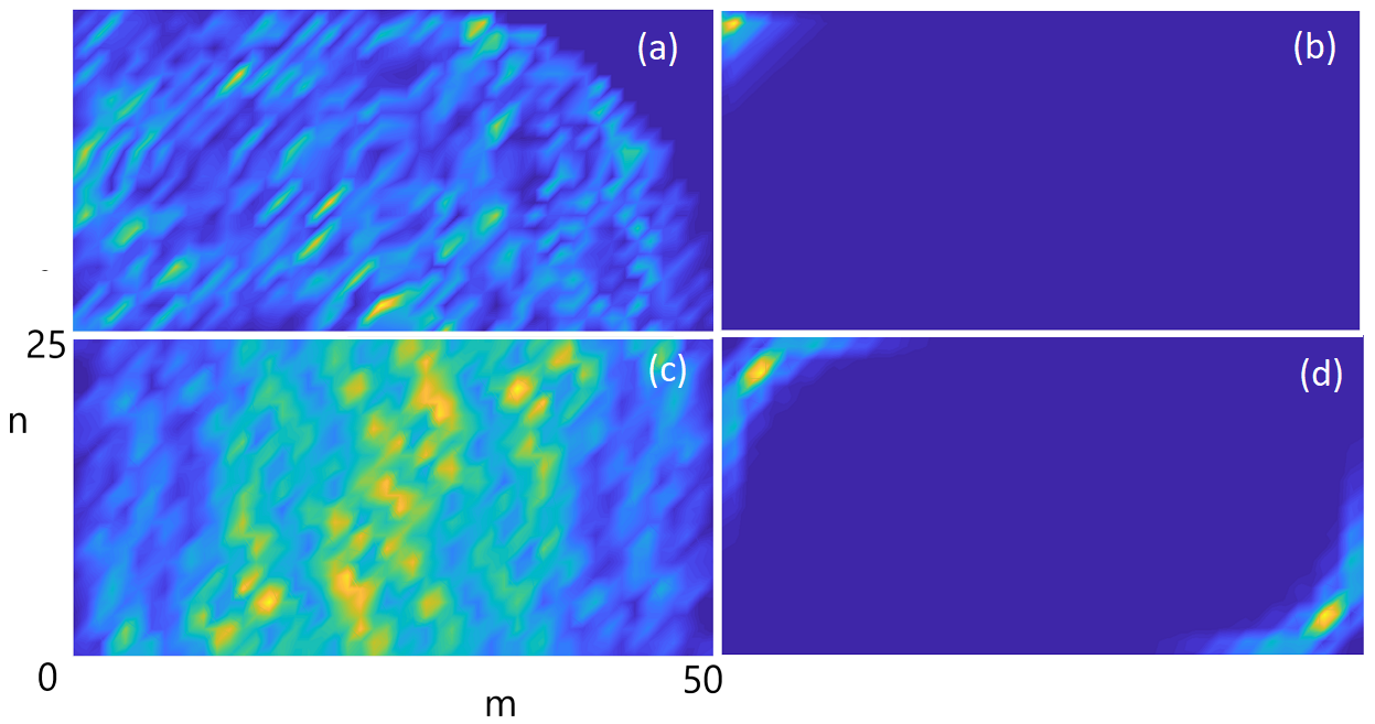
Figure 8: (Color online) Upper row: eigenfunctions of the Bunimovich stadium with PR=$1145.02$ (a) and PR=$36.41$ (b). Lower row: same for the rectangular billiard with PR=$1636.23$ (c) and PR=$148.11$ (d). In all cases $\alpha=\pi\ /4$ and $\beta=\pi\ /3$.

More interestingly, in the Bunimovich stadium billiard we have found localization on structures similar to those found in the corresponding Hamiltonian system, and which could be responsible for the greater localization found in this case (notice their typical PR values). In fact, there are bouncing ball states that closely resemble the ones ubiquitous in the quantum chaos literature [24, 25]. We show them by means of Fig. 9 for the symmetrical coins case and of Fig. 10 for the asymmetrical one. In the traditional quantum chaotic model, this family of eigenfunctions are localized on marginally stable orbits that form a continuous family. In the QW scenario this is remarkable, having in mind that we expect a purely diffusive behavior. Moreover, the typical sequence of horizontal excitations is also present in the QW and the only difference comes at the time of considering the asymmetrical coins which just tilt the bouncing balls.

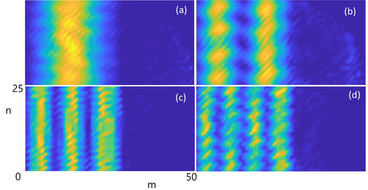
Figure 9: (Color online) Bouncing ball eigenfunctions of the Bunimovich stadium. Upper row: PR=$684.98$ (a) and PR=$797.18$ (b). Lower row: PR=$679.09$ (c) and PR=$780.15$ (d). In all cases $\alpha=\beta=\pi\ /4$.

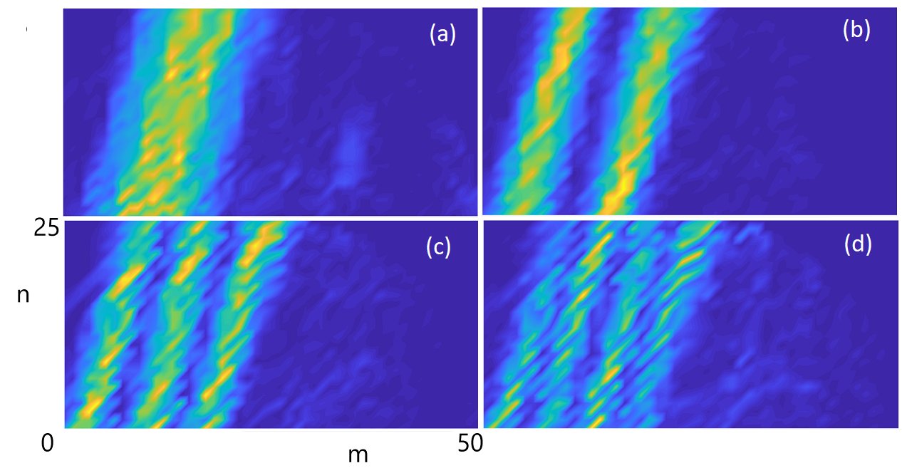
Figure 10: (Color online) Bouncing ball eigenfunctions of the Bunimovich stadium. Upper row: PR=$574.42$ (a) and PR=$594.73$ (b). Lower row: PR=$715.89$ (c) and PR=$678.73$ (d). In all cases $\alpha=\pi\ /4$ and $\beta=\pi\ /3$.

IV Conclusions

We have studied the properties of a QW inside compact bidimensional domains with different boundary shapes, characterized by a regular and irregular behavior of their corresponding classical and quantum Hamiltonian dynamics. The simple diffusive evolution given by the QW is able to detect these two regimes which in principle have only been associated to the classical behavior of a free particle inside these cavities and its corresponding quantization. This allows us to conclude that the simplest generalization of the QW on the line to 2D billiards constitutes a new paradigmatic example of quantum chaos.

A deeper theoretical explanation of this behavior is a promising avenue of research. One of the most interesting questions arises from the fact that though bouncing ball states have been found, no evidence of whispering gallery ones were obtained. This naturally indicates that the different properties of diffusive systems like QWs come into play at the time to detect chaoticity. The diffusion directions compared to the domain shape and symmetries are relevant, the details of their influence will be studied in the future. On the other hand, the underlying positions grid automatically associated with discrete QWs could induce different behaviors when compared to the usual billiard models. In fact, a hopping Hamiltonian on lattice billiards has been investigated in [26] showing the same spectral properties as the continuum counterparts, though in the open scenario new lattice scars were found. Is there something similar in the QWs case?

Also, we will consider more complex situations like having two particles inside the domain and other coins that would serve as different models for electrons inside a cavity [27]. Finally, we will investigate if our chaotic QW can improve 2D grid searches (as an alternative to the nonlinear QW model studied in [8], for instance).

Appendix A Unitarity of the evolution operator

It is worth showing the unitarity of the reflection mechanism at the billiard boundaries. Taking the most general vertical displacement:

$$\hat{W_{n}} = \sum_{0}^{f(m)-1}|n+1,U\rangle\langle n,U|$$ (13)

$$+ \sum_{1}^{f(m)}|n-1,D\rangle\langle n,D|+|0,U\rangle\langle 0,D|$$

$$+ |f(m),D\rangle\langle f(m),U|$$

and,

$$\hat{W}_{n}^{\dagger} = \sum_{0}^{f(m)-1}|n,U\rangle\langle n+1,U|$$ (14)

$$+ \sum_{1}^{f(m)}|n,D\rangle\langle n-1,D|+|0,D\rangle\langle 0,U|$$

$$+ |f(m),U\rangle\langle f(m),D|.$$

Hence,

$$\hat{W}_{n}^{\dagger}\hat{W}_{n} = \sum_{0}^{f(m)-1}|n,U\rangle\langle n,U|$$ (15)

$$+ \sum_{1}^{f(m)}|n,D\rangle\langle n,D|+|0,D\rangle\langle 0,D|$$

$$+ |f(m),U\rangle\langle f(m),U|,$$

or equivalently

$$\hat{W}_{n}^{\dagger}\hat{W}_{n} = \sum_{0}^{f(m)}|n,U\rangle\langle n,U|+\sum_{0}^{f(m)}|n,D\rangle\langle n,D|$$ (16)

$$= \sum_{0}^{f(m)}|n\rangle\langle n|\otimes(|U\rangle\langle U|+|D\rangle\langle D|)$$

which is the identity. The same happens for the most general horizontal displacement, completing the proof.

References

- [1] Y. Aharonov, L. Davidovich, and N. Zagury, Quantum random walks, Phys. Rev. A 48, 1687 (1993).
- [2] F. Nosrati et al., Quantum Information Spreading in a Disordered Quantum Walk, J. Opt. Soc. Am. B 38, 2570 (2021).
- [3] A. P. Hines and P. C. E. Stamp, Quantum walks, quantum gates, and quantum computers, Phys. Rev. A 75, 062321 (2007).
- [4] A. Ambianis, Quantum search algorithms, ACM SIGACT News 35, 22 (2004).
- [5] P. M. Preiss et al., Strongly correlated quantum walks in optical lattices, Science 347, 1229 (2015).
- [6] G. Maquiné Batalha, A. Volta, W.T. Strunz, and M. Galiceanu, Quantum transport on honeycomb networks, Sci. Rep. 12, 6896 (2022).
- [7] R. Portugal, Quantum walks and search algorithms (Springer Nature, Switzerland, 2018).
- [8] G. Di Molfetta and B. Herzog, Searching via nonlinear quantum walk on the 2D-grid, Algorithms 13, 305 (2020).
- [9] Hao Tang et al., Experimental twodimensional quantum walk on a photonic chip, Sci. Adv. 4, 3174 (2018).
- [10] Q.P. Su et al., Experimental demonstration of quantum walks with initial superposition states, npj Quantum Inf. 5, 40 (2019).
- [11] Z.Q. Jiao et al., Two-dimensional quantum walks of correlated photons, Optica 8, 1129 (2021).
- [12] J. Rodrigues, N. Paunkovic, and P. Mateus, A simulator for discrete quantum wals on lattices, Int. J. Mod. Phys. C 28, 1750055 (2017).
- [13] E. Bach, S. Coppersmith, M.P. Goldschen, R. Joynt, and J. Watrous, One dimensional Quantum Walks with absorbing boundaries, JCSS 69, 562 (2004).
- [14] F. Haake, Quantum Signatures of Chaos, Springer-Verlag, Berlin, (2004).
- [15] O. Bohigas, M.J. Giannoni, and C. Schmit, Characterization of chaotic quantum spectra and universality of level fluctuation laws, Phys. Rev. Lett. 52, 1 (1984).
- [16] R. Grobe and F. Haake, Universality of cubic level repulsion for dissipative quantum chaos, Phys. Rev. Lett. 62, 2893 (1989).
- [17] D. Villaseñor, L.F. Santos, and P. Barberis-Blostein, Breakdown of the quantum distinction of regular and chaotic classical dynamics in dissipative systems, Phys. Rev. Lett. 133, 240404 (2024).
- [18] C. Di Franco, M. Mc Gettrick, and Th. Busch, Mimicking the probability distribution of a two-dimensional Grover walk with a single-qubit coin, Phys. Rev. Lett. 106, 080502 (2011).
- [19] L.A. Bru, M. Hinarejos, F. Silva, G.J. de Valcárcel, and E Roldán, Electric quantum walks in two dimensions, Phys. Rev. A 93, 032333 (2016).
- [20] E. Roldán, C. Di Franco, F. Silva, and G.J. de Valcárcel, N-dimensional alternate coined quantum walks from a dispersion-relation perspective, Phys. Rev. A 87, 022336 (2013).
- [21] L.A. Bru, G.J. de Valcárcel, G. Di Molfetta, A. Pérez, E. Roldán, and F. Silva, Quantum walk on a cylinder, Phys. Rev. A 94, 032328 (2016).
- [22] M.L. Mehta, Random matrices, Academic Press, San Diego, (1991).
- [23] T. Prosen and M. Robnik, Energy level statistics in the transition region between integrability and chaos, J. Phys. A: Math. Gen. 26, 2371 (1993).
- [24] E.G. Vergini and G.G. Carlo, Semiclassical quantization with short periodic orbits, J. Phys. A: Math. Gen. 33, 4717 (2000).
- [25] S. Selinummi, J. Keski-Rahkonen, F. Chalangari, and E. Räsänen, Formation, prevalence, and stability of bouncing-ball quantum scars Phys. Rev. B 110, 235420 (2024).
- [26] V. Fernández-Hurtado, J. Mur-Petit, J.J. García-Ripoll and R.A. Molina, Lattice scars: surviving in an open discrete billiard, New J. Phys. 16, 035005 (2014).
- [27] A. Melnikov and L. Fedichkin, Quantum walks of interacting fermions on a cycle graph, Sci Rep 6, 34226 (2016).