Finite mixture representations of zero-&-$N$-inflated distributions for count-compositional data

Abstract

We provide novel probabilistic portrayals of two multivariate models designed to handle zero-inflation in count-compositional data. We develop a new unifying framework that represents both as finite mixture distributions. One of these distributions, based on Dirichlet-multinomial components, has been studied before, but has not yet been properly characterised as a sampling distribution of the counts. The other, based on multinomial components, is a new contribution. Using our finite mixture representations enables us to derive key statistical properties, including moments, marginal distributions, and special cases for both distributions. We develop enhanced Bayesian inference schemes with efficient Gibbs sampling updates, wherever possible, for parameters and auxiliary variables, demonstrating improvements over existing methods in the literature. We conduct simulation studies to evaluate the efficiency of the Bayesian inference procedures and to illustrate the practical utility of the proposed distributions.

[1]organization=Hamilton Institute and Department of Mathematics and Statistics, Maynooth University

[2]organization=School of Mathematics and Statistics, Insight Centre for Data Analytics, University College Dublin

1 Introduction

The excess of zeros in count-compositional data occurs when one or more categories have a larger number of observed zeros than expected under common statistical distributions, such as the multinomial and Dirichlet-multinomial. The primary complication in multivariate count-compositional settings, compared to univariate cases, is that the excess zeros can occur in a single category or across multiple categories. When zero-inflation occurs in all but one category, this gives rise to the related phenomenon of $N$-inflation.

We discuss two multivariate probability distributions designed to address the prevalence of excess zeros in count-compositional data. We introduce a unifying framework that represents these models as finite mixtures. Specifically, we derive a novel zero-&-$N$-inflated multinomial (ZANIM) distribution, which is based on multinomial mixture components, and extend this approach to the zero-&-$N$-inflated Dirichlet-multinomial (ZANIDM). Although ZANIDM was first introduced by Koslovsky [1], under the name ZIDM, it was described only through a stochastic representation via a mixture distribution on the count probabilities. We fully characterise ZANIDM as a sampling distribution on the counts capable of simultaneously modelling both zero-and-$N$-inflation and overdispersion using Dirichlet-multinomial mixture components.

Our paper is structured as follows. We derive the finite mixture representations of both distributions in Section 2. These representations facilitate the derivation of some key theoretical properties of the distributions in Section 3. We propose Bayesian frameworks for model inference in Section 4. In particular, for ZANIDM, we note that it is possible to improve the efficiency of the MCMC algorithm by marginalising out a latent variable, which was not done by Koslovsky [1]. We present two simulation studies in Section 5 which i) compare different MCMC algorithms for inferring the parameters of ZANIDM and ii) illustrate the practical utility of both distributions when dealing with zero-inflation in count-compositional data. We conclude with a brief discussion in Section 6. Additional details on associated derivations and inference schemes for both distributions are deferred to the Appendices. We also provide further results in the Supplementary Material. For now, we begin by describing some related proposals.

1.1 Related work

Many extensions of the multinomial distribution have been proposed in the literature, most of which aim to address extra variation relative to the its inherent limitations, particularly its negative covariance structure. Notable examples include the Dirichlet-multinomial [2], the finite mixture of multinomials [3], and the Conway-Maxwell-multinomial distribution [4, 5]. In contrast, there are relatively few extensions of the multinomial or other count-compositional distributions which address the issue of excess zeros. Key contributions in this area include the following: Diallo et al. [6], who studied a specific case of zero-inflation in the multinomial distribution; Tang and Chen [7], who introduced the zero-inflated generalised Dirichlet-multinomial by modifying the Beta stick-breaking representation of the generalised Dirichlet distribution [8] to incorporate a zero-augmented Beta distribution; and Tuyl [9], who proposed a spike-and-slab prior for the multinomial probability parameter, assigning a positive probability mass to zero.

More recently, Zeng et al. [10] proposed the zero-inflated logistic normal multinomial, while Koslovsky [1] introduced a zero-inflated extension of the Dirichlet-multinomial, leveraging its gamma representation to incorporate zero-inflation into the count probabilities. Notably, both of these recent works focus on modifying the latent space rather than the sampling distribution of the counts, and we note some similarities in their derivations. However, Zeng et al. [10] and Koslovsky [1] primarily focus on modelling data from human microbiome studies, without emphasising the theoretical properties of their models. Our paper addresses this gap by: (i) presenting a unified framework for both models, reformulating them in terms of their unconditional representation without latent variables, (ii) leveraging this framework to derive key statistical properties for both models, and (iii) discussing Bayesian inference using their latent structures while proposing improvements to the sampling scheme for the ZANIDM distribution.

2 Derivation of the distributions

In what follows, we shall assume that $\mathbf{Y}=(Y_{1},\ldots,Y_{d})$ denotes a $d$-dimensional random vector of count compositions, where $\mathbf{y}=(y_{1},\ldots,y_{d})$ represents the observed data.

2.1 Zero-&-$N$-inflated multinomial distribution

A well-known probability distribution for describing count-compositional data is the multinomial distribution, whose probability mass function (PMF) is given by

$$\Pr[\mathbf{Y}=\mathbf{y};\bm{\theta}]=\binom{N}{y_{1}\dots y_{d}}\,\prod_{j=1}^{d}\theta_{j}^{y_{j}},\quad\mathrm{for}\quad\mathbf{y}\in\Omega_{d,N},$$ (1)

where $\bm{\Omega}_{d,N}=\left\{\mathbf{y}\in(0,1,\ldots,N)^{d};\sum_{j=1}^{d}\,y_{j}=N\right\}$ is the sample space, represented by a discrete simplex space $\bm{\theta}=(\theta_{1},\ldots,\theta_{d})$, with $\theta_{j}\geq 0$ denoting the probability of occurrence of category $j$, subject to the constraint $\sum_{j=1}^{d}\,\theta_{j}=1$. Here, $N$ is a known constant denoting the number of trials. Within this paradigm, we shall consider the parameterisation $\theta_{j}=\lambda_{j}/\sum_{k=1}^{d}\lambda_{k},$ where $\lambda_{j}$ is a measure of the relative importance of category $j$; when it is normalised, it gives the probability of category $j$, i.e., $\theta_{j}$.

A well-known data-augmentation (see, e.g., [11]), which leads to conditional independence for the category-specific multinomial parameters, uses the latent variable

$$(\phi\mid\bm{\lambda},\mathbf{y})\sim\operatorname{Gamma}\left[N,\sum_{j=1}^{d}\,\lambda_{j}\right],$$ (2)

which yields the following joint PMF for $\mathbf{Y}$ and $\phi$:

$$\Pr[\mathbf{Y}=\mathbf{y},\phi;\bm{\lambda}]=\dfrac{N!\,\phi^{N-1}}{\Gamma(N)}\,\prod_{j=1}^{d}\left[\dfrac{\lambda_{j}^{y_{j}}e^{-\lambda_{j}\,\phi}}{y_{j}!}\right],$$ (3)

where the marginal PMF of $\mathbf{y}$ follows that of Equation (1). Note that the augmented likelihood factors into independent terms for each $\lambda_{j}$. The same likelihood, up to a multiplicative constant, can be obtained via the Poisson-multinomial transformation of Baker [12]. For an arbitrary category $j$, the likelihood contribution of an observation takes a ‘Poisson-type’ form, i.e.,

$$p(y_{j},\phi\mid\lambda_{j})\propto\dfrac{\lambda_{j}^{y_{j}}\,e^{-\lambda_{j}\,\phi}}{y_{j}!},\quad y_{j}=0,1,2,\ldots,N.$$ (4)

The excess of zeros in multinomial count data may be structural in nature. A reasonable way to address this using the augmented likelihood given in Equation (3) is to introduce additional parameters to account for zero-inflation with respect to each category. Specifically, we can consider a mixture-type model by adjusting the ‘Poisson-type’ form in Equation (4) to include a zero-inflation parameter. Thus, the likelihood contribution for category $j$ adopts a ‘ZI-Poisson-type’ form, i.e.,

$$p(y_{j},\phi\mid\lambda_{j},\zeta_{j})\propto\zeta_{j}\,\mathds{1}_{0}\left(y_{j}\right)+\left(1-\zeta_{j}\right)\,\dfrac{\lambda_{j}^{y_{j}}\,e^{-\lambda_{j}\,\phi}}{y_{j}!},\,\quad y_{j}=0,1,2,\ldots,N,$$ (5)

where $\zeta_{j}\in[0,1]$ denotes the probability of zero-inflation of category $j$, which we henceforth refer to as the ‘excess of zero parameter’, and $\mathds{1}_{0}(y_{j})$ is the usual indicator function $\mathds{1}(y_{j}=0)$, which evaluates to $1$ if $y_{j}=0$ or $0$ otherwise. It is important to note that $Y_{j}$ may still be $0$ even if $\zeta_{j}=0$. We refer to such zeros as ‘sampling zeros’, in contrast to ‘structural zeros’.

By plugging Equation (5) into Equation (3), we have that

$$\Pr[\mathbf{Y}=\mathbf{y},\phi;\bm{\lambda},\bm{\zeta}]=\dfrac{N!\,\phi^{N-1}}{\Gamma(N)}\,\prod_{j=1}^{d}\left[\zeta_{j}\,\mathds{1}_{0}(y_{j})+(1-\zeta_{j})\,\dfrac{\lambda_{j}^{y_{j}}\,e^{-\lambda_{j}\,\phi}}{y_{j}!}\right].$$ (6)

We now aim to marginalise out the latent variable $\phi$ from Equation (6) and ensure that the function $\int\Pr[\mathbf{Y}=\mathbf{y},\phi;\bm{\lambda},\bm{\zeta}]\mathop{}\!\mathrm{d}\phi$ will be a proper PMF. We state our main result concerning the PMF of this new distribution, named the zero-&-$N$-inflated multinomial (ZANIM) distribution, after first introducing some notation that will help to represent ZANIM as a finite mixture.

Definition 2.1.

Let $\mathfrak{K}=\{\mathcal{K}\subseteq\{1,\ldots,d\};1\leq\lvert\mathcal{K}\rvert\leq d-2\}$ represent the set of all subsets $\mathcal{K}$ of $\{1,\ldots,d\}$ with cardinality between $1$ and $d-2$, such that the subsets $\mathcal{K}$ gather categories with counts of zero, excluding the cases where exactly $d$ and $d-1$ categories are zero-inflated.

Definition 2.2.

Let $\bm{\zeta}=(\zeta_{1},\ldots,\zeta_{d})$, with $\zeta_{j}\in[0,1]$, and let $\eta_{d}=\prod_{j=1}^{d}\,(1-\zeta_{j})$, $\eta_{0}=\prod_{j=1}^{d}\,\zeta_{j}$, and $\eta_{N}^{(j)}=(1-\zeta_{j})\,\prod_{k\colon k\neq j}\zeta_{k}$, for $j=1\ldots,d$. We define $\eta_{\mathcal{K}}=\prod_{k\in\mathcal{K}}\zeta_{k}\,\prod_{j\notin\mathcal{K}}(1-\zeta_{j})$ for each $\mathcal{K}\in\mathfrak{K}$ and let $\bm{\eta}_{\mathfrak{K}}=\{\eta_{\mathcal{K}};\mathcal{K}\in\mathfrak{K}\}$ denote the set of such terms. The full set of mixture weights $\bm{\eta}=\{\eta_{d},\eta_{0},\eta_{N}^{(1)},\ldots,\eta_{N}^{(d)},\bm{\eta}_{\mathfrak{K}}\}$ are functions of the $\bm{\zeta}$ parameters and sum to one as required.

Definition 2.3.

Let $\delta_{\mathbf{0}_{d}}(\cdot)=\prod_{j=1}^{d}\delta_{0}(\cdot)$, where $\delta_{x}(\cdot)$, is the Dirac measure which places a point mass at $x$. If a random variable follows $X\sim\delta_{x}(\cdot)$, then its distribution function is $F_{X}(a)=\Pr[X\leq a]=1$ if $a\geq x$ and $0$ otherwise.

Proposition 2.1.

The zero-&-$N$-inflated multinomial distribution, denoted by $\mathbf{Y}\sim\operatorname{ZANIM}_{d}[N,\bm{\theta},\bm{\zeta}]$, is a finite mixture distribution of $2^{d}$ components with PMF given by

$$\Pr[\mathbf{Y}=\mathbf{y};\bm{\theta},\bm{\zeta}] =\eta_{d}\,\binom{N}{y_{1}\dots y_{d}}\,\prod_{j=1}^{d}\theta_{j}^{y_{j}}$$ (7)

$$\phantom{=}~+\sum_{j=1}^{d}\,\eta_{N}^{(j)}\left[\mathds{1}_{0}\left(\sum_{k\colon k\neq j}y_{k}\right)\,\right]$$ (8)

$$\phantom{=}~+\sum_{\mathcal{K}\in\mathfrak{K}}\eta_{\mathcal{K}}\left[\mathds{1}_{0}\left(\sum_{k\in\mathcal{K}}y_{k}\right)\binom{N}{\{y_{j}\}_{j\notin\mathcal{K}}}\prod_{j\notin\mathcal{K}}\left(\theta_{j}^{\mathcal{K}}\right)^{y_{j}}\right]$$ (9)

$$\phantom{=}~+\eta_{0}\,\prod_{j=1}^{d}\,\mathds{1}_{0}(y_{j})\quad\mathrm{for}\quad\mathbf{y}\in\bm{\Omega}_{d,N}^{0},$$ (10)

where $\bm{\theta}=(\theta_{1},\ldots,\theta_{d})$, with $\theta_{j}\geq 0$ and $\sum_{j=1}^{d}\theta_{j}=1$, $\theta_{j}^{\mathcal{K}}=\theta_{j}/(1-\sum_{\ell\in\mathcal{K}}\,\theta_{\ell})$, and $\bm{\zeta}=(\zeta_{1},\ldots,\zeta_{d})$, with $\zeta_{j}\in[0,1]$. The mixture weights $\bm{\eta}$ are functions of $\bm{\zeta}$ (see Definition 2.2).

Proof.

See A for details. ∎

Remark 2.1.

In Proposition 2.1, $\bm{\Omega}_{d,N}^{0}=\bm{\Omega}_{d,N}\cup\mathbf{0}_{d}$ is an expansion of the multinomial support, which accounts for the case where $y_{j}=0\>\forall\>j=1,\ldots,d$. Although simultaneously observing zero counts for all categories may be a rarity in practice, the addition of the associated component in Equation (10) is necessary to ensure the validity of the PMF.

It is clear that ZANIM is a finite mixture of multinomials, along with two degenerate distributions for the cases where all counts are zero, corresponding to Equation (10), and where all but one category are zero, corresponding to Equation (8). Equation (7) is a multinomial with $d$ categories, $N$ trials, and probabilities $\bm{\theta}=(\theta_{1},\ldots,\theta_{d})$. Equation (9) represents multinomials with $N$ trials and probabilities $\theta_{j}^{\mathcal{K}}$ for all categories $j\notin\mathcal{K}$. We note, however, that a given $\mathbf{y}_{i}=\{y_{i1},\ldots,y_{id}\}$ can belong to as few as one and at most $2^{d-1}$ components, given the presence of indicator functions in the above PMF. Obviously, if there are no zeros in the given $\mathbf{y}_{i}$, then we just evaluate the purely multinomial component in Equation (7). In the special case where the entire $\mathbf{y}_{i}$ consists of zeros, we evaluate only the purely degenerate component in Equation (10). Otherwise, when $\mathbf{y}_{i}$ contains both zero and non-zero counts, we require the evaluation of $2^{q}$ components, where $q\in[1,d-1]$ denotes the number of observed zeros, including the purely multinomial component, the reduced multinomial components, and (when $q=d-1$ exactly) the corresponding $N$-inflated component. This simplifies the calculation of the likelihood by obviating the need to evaluate all $2^{d}$ components and highlighting how few components need to be evaluated when the number of zeros is low.

Proposition 2.2.

If $\mathbf{Y}\sim\operatorname{ZANIM}_{d}[N,\bm{\theta},\bm{\zeta}]$, then $\mathbf{Y}$ has the stochastic representation:

$$\mathbf{Y}\sim\eta_{0}\,\delta_{\mathbf{0}_{d}}(\cdot)+\sum_{j=1}^{d}\,\eta^{(j)}_{N}\,\mathbf{E}_{d}^{(j)}+\eta_{d}\,\operatorname{Multinomial}_{d}[N,\bm{\theta}]+\sum_{\mathcal{K}\in\mathfrak{K}}\,\eta_{\mathcal{K}}\,\operatorname{Multinomial}_{d}[N,\bm{\theta}_{0}^{\mathcal{K}}],$$ (11)

where $\mathbf{E}_{d}^{(j)}=(\delta_{N}(Y_{1}),\ldots,\delta_{0}(Y_{j-1}),\delta_{N}(Y_{j}),\delta_{0}(Y_{j+1}),\ldots,\delta_{0}(Y_{d}))$ denotes a vector of length $d$ with Dirac mass at $N$ in the $j$-th entry and Dirac masses at zero elsewhere, and $\bm{\theta}_{0}^{\mathcal{K}}$ reflects the fact that the entries of $\{\theta_{1}^{\mathcal{K}},\ldots,\theta_{d}^{\mathcal{K}}\}$ are zero for all $j\in\mathcal{K}$.

Proof.

Follows by identifying each mixture component in the PMF of ZANIM. ∎

Furthermore, we note that the mixture components in ZANIM are generated from a set of independent Bernoulli random variables, which leads to an alternative stochastic representation.

Proposition 2.3.

If $\mathbf{Y}\sim\operatorname{ZANIM}_{d}[N,\bm{\theta},\bm{\zeta}]$, then $\mathbf{Y}$ has the stochastic representation:

$$z_{j} \sim\operatorname{Bernoulli}[1-\zeta_{j}],\quad j=1,\ldots,d$$

$$(\mathbf{Y}\mid N,\bm{\theta},z_{1},\ldots,z_{d}) \sim\begin{cases}\delta_{\mathbf{0}_{d}}(\cdot)&\textrm{if}\>z_{j}=0\>\forall j\\ \operatorname{Multinomial}_{d}\left[N,z_{1}\dfrac{\theta_{1}}{1-s},\ldots,z_{d}\dfrac{\theta_{d}}{1-s}\right]&\textrm{otherwise},\end{cases}$$

where $s=\sum_{k=1}^{d}(1-z_{k})\theta_{k}$.

Proof.

Follows from the fact that the mixture weights defined in Definition 2.2 are products of Bernoulli probabilities. ∎

From the two stochastic representations above, we can easily generate values from ZANIM. Obviously, the representation in Proposition 2.3 is more efficient. We note that this representation has similarities to the zero-inflated logistic normal multinomial model of Zeng et al. [10]. However, in their model they do not consider the case where $z_{j}=0\>\forall\>j$, which has been studied in a specific space-time application by Douwes-Schultz et al. [13].

2.2 Zero-&-$N$-inflated Dirichlet-multinomial distribution

Leveraging the hierarchical representation of the Dirichlet-multinomial distribution (henceforth DM) through the compounding of the multinomial and Dirichlet distributions, Koslovsky [1] introduced the zero-inflated Dirichlet-multinomial model (ZIDM). We note that Koslovsky [1] provides a latent stochastic representation but not the marginal distribution. We now derive a probabilistic representation of this model. By later expressing ZIDM as a finite mixture, we conjecture that a more appropriate name would be the zero-&-$N$-inflated Dirichlet-multinomial (ZANIDM) distribution.

Definition 2.4.

A random vector $\mathbf{Y}$ is said to have a ZANIDM distribution if it has the following stochastic representation:

$$(\mathbf{Y}\mid\bm{\theta}) \sim\operatorname{Multinomial}[N,\theta_{1},\ldots,\theta_{d}]$$

$$(\lambda_{j}\mid z_{j},\alpha_{j}) \sim(1-z_{j})\,\delta_{0}(\cdot)+z_{j}\operatorname{Gamma}[\alpha_{j},1]$$

$$(z_{j}\mid\zeta_{j}) \sim\operatorname{Bernoulli}[1-\zeta_{j}],\quad j=1,\ldots,d,$$

where $\theta_{j}=\lambda_{j}/\sum_{k=1}^{d}\,\lambda_{k}$. In brief, $\mathbf{Y}\sim\operatorname{ZANIDM}_{d}[N,\bm{\alpha},\bm{\zeta}]$, where the parameters are: $N$, the number of trials, $\bm{\zeta}=(\zeta_{1},\ldots,\zeta_{d})$, s.t. $\zeta_{j}\in[0,1]$ is the excess of zero parameter of category $j$, and $\bm{\alpha}=(\alpha_{1},\ldots,\alpha_{d})$ are the concentration parameters with $\alpha_{j}>0$.

Proposition 2.4.

If $\mathbf{Y}\sim\operatorname{ZANIDM}_{d}[N,\bm{\alpha},\bm{\zeta}]$, then $\mathbf{Y}$ is a finite mixture of $2^{d}$ components with PMF given by

$$\Pr[\mathbf{Y}=\mathbf{y};\bm{\alpha},\bm{\zeta}] =\eta_{d}\,\dfrac{\Gamma(\alpha_{s})\,\Gamma(N+1)}{\Gamma(N+\alpha_{s})}\prod_{j=1}^{d}\,\left[\dfrac{\Gamma(y_{j}+\alpha_{j})}{\Gamma(\alpha_{j})\,\Gamma(y_{j}+1)}\right]$$ (12)

$$\phantom{=}~+\sum_{j=1}^{d}\,\eta_{N}^{(j)}\left[\mathds{1}_{0}\left(\sum_{k\colon k\neq j}y_{k}\right)\,\right]$$ (13)

$$\phantom{=}~+\sum_{\mathcal{K}\in\mathfrak{K}}\eta_{\mathcal{K}}\left[\mathds{1}_{0}\left(\sum_{i\in\mathcal{K}}y_{i}\right)\right]\dfrac{\Gamma(\alpha^{\mathcal{K}}_{s})\,\Gamma(N+1)}{\Gamma(N+\alpha^{\mathcal{K}}_{s})}\prod_{j\notin\mathcal{K}}\left[\dfrac{\Gamma(y_{j}+\alpha_{j})}{\Gamma(\alpha_{j})\,\Gamma(y_{j}+1)}\right]$$ (14)

$$\phantom{=}~+\eta_{0}\,\prod_{j=1}^{d}\,\mathds{1}_{0}(y_{j})\quad\mathrm{for}\quad\mathbf{y}\in\bm{\Omega}_{d,N}^{0},$$ (15)

where $\alpha_{s}=\sum_{j=1}^{d}\alpha_{j}$, $\alpha^{\mathcal{K}}_{s}=\sum_{j\notin\mathcal{K}}\,\alpha_{j}$, and the mixture weights $\bm{\eta}$ are as given in Definition 2.2.

Proof.

Marginalising out the latent variables $z_{j}$ and $\lambda_{j}$ in Definition 2.4 and accounting for the fact that $y_{j}=0$ when $\lambda_{j}=0\,(z_{j}=1)$ yields the desired result. See B for details. ∎

Recasting ZIDM as ZANIDM under our finite mixture model framework enables a fuller characterisation of the distribution which highlights, in particular, that the PMF also incorporates degenerate components to capture $N$-inflation. Notably, these components in Equation (13), as well as the case where $(y_{1}=\ldots=y_{d})=\mathbf{0}_{d}$ in Equation (15), are identical to their ZANIM counterparts in Equations (8) and (10), respectively. However, the remaining component distributions differ from ZANIM in that Equation (12) is a DM distribution and Equation (14) represents DM distributions of reduced dimension, in contrast to the multinomial distribution in Equation (7) and sets of reduced multinomial distributions in Equation (9) under ZANIM. Similarly, the finite mixture stochastic representation for ZANIDM is obtained by appropriately replacing the multinomial distributions in Proposition 2.2 with DM distributions.

Proposition 2.5.

If $\mathbf{Y}\sim\operatorname{ZANIDM}_{d}[N,\bm{\alpha},\bm{\zeta}]$, then $\mathbf{Y}$ has the stochastic representation:

$$\mathbf{Y}\sim\eta_{0}\,\delta_{\mathbf{0}_{d}}(\cdot)+\sum_{j=1}^{d}\,\eta^{(j)}_{N}\,\mathbf{E}_{d}^{(j)}+\eta_{d}\,\operatorname{DM}[N,\bm{\alpha}]+\sum_{\mathcal{K}\in\mathfrak{K}}\,\eta_{\mathcal{K}}\,\operatorname{DM}[N,\bm{\alpha}_{0}^{\mathcal{K}}],$$ (16)

where $\bm{\alpha}_{0}^{\mathcal{K}}$ has empty entries in $\bm{\alpha}$ for all $j\in\mathcal{K}$.

Proof.

Follows by identifying each mixture component in the PMF of ZANIDM. ∎

Remark 2.2.

Although ZANIM and ZANIDM have $2^{d}$ components, each distribution has only $2d$ parameters, since the component weights are functions of $\bm{\zeta}$ and the $\bm{\theta}$ and $\bm{\alpha}$ parameters fully determine the non-degenerate components under ZANIM and ZANIDM, respectively.

Remark 2.3.

The DM distribution arises from compounding the multinomial distribution with a probability vector which follows a Dirichlet distribution. The concentration of its random success probabilities around their mean is governed by $\alpha_{s}=\sum_{j=1}^{d}\alpha_{j}$. This variability diminishes as $\alpha_{s}\rightarrow\infty$ while keeping the proportions $\alpha_{j}/\alpha_{s}$ constant. Consequently, the Dirichlet distribution collapses to a degenerate distribution and the DM tends toward a multinomial distribution with fixed probabilities. Hence, we can relate the ZANIM and ZANIDM distributions by noting that, subject to keeping the corresponding parameters constant, the DM component in ZANIDM approaches a multinomial distribution with parameters $\alpha_{j}/\alpha_{s}$ as $\alpha_{s}\rightarrow\infty$, while the reduced DM components tend toward their multinomial counterparts with parameters $\alpha_{j}/\alpha_{s}^{\mathcal{K}}$ as $\alpha_{s}^{\mathcal{K}}\rightarrow\infty$. The remaining degenerate components are already common to both distributions.

3 Properties of ZANIM and ZANIDM

We outline some basic probabilistic properties of the ZANIM and ZANIDM distributions. Notably, the properties that follow are consequences of the fact that both the ZANIM and ZANIDM distributions can be seen as finite mixture distributions. As described in Propositions 2.1 and 2.4, both models have $K=2^{d}$ mixture components and the corresponding mixture weights $\bm{\eta}$ are functions of the excess of zero parameters $\bm{\zeta}$ (see Definition 2.2).

3.1 Marginal distribution of $Y_{j}$

When $\mathbf{Y}$ follows either the ZANIM or ZANIDM distribution, whose respective PMFs are given in Equations (7)–(10) and (12)–(15), the marginal PMF of the $j$-th element is itself a mixture. Under both distributions, obtaining the marginal PMF of $Y_{j}$ involves summing over the support of all other variables in $\mathbf{Y}$ while fixing $Y_{j}=k$. We use the well-known results that the multinomial and DM distributions have binomial and beta-binomial marginals, respectively, and introduce the following set notation to help write explicit formulas for the marginal PMFs.

Definition 3.1.

Let $\mathfrak{S}_{j}=\{\mathcal{S}_{j}\subseteq\{1,\ldots j-1,j+1\ldots,d\};1\leq\lvert\mathcal{S}_{j}\rvert\leq d-2\}$ represent the set of all subsets $\mathcal{S}_{j}$ of $\{1,\ldots,d\}\setminus\{j\}$ with cardinality between $1$ and $d-2$ for a given category $j$, such that the subsets $\mathcal{S}_{j}$ are obtained by excluding the cases which contain the $j$-th index from the subsets $\mathcal{K}$ described in Definition 2.1. Note that $\lvert\mathfrak{S}_{j}\rvert=2^{d-1}-2$.

Performing the required summation over each mixture component in the ZANIM and ZANIDM PMFs is reasonably straightforward. For ZANIM, the ‘non-zero’ component in Equation (7) and the ‘reduced dimension’ components in Equation (9) yield weighted binomial distributions, with weights given by $\eta_{d}$ and $\smash{\eta_{\mathcal{S}_{j}}=\prod_{k\in\mathcal{S}_{j}}\zeta_{k}\prod_{j\notin\mathcal{S}_{j}}(1-\zeta_{j})}$, respectively. The corresponding ZANIDM components in Equations (12) and (14), yield similarly weighted beta-binomial distributions. Recall that the remaining components are common to both distributions. Firstly, regarding the $N$-inflated components in Equations (8) and (13), we note that marginalising the $N$-inflation component corresponding to the $j$-th category contributes a degenerate mass at $N$ with probability $\smash{\eta_{N}^{(j)}}$, while the remaining $N$-inflated components each contribute a degenerate mass at $0$ with probability $\smash{\eta_{N}^{(k)}}$, for $k\neq j$. Secondly, the purely degenerate components in Equations (10) and (15) also contribute a degenerate mass at $0$ with probability $\eta_{0}$. Therefore, the marginal distribution of $Y_{j}$ is degenerate at $0$ with probability $\eta_{0}+\sum_{k\neq j}\eta_{N}^{(k)}$, which simplifies to $\zeta_{j}$. Finally, we obtain the marginal PMF of $Y_{j}$ under both distributions by combining the contributions of the associated marginal mixture components.

Proposition 3.1.

If $\mathbf{Y}\sim\operatorname{ZANIM}_{d}[N,\bm{\theta},\bm{\zeta}]$, then the marginal distribution of $Y_{j}$ is

$$\Pr[Y_{j}=k]=\begin{cases}\zeta_{j}+\eta_{d}\,\left(1-\theta_{j}\right)^{N}+\sum_{\mathcal{S}_{j}\,\in\,\mathfrak{S}_{j}}\,\eta_{\mathcal{S}_{j}}\,\big{(}1-\theta_{j}^{\mathcal{S}_{j}}\big{)}^{N}&\textrm{if}\quad k=0\\ \eta_{N}^{(j)}+\eta_{d}\,\theta_{j}^{N}+\sum_{\mathcal{S}_{j}\,\in\,\mathfrak{S}_{j}}\,\eta_{\mathcal{S}_{j}}\,\big{(}\theta_{j}^{\mathcal{S}_{j}}\big{)}^{N}&\textrm{if}\quad k=N\\ \eta_{d}\,p_{B}(k;N,\theta_{j})+\sum_{\mathcal{S}_{j}\,\in\,\mathfrak{S}_{j}}\,\eta_{\mathcal{S}_{j}}\,p_{B}\big{(}k;N,\theta_{j}^{\mathcal{S}_{j}}\big{)}&\textrm{if}\quad k=1,\,\ldots,N-1,\end{cases}$$

where $p_{B}(k;N,\theta)$ denotes the binomial PMF and $\theta_{j}^{\mathcal{S}_{j}}=\theta_{j}/(1-\sum_{\ell\in\mathcal{S}_{j}}\theta_{\ell})$.

Proof.

Follows directly from the concept of a marginal distribution, using Definition 3.1. ∎

Proposition 3.2.

If $\mathbf{Y}\sim\operatorname{ZANIDM}_{d}[N,\bm{\alpha},\bm{\zeta}]$, then the marginal distribution of $Y_{j}$ is

$$\Pr[Y_{j}=k]=\begin{cases}\zeta_{j}+\eta_{d}\,\dfrac{\operatorname{B}(\alpha_{j},N+\alpha^{(j)}_{s})}{\operatorname{B}(\alpha_{j},\alpha^{(j)}_{s})}+\sum_{\mathcal{S}_{j}\,\in\,\mathfrak{S}_{j}}\,\eta_{\mathcal{S}_{j}}\,\dfrac{\operatorname{B}(\alpha_{j},N+\alpha_{s}^{\mathcal{S}_{j}})}{\operatorname{B}(\alpha_{j},\alpha_{s}^{\mathcal{S}_{j}})}&\textrm{if}\quad k=0\\ \eta_{N}^{(j)}+\eta_{d}\,\dfrac{\operatorname{B}(\alpha_{j},N+\alpha^{(j)}_{s})}{\operatorname{B}(\alpha_{j},\alpha^{(j)}_{s})}+\sum_{\mathcal{S}_{j}\,\in\,\mathfrak{S}_{j}}\,\eta_{\mathcal{S}_{j}}\,\dfrac{\operatorname{B}(\alpha_{j}+N,\alpha_{s}^{\mathcal{S}_{j}})}{\operatorname{B}(\alpha_{j},\alpha_{s}^{\mathcal{S}_{j}})}&\textrm{if}\quad k=N\\ \eta_{d}\,p_{BB}\left(k;N,\alpha_{j},\alpha^{(j)}_{s}\right)+\sum_{\mathcal{S}_{j}\,\in\,\mathfrak{S}_{j}}\,\eta_{\mathcal{S}_{j}}\,p_{BB}\big{(}k;N,\alpha_{j},\alpha_{s}^{\mathcal{S}_{j}}\big{)}&\textrm{if}\quad k=1\,\ldots,N-1,\end{cases}$$

where $p_{BB}(k;N,\alpha_{j},\alpha^{(j)}_{s})$ denotes the beta-binomial PMF with $\alpha^{(j)}_{s}=\sum_{k\neq j}\alpha_{k}$, and $\operatorname{B}(a,b)=\Gamma(a)\Gamma(b)/\Gamma(a+b)$ is the Beta function. Similarly, $\smash{\alpha_{s}^{\mathcal{S}_{j}}=\sum_{k\notin\mathcal{S}_{j}}\alpha_{k}}$ where $k\notin\mathcal{S}_{j}$ implies the indices in $\{1,\ldots,d\}\setminus\{j\}$ that are not in $\mathcal{S}_{j}$.

Proof.

Follows directly from the concept of a marginal distribution, using Definition 3.1. ∎

Remark 3.1.

For the marginal probability distributions presented in Propositions 3.1 and 3.2, both $\Pr[Y_{j}=0]\rightarrow\zeta_{j}$ and $\Pr[Y_{j}=N]\rightarrow\eta_{N}^{(j)}$ as $N\rightarrow\infty$.

Remark 3.2.

From Propositions 3.1 and 3.2, the zero-&-$N$-inflated binomial and beta-binomial distributions are special cases of ZANIM and ZANIDM, respectively, when $d=2$.

From Propositions 3.1 and 3.2, we identify that the marginal distribution of $Y_{j}$ under ZANIM (or ZANIDM) is a finite mixture containing $2^{d-1}+1$ components. These mixture components are either degenerate at zero, degenerate at $N$, or follow binomial (or beta-binomial) distributions. Figure 1 shows some of the types of behaviour the marginal PMFs of ZANIM and ZANIDM can have in a three-dimensional setting, where the marginals of the random vector $\mathbf{Y}$ each have category-specific parameters. Each marginal distribution is specified such that the expectation is identical under both distributions (see Section 3.2 for details on their moments).

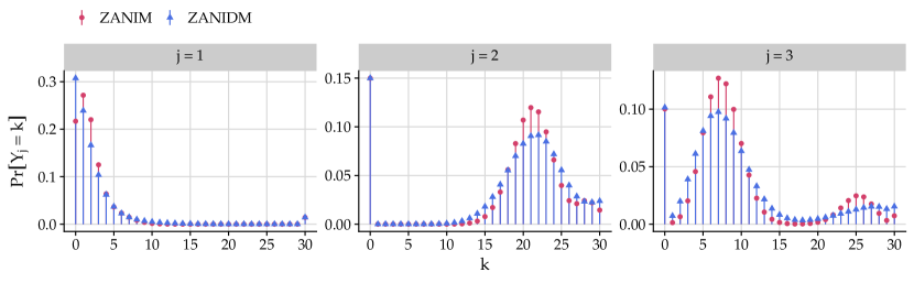
Figure 1: Marginal PMFs of ZANIM (red circles) and ZANIDM (blue triangles) with respective parameters $\bm{\theta}=(0.05,0.70,0.25)$ for ZANIM and $\bm{\alpha}=(2.0,28.0,10.0)$ for ZANIDM, along with $\bm{\zeta}=(0.05,0.15,0.10)$, and $N=30$ trials in each case.

The first marginal, $Y_{1}$, has a large spike at $k=0$ for both distributions, although this consists not only of structural zeros, but also many sampling zeros. This is understandable, given that the $\theta_{1}$ and $\alpha_{1}$ parameters take their lowest values among the three categories when $j=1$, and the zero-inflation parameter is also low $(\zeta_{1}=0.05)$. Although most of the probability mass is concentrated at lower values of $k$, there is also slight but nonetheless visible $N$-inflation at $k=N=30$, since the corresponding mixture weight, $\smash{\eta_{N}^{(1)}=(1-\zeta_{1})\,\zeta_{2}\,\zeta_{3}=0.00675}$, is non-zero. Interestingly, the ZANIDM marginal is more right-skewed and overdispersed than that of ZANIM, which also results in a larger spike at zero. The second marginal, $Y_{2}$, has a noticeable spike at $k=0$ also, given the higher $\zeta_{2}=0.15$, but peaks at higher $k$ values given that the $\theta_{2}$ and $\alpha_{2}$ parameters take their highest values among the three categories when $j=2$. As there is little mass assigned to values of $1\leq k<15$, this reflects a scenario where counts of zero reflect failure to detect a phenomenon which is more common. Finally, the nature of ZANIM as a finite mixture is most apparent for the third marginal, $Y_{3}$, given that both zero-inflation and moderate $N$-inflation are evident in addition to two other modes. Under ZANIM, the larger mode at $k=6$ is attributable to the purely multinomial component of the mixture, while the smaller mode at $k=24$ relates to the set of $\mathfrak{K}$ multinomial distributions of reduced dimension which capture ‘pairs of zero-inflation’ in the other categories. Regarding ZANIDM, we can clearly see a heavy right tail, which can be explained by the finite mixture components and the corresponding overdispersed nature of the beta-binomial distributions.

3.2 Moments

We briefly review a generic result that will be used for the derivations. Let $\bm{\tau}=\{\tau_{1},\ldots,\tau_{K}\}$ be a set of mixture weights, such that $\tau_{k}$ reflects a generic indexed mixture component without regard to whether that component relates to any particular case of zero-inflation, $N$-inflation, or otherwise. Let $W$ denote a discrete random variable indicating the mixture component, i.e., taking values in $\{1,\ldots,K\}$ with corresponding probabilities $\bm{\tau}$. Then, the expected value of $g(\mathbf{Y})$ can be expressed as $\mathbb{E}[g(\mathbf{Y})]=\sum_{k=1}^{K}\tau_{k}\,\mathbb{E}[g(\mathbf{Y})\mid W=k]$. Thus, since both distributions can be expressed as multivariate finite mixture distributions with $K=2^{d}$ components, we can easily obtain their moments. We recall that the component distributions are either degenerate random vectors (at $\delta_{\mathbf{0}_{d}}$ or $\mathbf{E}_{d}^{(j)}$), or multinomial/DM random vectors (including some of reduced dimension); see the stochastic representations in Equations (11) and (16).

Definition 3.2.

By analogy with the sets $\mathfrak{K}$ and $\mathfrak{S}_{j}$ described in Definitions 2.1 and 3.1, respectively, let $\mathfrak{R}_{jh}=\{\mathcal{R}_{jh}\subseteq\{1,\ldots,j-1,j+1,\ldots,h-1,h+1,\ldots,d\};1\leq\lvert\mathcal{R}_{jh}\rvert\leq d-2\}$ represent the set of all subsets $\mathcal{R}_{jh}$ of $\{1,\ldots,d\}\setminus\{j,h\}$ for a given pair of categories $j\neq h$.

Proposition 3.3.

Let $\mathbf{Y}\sim\operatorname{ZANIM}_{d}[N,\bm{\theta},\bm{\zeta}]$, then the mean and variance of the $j$-th entry of the random vector $\mathbf{Y}$, i.e., the random variable $Y_{j}$, are given by

$$\mathbb{E}[Y_{j}] =N\Big{(}\eta^{(j)}_{N}+\eta_{d}\,\theta_{j}+\sum_{\mathcal{S}_{j}\in\mathfrak{S}_{j}}\,\eta_{\mathcal{S}_{j}}\,\theta_{j}^{\mathcal{S}_{j}}\Big{)}$$

$$\operatorname{Var}[Y_{j}] =\eta_{N}^{(j)}\,N^{2}+\eta_{d}\,N\theta_{j}\left(1+\theta_{j}(N-1)\right)+\sum_{\mathcal{S}_{j}\in\mathfrak{S}_{j}}\,\eta_{\mathcal{S}_{j}}\,N\theta_{j}^{\mathcal{S}_{j}}\left(1+\theta_{j}^{\mathcal{S}_{j}}(N-1)\right)$$

$$\phantom{=}~-N^{2}\Big{(}\eta^{(j)}_{N}+\eta_{d}\,\theta_{j}+\sum_{\mathcal{S}_{j}\in\mathfrak{S}_{j}}\,\eta_{\mathcal{S}_{j}}\,\theta_{j}^{\mathcal{S}_{j}}\Big{)}^{2}.$$

The covariance between the random variables $(Y_{j},Y_{h})\>\forall\>j\neq h$ of the random vector $\mathbf{Y}$ is

$$\operatorname{Cov}[Y_{j},Y_{h}] =N(N-1)\,\Big{(}\eta_{d}\,\theta_{j}\,\theta_{h}+\sum_{\mathcal{R}_{jh}\in\,\mathfrak{R}_{jh}}\,\eta_{\mathcal{R}_{jh}}\,\theta_{j}^{\mathcal{R}_{jh}}\,\theta_{h}^{\mathcal{R}_{jh}}\Big{)}$$

$$\phantom{=}~-N^{2}\Big{(}\eta^{(j)}_{N}+\eta_{d}\,\theta_{j}+\sum_{\mathcal{S}_{j}\in\mathfrak{S}_{j}}\,\eta_{\mathcal{S}_{j}}\,\theta_{j}^{\mathcal{S}_{j}}\Big{)}\Big{(}\eta^{(h)}_{N}+\eta_{d}\,\theta_{h}+\sum_{\mathcal{S}_{h}\in\mathfrak{S}_{h}}\,\eta_{\mathcal{S}_{h}}\,\theta_{h}^{\mathcal{S}_{h}}\Big{)}.$$

Proof.

Follows from the moment properties of finite mixture distributions. ∎

Proposition 3.4.

Let $\mathbf{Y}\sim\operatorname{ZANIDM}_{d}[N,\bm{\alpha},\bm{\zeta}]$, then the mean and variance of the $j$-th entry of the random vector $\mathbf{Y}$, i.e., the random variable $Y_{j}$, are given by

$$\mathbb{E}[Y_{j}] =N\bigg{(}\eta^{(j)}_{N}+\eta_{d}\,\dfrac{\alpha_{j}}{\alpha_{s}}+\sum_{\mathcal{S}_{j}\in\mathfrak{S}_{j}}\,\eta_{\mathcal{S}_{j}}\,\dfrac{\alpha_{j}}{\alpha_{j}+\alpha_{s}^{\mathcal{S}_{j}}}\bigg{)}$$

$$\mathrm{Var}[Y_{j}] =\eta_{N}^{(j)}\,N^{2}+\eta_{d}\bigg{(}\dfrac{N\,\alpha_{j}[N(1+\alpha_{j})+\alpha_{s}^{(j)}]}{(\alpha_{j}+\alpha_{s}^{(j)})\,(1+\alpha_{j}+\alpha_{s}^{(j)})}\bigg{)}+\sum_{\mathcal{S}_{j}\in\mathfrak{S}_{j}}\,\eta_{\mathcal{S}_{j}}\,\bigg{(}\dfrac{N\,\alpha_{j}[N(1+\alpha_{j})+\alpha_{s}^{{\mathcal{S}_{j}}}]}{(\alpha_{j}+\alpha_{s}^{{\mathcal{S}_{j}}})\,(1+\alpha_{j}+\alpha_{s}^{{\mathcal{S}_{j}}})}\bigg{)}$$

$$\phantom{=}~-N^{2}\bigg{(}\eta^{(j)}_{N}+\eta_{d}\,\dfrac{\alpha_{j}}{\alpha_{s}}+\sum_{\mathcal{S}_{j}\in\mathfrak{S}_{j}}\,\eta_{\mathcal{S}_{j}}\,\dfrac{\alpha_{j}}{\alpha_{j}+\alpha_{s}^{\mathcal{S}_{j}}}\bigg{)}^{2}.$$

The covariance between the random variables $(Y_{j},Y_{h})\>\forall\>j\neq h$ of the random vector $\mathbf{Y}$ is

$$\operatorname{Cov}[Y_{j},Y_{h}] =N\eta_{d}\dfrac{\alpha_{j}\alpha_{h}}{\alpha_{s}}\bigg{[}N-\dfrac{N+\alpha_{s}}{1+\alpha_{s}}\bigg{]}$$

$$\phantom{=}~+N\sum_{\mathcal{R}_{jh}\in\,\mathfrak{R}_{jh}}\eta_{\mathcal{R}_{jh}}\,\dfrac{\alpha_{j}\alpha_{h}}{\big{(}\alpha_{j}+\alpha_{h}+\alpha_{s}^{\mathcal{R}_{jh}}\big{)}^{2}}\bigg{[}N-\dfrac{N+\alpha_{j}+\alpha_{h}+\alpha_{s}^{\mathcal{R}_{jh}}}{1+\alpha_{j}+\alpha_{h}+\alpha_{s}^{\mathcal{R}_{jh}}}\bigg{]}$$

$$\phantom{=}~-N^{2}\bigg{(}\eta^{(j)}_{N}+\eta_{d}\,\dfrac{\alpha_{j}}{\alpha_{s}}+\sum_{\mathcal{S}_{j}\in\mathfrak{S}_{j}}\,\eta_{\mathcal{S}_{j}}\,\dfrac{\alpha_{j}}{\alpha_{j}+\alpha_{s}^{\mathcal{S}_{j}}}\bigg{)}\times\bigg{(}\eta^{(h)}_{N}+\eta_{d}\,\dfrac{\alpha_{h}}{\alpha_{s}}+\sum_{\mathcal{S}_{h}\in\mathfrak{S}_{h}}\,\eta_{\mathcal{S}_{h}}\,\dfrac{\alpha_{h}}{\alpha_{h}+\alpha_{s}^{\mathcal{S}_{h}}}\bigg{)}.$$

Proof.

Follows from the moment properties of finite mixture distributions. ∎

Table 1 gives a comparison of the theoretical moments for ZANIM and ZANIDM. We also report the dispersion index, $\operatorname{DI}[Y_{j}]=\operatorname{Var}[Y_{j}]/\mathbb{E}[Y_{j}]$, and the zero-inflation index $\operatorname{ZI}[Y_{j}]=1+\log\Pr[Y_{j}=0]/\mathbb{E}[Y_{j}]$ for each category $j$ under both distributions. See Puig and Valero [14] for details of these indices. In this setting, both ZANIM and ZANIDM yield identical means, by construction. The variance values for ZANIDM are higher than those for ZANIM, highlighting ZANIDM’s greater flexibility in modelling overdispersion. As implied by the $\operatorname{DI}[Y_{j}]$ index, both distributions can handle overdispersion, which can arise due to zero-inflation. Although ZANIDM’s values for this index are greater, it is notable that ZANIM can still capture some degree of overdispersion. The $\operatorname{ZI}[Y_{j}]$ index, reflecting the degree of zero-inflation, is slightly higher for ZANIDM when $j=1$, but otherwise the values match for both distributions.

Table 1: Comparison of the theoretical moments of ZANIM and ZANIDM, with $\bm{\theta}=(0.05,0.70,0.25)$ for ZANIM and $\bm{\alpha}=(2.0,28.0,10.0)$ for ZANIDM, along with $\bm{\zeta}=(0.05,0.15,0.10)$ and $N=30$ trials in each case.

	Distribution	$\mathbb{E}[Y_{j}]$	$\mathrm{Var}[Y_{j}]$	$\mathrm{DI}[Y_{j}]$	$\mathrm{ZI}[Y_{j}]$
$j=1$	ZANIM	2.320	14.326	6.174	0.341
	ZANIDM	2.320	16.392	7.064	0.492
$j=2$	ZANIM	18.496	69.178	3.740	0.897
	ZANIDM	18.496	72.723	3.932	0.897
$j=3$	ZANIM	9.161	50.409	5.502	0.749
	ZANIDM	9.161	54.658	5.966	0.750

Table 2 gives the theoretical covariances between different categories for both distributions, with the same parameter settings. Note that, unlike the standard multinomial and DM distributions, under which the covariance between two elements of the random vector $\mathbf{Y}$ is strictly non-positive by definition, ZANIM and ZANIDM are capable of accommodating both negative and positive dependence. The usual covariance of the standard multinomial and DM distributions can be recovered from the expressions derived above when $\bm{\zeta}=\mathbf{0}_{d}$.

Table 2: Comparison of the theoretical covariances of ZANIM and ZANIDM, with $\bm{\theta}=(0.05,0.70,0.25)$ for ZANIM and $\bm{\alpha}=(2.0,28.0,10.0)$ for ZANIDM, along with $\bm{\zeta}=(0.05,0.15,0.10)$ and $N=30$ trials in each case.

$\operatorname{Cov}[Y_{j},Y_{h}]$	ZANIM	ZANIDM
$\operatorname{Cov}[Y_{1},Y_{2}]$	$-16.416$	$-17.097$
$\operatorname{Cov}[Y_{1},Y_{3}]$	2.143	0.758
$\operatorname{Cov}[Y_{2},Y_{3}]$	$-52.346$	$-55.210$

These theoretical features of ZANIM and ZANIDM highlight their flexibility in modelling compositional data with an excess of zeros, while also accommodating overdispersion and covariance structures that can capture both positive and negative dependence. This is particularly interesting in light of the assertion of Koslovsky [1] that ZANIDM is limited to modelling negative correlations and that further extensions would be required to accommodate positive dependence among counts. We can now see that this is false; integrating out the latent structure already yields a finite mixture distribution which is flexible in this regard. In the Supplementary Material, we show how moment generating functions can also be derived for both distributions, again using the properties of finite mixtures.

4 Bayesian inference for ZANIM and ZANIDM

We develop Bayesian inference frameworks for estimating the parameters of the ZANIM and ZANIDM distributions. Inference for ZANIM and ZANIDM is based on the likelihood (or log-likelihood) functions defined in Equations (7)–(10) and (12)–(15), respectively. These functions involve complex mixture likelihoods where the mixing proportion parameters $\boldsymbol{\eta}$ depend on the zero-inflation parameters $\zeta_{1},\ldots,\zeta_{d}$. As the dimension $d$ increases, computing the likelihood becomes computationally intensive. To address this, we explore the stochastic representations of the distributions and consider data augmentation strategies, simplifying the posterior distributions and enabling efficient sampling. In each case, we assume access to an i.i.d. random sample of size $n$ denoted by $\mathbf{y}=(\mathbf{y}_{1},\ldots,\mathbf{y}_{n})$, where $\mathbf{y}_{i}=(y_{i1},\ldots,y_{id})$. We allow the number of trials, a fixed and known parameter given by $N_{i}=\sum_{j=1}^{d}y_{ij}$, to be observation-specific, such that $\mathbf{Y}_{i}\sim\operatorname{ZANIM}_{d}[N_{i},\bm{\theta},\bm{\zeta}]$ or $\mathbf{Y}_{i}\sim\operatorname{ZANIDM}_{d}[N_{i},\bm{\alpha},\bm{\zeta}]$.

4.1 ZANIM

Inference for the ZANIM parameters $\bm{\theta}$ and $\bm{\zeta}$ is based on the the stochastic representation given in Proposition 2.3. In the Supplementary Material, we show that augmenting ZANIM with the latent variables $z_{j}$ and $(\phi\mid z_{j})\sim\operatorname{Gamma}[N,\sum_{j=1}^{d},\lambda_{j}\,z_{j}]$ enables recovery of the zero-inflated augmented likelihood in Equation (6) from which ZANIM was derived, and give the full MCMC algorithm. Based on a random sample $\mathbf{y}$, the further augmented ZANIM likelihood using the latent variables $\bm{\phi}=(\phi_{1},\ldots\phi_{n})$ and $\mathbf{z}=(\mathbf{z}_{i},\ldots\mathbf{z}_{n})$, with $\mathbf{z}_{i}=(z_{i1},\ldots,z_{id})$, is

$$\mathcal{L}(\bm{\lambda},\bm{\zeta}\mid\mathbf{y},\bm{\phi},\mathbf{z}) \propto\prod_{i=1}^{n}\prod_{j=1}^{d}\left\{\left[(1-z_{ij})\zeta_{j}+z_{ij}(1-\zeta_{j})e^{-\phi\lambda_{j}}\right]^{\mathds{1}_{0}(y_{ij})}\times\left[z_{ij}(1-\zeta_{j})\lambda_{j}^{y_{ij}}e^{-\phi\lambda_{j}}\right]^{1-\mathds{1}_{0}(y_{ij})}\right\}$$

$$=\prod_{j=1}^{d}\left\{\zeta_{j}^{n-t_{j}}(1-\zeta_{j})^{t_{j}}\times\lambda_{j}^{r_{j}}e^{-s_{j}\,\lambda_{j}}\right\},$$

where $t_{j}=\sum_{i=1}^{n}\,z_{ij},r_{j}=\sum_{i=1}^{n}y_{ij}\,z_{ij}$, and $s_{j}=\sum_{i=1}^{n}\phi_{i}\,z_{ij}$ play the role of conditional sufficient statistics for category $j$. We can now see that the augmented likelihood factors into a product of beta and gamma terms, and that the category-specific parameters are independent. This implies that inference procedures can be performed independently for each category. Thus, we can consider a joint prior for $(\zeta_{j},\lambda_{j})$ as a product of two independent priors which exhibit conjugacy properties, i.e, $\zeta_{j}\sim\operatorname{Beta}[a_{j},b_{j}]$ and $\lambda_{j}\sim\operatorname{Gamma}[c_{j},d_{j}],$ for $j=1,\ldots,d$. Thus, the full conditional distributions of $\zeta_{j}$ and $\lambda_{j}$ given the augmented data $(\mathbf{y},\bm{\phi},\mathbf{z})$ are

$$(\zeta_{j}\mid\mathbf{y},\bm{\phi},\mathbf{z}) \sim\operatorname{Beta}[n-t_{j}+a_{j},t_{j}+b_{j}]$$ (17)

$$(\lambda_{j}\mid\mathbf{y},\bm{\phi},\mathbf{z}) \sim\operatorname{Gamma}[r_{j}+c_{j},s_{j}+d_{j}].$$ (18)

Finally, we note that the full conditional distribution of $z_{ij}$ is given by

$$(z_{ij}\mid y_{ij},\phi_{i},\lambda_{j},\zeta_{j})\sim\begin{cases}\operatorname{Bernoulli}\left[\dfrac{(1-\zeta_{j})e^{-\phi_{i}\lambda_{j}}}{\zeta_{j}+(1-\zeta_{j})e^{-\phi_{i}\lambda_{j}}}\right]&\textrm{if}\>y_{ij}=0\\ 1&\textrm{otherwise}.\end{cases}$$ (19)

4.2 ZANIDM

As per Koslovsky [1], we exploit the stochastic representation of ZANIDM given in Definition 2.4. We further introduce the latent variables

$$(\phi_{i}\mid\mathbf{y}_{i},\bm{\lambda}_{i})\sim\operatorname{Gamma}\left[N_{i},\sum_{j=1}^{d}\,\lambda_{ij}\right],\>i=1,\ldots,n,\quad\text{where}~N_{i}=\sum_{j=1}^{d}y_{ij}.$$

Given the latent variables $\lambda_{ij},z_{ij}$, and $\phi_{i}$, along with the observed vector $\mathbf{y}_{i}$, the augmented likelihood of the $i$-th observation factors into $d$ independent terms, as per ZANIM, as follows

$$p(\mathbf{y}_{i},\bm{\lambda}_{i},\mathbf{z}_{i},\phi_{i}\mid\bm{\alpha},\bm{\zeta}) =p(\mathbf{y}_{i}\mid\bm{\lambda}_{i})\,p(\phi_{i}\mid\mathbf{y}_{i},\bm{\lambda}_{i})\,\prod_{j=1}^{d}\left[p(\lambda_{ij}\mid z_{ij},\alpha_{j})\,p(z_{ij}\mid\zeta_{j})\right]$$

$$=\dfrac{\phi_{i}^{N_{i}-1}}{\Gamma(N_{i})}\binom{N}{y_{1},\ldots,y_{d}}\,\prod_{j=1}^{d}\left[(1-\zeta_{j})^{z_{ij}}\,\zeta_{j}^{1-z_{ij}}\,(1-z_{ij})^{\mathds{1}_{0}(\lambda_{ij})}\,z_{ij}^{1-\mathds{1}_{0}(\lambda_{ij})}\right]$$

$$\phantom{=}~\times\prod_{j=1}^{d}\left[\,\left(\dfrac{\lambda_{ij}^{y_{ij}+\alpha_{j}-1}e^{-\lambda_{ij}(1+\phi_{i})}}{\Gamma(\alpha_{j})}\right)^{1-\mathds{1}_{0}(\lambda_{ij})}\right].$$

Thus, the inference over the parameters $\bm{\zeta}$ and $\bm{\alpha}$ can be performed independently.

Koslovsky [1] proposed a method to perform Bayesian inference when the parameters $\bm{\alpha}$ and $\bm{\zeta}$ can depend on covariates (which we do not consider here), which relies on so-called ‘expand and contract’ moves (effectively transdimensional Metropolis-Hastings (MH) steps) to jointly update the latent variables $z_{ij}$ and $\lambda_{ij}$. We propose an alternative collapsed Gibbs sampling approach that improves the efficiency by enabling fast conjugate updates for both quantities. By avoiding joint updates, we obviate the need to change the dimension of the parameter space as the MCMC algorithm proceeds. Specifically, we note that it is easy to obtain the distribution of $z_{ij}$ unconditional on $\lambda_{ij}$, then update $\lambda_{ij}$ conditional on $z_{ij}$. We sketch our proposals below, but provide more details in the Supplementary Material, including the full MCMC algorithm.

We first discuss the updates of $\lambda_{ij}$ and $z_{ij}$. Note that the joint distribution of $\lambda_{ij}$ and $z_{ij}$ given the observed data $y_{ij}$ and the latent variable $\phi_{i}$ is

$$p(\lambda_{ij},z_{ij}\mid y_{ij},\phi_{i})\propto(1-\zeta_{j})^{z_{ij}}\,\zeta_{j}^{1-z_{ij}}\left[(1-z_{ij})\,\delta_{0}(\lambda_{ij})+z_{ij}\,\dfrac{\lambda_{ij}^{y_{ij}+\alpha_{j}-1}e^{-\lambda_{ij}(1+\phi_{i})}}{\Gamma(\alpha_{j})}\right].$$

An easy away to avoid the complicated expand and contract approach of Koslovsky [1] when updating $\lambda_{ij}$ and $z_{ij}$ is to take advantage of the marginalisation of the joint distribution $p(\lambda_{ij},z_{ij}\mid y_{ij},\phi_{i})$ over $\lambda_{ij}$. In doing so, we obtain

$$p(z_{ij}\mid y_{ij},\phi_{i})\propto(1-z_{ij})\,\zeta_{j}+z_{ij}\,(1-\zeta_{j})\dfrac{(1+\phi_{i})^{-(y_{ij}+\alpha_{j})}\Gamma(y_{ij}+\alpha_{j})}{\Gamma(\alpha_{j})}.$$

For a given $j$, $z_{ij}=1$ with probability $1$ when $y_{ij}>0$. Conversely, when $y_{ij}=0$, we have that

$$p(z_{ij}\mid y_{ij}=0,\phi_{i})\propto\left[(1-\zeta_{j})(1+\phi_{i})^{-\alpha_{j}}\right]^{z_{ij}}\zeta_{j}^{1-z_{ij}}.$$

Therefore, the collapsed conditional distribution of $z_{ij}$ is

$$(z_{ij}\mid y_{ij},\phi_{i})\sim\begin{cases}\operatorname{Bernoulli}\left[\dfrac{(1-\zeta_{j})(1+\phi_{i})^{-\alpha_{j}}}{\zeta_{j}+(1-\zeta_{j})(1+\phi_{i})^{-\alpha_{j}}}\right]&\textrm{if}\>y_{ij}=0\\ 1&\textrm{otherwise},\end{cases}$$ (20)

and the full conditional distribution of $\lambda_{ij}$ is

$$(\lambda_{ij}\mid y_{ij},z_{ij},\phi_{i})\sim\begin{cases}\operatorname{Gamma}[\alpha_{j}+y_{ij},1+\phi_{i}]&\textrm{if}\quad z_{ij}=1\\ 0&\textrm{if}\quad z_{ij}=0,\end{cases}$$ (21)

which is recognisable as a zero-augmented gamma distribution. Thus, straightforward Gibbs updates are available for both $\lambda_{ij}$ and $z_{ij}$, without requiring the joint expand and contract updates performed by Koslovsky [1].

As regards the parameters $\zeta_{j}$ and $\alpha_{j}$, their full conditional distributions are given by

$$p(\zeta_{j}\mid\mathbf{y},\mathbf{z},\bm{\phi}) \propto(1-\zeta_{j})^{t_{j}}\,\zeta_{j}^{n-t_{j}}\times p(\zeta_{j})$$

$$p(\alpha_{j}\mid\mathbf{y},\bm{\lambda},\mathbf{z},\bm{\phi}) \propto\dfrac{1}{\Gamma(\alpha_{j})^{t_{j}}}\,\exp\bigg{[}\alpha_{j}\,\sum_{i\colon\lambda_{ij}>0}\log\lambda_{ij}\bigg{]}\times p(\alpha_{j}),$$ (22)

where $t_{j}=\sum_{j=1}^{n}z_{ij}$. For $\zeta_{j}$, we clearly have the kernel of a Bernoulli distribution; assuming its conjugate prior, $\zeta_{j}\sim\operatorname{Beta}[a_{j},b_{j}]$, the full conditional distribution for $\zeta_{j}$ is

$$(\zeta_{j}\mid\mathbf{y},\mathbf{z},\bm{\phi})\sim\operatorname{Beta}[n-t_{j}+a_{j},t_{j}+b_{j}].$$ (23)

However, the full conditional distribution of $\alpha_{j}$ is not analytically tractable. We consider and evaluate the performance of three approaches. The first assumes a gamma prior for $\alpha_{j}\sim\operatorname{Gamma}[c_{j},d_{j}]$ in conjunction with Equation (22), resulting in the full conditional target

$$\pi(\alpha_{j})\coloneqq p(\alpha_{j}\mid\mathbf{y},\bm{\lambda},\mathbf{z},\bm{\phi})\times p(\alpha_{j})\propto\dfrac{\alpha_{j}^{c_{j}-1}}{\Gamma(\alpha_{j})^{t_{j}}}\exp\left[-\alpha_{j}\,\left(d_{j}-\sum_{i\colon\lambda_{ij}>0}\log\lambda_{ij}\right)\right].$$ (24)

We then apply a data augmentation scheme proposed by Hamura et al. [15], which performs a MH step with independent power-truncated-normal (PTN) proposals.

The second and third approaches consider the re-parameterisation $\log\alpha_{j}=\beta_{j}$ and assume a Normal prior, $\beta_{j}\sim\operatorname{Normal}[m_{j},s_{j}^{2}]$, resulting in the full conditional target

$$\pi(\beta_{j})\propto\dfrac{1}{\Gamma(e^{\beta_{j}})^{t_{j}}}\exp\left[e^{\beta_{j}}\sum_{i\colon\lambda_{ij}>0}\log\left(\lambda_{ij}\right)+\beta_{j}\,s_{j}^{-2}(m_{j}-0.5\beta_{j})\right].$$ (25)

To sample from $\pi(\beta_{j})$, we consider two well-known general schemes; a MH algorithm where the proposals follow a Gaussian random walk, as used by Koslovsky [1], and slice sampling with the stepping-out and shrinkage procedures as proposed by Neal [16]. Note that our use of random walk MH still differs from Koslovsky [1] by virtue of our novel updates for $\lambda_{ij}$ and $z_{ij}$. Further details on all proposed sampling schemes for $\bm{\alpha}$ are provided in the Supplementary Material.

5 Simulation studies

Our simulation experiments first compare the MCMC schemes described in Section 4.2 for inference on the parameters of ZANIDM and secondly illustrate the practical utility of both ZANIM and ZANIDM when dealing with zero-inflation in count-compositional data.

5.1 Comparison of MCMC algorithms for ZANIDM

In this simulation exercise, we compare the MCMC schemes discussed in Section 4.2. Our goals are: (i) to demonstrate that our collapsed Gibbs sampling approach for updating $z_{ij}$ and $\lambda_{ij}$ offers superior efficiency and inferential performance compared to the joint updates proposed by Koslovsky [1]; and (ii) to evaluate different approaches for sampling the $\bm{\alpha}$ parameters. To this end, we consider four approaches: the algorithm by Koslovsky [1], available via the R package ZIDM on the author’s GitHub repository, and our three proposed methods discussed in Section 4.2. In brief, these variations differ in how they sample $\bm{\alpha}$ as follows: DA-PTN utilises data-augmentation and MH with PTN proposals introduced by Hamura et al. [15], MH-RW employs random-walk MH for $\log\alpha_{j}$, SS implements slice sampling using stepping-out and shrinkage procedures for $\log\alpha_{j}$. For all but the DA-PTN approach, we consider the prior $\log\alpha_{j}\sim\operatorname{Normal}[0,5]$. For DA-PTN, we match the hyper-parameters of the $\operatorname{Gamma}[c_{j},d_{j}]$ prior such that $\mathbb{E}[\log\alpha_{j}]\approx 0$ and $\operatorname{Var}[\log\alpha_{j}]\approx 5$. Regarding $\zeta_{j}$, we use the $\operatorname{Beta}[1,1]$ prior for our DA-PTN, MH-RW, and SS implementations. As regards ZIDM, we recall that this implementation samples from $\log\left(\left(1-\zeta_{j}\right)/{\zeta_{j}}\right)$ with a $\operatorname{Normal}[0,5]$ prior, by default.

We consider a scenario with $d=20$ categories. We simulate $R=50$ replicates from ZANIDM, varying the sample sizes $(n)$ and numbers of trials $(N)$ as $n,N\in\{50,200,500\}$. Our setup closely mirrors the one considered by Koslovsky [1], where the zero-inflation parameters, $\bm{\zeta}=(\zeta_{1},\ldots,\zeta_{20})$, were randomly drawn from $\operatorname{Uniform}[0.0,0.5]$ and $\bm{\alpha}=(\alpha_{1},\ldots,\alpha_{20})$ were randomly drawn via $\log\alpha_{j}\sim\operatorname{Uniform}[-2.3,2.3]$. Here, the true values of the $\bm{\zeta}$ and $\bm{\alpha}$ parameters range from $0.006$ to $0.490$ and $0.149$ to $8.031$, respectively. For all MCMC algorithms, we use $51{,}000$ iterations, discard the first $1{,}000$ draws, and thin every $50$-th draw to reduce the dependency between them. We thereby obtain $1{,}000$ valid posterior samples.

To measure efficiency, we compute the average effective sample size (ESS) ratio of both $\bm{\alpha}$ and $\bm{\zeta}$ across the $R=50$ replicates and display the results in box-plots (see Figure 2, panel A). We quantify parameter recovery for $\bm{\alpha}$ and $\bm{\zeta}$ using overall relative bias based on the posterior mean, and the overall coverage probability of the $95\%$ credible interval. Letting $\bm{\vartheta}=(\vartheta_{1},\ldots,\vartheta_{d})$ denote the true values of the parameter vector of interest, we compute these metrics as follows:

$$\operatorname{Bias}(\bm{\vartheta})=\dfrac{1}{Rd}\sum_{r=1}^{R}\sum_{j=1}^{d}\left(\dfrac{\mathbb{E}[\vartheta_{j}\mid\mathbf{y}^{(r)}]}{\vartheta_{j}}-1\right)~\text{and}~\operatorname{CP}_{95\%}(\bm{\vartheta})=\dfrac{1}{Rd}\sum_{r=1}^{R}\sum_{j=1}^{d}\mathds{1}\left(\vartheta_{j}\in\operatorname{CI}_{95\%}[\vartheta_{j}\mid\mathbf{y}^{(r)}]\right),$$

where $\mathbb{E}[\vartheta_{j}\mid\mathbf{y}^{(r)}]$ and $\operatorname{CI}_{95\%}[\vartheta_{j}\mid\mathbf{y}^{(r)}]$ are the posterior mean and $95\%$ credible interval, respectively, for the $\vartheta_{j}$ parameter on the $r$-th replicate.

Figure 2 shows the results for $N=200$ across the various sample sizes. Panel A displays box-plots of the ESS ratios for $\bm{\alpha}$ and $\bm{\zeta}$. It is evident that, across all approaches incorporating Gibbs updates for $z_{ij}$ and $\lambda_{ij}$, the ESS ratios are consistently higher, with the exception of the MH-RW method when the sample size is $50$. This provides strong evidence that our proposal enhances efficiency. Panels B and C present the bias, $\operatorname{Bias}(\bm{\vartheta})$, and the $95\%$ coverage probability, $\operatorname{CP}_{95\%}(\bm{\vartheta})$, respectively. The results show that ZIDM exhibits the highest bias and lowest coverage for both parameters. While the DA-PTN approach achieves the lowest bias, it is accompanied by a notably large coverage probability. In contrast, the MH-RW and SS methods display intermediate bias levels and coverage probabilities close to the nominal value.

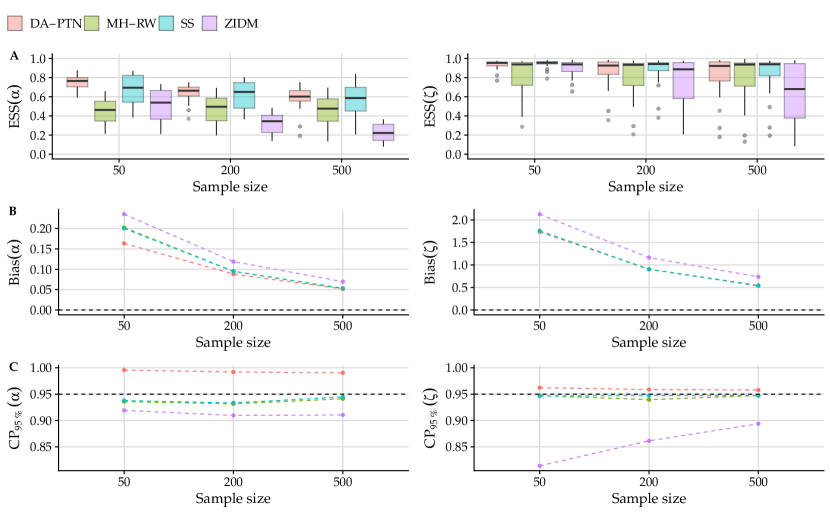
Figure 2: Comparison of efficiency and parameter recovery of the $\bm{\alpha}$ (left) and $\bm{\zeta}$ (right) parameters for different ZANIDM inference schemes. All metrics are averaged over the $d=20$ categories and $R=50$ replicates simulated from ZANIDM with $N=200$ trials and varying sample size $\{50,200,500\}$. A: effective sample size ratio; B: overall relative bias based on the posterior mean; C: overall coverage probability of the $95\%$ credible interval.

The results with lower ($N=50$) and higher ($N=500$) numbers of trials are omitted for brevity. The conclusions about the performance of each inference scheme across all three metics are broadly in line with those drawn from Figure 2. As $N$ varies, only the magnitude of the bias changes; the other metrics are stable and the relative rankings of each approach are unchanged.

5.2 Simulated data analysis examples

This simulation exercise shows the utility of both distributions for addressing zero-inflation in count-compositional data. We simulate two data sets, each containing $500$ observations. The data-generating processes (DGPs) are based on the ZANIM and ZANIDM models, following their respective stochastic representations given in Proposition 2.3 and Definition 2.4. As the parameter values used here match those in Figure 1, Table 1, and Table 2, they are particularly challenging. Specifically, we have $\bm{\theta}=(0.05,0.70,0.25)$ under ZANIM and $\bm{\alpha}=(2.0,28.0,10.0)$ under ZANIDM, with $\bm{\zeta}=(0.05,0.15,0.10)$ and $N=30$ trials in each case.

When fitting ZANIM, we run our MCMC scheme for $11{,}000$ iterations, with the first $1{,}000$ discarded as burn-in and a thinning interval of $10$ applied, and specify the following priors: $\lambda_{j}\sim\operatorname{Gamma}[0.1,0.1]$ and $\zeta_{j}\sim\operatorname{Beta}[1,1]$. For ZANIDM, we run our MCMC scheme for $110{,}000$ iterations, with the first $10{,}000$ discarded as burn-in and a thinning interval of $100$ applied. This setup helps to ensure reliable posterior inference and reduce autocorrelation in the $\bm{\alpha}$ chains, in particular. The prior for $\zeta_{j}$ is set as per the ZANIM model and we use the DA-PTN approach to infer $\alpha_{j}$, with its $\operatorname{Gamma}[c_{j},d_{j}]$ prior elicited as per Section 5.1. Table 3 presents the posterior summaries for the model parameters.

Table 3: Posterior summaries of ZANIM and ZANIDM under both data-generating processes.

DGP	Model	Parameter	Mean	$95\%$ LCI	$95\%$ UCI	ESS ratio
ZANIM: $\bm{\theta}=(0.05,0.70,0.25),$ $\bm{\zeta}=(0.05,0.15,0.10)$, and $N=30$ trials.	ZANIM	$\theta_{1}$	0.047	0.044	0.051	0.808
		$\theta_{2}$	0.706	0.698	0.714	1.037
		$\theta_{3}$	0.246	0.239	0.253	1.039
		$\zeta_{1}$	0.025	0.001	0.070	0.489
		$\zeta_{2}$	0.140	0.111	0.172	0.930
		$\zeta_{3}$	0.122	0.096	0.151	0.833
2-8	ZANIDM	$\alpha_{1}$	3.859	1.456	13.026	0.054
		$\alpha_{2}$	56.607	18.809	219.522	0.055
		$\alpha_{3}$	19.734	6.735	72.113	0.054
		$\zeta_{1}$	0.011	0.000	0.050	0.581
		$\zeta_{2}$	0.140	0.112	0.171	0.933
		$\zeta_{3}$	0.120	0.094	0.151	0.865
ZANIDM: $\bm{\alpha}=(2.0,28.0,10.0),$ $\bm{\zeta}=(0.05,0.15,0.10)$, and $N=30$ trials.	ZANIM	$\theta_{1}$	0.053	0.049	0.058	0.989
		$\theta_{2}$	0.693	0.684	0.702	1.140
		$\theta_{3}$	0.254	0.247	0.262	1.064
		$\zeta_{1}$	0.205	0.148	0.258	0.915
		$\zeta_{2}$	0.127	0.100	0.156	0.812
		$\zeta_{3}$	0.096	0.073	0.122	1.032
2-8	ZANIDM	$\alpha_{1}$	1.241	0.787	2.301	0.148
		$\alpha_{2}$	18.822	11.284	35.420	0.145
		$\alpha_{3}$	6.829	4.130	12.985	0.133
		$\zeta_{1}$	0.025	0.001	0.095	0.476
		$\zeta_{2}$	0.129	0.101	0.160	0.902
		$\zeta_{3}$	0.093	0.068	0.120	0.827

Notably, both models closely recover the true values of the zero-inflation parameters $\bm{\zeta}$ when the data are generated from ZANIM. However, while the inference for $\bm{\theta}$ under ZANIM is satisfactory, the inference for $\bm{\alpha}$ under ZANIDM is poor, as indicated by wide credible intervals and low ESS ratios. Conversely, when the data are generated from ZANIDM, inference for $\bm{\zeta}$ under the ZANIM model is poor, with $\zeta_{1}$ being notably overestimated. This can be attributed to the overdispersion produced by ZANIDM. Inference for $\bm{\alpha}$ under the ZANIDM model is improved in this case, with the true values falling within the 95% credible intervals and larger ESS ratios for $\bm{\alpha}$ compared to the case with ZANIM as the DGP. We note that similar results for the ZANIDM model were obtained using the alternative MH-RW and slice sampling approaches, though ZIDM differs more substantially. For brevity, we defer these results, and those for additional simulations with balanced parameter settings, to the Supplementary Material.

To further compare the models, we compute the expected log-predictive density/mass (ELPD) to evaluate the log-probability mass functions of ZANIM and ZANIDM derived in Section 2. We stress that such likelihood-based model-selection criteria would not be feasible without first deriving these finite mixture PMFs. We use the Pareto smoothed importance sampling (PSIS) introduced by Vehtari et al. [17] and available via the R package loo. Given the posterior draws of the model parameters, denoted by $\{\bm{\vartheta}^{(m)}\}_{m=1}^{M}$, where $m=1,\ldots,M$ indexes the number of valid posterior samples, the estimate of ELPD based on PSIS is defined by

$$\widehat{\operatorname{elpd}}=\sum_{i=1}^{n}\log\left(\dfrac{\sum_{m=1}^{M}w_{i}^{(m)}p(y_{i}\mid\bm{\vartheta}^{(m)})}{\sum_{m=1}^{M}w_{i}^{(m)}}\right),$$

where $w_{i}^{(m)}$ are the PSIS weights and $p(y_{i}\mid\bm{\vartheta}^{(m)})$ is the model likelihood evaluated at the observation $y_{i}$. The higher the ELPD, the better the model.

Table 4 gives the ELPD results for different models and both DGPs. We also include the multinomial and DM distributions for comparison purposes, for which we use Stan via the R package cmdstanr [18] in each case. As expected, the ELPD favours the model used to generate the data, although ZANIDM obtains a similar ELPD to ZANIM when the data are generated from ZANIM. Interestingly, when the data are generated from ZANIDM, we observe that ZANIM outperforms the DM model, suggesting that accounting for zero-inflation improves the fit more than the overdispersion which distinguishes the DM and multinomial distributions. However, we note that the $\mathrm{DI}[Y_{j}]$ indices are similar for both DGPs (see Table 1).

Table 4: Expected log-predictive density/mass $(\widehat{\operatorname{elpd}})$ and its standard error ($\operatorname{se}(\widehat{\operatorname{elpd}})$) for different models with data simulated under different data-generating processes.

DGP	Model	$\widehat{\operatorname{elpd}}$	$\operatorname{se}(\widehat{\operatorname{elpd}})$
ZANIM	ZANIM	$-2051.199$	20.499
	ZANIDM	$-2085.094$	14.126
	DM	$-2749.009$	25.796
	Multinomial	$-4736.613$	262.969
ZANIDM	ZANIDM	$-2201.241$	19.684
	ZANIM	$-2298.938$	34.754
	DM	$-2656.433$	27.609
	Multinomial	$-4749.662$	264.850

For both ZANIM and ZANIDM, each panel in Figure 3 illustrates the mean and the $95\%$ CI of the posterior predictive distribution (represented by red and blue error bars) compared with the empirical distribution of the observed count $Y_{j}$ (depicted by grey bars) for each category $j=1,2,3$. To enhance the visualisation, we report the relative frequency and compare empirical and posterior estimates thereof. In Panel A, the data are generated from ZANIM and, as expected, the fitted ZANIM model closely aligns with the observed data. In contrast, ZANIDM fails to capture certain patterns, particularly for the component $j=2$. Conversely, when the data-generating process originates from ZANIDM, as shown in Panel B, the ZANIDM model provides a better fit, effectively capturing the behavior of the observed data, while ZANIM markedly deviates from the observed data particularly when $\alpha_{j}$ is large.

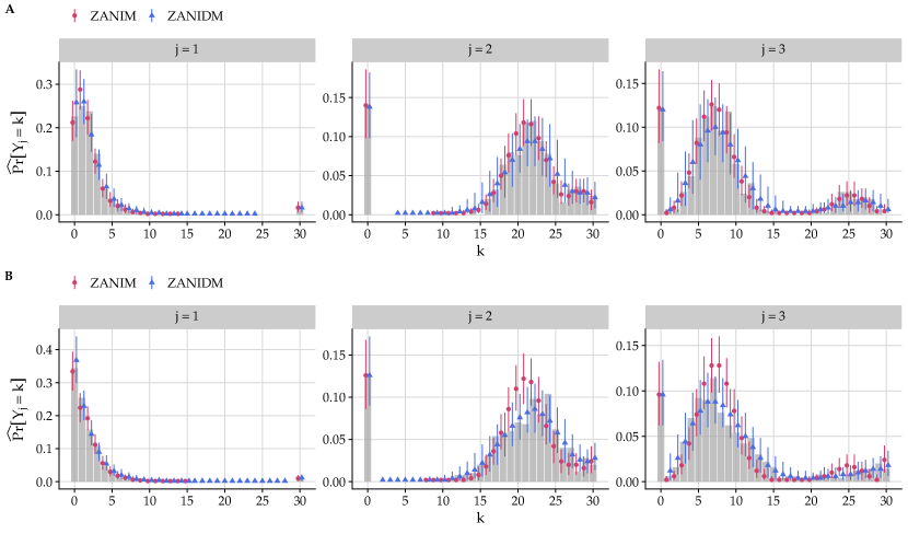
Figure 3: Empirical relative frequency estimates (grey bars) of the observed categories $y_{j}$, with the corresponding model estimates (where available) from the posterior predictive distributions of ZANIM (red circles) and ZANIDM (blue triangles). The points represent the means and the error-bars represent the corresponding $95\%$ prediction intervals. A: DGP from ZANIM. B: DGP from ZANIDM.

6 Discussion

The main contributions of this paper have been the novel probabilistic insights provided for the ZANIM and ZANIDM distributions, which are suitable for addressing zero-inflation in count-compositional data. We provided a probabilistic characterisation of ZANIDM, which was first proposed by Koslovsky [1], and introduced the more parsimonious ZANIM. We demonstrated that both distributions belong to a unifying framework and can be represented as finite mixtures. We derived their key properties, including moments and the corresponding marginal distributions. We showed that the distributions can accommodate overdispersion and positive correlations, which can be attributed to their mixture structure and zero-inflation properties.

We subsequently developed Bayesian inference frameworks for both distributions. Specifically, for ZANIDM, we showed through simulation studies that our collapsed Gibbs sampling approach for updating the latent parameters is more efficient than the algorithm of Koslovsky [1]. Our extensive simulations also showed that both distributions are effective when data exhibit zero-inflation across multiple categories. It is worth noting that if exclusively non-zero counts are observed in one or more categories, or if contextual information gives sufficient reason to believe that the observed zeros for a given $Y_{j}$ are not structural in nature, we can simplify the distributions by removing the corresponding zero-inflation parameters $\zeta_{j}$ from the model.

Our unifying framework that characterises both distributions as finite mixtures can be extended to incorporate other component distributions suitable for modelling count-compositional data, e.g., the Conway-Maxwell-multinomial distribution [4, 5]. In doing so, novel zero-&-$N$-inflated counterparts for such distributions could be developed, though inference would remain a challenge. Compositional distributions that handle proportions, such as the Dirichlet distribution, could also be extended in a similar fashion.

Another interesting avenue for future research would be to explore non-parametric regression approaches for incorporating covariates into the category-specific parameters of both distributions. For ZANIM, this would extend the approach of Zeng et al. [10], who allow only the success probabilities, and not the zero-inflation parameters, to depend on covariates. For ZANIDM, this would provide additional flexibility over the log-linear and logistic regressions employed by Koslovsky [1] for the $\alpha_{j}$ and $\zeta_{j}$ parameters, respectively. We also stress that, even in regression settings, our Gibbs updates of $\lambda_{ij}$ and $z_{ij}$ under ZANIDM would still be advantageous.

Overall, we envisage that the novel theoretical insights we provide for ZANIM and ZANIDM will be of interest to researchers and applied practitioners working with either distribution or with zero-inflated multivariate data more broadly.

Appendices

Appendix A Derivation of the ZANIM PMF

Proof of Proposition 2.1.

The goal is to marginalise out the latent variable $\phi$ from Equation (6) and ensure that the function $\int\Pr[\mathbf{Y}=\mathbf{y},\phi;\bm{\lambda},\bm{\zeta}]\mathop{}\!\mathrm{d}\phi$ will be a proper PMF. We shall denote $\Pr[\mathbf{Y}=\mathbf{y},\phi;\bm{\lambda},\bm{\zeta}]=p(\mathbf{y},\phi)$, for brevity. We begin with

$$p(\mathbf{y},\phi)=\dfrac{N!\,\phi^{N-1}}{\Gamma(N)}\,\prod_{j=1}^{d}\left[\zeta_{j}\,\mathds{1}_{0}(y_{j})+(1-\zeta_{j})\,\dfrac{\lambda_{j}^{y_{j}}\,e^{-\lambda_{j}\,\phi}}{y_{j}!}\right],$$

and note that the product will have $2^{d}$ terms, as a consequence of the binomial theorem. However, due to the indicator function $\mathds{1}_{0}(y_{j})$, we can simplify some terms. We shall consider four different groups of terms, corresponding to the four types of mixture component in ZANIM.

$\bullet$ Standard multinomial$\colon$

$$\int p(\mathbf{y},\phi)\mathop{}\!\mathrm{d}\phi =\int\dfrac{N!\,\phi^{N-1}}{\Gamma(N)}\,\prod_{j=1}^{d}\left[(1-\zeta_{j})\,\dfrac{\lambda_{j}^{y_{j}}\,e^{-\lambda_{j}\,\phi}}{y_{j}!}\right]\mathop{}\!\mathrm{d}\phi$$

$$=\displaystyle\binom{N}{y_{1}\dots y_{d}}\left[\prod_{j=1}^{d}\,(1-\zeta_{j})\,\lambda_{j}^{y_{j}}\right]\int\dfrac{1}{\Gamma(N)}\,\phi^{N-1}\,e^{-\phi\,\sum_{j=1}^{d}\,\lambda_{j}}\mathop{}\!\mathrm{d}\phi$$

$$=\displaystyle\binom{N}{y_{1}\dots y_{d}}\,\prod_{j=1}^{d}\,(1-\zeta_{j})\,\left(\dfrac{\lambda_{j}}{\sum_{k=1}^{d}\lambda_{k}}\right)^{y_{j}}=\displaystyle\binom{N}{y_{1}\dots y_{d}}\,\prod_{j=1}^{d}\,(1-\zeta_{j})\,\theta_{j}^{y_{j}}.$$

$\bullet$ $\delta_{\mathbf{0}_{d}}$ component$\colon$

$$\int p(\mathbf{y},\phi)\mathop{}\!\mathrm{d}\phi =\left[\prod_{j=1}^{d}\,\zeta_{j}\,\mathds{1}_{0}(y_{j})\right]\,N!\,\int\dfrac{1}{\Gamma(N)}\,\phi^{N-1}\,\mathop{}\!\mathrm{d}\phi$$

$$=\left[\prod_{j=1}^{d}\,\zeta_{j}\,\mathds{1}_{0}(y_{j})\right]\,N!\,\int\dfrac{1}{\Gamma(N)}\,\phi_{i}^{N-1}\,e^{-0\,\phi}\,0^{N-N}\mathop{}\!\mathrm{d}\phi$$

$$=\left[\prod_{j=1}^{d}\,\zeta_{j}\,\mathds{1}_{0}(y_{j})\right]\,0!\,0^{0}\int\dfrac{1}{\Gamma(N)}\,\phi^{N-1}\,e^{-0\,\phi}\,0^{N}\mathop{}\!\mathrm{d}\phi,$$

since $N=0$ when $y_{j}=0\>\forall\>j$, such that $N!=0!=1$, and $0^{0}=1$, by convention. The integral above is an abstract representation of a $\operatorname{Gamma}[0,0]$ distribution, which in practice is not well-defined. Here, we shall adopt the convention that $\operatorname{Gamma}[0,0]\overset{d}{=}\delta_{0}(\cdot)$. Under this convention, the distribution is a point-mass at $0$ with probability $1$, whose integral evaluates to $1$. Thus, $\int p(\mathbf{y},\phi)\mathop{}\!\mathrm{d}\phi=\prod_{j=1}^{d}\,\zeta_{j}\,\mathds{1}_{0}(y_{j}).$

$\bullet$ $\mathbf{E}_{d}^{(j)}$ components$\colon$ We have $d$ terms with this constraint, which can be written as follows:

$$\int p(\mathbf{y},\phi)\mathop{}\!\mathrm{d}\phi =\sum_{j=1}^{d}\left\{\mathds{1}_{0}\left(\sum_{k\colon k\neq j}y_{k}\right)(1-\zeta_{j})\prod_{k\colon k\neq j}\zeta_{k}\int\dfrac{N!\,\phi^{N-1}}{\Gamma(N)}\dfrac{\lambda_{j}^{y_{j}}\,e^{-\lambda_{j}\phi}}{y_{j}!}\mathop{}\!\mathrm{d}\phi\right\}$$

$$=\sum_{j=1}^{d}\left\{\mathds{1}_{0}\left(\sum_{k\colon k\neq j}y_{k}\right)(1-\zeta_{j})\prod_{k\colon k\neq j}\zeta_{k}\,\dfrac{\lambda_{j}^{y_{j}}\,N!}{y_{j}!}\int\dfrac{e^{-\lambda_{j}\phi}\phi^{N-1}}{\Gamma(N)}\mathop{}\!\mathrm{d}\phi\right\}$$

$$=\sum_{j=1}^{d}\left\{\mathds{1}_{0}\left(\sum_{k\colon k\neq j}y_{k}\right)(1-\zeta_{j})\prod_{k\colon k\neq j}\zeta_{k}\right\},$$

where the simplification comes from the fact that $N=y_{j}$ when $y_{j}>0$ and $y_{k}=0$ $\forall\>k\neq j$.

$\bullet$ Reduced multinomials$\colon$ The remaining terms represent cases where at most $d-2$ categories exhibit zero-inflation. To write the $2^{d}-d-2$ such terms compactly, we define the corresponding set $\mathfrak{K}$ as follows. Let $\mathfrak{K}=\{\mathcal{K}\subseteq\{1,\ldots,d\};1\leq\lvert\mathcal{K}\rvert\leq d-2\}$. Then, $\mathfrak{K}$ consists of mutually exclusive sets $\mathcal{K}$, where $\mathcal{K}\subseteq\{1,\ldots,d\}$, with $1\leq\lvert\mathcal{K}\rvert\leq d-2$, i.e., all subsets $\mathcal{K}$ of the category indices $\{1,\ldots,d\}$ with cardinality between $1$ and $d-2$ inclusive. Using this, we can write

$$p(\mathbf{y},\phi)=\dfrac{N!\,\phi^{N-1}}{\Gamma(N)}\sum_{\mathcal{K}\in\mathfrak{K}}\left\{\mathds{1}_{0}\left(\sum_{k\in\mathcal{K}}y_{k}\right)\prod_{k\in\mathcal{K}}\zeta_{k}\prod_{j\notin\mathcal{K}}\left[(1-\zeta_{j})\dfrac{\lambda_{j}^{y_{j}}\,e^{-\lambda_{j}\phi}}{y_{j}!}\right]\right\}.$$

Then, for a generic set $\mathcal{K}$, we have

$$\int p(\mathbf{y},\phi)\mathop{}\!\mathrm{d}\phi =\mathds{1}_{0}\left(\sum_{k\in\mathcal{K}}y_{k}\right)\prod_{k\in\mathcal{K}}\zeta_{k}\prod_{j\notin\mathcal{K}}\left[(1-\zeta_{j})\dfrac{\lambda_{j}^{y_{j}}}{y_{j}!}\right]N!\,\int\dfrac{e^{-\phi\sum_{j\notin\mathcal{K}}\lambda_{j}}\phi^{N-1}}{\Gamma(N)}\mathop{}\!\mathrm{d}\phi$$

$$=\mathds{1}_{0}\left(\sum_{k\in\mathcal{K}}y_{k}\right)\prod_{k\in\mathcal{K}}\zeta_{k}\prod_{j\notin\mathcal{K}}\left[(1-\zeta_{j})\dfrac{\lambda_{j}^{y_{j}}}{y_{j}!}\right]N!\left(\sum_{j\notin\mathcal{K}}\lambda_{j}\right)^{-N}$$

$$=\mathds{1}_{0}\left(\sum_{k\in\mathcal{K}}y_{k}\right)\prod_{k\in\mathcal{K}}\zeta_{k}\prod_{j\notin\mathcal{K}}\left[(1-\zeta_{j})\right]\binom{N}{\{y_{j}\}_{j\notin\mathcal{K}}}\prod_{j\notin\mathcal{K}}\left[\left(\theta_{j}^{\mathcal{K}}\right)^{y_{j}}\right],$$

where $\theta_{j}^{\mathcal{K}}=\lambda_{j}/\sum_{k\notin\mathcal{K}}\lambda_{k}=\theta_{j}/(1-\sum_{k\in\mathcal{K}}\theta_{k})$. The simplification arises from the fact that we have $y_{k}=0$ for the indices $k\in\mathcal{K}$, such that $N=\sum_{j=1}^{d}\,y_{j}=\sum_{j\notin\mathcal{K}}y_{j}$.

Collecting the terms and using Definition 2.2 leads to Proposition 2.1. ∎

Appendix B Derivation of the ZANIDM PMF

Proof of Proposition 2.4.

From the stochastic representation in Definition 2.4, we highlight a key fact that will be used extensively below, which is that $\lambda_{j}=0$ (i.e., $z_{j}=0$) implies $y_{j}=0$. Next, we note that we can marginalise out $z_{j}$ in the distribution of the latent $\lambda_{j}\in\{0,\mathbb{R}^{+}\}$ via

$$p(\lambda_{j}\mid\alpha_{j},\zeta_{j})=\sum_{k=0}^{1}p(\lambda_{j}\mid z_{j}=k,\alpha_{j})\,p(z_{j}=k\mid\zeta_{j})=\zeta_{j}\,\delta_{0}(\lambda_{j})+(1-\zeta_{j})\dfrac{\lambda_{j}^{\alpha_{j}-1}e^{-\lambda_{j}}}{\Gamma(\alpha_{j})}.$$

Consequently, we note that $(\lambda_{j}\mid\alpha_{j},\zeta_{j})\sim\operatorname{ZAG}[1-\zeta_{j},\alpha_{j},1]$, i.e., unconditional on $z_{j}$, the latent variable $\lambda_{j}$ follows a zero-augmented gamma distribution with shape $\alpha_{j}$, rate $1$, and $\zeta_{j}$ being the probability that $\lambda_{j}=0$. Thus, the probability density function of $(\lambda_{j}\mid\alpha_{j},\zeta_{j})$ is given by:

$$p(\lambda_{j}\mid\zeta_{j},\alpha_{j})=\zeta_{j}^{\mathds{1}_{0}(\lambda_{j})}\,(1-\zeta_{j})^{1-\mathds{1}_{0}(\lambda_{j})}\,\left(\dfrac{\lambda_{j}^{\alpha_{j}-1}\,e^{-\lambda_{j}}}{\Gamma(\alpha_{j})}\right)^{1-\mathds{1}_{0}(\lambda_{j})},\quad\lambda_{j}\in\{0,\mathbb{R}^{+}\}.$$

Note that the augmented likelihood for the ZANIDM distribution can be written as

$$\mathcal{L}(\mathbf{y},\bm{\lambda};\bm{\alpha},\bm{\zeta}) =\binom{N}{y_{1},\ldots,y_{d}}\,\prod_{j=1}^{d}\left(\frac{\lambda_{j}}{\sum_{k=1}^{d}\,\lambda_{k}}\right)^{y_{j}}\left[\zeta_{j}^{\mathds{1}_{0}(\lambda_{j})}\,(1-\zeta_{j})^{1-\mathds{1}_{0}(\lambda_{j})}\left(\frac{\lambda_{j}^{\alpha_{j}-1}e^{-\lambda_{j}}}{\Gamma(\alpha_{j})}\right)^{1-\mathds{1}_{0}(\lambda_{j})}\right]$$

$$=c\prod_{j=1}^{d}\left[\zeta_{j}^{\mathds{1}_{0}(\lambda_{j})}\,(1-\zeta_{j})^{1-\mathds{1}_{0}(\lambda_{j})}\,\right]\prod_{j=1}^{d}\left[\left(\frac{\lambda_{j}}{\sum_{k=1}^{d}\,\lambda_{k}}\right)^{y_{j}}\left(\frac{\lambda_{j}^{\alpha_{j}-1}e^{-\lambda_{j}}}{\Gamma(\alpha_{j})}\right)^{1-\mathds{1}_{0}(\lambda_{j})}\right]$$

$$=c\prod_{j=1}^{d}\left[\zeta_{j}^{\mathds{1}_{0}(\lambda_{j})}\,(1-\zeta_{j})^{1-\mathds{1}_{0}(\lambda_{j})}\,\right]\prod_{j=1}^{d}\left[\left(\frac{1}{\sum_{k=1}^{d}\,\lambda_{k}}\right)^{y_{j}}\left(\frac{\lambda_{j}^{y_{j}+\alpha_{j}-1}e^{-\lambda_{j}}}{\Gamma(\alpha_{j})}\right)\right]^{1-\mathds{1}_{0}(\lambda_{j})},$$

where we denote the constant $c=\binom{N}{y_{1},\ldots,y_{d}}=\Gamma(N+1)/\prod_{j=1}^{d}\Gamma(y_{j}+1)$, for simplicity, and the simplification in the last expression relies on $\theta_{j}^{y_{j}}$ being non-zero when $\lambda_{j}>0$. In light of this, the marginal PMF of $\mathbf{Y}$ is obtained by integrating out the latent variables $\lambda_{j}$:

$$p(\mathbf{y}\mid\bm{\alpha},\bm{\zeta})=\int\ldots\int\mathcal{L}(\mathbf{y},\bm{\lambda};\bm{\alpha},\bm{\zeta})\mathop{}\!\mathrm{d}\lambda_{1}\ldots\mathop{}\!\mathrm{d}\lambda_{d}.$$

Before we proceed with the integration, we state the integral result; consider the change of variables $s=\sum_{j=1}^{d}\,\lambda_{j}$ and $\lambda_{j}=\theta_{j}\,s$, which leads to $\mathop{}\!\mathrm{d}\lambda_{1}\ldots\mathop{}\!\mathrm{d}\lambda_{d}=s^{d-1}\,\mathop{}\!\mathrm{d}s\,\prod_{j=1}^{d-1}\,\mathop{}\!\mathrm{d}\theta_{j}$. Note that the vector $\bm{\theta}=(\theta_{1},\ldots\theta_{d})$ belongs to the simplex $\mathcal{S}^{d}=\{\bm{\theta}:\theta_{j}>0,j=1,\ldots,d,\sum_{j=1}^{d}\theta_{j}=1\}$, which leads to the following multivariate beta integral result:

$$\int_{\mathcal{S}^{d}}\prod_{j=1}^{d}\theta_{j}^{k_{j}-1}\mathop{}\!\mathrm{d}\bm{\theta}=\int_{0}^{1}\,\int_{0}^{1-\theta_{1}}\ldots\int_{0}^{1-\theta_{1}-\ldots-\theta_{d-2}}\theta_{1}^{k_{1}-1}\ldots\theta_{d}^{k_{d}-1}\mathop{}\!\mathrm{d}\theta_{1}\,\ldots\mathop{}\!\mathrm{d}\theta_{d-1}=\dfrac{\prod_{j=1}^{d}\,\Gamma(k_{j})}{\Gamma(\sum_{j=1}^{d}\,k_{j})},$$

where we do not need to integrate with respect to $\theta_{d}$ explicitly, since $\theta_{d}$ is fully determined by the simplex constraint $\sum_{j=1}^{d}\theta_{j}=1$. Since $\lambda_{j}\in\{0,\mathbb{R}^{+}\}\>\forall\>j=1,\ldots,d$, the integration should be performed considering all $2^{d}$ combinations of $\lambda_{j}$ being $0$ or non-zero. We consider four different groups of terms, as per A, and denote $\alpha_{s}=\sum_{j=1}^{d}\,\alpha_{j}$, $\alpha^{\mathcal{K}}_{s}=\sum_{j\notin\mathcal{K}}\alpha_{j}$.

$\bullet$ No inflation$\colon$ When $\lambda_{j}>0\>\forall\>j$, then the integral becomes

$$\int\ldots\int c\prod_{j=1}^{d}\left[\zeta_{j}^{\mathds{1}_{0}(\lambda_{j})}\,(1-\zeta_{j})^{1-\mathds{1}_{0}(\lambda_{j})}\,\right]\prod_{j=1}^{d}\left[\left(\frac{1}{\sum_{k=1}^{d}\,\lambda_{k}}\right)^{y_{j}}\left(\frac{\lambda_{j}^{y_{j}+\alpha_{j}-1}e^{-\lambda_{j}}}{\Gamma(\alpha_{j})}\right)\right]^{1-\mathds{1}_{0}(\lambda_{j})}\mathop{}\!\mathrm{d}\lambda_{1}\ldots\mathop{}\!\mathrm{d}\lambda_{d}$$

$$=c\prod_{j=1}^{d}\,(1-\zeta_{j})\times\int\ldots\int\prod_{j=1}^{d}\left[\left(\frac{1}{\sum_{k=1}^{d}\,\lambda_{k}}\right)^{y_{j}}\left(\frac{\lambda_{j}^{y_{j}+\alpha_{j}-1}e^{-\lambda_{j}}}{\Gamma(\alpha_{j})}\right)\right]\mathop{}\!\mathrm{d}\lambda_{1}\ldots\mathop{}\!\mathrm{d}\lambda_{d}$$

$$=c\prod_{j=1}^{d}\,(1-\zeta_{j})\,\dfrac{\Gamma(\alpha_{s})}{\Gamma(N+\alpha_{s})}\,\prod_{j=1}^{d}\,\dfrac{\Gamma(y_{j}+\alpha_{j})}{\Gamma(\alpha_{j})}=\dfrac{\Gamma(N+1)\Gamma(\alpha_{s})}{\Gamma(N+\alpha_{s})}\,\prod_{j=1}^{d}\,(1-\zeta_{j})\dfrac{\Gamma(y_{j}+\alpha_{j})}{\Gamma(\alpha_{j})\Gamma(y_{j}+1)}.$$

$\bullet$ ‘All’-inflation$\colon$ When $\lambda_{j}=0\>\forall\>j$, then $y_{j}=0\>\forall\>j$ and $c=1$, such that the integral becomes

$$\int\ldots\int c\prod_{j=1}^{d}\left[\zeta_{j}^{\mathds{1}_{0}(\lambda_{j}+{y_{j}})}\,(1-\zeta_{j})^{1-\mathds{1}_{0}(\lambda_{j})}\,\right]\prod_{j=1}^{d}\left[\left(\frac{1}{\sum_{k=1}^{d}\,\lambda_{k}}\right)^{y_{j}}\left(\frac{\lambda_{j}^{y_{j}+\alpha_{j}-1}e^{-\lambda_{j}}}{\Gamma(\alpha_{j})}\right)\right]^{1-\mathds{1}_{0}(\lambda_{j})}\mathop{}\!\mathrm{d}\lambda_{1}\ldots\mathop{}\!\mathrm{d}\lambda_{d}$$

$$=\prod_{j=1}^{d}\zeta_{j}.$$

$\bullet$ $N$-inflation$\colon$ When $\lambda_{k}=0\>\forall\>k\neq j$, we know that $y_{k}=0\>\forall\>k\neq j$, such that $c=1$, since $N=y_{j}$. Note that we have $d$ terms with this constraint. We can write these terms as follows

$$\int\ldots\int c\prod_{j=1}^{d}\left[\zeta_{j}^{\mathds{1}_{0}(\lambda_{j})}\,(1-\zeta_{j})^{1-\mathds{1}_{0}(\lambda_{j})}\,\right]\prod_{j=1}^{d}\left[\left(\frac{1}{\sum_{k=1}^{d}\,\lambda_{k}}\right)^{y_{j}}\left(\frac{\lambda_{j}^{y_{j}+\alpha_{j}-1}e^{-\lambda_{j}}}{\Gamma(\alpha_{j})}\right)\right]^{1-\mathds{1}_{0}(\lambda_{j})}\mathop{}\!\mathrm{d}\lambda_{1}\ldots\mathop{}\!\mathrm{d}\lambda_{d}$$

$$=c\prod_{k\neq j}\zeta_{k}\,(1-\zeta_{j})\int\left(\frac{1}{\lambda_{j}}\right)^{y_{j}}\left(\frac{\lambda_{j}^{y_{j}+\alpha_{j}-1}e^{-\lambda_{j}}}{\Gamma(\alpha_{j})}\right)\mathop{}\!\mathrm{d}\lambda_{j}$$

$$=c\prod_{k\neq j}\,\zeta_{k}\,(1-\zeta_{j})\int\frac{\lambda_{j}^{\alpha_{j}-1}e^{-\lambda_{j}}}{\Gamma(\alpha_{j})}\mathop{}\!\mathrm{d}\lambda_{j}=(1-\zeta_{j})\,\prod_{k\neq j}\,\zeta_{k}.$$

$\bullet$ Sets of inflation$\colon$ Similar to the derivation of the ZANIM PMF in A, the remaining terms represent cases where at most $d-2$ categories from $\{1,\ldots,d\}$ exhibit zero-inflation. Note that there are $2^{d}-d-2$ such terms. To write them compactly, we recall the definition $\mathfrak{K}=\{\mathcal{K}\subseteq\{1,\ldots,d\};1\leq\lvert\mathcal{K}\rvert\leq d-2\}$. For a given $\mathcal{K}\in\mathfrak{K}$, we know when $\lambda_{k}=0$ for all $k\in\mathcal{K}$ that $y_{k}=0\>\forall\>k\in\mathcal{K}$ and that $\lambda_{j}=0$ for all $j\notin\mathcal{K}$. Hence, we have

$$\int\ldots\int c\prod_{j=1}^{d}\left[\zeta_{j}^{\mathds{1}_{0}(\lambda_{j}+{y_{j}})}\,(1-\zeta_{j})^{1-\mathds{1}_{0}(\lambda_{j})}\,\right]\prod_{j=1}^{d}\left[\left(\frac{1}{\sum_{k=1}^{d}\,\lambda_{k}}\right)^{y_{j}}\left(\frac{\lambda_{j}^{y_{j}+\alpha_{j}-1}e^{-\lambda_{j}}}{\Gamma(\alpha_{j})}\right)\right]^{1-\mathds{1}_{0}(\lambda_{j})}\mathop{}\!\mathrm{d}\lambda_{1}\ldots\mathop{}\!\mathrm{d}\lambda_{d}$$

$$=c\prod_{k\in\mathcal{K}}\,\zeta_{k}\,\prod_{j\notin\mathcal{K}}\,(1-\zeta_{j})\,\int\prod_{j\notin\mathcal{K}}\left[\left(\frac{1}{\sum_{\ell\notin\mathcal{K}}\,\lambda_{\ell}}\right)^{y_{j}}\frac{\lambda_{j}^{y_{j}+\alpha_{j}-1}e^{-\lambda_{j}}}{\Gamma(\alpha_{j})}\right]\bm{\mathop{}\!\mathrm{d}}\bm{\lambda}^{(\mathcal{K})}$$

$$=\dfrac{\Gamma(\alpha^{\mathcal{K}}_{s})\Gamma(N+1)}{\Gamma(N+\alpha^{\mathcal{K}}_{s})}\,\prod_{k\in\mathcal{K}}\zeta_{h}\,\prod_{j\notin\mathcal{K}}\,(1-\zeta_{j})\,\dfrac{\Gamma(y_{j}+\alpha_{j})}{\Gamma(\alpha_{j})\Gamma(y_{j}+1)},$$

where the multivariate integral is over the set $\bm{\lambda}^{(\mathcal{K})}=\{\lambda_{j}\colon\lambda_{j}\notin\mathcal{K}\}$.

Collecting the terms while accounting for the restriction that $y_{j}=0$ when $\lambda_{j}=0$ and using Definition 2.2 leads to Proposition 2.4. ∎

Supplementary Material

Supp. Mat. A ZANIM inference via data augmentation

Inference for ZANIM is based on the augmented likelihood $p(\mathbf{y},\phi,\bm{z)}=p(\phi\mid\mathbf{y},\mathbf{z})\,p(\mathbf{y}\mid\mathbf{z})\,p(\mathbf{z})$. We establish the validity of this approach by showing how the augmented likelihood in Equation (6), from which ZANIM was derived, can be recovered from this expression. For this derivation, we adopt the notation $c=\binom{N}{y_{1}\cdots y_{d}}$ and drop the subscript $i$, for simplicity.

Let $\mathbf{z}=(z_{1},\ldots,z_{d})$, where $z_{j}=0$ corresponds to a structural zero count and $z_{j}=1$ represents a count obtained from a sampling distribution (which may also be zero). Assuming $z_{j}\sim\operatorname{Bernoulli}\left[1-\zeta_{j}\right]$ and independence over $j=1,\ldots,d$, we have $p(\mathbf{z})=\prod_{j=1}^{d}(1-\zeta_{j})^{z_{j}}\,\zeta_{j}^{1-z_{j}}$. Conditional on $\mathbf{z}$, we can fully determine which one of the $2^{d}$ mixture components from ZANIM that $\mathbf{y}$ belongs to. This is important because we do not need to use the common mixture model data augmentation which requires $K=2^{d}$ latent variables. Thus, we introduce a latent variable, conditional on $\mathbf{z}$, given by $(\phi\mid\mathbf{y},\mathbf{z})\sim\operatorname{Gamma}[N,\sum_{j=1}^{d}\lambda_{j}\,z_{j}]$. This is similar to the data augmentation given in Equation (2), though here the contributions of structural zeros are removed from the calculation of the rate parameter. As per A, we consider four groups of terms, corresponding to the four types of mixture component in ZANIM.

$\bullet$ Standard multinomial component$\colon$ For this component, we have that $\mathbf{z}=\mathbf{1}_{d}$ and

$$c\prod_{j=1}^{d}\left\{\left(\dfrac{\lambda_{j}}{\sum_{k=1}^{d}\lambda_{k}}\right)^{y_{j}}\right\}\dfrac{\phi^{N-1}}{\Gamma(N)}\exp\left[-\phi\sum_{j=1}^{d}\lambda_{j}\,z_{j}\right]\left(\sum_{j=1}^{d}\lambda_{j}\,z_{j}\right)^{N}\prod_{j=1}^{d}\Pr[z_{j}=1]\mathds{1}(z_{j}=1)$$

$$=c\dfrac{\phi^{N-1}}{\Gamma(N)}\prod_{j=1}^{d}\left\{(1-\zeta_{j})\lambda_{j}^{y_{j}}e^{-\phi\lambda_{j}}\mathds{1}(z_{j}=1)\right\},\vskip-3.0pt plus -1.0pt minus -1.0pt$$

where some simplification arises from the fact that $N=\sum_{j=1}^{d}y_{j}$.

$\bullet$ $\delta_{\mathbf{0}_{d}}$ component$\colon$ For this component, we have $\mathbf{z}=\mathbf{0}_{d}$ and, subject to some simplifications,

$$c\prod_{j=1}^{d}\mathds{1}_{0}(y_{j})\times\dfrac{\phi^{N-1}}{\Gamma(N)}\,e^{-0\,\phi}\,0^{0}\times\Pr[z_{j}=0]\mathds{1}_{0}(z_{j})=c\dfrac{\phi^{N-1}}{\Gamma(N)}\prod_{j=1}^{d}\zeta_{j}\mathds{1}_{0}(y_{j})\mathds{1}_{0}(z_{j}).$$

$\bullet$ $\mathbf{E}_{d}^{(j)}$ components$\colon$ For these components, the vector $\mathbf{z}$ has the value $1$ in one entry only. Suppose the $j$-th entry is $1$, such that $N=y_{j}$ and $y_{k}=0\>\forall\>k\neq j$. We then have

$$c\prod_{k\colon k\neq j}\left\{\mathds{1}_{0}(y_{k})\times\dfrac{\phi^{N-1}}{\Gamma(N)}\exp\left[-\phi\sum_{j=1}^{d}\lambda_{j}z_{j}\right]\left(\sum_{j=1}^{d}\lambda_{j}z_{j}\right)^{N}\times\Pr[z_{k}=0]\mathds{1}_{0}(z_{k})\Pr[z_{j}=1]\mathds{1}(z_{j}=1)\right\}$$

$$=c\dfrac{\phi^{N-1}}{\Gamma(N)}\prod_{k\colon k\neq j}\left\{\zeta_{k}\mathds{1}_{0}(y_{k})\mathds{1}_{0}(z_{k})\right\}\times(1-\zeta_{j})\lambda_{j}^{y_{j}}e^{-\phi\lambda_{j}}\mathds{1}(z_{j}=1).$$

$\bullet$ Reduced multinomial components$\colon$ For these components, the vector $\mathbf{z}$ contains $0$ at the entries $k\in\mathcal{K}$ and $1$ at the entries $j\notin\mathcal{K}$, such that $y_{k}=0\>\forall\>k\in\mathcal{K}$. We then have

$$c\prod_{k\in\mathcal{K}}\mathds{1}_{0}(y_{k})\prod_{j\notin\mathcal{K}}\left[\left(\dfrac{\lambda_{j}}{\sum_{\ell\notin\mathcal{K}}\lambda_{\ell}}\right)^{y_{j}}\right]\times\dfrac{\phi^{N-1}}{\Gamma(N)}\exp\left[-\phi\sum_{j=1}^{d}\lambda_{j}z_{j}\right]\left(\sum_{j=1}^{d}\lambda_{j}z_{j}\right)^{N}$$

$$\phantom{=}~\times\prod_{k\in\mathcal{K}}\Pr[z_{k}=0]\mathds{1}_{0}(z_{k})\prod_{j\notin\mathcal{K}}\Pr[z_{j}=1]\mathds{1}(z_{j}=1)$$

$$=c\prod_{k\in\mathcal{K}}\mathds{1}_{0}(y_{k})\mathds{1}_{0}(z_{k})\zeta_{k}\prod_{j\notin\mathcal{K}}\left[(1-\zeta_{j})\mathds{1}(z_{j}=1)\left(\dfrac{\lambda_{j}}{\sum_{\ell\notin\mathcal{K}}\lambda_{\ell}}\right)^{y_{j}}\right]$$

$$\phantom{=}~\times\dfrac{\phi^{N-1}}{\Gamma(N)}\exp\left[-\phi\sum_{j\notin\mathcal{K}}\lambda_{j}z_{j}\right]\left(\sum_{j\notin\mathcal{K}}\lambda_{j}z_{j}\right)^{N}$$

$$=c\dfrac{\phi^{N-1}}{\Gamma(N)}\prod_{k\in\mathcal{K}}\mathds{1}_{0}(y_{k})\mathds{1}_{0}(z_{k})\zeta_{k}\prod_{j\notin\mathcal{K}}\left[(1-\zeta_{j})\lambda_{j}^{y_{j}}e^{-\phi\lambda_{j}}\mathds{1}(z_{j}=1)\right].$$

By summing over all terms above, where $c^{\prime}=(c\,\phi^{N-1})/\Gamma(N)$ is a common factor, we obtain

$$p(\mathbf{y},\phi,\bm{z)} =c^{\prime}\prod_{j=1}^{d}\left\{(1-\zeta_{j})\lambda_{j}^{y_{j}}e^{-\phi\lambda_{j}}\mathds{1}(z_{j}=1)\right\}+c^{\prime}\prod_{j=1}^{d}\zeta_{j}\mathds{1}_{0}(y_{j})\mathds{1}_{0}(z_{j})$$

$$\phantom{=}~+c^{\prime}\sum_{j=1}^{d}\left[\prod_{k\colon k\neq j}\left\{\zeta_{k}\mathds{1}_{0}(y_{k})\mathds{1}_{0}(z_{k})\right\}\times(1-\zeta_{j})\lambda_{j}^{y_{j}}e^{-\phi\lambda_{j}}\mathds{1}(z_{j}=1)\right]$$

$$\phantom{=}~+c^{\prime}\sum_{\mathcal{K}\in\mathfrak{K}}\left[\prod_{k\in\mathcal{K}}\mathds{1}_{0}(y_{k})\mathds{1}_{0}(z_{k})\zeta_{k}\prod_{j\notin\mathcal{K}}\left[(1-\zeta_{j})\lambda_{j}^{y_{j}}e^{-\phi\lambda_{j}}\mathds{1}(z_{j}=1)\right]\right].$$

We can also factor out the terms $\mathds{1}_{0}(z_{j})\mathds{1}_{0}(y_{j})\zeta_{j}+\mathds{1}(z_{j}=1)(1-\zeta_{j})\lambda_{j}^{y_{j}}\,e^{-\phi_{i}\,\lambda_{j}}$. Then, by noting that $\mathds{1}_{0}(z_{j})=1-z_{j}$ and $\mathds{1}(z_{j}=1)=z_{j}$, we can express the above sum as

$$p(\mathbf{y},\phi,\bm{z)} =c^{\prime}\prod_{j=1}^{d}\left\{\left[(1-z_{j})\zeta_{j}+z_{j}(1-\zeta_{j})e^{-\phi\lambda_{j}}\right]^{\mathds{1}_{0}(y_{j})}\times\left[z_{j}(1-\zeta_{j})\lambda_{j}^{y_{j}}e^{-\phi\lambda_{j}}\right]^{1-\mathds{1}_{0}(y_{j})}\right\}.$$ (S.1)

Importantly, the augmented likelihood factors into separate terms for each category after conditioning on $\mathbf{z}$ and $\phi$. Furthermore, we note that the likelihood contribution within a given category is a product of two terms; one for when $y_{j}=0$ and one for when $y_{j}>0$.

To derive $(\mathbf{z}\mid\mathbf{y},\phi)$, we first note that $p(\mathbf{z}\mid\mathbf{y},\phi)=\prod_{j=1}^{d}p(z_{j}\mid y_{j},\phi)$, since the categories are conditionally independent, as seen by Equation (S.1). For a given category $j$ when $y_{j}>0$, we have that $p(z_{j}\mid y_{j}>0,\phi)\propto z_{j}(1-\zeta_{j})y_{j}^{\lambda_{j}}e^{-\phi\lambda_{j}}$. It is evident that $p(z_{j}=1\mid y_{j}>0,\phi)=1$, hence $(z_{j}\mid y_{j}>0,\phi)$ is a degenerate distribution at $1$ when $y_{j}>0$. On the other hand, when $y_{j}=0$, we have that $p(z_{j}\mid y_{j}=0,\phi)\propto(1-z_{j})\zeta_{j}+z_{j}(1-\zeta_{j})e^{-\phi\lambda_{j}}$. Since $z_{j}\in\{0,1\}$, we obtain

$$p(z_{j}\mid y_{j}=0,\phi)=\dfrac{(1-z_{j})\zeta_{j}+z_{j}(1-\zeta_{j})e^{-\phi\lambda_{j}}}{\zeta_{j}+(1-\zeta_{j})e^{-\phi\lambda_{j}}},$$

and can therefore characterise the distribution of $(z_{j}\mid y_{j},\phi)$ as per Equation (19). Finally, it is easy to see from Equation (S.1) that summing over $\mathbf{z}$ yields the desired result

$$p(\mathbf{y},\phi) =c^{\prime}\prod_{j=1}^{d}\left\{\sum_{z_{j}=0}^{1}\left[(1-z_{j})\zeta_{j}+z_{j}(1-\zeta_{j})e^{-\phi\lambda_{j}}\right]^{\mathds{1}_{0}(y_{j})}\times\left[z_{j}(1-\zeta_{j})\lambda_{j}^{y_{j}}e^{-\phi\lambda_{j}}\right]^{1-\mathds{1}_{0}(y_{j})}\right\}$$

$$=\dfrac{N!\phi^{N-1}}{\Gamma(N)}\prod_{j=1}^{d}\left\{\zeta_{j}\mathds{1}_{0}(y_{j})+(1-\zeta_{j})\dfrac{\lambda_{j}^{y_{j}}e^{-\phi\lambda_{j}}}{y_{j}!}\right\}.$$

The inference scheme under this data augmentation strategy is presented in Algorithm 1.

Input: Data $\{\mathbf{y}_{i};1\leq i\leq n\}$ and number of Monte Carlo iterations $R_{\mathrm{MCMC}}$.

Initialise: $\phi^{(0)}_{i}$, $\lambda^{(0)}_{j}$, and $z^{(0)}_{ij}$ for $i=1,\ldots,n$ and $j=1,\ldots,d$.

1 for iterations $t$ from $1$ to $R_{\mathrm{MCMC}}$ do

2    for categories $j$ from $1$ to $d$ do

3      

1. Sample $(\zeta^{(t)}_{j}\mid\mathbf{y},\bm{\phi}^{(t)},\mathbf{z}^{(t)})$ from its full conditional in Equation (17).

2. Sample $(\lambda^{(t)}_{j}\mid\mathbf{y},\bm{\phi}^{(t)},\mathbf{z}^{(t)})$ from its full conditional in Equation (18).

3. Update $(z_{ij}^{(t)}\mid y_{ij},\phi_{i}^{(t-1)},\lambda_{j}^{(t)},\zeta_{j}^{(t)})$ from its full conditional in Equation (19).

4    end for

5   $\bullet$ Update $(\phi^{(t)}_{i}\mid\mathbf{y}_{i},\mathbf{z}_{i}^{(t)},\bm{\lambda}^{(t)})\sim\operatorname{Gamma}\left[N_{i},\sum_{j=1}^{d}\,\lambda^{(t)}_{j}\,z_{ij}^{(t)}\right],\quad\mathrm{for}\quad i=1,\ldots,n$.

6 end for

Algorithm 1 Bernoulli-gamma data augmentation MCMC algorithm for ZANIM.

Supp. Mat. B ZANIDM inference via data augmentation

Here, we provide more details on the derivations presented in Section 4.2. First, note that the probability density function of $\lambda_{ij}$ can be written as

$$p(\lambda_{ij}\mid z_{ij},\alpha_{j})=(1-z_{ij})^{\mathds{1}_{0}(\lambda_{ij})}\,z_{ij}^{1-\mathds{1}_{0}(\lambda_{ij})}\,\left(\dfrac{\lambda_{ij}^{\alpha_{j}-1}\,e^{-\lambda_{ij}}}{\Gamma(\alpha_{j})}\right)^{1-\mathds{1}_{0}(\lambda_{ij})}.$$

Clearly, for $z_{ij}$, we have $p(z_{ij}\mid\zeta_{j})=(1-\zeta_{j})^{z_{ij}}\zeta_{j}^{1-z_{ij}}$. Then, from the augmented likelihood given in Section 4.2, the full joint distribution of $\lambda_{ij}$ and $z_{ij}$ given the observed data $y_{ij}$ is

$$p(\lambda_{ij},z_{ij}\mid y_{ij},\phi_{i}) \propto(1-\zeta_{j})^{z_{ij}}\,\zeta_{j}^{1-z_{ij}}(1-z_{ij})^{\mathds{1}_{0}(\lambda_{ij})}\,z_{ij}^{1-\mathds{1}_{0}(\lambda_{ij})}\times\left(\dfrac{\lambda_{ij}^{y_{ij}+\alpha_{j}-1}e^{-\lambda_{ij}(1+\phi_{i})}}{\Gamma(\alpha_{j})}\right)^{1-\mathds{1}_{0}(\lambda_{ij})}$$

$$\propto(1-\zeta_{j})^{z_{ij}}\,\zeta_{j}^{1-z_{ij}}\left[(1-z_{ij})\,\delta_{0}(\lambda_{ij})+z_{ij}\,\dfrac{\lambda_{ij}^{y_{ij}+\alpha_{j}-1}e^{-\lambda_{ij}(1+\phi_{i})}}{\Gamma(\alpha_{j})}\right].$$

The marginalisation of the joint distribution $p(\lambda_{ij},z_{ij}\mid y_{ij},\phi_{i})$ with respect to $\lambda_{ij}$ is given by

$$p(z_{ij}\mid y_{ij},\phi_{i}) =\int p(\lambda_{ij},z_{ij}\mid y_{ij},\phi_{i})\mathop{}\!\mathrm{d}\lambda_{ij}$$

$$\propto(1-\zeta_{j})^{z_{ij}}\,\zeta_{j}^{1-z_{ij}}\int\left[(1-z_{ij})\,\delta_{0}(\lambda_{ij})+z_{ij}\,\dfrac{\lambda_{ij}^{y_{ij}+\alpha_{j}-1}e^{-\lambda_{ij}(1+\phi_{i})}}{\Gamma(\alpha_{j})}\right]\mathop{}\!\mathrm{d}\lambda_{ij}$$

$$\propto(1-\zeta_{j})^{z_{ij}}\,\zeta_{j}^{1-z_{ij}}\left[(1-z_{ij})\int\delta_{0}(\lambda_{ij})\mathop{}\!\mathrm{d}\lambda_{ij}+z_{ij}\,\int\dfrac{\lambda_{ij}^{y_{ij}+\alpha_{j}-1}e^{-\lambda_{ij}(1+\phi_{i})}}{\Gamma(\alpha_{j})}\mathop{}\!\mathrm{d}\lambda_{ij}\right]$$

$$\propto(1-z_{ij})\zeta_{j}+z_{ij}(1-\zeta_{j})\dfrac{(1+\phi_{i})^{-(y_{ij}+\alpha_{j})}\Gamma(y_{ij}+\alpha_{j})}{\Gamma(\alpha_{j})}.$$

When $y_{ij}>0$, we know that $z_{ij}=1$ almost surely. Conversely, when $y_{ij}=0$, we have that $p(z_{ij}\mid y_{ij}=0,\phi_{i})\propto\left[(1-\zeta_{j})(1+\phi_{i})^{-\alpha_{j}}\right]^{z_{ij}}\zeta_{j}^{1-z_{ij}}$. Since $z_{ij}\in\{0,1\}$, it is easy to obtain the normalising constant and write the distribution of $(z_{ij}\mid y_{ij},\phi_{i})$ as per Equation (20). On the other hand, the distribution of $(\lambda_{ij}\mid y_{ij},z_{ij},\phi_{i})$, which yields Equation (21) when normalised, is

$$p(\lambda_{ij}\mid y_{ij},z_{ij},\phi_{i})\propto(1-z_{ij})\,\delta_{0}(\lambda_{ij})+z_{ij}\,\lambda_{ij}^{y_{ij}+\alpha_{j}-1}e^{-\lambda_{ij}(1+\phi_{i})}.$$

Finally, we recall that we consider several approaches in Section 4.2 for updating $\alpha_{j}$, whose full conditional distribution is given in Equation (22). Two of these approaches — namely, MH with a Gaussian random walk and the slice sampler of Neal [16] — work by updating $\beta_{j}$ according to the re-parameterisation $\log\alpha_{j}=\beta_{j}$ and the prior $\beta_{j}\sim\operatorname{Normal}[m_{j},s_{j}^{2}]$. As these approaches are quite standard, we do not describe them further here. Instead, we provide some details on the data augmentation strategies proposed by Hamura et al. [15], who present a general scheme for cases where the parameter of interest appears as the argument of a gamma function, as occurs with the $\bm{\alpha}$ parameter in the Dirichlet, Dirichlet-multinomial, and indeed ZANIDM distributions. Recall that under the prior $\alpha_{j}\sim\operatorname{Gamma}[c_{j},d_{j}]$, where the category-specific hyper-parameters $c_{j}$ and $d_{j}$ are known, our target $\pi(\alpha_{j})$, given by Equation (24), is not straightforward to sample from. The main idea of Hamura et al. [15] is to introduce auxiliary variables, such that the target can be approximated by proposing from an independent power-truncated-normal (PTN) distribution and evaluating a simple MH step. These strategies lead to a three-step process, which we adapt to ZANIDM as follows below.

$\bullet$ First step$\colon$ Beta data augmentation for dealing with the term $\Gamma(\alpha_{j})^{-t_{j}}$ in Equation (24).
Consider $\rho_{kj}\sim\operatorname{Beta}[\alpha_{j}+(k-1)/t_{j},(t_{j}-k+1)/t_{j}],~k=2,\ldots,t_{j}$. Then, the target, conditional now on the auxiliary variables $\bm{\rho}_{j}=(\rho_{2j},\ldots,\rho_{t_{j}})$, is given by

$$\pi(\alpha_{j}\mid\bm{\rho}_{j}) \propto\alpha_{j}^{c_{j}+t_{j}-1/2}\,\exp\left[-\alpha_{j}\,\left(d_{j}-\sum_{i\colon\lambda_{ij}>0}\log\lambda_{ij}-\sum_{k=2}^{t_{j}}\log\rho_{kj}-t_{j}\right)\right]\times\dfrac{1}{\alpha_{j}^{t_{j}\alpha_{j}}}\,C(\alpha_{j}),$$

where $C(\alpha_{j})=\dfrac{(t_{j}\alpha_{j})^{t_{j}\alpha_{j}-1/2}}{\Gamma(t_{j}\alpha_{j})e^{t_{j}\alpha_{j}}}$.

$\bullet$ Second step$\colon$ Gamma data augmentation for dealing with the term $1/\alpha_{j}^{t_{j}\alpha_{j}}$.
By introducing the auxiliary variable $w_{j}\sim\operatorname{Gamma}[t_{j}\alpha_{j},t_{j}\alpha_{j}^{2}]$ and defining $p_{j}^{\star}=t_{j}+c_{j}$, $a_{j}^{\star}=t_{j}w_{j}$, and $b_{j}^{\star}=t_{j}\log w_{j}+2t_{j}+\sum_{i\colon\lambda_{ij}>0}\log\lambda_{ij}+\sum_{k=2}^{t_{j}}\log\rho_{jk}-d_{j}$, we obtain

$$\pi(\alpha_{j}\mid\bm{\rho}_{j},w_{j})\propto\alpha_{j}^{p_{j}^{\star}-1}\exp\left[-a_{j}^{\star}\,\alpha_{j}^{2}+b_{j}^{\star}\,\alpha_{j}\right]C(\alpha_{j})^{2}.$$ (S.2)

$\bullet$ Third step$\colon$ Metropolis-Hastings with independent PTN proposals.
The target in Equation (S.2), now conditioned on the auxiliary variables $\bm{\rho}_{j}$ and $w_{j}$, can be written as $\pi(\alpha_{j}\mid\bm{\rho}_{j},w_{j})\propto f_{\operatorname{PTN}}(\alpha_{j};p_{j}^{\star},a_{j}^{\star},b_{j}^{\star})C(\alpha_{j})^{2},$ where $f_{\operatorname{PTN}}(x;p,a,b)$ denotes the probability density function of a PTN random variable. Following Hamura et al. [15], we consider independent PTN proposals with the same parameters, i.e., $\smash{\alpha_{j}^{(t)}\sim\operatorname{PTN}[p_{j}^{\star},a_{j}^{\star},b_{j}^{\star}]}$. Then, due to the proposals being independent and of the same form as the target, the MH acceptance probability to move from $\alpha_{j}^{(t-1)}$ to $\alpha_{j}^{(t)}$ simplifies to $\min\{1,C(\alpha_{j}^{(t)})^{2}/C(\alpha_{j}^{(t-1)})^{2}\}$. As shown by Hamura et al. [15], the factor $C(\alpha_{j})$ is almost constant when $\alpha_{j}$ is not extremely small, and the acceptance probability is close to $1$.

The overall inference scheme for the ZANIDM model is presented in Algorithm 2.

Input: Data $\{\mathbf{y}_{i};1\leq i\leq n\}$ and number of Monte Carlo iterations $R_{\mathrm{MCMC}}$.

Initialise: $\phi^{(0)}_{i}$, $\lambda^{(0)}_{ij}$, $z^{(0)}_{ij}$, $\zeta_{j}^{(0)}$, and $\alpha_{j}^{(0)}$ for $i=1,\ldots,n$ and $j=1,\ldots,d$.

1 for iterations $t$ from $1$ to $R_{\mathrm{MCMC}}$ do

2    for categories $j$ from $1$ to $d$ do

3      

1. Sample $(\zeta_{j}^{(t)}\mid\mathbf{y},\bm{\phi}^{(t)},\mathbf{z}^{(t)})$ from its full conditional in Equation (23).

2. Sample either from $\pi(\alpha_{j})$ in Equation (24) or from $\pi(\beta_{j})$ in Equation (25).

3. Update $(z_{ij}^{(t)}\mid y_{ij},\phi_{i}^{(t)})$ from its collapsed conditional distribution in Equation (20).

4. Update $(\lambda_{ij}^{(t)}\mid y_{ij},z_{ij}^{(t)},\phi_{i}^{(t)})$ from its full conditional in Equation (21).

4    end for

5   $\bullet$ Update $(\phi_{i}^{(t)}\mid\mathbf{y}_{i},\bm{\lambda}^{(t)}_{i})\sim\operatorname{Gamma}\left[N_{i},\sum_{j=1}^{n}\,\lambda^{(t)}_{ij}\right],\quad\mathrm{for}\quad i=1,\ldots,n$.

6 end for

Algorithm 2 MCMC algorithm for Bayesian inference of ZANIDM.

Supp. Mat. C Moment generating functions via mixture properties

We can find the moment generating function (MGF) for both distributions using the moment properties of mixtures with $g(\mathbf{Y})=e^{\mathbf{t}\cdot\mathbf{Y}}$. By identifying the component-specific distributions based on our novel stochastic representations of ZANIM and ZANIDM in terms of finite mixtures, we note that the first two terms $\delta_{\mathbf{0}_{d}}(\cdot)$ and $\mathbf{E}_{d}^{(j)}$ are degenerate random vectors, while the remaining terms follow multinomial and DM distributions, respectively. Thus,

$$M_{\mathbf{Y}}(\mathbf{t})=\mathbb{E}[e^{\mathbf{t}\cdot\mathbf{Y}}]=\eta_{0}\,M_{\delta_{\mathbf{0}_{d}}(\cdot)}(\mathbf{t})+\sum_{j=1}^{d}\,\eta_{N}^{(j)}\,M_{\mathbf{E}_{d}^{(j)}}(\mathbf{t})+\eta_{d}\,M_{\mathbf{X}}(\mathbf{t})+\sum_{\mathcal{K}\in\mathfrak{K}}\,\eta_{\mathcal{K}}\,M_{\mathbf{X}^{\mathcal{K}}}(\mathbf{t}),$$ (S.3)

where $\mathbf{t}=(t_{1},\ldots,t_{d})$, and the random vectors $\mathbf{X}$ and $\mathbf{X}^{\mathcal{K}}$ have multinomial or DM distributions with appropriate dimension and parameters. Expanding the sum in Equation (S.3) with the MGFs of the corresponding components trivially yields the ZANIM MGF as follows

$$M_{\mathbf{Y}}(\mathbf{t})=\eta_{0}+\sum_{j=1}^{d}\,\eta_{N}^{(j)}\,\exp\left(N\,t_{j}\right)+\eta_{d}\,\left(\sum_{j=1}^{d}\,\theta_{j}\,\exp\left(t_{j}\right)\right)^{N}+\sum_{\mathcal{K}\in\mathfrak{K}}\,\eta_{\mathcal{K}}\,\left(\sum_{j\notin\mathcal{K}}\,\theta_{j}^{\mathcal{K}}\,\exp\left(t_{j}\right)\right)^{N}.$$

By way of verification, we have that the first partial derivative of $M_{\mathbf{Y}}(\mathbf{t})$ w.r.t. $t_{j}$ is

$$\dfrac{\partial M_{\mathbf{Y}}(\mathbf{t})}{\partial\,t_{j}} =N\,\eta_{N}^{(j)}\,\exp\left(N\,t_{j}\right)+N\,\eta_{d}\,\theta_{j}\,\exp\left(t_{j}\right)\,\left(\sum_{j=1}^{d}\,\theta_{j}\,\exp\left(t_{j}\right)\right)^{N-1}$$

$$\phantom{=}~+N\sum_{\mathcal{S}_{j}\in\mathfrak{S}_{j}}\,\eta_{\mathcal{S}_{j}}\,\theta_{j}^{\mathcal{S}_{j}}\,\exp(t_{j})\left[\sum_{j\notin\mathcal{S}_{j}}\,\theta_{j}^{\mathcal{S}_{j}}\,\exp(t_{j})\right]^{N-1},$$

where the partial derivative of the last term w.r.t. $t_{j}$ vanishes for sets outside the defined $\mathfrak{S}_{j}$. As both $\sum_{j=1}^{d}\,\theta_{j}=1$ and $\sum_{j\notin\mathcal{S}_{j}}\,\theta_{j}^{\mathcal{S}_{j}}=1$, it is trivial to show that the derived expression for $\mathbb{E}[Y_{j}]$ is recovered by setting $t_{j}=0$ here. Using the usual argumentation for MGFs also recovers $\mathrm{Var}[Y_{j}]$ under ZANIM and yields similar results for ZANIDM.

Supp. Mat. D Posterior summaries for alternative ZANIDM inference schemes

In Section 5.2, the DA-PTN approach was used to infer the $\bm{\alpha}$ parameters when fitting the ZANIDM model to data sets containing $500$ observations generated from ZANIM and ZANIDM. For completeness, we report equivalent results under the slice sampling (SS) and MH-RW approaches, along with the ZIDM R package of Koslovsky [1] in Table S.1 (for data generated from ZANIM) and Table S.2 (for data generated from ZANIDM). The performance of each approach is broadly in line with the insights gleaned from the comparative simulations in Section 5.1. The DA-PTN results shown here are exact reproductions of the corresponding rows of Table 3.

Table S.1: Posterior summaries of ZANIDM parameters for different methods to infer $\bm{\alpha}$. The data are generated from ZANIM with $\bm{\theta}=(0.05,0.70,0.25)$, $\bm{\zeta}=(0.05,0.15,0.10)$, and $N=30$.

Method	Parameter	Mean	$95\%$ LCI	$95\%$ UCI	ESS ratio
DA-PTN	$\alpha_{1}$	3.859	1.456	13.026	0.054
	$\alpha_{2}$	56.607	18.809	219.522	0.055
	$\alpha_{3}$	19.734	6.735	72.113	0.054
	$\zeta_{1}$	0.011	0.000	0.050	0.581
	$\zeta_{2}$	0.140	0.112	0.171	0.933
	$\zeta_{3}$	0.120	0.094	0.151	0.865
SS	$\alpha_{1}$	15.959	9.438	22.193	0.008
	$\alpha_{2}$	239.714	142.033	327.461	0.008
	$\alpha_{3}$	83.471	49.378	114.833	0.008
	$\zeta_{1}$	0.016	0.001	0.047	1.034
	$\zeta_{2}$	0.140	0.112	0.173	1.144
	$\zeta_{3}$	0.121	0.094	0.149	0.994
MH-RW	$\alpha_{1}$	7.286	5.646	9.739	0.009
	$\alpha_{2}$	108.572	84.138	143.077	0.008
	$\alpha_{3}$	37.811	29.346	49.899	0.008
	$\zeta_{1}$	0.014	0.000	0.042	1.047
	$\zeta_{2}$	0.139	0.110	0.171	1.005
	$\zeta_{3}$	0.122	0.094	0.152	1.084
ZIDM	$\alpha_{1}$	4.786	2.809	7.157	0.001
	$\alpha_{2}$	70.084	40.726	104.699	0.001
	$\alpha_{3}$	24.492	14.390	36.863	0.001
	$\zeta_{1}$	0.019	0.004	0.048	0.466
	$\zeta_{2}$	0.139	0.108	0.171	1.019
	$\zeta_{3}$	0.121	0.093	0.152	1.103

In Table S.1, DA-PTN, MH-RW, slice sampling, and ZIDM perform similarly in terms of parameter recovery, although only DA-PTN has credible intervals which contain the true values of $\bm{\zeta}$ in each case. As per Section 5.2, inference for $\bm{\alpha}$ is poor, under all approaches, in this scenario with ZANIM as the data-generating process. In Table S.2, where ZANIDM is the data-generating process, DA-PTN, MH-RW, and slice sampling again perform similarly, though ZIDM is now notably worse. Only DA-PTN has credible intervals which contain the true values of all parameters, and the ESS ratios for the $\bm{\alpha}$ parameters under ZIDM are unacceptably low. We conjecture that this is attributable to the joint update of $\lambda_{ij}$ and $z_{ij}$ performed by ZIDM.

Table S.2: Posterior summaries of ZANIDM parameters for different methods to infer $\bm{\alpha}$. The data are generated from ZANIDM with $\bm{\alpha}=(2,28,10)$, $\bm{\zeta}=(0.05,0.15,0.10)$, and $N=30$.

Method	Parameter	Mean	$95\%$ LCI	$95\%$ UCI	ESS ratio
DA-PTN	$\alpha_{1}$	1.241	0.787	2.301	0.148
	$\alpha_{2}$	18.822	11.284	35.420	0.145
	$\alpha_{3}$	6.829	4.130	12.985	0.133
	$\zeta_{1}$	0.025	0.001	0.095	0.476
	$\zeta_{2}$	0.129	0.101	0.160	0.902
	$\zeta_{3}$	0.093	0.068	0.120	0.827
SS	$\alpha_{1}$	1.497	1.191	1.880	0.186
	$\alpha_{2}$	23.389	19.012	28.844	0.151
	$\alpha_{3}$	8.486	6.890	10.470	0.153
	$\zeta_{1}$	0.032	0.001	0.093	0.907
	$\zeta_{2}$	0.128	0.100	0.158	0.863
	$\zeta_{3}$	0.094	0.070	0.120	1.052
MH-RW	$\alpha_{1}$	1.499	1.173	1.933	0.034
	$\alpha_{2}$	23.616	18.841	29.927	0.025
	$\alpha_{3}$	8.566	6.805	10.934	0.030
	$\zeta_{1}$	0.031	0.001	0.092	0.350
	$\zeta_{2}$	0.127	0.100	0.157	1.050
	$\zeta_{3}$	0.094	0.070	0.122	1.012
ZIDM	$\alpha_{1}$	1.481	1.204	1.770	0.006
	$\alpha_{2}$	22.933	18.851	26.058	0.006
	$\alpha_{3}$	8.336	6.879	9.574	0.006
	$\zeta_{1}$	0.041	0.007	0.094	0.556
	$\zeta_{2}$	0.128	0.100	0.159	0.961
	$\zeta_{3}$	0.094	0.069	0.122	1.110

Supp. Mat. E Additional simulation results with balanced parameter settings

The simulation design in Section 5.2 was particularly challenging by virtue of matching the data-generating processes to the parameter settings used in Figure 1, in the sense that the ZANIM parameters $\bm{\theta}$ and ZANIDM parameters $\bm{\alpha}$ were heavily imbalanced. For completeness, we conduct additional simulation experiments with data sets containing $500$ observations generated from both distributions using balanced $\bm{\theta}$ and $\bm{\alpha}$ parameters for ZANIM and ZANIDM, respectively. Specifically, we keep the same number of $d=3$ categories, the same number of trials $N=30$, and the same $\bm{\zeta}=(0.05,0.15,0.10)$ configuration for the zero-inflation parameters in each case, with $\bm{\theta}=(1/3,1/3,1/3)$ and $\bm{\alpha}=(1.0,1.0,1.0)$ under the respective DGPs. It is important to stress that $\alpha_{s}=\sum_{j=1}^{d}\alpha_{j}=3$ is quite low. As per Section 5.2, we consider only the DA-PTN approach to infer the $\bm{\alpha}$ parameters when fitting the ZANIDM model.

The posterior summaries in Table S.3 show that the true values of the $\bm{\zeta}$ parameters are within the 95% credible intervals throughout, with the exception of $\zeta_{2}$ for the ZANIM model fitted to data generated from ZANIDM. Furthermore, inference for the $\bm{\theta}$ parameters under ZANIM and the $\bm{\alpha}$ parameters under ZANIDM are satisfactory when the DGP matches the model. Notably, the ESS ratios for the $\bm{\alpha}$ parameters of ZANIDM are much improved in these balanced cases, particularly when the data are generated from ZANIDM, compared to the corresponding values in Table 3. It is also notable that the posterior mean estimates of the $\bm{\theta}$ parameters when ZANIM is fitted to data generated from ZANIDM are approximately $1/3$.

Table S.3: Posterior summaries of ZANIM and ZANIDM under two balanced data-generating processes.

DGP	Model	Parameter	Mean	$95\%$ LCI	$95\%$ UCI	ESS ratio
ZANIM: $\bm{\theta}=(0.05,0.70,0.25)$, $\bm{\zeta}=(0.05,0.15,0.10)$, and $N=30$ trials.	ZANIDM	$\alpha_{1}$	9.590	6.773	14.080	0.276
		$\alpha_{2}$	9.633	6.759	13.932	0.295
		$\alpha_{3}$	10.086	7.139	14.842	0.267
		$\zeta_{1}$	0.036	0.021	0.056	0.857
		$\zeta_{2}$	0.140	0.109	0.170	0.967
		$\zeta_{3}$	0.121	0.095	0.151	0.846
2-8	ZANIM	$\theta_{1}$	0.328	0.321	0.335	0.864
		$\theta_{2}$	0.333	0.326	0.341	0.969
		$\theta_{3}$	0.339	0.331	0.346	1.005
		$\zeta_{1}$	0.036	0.022	0.054	1.010
		$\zeta_{2}$	0.140	0.111	0.173	0.937
		$\zeta_{3}$	0.120	0.094	0.149	0.947
ZANIDM: $\bm{\alpha}=(2.0,28.0,10.0)$, $\bm{\zeta}=(0.05,0.15,0.10)$, and $N=30$ trials.	ZANIDM	$\alpha_{1}$	0.885	0.718	1.068	0.537
		$\alpha_{2}$	0.992	0.790	1.227	0.528
		$\alpha_{3}$	0.966	0.784	1.193	0.522
		$\zeta_{1}$	0.038	0.004	0.076	0.718
		$\zeta_{2}$	0.182	0.134	0.224	0.923
		$\zeta_{3}$	0.119	0.081	0.158	0.882
2-8	ZANIM	$\theta_{1}$	0.312	0.305	0.321	0.975
		$\theta_{2}$	0.352	0.343	0.360	1.032
		$\theta_{3}$	0.336	0.327	0.345	1.123
		$\zeta_{1}$	0.108	0.082	0.136	1.024
		$\zeta_{2}$	0.227	0.192	0.264	1.027
		$\zeta_{3}$	0.171	0.140	0.206	1.050

Finally, Table S.4 gives the ELPD results for both models under both DGPs. As per Table 4, the ELPD favours the model used to generate the data. As regards the DM model included in this comparison, we note that it outperforms ZANIM under the ZANIDM DGP. This was not the case in Table 4, which is likely due to the similarity of the $\mathrm{DI}[Y_{j}]$ indices of both distributions under the parameter settings used in Section 5.2 (see Table 1). Under the balanced parameter settings used here, these indices are much higher under ZANIDM than ZANIM, which indicates that the $\bm{\alpha}$ parameters contribute more to the overdispersion in the data than the $\bm{\zeta}$ parameters.

Table S.4: ELPD results for different models with data simulated under balanced data-generating processes.

DGP	Model	$\widehat{\operatorname{elpd}}$	$\operatorname{se}(\widehat{\operatorname{elpd}})$
ZANIM	ZANIM	$-2464.647$	22.269
	ZANIDM	$-2548.417$	11.145
	DM	$-3012.544$	18.185
	Multinomial	$-3802.310$	113.858
ZANIDM	ZANIDM	$-2978.564$	18.977
	DM	$-3007.946$	17.219
	ZANIM	$-4781.668$	112.203
	Multinomial	$-7459.453$	178.316

References

- Koslovsky [2023] M. D. Koslovsky, A Bayesian zero-inflated Dirichlet-multinomial regression model for multivariate compositional count data, Biometrics 79 (2023) 3239–3251.
- Mosimann [1962] J. E. Mosimann, On the compound multinomial distribution, the multivariate -distribution, and correlations among proportions, Biometrika 49 (1962) 65–82.
- Morel and Nagaraj [1993] J. G. Morel, N. K. Nagaraj, A finite mixture distribution for modelling multinomial extra variation, Biometrika 80 (1993) 363–371.
- Kadane and Wang [2018] J. B. Kadane, Z. Wang, Sums of possibly associated multivariate indicator functions: the Conway-Maxwell-multinomial distribution, Brazilian Journal of Probability and Statistics 32 (2018) 583–596.
- Morris et al. [2020] D. S. Morris, A. M. Raim, K. F. Sellers, A Conway-Maxwell-multinomial distribution for flexible modeling of clustered categorical data, Journal of Multivariate Analysis 179 (2020) 104651.
- Diallo et al. [2018] A. O. Diallo, A. Diop, J.-F. Dupuy, Analysis of multinomial counts with joint zero-inflation, with an application to health economics, Journal of Statistical Planning and Inference 194 (2018) 85–105.
- Tang and Chen [2018] Z.-Z. Tang, G. Chen, Zero-inflated generalized Dirichlet multinomial regression model for microbiome compositional data analysis, Biostatistics 20 (2018) 698–713.
- Connor and Mosimann [1969] R. J. Connor, J. E. Mosimann, Concepts of independence for proportions with a generalization of the Dirichlet distribution, Journal of the American Statistical Association 64 (1969) 194–206.
- Tuyl [2019] F. Tuyl, A method to handle zero counts in the multinomial model, The American Statistician 73 (2019) 151–158.
- Zeng et al. [2023] Y. Zeng, D. Pang, H. Zhao, T. Wang, A zero-inflated logistic normal multinomial model for extracting microbial compositions, Journal of the American Statistical Association 118 (2023) 2356–2369.
- Murray [2021] J. S. Murray, Log-linear Bayesian additive regression trees for multinomial logistic and count regression models, Journal of the American Statistical Association 116 (2021) 756–769.
- Baker [1994] S. G. Baker, The multinomial-Poisson transformation, Journal of the Royal Statistical Society. Series D (The Statistician) 43 (1994) 495–504.
- Douwes-Schultz et al. [2024] D. Douwes-Schultz, A. M. Schmidt, L. P. Freitas, M. S. Carvalho, Markov switching zero-inflated space-time multinomial models for comparing multiple infectious diseases, 2024. URL: https://arxiv.org/abs/2410.16617. arXiv:2410.16617.
- Puig and Valero [2006] P. Puig, J. Valero, Count data distributions: some characterizations with applications, Journal of the American Statistical Association 101 (2006) 332–340.
- Hamura et al. [2023] Y. Hamura, K. Irie, S. Sugasawa, On data augmentation for models involving reciprocal gamma functions, Journal of Computational and Graphical Statistics 32 (2023) 908–916.
- Neal [2003] R. M. Neal, Slice sampling, The Annals of Statistics 31 (2003) 705–767.
- Vehtari et al. [2017] A. Vehtari, A. Gelman, J. Gabry, Practical Bayesian model evaluation using leave-one-out cross-validation and WAIC, Statistics and Computing 27 (2017) 1413–1432.
- Gabry et al. [2024] J. Gabry, R. Češnovar, A. Johnson, S. Bronder, cmdstanr: R Interface to ‘CmdStan’, 2024. R package version 0.8.1.9000, https://discourse.mc-stan.org.